Network Protection with Service Guarantees

Network Protection with Service Guarantees

by

Gregory Kuperman

B.S.E., Computer and Telecommunications Engineering,University of Pennsylvania, 2005

M.S.E., Electrical Engineering, University of Pennsylvania, 2005

Submitted to the Department of Aeronautics and Astronauticsin partial fulfillment of the requirements for the degree of

Doctor of Philosophy in Communications and Networking

at the

MASSACHUSETTS INSTITUTE OF TECHNOLOGY

June 2013

c© Massachusetts Institute of Technology 2013. All rights reserved.

Author . . . . . . . . . . . . . . . . . . . . . . . . . . . . . . . . . . . . . . . . . . . . . . . . . . . . . . . . . . . . . .Department of Aeronautics and Astronautics

May 2, 2013

Certified by. . . . . . . . . . . . . . . . . . . . . . . . . . . . . . . . . . . . . . . . . . . . . . . . . . . . . . . . . .Eytan Modiano

Professor of Aeronautics and AstronauticsThesis Supervisor

Certified by. . . . . . . . . . . . . . . . . . . . . . . . . . . . . . . . . . . . . . . . . . . . . . . . . . . . . . . . . .Aradhana Narula-Tam

Assistant Group Leader, MIT Lincoln Laboratory

Certified by. . . . . . . . . . . . . . . . . . . . . . . . . . . . . . . . . . . . . . . . . . . . . . . . . . . . . . . . . .Moe Win

Professor of Aeronautics and Astronautics

Accepted by . . . . . . . . . . . . . . . . . . . . . . . . . . . . . . . . . . . . . . . . . . . . . . . . . . . . . . . . .Eytan Modiano

Chairman, Graduate Program Committee

Network Protection with Service Guarantees

by

Gregory Kuperman

Submitted to the Department of Aeronautics and Astronauticson May 2, 2013, in partial fulfillment of the

requirements for the degree ofDoctor of Philosophy in Communications and Networking

Abstract

With the increasing importance of communication networks comes an increasing needto protect against network failures. Traditional network protection has been an “all-or-nothing” approach: after any failure, all network traffic is restored. Due to thecost of providing this full protection, many network operators opt to not provideprotection whatsoever. This is especially true in wireless networks, where reservingscarce resources for protection is often too costly. Furthermore, network protectionoften does not come with guarantees on recovery time, which becomes increasinglyimportant with the widespread use of real-time applications that cannot tolerate longdisruptions. This thesis investigates providing protection for mesh networks undera variety of service guarantees, offering significant resource savings over traditionalprotection schemes.

First, we develop a network protection scheme that guarantees a quantifiableminimum grade of service upon a failure within the network. Our scheme guaranteesthat a fraction q of each demand remains after any single-link failure, at a fractionof the resources required for full protection. We develop both a linear program andalgorithms to find the minimum-cost capacity allocation to meet both demand andprotection requirements.

Subsequently, we develop a novel network protection scheme that provides guaran-tees on both the fraction of time a flow has full connectivity, as well as a quantifiableminimum grade of service during downtimes. In particular, a flow can be below thefull demand for at most a maximum fraction of time; then, it must still support at leasta fraction q of the full demand. This is in contrast to current protection schemes thatoffer either availability-guarantees with no bandwidth guarantees during the down-time, or full protection schemes that offer 100% availability after a single link failure.We show that the multiple availability guaranteed problem is NP-Hard, and developsolutions using both a mixed integer linear program and heuristic algorithms.

Next, we consider the problem of providing resource-efficient network protectionthat guarantees the maximum amount of time that flow can be interrupted after afailure. This is in contrast to schemes that offer no recovery time guarantees, such asIP rerouting, or the prevalent local recovery scheme of Fast ReRoute, which often over-

3

provisions resources to meet recovery time constraints. To meet these recovery timeguarantees, we provide a novel and flexible solution by partitioning the network intofailure-independent “recovery domains”, where within each domain, the maximumamount of time to recover from a failure is guaranteed.

Finally, we study the problem of providing protection against failures in wirelessnetworks subject to interference constraints. Typically, protection in wired networksis provided through the provisioning of backup paths. This approach has not beenpreviously considered in the wireless setting due to the prohibitive cost of backupcapacity. However, we show that in the presence of interference, protection can oftenbe provided with no loss in throughput. This is due to the fact that after a failure,links that previously interfered with the failed link can be activated, thus leading toa “recapturing” of some of the lost capacity. We provide both an ILP formulation forthe optimal solution, as well as algorithms that perform close to optimal.

Thesis Supervisor: Eytan ModianoTitle: Professor of Aeronautics and Astronautics

Committee Member: Aradhana Narula-TamTitle: Assistant Group Leader, MIT Lincoln Laboratory

Committee Member: Moe WinTitle: Professor of Aeronautics and Astronautics

4

Acknowledgments

First and foremost, I want to thank my advisor, Professor Eytan Modiano. When

I first came to MIT, to put it bluntly, I had no idea what I was doing. Under his

tutelage, and with his [extreme] patience, I was able to discover what I was capable

of, to establish confidence in myself, and to find my way towards doing research that

I am proud of. I cannot overstate my gratitude for his help and guidance with both

research and life throughout my time at MIT.

Next, I want to extend my thanks and gratitude to my thesis committee member

and collaborator, Dr. Aradhana Narula-Tam. Her patience, guidance, and kindness

allowed me to hone my research skills, and even though she was extremely busy, she

always made the time to listen to me talk about anything.

I would also like to thank my other thesis committee member, Professor Moe Win,

for his advice and support regarding my thesis work.

I want to thank the two official thesis readers, Dr. Jun Sun and Dr. Hyang-Won

Lee, for their invaluable comments, and for so graciously volunteering their time to

help.

I have met some amazing people here at MIT, and my time here would not have

been the same without them. The one person who may have most defined my daily

life at MIT is my labmate Sebastian Neumayer, whom I sat next to for four years;

he was a great friend, and I can’t even imagine what my experience here would have

been without him. I extend my thanks to my other labmate Matt Johnston; our

whiteboard sessions is something I’ll definitely miss.

I want to thank MIT Lincoln Laboratory for hiring me and giving me the oppor-

tunity to do important and meaningful work for our country. Most importantly, I

would not be here without the support and encouragement of my colleagues at Lin-

coln Labs, in particular Dave Materna, Paul Lawson, Jeff Wysocarski, Dave McElroy,

Ken Hetling, and Ryan Kingsbury. I also want to extend my deepest gratitude to the

Lincoln Scholars program for believing in me and funding my studies at MIT.

I now want to thank those that gave me the deepest support throughout my time

5

at MIT, and throughout my life. First, I want to thank my beautiful and loving

girlfriend, KeriAnn White. She was my rock, and her support is what allowed me to

push through the hardest times. Without her, I wouldn’t have been able to do half

the things that I did.

I want to offer my thanks and gratitude to my two roommates at 210, Gleb

Akselrod and Ulric Ferner. I’m going to miss our back patio G&T’s, 24 marathons,

and our late night chats about anything and everything. You guys have been amazing

friends, and I’m sad that my time living with you two is coming to an end.

Finally, I want to offer my deepest thanks to my family: my parents, Mark and

Irina, and my sister, Marina. Throughout all of my years, you have been an inspiration

to me. You never ceased to support me, you never ceased to push me, and you never

ceased to love me. I obviously cannot convey all of my feelings in an acknowledgement

section, but I want to say I love you, and thank you for everything you have done for

me; I never stop appreciating it, and I will forever be grateful.

Support

This work was supported by NSF grants CNS-0626781, CNS-0830961, CNS-1116209,

and CNS-1017800, by DTRA grants HDTRA1-07-1-0004 and HDTRA-09-1-005, and

by the Department of the Air Force under Air Force contract #FA8721-05-C-0002.

Opinions, interpretations, conclusions and recommendations are those of the author

and are not necessarily endorsed by the United States Government.

6

Contents

1 Introduction 17

1.1 Background . . . . . . . . . . . . . . . . . . . . . . . . . . . . . . . . 20

1.2 Contributions . . . . . . . . . . . . . . . . . . . . . . . . . . . . . . . 25

1.2.1 Guaranteed Partial Protection . . . . . . . . . . . . . . . . . . 25

1.2.2 Protection with Multiple Availability Guarantees . . . . . . . 26

1.2.3 Protection with Guaranteed Recovery Times using Recovery

Domains . . . . . . . . . . . . . . . . . . . . . . . . . . . . . . 29

1.2.4 Providing Protection in Multi-Hop Wireless Networks . . . . . 31

2 Guaranteed Partial Protection 35

2.1 Introduction . . . . . . . . . . . . . . . . . . . . . . . . . . . . . . . . 35

2.2 Partial Protection Model . . . . . . . . . . . . . . . . . . . . . . . . . 37

2.3 Minimum-Cost Partial Protection . . . . . . . . . . . . . . . . . . . . 39

2.3.1 Linear Program to Meet Partial Protection: LPPP . . . . . . . 40

2.3.2 Comparison to Standard Protection Schemes . . . . . . . . . . 43

2.4 Solutions without Backup Capacity Sharing . . . . . . . . . . . . . . 46

2.4.1 Solution for q ≤ 12

. . . . . . . . . . . . . . . . . . . . . . . . . 46

2.4.2 Solutions for q > 12

. . . . . . . . . . . . . . . . . . . . . . . . 48

2.4.3 Time-Efficient Heuristic Algorithm . . . . . . . . . . . . . . . 51

2.5 Solutions with Backup Capacity Sharing . . . . . . . . . . . . . . . . 53

2.6 Conclusion . . . . . . . . . . . . . . . . . . . . . . . . . . . . . . . . . 55

2.7 Chapter Appendix . . . . . . . . . . . . . . . . . . . . . . . . . . . . 56

2.7.1 Proofs for Section 2.4.1 . . . . . . . . . . . . . . . . . . . . . . 56

7

2.7.2 Proofs of Section 2.4.2 . . . . . . . . . . . . . . . . . . . . . . 59

3 Protection with Multiple Availability Guarantees 67

3.1 Introduction . . . . . . . . . . . . . . . . . . . . . . . . . . . . . . . . 67

3.2 Multiple Availability Guaranteed Protection . . . . . . . . . . . . . . 69

3.3 Minimum-Cost Multiple Availability Guaranteed Protection . . . . . 71

3.3.1 Mixed Integer Linear Program to Meet Multiple Availability

Guaranteed Protection . . . . . . . . . . . . . . . . . . . . . . 72

3.3.2 Comparison to Full Protection . . . . . . . . . . . . . . . . . . 75

3.4 Optimal Solution and Algorithms without Backup Capacity Sharing . 77

3.4.1 Availability Guarantees with q = 0 . . . . . . . . . . . . . . . 78

3.4.2 Meeting Availability Requirements with q > 0 . . . . . . . . . 81

3.5 Algorithm with Backup Capacity Sharing . . . . . . . . . . . . . . . . 84

3.6 Conclusion . . . . . . . . . . . . . . . . . . . . . . . . . . . . . . . . . 89


3.7.1 Proof of NP-Hardness for Multiple Availability Guaranteed Pro-

tection . . . . . . . . . . . . . . . . . . . . . . . . . . . . . . . 90

3.7.2 Proof of Strong NP-Hardness for Singly Constrained Shortest

Pair of Disjoint Paths . . . . . . . . . . . . . . . . . . . . . . . 91

4 Protection with Guaranteed Recovery Times using Recovery Do-

mains 93

4.1 Introduction . . . . . . . . . . . . . . . . . . . . . . . . . . . . . . . . 93

4.2 Model and Problem Description . . . . . . . . . . . . . . . . . . . . . 97

4.3 A Minimum-Cost Formulation . . . . . . . . . . . . . . . . . . . . . . 98

4.3.1 MILP to find a Minimum-Cost Solution . . . . . . . . . . . . 100

4.3.2 Simulation Results for GRT-RD . . . . . . . . . . . . . . . . . 103

4.4 Efficient Algorithms for Guaranteed Recovery Times using Recovery

Domains . . . . . . . . . . . . . . . . . . . . . . . . . . . . . . . . . . 104

4.4.1 Decomposing the End-to-End Recovery Domain Problem . . . 105

4.4.2 Optimal Algorithm . . . . . . . . . . . . . . . . . . . . . . . . 107

8

4.4.3 Polynomial Timed Heuristics . . . . . . . . . . . . . . . . . . 111

4.4.4 Algorithm Simulations . . . . . . . . . . . . . . . . . . . . . . 112

4.5 Algorithm with Backup Capacity Sharing . . . . . . . . . . . . . . . . 113

4.6 Conclusion . . . . . . . . . . . . . . . . . . . . . . . . . . . . . . . . . 117


4.7.1 Guaranteed Recovery Time using Recovery Domains with Backup

Capacity Sharing . . . . . . . . . . . . . . . . . . . . . . . . . 117

4.7.2 MILP for Optimal Local Recovery (Fast ReRoute) . . . . . . . 120

5 Providing Protection in Multi-Hop Wireless Networks 123

5.1 Introduction . . . . . . . . . . . . . . . . . . . . . . . . . . . . . . . . 123

5.2 Model and Problem Description . . . . . . . . . . . . . . . . . . . . . 126

5.3 Efficient Algorithm for a Single Demand . . . . . . . . . . . . . . . . 127

5.3.1 Solution Properties . . . . . . . . . . . . . . . . . . . . . . . . 127

5.3.2 Time Efficient Algorithm . . . . . . . . . . . . . . . . . . . . . 131

5.4 An Optimal Formulation for Wireless Guaranteed Protection . . . . . 136

5.5 Algorithms for Providing Wireless Protection . . . . . . . . . . . . . . 142

5.5.1 Complexity Results under 1-hop Interference Constraints . . . 143

5.5.2 Minimum Schedule for an Interference Free Path . . . . . . . . 144

5.5.3 Minimum Length Schedule for Wireless Protection . . . . . . 146

5.5.4 Disjoint Path Wireless Guaranteed Protection . . . . . . . . . 147

5.5.5 WGP Algorithm Simulations . . . . . . . . . . . . . . . . . . . 149

5.6 Conclusion . . . . . . . . . . . . . . . . . . . . . . . . . . . . . . . . . 150


5.7.1 MILP for WGP with Different Throughputs . . . . . . . . . . 151

5.7.2 Schedules for Higher Throughput on Node-Disjoint Paths with

an Odd Number of Edges . . . . . . . . . . . . . . . . . . . . 154

5.7.3 Proof for Theorem 5.2 . . . . . . . . . . . . . . . . . . . . . . 160

5.7.4 Proof for Theorem 5.3 . . . . . . . . . . . . . . . . . . . . . . 162

6 Conclusion and Future Directions 165

9

List of Figures

1-1 Full protection . . . . . . . . . . . . . . . . . . . . . . . . . . . . . . 18

1-2 Modified version of full protection to support 23

flow after a failure . . 18

1-3 Risk distribution that further reduces resources needed to maintain a

flow of 1 before a failure, and 23

after a failure . . . . . . . . . . . . . 19

1-4 Example of 1 + 1 protection . . . . . . . . . . . . . . . . . . . . . . . 20

1-5 Example network for disjoint paths . . . . . . . . . . . . . . . . . . . 22

1-6 Finding disjoint paths in the trap topolgoy . . . . . . . . . . . . . . . 23

1-7 Example wireless network . . . . . . . . . . . . . . . . . . . . . . . . 24

1-8 Comparison of Multiple Availability Guaranteed Protection (MAGP)

vs. traditional protection schemes . . . . . . . . . . . . . . . . . . . . 27

1-9 Routing with a probability of 14

for the flow to drop to q after a failure 28

1-10 Fast ReRoute (FRR) . . . . . . . . . . . . . . . . . . . . . . . . . . . 29

1-11 Time guaranteed recovery examples . . . . . . . . . . . . . . . . . . 30

1-12 End-to-end routing using recovery domains . . . . . . . . . . . . . . . 30

1-13 Time slot assignment for protection in a wireless network . . . . . . . 32

2-1 Standard protection schemes . . . . . . . . . . . . . . . . . . . . . . . 38

2-2 Protection using risk distribution . . . . . . . . . . . . . . . . . . . . 38

2-3 Example of flow not being conserved at node v . . . . . . . . . . . . . 43

2-4 Without protection sharing: capacity cost vs. q . . . . . . . . . . . . 44

2-5 With protection sharing: capacity cost vs. q . . . . . . . . . . . . . . 45

2-6 14 Node NSFNET backbone network . . . . . . . . . . . . . . . . . . 45

2-7 Two-node network with link costs . . . . . . . . . . . . . . . . . . . . 49

11

2-8 Algorithm comparison: cost vs. q . . . . . . . . . . . . . . . . . . . . 52

2-9 Sharing algorithm comparison: cost vs. q . . . . . . . . . . . . . . . . 55

3-1 Comparison of MAGP and traditional protection schemes . . . . . . . 71

3-2 14 Node NSFNET backbone network . . . . . . . . . . . . . . . . . . 75

3-3 Capacity cost vs. MFP with q = 12

. . . . . . . . . . . . . . . . . . . 76

3-4 Routing to meet P = 0.2 with q = 0 from v1 to v6 . . . . . . . . . . . 79

3-5 Routing to meet P = 0.2 and q > 0 from v1 to v6 . . . . . . . . . . . 82

3-6 SPMAG capacity cost vs. MFP with q = 12

. . . . . . . . . . . . . . . 83

3-7 Example of a conflict set with partial protection . . . . . . . . . . . . 85

3-8 Example of algorithm with P = 0.2 . . . . . . . . . . . . . . . . . . . 87

3-9 Peak capacity cost vs. MFP with q = 12

. . . . . . . . . . . . . . . . . 88

3-10 Sample network for MAGP NP-Hardness proof . . . . . . . . . . . . . 90

3-11 Sample network to solve an instance of 3SAT from [1] . . . . . . . . 91

4-1 End-to-end routing using recovery domains . . . . . . . . . . . . . . . 95

4-2 Time guaranteed recovery examples . . . . . . . . . . . . . . . . . . 95

4-3 Recovery domain example . . . . . . . . . . . . . . . . . . . . . . . . 98

4-4 Network topologies used for simulations . . . . . . . . . . . . . . . . . 103

4-5 Decomposing G into its individual recovery domains . . . . . . . . . . 106

4-6 Pair of disjoint paths mapped to lines in L− µ space . . . . . . . . . 109

4-7 Sharing protection resources in a recovery domain . . . . . . . . . . 114

5-1 Time slot assignment for protection in a wireless network . . . . . . . 125

5-2 Node-disjoint paths with an even total number of edges . . . . . . . . 130

5-3 Node-disjoint paths with an odd total number of edges supporting a

flow of 23

. . . . . . . . . . . . . . . . . . . . . . . . . . . . . . . . . . 131

5-4 Node splitting to find node-disjoint paths . . . . . . . . . . . . . . . . 135

5-5 Reduction of throughput when adding protection . . . . . . . . . . . 140

5-6 Disjoint path routing and scheduling with protection . . . . . . . . . 148

5-7 Avg. time slots needed for WGP . . . . . . . . . . . . . . . . . . . . 150

12

5-8 Node-disjoint paths with an odd total number of edges supporting a

flow of 23

and 56. . . . . . . . . . . . . . . . . . . . . . . . . . . . . . . 155

5-9 Node-disjoint paths with an odd number of edges supporting flows of

2K−12K

. . . . . . . . . . . . . . . . . . . . . . . . . . . . . . . . . . . . 156

5-10 Node-disjoint paths with additional edges supporting a flow of 1 . . . 160

5-11 Edge transformation for NP-hardness proof . . . . . . . . . . . . . . . 161

5-12 Time slot assignment for extended “new” edges . . . . . . . . . . . . 163

13

List of Tables

4.1 Percent savings of spare resources of GRT-RD over FRR . . . . . . . 104

4.2 Difference for the algorithms from optimal . . . . . . . . . . . . . . . 113

4.3 Cost of allocation for different protection schemes . . . . . . . . . . . 116

5.1 WGP vs. Wireless 1+1 . . . . . . . . . . . . . . . . . . . . . . . . . . 142

15

Chapter 1

Introduction

Communications across data networks has become vital in global operations. As

data rates continue to rise, the failure of a network line element or worse, a fiber

cut, can result in severe service disruptions and large data loss, potentially causing

millions of dollars in lost revenue [2]. With this increased strain on network resources,

there comes an increased need to provide cost and resource efficient protection [3],

which will include a variety of service guarantees that satisfy the multiple needs and

demands for protection that various network services may require. In this thesis, we

investigate providing network protection with various service guarantees, with a focus

on resource efficiency.

Traditional protection schemes focus on recovering all lost traffic after any net-

work failure [3, 4]. This is typically accomplished by providing a primary route for

data traffic before a failure, and then providing a protection route that is failure dis-

joint1 from the primary route [5]. Due to the cost of providing full protection, many

service providers offer no protection whatsoever. This is especially true in wireless

networks, where the scarcity of shared frequency space often makes the cost of tra-

ditional protection schemes prohibitive. Furthermore, full recovery schemes often do

not consider the amount of time needed to recover from a network failure. With the

proliferation of real-time services such as video and voice [6], as well as the migration

1No links and/or nodes of the primary and backup routes overlap, such that after a failure in theprimary route, the backup routes would still be active.

17

towards services being located in the “cloud” [7], time-sensitive restoration becomes

paramount.

Consider the following motivating example to demonstrate how simply applying

traditional full protection schemes does not necessarily optimally utilize resources. In

Figure 1-1, a single unit of traffic is routed from the source to the destination, and a

disjoint backup path is routed to protect against a failure in the primary path.

p=1 b=1

Primary Backup Total 1 1 2

Figure 1-1: Full protection

Suppose that a network service does not need full protection during a failure; only

a fraction, say 23, of the service must be maintained. This is not unreasonable con-

sidering that network failures are relatively uncommon, and are on average repaired

quickly [4, 8, 9]. Since full protection restores all traffic during a failure, it is not a

resource efficient method to protect against a failure when only 23

of the traffic must

be maintained during an outage. A simple modification to the full protection scheme

is shown in Figure 1-2, where the backup path now has 23

capacity allocated to it.

p=1 b=⅔

Primary Backup Total 1 ⅔ 1⅔

Figure 1-2: Modified version of full protection to support 23 flow after a failure

While modifying the backup path does reduce the total amount of resources uti-

lized from 2 units of allocated capacity in the full protection scheme to 123

in the

modified version, it does not capture the redundancy and inherent self-protection

that the network structure allows. By spreading resources across multiple paths, risk

is distributed, and the amount of traffic that is disrupted after a failure is reduced.

Figure 1-3 shows such a routing. By allocating 13

units of capacity to each link, no

additional backup capacity is needed; after any failure, a flow of 23

is maintained.

18

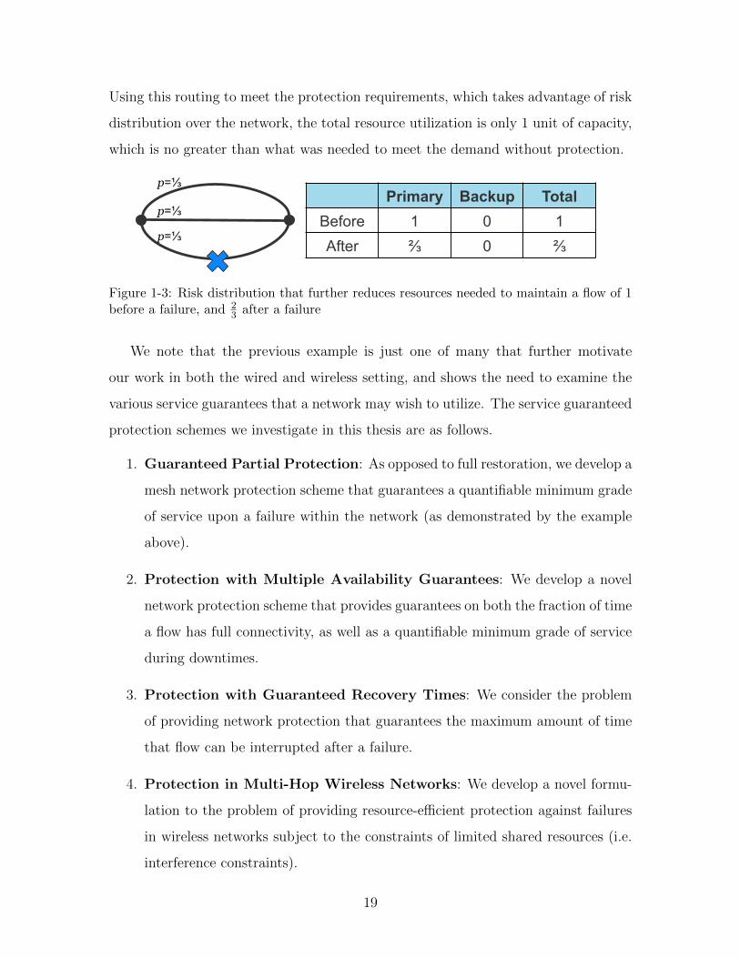
Using this routing to meet the protection requirements, which takes advantage of risk

distribution over the network, the total resource utilization is only 1 unit of capacity,

which is no greater than what was needed to meet the demand without protection.

p=⅓

p=⅓

p=⅓

Primary Backup Total Before 1 0 1 After ⅔ 0 ⅔

Figure 1-3: Risk distribution that further reduces resources needed to maintain a flow of 1before a failure, and 2

3 after a failure

We note that the previous example is just one of many that further motivate

our work in both the wired and wireless setting, and shows the need to examine the

various service guarantees that a network may wish to utilize. The service guaranteed

protection schemes we investigate in this thesis are as follows.

1. Guaranteed Partial Protection: As opposed to full restoration, we develop a

mesh network protection scheme that guarantees a quantifiable minimum grade

of service upon a failure within the network (as demonstrated by the example

above).

2. Protection with Multiple Availability Guarantees: We develop a novel

network protection scheme that provides guarantees on both the fraction of time

a flow has full connectivity, as well as a quantifiable minimum grade of service

during downtimes.

3. Protection with Guaranteed Recovery Times: We consider the problem

of providing network protection that guarantees the maximum amount of time

that flow can be interrupted after a failure.

4. Protection in Multi-Hop Wireless Networks: We develop a novel formu-

lation to the problem of providing resource-efficient protection against failures

in wireless networks subject to the constraints of limited shared resources (i.e.

interference constraints).

19

1.1 Background

Traditional network protection consists of two main approaches: restoration and pro-

tection [5]. Restoration and protection differ by when they allocate resources for

failure recovery. Restoration seeks to find unused resources in the network after a

network failure occurred in order to reroute the failed connections. Protection, on

the other hand, allocates resources for backup prior to a link failure. A notable ex-

ample of a restoration scheme is IP rerouting, where after a link failure occurs, the

network is updated with the new set of shortest paths between node pairs, and then

a new path is selected [10]. This is both slow (sometimes on the order of minutes)

[11], and does not necessarily guarantee that bandwidth will be available for the new

path [12, 13]. Restoration is not limited to the IP layer, and has been utilized in

other settings as well [14, 15]. Protection on the other hand allocates resources for

recovery prior to any link failure; this guarantees that backup resources are available

upon a failure. Additionally, since backup resources are already allocated for network

protection, no time is needed to “discover” unused capacity for recovery, which signif-

icantly reduces the time to recover after a failure. Pre-allocating resources comes at

the expense of additional complexity and resource utilization, but offers guarantees

that restoration cannot provide. In this thesis, we focus on network protection with

service guarantees, as opposed to network restoration, which cannot offer any such

guarantees.

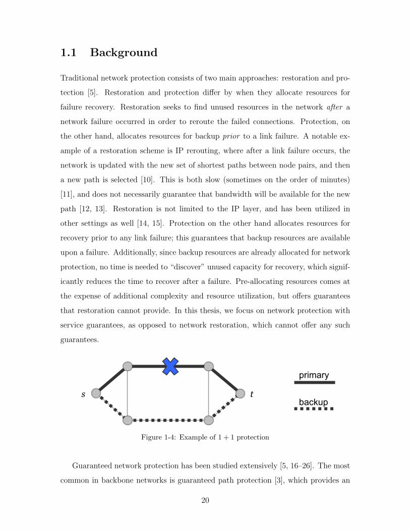
primary

backup s t

Figure 1-4: Example of 1 + 1 protection

Guaranteed network protection has been studied extensively [5, 16–26]. The most

common in backbone networks is guaranteed path protection [3], which provides an

20

edge-disjoint backup path for each primary path, resulting in 100% service recovery

after any link failure. This scheme is typically referred to as 1 + 1 protection [27],

and has one primary path to route traffic before a failure, and one backup path for

traffic after a failure. An example of 1 + 1 protection is shown in Figure 1-4.

Optimization theory is a tool that we extensively use to investigate network protec-

tion with service guarantees. Network related optimization problems are oftentimes

formulated as linear programs [28, 29]. A classic network flow problem is to find the

shortest path between a source node s, and destination node d. This basic formula-

tion to find the shortest path between s and d for some given graph G, with a set of

edges E and a set of vertices V , is shown below.

Objective: min∑{i,j}∈E

xij (1.1)

Subject to:∑{i,j}∈E

xij −∑{j,i}∈E

xji =

1 if i = s

−1 if i = d

0 otherwise

, ∀i ∈ V (1.2)

xij = {0, 1}, ∀{i, j} ∈ E (1.3)

The variables xij indicate whether or not an edge {i, j} in the network is used

(Constraint 1.3). The objective is to minimize the amount of flow across all of the

edges in order to route a unit of flow from s to d (Equation 1.1). The network flow

constraints are given by Constraint 1.2, which indicate that at any given node, the

flow into that node must be equal to flow out, except for the source and destination

node that will have 1 unit of flow in, and 1 unit of flow out, respectively. We note

that in this particular case, the linear program is in fact an integer linear program,

since the values of xij can only be 0 or 1.

Numerous shortest path algorithms exist that do not use a linear programming

formulation, such as Dijkstra or Bellman-Ford [29, 30], While these algorithms are

efficient, they typically do not allow any additional parameters or constraints to the

problem. Consider a modification to the shortest path problem that adds a service

21

guarantee: instead of simply finding the shortest path, we wish to find a shortest

path such that the total traversal time across all of the edges in that path do not

exceed some parameter T . It is not entirely clear how this can be done using one of

the aforementioned shortest path algorithms since they do not take into account any

such additional parameters. If each edge {i, j} has a traversal time of tij, then we can

simply modify the integer linear program above by adding the additional constraint.

∑{i,j}∈E

tijxij ≤ T (1.4)

Constraint 1.4 ensures that the sum of all of the edges used in a network will

not exceed the maximum path traversal time T . While integer linear programs are

typically inefficient to solve directly [31], such formulations allow us to develop optimal

solutions which include additional service guarantees, and allow us to begin analyzing

the problem and develop efficient algorithms for its solution. An algorithm for the

time-guaranteed shortest path (more commonly known as the constrained shortest

path problem) was developed using this exact approach in [32].

To further emphasize the utility of linear programming approaches to formulating

and solving a problem, we consider another important example: finding the shortest-

pair of disjoint paths, which as discussed above, is one of the primary schemes used to

protect networks. A naive approach would be to find a shortest path using one of the

many available algorithms, remove those edges, and then find another shortest path.

If a solution is returned, it will indeed be a pair of disjoint paths; unfortunately, this

approach may yield a non-optimal solution, or in some cases, no solution whatsoever

when one in fact does exist. Consider the network below in Figure 1-5.

s d

Figure 1-5: Example network for disjoint paths

22

If we used the approach described above (find the shortest path, remove those

edges, find the next shortest path), we see in Figures 1-6a and 1-6b that no second

path exists. But it is clear that two disjoint paths do exist, as seen in Figure 1-6c.

This example is a well known network commonly referred to as the “trap” topology

[33].

s d

(a) Shortest path

s d

(b) Network with shortest path removed

s d

(c) Network with two disjoint paths

Figure 1-6: Finding disjoint paths in the trap topolgoy

If in the above linear program, Constraint 1.2 is modified to Constraint 1.5 (seen

below), then 2 units of flow must traverse from the source to destination. Since any

edge can only have a flow of 0 or 1 (Constraint 1.3), no two paths can use the same

edge, and two disjoint paths are guaranteed when solving the integer linear program.

∑{i,j}∈E

xij −∑{j,i}∈E

xji =

2 if i = s

−2 if i = d

0 otherwise

, ∀i ∈ V (1.5)

Examining the structure of the above linear program allows us to further under-

stand the problem, which then allows for efficient algorithmic solutions, as was done

23

for the shortest pair of disjoint paths problem in [21, 34]. Linear programs, and in

particular integer linear programs, are often inefficient to solve. Powerful tools do

exist for solving linear and integer linear program [35], though their running times

are not guaranteed. But formulating our problems in such a fashion allows us to con-

sider additional service guarantees, and then analyze the effects that these additional

guarantees/constraints have on our problem. This approach often times allows us to

find efficient algorithmic solutions to the problem that otherwise may have seemed

intractable.

We next consider wireless networks and the additional challenges they impose.

As opposed to wired networks, two nodes in a wireless network that are within close

proximity of one another cannot transmit simultaneously, or else those transmissions

will interfere. So, in addition to finding a route, a schedule of link transmissions needs

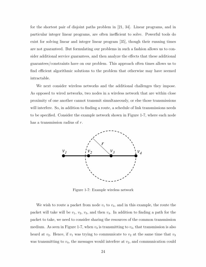
to be specified. Consider the example network shown in Figure 1-7, where each node

has a transmission radius of r.

v3 v4 v1 v2 r

Figure 1-7: Example wireless network

We wish to route a packet from node v1 to v4, and in this example, the route the

packet will take will be v1, v2, v3, and then v4. In addition to finding a path for the

packet to take, we need to consider sharing the resources of the common transmission

medium. As seen in Figure 1-7, when v3 is transmitting to v4, that transmission is also

heard at v2. Hence, if v1 was trying to communicate to v2 at the same time that v3

was transmitting to v4, the messages would interfere at v2, and communication could

24

not occur. Similarly, it can be seen that v2 cannot be transmitting to v3 while v3 is

transmitting to v4. In order to have successful communication without interference,

links need to be scheduled to transmit during non-overlapping time slots, such that

no two links within transmission range will communicate simultaneously. For our

example, if we divide time into three time slots, link {v1, v2} will be active during the

first time slot, {v2, v3} will be active during the second time slot, and {v3, v4} will be

active during the third time slot. With such a transmission schedule, interference-free

communication is possible.

The key hurdle to finding an interference-free schedule is that the complexity that

is added is substantial. Not only do we wish to find a route and a schedule, but

we typically want to find a minimum-length schedule. The smaller fraction of time

that a link can transmit, the lower its overall throughput will be. Hence, finding a

minimum-length schedule is akin to finding a schedule that maximizes throughput.

Because of these considerations, wireless routing and scheduling belongs to the class

of non-polynomial time solvable problems [36] known as NP-hard [37]. It is within

these additional set of interference constraints that we try to find resource-efficient

protection for wireless networks.

1.2 Contributions

We now give a greater overview of the problems considered and the contributions of

the thesis.

1.2.1 Guaranteed Partial Protection

In Chapter 2, we develop a novel mesh network protection scheme that guarantees a

quantifiable minimum grade of service upon a failure within the network. Typically,

networks fully guarantee service after a single-link failure, which is often an over-

provisioning of resources to maintain essential traffic for the infrequent event of a

failure. Our scheme guarantees that a fraction q of each demand is maintained after

any single-link failure, at a small fraction of the cost of full protection.

25

An example of the partial protection service guarantee was presented earlier in

Figures 1-1, 1-2, and 1-3, which demonstrates the significant savings that can be

achieved by taking advantage of the redundancy and self-protection that is inherently

available in mesh networks.

A linear program is developed to find the minimum-cost capacity allocation to

meet both the demand and protection requirements. For a partial protection re-

quirement of q ≤ 12, an exact algorithmic solution for the minimum-cost routing and

capacity allocation is developed using multiple shortest paths. For q > 12, an algo-

rithm is developed based on disjoint path routing that performs, on average, within

1.4% of optimal, and runs four orders of magnitude faster than the minimum-cost

solution achieved via the linear program. Furthermore, we demonstrate that our

algorithm is guaranteed to give a solution whose cost is at most twice that of the

optimal solution. The partial protection strategies developed in this chapter achieve

reductions of up to 83% in spare capacity as compared to traditional full protection

schemes.

The contribution we make in this chapter is developing a “theory” for partial pro-

tection that includes optimal algorithms for capacity allocation, as well as explicit

expressions for the amount of required additional backup capacity. In Section 2.2, the

partial protection model is described. In Section 2.3, the partial protection problem

is formulated as a linear program with the objective of finding the minimum-cost allo-

cation of primary and backup capacity. In Section 2.4, solutions for partial protection

without the use of backup capacity sharing are developed, including a simple path

based routing for an optimal solution when q ≤ 12, and when q > 1

2, properties of an

optimal solution for a network of disjoint paths are determined and used to develop

a time-efficient algorithm. In Section 2.5, backup capacity sharing is considered, and

an algorithm is developed for the case of dynamic (one-at-a-time) arrivals.

1.2.2 Protection with Multiple Availability Guarantees

In Chapter 3, we develop a novel network protection scheme that provides guarantees

on both the fraction of time a flow has full connectivity, as well as a quantifiable

26

minimum grade of service during downtimes. In particular, a flow can be below the

full demand for at most a maximum fraction of time; then, it must still support

at least a fraction q of the full demand. This is in contrast to current protection

schemes that offer either availability-guarantees with no bandwidth guarantees during

the downtime, or full protection schemes that offer 100% availability after a single

link failure.

(a) 1 + q partial protection (b) 1 + 1 full protection

Figure 1-8: Comparison of Multiple Availability Guaranteed Protection (MAGP) vs. tra-ditional protection schemes

To further motivate the problem, consider the example in Figure 1-8, with link

failure probabilities and flow allocations as labeled (p and f respctively). A unit

demand needs to be routed from s to t, and this connnection can drop to its partial

protection requirement q after a failure with at most a probability of 14. In Chapter

2, we introduced a simple partial protection scheme called 1 + q protection that

routes the primary demand on one path and the partial protection requirement onto

another edge-disjoint path. After any failure along the primary path, the partial

protection requirement is met. This routing is shown in Figure 1-8a, with the solid

line carrying the primary flow of 1 and the dotted line carrying the protection flow

of q. However, in this routing, the maximum failure probability is exceeded: after a

failure, the flow drops below the unit demand between s and t with a probability of

12

(because the failure of either of the primary links would drop the demand below

its full capacity). A naive alternative would be to simply allocate another path for

protection, which would be identical to the 1 + 1 full protection scheme (shown in

Figure 1-8b), and utilize a total of 4 units of capacity. After any failure, the full

flow of 1 unit is maintained; thus, the user will face no downtime, which meets and

exceeds the maximum probability of failure requirement of 14.

27

If we allow different levels of protection on different segments of the primary path,

then a more resource efficient allocation is possible. Consider keeping the primary

flow on the same bottom two edges as before, but instead of allocating an end-to-end

backup path along the top two edges, 1 unit of flow is allocated to protect against

the failure of {s, v} and q units of flow to protect against the failure of {v, t} (shown

in Figure 1-9). If after some disruption either of the {s, v} edges fail, 1 unit of flow

will still remain from s to t. By fully protecting the primary {s, v} edge, there is zero

probability that its failure will cause the flow to drop below the full demand. The

probability that the flow will drop below 1 after some failure is 14, which meets the

requirement that flow can drop to q with at most a probability of 14

after a failure.

This routing only needs 3 + q units of capacity, as opposed to the 4 units of capacity

that full protection requires.

Figure 1-9: Routing with a probability of 14 for the flow to drop to q after a failure

The novel contributions of Chapter 3 include the development of a framework

for Multiple Availability Guaranteed Protection (MAGP), and the development of

associated algorithms for both the cases when protection resources can and cannot

be shared. We show that the multiple availability guaranteed problem is NP-Hard,

and develop an optimal solution in the form of an MILP. If a connection is allowed

to drop to 50% of its bandwidth for just 1 out of every 20 failures, then a 24%

reduction in spare capacity can be achieved over traditional full protection schemes.

Allowing for more frequent drops to partial flow, additional savings can be achieved.

Algorithms are developed that provide multiple availability guarantees for both the

sharing and non-sharing case. For the case of q = 0, corresponding to the standard

availability constraint, an optimal pseudo-polynomial time algorithm is presented.

Chapter 3 is organized as follows. In Section 3.2, the model for Multiple Avail-

ability Guaranteed Protection (MAGP) is described. In Section 3.3, MAGP is shown

28

to be NP-Hard, and the minimum-cost solution to MAGP is formulated as an MILP.

In Section 3.4, optimal solutions and algorithms for MAGP are developed when pro-

tection resources cannot be shared, and in Section 3.5, an algorithm is developed for

when protection resources can be shared.

1.2.3 Protection with Guaranteed Recovery Times using Re-

covery Domains

In Chapter 4, we consider the problem of providing resource-efficient network protec-

tion that guarantees the maximum amount of time that flow can be interrupted after

a failure. This is in contrast to schemes that offer no recovery time guarantees, such

as IP rerouting, or the prevalent local recovery scheme of Fast ReRoute (FRR), which

often over-provisions resources to meet recovery time constraints. To meet these re-

covery time guarantees, we provide a novel and flexible solution by partitioning the

network into failure-independent “recovery domains”, where within each domain, the

maximum amount of time to recover from a failure is guaranteed.

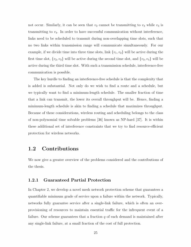
The most common protection scheme that tries to ensure fast recovery times is a

local recovery scheme known as Fast ReRoute (FRR) [38]. In FRR, after a failure,

traffic is routed away from the node directly upstream from a fault, and reconnects

the rerouted traffic with the original path at some downstream node. An example is

shown in Figure 1-10.

33

links and to quickly recover from a failure [35]. With QoS, traffic can receive different priorities and

different recovery times. The goal recovery time for recoverable traffic in MPLS is 50 ms [36], which

will allow data loss to be minimal during a failure. Because of its flexibility and traffic engineering

capabilities, MPLS has become the leading packet transport network technology in backbone networks

[37].

(a) Local Repair (b) Facility Backup

Figure 17: MPLS Fast Reroute Schemes

To handle these fast recovery times, the MPLS Fast Reroute (FRR) framework was developed [38].

Two different protection mechanisms are offered: local repair and facility backup. In local repair (Figure

17a), traffic is routed away from the node directly preceding a fault, known as the point of local repair

(PLR), and reconnects with the original path at the merge point (MP). In facility backup (Figure 17b),

a single recovery path is used to backup many primary paths that have the same QoS requirements.

For a newer specification, MPLS-TP, protection needs to be provided to recovery domains [39]. If a

path fails, then an alternate path will be taken from one end of the recovery domain to the other, as

shown in Figure 18.

Figure 18: MPLS-TP Recovery Domains

Depending on the QoS parameters of the demand, different protection paths may be used to route

Figure 1-10: Fast ReRoute (FRR)

In Fast ReRoute, since each possible failure has its own dedicated protection

path, resources are often over-provisioned beyond what is needed to meet recovery

time guarantees. Consider the network shown Fig. 1-11, where the propagation delay

for each link is 10 ms, and switching delays are assumed to be negligible. A flow

29

v1 v2 v3 v4 v5

Figure 1-11: Time guaranteed recovery examples

needs to be routed from v1 to v5 such that the maximum time that the flow can be

disrupted after a failure is 50 ms, which is the typical recovery time for backbone

networks [11]. A primary path is already allocated on the solid lines from v1 to v5.

A solution to FRR local recovery is to use all of the links above the primary path:

after a link failure in the primary path, a fault notification is sent to the immediate

upstream node of that failed link, and the flow is then switched to an alternate path

from that node back towards the destination. This protection scheme requires 7 edges

to be used for backup.

Recovery Domain 1

Recovery Domain 2

Recovery Domain 3

Figure 1-12: End-to-end routing using recovery domains

More recently, the new IETF standard for a backbone network protection frame-

work calls for the creation of “recovery domains” [39]. Recovery domains are defined

to be non-overlapping path segments, such that after a failure within a segment, flow

is restored using a back-up path between the end-points of that segment. Moreover,

recovery domains connect to one another via their respective “reference” end-points,

30

forming an end-to-end protected flow. An example is shown in Fig. 1-12: after the

failure of an edge in the primary path located within Recovery Domain 2, the re-

covery domain’s upstream end-point redirects flow onto the backup path, which then

reconnects at that recovery domain’s downstream end-point, bypassing the failure.

Now consider an alternative protection routing for the network in Figure 1-11

using the recovery domain model. Two recovery domains are created by using the

links below the primary path as the backup paths: one recovery domain between

nodes v1 and v3, and one between v3 and v5. If link {v2, v3} fails, it would take up

to 20 ms for the fault notification to propagate to v1, and then 20 ms for the data

that was switched to the protection route to reconnect with the primary path at node

v3. The other recovery domain will have a similar recovery time after a failure. In

this example, only 4 additional links are needed to meet protection guarantees when

using recovery domains, as opposed to the 7 needed for FRR.

To the best of our knowledge, this work is the first to investigate Guaranteed

Recovery Times using Recovery Domains (GRT-RD). The outline of Chapter 4 is

as follows. We first present a model of the problem in Section 4.2. We then show

in Section 4.3 that the recovery domain problem is NP-Hard, and formulate the

optimal solution using an MILP. This provides protection with guaranteed recovery

times using up to 45% less protection resources than local recovery. In Section 4.4, we

decompose the end-to-end recovery domain problem into more tractable subproblems,

which allows us to more easily construct a solution for the end-to-end problem. This

allows for the development of flexible and efficient solutions, including an optimal

algorithm using Lagrangian relaxation, which simulations show to converge rapidly

to an optimal solution. In Section 4.5, an algorithm is developed for the case when

backup sharing is allowed. For dynamic arrivals, this algorithm performs better than

the solution that tries to greedily optimize for each incoming demand.

1.2.4 Providing Protection in Multi-Hop Wireless Networks

In Chapter 5, we consider the problem of providing protection against failures in

wireless networks subject to interference constraints. Typically, protection in wired

31

networks is provided through the provisioning of backup paths. This approach has

not been previously considered in the wireless setting due to the prohibitive cost

of reserving limited resources for backup capacity. However, we show that in the

presence of transmission interference, protection can often be provided with no loss

in throughput. This is due to the fact that after a failure, links that previously

interfered with the failed link can be activated, thus leading to a “recapturing” of

some of the lost capacity.

The addition of interference constraints makes the protection problem in a wireless

setting fundamentally different from the ones found in a wired context. After a failure

in a wireless network, links that could not have been used due to interference with

the failed link become available, and can be used to recover from the failure.

s d

a

b

c

1

2 1

2

(a) Before a failure

s d

a

b

c

1

2 1

2

(b) After {s, b} fails

Figure 1-13: Time slot assignment for protection in a wireless network

Consider allocating a protected flow between nodes s and d for the network shown

in Figure 1-13. We assume an interference model where any two links that have a

node in common cannot be active at the same time (often referred to as the 1-hop

interference model [40]). Additionally, we assume unit capacity links. Before any

failure, the maximum flow from s to d is 1, which can be achieved by scheduling

the network into two distinct time slots such that transmissions can occur without

interfering with one another, with the time slot assignment shown in Figure 1-13a.

At any given point in time, only one outgoing link from s can be active, and similarly,

only one incoming link to d can be active. Wireless links {s, c}, and {c, d} cannot be

used prior to the failure of {s, b}, but become available after {s, b} fails. After the

32

failure of {s, b}, flow can be routed from s to c during time slot 2, and from c to d

during slot 1, as shown in Figure 1-13b. Similar schedules can be found for failures

of the other links. The maximum flow from s to d is 1 for both before and after a

failure; i.e., there is no reduction in maximum throughput when allocating resources

for a protection route on {s, c} and {c, d}: protection can be assigned for “free”. This

is in contrast to a wired network where the maximum throughput without protection

from s to d is 3, and the maximum throughput when assigning a protection route on

{s, c} and {c, d} is 2, which amounts to a 13

loss in throughput due to protection.

The novel contribution of Chapter 5 is in introducing the Wireless Guaranteed

Protection (WGP) problem in multi-hop networks with interference constraints. We

show that the general problem of optimal routing and scheduling with protection is

NP-hard, and provide both an ILP formulation for the optimal solution, as well as

algorithms that perform close to optimal. More importantly, we show that providing

protection in a wireless network uses as much as 72% fewer protection resources as

compared to similar protection schemes designed for wired networks, and that in

many cases, no additional resources for protection are needed.

Chapter 5 is outlined as follows. In Section 5.2, the model for WGP is presented.

In Section 5.3, properties of an optimal solution are examined for a single demand

with 1-hop interference constraints, which are then used to motivate the development

of a time efficient algorithm that guarantees a solution with 1.5 of optimal. In Section

5.4, an optimal solution is developed via a mixed integer linear program for general

interference constraints. In Section 5.5, time-efficient algorithms are developed that

perform within 4.5% of the optimal solution.

33

Chapter 2

Guaranteed Partial Protection

2.1 Introduction

Mesh networks with ever-increasing data rates are being deployed to meet the in-

creasing demands of the telecommunication industry. As data rates continue to rise,

the failure of a network line element or worse, a fiber cut, can result in severe service

disruptions and large data loss, potentially causing millions of dollars in lost revenue

[2]. Currently, there exist few options for protection that offer less than complete

restoration after a failure. Due to the cost of providing full protection, many service

providers offer no protection whatsoever. Additionally, since fiber cuts are relatively

uncommon and are on average repaired quickly [4, 9], service providers may wish

to only support essential traffic after a network failure. By defining varying and

quantifiable grades of protection, service providers can protect vital services without

incurring the cost of providing full protection, making protection more affordable and

better suited to user/application requirements. The protection scheme developed in

this chapter provides “partial protection” guarantees, at a fraction of the cost of full

protection, with each session having its own differentiated protection guarantee.

Guaranteed network protection has been studied extensively [5, 16–20]. The most

common in backbone networks today is guaranteed path protection [3], which pro-

vides an edge-disjoint backup path for each primary path, resulting in 100% service

restoration after any link failure. Best effort protection is still loosely defined, but

35

generally offers no guarantees on the amount of protection provided. In best effort

protection, a service will be protected, if possible, with any unused capacity after fully

protecting all guaranteed services [4, 41]. Best effort protection can also be referred to

as partial capacity restoration, since a service will be restored within existing unused

capacity, typically resulting in less than 100% restoration.

Many users may be willing to tolerate short periods of reduced capacity to protect

only essential services if data rate guarantees can be made at a reduced cost. In this

chapter, we consider an alternate form of guaranteed protection, where a fraction of

a demand is guaranteed in the event of a link failure. If provided at a reduced cost,

many users may opt for partial protection guarantees during network outages.

A quantitative framework for deterministic partial protection in optical networks

was first developed in [42]. In this work, a minimum fraction q of the demand is

guaranteed to remain available between the source and destination after any single

link failure, where q is between 0 and 1. When q is equal to 1, the service is fully

protected, and when q is 0, the service is unprotected. More recently, [43] examines the

savings that can be achieved by guaranteeing part of the demand in the event of a link

failure, as opposed to full protection. It shows that the amount of protection that can

be guaranteed depends on the topology of the network. In [44], the partial protection

problem on groomed optical WDM networks is studied, under the assumption that

flows must traverse a single path.

In this chapter, we further expand upon the framework developed in [42]. We de-

velop a “theory” for partial protection that includes optimal algorithms for capacity

allocation, and explicit expressions for the amount of required additional backup ca-

pacity. Routing strategies that allocate working and backup capacity to meet partial

protection requirements are derived. Similar to [43], flow bifurcation over multi-

ple paths is allowed. Bifurcation reduces the amount of additional backup capacity

needed to support the protection requirements. In fact, we show that depending on

the value of q, it may be possible to provide protection without any additional backup

capacity at all.

A linear program is developed to find the optimal minimum-cost capacity alloca-

36

tion needed to guarantee partial protection in the event of a link failure. Without

backup capacity sharing, a routing and capacity assignment strategy based on short-

est paths is shown to be optimal for q ≤ 12. For q > 1

2, an efficient algorithm based

on disjoint path routing is shown to have a cost that is at most twice the optimal

minimum-cost solution, and in practice only slightly above optimal. For the case with

backup capacity sharing, we show that depending on the value of q, it may be pos-

sible to provide protection at minimal allocation cost, i.e. the shortest path routing.

We consider two cases: preemptive and non-preemptive partial protection. For the

preemptive case, primary resources available prior to a link failure may be preempted

to provide backup for other demands, as long as all protection requirements are met

after the failure. For the non-preemptive case, only demands that are directly affected

by the link failure drop to the rates guaranteed under partial protection.

In Section 2.2, the partial protection model is described. In Section 2.3, the partial

protection problem is formulated as a linear program with the objective of finding the

minimum-cost allocation of primary and backup capacity. In Section 2.5, solutions for

partial protection without the use of backup capacity sharing are developed, including

a simple path based routing for an optimal solution when q ≤ 12, and when q > 1

2,

properties of an optimal solution for a network of disjoint paths are determined and

used to develop a time-efficient algorithm. In Section 2.5, backup capacity sharing

is considered, and an algorithm is developed for the case of dynamic (one-at-a-time)

arrivals.

2.2 Partial Protection Model

The objective of partial protection is to find an allocation that ensures that enough

capacity exists to support the full demand before a link failure and a fraction q of

that demand afterward. We assume that the graph G, with a set of vertices V and

edges E, is at least two-connected. Each link has a fixed cost of use: cij for each

edge {i, j} ∈ E. We consider only single link failures. Both primary traffic and

protection flows (defined as the flow after a failure) can be bifurcated to traverse

37

multiple paths between the source and destination. Without loss of generality, we

assume unit demands, unless noted otherwise.

To begin with, assume that link costs are all 1; in the next section we will consider

non-uniform link costs. With uniform link costs, the objective is to minimize the total

capacity needed to support the flow and the partial protection requirements.

(a) 1 + 1 protection (b) 1 + q protection, q = 23

Figure 2-1: Standard protection schemes

One routing strategy for providing backup capacity is to use a single primary

path and a single backup path similar to the 1+1 guaranteed path protection scheme.

Consider the network shown in Figure 2-1. With 1+1 protection, one unit of capacity

is routed on a primary path and one unit of capacity on a backup (Figure 2-1a). Upon

a link failure, 100% of the service can be restored via the backup path. Now, consider

a partial protection requirement to provide a fraction q = 23

of backup capacity in the

event of a link failure. A simple protection scheme similar to 1 + 1 protection would

be to route one unit along the primary path and 23

along a disjoint protection path,

as shown in Figure 2-1b. We will refer to this protection scheme as 1 + q protection.

If the primary path fails, sufficient backup capacity remains to provide service for 23

of the demand.

(a) q = 1 (b) q = 23

Figure 2-2: Protection using risk distribution

38

For both partial and full protection requirements, in many cases capacity savings

can be achieved if the risk is distributed by spreading the primary allocation across

multiple paths. For example, by spreading the primary allocation across the three

available paths, as shown in Figure 2-2a, any single link failure results in a loss of at

most 13

of the demand. To fully protect this demand against any single link failure

(i.e. q = 1), additional spare capacity allocation1 of s = 16

needs to be added to each

link. With this strategy, a total of 1.5 units of capacity are required, as opposed to

the total of 2 units needed by 1 + 1 protection. If instead the protection requirement

was q = 23, no spare allocation is needed since after any failure 2

3units are guaranteed

to remain. By spreading the primary and backup allocation across the multiple paths

between the source and destination, the risk is effectively distributed and the fraction

of primary allocation lost by a link failure is reduced.

2.3 Minimum-Cost Partial Protection

In this section, a linear program is developed to achieve an optimal minimum-cost

solution to the partial protection problem. The objective of the linear program is

to find a minimum-cost routing strategy to meet demand d and partial protection

requirement q for a set of demands. In particular, a demand’s full flow requirement

must be routed before any failure, and in the event of any link failure, a fraction q

of that flow must remain. Backup capacity sharing is utilized to further reduce the

capacity allocation (and cost) needed to meet demand and protection requirements.

If two demands’ primary paths are edge disjoint, then under a single link failure

model, only one demand can fail at a time. Hence, backup capacity can be shared

between the two since at most one demand will need to use it at any given point in

time. The linear program to solve for the optimal routing strategy, denoted LPPP ,

is defined below. We start by considering the case where only primary demands that

are directly affected by a failure are switched to their respective protection flows (no

1We define spare capacity allocation to be the capacity that must be allocated in addition to thenecessary capacity used to support the primary demand before a link failure.

39

preemption). Afterwards, the linear program is modified to allow for primary capacity

to be preempted after a failure to route protection flows, so long as all demands have

their protection requirements met.

2.3.1 Linear Program to Meet Partial Protection: LPPP

The following values are given:

• G = (V,E,C) is the graph with its set of vertices, edges, and costs

• dst is the total demand between nodes s and t

• qst is the fraction of the demand between s and t that must be supported on

the event of a link failure

• cij is the cost of link {i, j}

The LP solves for the following variables:

• xstij is primary flow on link {i, j} for demand (s, t), xstij ≥ 0

• f stij,kl is the protection flow on link {i, j} after the failure of link {k, l} for demand

(s, t), f stij,kl ≥ 0

• ystij,kl is the spare capacity for demand (s, t) on link {i, j} for failure of link {k, l},

ystij,kl ≥ 0

• wij is total primary flow on link {i, j}, wij ≥ 0

• sij is total spare allocation on link {i, j}, sij ≥ 0

The objective of LPPP is to minimize the cost of allocation over all links:

min∑{i,j}∈E

cij(wij + sij) (2.1)

Subject to the following constraints:

40

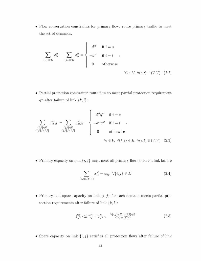
• Flow conservation constraints for primary flow: route primary traffic to meet

the set of demands.

∑{i,j}∈E

xstij −∑{j,i}∈E

xstji =

dst if i = s

−dst if i = t

0 otherwise

,

∀i ∈ V, ∀(s, t) ∈ (V, V ) (2.2)

• Partial protection constraint: route flow to meet partial protection requirement

qst after failure of link {k, l}:

∑{i,j}∈E{i,j}6={k,l}

f stij,kl −∑{j,i}∈E{j,i}6={k,l}

f stji,kl =

dstqst if i = s

−dstqst if i = t

0 otherwise

,

∀i ∈ V, ∀{k, l} ∈ E, ∀(s, t) ∈ (V, V ) (2.3)

• Primary capacity on link {i, j} must meet all primary flows before a link failure

∑(s,t)∈(V,V )

xstij = wij, ∀{i, j} ∈ E (2.4)

• Primary and spare capacity on link {i, j} for each demand meets partial pro-

tection requirements after failure of link {k, l}:

f stij,kl ≤ xstij + ystij,kl,∀{i,j}∈E, ∀{k,l}∈E∀(s,t)∈(V,V ) (2.5)

• Spare capacity on link {i, j} satisfies all protection flows after failure of link

41

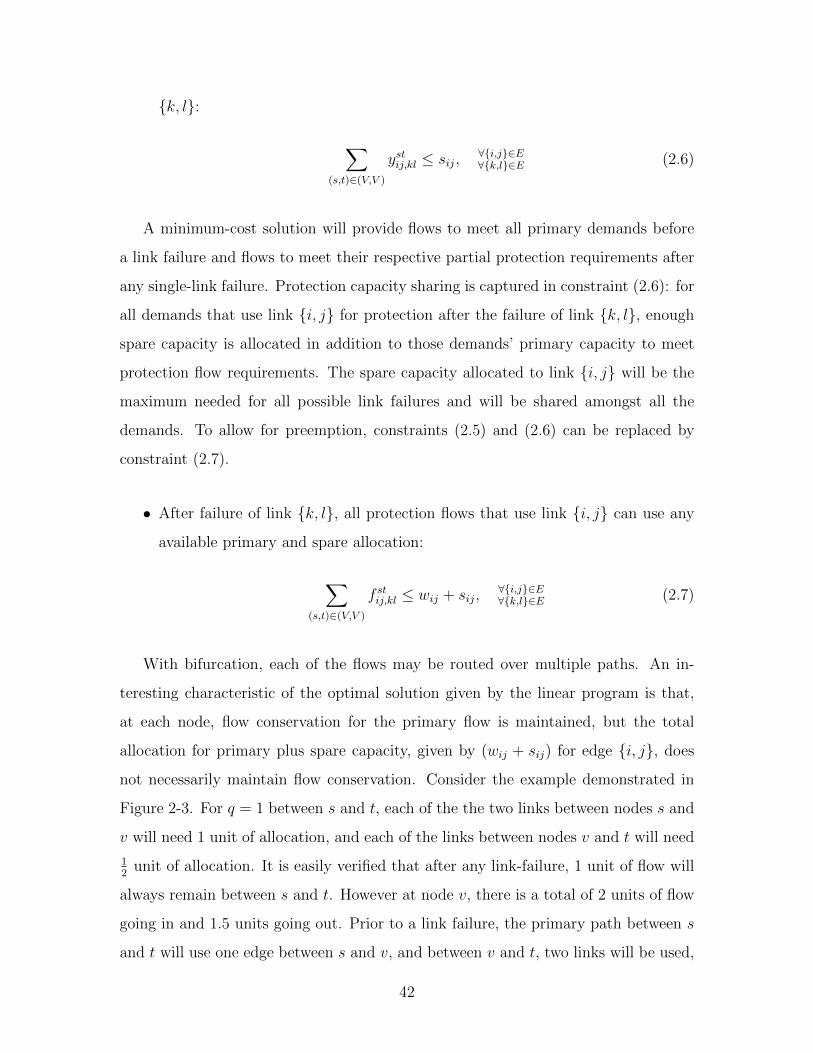
{k, l}:

∑(s,t)∈(V,V )

ystij,kl ≤ sij,∀{i,j}∈E∀{k,l}∈E (2.6)

A minimum-cost solution will provide flows to meet all primary demands before

a link failure and flows to meet their respective partial protection requirements after

any single-link failure. Protection capacity sharing is captured in constraint (2.6): for

all demands that use link {i, j} for protection after the failure of link {k, l}, enough

spare capacity is allocated in addition to those demands’ primary capacity to meet

protection flow requirements. The spare capacity allocated to link {i, j} will be the

maximum needed for all possible link failures and will be shared amongst all the

demands. To allow for preemption, constraints (2.5) and (2.6) can be replaced by

constraint (2.7).

• After failure of link {k, l}, all protection flows that use link {i, j} can use any

available primary and spare allocation:

∑(s,t)∈(V,V )

f stij,kl ≤ wij + sij,∀{i,j}∈E∀{k,l}∈E (2.7)

With bifurcation, each of the flows may be routed over multiple paths. An in-

teresting characteristic of the optimal solution given by the linear program is that,

at each node, flow conservation for the primary flow is maintained, but the total

allocation for primary plus spare capacity, given by (wij + sij) for edge {i, j}, does

not necessarily maintain flow conservation. Consider the example demonstrated in

Figure 2-3. For q = 1 between s and t, each of the the two links between nodes s and

v will need 1 unit of allocation, and each of the links between nodes v and t will need

12

unit of allocation. It is easily verified that after any link-failure, 1 unit of flow will

always remain between s and t. However at node v, there is a total of 2 units of flow

going in and 1.5 units going out. Prior to a link failure, the primary path between s

and t will use one edge between s and v, and between v and t, two links will be used,

42

each with a capacity allocation of 12. After a link failure, similar allocations will be

used to maintain full flow. Hence the total flow to support the demand before and

after the link failure is conserved, however the capacity used to achieve this flow is

not conserved at v.

Figure 2-3: Example of flow not being conserved at node v

2.3.2 Comparison to Standard Protection Schemes

To compare the optimal solution to alternative protection schemes, two simulations

are run: one where backup capacity sharing is not allowed, and one where it is.

For the case without backup capacity sharing, 1000 random graph topologies are

generated, each containing 50 nodes with an average node degree of 3.1, and having

random link costs. Two nodes are randomly chosen from each graph to be the source

and destination. The minimum-cost partial protection routing, as found by LPPP ,

is compared to the standard scheme of 1 + 1 protection, as well as 1 + q protection.

By not allowing flow to bifurcate, i.e. xstij ∈ {0, 1}, ∀{i, j} ∈ E, the resulting scheme

would be 1 + q protection (and hence is now a mixed integer linear program). The

linear programs are solved by using the CPLEX solver. Suurballe’s algorithm [34] for

the shortest pair of disjoint paths were used to solve for 1 + 1 protection.

The average cost to route the demand and protection capacity using the different

routing strategies are plotted in Figure 2-4 as a function of q. The top line, showing

capacity requirements under 1 + 1 protection, remains constant for all values of q.

The next two lines from the top are 1 + q and LPPP , respectively. As expected, both

meet demand and protection requirements using fewer resources than 1 + 1, however,

the minimum-cost solution produced by the partial protection linear program that

43

10

15

20

25

30

35

0 0.1 0.2 0.3 0.4 0.5 0.6 0.7 0.8 0.9 1

Cos

t

q

1+1 1+q LP q=0

PP

Shortest Path

Figure 2-4: Without protection sharing: capacity cost vs. q

allows flow to bifurcate uses significantly less capacity. A lower bound on the capacity

requirement is the shortest path routing, which provides no protection (shown in the

bottom line of the figure). The cost of providing partial protection q is the difference

between the cost of the respective protection strategies and the shortest path routing.

Our partial protection scheme achieves reductions in excess resources of 82% at q = 12

to 12% at q = 1 over 1 + 1 protection, and 65% at q = 12

to 12% at q = 1 over 1 + q

protection.

For the case when backup capacity sharing is allowed, we compare both preemptive

and non-preemptive partial protection with the 1 + 1 and 1 + q protection schemes,

which now allow for backup capacity sharing. The various partial protection schemes

are compared via simulation using the NSFNET topology (Fig. 2-6) with 100 random

unit demands. The protection requirement, q, for each demand has a truncated

normal distribution with standard deviation σ = 12. The mean of q is varied between

0 and 1 for each iteration.

The average costs to route the demand and protection capacity using the different

routing strategies are plotted in Fig. 2-5 as a function of the expected value of q.

Once again, the shortest path routing without protection considerations is used as a

44

200

220

240

260

280

300

320

340

360

0 0.25 0.5 0.75 1

Cos

t

q

1+1 1+q Non-Preempt Preempt Shortest Path

Figure 2-5: With protection sharing: capacity cost vs. q

lower bound for the allocation cost. In this simulation, preemptive partial protection

is able to meet requirements using only the capacity needed for the shortest path

routing for q ≤ 12, and only an additional increase in total capacity of 2% for q ≤ 3

4.

When considering savings in excess resources, preemptive partial protection achieves

reductions of 83% at q = 1 over both 1 + 1 protection and 1 + q protection. Non-

preemptive shared partial protection, at q = 12, achieves reductions in excess resources

of 59% over 1 + 1 shared protection and 19% over 1 + q shared protection.

2

1

3

45

6

7

8

9

10

11

12

13

14

Figure 2-6: 14 Node NSFNET backbone network

45

2.4 Solutions without Backup Capacity Sharing

In this section, we provide insights on the structure of the solution to the minimum-

cost partial protection problem when backup capacity sharing cannot be utilized.

In Section 2.4.1, we are able to derive an exact algorithmic solution to the partial

protection problem for q ≤ 12, which runs in polynomial time using a simple series of

shortest paths. When q > 12, we analyze solutions for a simpler two-node networks in

Section 2.4.2. Using these insights for a two-node network for q > 12, combined with

the exact solution for q ≤ 12, a time-efficient algorithm is developed in Section 2.4.3

for general mesh networks. In Section 2.5, the case when backup capacity sharing is

allowed is considered.

2.4.1 Solution for q ≤ 12

As mentioned in Section 2.2, the total primary and spare allocation coming in and

out of any given node for an optimal solution does not necessarily maintain flow

conservation. Without this property, most network flow algorithms do not apply [29]

and analysis of the linear program becomes difficult. We show that all minimum-cost

solutions for q ≤ 12

will never need spare allocation, hence allowing us to formulate

the partial protection problem using standard network flow conservation constraints.

This then allows us to derive a simple path-based algorithmic solution. All proofs for

this section are provided in Chapter Appendix Section 2.7.1.

We begin by demonstrating that spare capacity is never needed for an optimal

solution if the primary capacity on an edge is less than or equal to (1 − q). Hence,

any time a link fails, at least q remains in the network.

Lemma 2.1. No spare capacity is needed to satisfy the flow and protection require-

ments if and only if the primary capacity on each link is less than or equal to (1− q).

In Section 2.4.2, we show routings with zero spare allocation are not necessarily

lowest cost for all values of q. However, Lemma 2.2 shows that when q ≤ 12, the

minimum-cost solution will never use spare allocation.

46

Lemma 2.2. Given a demand between nodes s and t with a protection requirement

of q ≤ 12, all minimum-cost solutions have no spare capacity on any edge: sij =

0, ∀{i, j} ∈ E.

Combining Lemmas 2.1 and 2.2, it can be seen that a minimum-cost solution exists

that does not use any spare allocation for q ≤ 12, and that xij ≤ (1− q), ∀{i, j} ∈ E.

Since the problem can now be formulated for q ≤ 12

using no spare allocation, flow

conservation at each node is preserved. The linear program can now be written

using a standard flow formulation without the use of spare allocation. The modified

linear program, referred to as LPq≤.5, routes the flows on the paths in a manner that

minimizes total cost and ensures that no edge carries more than (1− q) of flow.

LPq≤.5 : min∑{i,j}∈E

cijxij (2.8)

∑{i,j}∈E

xij −∑{j,i}∈E

xji =

1 if i = s

−1 if i = t

0 otherwise

, ∀i ∈ V (2.9)

xij ≤ (1− q), ∀{i, j} ∈ E (2.10)

The above linear program achieves a minimum-cost routing in a network by using

only primary allocation to meet the demand. LPq≤.5 is a network flow problem

with directed and capacitated edges, which is recognized as a minimum-cost flow

problem [29], for which algorithmic methods exist for finding an optimal solution. In

Theorem 2.1, we show that an optimal solution for q ≤ 12

uses at most three paths

with allocation q on each of the shortest pair of disjoint paths and allocation (1− 2q)

on the shortest path.

Consider a directed graph G = (V,E) with a source s and destination t. Let p0

47

be the cost of the shortest path, p1 and p2 be the costs of the two shortest pair of

disjoint paths, f0 be the flow on the shortest path, f1 and f2 be the flows on each

of the two shortest pair of disjoint paths, respectively, and Tst(q) be the cost of the

allocation needed to meet demand and protection requirements between s and t for

a value of q.2

Theorem 2.1. Given a source s and destination t in a two-connected directed network

G = (V,E) with q ≤ 12, there exists a minimum-cost solution meeting primary and

partial protection requirements with f0 = (1− 2q) and f1 = f2 = q, giving a total cost

Tst(q) = (1− 2q)p0 + q(p1 + p2), where path 0 is the shortest path and paths 1 and 2

are the shortest pair of disjoint paths.

2.4.2 Solutions for q > 12

When q ≤ 12, no spare allocation is needed when spare capacity cannot be shared, and

the minimum-cost routing to meet the demand and protection requirements can be

found using a series of shortest paths. When q > 12, it may be necessary to use spare

allocation to meet all requirements. Since the overall allocation of primary plus spare

capacity does not necessarily meet flow conservation at any particular node, it may

not be possible to provide a simple flow-based description of the optimal solution, as

was done when q ≤ 12.

If we consider N disjoint paths between the source and destination, with the ith

path having cost pi, we see that this is equivalent to a two-node network with N

links where the ith link has cost pi. Hence, we investigate the properties of minimum-

cost solutions for two-node networks in order to gain insight on solutions for general

networks. These insights are then extended to develop a time-efficient algorithm for

general mesh networks in Section 2.4.3.

A two-node network is defined as having a source and destination node with N

links between them. Each link has a fixed cost of use, ci. We first note that a

solution that uses no spare allocation is not necessarily a minimum-cost allocation

2It is possible that the shortest path is also one of the shortest pair of disjoint paths.

48

when unequal link costs are considered. Consider the example in Figure 2-7 and let

q = 23. Allocating a capacity of 1

3onto each link does not use any spare capacity and

has total cost of 13(1+2+6) = 3. In contrast, consider using the two lowest cost links

with the addition of spare capacity, with each link having an allocation of 23. The

protection requirement is met, and the total cost is reduced to 23(1 + 2) = 2, which is

less than the cost of the allocation that uses zero spare capacity.

Figure 2-7: Two-node network with link costs

For two-node networks, we order the edges such that c1 ≤ c2 ≤ ... ≤ cN . Define

xi as the allocation on the ith edge. We note that if M ≤ N edges are used for a

minimum-cost allocation satisfying requirements in a two-node network, then the M

lowest cost edges are the ones that are used (otherwise, the edge allocations could

always be rearranged to produce a lower-cost solution). From our analysis, we are able

to define a value K, which will be important for evaluating two-node networks: K =

argmaxK=2..N(cK ≤ 1K−1

∑Ki=1 ci) (demonstrated in the proof for Lemma 2.4). K is

the maximum number of links such that the incremental cost of using an additional

link would not improve the solution. We now present the minimum-cost capacity

allocation for a two-node network. All proofs for this section are provided in the

Chapter Appendix Section 2.7.2.

We develop results on the condition when spare capacity is needed, which edges

are active (i.e. have non-zero allocation) in the minimum-cost solution, and what the

capacity allocation is across that set of active edges. Recall that spare capacity is

the capacity that is allocated in addition to the capacity needed to route the primary

demand.

Lemma 2.3. A minimum-cost allocation for a two-node network uses spare capacity

49

allocation if and only if q > K−1K

.

When spare capacity is needed for a minimum-cost solution (i.e. q > K−1K

), exactly

the K lowest cost edges will be active, which is demonstrated in Lemma 2.4.

Lemma 2.4. When spare allocation is needed, the minimum-cost solution for a two-

node network uses exactly the K lowest cost edges, where K = argmaxK=2..N(cK ≤1

K−1∑K

i=1 ci).

An interesting result that can be seen from Lemma 2.4 is that if q > K−1K

, then

the number of edges used in an optimal solution when spare allocation is needed is

no longer dependent on the partial protection requirement q.

Next, we demonstrate in Lemma 2.5 that when spare capacity is needed, an even

allocation across the K lowest-cost edges is optimal.

Lemma 2.5. A minimum-cost allocation when spare capacity is needed will be an even

allocation of q 1K−1 on the K lowest cost edges, and no allocation on the remaining

edges.

Lemmas 2.4 and 2.5 both assume that spare allocation is needed for a minimum-

cost solution to meet demand and protection requirements. We now show that when

a solution does not use spare allocation, at most the K lowest cost edges will be used,

where the K edges are those used in a solution for when spare allocation is required.

Lemma 2.6. When spare allocation is not needed, a minimum-cost solution will use

at most the K lowest cost edges, where K is the number of edges used when spare

allocation is needed.

When q > K−1K

, spare capacity is needed, and an even distribution across K

edges meeting the above conditions is the optimal minimum-cost solution. When

spare allocation is not needed, an even capacity allocation across the edges is no

longer necessarily the optimal solution. When q ≤ 12, the optimal solution is given by

Theorem 2.1. We now present the optimal solution for when 12< q < K−1

K, which is

the case when no spare capacity is needed.

50

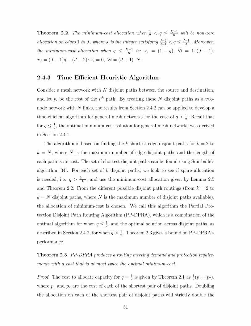
Theorem 2.2. The minimum-cost allocation when 12< q ≤ K−1

Kwill be non-zero

allocation on edges 1 to J , where J is the integer satisfying J−2J−1 < q ≤ J−1

J. Moreover,

the minimum-cost allocation when q ≤ K−1K

is: xi = (1 − q), ∀i = 1..(J − 1);

xJ = (J − 1)q − (J − 2); xi = 0, ∀i = (J + 1)..N .

2.4.3 Time-Efficient Heuristic Algorithm

Consider a mesh network with N disjoint paths between the source and destination,

and let pi be the cost of the ith path. By treating these N disjoint paths as a two-

node network with N links, the results from Section 2.4.2 can be applied to develop a

time-efficient algorithm for general mesh networks for the case of q > 12. Recall that

for q ≤ 12, the optimal minimum-cost solution for general mesh networks was derived

in Section 2.4.1.

The algorithm is based on finding the k-shortest edge-disjoint paths for k = 2 to

k = N , where N is the maximum number of edge-disjoint paths and the length of

each path is its cost. The set of shortest disjoint paths can be found using Suurballe’s

algorithm [34]. For each set of k disjoint paths, we look to see if spare allocation

is needed, i.e. q > k−1k

, and use the minimum-cost allocation given by Lemma 2.5

and Theorem 2.2. From the different possible disjoint path routings (from k = 2 to

k = N disjoint paths, where N is the maximum number of disjoint paths available),

the allocation of minimum-cost is chosen. We call this algorithm the Partial Pro-

tection Disjoint Path Routing Algorithm (PP-DPRA), which is a combination of the

optimal algorithm for when q ≤ 12, and the optimal solution across disjoint paths, as

described in Section 2.4.2, for when q > 12. Theorem 2.3 gives a bound on PP-DPRA’s

performance.

Theorem 2.3. PP-DPRA produces a routing meeting demand and protection require-

ments with a cost that is at most twice the optimal minimum-cost.

Proof. The cost to allocate capacity for q = 12

is given by Theorem 2.1 as 12(p1 + p2),

where p1 and p2 are the cost of each of the shortest pair of disjoint paths. Doubling

the allocation on each of the shortest pair of disjoint paths will strictly double the

51

10

15

20

25

30

35

0 0.1 0.2 0.3 0.4 0.5 0.6 0.7 0.8 0.9 1

Cos

t

q

1+1 1+q PP-DPRA LP PP

Figure 2-8: Algorithm comparison: cost vs. q

total cost. We note that this allocation is sufficient to provide protection for all q ≤ 1;

so the cost for protecting all q ≤ 1 using a pair of disjoint paths is at most double that

of q = 12. The minimum-cost to provide protection is monotonically non-decreasing

with respect to the value of the partial protection requirement q; this can be clearly

seen because if there existed a solution for a demand for some q2 that has a lower

cost than that of some q1, where q2 > q1, then the solution for q2 would be used

to protect for q1 as well. Since the optimal solution is monotonically non-decreasing

with respect to q, we know that routing 12

unit of flow onto each of the shortest pair

of disjoint paths is a lower bound, and routing 1 unit of flow onto each of the disjoint

paths will be an upper bound. Hence, routing onto the shortest pair of disjoint paths

is at most twice the cost of the optimal solution for any q > 12. Using more disjoint

paths, if possible, can only lower the total cost needed to meet demand and protection

requirements.

To assess PP-DPRA’s performance, PP-DPRA is compared to 1 + 1, 1 + q, and

LPPP . The simulation is similar to the one run in Section 2.3.2 for the case when

backup capacity sharing is not possible. PP-DPRA is implemented in C. The average

52

costs to meet demand and protection requirements over all random graphs are plotted

in Figure 2-8. Simulation results show that for q ≤ 12, as anticipated, the routing

given by Theorem 2.1 matches the optimal routing produced by LPPP . For q >

12, the average cost is greater than the minimum-cost solution by 1.4% on average.

Additionally, on average, the running time for routing a demand with PP-DPRA was

10−3 seconds, while with the linear program LPPP it was 22 seconds. This reduction

in running time of four orders of magnitude makes the algorithm suitable for networks

that require rapid setup times for incoming demands.

2.5 Solutions with Backup Capacity Sharing

In Section 2.3, a linear program that finds the minimum-cost solution for the partial

protection problem utilizing backup capacity sharing was presented. A linear program

is often not an efficient method of finding a solution, and in Section 2.4, an efficient

algorithm was presented for the case without backup capacity sharing. These results

offer a fundamental understanding of the partial protection problem, and are useful

for networks that do not allow protection sharing. But often, networks do utilize

backup sharing, and significant savings can often be achieved. In this section, a

time-efficient algorithm for partial protection in general mesh networks using backup

capacity sharing is presented.

If two primary flows for two different demands are edge-disjoint from one another,

then under a single-link failure model, at most one can be disrupted at any given

point in time. Since at most one demand will need to be restored after a failure, two

failure-disjoint flows can share backup capacity.

Determining how much backup capacity can be shared for 1+1 guaranteed protec-

tion was investigated in [18, 19]. They consider the case of dynamic (one-at-a-time)

arrivals, and we use a similar model for the development of our algorithm. In those

papers, conflict sets were used to determine potential backup sharing on an edge by

examining of how much backup capacity was allocated on one edge to protect against

the failure of another. If more backup capacity is already allocated than is needed on

53

some edge to protect for the failure of another edge, then that edge’s backup capacity

can be shared. This model can be extended to partial protection by guaranteeing

that any particular demand has its partial flow requirement met after a failure.

For the case of one-at-a-time routing, previous works offer heuristics to jointly

optimize the primary and backup path for each incoming demand, as was done in

[18, 19]. We instead choose a simple strategy of using the shortest path for the

primary route. Our simulations show that using the shortest path for the primary

route in fact performs better than jointly optimizing the primary and backup paths

for each incoming demand. We call our algorithm Dynamic Shared Partial Protection

(DSPP).

We compare, via simulation, DSPP to 1 + 1, 1 + q and the non-preemptive LP

(LPPP ), each of which jointly optimizes the primary and backup paths for each in-

coming demand (a “greedy optimal” approach). Demands arrive dynamically and

are served one-at-a-time in the order of their arrival. Performance of the strategies

is compared using the NSFNET topology (Fig. 2-6) with 100 random unit demands.

The protection requirement, q, for each demand has a truncated normal distribution

with a standard deviation σ = 12. The mean of q is varied between 0 and 1 for each

iteration.

The costs to route the demand and protection capacity are plotted in Fig. 2-9 as a

function of the expected value of q. It is seen that when demands are routed one at a

time with a greedy optimal approach, the partial protection scheme offers significant

savings over 1 + 1 routing over a wide range of q, with LPPP achieving even greater

gains than 1 + q protection because of its use of flow bifurcation. With dynamic

arrivals, we find that DSPP performs better than the greedy schemes that jointly

optimize the primary and backup paths. The greedy optimal approach of jointly

optimizing the primary and backup routes will often take a longer primary path

for an incoming demand in order to take advantage of backup sharing. The longer

primary path makes it more difficult for future demands to find disjoint primary

routes, thus lowering their ability to share protection resources. While other works

have focused on finding heuristics to jointly optimize the primary and backup paths

54

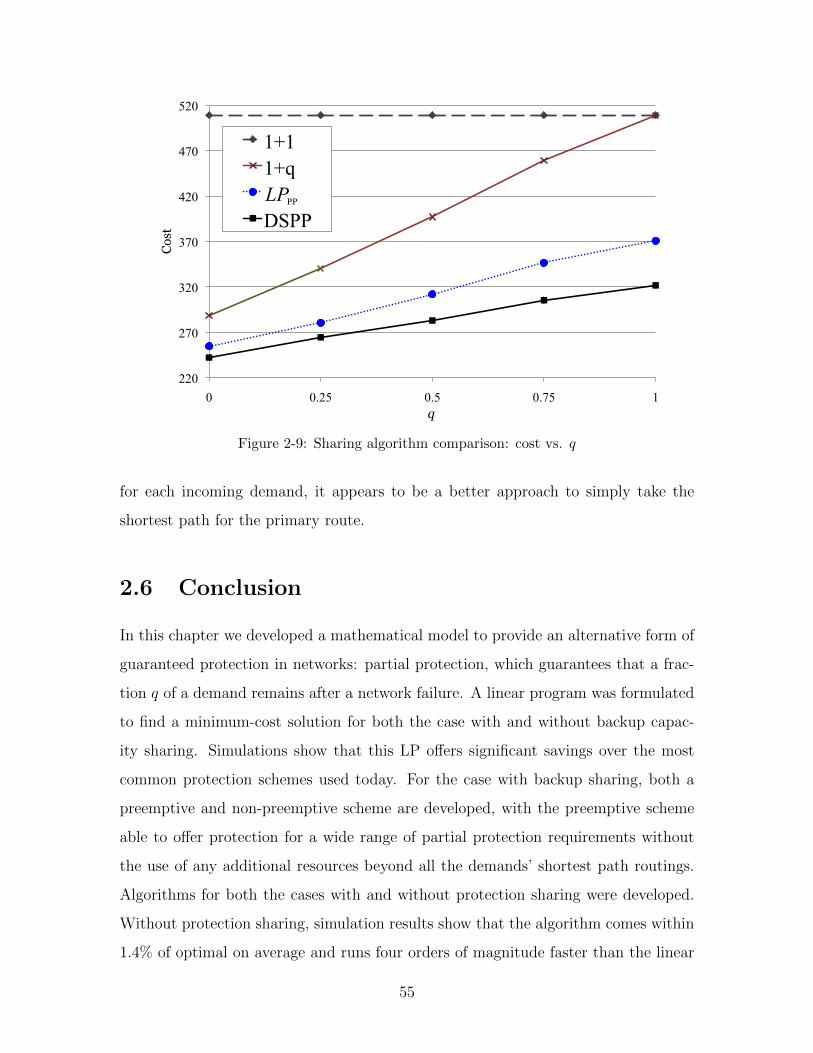
220

270

320

370

420

470

520

0 0.25 0.5 0.75 1

Cos

t

q

1+1 1+q LP DSPP

PP

Figure 2-9: Sharing algorithm comparison: cost vs. q

for each incoming demand, it appears to be a better approach to simply take the

shortest path for the primary route.

2.6 Conclusion

In this chapter we developed a mathematical model to provide an alternative form of

guaranteed protection in networks: partial protection, which guarantees that a frac-

tion q of a demand remains after a network failure. A linear program was formulated

to find a minimum-cost solution for both the case with and without backup capac-

ity sharing. Simulations show that this LP offers significant savings over the most

common protection schemes used today. For the case with backup sharing, both a

preemptive and non-preemptive scheme are developed, with the preemptive scheme

able to offer protection for a wide range of partial protection requirements without

the use of any additional resources beyond all the demands’ shortest path routings.

Algorithms for both the cases with and without protection sharing were developed.

Without protection sharing, simulation results show that the algorithm comes within

1.4% of optimal on average and runs four orders of magnitude faster than the linear

55

program. For the case with protection sharing, the algorithm developed actually per-

forms better than jointly optimizing the primary and backup paths for each incoming

demand.

2.7 Chapter Appendix

2.7.1 Proofs for Section 2.4.1

Proof of Lemma 2.1. First we show that if there is no spare capacity on any link, i.e.

sij = 0, ∀{i, j} ∈ E, and all flow and protection requirements are satisfied, then it

must be the case that xij ≤ (1−q), ∀{i, j} ∈ E. Assume all requirements are satisfied,

and that there exists an edge {k, l} such that xkl > (1− q) with sij = 0, ∀{i, j} ∈ E.

After the failure of {k, l}, less than q of the flow will remain between the source and

destination, which is below the partial protection requirement of q. This implies spare

allocation on some edge will be needed to meet all requirements, which contradicts

our original assumption.

We now consider the other direction: if xij ≤ (1 − q), ∀{i, j} ∈ E, then the

required spare capacity is zero on all edges: sij = 0, ∀{i, j} ∈ E. This is straightfor-

ward to see since after the failure of any edge, at most (1 − q) of flow between the

source and destination is disrupted, leaving at least q, which meets parital protection

requirements.

Proof of Lemma 2.2. For some q ≤ 12, assume there exists a minimum-cost solution

with an edge {i, j} that has sij > 0. Since a minimum-cost solution has an edge with

spare capacity allocated to it, according to Lemma 2.1, there must exist some edge

{k, l} with primary capacity allocation greater than (1−q), i.e. xkl = 1−q+ε, ε > 0.

To meet protection requirements, after the failure of edge {k, l}, the remaining

flows between s and t must have a total capacity of q. The amount of primary flow

remaining after the failure of the edge carrying (1 − q + ε) is (q − ε), which means

that at least ε flow of spare allocation will be necessary along some of the protection

paths. If this spare allocation was instead used as primary traffic, the primary flow

56

on {k, l} would decrease from 1− q+ ε to 1− q, which by Lemma 2.1 implies that no

spare allocation is necessary. This maintains the total flow from s to t at 1; hence,

the primary demand and protection requirements are met. Clearly, the total cost

of the allocation without spare capacity is less than the cost with spare since the

primary capacity on {k, l} is reduced and the spare allocation on edge {i, j} can be

removed.

Proof of Theorem 2.1. The modified linear program LPq≤.5 seeks to find a minimum-

cost routing with capacitated edges. This is recognized to be a minimum-cost flow

formulation, which is defined as finding a flow of lowest cost between a source and

destination in a network that has both edge costs and edge capacities [29]. Algo-

rithms exist for finding optimal solutions to minimum-cost flow problems. One such

algorithm is the successive shortest paths (SSP), which successively finds the shortest

path and routes the maximum flow possible on that path [29]. This is repeatedly

done until the desired flow between the source and destination is routed. After SSP

terminates, a set of edge allocations representing the minimum-cost flow will be re-

turned. The paths that these edges represent, and those paths’ respective flows, can

be found by using the path decomposition algorithm [29].

Before we specify the details of SSP, we first define a residual graph, which is

commonly used in maximum flow algorithms [29]. If edge {i, j} has a capacity and

cost of (uij, cij) in a graph G with a flow of xij ≤ uij on it, then the residual graph Gr

will have two edges {i, j}r and {j, i}r with respective costs and capacities (uij − xij,

cij), and (xij, −cij). Any flow in a residual graph preserves all node conservation

constraints in the original graph [29].

The successive shortest paths algorithm is as follows: for a total demand of d

needing to be routed from node s to t, first find the shortest path and route flow

equal to the lowest capacity edge in that path. If the limiting edge has capacity u∗,

then d − u∗ remains to be routed (assuming that d > u∗). Next, a residual graph

is created from the allocation routed on the shortest path. To route the remaining

d − u∗ of flow, the shortest path in the newly formed residual graph is found. If

d− u∗ is less than the lowest capacity edge in that path, the algorithm is completed

57

by routing the remaining d− u∗ flow from s to t. Otherwise, flow equal to the lowest

capacity edge in shortest path from s to t is routed, the residual graph is updated,

and the process is repeated until all of the required d flow has been routed.

In our original network G, every edge has capacity (1 − q); hence, the lowest

capacity edge in any path is (1 − q). We find the shortest path in G, with a set of

edges E0 and having a total cost p0; (1− q) of flow is routed on the set of edges E0.

In the residual graph, each edge {i, j} ∈ E0 no longer has capacity and is removed,

and a new set of edges Er0 = {{j, i}r : {i, j} ∈ E0} is added, with each edge having

capacity (1 − q). All other edges that were not part of the shortest path remain in

the residual graph with a capacity of (1− q). Since (1− q) was routed on the shortest

path, a flow of q remains to be routed from s to t in the residual graph. All of the

edges in the residual graph have a capacity of (1 − q), and since we assume q ≤ 12,

we know that q ≤ (1 − q). Hence, the next shortest path from s to t in the residual

graph, with the set of edges E1 and having a total cost of p1, has sufficient capacity

to satisfy the q amount of remaining flow that needs to be routed.

Two cases are possible: (1) if the second path does not use edges created in the

residual graph by the initial shortest path, i.e. E1 ∩ Er0 = ∅, and (2) if the second

path does use those edges, i.e. E1 ∩ Er0 6= ∅.

For case 1, the first and second path do not overlap, and hence happen to be the

shortest pair of disjoint paths in the network between s and t. Since (1 − q) was

routed onto the first shortest path, and q routed onto the next shortest disjoint path,

we have the same flow as if routing (1−2q) onto the shortest path, and q onto each of

the shortest pair of disjoint paths. This yields a total allocation cost of p0(1−q)+p1q.

For case 2, the set of edges {j, i}r ∈ E1∩Er0 those edges where the second shortest

path in the residual graph overlaps with the initial shortest path that was found in the

original graph. Any allocation on {j, i}r ∈ E1 ∩ Er0 “cancels” original flow allocated

on edge {i, j} from the first shortest path found, i.e., if 1 unit of flow is routed on edge

{i, j} in the original graph, and 12

unit of flow is allocated on {j, i}r in the residual

graph, then the flow in the original graph on edge {i, j} is 12. The flow on the edges

where the two paths overlapped is xij = (1−q)−q = (1−2q), ∀{j, i} ∈ E1∩Er0 , which

58

is non-negative since q ≤ (1− q). The remaining edges that did not overlap maintain

their original flow values: if {i, j} belonged to E0, then it’s value is xij = (1− q), and

if {i, j} belonged to E1, then it’s value is xij = q.

To recover the paths, we use flow decomposition [29], which is to repeatedly find

a path from source to destination, and subtract the flow equivalent to the minimum

edge capacity until all flow from the network has been assigned to some path (almost

a successive shortest paths in reverse). We first find the edges of the shortest path,

which now has a maximum flow of (1 − 2q). After removing this flow from the

network, we are left with two disjoint paths of q flow each, and costs of p1 and p2,

respectively. These disjoint paths are by definition the minimum-cost pair of disjoint

paths: if there existed a lower cost pair of disjoint paths, then we can produce a

lower cost flow by routing (1 − 2q) onto the shortest path and q onto each of the

lower cost pair of disjoint paths, which is a feasible flow and would give a lower cost

routing, which is not possible since the successive shortest paths algorithm found the

minimum-cost solution. Hence, we are left with a minimum-cost solution having a

cost of (1− 2q)p0 + q(p1 + p2).

2.7.2 Proofs of Section 2.4.2

The following is used throughout all proofs in this section: AN is the N x N matrix

of 1’s with the identity matrix subtracted from it (an all 1’s matrix with a diago-

nal of zeros), cN and xN are the cost and edge allocation row vectors for N edges,

respectively, and eN is a column vector of N 1’s. The expression C = [A B] de-

notes a concatenation of matrices A and B. Throughout these proofs, results from

optimization theory are used, with pertinent details being found in [28].

We note that first the proofs for Lemmas 2.4, 2.5, and 2.6 are given before the

proof for Lemma 2.3.

Proof of Lemma 2.4. For a given set of edges E with the ith edge having a cost of ci,

the linear program for a two-node network needing to route a unit-demand with a

59

partial protection requirement of q can be written as follows:

LP2 : min x′NcN (2.11)

s.t. ANxN ≥ qeN (2.12)∑i∈E

xi ≥ 1 (2.13)

xi ≥ 0, ∀i ∈ E (2.14)

Constraint 2.13 specifies that at least one unit of flow must be routed across the

set of links, and Constraint 2.12 indicates that after any particular link fails, at least

q flow must remain across the remaining set of links.

Since we assume that spare allocation is needed, the total allocation across the

set of edges is strictly greater than 1. Hence, Constraint 2.13, which indicates that

flow must be at least 1, is not tight, and can be disregarded.

When solving the primal, LP2, we know generally that some K ≤ N edges are

active, and N −K edges are not, i.e. if edge i is active, then xi > 0, and vis versa.

We note again that the solution will clearly use the K lowest cost edges, otherwise

capacity can be shifted from higher to lower cost edges, yielding a lower cost solution.

With the K lowest cost variables being active, and the N −K highest cost variables

being zero, constraints K + 1 through N all have the form∑K

i=1 xi ≥ q. Summing

the first K constraints, we find∑K

i=1 xi = q KK−1 ; constraints K + 1 through N are all

clearly no longer active (and they also no longer linearly independent), and they can

be disregarded. By removing the constraints from LP2 that are not tight, we are left

with K variables and K constraints. To solve for K variables, all K constraints must

be used, and can be set to equality. The primal is rewritten as follows:

LP2K : min x′KcK (2.15)

s.t. AKxK = qeK (2.16)

xi ≥ 0, ∀i = 1..K (2.17)

60

This solution is straightforward to find, and is an even distribution of xi = q 1K−1 , ∀i =

1..K.

We now use an inductive approach to show that all edges that satisfy the re-

quirement cj <1

K−1∑K

i=1 ci are in fact part of the minimum-cost solution, where

K = argmaxK=2..N(cK ≤ 1K−1

∑Ki=1 ci). Assume that a minimum-cost solution uses

the J − 1 lowest cost edges, and that the J th edge has cost cJ < 1J−1

∑Ji=1 ci. If

J − 1 edges are used, then as shown above, the solution will be an even distribution

across those J − 1 edges of xi = q 1J−2 , ∀i = 1..(J − 1). The total cost of the assumed

optimal solution is q 1J−2

∑J−1i=1 ci. We now consider the solution that uses edge J ,

which was previously excluded. With J edges being used, each edge will have an

even allocation of xi = q 1J−1 , ∀i = 1..J , and the total cost across the J edges will

be q 1J−1

∑Ji=1 ci. Using some algebraic manipulation, we see that the solution using

J edges will have higher cost only if cJ >1

J−1∑J

i=1 ci, but we assumed otherwise.

Hence, a lower-cost solution can be obtained if all J edges are used. Inductively, we

see that this approach can be continued until we find the K lowest-cost edges such

that K = argmaxK=2..N(cK ≤ 1K−1

∑Ki=1 ci).

Proof of Corollary ??. The set of K edges that are active in a minimum cost so-

lution when spare capacity is needed is given by the result in Lemma 2.4: K =

argmaxK=2..N(cK ≤ 1K−1

∑Ki=1 ci), which does not depend on q.

Proof of Lemma 2.5. In the proof for Lemma 2.4, a solution that optimally solved the

two-node network was found for the primal formulation LP2K , which uses K edges, by

setting the the constraints to equality. This solution was an even distribution of xi =

q 1K−1 , ∀i = 1..K. We can perform an additional check that our solution is optimal

by verifying complementary slackness conditions (not done here for brevity).

Proof of Lemma 2.6. When spare allocation is not needed, the total allocation across

61

all of the edges is 1.

LP2 : min c′NxN (2.18)

s.t. ANxN ≥ qe′N (2.19)

N∑i=1

xi = 1 (2.20)

xi ≥ 0, ∀i ∈ E (2.21)

The corresponding dual is as follows:

LP2d : max∑i=1..N

qpi + pN+1 (2.22)

s.t. p′N+1[AN eN] ≤ c′N (2.23)

pi ≥ 0, ∀i = 1..(N + 1) (2.24)

We note that the dual variable, pN+1, corresponding to the primal constraint∑i=1..N xi = 1, is no longer necessarily zero, as it would be if

∑i=1..N xi > 1.

We initially find an optimal solution to the problem as if it requires spare capacity,

which assumes Constraint 2.20 is not active. When Constraint 2.20 is set to equality,

then the current solution is still dual feasible if pN+1 is set to zero. The solution with

spare capacity (given in Lemma 2.5) uses an even distribution of q 1K−1 on each of

the K lowest cost edges, where K = argmaxK=2..N(cK ≤ 1K−1

∑Ki=1 ci). Since the

K lowest cost edges are used, then the first K constraints will be active in the dual.

Additionally, since the first K constraints are tight in LP2, the first K dual variables

will be used to solve for an optimal dual solution. Hence, the solution to the dual

will have pi > 0, ∀i = 1..K, and pi = 0, ∀i = (K + 1)..N .

We now consider the case when spare capacity is not used. The solution for when

spare capacity is used remains dual feasible when the spare allocation is not used

if pN+1 is initially set to 0. This solution, while being feasible, is not necessarily

optimal. We will use this initial dual feasible solution as our starting point. The

initial dual feasible solution has the first K constraints tight (at equality); each of

62

these constraints contain the variables pK+1 to pN+1, which are all initially equal to

zero.

We wish to find a lower cost solution to the primal, which means finding a higher

value for the objective of the dual. Due to the structure of the problem’s linear

program and its subsequent dual, if any dual variable pi, i = 1..N , has value greater

than zero, then the corresponding edge i (primal variable xi) will be non-zero. We

wish to show that when a solution does not use spare capacty, that at most the K

lowest cost edges will be used, where the K edges are those used for the minimum-cost

allocation when spare allocation is needed. Hence, we want to show that raising the

value of any dual variable pK+1 through pN will not raise the objective function. In

the current dual feasible solution, where pN+1 is set to zero, all constraints 1 through

K are tight. To increase the value of any dual variable that is currently at zero

(pK+1 through pN+1), the sum of the dual variables that currently have value must

be decreased.

Assume we wish to raise pK+1 through pN+1 by some amount δ, i.e.∑N+1

i=K+1 pi = δ.

Since the first K constraints are tight, we must decrease p1 to pK by at least δ.

Consider the jth tight constraint for some j ≤ K. The jth constraint has the following

form: p1 + p2 + ... + 0pj + ... + pK +∑N+1

i=K+1 pi = cj, where pj is multiplied by zero

to show that it does not appear in the jth constraint. To raise∑N+1

i=K+1 pi by δ, the

K − 1 dual variables that are greater than zero in the jth constraint must each be

reduced by 1K−1δ. When we consider all K tight constraints, it can be easily shown

that the only feasible solution to raise∑N+1

i=K+1 pi by δ is to lower each dual variable

p1 through pK by 1K−1δ. Hence, to achieve the increase of δ across the variables pK+1

through pN+1, the total decrease across the first K dual variables is KK−1δ, which we

note is greater than δ.

Looking at the objective function (Equation 2.22), it can be seen that dual vari-

ables p1 through pN all have the same cost of q. Any increase in the dual variables

pK+1 through pN will result in a larger decrease of the dual variables p1 through pK ,

which will bring down the total value of the objective. Hence, raising the value of

pK+1 through pN will not find a new maximum for the objective. The cost of the dual

63

variable pN+1 in the objective is 1, and q ≤ 1. So, it may be possible to raise pN+1

while decreasing p1 throught pK , and also increase the objective function. The dual

variable pN+1 appears in each of the first K tight constraints. Again, consider the

jth tight constraint for some j ≤ K, and exclude the dual variables pK+1 through pN .

The jth constraint has the following form: p1 + p2 + ... + 0pj + ... + pK + pN+1 = cj.

Raising pN+1 will simply result in a strict decrease across the first K dual variables.

Furthermore, since pK+1 through pN also appear in each of the first K tight con-

straints, there is never a reason to raise some pi, (K + 1) ≤ i ≤ N , since a larger

increase in the objective can be achieved by shifting any allocation that would go to

pi to pN+1 instead. Hence, if pN+1 were raised, at most the original dual variables p1

through pK will be non-zero, which will yield a solution using at most the K lowest

cost edges.

Proof of Lemma 2.3. First, assume there exists a minimum-cost solution that uses

spare capacity when q ≤ K−1K

. Since we assume that spare capacity is used for a

minimum-cost solution, we know that the results from Lemmas 2.4 and 2.5 hold.

The total capacity allocated for a minimum-cost solution across the K links is q KK−1 .

Since we assumed that q ≤ K−1K

, the total allocation across all of the links is q KK−1 ≤

K−1K

KK−1 = 1, which means that the total allocation either uses no spare allocation or

is insufficient to meet the primary demand. Hence, we have a contradiction.

Next, assume there exists a minimum-cost solution using no spare capacity if

q > K−1K

. Continuing the proof from Lemma 2.5, we consider the objective function

of the dual, max∑

i=1..N qpi + pN+1. If the dual variable pN+1 is greater than zero,

then its corresponding primal constraint (Constraint 2.20) must be tight (by way of

complementary slackness). If Constraint 2.20 is tight, then no spare allocation is used.

In the proof for Lemma 2.5, a dual feasible solution was considered, and the conditions

for increasing the objective were found. To increase the dual variable pN+1 by δ, the

first K dual variables must be decreased by a total of δ KK−1 . The cost of each of the

first K dual variables is q, while the cost of pN+1 is 1. The dual objective can only be

raised if the decrease in cost from lowering the first K dual variables is offset by an

even larger increase in the objective by raising pN+1. A δ increase in pN+1 increases

64

the objective by δ, but decreases the first K dual variables by δ KK−1 , which lowers

the objective by qδ KK−1 . We assume that q > K−1

K. The decrease in the objective

from the first K dual variables is qδ KK−1 > δK−1

KKK−1 > δ. Hence, when q > K−1

K, a

better solution can be found by having pN+1 be greater than zero, which means that

no spare allocation is used, thus contradicting our original assumption.

Proof of Theorem 2.2. We continue the proof from Lemma 2.3. As was shown, when

q ≤ K−1K

, the objective of the dual function can be raised by increasing pN+1. The

initial dual feasible solution when q < K−1K

has p−N + 1 set to zero. Solving for the

dual variables in the set of linear equations of our initial solution (while pN+1 is at

0), we get pj =∑K

i=1 ci −2K−3K−1 cj. By definition, c1 ≤ c2 ≤ ... ≤ cN , so the solution

to the dual variables are pK ≤ pK−1 ≤ ... ≤ p1. To increase pN+1 by some value δ, p1

to pK each decrease by δ 1K−1 , for a total decrease of δ K

K−1 .

We now increase δ by increments, until one of the dual variables goes to zero.

Since each dual variable decreases by the same amount δ 1K−1 , the dual variable with

the lowest value will go to zero first. The dual variable pK will be the first to go

to zero, and the corresponding Kth constraint is no longer active, giving a solution

where the Kth edge has zero allocation; this was the most expensive edge that was

in use, so it matches intuition that it would be the first to go to zero. Currently, p1

to pK−1 are greater than zero, and pN+1 is also greater than zero. We wish to see if

we can further increase pN+1 and continue raising the objective value. Without pK ,

which is now zero, we have the following objective function: max∑K−1

i=1 qpi + pN+1.

Using a similar process as above, we get the condition that we will increase δ (which

is pN+1) only if q < K−2K−1 . This process can be repeated until raising the value of pN+1

further does not increase the objective. Inductively, we stop increasing pN+1 when

we have J active dual variables such that J−1J−2 < q ≤ J

J−1 , where J is an integer. By

complementary slackness, there are J active constraints in the primal, which yields a

solution using J variables, which will be the J lowest cost edges. We get the following

set of J independent equations: x′J[AJ−1 eJ] = [qeJ 1]′. We can solve this set of linear

equations, and obtain the results in Theorem 2.2.

65

Chapter 3

Protection with Multiple

Availability Guarantees

3.1 Introduction

In Chapter 2, we considered providing protection that guarantees a minimum-grade of

service after a failure, which we termed “partial protection”. This partial protection

scheme offered significant savings over the full protection scheme, but it allowed flow

to drop to its lower grade of service after any link failure that disrupted service.

An alternative approach is to provide a guarantee on the maximum time a con-

nection can be disrupted. This is known as an “availability guarantee”, and it is a

bound on the fraction of time or probability that a connection can be disrupted. How-

ever, these disruptions (downtimes) may be unacceptably long; thus, many service

providers opt for the more resource intensive full protection. In this chapter, we pro-

pose a novel protection scheme with multiple availability guarantees. In addition to

the traditional availability guaranteed protection, which maintains the full demand

for at least a guaranteed fraction of time, we guarantee partial connectivity at all

times (similar to the partial protection scheme of Chapter 2). Thus, our approach is

a hybrid between the traditional availability guarantees and full protection schemes.

Full protection schemes have been studied extensively [2, 4, 5, 17–19, 46]. The

most common scheme in backbone networks today is 1+1 guaranteed path protection

67

[3], which provides an edge-disjoint backup path for each working path, and guaran-

tees the full demand to be available at all times after any single link failure. There

has also been a growing body of literature for backup provisioning to meet availability

guarantees [47–53]. In all of these, primary and backup flows are allocated such that

the connection is disrupted for at most a specified fraction of time or probability. Dur-

ing these down-states, the service is completely disrupted. A version of availability

guarantees is considered in [54], where an end-to-end flow having a certain expected

capacity, based on link availabilities, is found; no guarantees on flow are provided.

In this chapter, a flow is guaranteed to be at least a fraction q of the full demand

at all times, which is known as “partial protection”. Our novel approach is the first

to combine the traditional availability guarantee and partial protection guarantee to

allow the user to specify flows with different availability guarantees. Moreover, it is

particularly applicable to IP-over-WDM networks where MPLS tunnels are used to

provision resources.

The partial protection framework was first introduced in [42]. In Chapter 2, we

developed a “theory” of partial protection such that after any single link failure, the

flow can drop to the partial protection requirement. In Chapter 2, a fraction q of the

demand is guaranteed to remain available between the source and destination after

any single link failure, where q is between 0 and 1. When q is equal to 1, the service

will have no disruptions after any single failure, and when q is 0, there will be no flow

between the two nodes during the down state. In our work, flows can drop below the

full demand for at most a specified fraction of time, and maintain at least q of that

demand at all times. Similar to [49–53], the probability of simultaneous failures is

assumed to be negligible and we only consider single-link failures.

The novel contributions of this chapter include a framework for Multiple Avail-

ability Guaranteed Protection (MAGP) and providing associated algorithms for both

the cases when protection resources can and cannot be shared. Moreover, in the q = 0

case, corresponding to the previously studied scenario where full availability is guar-

anteed for a fraction of time, we develop an optimal pseudo-polynomial algorithm.

This chapter is outlined as follows. In Section 3.2, the model for MAGP is de-

68

scribed. In Section 3.3, MAGP is shown to be NP-Hard, and the minimum-cost

solution to MAGP is formulated as an MILP. In Section 3.4, optimal solutions and

algorithms for MAGP are developed when protection resources cannot be shared, and

in Section 3.5, an algorithm is developed for when protection resources can be shared.

3.2 Multiple Availability Guaranteed Protection

In this chapter, routing strategies are developed and analyzed to minimize the total

cost and capacity allocation required to satisfy each demand’s protection and avail-

ability requirements. A demand needs to be routed from its source s to destination t

such that the flow can drop below the full demand for at most some specified down-

time, and maintain at least a fraction q of that full demand at all times. To simplify

the analysis, a “snapshot” model is used: the network state is considered after a fail-

ure has occurred. Let pij be the conditional probability that edge {i, j} failed given

that a network failure has occurred. For ease of exposition, instead of a maximum

downtime, the Maximum Failure Probability (MFP) is considered, and its value is

denoted by P . After some network failure, the flow can be below the full demand,

but at least a fraction q of the demand, with at most probability P . The maximum

failure probability is the conditional probability that the network is in a downstate

given some link disruption. This value can be easily related to the maximum down-

time by accounting for expected time between failures and mean time to repair (e.g.,

see [54]).

We assume that the graph G, with a set of vertices V , edges E, and edge failure

probabilities P , is at least two-connected. Since only single-link failures are con-

sidered, edge failures are disjoint events, which gives∑{i,j}∈E pij = 1. Similar to

previous works, the primary flow is restricted to a single path. After the failure

of a link, a network management algorithm reroutes the traffic along the allocated

protection paths.

Consider the example in Fig. 3-1, with link failure probabilities and flow alloca-

tions as labeled (p and f respctively). A unit demand needs to be routed from s to

69

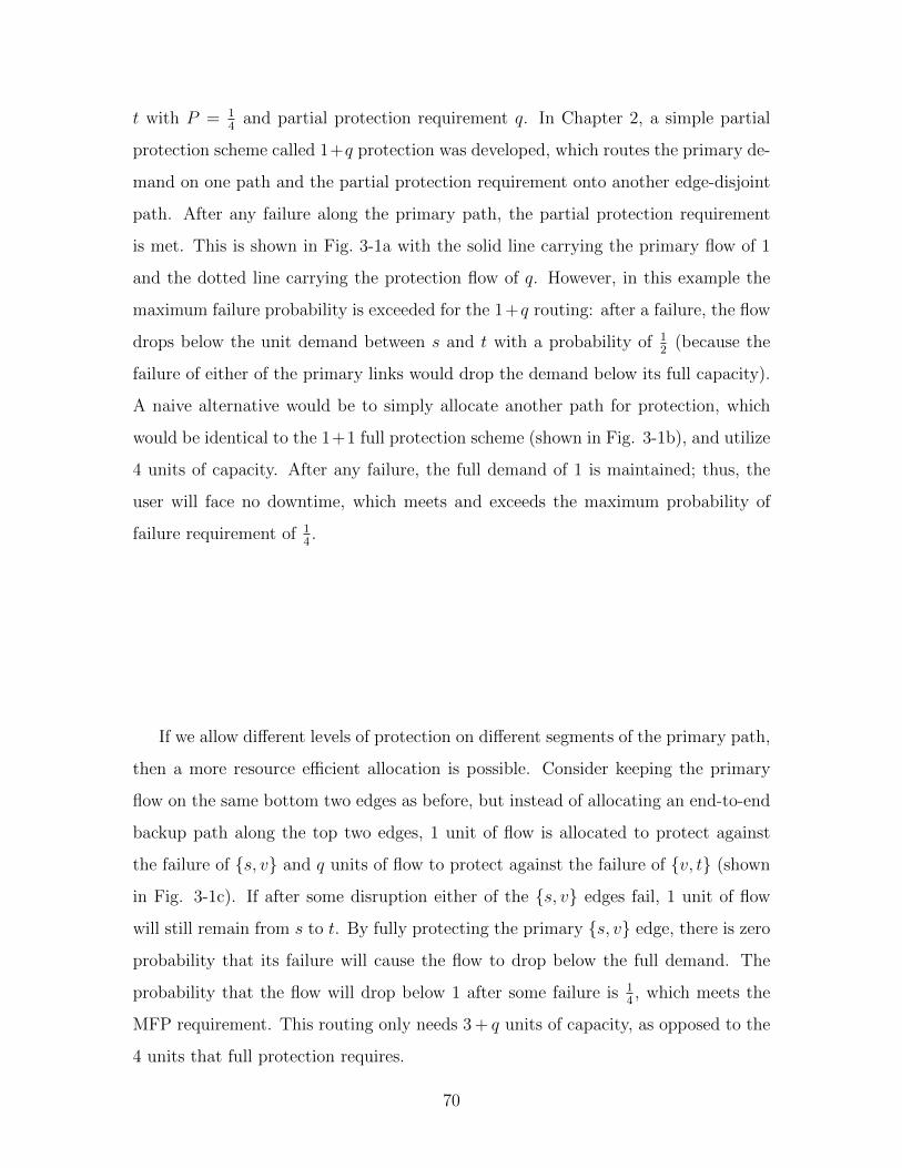
t with P = 14

and partial protection requirement q. In Chapter 2, a simple partial

protection scheme called 1+q protection was developed, which routes the primary de-

mand on one path and the partial protection requirement onto another edge-disjoint

path. After any failure along the primary path, the partial protection requirement

is met. This is shown in Fig. 3-1a with the solid line carrying the primary flow of 1

and the dotted line carrying the protection flow of q. However, in this example the

maximum failure probability is exceeded for the 1+q routing: after a failure, the flow

drops below the unit demand between s and t with a probability of 12

(because the

failure of either of the primary links would drop the demand below its full capacity).

A naive alternative would be to simply allocate another path for protection, which

would be identical to the 1+1 full protection scheme (shown in Fig. 3-1b), and utilize

4 units of capacity. After any failure, the full demand of 1 is maintained; thus, the

user will face no downtime, which meets and exceeds the maximum probability of

failure requirement of 14.

If we allow different levels of protection on different segments of the primary path,

then a more resource efficient allocation is possible. Consider keeping the primary

flow on the same bottom two edges as before, but instead of allocating an end-to-end

backup path along the top two edges, 1 unit of flow is allocated to protect against

the failure of {s, v} and q units of flow to protect against the failure of {v, t} (shown

in Fig. 3-1c). If after some disruption either of the {s, v} edges fail, 1 unit of flow

will still remain from s to t. By fully protecting the primary {s, v} edge, there is zero

probability that its failure will cause the flow to drop below the full demand. The

probability that the flow will drop below 1 after some failure is 14, which meets the

MFP requirement. This routing only needs 3 + q units of capacity, as opposed to the

4 units that full protection requires.

70

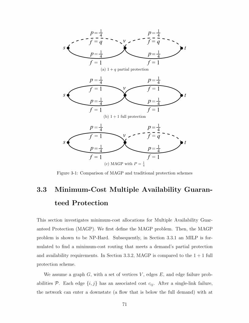
(a) 1 + q partial protection

(b) 1 + 1 full protection

(c) MAGP with P = 14

Figure 3-1: Comparison of MAGP and traditional protection schemes

3.3 Minimum-Cost Multiple Availability Guaran-

teed Protection

This section investigates minimum-cost allocations for Multiple Availability Guar-

anteed Protection (MAGP). We first define the MAGP problem. Then, the MAGP

problem is shown to be NP-Hard. Subsequently, in Section 3.3.1 an MILP is for-

mulated to find a minimum-cost routing that meets a demand’s partial protection

and availability requirements. In Section 3.3.2, MAGP is compared to the 1 + 1 full

protection scheme.

We assume a graph G, with a set of vertices V , edges E, and edge failure prob-

abilities P . Each edge {i, j} has an associated cost cij. After a single-link failure,

the network can enter a downstate (a flow that is below the full demand) with at

71

most a Maximum Failure Probability (MFP) of P , where the MFP is the conditional

probability that the network is in a downstate given some link disruption. During a

downstate, the flow between a source and destination may fall below the full demand,

but must always remain at a minimum guaranteed fraction q of the demand. We now

show that finding the minimum-cost solution to MAGP is NP-Hard.

Theorem 3.1. The Minimum-cost Multiple Availability Guaranteed Protection prob-

lem is NP-Hard.

Proof. To demonstrate NP-Hardness of MAGP, a reduction from the 1-0 knapsack

problem [37] is performed. See Chapter Appendix Section 3.7.1 for the complete

proof.

3.3.1 Mixed Integer Linear Program to Meet Multiple Avail-

ability Guaranteed Protection

Since finding a minimum-cost solution for MAGP is NP-Hard, in this section a mixed

integer linear program (MILP) is developed to solve for the minimum-cost solution.

For a connection request between two nodes s and t, the flow can drop to a fraction

q of the demand with at most probability P . Again, the snapshot model is used,

and the set of link failure probabilities P are conditional given a network failure has

occurred.

For the MILP, the following values are given:

• G = (V,E,C,P) is the graph with its set of vertices, edges, costs, and edge

failure probabilities, respectively

• dst is the required demand between nodes s and t

• qst is the fraction of the demand between s and t that must be supported in the

event of a link failure


72

• pij is the probability that link {i, j} has failed given a network failure has

occurred

• P st is the maximum allowable probability that the service between s and t falls

below its full demand after some network failure

The following variables will be solved:

• xstij is the primary flow for demand (s, t) on link {i, j}, xstij ≥ 0

• wij is the total primary flow assigned on link {i, j}, wij ≥ 0

• sij is the spare capacity assigned on link {i, j}, sij ≥ 0

• zstkl is 1 if the failure of link {k, l} causes the flow between s and t to drop below

the primary demand of 1; 0 otherwise

• f stij,kl is the flow on link {i, j} after the failure of link {k, l} for demand (s, t),

f ijkl ≥ 0

• ystij,kl is the spare capacity on link {i, j} for failure of link {k, l} for demand

(s, t), yijkl ≥ 0

Objective:

• Minimize the cost of allocation over all links.

minimize∑{i,j}∈E


Subject to:

• Flow conservation constraints for primary flow: route primary traffic to meet

73

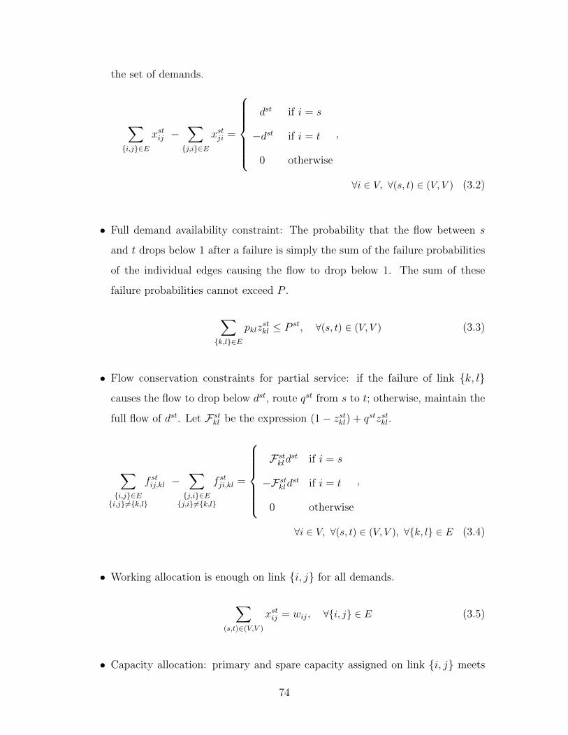
the set of demands.

∑{i,j}∈E

xstij −∑{j,i}∈E

xstji =

dst if i = s

−dst if i = t

0 otherwise

,

∀i ∈ V, ∀(s, t) ∈ (V, V ) (3.2)

• Full demand availability constraint: The probability that the flow between s

and t drops below 1 after a failure is simply the sum of the failure probabilities

of the individual edges causing the flow to drop below 1. The sum of these

failure probabilities cannot exceed P .

∑{k,l}∈E

pklzstkl ≤ P st, ∀(s, t) ∈ (V, V ) (3.3)

• Flow conservation constraints for partial service: if the failure of link {k, l}

causes the flow to drop below dst, route qst from s to t; otherwise, maintain the

full flow of dst. Let F stkl be the expression (1− zstkl) + qstzstkl.

∑{i,j}∈E{i,j}6={k,l}

f stij,kl −∑{j,i}∈E{j,i}6={k,l}

f stji,kl =

F stkldst if i = s

−F stkldst if i = t

0 otherwise

,

∀i ∈ V, ∀(s, t) ∈ (V, V ), ∀{k, l} ∈ E (3.4)

• Working allocation is enough on link {i, j} for all demands.

∑(s,t)∈(V,V )

xstij = wij, ∀{i, j} ∈ E (3.5)

• Capacity allocation: primary and spare capacity assigned on link {i, j} meets

74

2

1

3

45

6

7

8

9

10

11

12

13

14

Figure 3-2: 14 Node NSFNET backbone network

protection requirements after the failure of link {k, l}.

f stij,kl ≤ xstij + ystij,kl,∀{i,j}∈E, ∀{k,l}∈E∀(s,t)∈(V,V ) (3.6)

• Spare allocation is enough on link {i, j} for all demands after failure of edge

{k, l}

∑(s,t)∈(V,V )

ystij,kl ≤ sij,∀{i,j}∈E∀{k,l}∈E (3.7)

For some demand between nodes s and t, a minimum-cost solution will provide

an edge capacity allocation such that the flow drops to a fraction qst of that demand

with at most probability P st.

3.3.2 Comparison to Full Protection

Multiple availability guaranteed protection is compared to the 1 + 1 full protection

scheme via simulation. The performance of the strategies is compared using the

NSFNET topology (Fig. 3-2) with 100 random unit demands. The protection re-

quirement q is set to 12

for all demands. All link costs are set to 1, and the probability

of failure for any link is proportional to its length, which is reasonable since a longer

fiber will have a higher likelihood of being accidently cut. The maximum failure

probability P is varied from 0 to .3 by .05 increments. While the main focus of this

75

150

200

250

300

350

400

450

500

550

0 0.05 0.1 0.15 0.2 0.25 0.3

Cos

t

Max Failure Probability

1+1 MAGP: No Bif MAGP: Bif SP

Figure 3-3: Capacity cost vs. MFP with q = 12

chapter is the case where the primary flow is restricted to a single path, this simu-

lation also considers allowing the primary flow to be bifurcated. Bifurcation reduces

the loss of flow after any edge failure, thereby reducing the total allocation needed to

meet requirements. Relaxing the integer constraint on the primary flow variables in

the MILP corresponds to enabling bifurcation of the primary flow. Routing solutions

for MAGP were determined using CPLEX to solve the MILP. Due to the length of

running time of the MILP, each demand is run individually, which is the case without

protection resource sharing. Protection resource sharing is considered in Section 3.5,

where a one-at-a-time routing scheme is utilized. The shortest pair of disjoint paths

were used for 1 + 1 protection [34].

The average cost to route the demand and protection capacity using the different

routing strategies is plotted in Fig. 3-3 as a function of the maximum failure prob-

ability P . The shortest path routing without protection considerations is used as a

lower bound. The cost of providing incremental protection with parameters q and P

is the difference between the cost of the respective protection strategies and shortest

path routing.

76

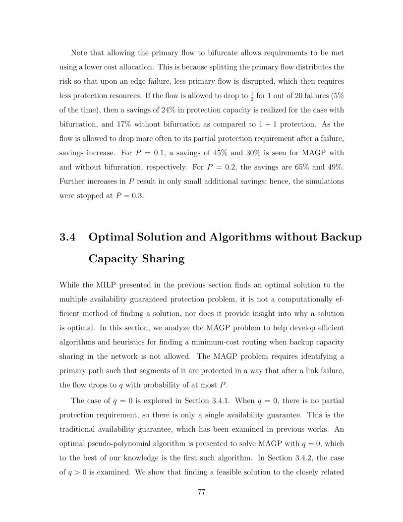
Note that allowing the primary flow to bifurcate allows requirements to be met

using a lower cost allocation. This is because splitting the primary flow distributes the

risk so that upon an edge failure, less primary flow is disrupted, which then requires

less protection resources. If the flow is allowed to drop to 12

for 1 out of 20 failures (5%

of the time), then a savings of 24% in protection capacity is realized for the case with

bifurcation, and 17% without bifurcation as compared to 1 + 1 protection. As the

flow is allowed to drop more often to its partial protection requirement after a failure,

savings increase. For P = 0.1, a savings of 45% and 30% is seen for MAGP with

and without bifurcation, respectively. For P = 0.2, the savings are 65% and 49%.

Further increases in P result in only small additional savings; hence, the simulations

were stopped at P = 0.3.

3.4 Optimal Solution and Algorithms without Backup

Capacity Sharing

While the MILP presented in the previous section finds an optimal solution to the

multiple availability guaranteed protection problem, it is not a computationally ef-

ficient method of finding a solution, nor does it provide insight into why a solution

is optimal. In this section, we analyze the MAGP problem to help develop efficient

algorithms and heuristics for finding a minimum-cost routing when backup capacity

sharing in the network is not allowed. The MAGP problem requires identifying a

primary path such that segments of it are protected in a way that after a link failure,

the flow drops to q with probability of at most P .

The case of q = 0 is explored in Section 3.4.1. When q = 0, there is no partial

protection requirement, so there is only a single availability guarantee. This is the

traditional availability guarantee, which has been examined in previous works. An

optimal pseudo-polynomial algorithm is presented to solve MAGP with q = 0, which

to the best of our knowledge is the first such algorithm. In Section 3.4.2, the case

of q > 0 is examined. We show that finding a feasible solution to the closely related

77

problem of Singly Constrained Shortest Pair of Disjoint Paths is strongly NP-Hard

(there exists no pseudo-polynomial or ε-approximation algorithm), and conjecture

that the MAGP problem with q > 0 is also strongly NP-Hard. Hence, a heuristic for

solving MAGP with q > 0 is developed. Multiple Availability Guaranteed Protection

with the use of backup capacity sharing is examined in Section 3.5.

3.4.1 Availability Guarantees with q = 0

When q = 0, the partial protection requirement is removed and no flow is needed

during the downtime. To solve this problem, a primary path needs to be found such

that segments of it are protected, and after a failure, the flow can drop to 0 with

probability of at most P . First, a restricted version of the problem is considered

where we try to meet availability requirements without the use of spare allocation. It

can be shown that the solution to the restricted problem is the constrained shortest

path (CSP) problem [29]. Next, the problem without restrictions on spare allocation

is studied. We transform this unrestricted problem to an instance of the restricted

one, and use CSP to find an optimal pseudo-polynomial algorithm for MAGP when

q = 0.

Availability Guarantees Without Spare Allocation

First, we consider finding the lowest-cost path between s and t that meets the avail-

ability guarantee without the use of spare allocation. In other words, we want to

find the lowest-cost path such that the sum of all the failure probabilities in that

path are less than P . This problem is recognized to be the constrained shortest path

problem (CSP) [29], which is NP-Hard. A dynamic program exists that finds the

minimum-cost solution to CSP in pseudo-polynomial time [56], with a running time

of O(n2P ), where n is the number of nodes in the network; the P factor is what

makes this running time pseudo-polynomial. CSP assumes all inputs are integer, so

instead of the failure probabilities being between 0 and 1, we multiply P and all pij

values, ∀{i, j} ∈ E, by the smallest factor that makes all the values integer (all inputs

78

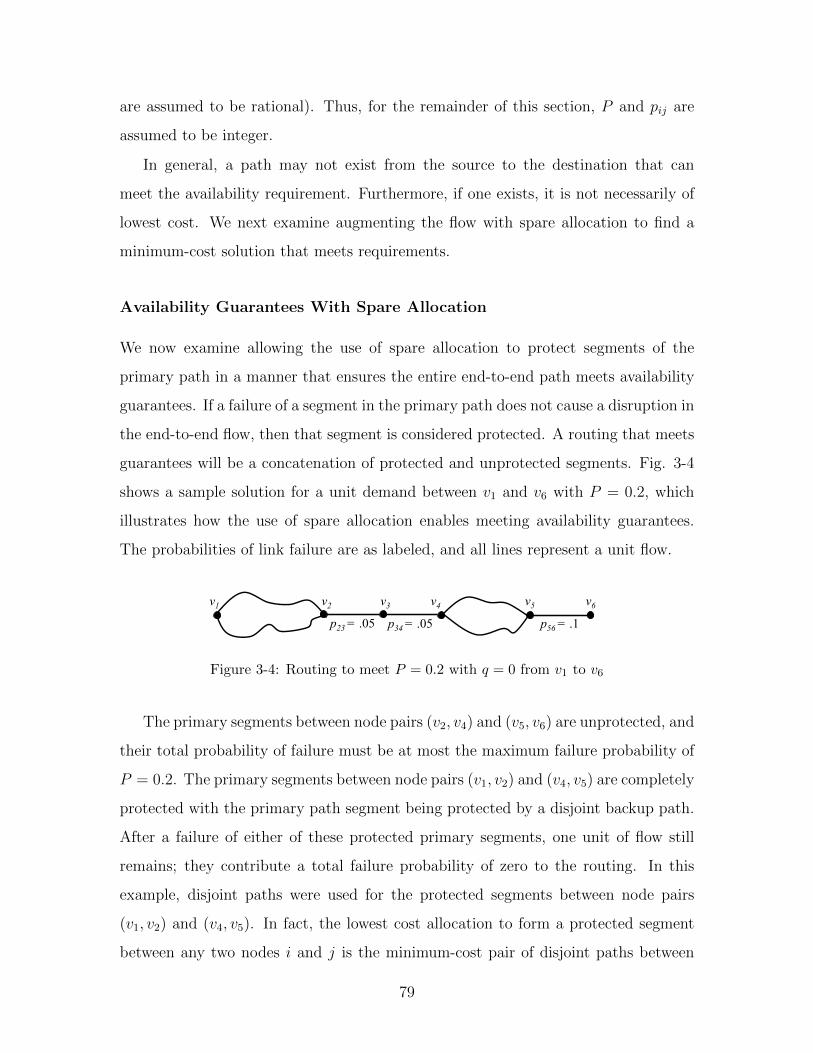
are assumed to be rational). Thus, for the remainder of this section, P and pij are

assumed to be integer.

In general, a path may not exist from the source to the destination that can

meet the availability requirement. Furthermore, if one exists, it is not necessarily of

lowest cost. We next examine augmenting the flow with spare allocation to find a

minimum-cost solution that meets requirements.

Availability Guarantees With Spare Allocation

We now examine allowing the use of spare allocation to protect segments of the

primary path in a manner that ensures the entire end-to-end path meets availability

guarantees. If a failure of a segment in the primary path does not cause a disruption in

the end-to-end flow, then that segment is considered protected. A routing that meets

guarantees will be a concatenation of protected and unprotected segments. Fig. 3-4

shows a sample solution for a unit demand between v1 and v6 with P = 0.2, which

illustrates how the use of spare allocation enables meeting availability guarantees.

The probabilities of link failure are as labeled, and all lines represent a unit flow.

v1 v2 v3 v4 v5 v6

p23 = .05 p34 = .05 p56 = .1

Figure 3-4: Routing to meet P = 0.2 with q = 0 from v1 to v6

The primary segments between node pairs (v2, v4) and (v5, v6) are unprotected, and

their total probability of failure must be at most the maximum failure probability of

P = 0.2. The primary segments between node pairs (v1, v2) and (v4, v5) are completely

protected with the primary path segment being protected by a disjoint backup path.

After a failure of either of these protected primary segments, one unit of flow still

remains; they contribute a total failure probability of zero to the routing. In this

example, disjoint paths were used for the protected segments between node pairs

(v1, v2) and (v4, v5). In fact, the lowest cost allocation to form a protected segment

between any two nodes i and j is the minimum-cost pair of disjoint paths between

79

the two, as demonstrated in Lemma 3.1.

Lemma 3.1. The minimum-cost protected segment between nodes i and j is the

minimum-cost pair of disjoint paths.

Proof. For a segment between i and j to be protected, 1 unit of flow must remain

between the source and destination after any single edge failure in the primary path.

No backup edge will have an allocation greater than 1 because the primary flow will

have 1 unit, and exactly 1 unit will need to be restored after any primary failure. An

equivalent problem is to find the lowest-cost routing for 2 units of flow between i and

j in a network where every edge has a maximum capacity of 1. After any single edge

failure, at least 1 unit of flow will remain. This is a minimum-cost flow problem [29],

whose solution has integer flows when given integer inputs. Since every edge has a

capacity of 1, there will be two distinct edge-disjoint flows of 1 unit each. Clearly,

the lowest-cost solution has these flows routed on the minimum-cost pair of disjoint

paths.

Using Lemma 3.1, every possible protected segment between any two nodes can

be transformed to a single edge with a failure probability of 0 and a cost equivalent to

the minimum-cost pair of disjoint paths between the nodes. We denote the cost and

probability of the minimum-cost pair of disjoint paths between nodes i and j as cij

and pij = 0, respectively. Now, any protected segment between some node pair (i, j)

can be represented as a single edge between i and j in the network. This edge contains

the primary and spare allocation that would be used if a protected segment between

i and j was needed. Adding an edge for every possible protected segment transforms

the problem back to the restricted version where no spare allocation was allowed.

This problem can now be solved using the constrained shortest path algorithm.

Our proposed algorithm is as follows. We take the graph G, where every edge

has a cost and a failure probability associated with it, and augment the graph with

an edge between every pair of nodes (i, j) such that the cost of that edge is the

minimum-cost pair of disjoint paths between i and j, and the probability of failure

for that edge is zero. Thus the new augmented graph has two kinds of edges between

80

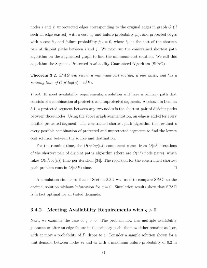
nodes i and j: unprotected edges corresponding to the original edges in graph G (if

such an edge existed) with a cost cij and failure probability pij, and protected edges

with a cost cij and failure probability pij = 0, where cij is the cost of the shortest

pair of disjoint paths between i and j. We next run the constrained shortest path

algorithm on the augmented graph to find the minimum-cost solution. We call this

algorithm the Segment Protected Availability Guaranteed Algorithm (SPAG).

Theorem 3.2. SPAG will return a minimum-cost routing, if one exists, and has a

running time of O(n4log(n) + n2P ).

Proof. To meet availability requirements, a solution will have a primary path that

consists of a combination of protected and unprotected segments. As shown in Lemma

3.1, a protected segment between any two nodes is the shortest pair of disjoint paths

between those nodes. Using the above graph augmentation, an edge is added for every

feasible protected segment. The constrained shortest path algorithm then evaluates

every possible combination of protected and unprotected segments to find the lowest

cost solution between the source and destination.

For the running time, the O(n4log(n)) component comes from O(n2) iterations

of the shortest pair of disjoint paths algorithm (there are O(n2) node pairs), which

takes O(n2log(n)) time per iteration [34]. The recursion for the constrained shortest

path problem runs in O(n2P ) time.

A simulation similar to that of Section 3.3.2 was used to compare SPAG to the

optimal solution without bifurcation for q = 0. Simulation results show that SPAG

is in fact optimal for all tested demands.

3.4.2 Meeting Availability Requirements with q > 0

Next, we examine the case of q > 0. The problem now has multiple availability

guarantees: after an edge failure in the primary path, the flow either remains at 1 or,

with at most a probability of P , drops to q. Consider a sample solution shown for a

unit demand between nodes v1 and v6 with a maximum failure probability of 0.2 in

81

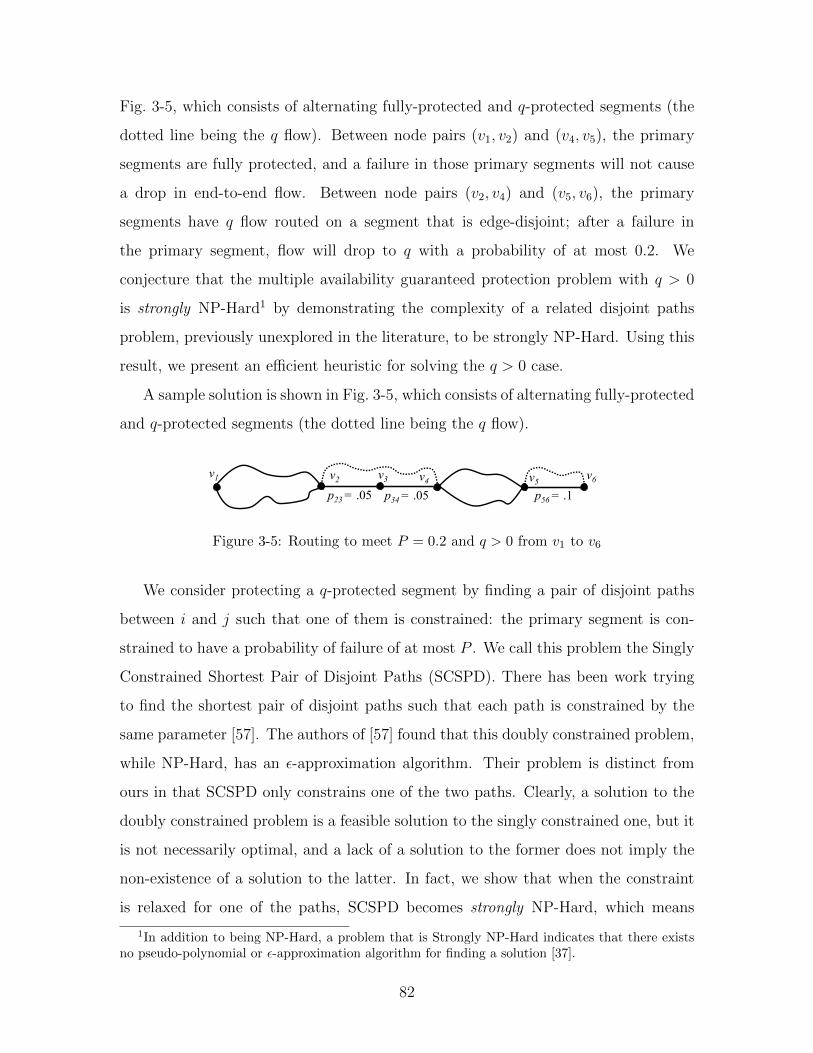
Fig. 3-5, which consists of alternating fully-protected and q-protected segments (the

dotted line being the q flow). Between node pairs (v1, v2) and (v4, v5), the primary

segments are fully protected, and a failure in those primary segments will not cause

a drop in end-to-end flow. Between node pairs (v2, v4) and (v5, v6), the primary

segments have q flow routed on a segment that is edge-disjoint; after a failure in

the primary segment, flow will drop to q with a probability of at most 0.2. We

conjecture that the multiple availability guaranteed protection problem with q > 0

is strongly NP-Hard1 by demonstrating the complexity of a related disjoint paths

problem, previously unexplored in the literature, to be strongly NP-Hard. Using this

result, we present an efficient heuristic for solving the q > 0 case.

A sample solution is shown in Fig. 3-5, which consists of alternating fully-protected

and q-protected segments (the dotted line being the q flow).

v1 v2 v3 v4 v5 v6 p23 = .05 p34 = .05 p56 = .1

Figure 3-5: Routing to meet P = 0.2 and q > 0 from v1 to v6

We consider protecting a q-protected segment by finding a pair of disjoint paths

between i and j such that one of them is constrained: the primary segment is con-

strained to have a probability of failure of at most P . We call this problem the Singly

Constrained Shortest Pair of Disjoint Paths (SCSPD). There has been work trying

to find the shortest pair of disjoint paths such that each path is constrained by the

same parameter [57]. The authors of [57] found that this doubly constrained problem,

while NP-Hard, has an ε-approximation algorithm. Their problem is distinct from

ours in that SCSPD only constrains one of the two paths. Clearly, a solution to the

doubly constrained problem is a feasible solution to the singly constrained one, but it

is not necessarily optimal, and a lack of a solution to the former does not imply the

non-existence of a solution to the latter. In fact, we show that when the constraint

is relaxed for one of the paths, SCSPD becomes strongly NP-Hard, which means

1In addition to being NP-Hard, a problem that is Strongly NP-Hard indicates that there existsno pseudo-polynomial or ε-approximation algorithm for finding a solution [37].

82

300

350

400

450

500

550

600

0 0.025 0.05 0.075 0.1 0.125 0.15 0.175 0.2

Cos

t


SPMAG

Opt

Figure 3-6: SPMAG capacity cost vs. MFP with q = 12

that a solution cannot be ε-approximated, nor can there be any pseudo-polynomial

algorithm for optimality [37].

Theorem 3.3. The Singly Constrained Shortest Pair of Disjoint Paths problem is

strongly NP-Hard.

Proof. To demonstrate strong NP-Hardness of SCSPD, a reduction from the 3SAT

problem [1] is performed. See Chapter Appendix Section 3.7.2 for the complete proof.

Since SCSPD is strongly NP-Hard, the dynamic programming approach used to

solve for q = 0 does not work when q > 0. We conjecture that the multiple availability

guaranteed protection when q > 0 is in fact also strongly NP-Hard, thereby necessi-

tating a heuristic approach to solve the problem. Our proposed heuristic augments

the q = 0 algorithm: after an optimal solution for q = 0 is found, find the shortest

disjoint path for the unprotected segments and allocate a flow of q to them. We call

this algorithm the Segment Protected Multiple Availability Guaranteed Algorithm

(SPMAG).

83

A simulation similar to that of Section 3.3.2 was run comparing SPMAG and the

optimal solution to MAGP without flow bifurcation; the results are plotted in Figure

3-6. On average, SPMAG performs within 6% of the optimal solution to the multiple

availability guaranteed protection problem.

3.5 Algorithm with Backup Capacity Sharing

In the previous section, efficient algorithms were presented without the use of backup

capacity sharing, including an optimal algorithm for the case of q = 0, which corre-

sponds to the standard availability constraint. These results are useful for a basic

understanding of the Multiple Availability Guaranteed Protection problem (MAGP),

and for networks that do not allow protection sharing. But many times, networks do

utilize backup sharing, and significant savings can often be achieved. In this section,

a time-efficient algorithm for MAGP using backup capacity sharing is presented.


then under a single-link failure model, at most one can be disrupted at any given

point in time. Since at most one demand will need to be restored after a failure, two

failure-disjoint flows can share backup capacity.

Determining how much backup capacity can be shared for 1+1 guaranteed pro-

tection was examined in [18] and [19]. These papers used conflict sets to determine

potential backup sharing on an edge by keeping track of how much backup capacity

was allocated on one edge to protect against the failure of another. If more backup

capacity is already allocated on some edge than is needed to protect for the failure

of another edge, then that edge’s backup capacity can be shared. This model can

be extended to the partial protection framework by guaranteeing that any particular

demand has its partial flow requirement met after a failure. An example without

probabilistic availability guarantees is given in Fig. 3-7. Define the variable hklij to

be the number of units of capacity used on edge {i, j} to protect against the failure

of edge {k, l}. The maximum number of units allocated on edge {i, j} to protect

against any edge failure is the total spare allocation needed on {i, j}. In Fig. 3-7,

84

two demands with q1 = 1 and q2 = 12

are routed. Both demands use edge {i, j} for

protection with 1 unit being needed after the failure of {k, l} and 12

unit being needed

after the failure of {m,n}. In this example we have hklij = 1 and hmnij = 12.

Figure 3-7: Example of a conflict set with partial protection

Now, consider a new demand with q3 = 12. If this demand were to have its primary

flow routed on edge {k, l} and use {i, j} for protection, hklij will increase by 12

unit.

Since the amount of spare allocation on an edge is the maximum capacity needed to

protect against any edge failure, the total allocation will increase by 12. Alternatively,

if the demand were to use {m,n} instead of {k, l}, hmnij will increase by 12, and the

maximum number of units needed to protect against any edge failure will still only

be 1. No additional resources are required for protection on {i, j} under this routing

scenario. For the exact implementation of conflict sets for protection resource sharing,

see [18, 19].

We now consider meeting probabilistic availability guarantees. Given some pri-

mary path between s and t, certain segments will be fully-protected, and others will

be partially protected with a flow of q. For each edge in the primary path, the cost

of using 1 or q units on edge {i, j} for backup is calculated using conflict sets. For a

primary path with a set of edges S, let B(S, 1) be the cost of backup edges for fully

protecting any edge, and B(S, q) be the cost of backup edges that partially protect

an edge with a flow of q.

Next, we calculate the cost of protecting each possible segment of a given primary

path with either full or partial protection; if there are v nodes in the primary path,

then there are v(v−1)2

segments contained within that path. We construct a new

graph GstS with two edges between every pair of nodes in the primary path; these two

edges correspond to fully or partially protecting the primary segment between nodes

85

i and j. For every primary segment in the primary path, we find two paths that are

disjoint to that segment: one that fully protects that segment, and one that partially

protects it. For full protection, the edge between nodes i and j in GstS is the shortest

disjoint path to primary segment (i, j) using the set of edge costs B(S, 1); for partial

protection, the edge between i and j in GstS is the shortest disjoint path to primary

segment (i, j) using B(S, q). The cost of the edge in GstS to fully protect primary

segment (i, j) is c1ij, and has failure probability p1ij = 0. The cost of the edge in GstS

to partially protect primary segment (i, j) is cqij, and has failure probability pqij equal

to the failure probability of the primary path segment between nodes i and j. Once

GstS is fully constructed, we find the constrained shortest path in Gst

S from s to t with

a maximum failure probability of P st. This path will be the backup, which meets

all partial protection and availability requirements when combined with the initial

primary path.

Since jointly optimizing the primary and protection path with backup sharing is

NP-Hard [18], we choose a simple strategy of using the shortest path for the primary.

This is in contrast to [18, 19] that offer a heuristic approach to jointly optimize the

primary and protection path for each incoming demand. Our simulations (presented

at the end of this section) show that using the shortest path for the primary route

actually performs better than jointly optimizing the primary and backup paths for

each incoming demand.

The algorithm for MAGP to route a demand using backup capacity sharing is

as follows. For an arriving demand between s and t, find the shortest path between

those two nodes; Sst will be the set of edges in that shortest path. We then construct

the graph GstS using the backup capacity sharing procedure discussed above, and then

we find the lowest-cost shared backup to meet protection and availability require-

ments. This algorithm is called Dynamic Multiple Availability Guaranteed Segment

Protection (DMAGSP).

An example is shown in Fig. 3-8. A unit demand needs to be routed between v1

and v4, with a maximum failure probability of P = 0.2. For this example, the shortest

path between v1 and v4 has already been found, v1− v2− v3− v4. This shortest path

86

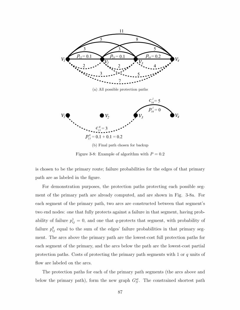
(a) All possible protection paths

(b) Final path chosen for backup

Figure 3-8: Example of algorithm with P = 0.2

is chosen to be the primary route; failure probabilities for the edges of that primary

path are as labeled in the figure.

For demonstration purposes, the protection paths protecting each possible seg-

ment of the primary path are already computed, and are shown in Fig. 3-8a. For

each segment of the primary path, two arcs are constructed between that segment’s

two end nodes: one that fully protects against a failure in that segment, having prob-

ability of failure p1ij = 0, and one that q-protects that segment, with probability of

failure pqij equal to the sum of the edges’ failure probabilities in that primary seg-

ment. The arcs above the primary path are the lowest-cost full protection paths for

each segment of the primary, and the arcs below the path are the lowest-cost partial

protection paths. Costs of protecting the primary path segments with 1 or q units of

flow are labeled on the arcs.

The protection paths for each of the primary path segments (the arcs above and

below the primary path), form the new graph GstS . The constrained shortest path

87

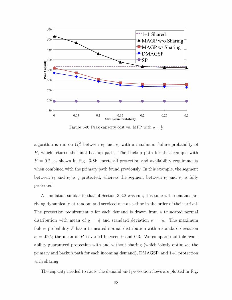
150

200

250

300

350

400

450

500

550

0 0.05 0.1 0.15 0.2 0.25 0.3

Peak

Cap

acity


1+1 Shared MAGP w/o Sharing MAGP w/ Sharing DMAGSP SP

Figure 3-9: Peak capacity cost vs. MFP with q = 12

algorithm is run on GstS between v1 and v4 with a maximum failure probability of

P , which returns the final backup path. The backup path for this example with

P = 0.2, as shown in Fig. 3-8b, meets all protection and availability requirements

when combined with the primary path found previously. In this example, the segment

between v1 and v3 is q protected, whereas the segment between v3 and v4 is fully

protected.

A simulation similar to that of Section 3.3.2 was run, this time with demands ar-

riving dynamically at random and serviced one-at-a-time in the order of their arrival.

The protection requirement q for each demand is drawn from a truncated normal

distribution with mean of q = 12

and standard deviation σ = 12. The maximum

failure probability P has a truncated normal distribution with a standard deviation

σ = .025; the mean of P is varied between 0 and 0.3. We compare multiple avail-

ability guaranteed protection with and without sharing (which jointly optimizes the

primary and backup path for each incoming demand), DMAGSP, and 1+1 protection

with sharing.

The capacity needed to route the demand and protection flows are plotted in Fig.

88

3-9 as a function of the expected value of P . Again, the shortest path routing without

protection considerations is used as a lower bound for the capacity allocation. MAGP

with backup sharing, which jointly optimizes the primary and backup paths for each

incoming demand, achieves an average reduction in excess resources of 42% over 1+1

protection with sharing, and a reduction of 51% over MAGP without sharing.

A notable result is that Dynamic Multiple Availability Guaranteed Segment Pro-

tection (DMAGSP) in fact performs better than the greedy optimal solution with

dynamic arrivals. This can be explained by observing that the algorithm takes the

simple strategy of the shortest path as the primary for each connection, as opposed to

jointly optimizing the primary and backup routes, which may take a longer primary

path to take advantage of backup sharing. This longer path makes it potentially more

difficult for future demands to find disjoint primary routes, lowering their ability to

share protection resources. While other works have focused on finding heuristics to

jointly optimize the primary and backup paths for each incoming demand, it appears

a better approach is to simply take the shortest path for the primary route.

3.6 Conclusion

In this chapter, a novel network protection scheme with multiple availability guaran-

tees was introduced. In particular, the multiple availability guarantees will maintain

the full demand for at least a guaranteed fraction of time and guarantee a partial flow

during the downtime. If the demand is allowed to drop to 50% of its flow for only 1

out of every 20 failures, a 24% reduction in excess resources can be realized over the

traditional 1 + 1 full protection scheme. For the q = 0, which corresponds to the pre-

viously studied scenario where full availability is guaranteed for a fraction of time, we

developed an optimal pseudo-polynomial algorithm. For the case of q > 0, we devel-

oped a time-efficient heuristic (Segment Protected Multiple Availability Guaranteed

Protection) that performs within 6% of the optimal solution to the multiple avail-

ability guaranteed protection problem. We then extended the Multiple Availability

Guaranteed Problem (MAGP) to the case where backup capacity sharing is utilized

89

to lower the total amount of resources needed to meet protection and availability

requirements. An algorithm for MAGP with protection sharing was developed for

dynamic arrivals, which in fact performs better than jointly optimizing the primary

and backup paths for each incoming demand.


3.7.1 Proof of NP-Hardness for Multiple Availability Guar-

anteed Protection

To demonstrate NP-Hardness of MAGP, the 1-0 knapsack problem [37] will be reduced

to MAGP. The knapsack problem finds the maximum value subset of k items, with

the ith item having cost ci and weight pi, such that the maximum weight P of the

knapsack is not exceeded.

s t c1

c1

c2

c2

ck

ck p1

p1

p2

p2

pk

pk

Figure 3-10: Sample network for MAGP NP-Hardness proof

Consider the network shown in Fig. 3-10 with link costs and probabilities denoted

by ci and pi, respectively. We wish to find a minimum-cost routing for a unit demand

from s to t with a maximum failure probability P and partial protection requirement

q = 0. After any link failure, the network will either maintain its full flow of 1 unit,

or have no flow with a probability of at most P . There are k distinct link groups,

where each of the two links in any group have the same probability of failure and

cost. Primary flow has to be allocated onto at least one of these links, otherwise

the primary demand cannot be met. If the network maintains full connectivity after

a primary failure in the kth link group, then each link in that group will have an

allocation of 1 unit. If there is no flow after a link failure, then only one link has an

allocation of 1, and the other 0. So, every link group has at least one link with a flow

90

of 1, which is a fixed cost regardless of protection allocation.

To find the lowest cost protection allocation to meet availability guarantees, we

need to find the lowest cost combination of the remaining links after the primary

flow is allocated such that the sum of the failure probabilities for the links that

have no allocation are less than P . Our objective is min∑k

i=1 ci(1 − zi), subject

to the constraint of∑k

i=1 pizi ≤ P , with zi ∈ {0, 1} ∀i ∈ 1, ..., k. The objective

can be rewritten to maximize the cost of the links that do not have allocation:

min∑k

i=1 ci(1 − zi) = max∑k

i=1 cizi. We now recognize this to be the NP-Hard

1-0 knapsack problem with a maximum weight of P , and cost and weight of the ith

item being the cost and probability, respectively, of each pair of links in the ith link

group. If there existed a polynomial time solution to MAGP, then there would exist

one for the 1-0 knapsack problem. Therefore, MAGP is at least as hard as the 1-0

knapsack problem. In addition, we note that our problem is clearly in NP.

3.7.2 Proof of Strong NP-Hardness for Singly Constrained

Shortest Pair of Disjoint Paths

To prove that SCSPDP is strongly NP-Hard, we borrow a reduction that demonstrates

the NP-Hardness of a different, but similar, problem [1] and adapt it to the SCSPD

problem. The authors of [1] attempt to find the “min-min” disjoint pair of paths,

which is defined as the minimum-cost pair of disjoint paths that contains, over all

sets of possible disjoint paths, the minimum-cost shorter path.

s t x1 x2 x3 x4

y1 z1 y2 z2 y3 z3 y4 z4

Figure 3-11: Sample network to solve an instance of 3SAT from [1]

91

To demonstrate this problem is NP-Hard, they construct a mapping of the 3SAT

problem to a graph where a solution to their problem will simultaneously solve the

3SAT problem. A solution to 3SAT determines if there exists a 1/0 assignment to

the variables that will make a specific boolean expression true [37]. The graph in

Fig. 3-11 is a sample network corresponding to the instance of the 3SAT problem of

(x1 ∨ x2 ∨ x3)∧ (x1 ∨ x3 ∨ x4)∧ (x2 ∨ x3 ∨ x4)∧ (x2 ∨ x3 ∨ x4) [1]. Without going into

the specifics of the reduction (see [1] for details), a generalized version of their result

is: if two disjoint paths can be found between s and t such that one of them uses only

the dotted lines, then that solution is also a solution to the 3SAT problem (see [1]

for the proof). To demonstrate strong NP-Hardness, one needs to show the problem

remains NP-Hard after the value of all inputs to the system have been bounded by

some polynomial [37].

We will first show the problem to be NP-Hard by assigining costs and probabil-

ities to the edges of the above network such that solving SCSPD will also solve the

3SAT problem. Then, we will demonstrate that SCSPD is in fact strongly NP-Hard.

Assume there exists D dotted edges and L solid edges in the 3SAT reduced graph.

Since we can assign parameters of our choosing to the edges, assign a cost of 0 for

the dotted edges and a cost of 1 to the solid edges. We choose the failure probability

of each dotted edge to be αD

and the probability of each solid edge to be 1−αL

, such

that α ≤ 1−αL→ α ≤ 1

1+L. Additionally, choose a maximum probability of failure P

such that α ≤ P < 1−αL

. Since using any solid edge will make that path violate the

maximum failure probability P , the only feasible solution to SCSPD on this network

is for the constrained path to use only dotted edges. But if such a solution could

be found, it would solve the 3SAT problem, which is NP-Hard. The problem in

fact remains NP-hard when all input values are polynomial bounded: L and D are

polynomial bounded by the number of inputs from the 3SAT problem, and α can be

chosen to be polynomial bounded. If all input parameters to a problem are bounded

by some polynomial, and the problem remains NP-Hard, then the problem is strongly

NP-Hard [37]. Finding any feasible solution to SCSPD on this bounded graph will

still solve the 3SAT problem. Therefore, SCSPD is strongly NP-Hard.

92

Chapter 4

Protection with Guaranteed

Recovery Times using Recovery

Domains

In the previous Chapters 2 and 3 of this thesis, we considered offering alternatives to

guaranteed full protection that allowed for a demand to be at a guaranteed level of

partial service either after any service disruption, or only with a certain probability

after a service disruption. Instead of the service guarantee of partial service, in this

chapter, we consider the service guarantee of maximum recovery time after a failure.

4.1 Introduction

As the importance of time-sensitive internet traffic continues to rise, there is an in-

creasing need to offer network protection that provides guarantees on the amount of

time flow can be disrupted after a failure. Examples of time-sensitive traffic include

voice-over-IP and video streaming, which would be rendered unusable with high la-

tency delays. Many networks employ protection techniques that offer no recovery

time guarantees whatsoever. Alternatively, networks typically provide local recovery

schemes, which reroute a connection at the point of failure; such schemes typically

over-provision resources to meet time recovery constraints. In this chapter, we a

93

present novel solution that provides guarantees on the maximum amount of time

that flow can be disrupted after a failure, which is both flexible and efficient. We

refer to these time guarantees as the recovery time of the network.

Protection in the internet has traditionally been accomplished using a real-time

rerouting approach: after a link failure occurs, the network is updated with the new

set of shortest paths between node pairs, and then a new path is selected. This is both

slow (sometimes on the order of minutes) [11], and does not necessarily guarantee that

bandwidth will be available for the new path [12, 13]. Despite its slow recovery time,

this approach is still commonly used in backbone networks [8]. In the past decade,

Multi-Protocol Label Switching (MPLS) has been developed to support constraint

based routing, which allows connections to be made with guarantees on parameters

such as bandwidth, latency, and recovery time [59]. Because of its flexibility and traffic

engineering capabilities, MPLS has become the leading packet transport network

technology in backbone networks [60]. To handle these fast recovery times, the Fast

ReRoute (FRR) framework was developed to be used within MPLS [38]. FRR is a

local recovery scheme where traffic is routed away from the node directly preceding

a fault, which is known as the point of local repair (PLR), and reconnects with the

original path at the merge point (MP). Various implementations of local recovery

have been previously examined [61–65].

More recently, the new IETF standard for the MPLS Transport Profile (MPLS-

TP) Protection Framework calls for the creation of “recovery domains” [39]. Recovery

domains are defined to be non-overlapping path segments, such that after a failure

within a segment, flow is restored using a back-up path between the end-points of

that segment. Moreover, recovery domains connect to one another via their respective

“reference” end-points, forming an end-to-end protected flow. An example is shown

in Fig. 4-1: after the failure of an edge in the primary path located within Recovery

Domain 2, the recovery domain’s upstream end-point redirects flow onto the backup

path, which then reconnects at that recovery domain’s downstream end-point, by-

passing the failure. The recovery domain model can be used to provide recovery time

guarantees.

94

Recovery Domain 1

Recovery Domain 2

Recovery Domain 3

Figure 4-1: End-to-end routing using recovery domains

In local recovery, since each possible failure has its own dedicated protection path,

resources are often over-provisioned beyond what is needed to meet recovery time

guarantees. Consider the example shown Fig. 4-2; the propagation delay for each

link is 10 ms, and switching delays are assumed to be negligible. A flow needs to

be found from v1 to v5 such that the maximum time that the flow can be disripted

after a failure is 50 ms, which is the typical recovery time for MPLS networks [11]. A

primary path is already allocated on the solid lines from v1 to v5. A solution to FRR

local recovery is to use all of the links above the primary path: after a link failure

in the primary path, a fault notification is sent to the immediate upstream node of

that failed link, and the flow is then switched to an alternate path from that node

back towards the destination. This protection scheme requires 7 edges to be used for

backup.

v1 v2 v3 v4 v5

Figure 4-2: Time guaranteed recovery examples

Now consider an alternative protection routing using the recovery domain model.

95

Two recovery domains are created by using the links below the primary path as the

backup paths: one recovery domain between nodes v1 and v3, and one between v3

and v5. If link {v2, v3} fails, it would take up to 20 ms for the fault notification to

propagate to v1, and then 20 ms for the data that was switched to the protection

route to reconnect with the primary path at node v3. The other recovery domain will

have a similar recovery time after a failure. In this example, only 4 additional links

are needed to meet protection guarantees when using recovery domains, as opposed

to the 7 needed for FRR.

Previous work has examined providing differentiated reliability for connections,

including maximum recovery times. These papers build off of the segment protection

framework [66], where segments of a primary path are individually protected, but

can overlap by any number of edges. Various heuristics have been considered for

segment protection with recovery time considerations [67–69], and an integer linear

program (ILP) was presented in [70]. In contrast, recovery domains simplify recovery

by separating a flow into disjoint protection regions, where each region guarantees

protection for the flow between its end-points. This flow partitioning approach allows

the network to be decomposed into a set of individual recovery domains, simplifying

capacity allocation and flow control. To the best of our knowledge, the guaranteed

recovery time problem using recovery domains has not yet been examined.

Our novel formulation to provide Guaranteed Recovery Times using Recovery Do-

mains (GRT-RD) allows for a general and efficient set of solutions and algorithms.

We first present a model of the problem in Section 4.2. We then show in Section

4.3 that the recovery domain problem is NP-Hard, and formulate the optimal solu-

tion using an MILP. In Section 4.4, we decompose the end-to-end recovery domain

problem into more tractable subproblems, which allows us to more easily construct

a solution for the end-to-end problem. This allows for the development of flexible

and efficient solutions, including an optimal algorithm using Lagrangian relaxation,

which simulations show to converge rapidly to an optimal solution. In Section 4.5,

an algorithm is developed for the case when backup sharing is allowed.

96

4.2 Model and Problem Description

In this chapter, solutions to the problem of Guaranteed Recovery Time using Recov-

ery Domains (GRT-RD) are developed and analyzed. The objective is to provide a

primary and protection path for each demand, such that the amount of time flow is

disrupted after a failure is guaranteed to be no greater than some maximum value. In

order to meet these recovery time guarantees, we separate an end-to-end flow into “re-

covery domains”, where within each recovery domain, the maximum time to recover

from a failure cannot exceed a given value. We borrow the definition of recovery

domains from [39]: “A recovery domain is defined between two recovery reference

end-points which are located at the edges of the recovery domain... To guarantee

protection in all situations, a dedicated recovery entity should be pre-provisioned us-

ing disjoint resources in the recovery domain, in order to protect against a failure of

a working entity.”

Adding the constraint for time guaranteed recovery, we implement GRT-RD as

follows: an end-to-end recovery domain routing is a set of recovery domains connecting

at their respective end-points such that they form a path from the source to the

destination, and that the maximum amount of time a flow can be disrupted after any

single-link failure is guaranteed. An example was shown in Fig. 4-1. We implement

guaranteed protection within a recovery domain using the 1+1 protection scheme,

which provides an edge-disjoint backup path for each primary path, and guarantees

the full flow to be available at all times after any single-link failure [5, 18].

The following network model is used for the remainder of the chapter. A graph G

has a set of vertices V and edges E. We assume a single-link failure model. An end-

to-end recovery domain routing will comprise of a set of recovery domains, connected

via their reference end-nodes, which form an end-to-end flow from a source to its

destination. The maximum recovery time T will be the maximum time data flow can

be interrupted: after a link failure of the primary path in some recovery domain, the

length of time for the primary flow to be rerouted from the upstream reference end-

node to the downstream reference end-node cannot exceed the maximum recovery

97

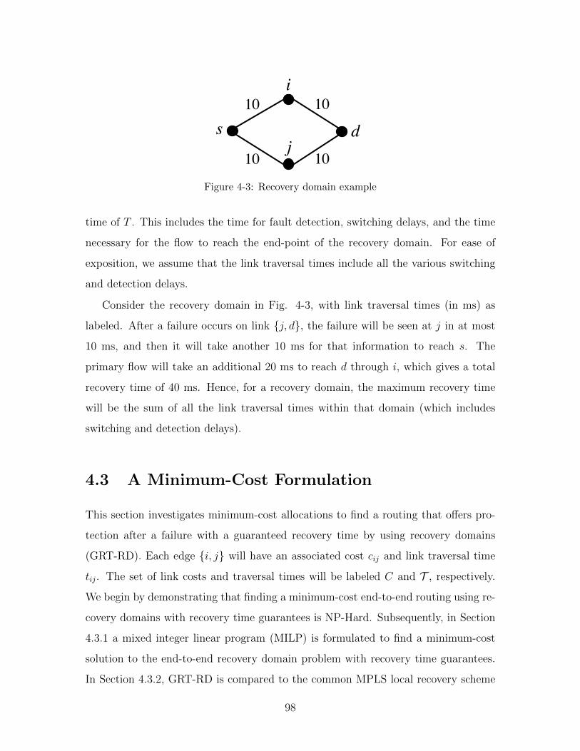
s

i

d j

10 10

10 10

Figure 4-3: Recovery domain example

time of T . This includes the time for fault detection, switching delays, and the time

necessary for the flow to reach the end-point of the recovery domain. For ease of

exposition, we assume that the link traversal times include all the various switching

and detection delays.

Consider the recovery domain in Fig. 4-3, with link traversal times (in ms) as

labeled. After a failure occurs on link {j, d}, the failure will be seen at j in at most

10 ms, and then it will take another 10 ms for that information to reach s. The

primary flow will take an additional 20 ms to reach d through i, which gives a total

recovery time of 40 ms. Hence, for a recovery domain, the maximum recovery time

will be the sum of all the link traversal times within that domain (which includes

switching and detection delays).

4.3 A Minimum-Cost Formulation

This section investigates minimum-cost allocations to find a routing that offers pro-

tection after a failure with a guaranteed recovery time by using recovery domains

(GRT-RD). Each edge {i, j} will have an associated cost cij and link traversal time

tij. The set of link costs and traversal times will be labeled C and T , respectively.

We begin by demonstrating that finding a minimum-cost end-to-end routing using re-

covery domains with recovery time guarantees is NP-Hard. Subsequently, in Section

4.3.1 a mixed integer linear program (MILP) is formulated to find a minimum-cost

solution to the end-to-end recovery domain problem with recovery time guarantees.

In Section 4.3.2, GRT-RD is compared to the common MPLS local recovery scheme

98

of Fast ReRoute (FRR).

We first show that solving for an individual recovery domain with a guaranteed

recovery time is NP-hard. Afterwards, the end-to-end problem is shown to be NP-

hard as well.

Theorem 4.1. Finding the minimum-cost allocation for a pair of disjoint paths be-

tween nodes k and l such that the sum of the link traversals across the two paths does

not exceed some maximum time T is NP-hard.

Proof. We reduce the NP-hard Constrained Shortest Path (CSP) problem [29] to

ours. In CSP, each edge {i, j} has two associated values: cij and tij. In our case

cij is the cost of the edge, and tij is the link traversal time. If xij is a binary flow

variable for edge {i, j}, then the objective is to find a path from k to l that minimizes∑{i,j}∈E cijxij, such that

∑{i,j}∈E tijxij ≤ T . To find a minimum-cost solution to

CSP by solving GRT-RD with a maximum recovery time of T , add a path between

k and l with a total traversal time of zero and a cost of −(∑{i,j}∈E |cij| + 1). A

minimum-cost solution to GRT-RD, if it exists, will always use this path as one of

the two disjoint paths, and the other path will be the solution for CSP from k to l

with a maximum traversal time of T . In addition, we note that our problem is clearly

in NP.

Next, we show that finding an end-to-end routing using recovery domains that

guarantees the maximum length of flow interruption is NP-hard by using a similar

proof to Theorem 4.1. An end-to-end recovery domain routing can have a series of

recovery domains in sequence, each guaranteeing recovery time for its respective flow.

Theorem 4.2. Finding the minimum-cost allocation for a protection routing between

nodes s and d that guarantees a maximum recovery time of T by using end-to-end

recovery domains is NP-hard.

Proof. We add a path between s and d with a total traversal time of zero and a cost of

−(∑{i,j}∈E |cij|+1). Any minimum-cost solution to the end-to-end GRT-RD will use

this negative cost path if a constrained shortest path (CSP) from s to d exists with

99

maximum traversal time of T . Hence, if the minimum-cost solution to the end-to-end

problem uses this negative cost path, then the CSP problem has also been solved.

If the negative cost path is not used, there exists no solution to CSP on the given

network. In addition, we note our problem is clearly in NP.

4.3.1 MILP to find a Minimum-Cost Solution

Since finding a minimum-cost solution for the guaranteed recovery time problem using

recovery domains is NP-hard, in this section a mixed integer linear program (MILP)

is developed to solve for the minimum-cost solution. Two versions are developed: one

for when backup capacity sharing is not allowed, and one when it is. Backup capacity

can be shared between two demands if their primary path edges are disjoint under a

single-link failure model. If a failure occurs, and the two primary paths are disjoint,

then at most one demand can fail. Hence, at most one demand will need backup

protection at a time, and the two demands can share backup protection resources.

Due to space constraints, only the MILP for the non-sharing case is presented here.

The formulation for when protection sharing is allowed can be found in the Chapter

Appendix Section 4.7.1.

Solving for an end-to-end protection routing between nodes s and d using recovery

domains relies on the following observations: each pair of nodes in the network is a

potential recovery domain, and an end-to-end recovery domain routing will be some

subset of these recovery domains. Additionally, in an end-to-end recovery domain

routing, recovery domains connect only via their reference end-points, and each re-

covery domain consists of a pair of edge-disjoint paths. Hence, an end-to-end recovery

domain routing is, in fact, a pair of edge-disjoint paths between s and d (potentially

connected at certain nodes). Using these observations, the MILP is structured as

such: a pair of disjoint paths is found from s to d, where each edge from that pair

of disjoint paths is associated with exactly one recovery domain. Additionally, any

active recovery domain (i.e., part of the solution) must itself consist of a pair of dis-

joint paths between the end-nodes of that recovery domain, and the sum of the link

traversal times of that recovery domain may not exceed the maximum recovery time.

100

Without loss of generality, a unit demand between s and d is assumed.


• G = (V,E) is the graph with a set of vertices and edges

• s is the source and d is the destination


• tij is the traversal time for link {i, j}

• T is the maximum recovery time

The following variables will be solved for:

• xij is 1 if flow is assigned on link {i, j}, and 0 otherwise

• Rkl is 1 if the recovery domain with end nodes k and l is active (part of the

solution), 0 otherwise

• rklij is 1 if link {i, j} is in recovery domain (k, l), 0 otherwise

The objective is to minimize the total cost of allocating capacity for an end-to-

end routing between s and d using recovery domains such that the maximum recovery

time of T is not exceeded.


cijxij (4.1)


• Find two edge-disjoint paths between the source and destination. Since xij is

strictly 0 or 1, routing two units between s and d will result in two edge-disjoint

paths.

∑{i,j}∈E

xij −∑{j,i}∈E

xji =

2 if i = s

−2 if i = d

0 otherwise

, ∀i ∈ V (4.2)

101

• If an edge has allocation, it belongs to exactly one recovery domain.

∑(k,l)∈(V,V )

rklij = xij, ∀{i, j} ∈ E (4.3)

• Mark active recovery domains

– If any edge in a recovery domain is active, then that recovery domain is

marked as active.

∑{i,j}∈E

rklij ≤ |E| ·Rkl, ∀(k, l) ∈ (V, V ) (4.4)

– If no edge in a recovery domain is active, then that recovery domain is

marked as not active.

∑{i,j}∈E

rklij ≥ Rkl, ∀(k, l) ∈ (V, V ) (4.5)

• For each active recovery domain, find two edge-disjoint paths between its re-

spective end-nodes k and l.

∑{i,j}∈E

rklij −∑{j,i}∈E

rklji =

2Rkl if i = k

−2Rkl if i = l

0 otherwise

,

∀i ∈ V, (k, l) ∈ (V, V ) (4.6)

• The sum of the traversed time delays of the edges in a given recovery domain

cannot exceed the maximum recovery time.

∑{i,j}∈E

rklij tij ≤ T, (k, l) ∈ (V, V ) (4.7)

102

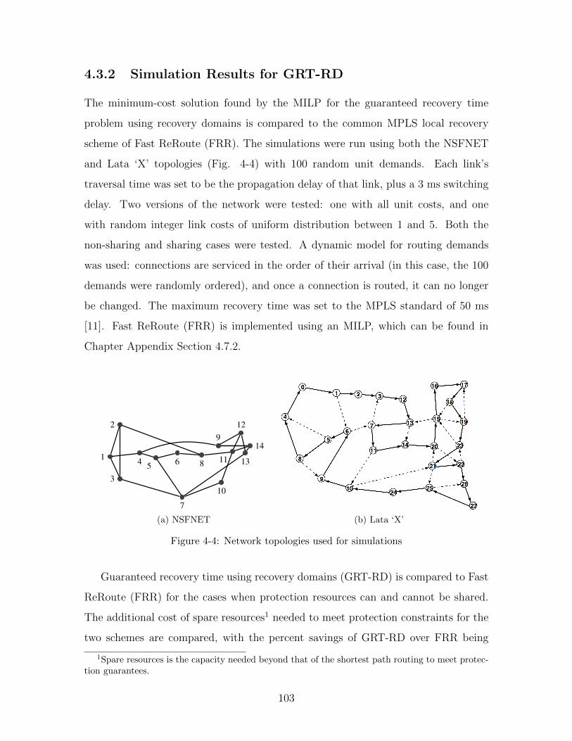
4.3.2 Simulation Results for GRT-RD

The minimum-cost solution found by the MILP for the guaranteed recovery time

problem using recovery domains is compared to the common MPLS local recovery

scheme of Fast ReRoute (FRR). The simulations were run using both the NSFNET

and Lata ‘X’ topologies (Fig. 4-4) with 100 random unit demands. Each link’s

traversal time was set to be the propagation delay of that link, plus a 3 ms switching

delay. Two versions of the network were tested: one with all unit costs, and one

with random integer link costs of uniform distribution between 1 and 5. Both the

non-sharing and sharing cases were tested. A dynamic model for routing demands

was used: connections are serviced in the order of their arrival (in this case, the 100

demands were randomly ordered), and once a connection is routed, it can no longer

be changed. The maximum recovery time was set to the MPLS standard of 50 ms

[11]. Fast ReRoute (FRR) is implemented using an MILP, which can be found in

Chapter Appendix Section 4.7.2.

2

1

3

4 5 6

7

8

9

10

11

12

13

14

Fig. 2: 14 Node NSFNET backbone network 100

120

140

160

180

200

220

240

260

280

0 0.25 0.5 0.75 1

Co

st

q

1+1 1+q LP DSPP

Fig. 3: Capacity cost vs. q for dynamic arrivals

protect for the failure of another edge, then that edge’s backup capacity can be shared. This model can be extended topartial protection by guaranteeing that any particular demand has its partial flow requirement met after a failure.

For the case of one-at-a-time routing, previous works offer heuristics to jointly optimize the primary and backup pathfor each incoming demand, as was done in both [2] and [3]. We instead choose a simple strategy of using the shortestpath for the primary. Our simulations show that using the shortest path for the primary route actually performs betterthan jointly optimizing the primary and backup paths for each incoming demand; the reason this occurs is discussedat the end of the section. We call our algorithm Dynamic Shared Partial Protection (DSPP).

We compare, via simulation, DSPP to 1 + 1, 1 + q and the LP, each of which jointly optimizes the primary andbackup paths for each incoming demand. Demands arrive dynamically and are served one-at-a-time in the order oftheir arrival. Performance of the strategies is compared using the NSFNET topology (Fig. 2) with 100 random unitdemands The protection requirement, q, for each demand is a truncated normal distribution with a standard deviation = 1

2 . The mean of q is varied between 0 and 1 for each iteration.The costs to route the demand and protection capacity are plotted in Fig. 3 as a function of the expected value of

q. It is seen that the partial protection scheme offers significant savings over 1 + 1 routing over a wide range of q,with the LP achieving even greater gains than 1+ q protection because of its use of flow bifurcation. With dynamicarrivals, we find that DSPP performs better than the schemes that jointly optimize the primary and backup paths. Thiscan be explained by observing that the algorithm takes the simple strategy of the shortest path as the primary for eachconnection, as opposed to jointly optimizing the primary and backup routes, which may take a longer primary pathto take advantage of backup sharing. The longer path makes it potentially more difficult for future demands to finddisjoint primary routes, lowering their ability to share protection resources. While other works have focused on findingheuristics to jointly optimize the primary and backup paths for each incoming demand, it appears a better approach isto simply take the shortest path for the primary route.

4. Conclusion

In this paper, a novel protection scheme to provide shared partial protection for a multi-commodity setting was in-troduced. A reduced complexity algorithm (DSPP) was developed, and for dynamic arrivals, DSPP actually performsbetter than jointly optimizing the primary and backup paths for each incoming demand.

References[1] S. Ramamurthy, L. Sahasrabuddhe, and B. Mukherjee, “Survivable WDM Mesh Networks,” Journal of Lightwave Technology 21, 870 (2003).

[2] C. Ou, J. Zhang, H. Zang, L. Sahasrabuddhe, and B. Mukherjee, “New and Improved Approaches for Shared-Path Protection in WDM MeshNetworks,” Journal of Lightwave Technology 22 (2004).

[3] G. Mohan, S. Murthy, and A. Somani, “Efficient algorithms for routing dependable connections in WDM optical networks,” Networking,IEEE/ACM Transactions on 9, 553–566 (2002).

[4] W. Grover, Mesh-Based Survivable Networks: Options and Strategies for Optical, MPLS, SO N E T, and ATM Networking (Prentice Hall, 2004).

[5] O. Gerstel and G. Sasaki, “Quality of Protection (QoP): a Quantitative Unifying Paradigm to Protection Service Grades,” Optical NetworksMagazine 3, 40–49 (2002).

[6] G. Kuperman, E. Modiano, and A. Narula-Tam, “Analysis and algorithms for partial protection in mesh networks,” in “INFOCOM, 2011Proceedings IEEE,” (IEEE, 2011), pp. 516–520.

[7] G. Kuperman, E. Modiano, and A. Narula-Tam, “Partial Protection in Networks with Backup Capacity Sharing,” Tech. rep., MIT,http://web.mit.edu/gregk/www/papers/PPNBCS.pdf (2011).

(a) NSFNET (b) Lata ‘X’

Figure 4-4: Network topologies used for simulations

Guaranteed recovery time using recovery domains (GRT-RD) is compared to Fast

ReRoute (FRR) for the cases when protection resources can and cannot be shared.

The additional cost of spare resources1 needed to meet protection constraints for the

two schemes are compared, with the percent savings of GRT-RD over FRR being

1Spare resources is the capacity needed beyond that of the shortest path routing to meet protec-tion guarantees.

103

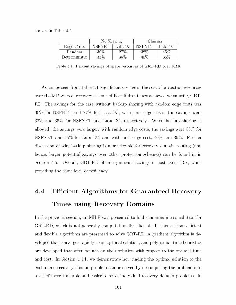
shown in Table 4.1.

No Sharing Sharing

Edge Costs NSFNET Lata ‘X’ NSFNET Lata ‘X’

Random 30% 27% 38% 45%Deterministic 32% 35% 40% 36%

Table 4.1: Percent savings of spare resources of GRT-RD over FRR

As can be seen from Table 4.1, significant savings in the cost of protection resources

over the MPLS local recovery scheme of Fast ReRoute are achieved when using GRT-

RD. The savings for the case without backup sharing with random edge costs was

30% for NSFNET and 27% for Lata ’X’; with unit edge costs, the savings were

32% and 35% for NSFNET and Lata ’X’, respectively. When backup sharing is

allowed, the savings were larger: with random edge costs, the savings were 38% for

NSFNET and 45% for Lata ’X’, and with unit edge cost, 40% and 36%. Further

discussion of why backup sharing is more flexible for recovery domain routing (and

hence, larger potential savings over other protection schemes) can be found in in

Section 4.5. Overall, GRT-RD offers significant savings in cost over FRR, while

providing the same level of resiliency.

4.4 Efficient Algorithms for Guaranteed Recovery

Times using Recovery Domains

In the previous section, an MILP was presented to find a minimum-cost solution for

GRT-RD, which is not generally computationally efficient. In this section, efficient

and flexible algorithms are presented to solve GRT-RD. A gradient algorithm is de-

veloped that converges rapidly to an optimal solution, and polynomial time heuristics

are developed that offer bounds on their solution with respect to the optimal time

and cost. In Section 4.4.1, we demonstrate how finding the optimal solution to the

end-to-end recovery domain problem can be solved by decomposing the problem into

a set of more tractable and easier to solve individual recovery domain problems. In

104

Section 4.4.2, a gradient algorithm using Lagrangian relaxation is developed, which

simulations show converges rapidly to an optimal solution. In Section 4.4.3, poly-

nomial timed heuristics that offer bounds with respect to the optimal solution are

presented. The different algorithms developed are compared to the optimal solution

found by the MILP in Section 4.4.4. Since it is NP-hard to simply determine if a

feasible solution exists for the guaranteed protection problem when backup sharing is

used [18], we first consider the case without backup sharing. Recovery domain routing

that guarantees recovery times with the use of backup capacity sharing is examined

in Section 4.5.

4.4.1 Decomposing the End-to-End Recovery Domain Prob-

lem

An optimal end-to-end recovery domain routing requires optimizing across the set of

possible recovery domains such that a flow from the source to destination is found

where the maximum amount of time the flow can be interrupted after a failure is

guaranteed. Each individual recovery domain is wholly responsible for protecting

against a failure between its respective end-points, and for ensuring that recovery

time guarantees are met. This requirement not only allows for easier rerouting after

a failure, but, as we demonstrate, allows the end-to-end problem to be simplified by

considering only the more tractable individual recovery domains.

The key observation that allows flexibility for finding a solution is that each pair

of nodes in the network marks the end-points of a potential recovery domain. Since

an end-to-end recovery domain routing will be a series of recovery domains connected

via their end-points, the optimal solution will be the lowest cost subset of individual

recovery domains that form a flow from the source to the destination. We note that

there are O(|V |2) potential recovery domains in a network.

Consider the network G in Fig. 4-5a, with link traversal times as labeled (in ms),

and unit cost links. We wish to find a minimum-cost recovery domain routing from

node s to d, with a maximum recovery time of 50 ms. For each pair of nodes in the

network, a minimum-cost recovery domain is found. A new network GR is constructed

105

s

15

15 15

15 15 15

25

25 a

b

c

d

(a) Original network G

s

a

b c

d

(b) Transformed network GR

Figure 4-5: Decomposing G into its individual recovery domains

with the same set of nodes as the original network G, and with an edge being placed

between any two nodes i and j if there exists a recovery domain between those nodes

that meets recovery time guarantees. The cost of all the edges that comprise the

recovery domain between nodes i and j is the cost of edge {i, j} in GR.

The graph transformation GR is shown in Fig. 4-5b. An edge between a pair of

nodes represents a recovery domain between those same two nodes in G that meets

recovery time guarantees. For example, edge {s, a} in GR has a cost of 3, and is a

recovery domain consisting of the following edge in G: {s, a}, {s, b}, and {b, a}. It is

easy to verify that for this example, each link in GR has a cost of 3. A shortest path

is found in GR from the source s to the destination d, where each edge of that path

represents a recovery domain that is used in the optimal end-to-end recovery domain

solution. The shortest path from s to d in GR is {s, b} and {b, d}, which represents

the recovery domains in G between s and b (consisting of the edges {s, a}, {a, b}, and

{s, b} in G), and b and d (consisting of the edges {b, c}, {c, d}, and {b, d} in G).

This algorithm is labeled end to end RD. We note that this approach does not

preclude two recovery domains from sharing edges between them, but the essence of

recovery domain routing is preserved: the end-nodes of a recovery domain maintain

full responsibility for protecting against a failure for the primary flow contained within

it, and for guaranteeing that the amount of time that flow can be interrupted does not

exceed the maximum allowed. This allows us to now focus on solving the individual

recovery domain problem, i.e., for a given a pair of nodes, finding the shortest-pair

of disjoint paths between those nodes that meet time constraints. With such an

106

algorithm at hand, one can use the above approach to solve for the end-to-end recovery

domain routing with guaranteed recovery times.

4.4.2 Optimal Algorithm

In this section, an optimal algorithm using a Lagrangian relaxation is presented. The

individual recovery domain problem is first formulated as an MILP, where we wish to

find a minimum-cost pair of disjoint paths between a source s and destination d that

have some maximum total link traversal time. The MILP is formulated as such: the

objective is to find a routing of minimum cost, such that two units of flow are routed

between the end-nodes s and d, with flow variables xij being binary, and the total

link traversal time not exceeding the maximum recovery time of T . Since an edge

will have strictly a flow of 0 or 1, two paths between s and d cannot overlap; hence,

a minimum-cost pair of disjoint paths will be found subject to the time constraints.

We refer to this as the constrained shortest-pair of disjoint paths problem.


cijxij (4.8)

∑{i,j}∈E

xij −∑{j,i}∈E

xji =

2 if i = s

−2 if i = d

0 o.w.

, ∀i ∈ V (4.9)

∑{i,j}∈E

tijxij ≤ T (4.10)

xij ∈ {0, 1}, ∀{i, j} ∈ E (4.11)

The Lagrangian dual is obtained by relaxing the maximum recovery time con-

107

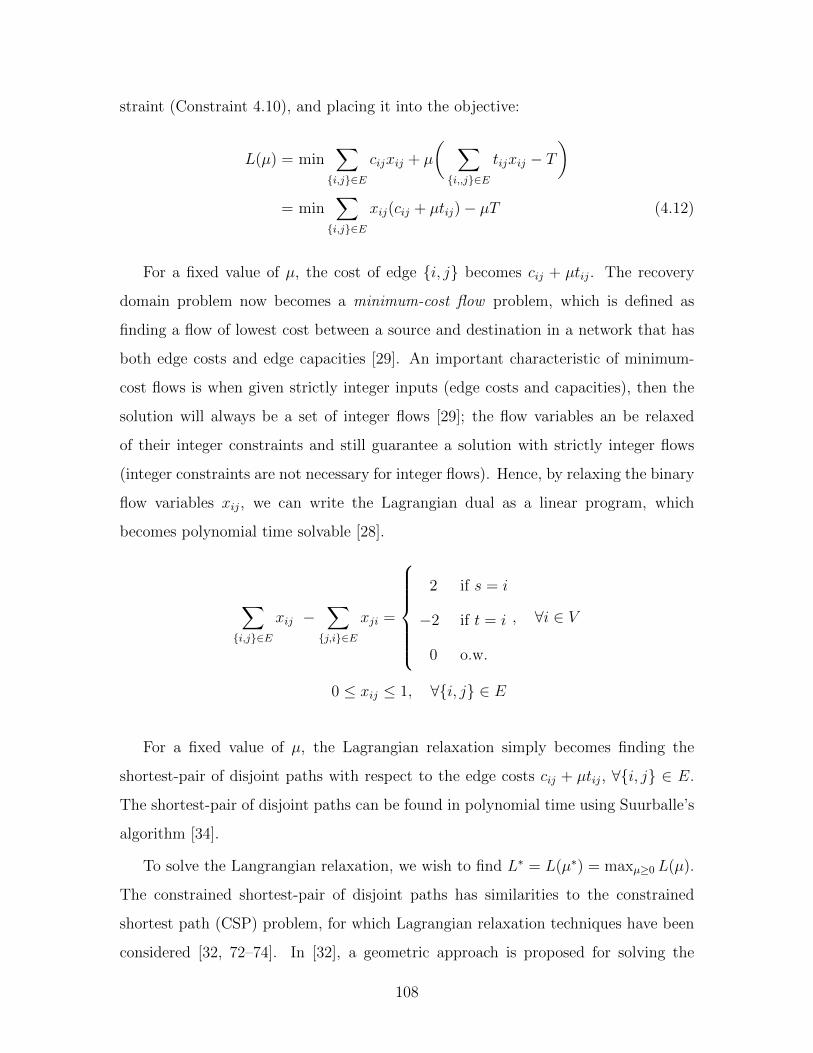
straint (Constraint 4.10), and placing it into the objective:

L(µ) = min∑{i,j}∈E

cijxij + µ

( ∑{i,,j}∈E

tijxij − T)

= min∑{i,j}∈E

xij(cij + µtij)− µT (4.12)

For a fixed value of µ, the cost of edge {i, j} becomes cij + µtij. The recovery

domain problem now becomes a minimum-cost flow problem, which is defined as

finding a flow of lowest cost between a source and destination in a network that has

both edge costs and edge capacities [29]. An important characteristic of minimum-

cost flows is when given strictly integer inputs (edge costs and capacities), then the

solution will always be a set of integer flows [29]; the flow variables an be relaxed

of their integer constraints and still guarantee a solution with strictly integer flows

(integer constraints are not necessary for integer flows). Hence, by relaxing the binary

flow variables xij, we can write the Lagrangian dual as a linear program, which

becomes polynomial time solvable [28].

∑{i,j}∈E

xij −∑{j,i}∈E

xji =

2 if s = i

−2 if t = i

0 o.w.

, ∀i ∈ V

0 ≤ xij ≤ 1, ∀{i, j} ∈ E

For a fixed value of µ, the Lagrangian relaxation simply becomes finding the

shortest-pair of disjoint paths with respect to the edge costs cij + µtij, ∀{i, j} ∈ E.

The shortest-pair of disjoint paths can be found in polynomial time using Suurballe’s

algorithm [34].

To solve the Langrangian relaxation, we wish to find L∗ = L(µ∗) = maxµ≥0 L(µ).

The constrained shortest-pair of disjoint paths has similarities to the constrained

shortest path (CSP) problem, for which Lagrangian relaxation techniques have been

considered [32, 72–74]. In [32], a geometric approach is proposed for solving the

108

L

μ μ*

L*

Figure 4-6: Pair of disjoint paths mapped to lines in L− µ space

Lagrangian relaxation for CSP. While not considered beyond a single constrained

path, we demonstrate that the geometric approach can be extended to the con-

strained shortest-pair of disjoint paths problem. L(µ) can be rewritten as L(µ,x) =

f(x) +µg(x), where f(x) =∑{i,j}∈E cijxij and g(x) =

∑{i,j}∈E tijxij −T . Each path

becomes a line in L−µ geometric space, where g(x) is the slope of the line, and f(x)

is the L axis crossing point. Furthermore, since g(x) =∑{i,j}∈E tijxij − T , the paths

associated with g(x) ≤ 0 meets time requirements, where f(x) is the cost of those

disjoint paths.

We see that the mapping to a geometric space is in fact not specific to CSP; any

discrete optimization problem that takes the form L(µ,x) = f(x) + µg(x) can be

represented as a line in L− µ space. In our case, each pair of disjoint paths becomes

a line in L− µ space, and the lower envelope of lines gives the optimal value for µ∗.

A visualization is shown in Fig. 4-6 [74].

Since any discrete optimization problem taking the form of L(µ,x) = f(x)+µg(x)

can be represented in geometric space, including the constrained shortest-pair of

disjoint paths, a similar method for finding the optimal µ∗ as in [32] can be applied.

The key is being able to solve for the optimal discrete variable assignments x for a

fixed µ in polynomial time. In the case of constrained shortest-pair of disjoint paths,

Suurballe’s algorithm [34] can be used, as previously discussed. The algorithm to find

the dual optimal solution is labeled rd dual opt, and is presented in Algorithm 1.

109

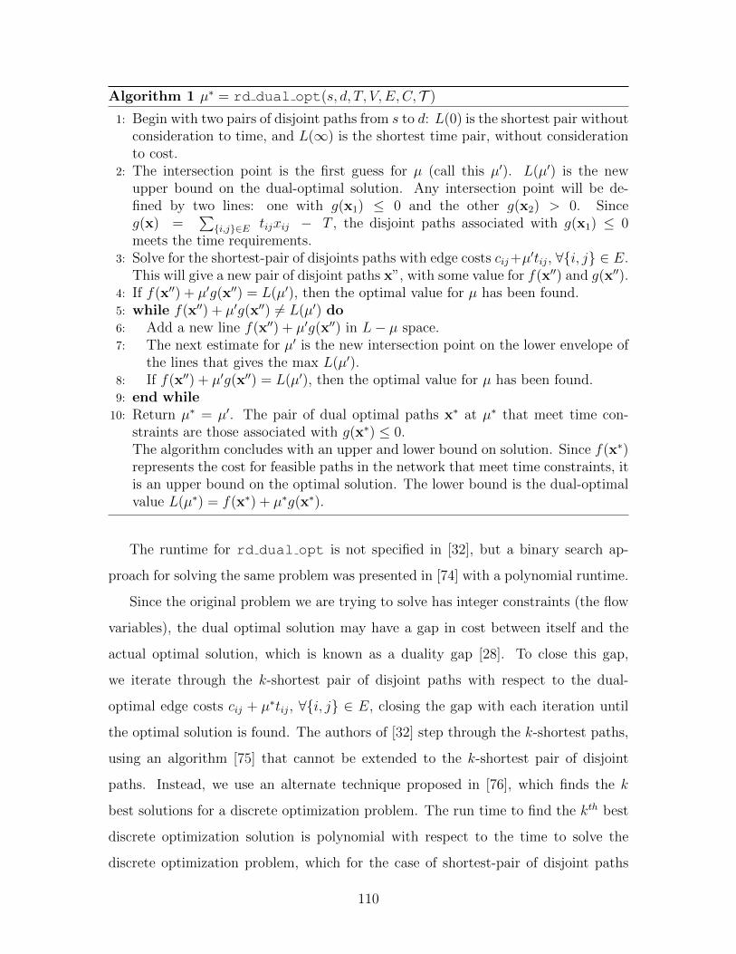
Algorithm 1 µ∗ = rd dual opt(s, d, T, V, E, C, T )

1: Begin with two pairs of disjoint paths from s to d: L(0) is the shortest pair withoutconsideration to time, and L(∞) is the shortest time pair, without considerationto cost.

2: The intersection point is the first guess for µ (call this µ′). L(µ′) is the newupper bound on the dual-optimal solution. Any intersection point will be de-fined by two lines: one with g(x1) ≤ 0 and the other g(x2) > 0. Sinceg(x) =

∑{i,j}∈E tijxij − T , the disjoint paths associated with g(x1) ≤ 0

meets the time requirements.3: Solve for the shortest-pair of disjoints paths with edge costs cij+µ

′tij, ∀{i, j} ∈ E.This will give a new pair of disjoint paths x”, with some value for f(x′′) and g(x′′).

4: If f(x′′) + µ′g(x′′) = L(µ′), then the optimal value for µ has been found.5: while f(x′′) + µ′g(x′′) 6= L(µ′) do6: Add a new line f(x′′) + µ′g(x′′) in L− µ space.7: The next estimate for µ′ is the new intersection point on the lower envelope of

the lines that gives the max L(µ′).8: If f(x′′) + µ′g(x′′) = L(µ′), then the optimal value for µ has been found.9: end while

10: Return µ∗ = µ′. The pair of dual optimal paths x∗ at µ∗ that meet time con-straints are those associated with g(x∗) ≤ 0.The algorithm concludes with an upper and lower bound on solution. Since f(x∗)represents the cost for feasible paths in the network that meet time constraints, itis an upper bound on the optimal solution. The lower bound is the dual-optimalvalue L(µ∗) = f(x∗) + µ∗g(x∗).

The runtime for rd dual opt is not specified in [32], but a binary search ap-

proach for solving the same problem was presented in [74] with a polynomial runtime.

Since the original problem we are trying to solve has integer constraints (the flow

variables), the dual optimal solution may have a gap in cost between itself and the

actual optimal solution, which is known as a duality gap [28]. To close this gap,

we iterate through the k-shortest pair of disjoint paths with respect to the dual-

optimal edge costs cij + µ∗tij, ∀{i, j} ∈ E, closing the gap with each iteration until

the optimal solution is found. The authors of [32] step through the k-shortest paths,

using an algorithm [75] that cannot be extended to the k-shortest pair of disjoint

paths. Instead, we use an alternate technique proposed in [76], which finds the k

best solutions for a discrete optimization problem. The run time to find the kth best

discrete optimization solution is polynomial with respect to the time to solve the

discrete optimization problem, which for the case of shortest-pair of disjoint paths

110

is also polynomial [34]. Details of the algorithm are omitted for brevity, and can be

found in [76]. We label the final algorithm, which closes the duality gap, rd opt; it

is presented in Algorithm 2.

Algorithm 2 (P1, P2) = rd opt(s, d, T, V, E, C, T )

1: Find the initial dual optimal solution:µ∗ = rd dual opt(s, d, T, V, E, C, T )

2: Find the kth shortest pair of disjoint paths xk for each k = 1, 2, ... with respectto the dual-optimal edge costs cij + µ∗tij.

• For each k, L(µ∗,xk) is the new lower bound on the optimal feasible solution,and is a non-decreasing function with respect to k.

• An upper bound Uk is maintained: Uk = min1..kf(xk) for all xk such thatg(xk) ≤ 0 (which means that xk is a solution that meets time constraints).Uk is a non-increasing upper bound.

3: Continue until Uk ≤ L(µ∗,xk), at which point the optimal solution has beenfound.

• Since we individually step through the shortest-pair of dual-optimal disjointpaths, which are a lower bound on the solution, until their cost is greaterthan the upper bound, which is a feasible solution, the solution must beoptimal. Proof is shown in [32].

4: Return the pair of disjoint paths P1 and P2 associated with the upper bound Uk,which meets time constraints.

Since the number of possible disjoint paths can be potentially exponential with

respect to the number of edges, the number of iterations to close the duality gap is not

necessarily polynomial bounded. But, our simulations indicate that the number of

iterations to close the duality gap is in fact minimal: on average, only 1.46 iterations

are needed.

4.4.3 Polynomial Timed Heuristics

In this section, two algorithms are presented that run in polynomial time to solve

the guaranteed recovery time problem using recovery domains. The first is a “fastest

paths” algorithm, where link costs are ignored, and paths are found with respect to

time only. This algorithm is the simplest to implement, and is most useful when link

111

costs are either not considered, or are proportional to the link traversal times. The

second is a fully polynomial time approximation scheme (FPTAS) that guarantees a

solution to be within a factor of 1.5 of the optimal cost and 1.5(1+ε) of the maximum

recovery time.

The fastest paths algorithm is straightforward to implement using the shortest-

pair of disjoint paths algorithm [34]. Instead of finding a pair of disjoint paths of

minimum-cost, a pair of disjoint paths of minimum time are found. This algorithm

is called rd fastest, and has the same complexity as finding the shortest-pair of

disjoint paths.

For the approximation scheme, we use an algorithm presented in [57]. In that

work, the authors try to solve for disjoint QoS (quality-of-service) paths, such that

each path is bounded by some time requirement D. They are not looking at recovery

times or recovery domains, but are instead interested in ensuring that the end-to-

end primary and backup paths do not exceed some QoS specification. To solve their

problem, they relax each path’s individual time constraint and try to find a pair of

disjoint paths such that the sum of the link traversal times for both paths does not

exceed 2D. By replacing the time requirement 2D with the maximum recovery time

requirement T , we can solve for a recovery domain with a bound on the optimal

cost and time. We label this approximation algorithm rd approx; details of the

algorithm are omitted for brevity, and can be found in [57].

4.4.4 Algorithm Simulations

In this section, the algorithms developed in the previous sections for guaranteed re-

covery times using recovery domains are compared to the end-to-end optimal solution

found by the MILP from Section 4.3. A similar simulation to Section 4.3.2 was run,

using the Lata ‘X’ topology (Fig. 4-4b). Table 4.2 shows the percent that each of

the algorithms differed in total cost of resources used over the minimum-cost solution

found by the MILP.

As expected, the optimal algorithm rd opt did not differ from the optimal so-

lution found by the MILP. Additionally, the average number of iterations needed to

112

Protection Scheme Unit Edge Costs Random Edge Costs

rd opt 0 0rd fastest 1% 6%rd approx 5% 2%

Table 4.2: Difference for the algorithms from optimal

close the duality gap was 1.46 over all simulated demands. Both the fastest paths

and approximation algorithm also performed close to optimal. When edge costs were

uniform, the fastest paths approach in fact gave slightly better results. But when

edge costs were changed to be random, the approximation algorithm performed bet-

ter since it tries to optimize with respect to cost, and the fastest paths algorithm does

not.

4.5 Algorithm with Backup Capacity Sharing

In the previous section, efficient algorithms that offer bounds with respect to the

optimal solution were presented without the use of backup capacity sharing. These

results are useful for a basic understanding of the guaranteed recovery time problem

using recovery domains (GRT-RD), and for networks that do not allow protection

sharing. But many times, networks do utilize backup sharing, and significant savings

can often be achieved. In this section, a time-efficient algorithm for GRT-RD using

backup capacity sharing is presented.


then under a single-link failure model, at most one can be disrupted at any given point

in time. Since at most one demand will need to be restored after a failure, two failure-

disjoint flows can share backup capacity. An interesting feature of recovery domain

routing is that two demands can share backup capacity even if their two primary flows

are not failure disjoint. Traditionally, in path protection schemes, two paths can only

share protection resources if their primary paths are disjoint. However, in the recovery

domain setting, sharing can take place between two recovery domains, so long as the

primary segments in those recovery domains are disjoint. Thus, end-to-end primary

113

paths that are not entirely disjoint may still share backup resources.

1 2 3

4

5

p1, p2 b1, b2

b1

b2

p1

p2

b1

b2

Figure 4-7: Sharing protection resources in a recovery domain

An example of an end-to-end recovery domain routing for two demands is shown

in Fig. 4-7. Demand 1 is routed from node 1 to node 4, and demand 2 is routed from

node 1 to node 5. The primary paths are labeled p1 and p2 for demands 1 and 2,

respectively, and backup paths are labeled b1 and b2. Two recovery domains are used

for each demand: demand 1 uses recovery domains with the end-points of (1, 2), and

(2, 4); demand 2 uses recovery domains with the end-points of (1, 2), and (2, 5). The

two primary paths overlap in the first recovery domain on the path segment between

nodes 1 and 2; hence, they cannot share protection resources within that domain, and

each demand has its own dedicated backup path. The primary segments for the two

recovery domains starting at node 2 and going to their respective destinations are

failure disjoint. Even though the two primary paths overlap between nodes 1 and 2,

the two demands can share protection resources for their recovery domains after node

2. On the path segment between nodes 2 and 3, only one unit of backup capacity

allocation is needed to protect against a failure for either demand’s primary path in

recovery domains (2, 4) or (2, 5).

Since a failure is local to a recovery domain, and the primary flow outside of that

recovery domain is not affected, a similar approach can be used as was done previously

for the algorithms without backup capacity sharing: for every pair of nodes, we

find the recovery domain routing that guarantees recovery time and utilizes backup

capacity sharing. Then, an end-to-end recovery domain routing is constructed from

114

a subset of those recovery domains using end to end RD (Section 4.4.1).

Conflict sets are used to determine how much backup capacity can be shared

by each incoming demand [18]. A conflict set indicates how much backup sharing is

possible on an edge by examining how much backup capacity it already has to protect

against any particular edge failure. If some edge has more backup capacity already

assigned to it than is needed to protect against a particular edge failure, then those

resources can be used at no additional cost. For example, let some edge {i, j} have

one unit of backup capacity allocated to it to protect against the failure of {k, l},

and with edge {i, j} not being scheduled to protect against any other link failures.

Now consider some new connection with a primary flow that uses some other edge

{u, v}. Edges {k, l} and {u, v} can never fail simultaneously under a single-link failure

model; thus, the new connection can use the backup capacity allocated to {i, j} for

protecting against the failure of {u, v} without incurring additional cost. Further

details of protection routing using conflict sets can be found in [18].

We consider routing demands dynamically (one-at-a-time), where once a connec-

tion is routed, it can no longer be changed; this model is similar to those used in

path protection schemes [18, 68]. These path protection schemes offer heuristics to

jointly optimize the primary and backup path for each incoming demand. We instead

choose the simple strategy of using the shortest path for the primary route. After

the primary path is found, the cost to use the remaining edges to protect that path

can be determined (i.e., find out if edges can utilize protection resource sharing at

no additional cost). If the maximum recovery time is T , and the shortest path has

traversal time ts, then a backup path is a constrained shortest path (CSP) that has

a traversal time of at most (T − ts). To solve for the CSP, an optimal solution can

be found in pseudo-polynomial time [56]; if T is rational and polynomial bounded

with respect to the input parameters, the algorithm becomes polynomial. We label

this algorithm rd sharing. Our simulations show that using the shortest path for

the primary route in fact performs better than jointly optimizing the primary and

backup paths for each incoming demand.

To test the performance of rd sharing, a similar simulation to Section 4.3.2

115

Protection Scheme NSFNET Lata ‘X’

Local Recovery with Sharing 583 3459Greedy Optimal Recovery with Sharing 351 2677

End-to-end rd sharing 349 2605

Table 4.3: Cost of allocation for different protection schemes

was run. The simulations were run using both the NSFNET and Lata ‘X’ topologies

(Fig. 4-4) with 75 random unit demands. Each link’s traversal time was set to be the

propagation delay of that link, plus a 3 ms switching delay. Edges have random integer

cost with uniform distribution between 1 and 5, and the maximum recovery time is set

to the MPLS standard of 50 ms [11]. Three different schemes were tested: the optimal

recovery domain routing with sharing, which jointly optimizes the primary and backup

path for each incoming demand (using the MILP from Chapter Appendix Section

4.7.1), local recovery (FRR) with sharing (found in Chapter Appendix Section 4.7.2),

and the end-to-end rd sharing algorithm developed in this section. A dynamic

model was used: connections are serviced in the order of their arrival, and once a

connection is routed, it can no longer be changed. Table 4.3 shows the total cost

of allocation needed to route all 75 demands using the aforementioned protection

schemes.

As anticipated, the optimal recovery scheme performs better than the local re-

covery scheme. Interestingly, the end-to-end rd sharing algorithm performs better

than the supposed optimal recovery with sharing. This can be explained by observ-

ing that the algorithm takes the simple strategy of the shortest path as the primary

for each connection. This is as opposed to the optimal recovery scheme that jointly

optimizes the primary and backup routes for each incoming demand, which may take

a longer primary path to take advantage of backup sharing. By greedily optimizing

every incoming demand, the potentially longer primary path makes it more diffi-

cult for future demands to find failure disjoint routes, lowering their ability to share

protection resources, and thus increasing the overall cost.

116

4.6 Conclusion

In this chapter, we examined the problem of providing network protection with guar-

anteed recovery times using recovery domains (GRT-RD). The network is partitioned

into failure-independent “recovery domains”, where within each domain, the time to

recover from a failure is guaranteed. To meet these guarantees, we provide an opti-

mal solution in the form of an MILP. We demonstrate that the network-wide optimal

solution can be decomposed into a set of more tractable and easier to solve subprob-

lems. This allows for the development of flexible and efficient solutions, including an

optimal algorithm using Lagrangian relaxation, which simulations show to converge

rapidly to an optimal solution. Low complexity heuristics are developed for both with

and without backup sharing. For dynamic arrivals, the algorithm utilizing backup

sharing and using shortest paths performs better than the solution that greedily tries

to optimize for each incoming demand.


4.7.1 Guaranteed Recovery Time using Recovery Domains

with Backup Capacity Sharing


• V is the set of vertices, and E is the set of edges

• f sd is the amount of flow that need to be routed from s to d, assumed to be

integer


• tij is the traversal time for link {i, j}

• T is the maximum recovery time


117

• xstij is 1 if flow is assigned on link {i, j} or demand (s, t), and 0 o.w.

• pstij,kl is 1 if protection flow is assigned on link {i, j} after the failure of link {k, l}

for demand (s, t), and 0 o.w.

• ystij,kl is 1 if spare capacity is assigned on on link {i, j} for failure of link {k, l}

for demand (s, t) , and 0 o.w.

• wij is total primary flow on link {i, j}, wij ≥ 0

• sij is total spare allocation on link {i, j}, sij ≥ 0

• Rsdkl is 1 if the recovery domain with end nodes k and l for demand (s, d) is

active (part of the solution), 0 o.w.

• rsdij,kl is 1 if link {i, j} is in recovery domain (k, l) for demand (s, d), 0 o.w.

The objective is to:

• Minimize the cost of allocation over all links:

min∑{i,j}∈E



• Route primary traffic between s and d:

∑{i,j}∈E

xsdij −∑{j,i}∈E

xsdji =

1 if i = s

−1 if i = d

0 o.w.

, ∀i∈V∀(s,d)∈(V,V ) (4.14)

• Route flow to protect after the failure of link {k, l}:

∑{i,j}∈E{i,j}6={k,l}

psdij,kl −∑{j,i}∈E{j,i}6={k,l}

psdji,kl =

1 if i = s

−1 if i = d

0 o.w.

, ∀i∈V, ∀{k,l}∈E∀(s,d)∈(V,V ) (4.15)

118

• Primary capacity on link {i, j} must meet all primary flows before a link failure

∑(s,d)∈(V,V )

f sdxsdij ≤ wij, ∀{i, j} ∈ E (4.16)

• Primary and spare capacity on link {i, j} must be sufficient for all protection

flows after failure of link {k, l}:

psdij,kl ≤ xsdij + ysdij,kl,∀{i,j}∈E, ∀{k,l}∈E∀(s,d)∈(V,V ) (4.17)

• Spare capacity on link {i, j} satisfies all protection flows after failure of link

{k, l}:

∑(s,d)∈(V,V )

f sdysdij,kl ≤ sij,∀{i,j}∈E∀{k,l}∈E (4.18)

• Mark active recovery domains

– If any edge in a recovery domain is active, then that recovery domain is

active

∑{i,j}∈E

rsdij,kl ≤ |E| ·Rsdkl ,

∀(k,l)∈(V,V )∀(s,d)∈(V,V ) (4.19)

– If no edge in a recovery domain is active, then that recovery domain is not

active

∑{i,j}∈E

rsdij,kl ≥ Rsdkl ,

∀(k,l)∈(V,V )∀(s,d)∈(V,V ) (4.20)

• For each active recovery domain, find two disjoint paths between its respective

119

end nodes k and l

∑{i,j}∈E

rsdij,kl −∑{j,i}∈E

rsdji,kl =

2Rsd

kl if i = k

−2Rsdkl if i = l

0 o.w.

, ∀i∈V, (k,l)∈(V,V )∀(s,d)∈(V,V ) (4.21)

• The sum of the traversed time delays of the edges in a given recovery domain

cannot exceed the maximum recovery time

∑{i,j}∈E

rsdij,kltij ≤ T, ∀(k,l)∈(V,V )∀(s,d)∈(V,V ) (4.22)

4.7.2 MILP for Optimal Local Recovery (Fast ReRoute)

The following is an MILP for optimal local recovery for a single demand requiring

unit flow. Sharing can be accomplished by using similar techniques as the MILP for

GRT-RD with sharing, shown in Chapter Appendix Section 4.7.1.


• V is the set of vertices and E is the set of edges


• (s, d) is the source and destination


• xij is 1 if primary flow is assigned to link {i, j}, and 0 otherwise

• f ijkl is 1 flow is assigned to link {i, j} to protect after the failure of link {k, l}, 0

otherwise

• sij is 1 if protection flow is assigned to link {i, j}, and 0 otherwise

120

The objective is to minimize the total cost of allocation:


cij(xij + sij) (4.23)


• Route primary traffic to meet demand before a failure

∑{i,j}∈E

xij −∑{j,i}∈E

xji =

1 if i = s

−1 if i = d

0 otherwise

, ∀i ∈ V (4.24)

• Route flow from point of local repair k to destination d after the failure of link

{k, l} if link {k, l} carried flow

∑j∈Vj 6=l

f ijkl −∑j∈Vj 6=l

f jikl = xkl, ∀{k, l} ∈ E (4.25)

∑j∈Vj 6=k

f jdkd −∑j∈Vj 6=k

f tjkd = −xkd, ∀{k, d} ∈ E (4.26)

∑{i,j}∈E{k,l}6={i,j}i 6=k∨d

f ijkl −∑{j,i}∈E{k,l}6={j,i}i 6=k∨d

f jikl = 0, ∀i∈V∀{k,l}∈E (4.27)

• Primary and spare capacity assigned on any link meets flow requirements after

the failure of link {k, l}

f ijkl ≤ xij + sij,∀{i,j}∈E∀{k,l}∈E (4.28)

121

Chapter 5

Providing Protection in Multi-Hop

Wireless Networks

In the previous chapters of this thesis, we investigated service guarantees for wired

networks. We now consider guaranteeing service in wireless networks that takes into

account the additional challenges of having interference-free communications across

a shared transmission space.

5.1 Introduction

Multi-hop wireless mesh networks have become increasingly ubiquitous, with wide-

ranging applications from military to sensor networks. As these networks continue

gaining in prominence, there is an increasing need to provide protection against node

and link failures. In particular, wireless mesh networks have recently emerged as a

promising solution for providing Internet access. Since these networks will be tightly

coupled with the wired Internet to provide Internet services to end-users, they must

be equally reliable. Wired networks have long provided pre-planned backup paths,

which offer rapid and guaranteed recovery from failures. These protection techniques

cannot be directly applied to wireless networks due to interference constraints. As

opposed to wired networks, two wireless nodes in close proximity will interfere with

one another if they transmit simultaneously in the same frequency channel. So, in

123

addition to finding a backup route, a schedule of link transmissions needs to be

specified. In this work, we consider the problem of providing guaranteed protection

in wireless networks with interference constraints via pre-planned backup routes, as

well as their corresponding link transmission schedules.

Guaranteed protection schemes for wired networks have been studied extensively

[2, 3, 5, 17, 18], with the most common scheme being 1+1 guaranteed path protection

[3]. The 1+1 protection scheme provides an edge-disjoint backup path for each work-

ing path, and guarantees the full demand to be available at all times after any single

link failure. Protection schemes optimized for wireless networks with interference con-

straints have not yet been considered. Typically, an approach for resiliency in wireless

networks (in particular sensor networks) is to ensure that there exists “coverage” for

all nodes given some set of link failures [78, 79]. This approach to resiliency does not

consider routing and scheduling with respect to interference constraints, and assumes

that there exists some mechanism to find a route and schedule at any given point in

time. Furthermore, there is no guarantee that sufficient capacity will be available to

protect against a failure. The idea of applying 1 + 1 protection in wireless networks

is briefly mentioned in [80]. However, [80] does not study the specific technical de-

tails of such an approach to wireless protection. The goal of this chapter is to study

protection mechanisms for wireless networks with a particular focus on the impact of

wireless interference and the need for scheduling.

The addition of interference constraints makes the protection problem in a wireless

setting fundamentally different from the ones found in a wired context. After a failure

in a wireless network, links that could not have been used due to interference with the

failed link become available, and can be used to recover from the failure. In fact, it

is often possible to add protection in a wireless setting without using any additional

resources.

Consider allocating a protection route for the following example, shown in Fig.

5-1. The wireless network operates in a time-slotted fashion, with equal length time

slots available for transmission. Any two nodes within transmission range have a

link between them, and each link’s time slot assignment is shown in the figures. We

124

s d

a

b

c

1

2 1

2

(a) Before a failure

s d

a

b

c

1

2 1

2

(b) After {s, b} fails

Figure 5-1: Time slot assignment for protection in a wireless network

assume a 1-hop interference model where any two links that have a node in common

cannot be active at the same time. Additionally, we assume unit capacity links.

Before any failure, the maximum flow from s to d is 1, and can be achieved using

a two time slot schedule, as shown in Fig. 5-1a. At any given point in time, only

one outgoing link from s can be active, and similarly, only one incoming link to d

can be active. Wireless links {s, c}, and {c, d} cannot be used prior to the failure

of {s, b}, but become available after {s, b} fails. After the failure of {s, b}, flow can

be routed from s to c during time slot 2, and from c to d during slot 1, as shown

in Fig. 5-1b. Similar schedules can be found for failures of the other links. The

maximum flow from s to d is 1 for both before and after a failure; i.e., there is no

reduction in maximum throughput when allocating resources for a protection route

on {s, c} and {c, d}: protection can be assigned for “free”. This is in contrast to a

wired network where the maximum throughput without protection from s to d is 3,

and the maximum throughput when assigning a protection route on {s, c} and {c, d}

is 2, which amounts to a 13

loss in throughput due to protection.

The novel contributions of this chapter is introducing the Wireless Guaranteed

Protection (WGP) problem in multi-hop networks with interference constraints. In

Section 5.2, the model for WGP is presented. In Section 5.3, properties of an optimal

solution are examined for a single demand with 1-hop interference constraints, which

are then used to motivate the development of a time-efficient algorithm. In Section

5.4, an optimal solution is developed via a mixed integer linear program for general

125

interference constraints. In Section 5.5, time-efficient algorithms are developed that

perform within 4.5% of the optimal solution.

5.2 Model and Problem Description

In this chapter, solutions to the guaranteed protection problem for multi-hop wireless

networks subject to interference constraints are developed and analyzed. Our goal is

to provide protection in a manner similar to what has been done in the wired setting.

Namely, after the failure of some network element, all connections must maintain the

same level of flow that they had before the failure. In order to do so, resources are

allocated and scheduled in advance on alternate (backup) routes to protect against

failures.

In wired networks, two adjacent nodes can transmit simultaneously because they

do not interfere with one another; if capacity exists on a set of links, a path can be

routed using that capacity. Wireless networks are different; interference constraints

must be considered. A set of links in close proximity cannot transmit simultaneously

on the same frequency channel; only one link from that set can be active at a time,

or else they will interfere with one another. Not only must a path between the

source and destination be found with available capacity, but also a schedule of link

transmissions needs to be determined. This is known as the routing and scheduling

problem [36, 80–87], which is known to be NP-Hard [36].

The addition of interference constraints adds complexity to the traditional wired

protection problem, but also presents an opportunity to gain protection from failures

with minimal loss of throughput. After a failure in a wireless network, links that could

not have been used due to interference with the failed link become available, and can

be used to recover from the failure. In fact, it is often possible to add protection in

a wireless setting without any loss in throughput.

The following network model is used for the remainder of the chapter. A graph G

has a set of vertices V and edges E. An interference matrix I is given, where Iklij ∈ I

is 1 if links {i, j} and {k, l} can be activated simultaneously (do not interfere with

126

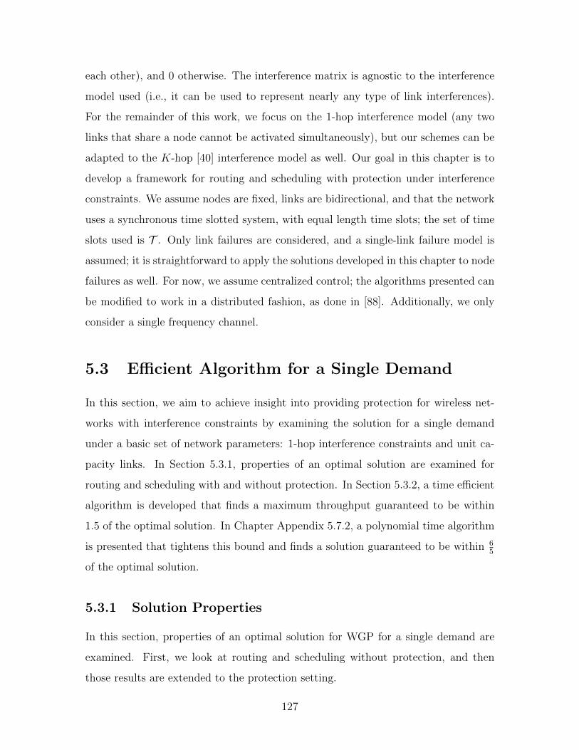
each other), and 0 otherwise. The interference matrix is agnostic to the interference

model used (i.e., it can be used to represent nearly any type of link interferences).

For the remainder of this work, we focus on the 1-hop interference model (any two

links that share a node cannot be activated simultaneously), but our schemes can be

adapted to the K-hop [40] interference model as well. Our goal in this chapter is to

develop a framework for routing and scheduling with protection under interference

constraints. We assume nodes are fixed, links are bidirectional, and that the network

uses a synchronous time slotted system, with equal length time slots; the set of time

slots used is T . Only link failures are considered, and a single-link failure model is

assumed; it is straightforward to apply the solutions developed in this chapter to node

failures as well. For now, we assume centralized control; the algorithms presented can

be modified to work in a distributed fashion, as done in [88]. Additionally, we only

consider a single frequency channel.

5.3 Efficient Algorithm for a Single Demand

In this section, we aim to achieve insight into providing protection for wireless net-

works with interference constraints by examining the solution for a single demand

under a basic set of network parameters: 1-hop interference constraints and unit ca-

pacity links. In Section 5.3.1, properties of an optimal solution are examined for

routing and scheduling with and without protection. In Section 5.3.2, a time efficient

algorithm is developed that finds a maximum throughput guaranteed to be within

1.5 of the optimal solution. In Chapter Appendix 5.7.2, a polynomial time algorithm

is presented that tightens this bound and finds a solution guaranteed to be within 65

of the optimal solution.

5.3.1 Solution Properties

In this section, properties of an optimal solution for WGP for a single demand are

examined. First, we look at routing and scheduling without protection, and then

those results are extended to the protection setting.

127

Lemma 5.1. The maximum flow that can be routed and scheduled between the source

s and destination d under 1-hop interference constraints without protection is 1.

Proof. Under 1-hop interference constraints, only one link exiting the source node

can be active at time. Since each link has unit capacity, the maximum flow that can

leave the source (or enter the destination) is 1.

While Lemma 5.1 indicates that a flow of 1 is possible, it does not necessarily

mean that a flow of 1 can be achieved. We note that if the source s and destination

d are adjacent, then a maximum flow of 1 can always be achieved by using one edge

between the two. We assume for the remainder of this section that s and d are at least

two hops apart. We now give the properties of maximum flows for a single demand

in a unit-capacity wireless network under 1-hop interference constraints.

Lemma 5.2. To achieve the maximum flow of 1, there must exist at least two node-

disjoint paths from s to d.

Proof. Assume otherwise: there are no node-disjoint paths, and there is a maximum

flow of 1 possible from s to d. If there are no node-disjoint paths between s and d,

then by Menger’s theorem there exists a single node j whose removal will separate

s and d [29]; hence, all paths from s to d must pass through j. In order for a flow

of 1 to exist between s and d, node j must have a total of 1 unit of flow coming in,

and 1 unit of flow going out. This is only possible if node j is both receiving and

transmitting the entire time, which is not possible under the 1-hop interference model

since node j cannot be both receiving and transmitting simultaneoulsy.

Corollary 5.1. If two node-disjoint paths from s to d do not exist, then the maximum

flow is 12.

Proof. In the proof for Lemma 5.2, it was shown that if no node-disjoint paths exist

between s and d, all paths must cross some node j. Node j cannot be receiving and

transmitting at the same time under the 1-hop interference model. The maximum

flow that j can support is to be recieving half of the time, and transmitting the other

128

half. Increasing the amount of time j is transmitting will reduce the amount of time

it can transmit, which reduces the overall flow. The same is seen if the amount of

time j is receiving is increased. Hence, j will have incoming flow half of the time,

and outgoing flow for the other half. Since each edge has unit capacity, the maximum

flow possible through node j is 12.

Any loop-free path from s to d (when s and d are greater than one hop apart from

one another) can have an interference-free schedule by alternating between time slots

1 and 2 for each edge of the path; hence, any edge of the path will only be active for

half of the time, and the path will support a flow of 12. If two or more node-disjoint

paths do exist, then a maximum flow is dependent on the total number of edges in

the disjoint paths.

Lemma 5.3. If there exists two node-disjoint paths between s and d with an even

total number of edges over both paths, then the maximum flow of 1 is achievable.

Proof. When both paths have an even total number of edges, an interference-free

schedule using two time slots is possible by alternating time slot assignments on each

path. If each path has an even number of edges, then path 1 will begin with time

slot 1 and end with time slot 2, and path 2 will begin with time slot 2 and end with

time slot 1. Each unit-capacity edge will be active for half of the time; hence, each

path carries a total of 12

unit of flow, giving the maximum flow of 1 using both paths.

A similar schedule can be shown for the case when each path has an odd number of

edges.

To help see Lemma 5.3, two examples are shown in Fig. 5-2, with the time slot

assignments for the links labeled in the figures. In Fig. 5-2a and 5-2b, there are two

node-disjoint paths from the source s to destination d that have an even total number

of edges. In Fig. 5-2a, each path has an even number of edges, and in Fig. 5-2b, each

path has an odd number of edges. An interference-free schedule for the two paths

can be found using two time slots. Each link is active for 12

of the time; hence, each

path can support a flow of 12, giving a total flow of 1 from s to d.

129

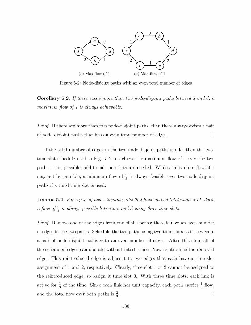
s d

a

b

1

2 1

2

(a) Max flow of 1

s d

a 1

2 b 1

c 2 1 e

2

(b) Max flow of 1

Figure 5-2: Node-disjoint paths with an even total number of edges

Corollary 5.2. If there exists more than two node-disjoint paths between s and d, a

maximum flow of 1 is always achievable.

Proof. If there are more than two node-disjoint paths, then there always exists a pair

of node-disjoint paths that has an even total number of edges.

If the total number of edges in the two node-disjoint paths is odd, then the two-

time slot schedule used in Fig. 5-2 to achieve the maximum flow of 1 over the two

paths is not possible; additional time slots are needed. While a maximum flow of 1

may not be possible, a minimum flow of 23

is always feasible over two node-disjoint

paths if a third time slot is used.

Lemma 5.4. For a pair of node-disjoint paths that have an odd total number of edges,

a flow of 23

is always possible between s and d using three time slots.

Proof. Remove one of the edges from one of the paths; there is now an even number

of edges in the two paths. Schedule the two paths using two time slots as if they were

a pair of node-disjoint paths with an even number of edges. After this step, all of

the scheduled edges can operate without interference. Now reintroduce the removed

edge. This reintroduced edge is adjacent to two edges that each have a time slot

assignment of 1 and 2, respectively. Clearly, time slot 1 or 2 cannot be assigned to

the reintroduced edge, so assign it time slot 3. With three time slots, each link is

active for 13

of the time. Since each link has unit capacity, each path carries 13

flow,

and the total flow over both paths is 23.

130

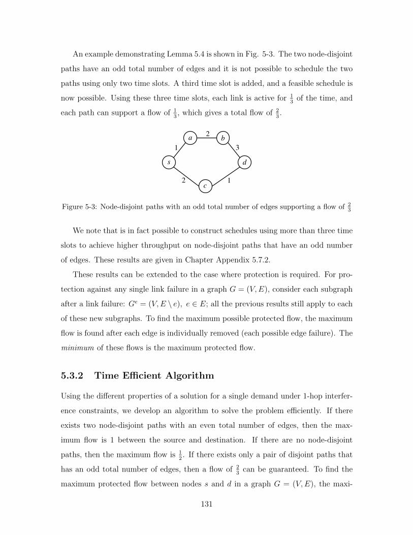
An example demonstrating Lemma 5.4 is shown in Fig. 5-3. The two node-disjoint

paths have an odd total number of edges and it is not possible to schedule the two

paths using only two time slots. A third time slot is added, and a feasible schedule is

now possible. Using these three time slots, each link is active for 13

of the time, and

each path can support a flow of 13, which gives a total flow of 2

3.

s d

a

c

1

2 1

2 b 3

Figure 5-3: Node-disjoint paths with an odd total number of edges supporting a flow of 23

We note that is in fact possible to construct schedules using more than three time

slots to achieve higher throughput on node-disjoint paths that have an odd number

of edges. These results are given in Chapter Appendix 5.7.2.

These results can be extended to the case where protection is required. For pro-

tection against any single link failure in a graph G = (V,E), consider each subgraph

after a link failure: Ge = (V,E \ e), e ∈ E; all the previous results still apply to each

of these new subgraphs. To find the maximum possible protected flow, the maximum

flow is found after each edge is individually removed (each possible edge failure). The

minimum of these flows is the maximum protected flow.

5.3.2 Time Efficient Algorithm

Using the different properties of a solution for a single demand under 1-hop interfer-

ence constraints, we develop an algorithm to solve the problem efficiently. If there

exists two node-disjoint paths with an even total number of edges, then the max-

imum flow is 1 between the source and destination. If there are no node-disjoint

paths, then the maximum flow is 12. If there exists only a pair of disjoint paths that

has an odd total number of edges, then a flow of 23

can be guaranteed. To find the

maximum protected flow between nodes s and d in a graph G = (V,E), the maxi-

131

mum flow is found for each link failure by using a subgraph with each link e removed:

Ge = (V,E \ e), e ∈ E. The minimum of these maximum flows is the maximum

protected flow possible for the demand.

The key to finding the maximum protected flow is to be able to identify node-

disjoint paths between s and d with either an even or odd total number of edges. If

there are at most two node-disjoint paths, then the maximum flow can only be found

if it is possible to find a pair of paths with an even total number of edges. Hence, we

focus on trying to find a pair of node-disjoint paths that have an even total number

of edges over both of the paths. There has been limited work on trying to identify

shortest paths with an even number of edges [89], but no work looking at such an

algorithm for disjoint paths.

Development of the optimal algorithm is as follows: we first find the shortest pair

of edge-disjoint paths with an even number of total edges, and then we extend this

algorithm to find the shortest pair of node-disjoint paths with an even number of

total edges.

Shortest pair of edge-disjoint paths with an even number of total edges

To find the shortest pair of edge-disjoint paths with an even number of edges, we

begin by considering the more general case without the even-edge restriction (the

paths can have any number of edges), which was previously considered in [34]. We

use a different formulation for the problem by using minimum-cost flows, which are

defined as finding a flow of minimum cost between a source and destination in a

network that has both edge costs and edge capacities [29]. Minimum-cost flows have

the property that when given all integer inputs (for edge costs and capacities), they

will have all integer solutions (integer flows). We solve the shortest disjoint pair of

paths problem by solving the following optimization problem: find a flow of minimum

cost to route two units from s to d in a graph with unit capacity and unit cost edges.

This will find the shortest pair of disjoint paths since two units of flow need to be

routed, no edge can have more than a single unit of flow, and with integer inputs,

the solution will be integer, which will be two edge-disjoint paths of unit flow and

132

minimum cost.

One algorithm to solve the minimum-cost flow problem is the successive shortest

paths (SSP) algorithm [29]. SSP finds the shortest path, and routes the maximum

flow possible onto that path. This repeats until the desired flow between the source

and destination is routed. SSP runs in polynomial time to solve the minimum-cost

flow formulation for the shortest pair of disjoint paths; further details of SSP can be

found in [29].

Using SSP to solve for a minimum-cost flow requires the use of some shortest path

algorithm. Assume there exists a shortest path algorithm that is capable of finding

a path with an even or odd number of edges; label these algorithms Even and Odd

Shortest Path (ESP and OSP, respectively). Using SSP to solve for the shortest pair

of disjoint paths with either ESP or OSP as the shortest path function will always

yield a pair of disjoint paths with an even total number of edges (if they exist). We

call this the Even Shortest Pair of Edge-Disjoint Paths algorithm.

Lemma 5.5. The Even Shortest Pair of Edge-Disjoint Paths algorithm will find, if

it exists, the shortest pair of disjoint paths with an even total number of edges.

Proof. First, we provide more detail for the shortest successive paths (SSP) algorithm.

For each iteration of SSP, flow is routed on the residual graph, which allows new flows

to cancel existing flows; flows in residual graph are known as “augmenting paths”.

The residual graph is defined as follows: if edge {i, j} has a capacity and cost of (uij,

cij) with a flow of fij ≤ uij on it, the residual graph will have two edges {i, j} and

{j, i} with respective costs and capacities (uij − fij, cij), and (fij, −cij) [29]. Finding

augmenting paths on the residual graph maintains node conservation constraints;

after each iteration of SSP, the residual graph is updated.

To find the shortest pair of disjoint paths, two iterations of SSP on a unit capacity

graph are needed. The first pass will find a path with m1 number of edges, which

depending on if ESP or OSP was used, will be even or odd. The second pass, which

is done on the residual graph, will find a path with m2 edges. If the second path uses

any residual flow from the first path, its flow will completely cancel the first path’s

133

flow, effectively canceling the usage of the edge in the final set of disjoint paths. Call

the number of edges that are cancelled mx. Since each path used a cancelled edge,

when that edge is removed, both paths will no longer traverse the cancelled edge.

The total number of edges in the final set of disjoint paths is m1 +m2 − 2mx, which

is always even.

In order to use SSP to find the shortest pair of disjoint paths with an even number

of edges, a shortest path algorithm is needed that can find a path with an even or

odd number of edges. The algorithm in [89] that finds the shortest path with an even

number of edges cannot be easily extended to find the shortest pair of disjoint paths

with an even number of edges. Hence, we first focus on developing an algorithm to

find the Even Shortest Path (ESP), and then extend ESP to find the Odd Shortest

Path (OSP).

We modify the standard Bellman-Ford recursion [29] to search for only paths with

an even number of edges, which is shown in Equation 5.1. We label Sz(s, k) to be the

minimum-cost path from node s to k using at most 2z edges. The cost of edge {i, j}

is cij; in our case cij = 1, ∀{i, j} ∈ E. Instead of checking if a path from s to j plus

edge {j, k} is of lower cost than the existing path from s to k, we check to see if the

path from s to i plus two edges {i, j} and {j, k} are of lower cost than the existing

path from s to k.

Sz(s, k) = min[ min{i,j}∈E{j,k}∈E{i,j}6={j,k}

(Sz−1(s, j) + cij + cjk), Sz−1(s, k)],

∀z = 1..|V |, ∀k ∈ V (5.1)

To find the shortest path from the source s with an odd number of edges, we run

ESP from all neighboring nodes of s (nodes that are one hop from s). The lowest

cost path leading back to the source is the solution to OSP.

134

v vin vout

Figure 5-4: Node splitting to find node-disjoint paths

Shortest pair of node-disjoint paths with an even number of total edges

In order to optimally solve for routing and scheduling under 1-hop interference con-

straints, a pair of node-disjoint paths with an even number of edges must be found.

The Even Shortest Pair of Edge-Disjoint Paths algorithm finds the shortest pair of

edge-disjoint paths with an even number of edges. To use the edge-disjoint algorithm

to solve the node-disjoint case, each node is transformed into two separate nodes with

an edge of zero cost between them: one node has all incoming edges, and the other

all outgoing (as shown in Fig. 5-4). If there existed multiple edge-disjoint paths

that intersected at node v, they would no longer be able to be edge-disjoint in the

transformed network, because then they would all have to share the edge {vin, vout}.

Running the Even Shortest Pair of Edge-Disjoint Paths algorithm on the trans-

formed network will find node-disjoint paths, but not necessarily achieve the desired

result of a pair of disjoint paths with an even number of edges. With the addition

of zero-cost edges to the transformed network, finding a pair of disjoint paths with

an even number of edges in the transformed network may not yield paths with an

even number of edges in the original network. A modification to the algorithm must

be made to account for the new edges: in the transformed network, when choosing

between an existing path from s to k, or some new path s to i plus a segment i to

k, consider only segments that have an even number of “original” edges. This will

ensure that a final path in the original network will have an even number of edges.

The algorithm now begins to more closely resemble the Floyd-Warshall algorithm

[29], which considers joining segments to find a shortest path. This new algorithm is

called Even Shortest Pair of Node-Disjoint Paths.

These results can be extended to solve Wireless Guaranteed Protection problem

135

with a single demand under 1-hop interference constraints. The maximum flow is

found after every possible edge failure for each subgraph Ge = (V,E \ e), ∀e ∈ E.

The minimum of these maximum flows is the maximum protected flow. For each

instance, we first see if there exists a pair of node-disjoint paths with an even total

number of edges. If this exists, then a maximum flow of 1 is possible. If not, we check

to see if there exist node-disjoint paths with an odd total number of edges (by running

the standard edge-disjoint path routing algorithm on the transformed graph). If this

exists, then a flow of 23

is possible using three time slots. If no node-disjoint paths

exist, then find some path from s to d, which can support a flow of 12.

5.4 An Optimal Formulation for Wireless Guaran-

teed Protection

In the previous section, an optimal solution for routing and scheduling with protection

for a single demand was presented. While this provides insight, typical networks will

need to simultaneously handle multiple connections. Additionally, many networks

have interference constraints other than the 1-hop model. This section provides a

mathematical formulation to the optimal solution for the Wireless Guaranteed Pro-

tection (WGP) problem with general interference constraints. In particular, for a set

of demands, a route and schedule needs to be found such that after any link failure,

all end-to-end connections maintain their same level of flow. For general interference

constraints, the routing and scheduling problem was demonstrated to be NP-Hard

[36]. We conjecture that adding protection constraints preserves NP-hardness; hence,

a mixed integer linear program (MILP) is formulated to find an optimal solution to

WGP.

In wired networks, a typical objective function for protection is to minimize the

total allocated capacity needed to satisfy all demands. A similar objective cannot

be clearly defined for wireless networks since the concept of capacity changes in the

presence of interference constraints. Consider some active link {i, j}. An adjacent link

{j, k} cannot be used simultaneously with {i, j} because of interference; hence, simply

136

adding additional link capacity (in a wired sense) will not allow its use. Another time

slot must be allocated to allow a connection to use {j, k} such that it does not interfere

with {i, j}. Adding an additional time slot will reduce the time that each individual

time slot in the schedule is active, which reduces the overall throughput of the network

[36, 80, 84]. For example, consider a network with two time slots and a connection

that supports a flow of 1 using these two time slots. If a third time slot is added to

the schedule, then the original two time slots are only active for 23

of the total time,

and that flow’s scheduled throughput is reduced from 1 to 23. Thus, the objective

we consider is to use a minimum number of time slots to route and schedule each

demand with protection.

Finding a protection route and schedule using the minimum number of time slots

allows for a simple comparison to existing wired and wireless protection schemes. The

difference between the number of time slots necessary to route and schedule a set of

demands before and after adding protection will be considered the reduction of the

maximum throughput. To be consistent with the wireless protection scheme men-

tioned in [80], wireless flows are restricted to single paths (no flow splitting allowed).

For ease of exposition, the MILP assigns the same throughput to all demands; see

Chapter Appendix Section 5.7.1 for the formulation with different throughput re-

quirements.



• D is the set of flow requirements

• uij is the capacity of link {i, j}

• I is the interference matrix, where Iklij ∈ I is 1 if links {i, j} and {k, l} can be

activated simultaneously, 0 otherwise

• T is the set of time slots in the system, T ⊂ Z+

The MILP solves for the following variables:

137

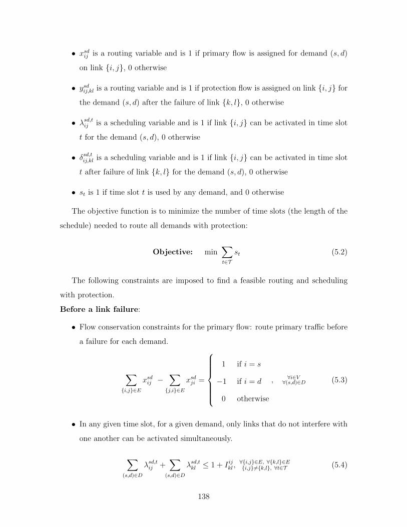
• xsdij is a routing variable and is 1 if primary flow is assigned for demand (s, d)

on link {i, j}, 0 otherwise

• ysdij,kl is a routing variable and is 1 if protection flow is assigned on link {i, j} for

the demand (s, d) after the failure of link {k, l}, 0 otherwise

• λsd,tij is a scheduling variable and is 1 if link {i, j} can be activated in time slot

t for the demand (s, d), 0 otherwise

• δsd,tij,kl is a scheduling variable and is 1 if link {i, j} can be activated in time slot

t after failure of link {k, l} for the demand (s, d), 0 otherwise

• st is 1 if time slot t is used by any demand, and 0 otherwise

The objective function is to minimize the number of time slots (the length of the

schedule) needed to route all demands with protection:

Objective: min∑t∈T

st (5.2)

The following constraints are imposed to find a feasible routing and scheduling

with protection.

Before a link failure:

• Flow conservation constraints for the primary flow: route primary traffic before

a failure for each demand.

∑{i,j}∈E


xsdji =

1 if i = s

−1 if i = d

0 otherwise

, ∀i∈V∀(s,d)∈D (5.3)

• In any given time slot, for a given demand, only links that do not interfere with

one another can be activated simultaneously.

∑(s,d)∈D

λsd,tij +∑

(s,d)∈D

λsd,tkl ≤ 1 + I ijkl ,∀{i,j}∈E, ∀{k,l}∈E{i,j}6={k,l}, ∀t∈T (5.4)

138

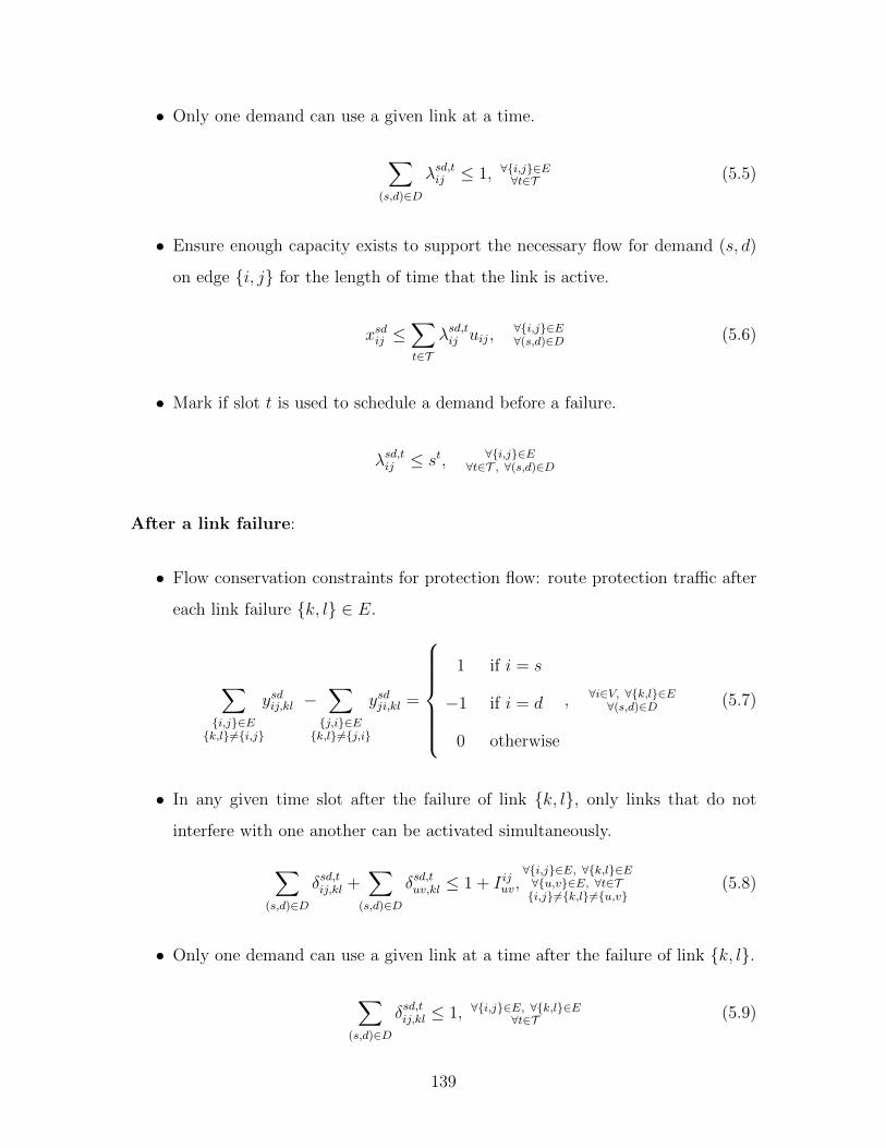
• Only one demand can use a given link at a time.

∑(s,d)∈D

λsd,tij ≤ 1, ∀{i,j}∈E∀t∈T (5.5)

• Ensure enough capacity exists to support the necessary flow for demand (s, d)

on edge {i, j} for the length of time that the link is active.

xsdij ≤∑t∈T

λsd,tij uij,∀{i,j}∈E∀(s,d)∈D (5.6)

• Mark if slot t is used to schedule a demand before a failure.

λsd,tij ≤ st, ∀{i,j}∈E∀t∈T , ∀(s,d)∈D

After a link failure:

• Flow conservation constraints for protection flow: route protection traffic after

each link failure {k, l} ∈ E.

∑{i,j}∈E{k,l}6={i,j}

ysdij,kl −∑{j,i}∈E{k,l}6={j,i}

ysdji,kl =

1 if i = s

−1 if i = d

0 otherwise

, ∀i∈V, ∀{k,l}∈E∀(s,d)∈D (5.7)

• In any given time slot after the failure of link {k, l}, only links that do not

interfere with one another can be activated simultaneously.

∑(s,d)∈D

δsd,tij,kl +∑

(s,d)∈D

δsd,tuv,kl ≤ 1 + I ijuv,∀{i,j}∈E, ∀{k,l}∈E∀{u,v}∈E, ∀t∈T{i,j}6={k,l}6={u,v}

(5.8)

• Only one demand can use a given link at a time after the failure of link {k, l}.

∑(s,d)∈D

δsd,tij,kl ≤ 1, ∀{i,j}∈E, ∀{k,l}∈E∀t∈T (5.9)

139

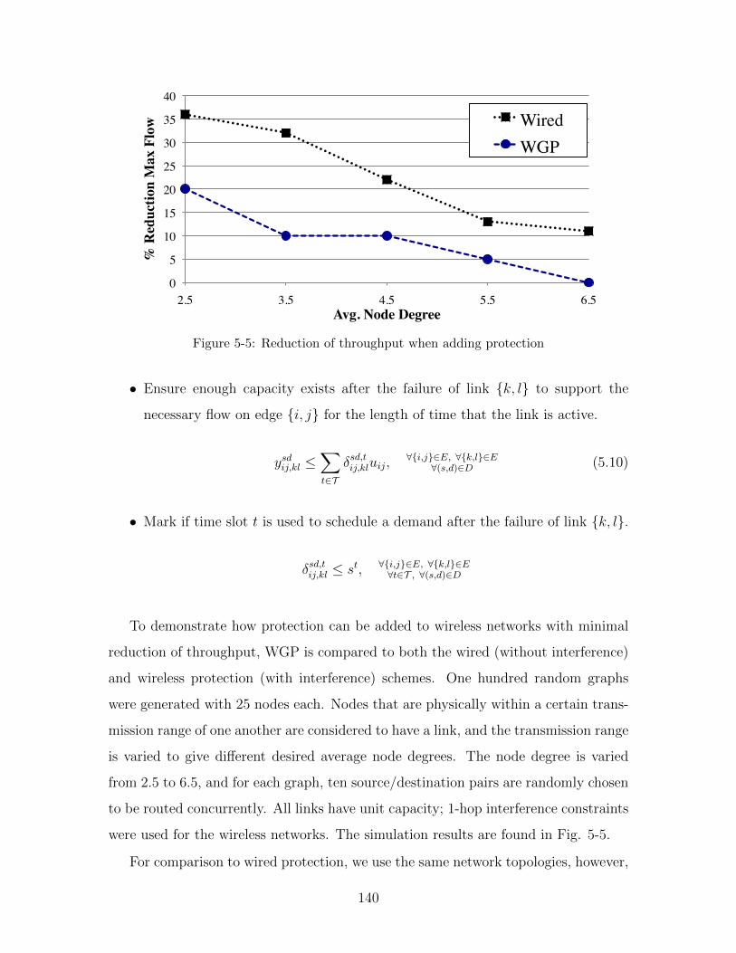
0

5

10

15

20

25

30

35

40

2.5 3.5 4.5 5.5 6.5

% R

educ

tion

Max

Flo

w

Avg. Node Degree

Wired WGP

Figure 5-5: Reduction of throughput when adding protection

• Ensure enough capacity exists after the failure of link {k, l} to support the

necessary flow on edge {i, j} for the length of time that the link is active.

ysdij,kl ≤∑t∈T

δsd,tij,kluij,∀{i,j}∈E, ∀{k,l}∈E

∀(s,d)∈D (5.10)

• Mark if time slot t is used to schedule a demand after the failure of link {k, l}.

δsd,tij,kl ≤ st, ∀{i,j}∈E, ∀{k,l}∈E∀t∈T , ∀(s,d)∈D

To demonstrate how protection can be added to wireless networks with minimal

reduction of throughput, WGP is compared to both the wired (without interference)

and wireless protection (with interference) schemes. One hundred random graphs

were generated with 25 nodes each. Nodes that are physically within a certain trans-

mission range of one another are considered to have a link, and the transmission range

is varied to give different desired average node degrees. The node degree is varied

from 2.5 to 6.5, and for each graph, ten source/destination pairs are randomly chosen

to be routed concurrently. All links have unit capacity; 1-hop interference constraints

were used for the wireless networks. The simulation results are found in Fig. 5-5.

For comparison to wired protection, we use the same network topologies, however,

140

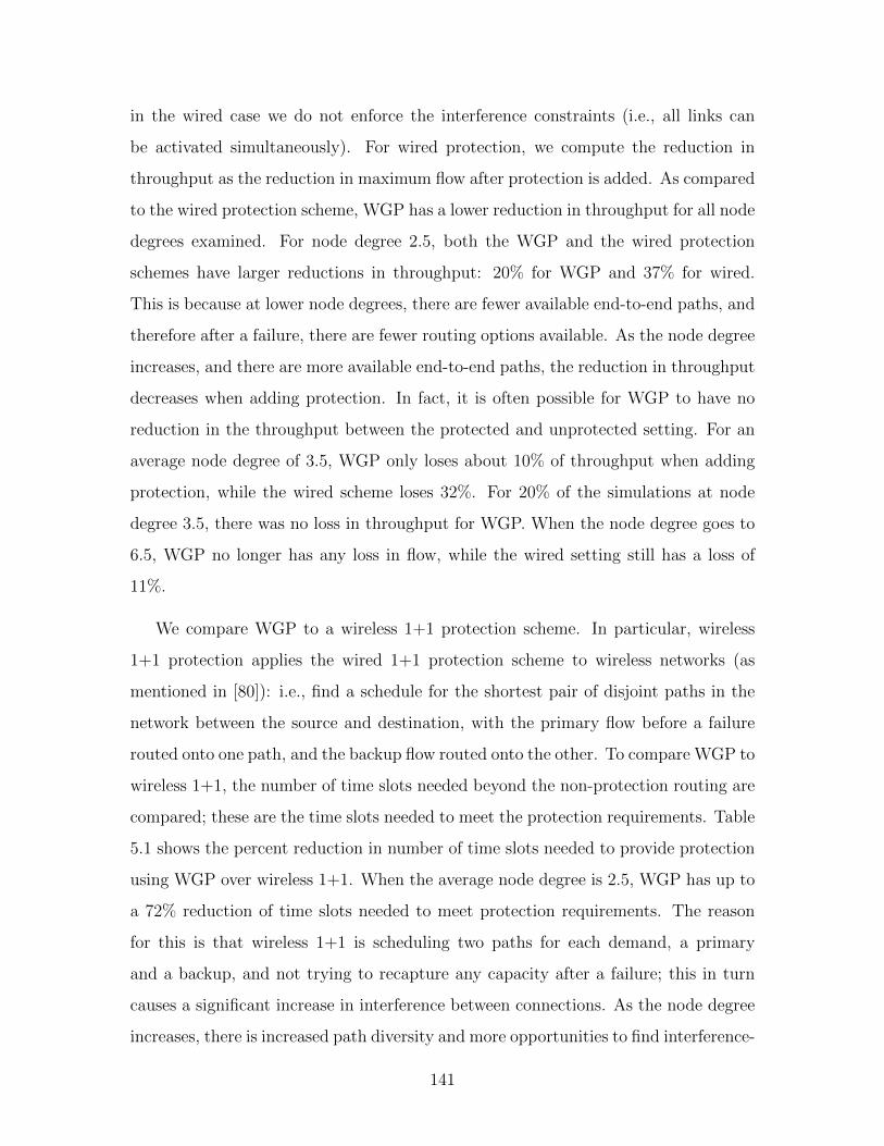
in the wired case we do not enforce the interference constraints (i.e., all links can

be activated simultaneously). For wired protection, we compute the reduction in

throughput as the reduction in maximum flow after protection is added. As compared

to the wired protection scheme, WGP has a lower reduction in throughput for all node

degrees examined. For node degree 2.5, both the WGP and the wired protection

schemes have larger reductions in throughput: 20% for WGP and 37% for wired.

This is because at lower node degrees, there are fewer available end-to-end paths, and

therefore after a failure, there are fewer routing options available. As the node degree

increases, and there are more available end-to-end paths, the reduction in throughput

decreases when adding protection. In fact, it is often possible for WGP to have no

reduction in the throughput between the protected and unprotected setting. For an

average node degree of 3.5, WGP only loses about 10% of throughput when adding

protection, while the wired scheme loses 32%. For 20% of the simulations at node

degree 3.5, there was no loss in throughput for WGP. When the node degree goes to

6.5, WGP no longer has any loss in flow, while the wired setting still has a loss of

11%.

We compare WGP to a wireless 1+1 protection scheme. In particular, wireless

1+1 protection applies the wired 1+1 protection scheme to wireless networks (as

mentioned in [80]): i.e., find a schedule for the shortest pair of disjoint paths in the

network between the source and destination, with the primary flow before a failure

routed onto one path, and the backup flow routed onto the other. To compare WGP to

wireless 1+1, the number of time slots needed beyond the non-protection routing are

compared; these are the time slots needed to meet the protection requirements. Table

5.1 shows the percent reduction in number of time slots needed to provide protection

using WGP over wireless 1+1. When the average node degree is 2.5, WGP has up to

a 72% reduction of time slots needed to meet protection requirements. The reason

for this is that wireless 1+1 is scheduling two paths for each demand, a primary

and a backup, and not trying to recapture any capacity after a failure; this in turn

causes a significant increase in interference between connections. As the node degree

increases, there is increased path diversity and more opportunities to find interference-

141

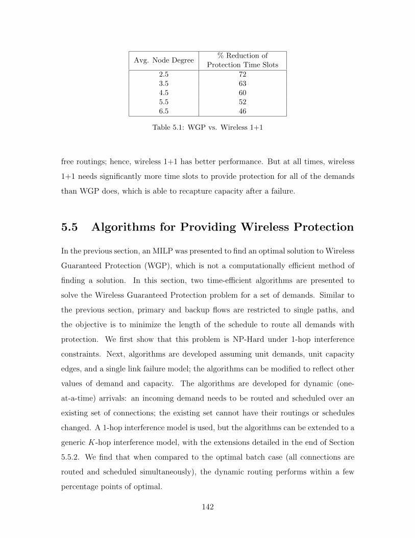
Avg. Node Degree% Reduction of

Protection Time Slots

2.5 723.5 634.5 605.5 526.5 46

Table 5.1: WGP vs. Wireless 1+1

free routings; hence, wireless 1+1 has better performance. But at all times, wireless

1+1 needs significantly more time slots to provide protection for all of the demands

than WGP does, which is able to recapture capacity after a failure.

5.5 Algorithms for Providing Wireless Protection

In the previous section, an MILP was presented to find an optimal solution to Wireless

Guaranteed Protection (WGP), which is not a computationally efficient method of

finding a solution. In this section, two time-efficient algorithms are presented to

solve the Wireless Guaranteed Protection problem for a set of demands. Similar to

the previous section, primary and backup flows are restricted to single paths, and

the objective is to minimize the length of the schedule to route all demands with

protection. We first show that this problem is NP-Hard under 1-hop interference

constraints. Next, algorithms are developed assuming unit demands, unit capacity

edges, and a single link failure model; the algorithms can be modified to reflect other

values of demand and capacity. The algorithms are developed for dynamic (one-

at-a-time) arrivals: an incoming demand needs to be routed and scheduled over an

existing set of connections; the existing set cannot have their routings or schedules

changed. A 1-hop interference model is used, but the algorithms can be extended to a

generic K-hop interference model, with the extensions detailed in the end of Section

5.5.2. We find that when compared to the optimal batch case (all connections are

routed and scheduled simultaneously), the dynamic routing performs within a few

percentage points of optimal.

142

First, in Section 5.5.1, we demonstrate WGP to be NP-Hard under 1-hop inter-

ference constraints when flows are restricted to a single path. Next, in Section 5.5.2,

an algorithm to find a shortest 1-hop interference-free path using a minimal num-

ber of time slots is presented. This serves as the building block for the next two

algorithms that are developed. In Section 5.5.3, an algorithm for finding a minimal

length schedule for WGP is presented, where a backup route and schedule is found

for each possible failure. This approach has drawbacks in that after any failure, a new

route is found; hence, a route and schedule for each failure event needs to be stored.

To overcome this, an algorithm is developed in Section 5.5.4 using disjoint paths

such that only two paths are needed: a primary and a backup. In Section 5.5.5, the

performance of the two algorithms are compared to the optimal MILP formulation.

5.5.1 Complexity Results under 1-hop Interference Constraints

Without protection, the routing and scheduling problem is NP-Hard under general

interference constraints [36]. But if flows for each demand are allowed to be split,

a polynomial timed algorithm is possible for 1-hop interference constraints [82]. We

demonstrate that when flows cannot be split, the routing and scheduling problem

becomes NP-Hard under 1-hop interference constraints.

Theorem 5.1. Finding the minimum length schedule to route a set of demands under

1-hop interference constraints when flow splitting is not allowed is NP-Hard.

We first consider the following necessary and sufficient condition for routing a set

node-disjoint1 pairs, (s1, d1), ..., (sN , dN), in only two time slots without flow splitting.

Lemma 5.6. Under 1-hop interference constraints, a set of demands that are node-

disjoint can be routed and scheduled using two time slots without flow splitting if and

only if there exists node-disjoint paths between each of the node pairs.

Proof. If there exists a node-disjoint path between every node pair in the set of de-

mands, then a schedule using two slots is possible. A proof can be accomplished by

1A node is a source or destination for at most one demand.

143

construction. Any individual path can be scheduled in two time slots by using alter-

nating time slots. If all paths are node-disjoint, then there exists no conflicts between

paths under 1-hop interference constraints. Therefore, all paths can be scheduled

using the same two-time slots.

For the other direction, assume otherwise: a two slot schedule is possible without

there being a node-disjoint path between every pair of nodes in the set of demands.

There exists a node v that has m ≥ 2 paths crossing it. There are m paths coming into

v and m paths out that need to be scheduled. Under 1-hop interference constraints,

this will require at least 2m time slots to produce an interference free schedule.

Using Lemma 5.6, Theorem 5.1 can be quickly demonstrated.

Proof of Theorem 5.1. We reduce the Disjoint Connecting Paths Problem (DCPP)

[37] to ours. DCPP asks the following question: given a graph G = (V,E) and a

collection of N node-disjoint pairs (s1, d1), ..., (sN , dN), does G contain N mutually

node-disjoint paths, one connecting si and di for each i, 1 ≤ i ≤ N? We can ask

an equivalent question for our routing and scheduling problem: can a set of N node-

disjoint pairs be routed and scheduled using the minimal number of time slots (two)

under 1-hop interference constraints without flow splitting? If yes, then by Lemma

5.6 that means we have found N mutually node-disjoint paths, one connecting si and

di for each i, 1 ≤ i ≤ N , which solves DCPP. An answer of no means a solution to

DCPP does not exist.

Next, we extend this complexity result to the case when protection is required.

Theorem 5.2. Finding the minimum length schedule to route a set of demands with

protection under 1-hop interference constraints without flow splitting is NP-Hard.

The proof can be found in Chapter Appendix Section 5.7.3.

5.5.2 Minimum Schedule for an Interference Free Path

We begin by developing an algorithm to find a shortest interference-free path using the

minimum number of time slots under the 1-hop interference model. This algorithm

144

will be a building block for the two protection algorithms that will be discussed in

the upcoming sections. We consider an incoming demand for a connection between

nodes s and d. Connections already exist in the network, with the set of T time slots

already in use. Based on how the current connections are routed and scheduled, a

set of edge interferences I can be constructed, where for every edge {i, j}, Iij ∈ I is

the set of time slots that cannot be used on that edge because either that time slot

is already used by {i, j}, or using that time slot on {i, j} will interfere with another

edge using it at that time. The set of edge interferences I can be constructed in

polynomial time, and will be given as an input to the algorithm.

First, we wish to determine the shortest interference free path without using any

additional time slots beyond the set T , and without rescheduling or rerouting existing

connections. Each edge {i, j} has a set of free time slots during which it can be used:

τij = T \ Iij. Let P be the set of edges used in a path. If each edge of a loop-free

path P has at least two free time slots, then that path can be scheduled without

interference using the existing time slot allocation T .

Lemma 5.7. For 1-hop interference, a loop-free path P can be scheduled without

interference if |τij| ≥ 2, ∀{i, j} ∈ P .

Proof. If |τij| ≥ 2, ∀{i, j} ∈ P , then each edge in P has an available time slot that

does not interfere with its adjacent set of edges. Since the path is loop-free, any two

edges that use the same time slot will never be less than one hop apart from one

another, and therefore never interfere with each other.

Using the result from Lemma 5.7, the following algorithm is constructed to find a

1-hop interference-free path using only the set of time slots T : remove all edges in G

that have |τij| ≤ 1, find the shortest path Psd between s and d, and assign time slots

to the edges in Psd such that it has an interference-free schedule.

An improvement can be made to the algorithm by attempting to maximize the

number of free time slots on any edge, so that future connections will be less likely

to require additional time slots to find an interference-free path. Currently, edges

that have many free time slots are not given any preference. If an edge has only the

145

minimal number of free time slots, it may be selected for use in a path. This may

hurt finding interference-free paths for future connections by limiting the number of

available time slots on an edge, thus necessitating new time slots. We assign a cost

for each edge to be equal to the number of time slots that that edge interferes with:

cij = |Iij|. With respect to these new edge costs, a minimum-cost interference-free

path is found. The more time slots an edge is in conflict with, the more expensive that

edge will be, and the less likely it will be used in a route. We refer to this algorithm

as int free path, which will return the edges and schedule of a path between s

and d.

To find an interference free path that tries to minimize future conflicts, and using

minimum additional time slots, we first find a minimum-cost interference free path

for the current set of time slots assigned in the network, T . If such a path does not

exist, increase the set of available time slots by 1, and repeat. We note that the set

of time slots will never increase by more than two since a feasible schedule can be

found for any path with two free time slots. We call this algorithm find path.

5.5.3 Minimum Length Schedule for Wireless Protection

In this section, an algorithm is developed that tries to find the minimum length

schedule for the Wireless Guaranteed Protection problem, with an approach that is

similar to the optimal solution found by the MILP in Section 5.4. The problem is

broken up into |E| + 1 subproblems. First, the minimum length schedule is found

to route the set of demands before a failure. Then, for each possible failure, the

minimum length schedule is found to route the set of demands on a failure graph

Gkl = (V,E \{k, l}), ∀{k, l} ∈ E (i.e., the graph that remains after the failure of edge

{k, l}). Each of the solutions to these subproblems represents the route and schedule

necessary to meet the protection requirements for the set of demands before and after

any link failure.

The maximum of any of these minimum length schedules will be the length of

the schedule needed to add protection to set of demands in a wireless network. The

algorithm is called minimum protect; it will return the set of paths and schedules

146

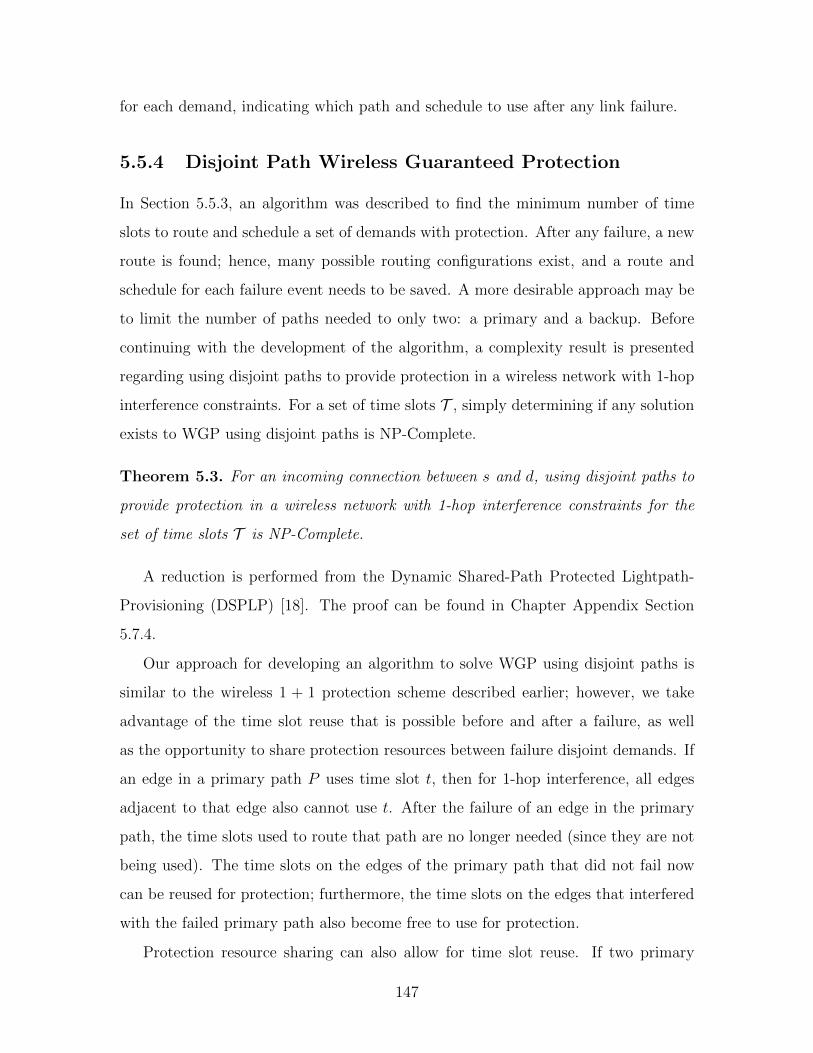
for each demand, indicating which path and schedule to use after any link failure.

5.5.4 Disjoint Path Wireless Guaranteed Protection

In Section 5.5.3, an algorithm was described to find the minimum number of time

slots to route and schedule a set of demands with protection. After any failure, a new

route is found; hence, many possible routing configurations exist, and a route and

schedule for each failure event needs to be saved. A more desirable approach may be

to limit the number of paths needed to only two: a primary and a backup. Before

continuing with the development of the algorithm, a complexity result is presented

regarding using disjoint paths to provide protection in a wireless network with 1-hop

interference constraints. For a set of time slots T , simply determining if any solution

exists to WGP using disjoint paths is NP-Complete.

Theorem 5.3. For an incoming connection between s and d, using disjoint paths to

provide protection in a wireless network with 1-hop interference constraints for the

set of time slots T is NP-Complete.

A reduction is performed from the Dynamic Shared-Path Protected Lightpath-

Provisioning (DSPLP) [18]. The proof can be found in Chapter Appendix Section

5.7.4.

Our approach for developing an algorithm to solve WGP using disjoint paths is

similar to the wireless 1 + 1 protection scheme described earlier; however, we take

advantage of the time slot reuse that is possible before and after a failure, as well

as the opportunity to share protection resources between failure disjoint demands. If

an edge in a primary path P uses time slot t, then for 1-hop interference, all edges

adjacent to that edge also cannot use t. After the failure of an edge in the primary

path, the time slots used to route that path are no longer needed (since they are not

being used). The time slots on the edges of the primary path that did not fail now

can be reused for protection; furthermore, the time slots on the edges that interfered

with the failed primary path also become free to use for protection.

Protection resource sharing can also allow for time slot reuse. If two primary

147

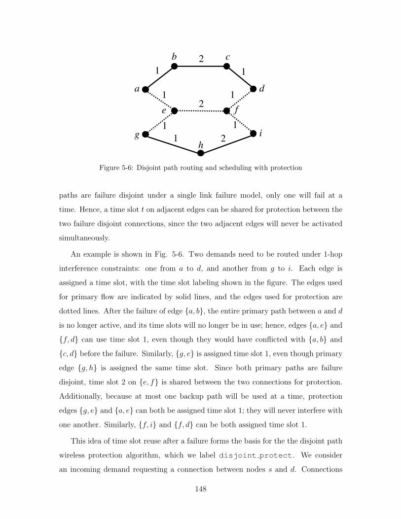
a

f

c

d

b

e

g i h

1 2

1

1 2

1

1 1 2

1

Figure 5-6: Disjoint path routing and scheduling with protection

paths are failure disjoint under a single link failure model, only one will fail at a

time. Hence, a time slot t on adjacent edges can be shared for protection between the

two failure disjoint connections, since the two adjacent edges will never be activated

simultaneously.

An example is shown in Fig. 5-6. Two demands need to be routed under 1-hop

interference constraints: one from a to d, and another from g to i. Each edge is

assigned a time slot, with the time slot labeling shown in the figure. The edges used

for primary flow are indicated by solid lines, and the edges used for protection are

dotted lines. After the failure of edge {a, b}, the entire primary path between a and d

is no longer active, and its time slots will no longer be in use; hence, edges {a, e} and

{f, d} can use time slot 1, even though they would have conflicted with {a, b} and

{c, d} before the failure. Similarly, {g, e} is assigned time slot 1, even though primary

edge {g, h} is assigned the same time slot. Since both primary paths are failure

disjoint, time slot 2 on {e, f} is shared between the two connections for protection.

Additionally, because at most one backup path will be used at a time, protection

edges {g, e} and {a, e} can both be assigned time slot 1; they will never interfere with

one another. Similarly, {f, i} and {f, d} can be both assigned time slot 1.

This idea of time slot reuse after a failure forms the basis for the the disjoint path

wireless protection algorithm, which we label disjoint protect. We consider

an incoming demand requesting a connection between nodes s and d. Connections

148

already exist in the network, with the set of T time slots already in use. A interference-

free primary path between s and d, Psd, is found using find path. Once a primary

path fails, none of the time slots needed for that path, or on the edges that interfered

with that path, are needed, and they become available to be used for protection. Next,

a backup path Bsd is found that is disjoint to Psd, and does not interfere with any of

the other connections that did not fail. Additionally, the backup path Bsd will not

interfere with the protection routings for the different existing demands that would

fail if an edge in Psd fails (i.e., Bsd will not interfere with the protection paths for

demands whose primary paths are not disjoint with Psd). The algorithm is detailed

in Algorithm 3.

Algorithm 3(Psd,I, T ) = disjoint protect(G,I, T , s, d)

Find route and schedule before a failure:(Psd, T , I′) = find path(G, I, T , s, d)

Construct new network without the edges in path Psd:GF = (V,E \ Psd)

Once an edge for that demand fails, none of the slots needed to support it are usedand become available. Construct a failure interference set using the interference setfor the primary routes before that demand was routed, and the failure interferencesets for each edge {k, l} in Psd

IF = (∪{k,l}∈PsdIkl) ∪ I

Find a disjoint path, and schedule it:(P F

sd, T , I′′) = find path(GF , IF , T , s, d)Update interference sets:

Before a failure: I = I′

After each primary path failure: Ikl = I′′, ∀{k, l} ∈ PsdI = Set of I and all Ikl

Psd = Set of Psd and all P klsd

Return (Psd,I, T )

5.5.5 WGP Algorithm Simulations

The algorithms minimum protect and disjoint protect are compared to the

optimal solution found by the MILP in Section 5.4. A similar simulation setup is used

as that in Section 5.4. One hundred random graphs were generated with 25 nodes

each. The node degree is varied from 2.5 to 6.5, and for each random graph, ten

149

5

6

7

8

9

10

11

12

13

2.5 3.5 4.5 5.5 6.5

Avg.

Min

Len

gth

Sche

dule

Avg. Node Degree

Disjoint Minimum MILP

Figure 5-7: Avg. time slots needed for WGP

source/destination pairs are randomly chosen to be routed concurrently, each with a

unit demand. All links have unit capacity, and 1-hop interference constraints were

used. The algorithms route and schedule demands one-at-a-time, while the MILP

optimizes the route and schedule for all demands together (in batch). To compare

the two, the algorithms randomly order the set of demands, and then solves for each

demand one-at-a-time. The simulation results are found in Fig. 5-7.

Similar to the previous simulation, as node degree increased, the average mini-

mum length schedule decreased. This is because of the increased diversity in possible

number of end-to-end path, which leads to a greater opportunity of finding interfer-

ence free paths. On average, minimum protect needed only 4.5% more time slots

to meet all requirements than the optimal MILP needed, and disjoint protect

needed 10.1% more time slots than the MILP.

5.6 Conclusion

In this chapter, the problem of guaranteed protection in a multi-hop wireless network

is introduced. Because of link interference, resources that were unavailable prior to

a failure can be used for protection after the failure. In fact, protection can often

150

be provided using no additional resources. For the case of a single demand with 1-

hop interference constraints, properties of an optimal solution are presented, and a

time-efficient algorithm is developed that solves the problem of wireless routing and

scheduling with and without protection, guaranteeing a maximum throughput that

is within 1.5 of optimal. For general interference constraints and multiple concurrent

demands, an optimal solution is developed for the protection problem via a mixed

integer linear program. When compared to using traditional wired protection schemes

on a wireless network, our Wireless Guaranteed Protection (WGP) scheme uses as

much as 72% less protection resources to achieve the same level of resiliency. Two low-

complexity algorithms to solve WGP are developed, and on average, these algorithms

perform close to the optimal solution. A future direction for our work is to adapt the

schemes developed in this chapter to a distributed setting.


5.7.1 MILP for WGP with Different Throughputs

Some demand between nodes s and d has its own throughput requirement f sd. The

objective of the MILP is to minimize the number of times slots needed to schedule

every demand. Since each demand has a throughput requirement, finding a minimum

length schedule will be with respect to keeping the ratio of the different demands’

throughputs constant. We assume f sd is integer ∀(s, d) ∈ (V, V ). If necessary, the

demands and link capacities can be scaled by the smallest integer that makes all

demand values integer (hence, f sd is assumed to be at the very least rational, ∀(s, d) ∈

(V, V )).



• D is the set of flow requirements

• f sd is the flow required between nodes (s, d); f sd ∈ Z

151

• uij is the capacity of link {i, j}

• I is the interference matrix, where Iklij ∈ I is 1 if links {i, j} and {k, l} can be

activated simultaneously, 0 otherwise

• T is the set of time slots in the system, T ⊂ Z+

The MILP solves for the following variables:

• xsdij is a routing variable and is 1 if primary flow is assigned for demand (s, d)

on link {i, j}, 0 otherwise

• ysdij,kl is a routing variable and is 1 if protection flow is assigned on link {i, j} for

the demand (s, d) after the failure of link {k, l}, 0 otherwise

• λsd,tij is a scheduling variable and is 1 if link {i, j} can be activated in time slot

t for the demand (s, d), 0 otherwise

• δsd,tij,kl is a scheduling variable and is 1 if link {i, j} can be activated in time slot

t after failure of link {k, l} for the demand (s, d), 0 otherwise

• st is 1 if time slot t is used by any demand, and 0 otherwise

The objective function is to minimize the number of time slots (the length of the

schedule) needed to route all demands with protection:

Objective: min∑t∈T

st (5.11)

The following constraints are imposed to find a feasible routing and scheduling

with protection.

Before a link failure:

• Flow conservation constraints for the primary flow: route primary traffic before

a failure for each demand.

152

∑{i,j}∈E


xsdji =

1 if i = s

−1 if i = d

0 otherwise

, ∀i∈V∀(s,d)∈D (5.12)

• In any given time slot, for a given demand, only links that do not interfere with

one another can be activated simultaneously.

∑(s,d)∈D

λsd,tij +∑

(s,d)∈D

λsd,tkl ≤ 1 + I ijkl ,∀{i,j}∈E, ∀{k,l}∈E{i,j}6={k,l}, ∀t∈T (5.13)

• Only one demand can use a given link at a time.

∑(s,d)∈D

λsd,tij ≤ 1, ∀{i,j}∈E∀t∈T (5.14)

• Ensure enough capacity exists to support the necessary flow f sd for demand

(s, d) on edge {i, j} for the length of time that the link is active.

f sdxsdij ≤∑t∈T

λsd,tij uij,∀{i,j}∈E∀(s,d)∈D (5.15)

• Mark if slot t is used to schedule a demand before a failure.

λsd,tij ≤ st, ∀{i,j}∈E∀t∈T , ∀(s,d)∈D

After a link failure:

• Flow conservation constraints for protection flow: route protection traffic after

each link failure {k, l} ∈ E.

∑{i,j}∈E{k,l}6={i,j}

ysdij,kl −∑{j,i}∈E{k,l}6={j,i}

ysdji,kl =

1 if i = s

−1 if i = d

0 otherwise

, ∀i∈V, ∀{k,l}∈E∀(s,d)∈D (5.16)

153

• In any given time slot after the failure of link {k, l}, only links that do not

interfere with one another can be activated simultaneously.

∑(s,d)∈D

δsd,tij,kl +∑

(s,d)∈D

δsd,tuv,kl ≤ 1 + I ijuv,∀{i,j}∈E, ∀{k,l}∈E∀{u,v}∈E, ∀t∈T{i,j}6={k,l}6={u,v}

(5.17)

• Only one demand can use a given link at a time after the failure of link {k, l}.

∑(s,d)∈D

δsd,tij,kl ≤ 1, ∀{i,j}∈E, ∀{k,l}∈E∀t∈T (5.18)

• Ensure enough capacity exists after the failure of link {k, l} to support the

necessary flow f sd on edge {i, j} for the length of time that the link is active.

f sdysdij,kl ≤∑t∈T

δsd,tij,kluij,∀{i,j}∈E, ∀{k,l}∈E

∀(s,d)∈D (5.19)

• Mark if time slot t is used to schedule a demand after the failure of link {k, l}.

δsd,tij,kl ≤ st, ∀{i,j}∈E, ∀{k,l}∈E∀t∈T , ∀(s,d)∈D

5.7.2 Schedules for Higher Throughput on Node-Disjoint Paths

with an Odd Number of Edges

In Section 5.3.1, for a pair of node-disjoint paths whose total number of edges is odd,

a schedule using three time slots was used to achieve a flow of 23

between the source

and the destination. Each link is assigned one of three time slots, and since each

link is active for only 13

of the time, each path supports a flow of 13, and the total

end-to-end flow is 23. An example is shown on the five edge network in Figure 5-8a.

By using additional time slots, it is in fact possible to increase the end-to-end

throughput. For the same five edge network, a maximum flow of 56

is possible using

six time slots. A schedule that achieves this flow is shown in Figure 5-8b. On the

shorter path, three time slots are assigned to each link. Since there are a total of six

154

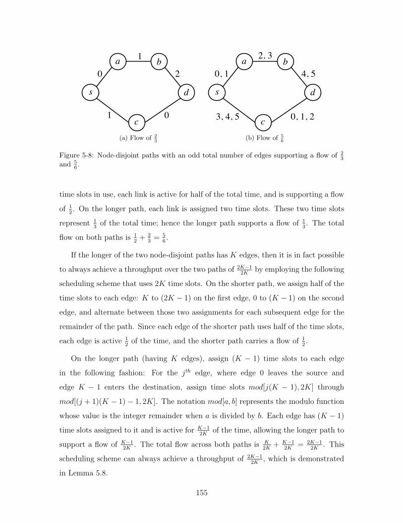
s d

a

c

0

1 0

1 b 2

(a) Flow of 23

s d

a

c

0, 1

3, 4, 5 0, 1, 2

2, 3 b 4, 5

(b) Flow of 56

Figure 5-8: Node-disjoint paths with an odd total number of edges supporting a flow of 23

and 56 .

time slots in use, each link is active for half of the total time, and is supporting a flow

of 12. On the longer path, each link is assigned two time slots. These two time slots

represent 13

of the total time; hence the longer path supports a flow of 13. The total

flow on both paths is 12

+ 23

= 56.

If the longer of the two node-disjoint paths has K edges, then it is in fact possible

to always achieve a throughput over the two paths of 2K−12K

by employing the following

scheduling scheme that uses 2K time slots. On the shorter path, we assign half of the

time slots to each edge: K to (2K − 1) on the first edge, 0 to (K − 1) on the second

edge, and alternate between those two assignments for each subsequent edge for the

remainder of the path. Since each edge of the shorter path uses half of the time slots,

each edge is active 12

of the time, and the shorter path carries a flow of 12.

On the longer path (having K edges), assign (K − 1) time slots to each edge

in the following fashion: For the jth edge, where edge 0 leaves the source and

edge K − 1 enters the destination, assign time slots mod[j(K − 1), 2K] through

mod[(j + 1)(K − 1)− 1, 2K]. The notation mod[a, b] represents the modulo function

whose value is the integer remainder when a is divided by b. Each edge has (K − 1)

time slots assigned to it and is active for K−12K

of the time, allowing the longer path to

support a flow of K−12K

. The total flow across both paths is K2K

+ K−12K

= 2K−12K

. This

scheduling scheme can always achieve a throughput of 2K−12K

, which is demonstrated

in Lemma 5.8.

155

Two examples are shown in Figure 5-9. In the first network, shown in Figure

5-9a, the longer path has five edges (K = 5), and the shorter has four. Ten time slots

are used in total, with the shorter path supporting a flow of 12, and the longer path

supporting a flow of 45, resulting in an end-to-end flow of 9

10. It is straightforward to

see that if the shorter path had two edges instead of four, the same throughput would

have been achievable using the same ten time slots. In the second network, shown in

Figure 5-9b, the longer path has four edges (K = 4), and the shorter has three; eight

time slots are used. The shorter path supports a flow of 12, the longer path supports

a flow of 38, and the total end-to-end flow is 7

8.

s d 0,1,2,3,4

0,1,2,3

5,6,7,8,9

4,5,6,7 8,9,0,1 2,3,4,5

6,7,8,9

5,6,7,8,9 0,1,2,3,4

(a) K = 5, and a flow of 910

s d

0,1,2,3 4,5,6,7 4,5,6,7

0,1,2

2,3,4 5,6,7

0,1,2

(b) K = 4, and a flow of 78

Figure 5-9: Node-disjoint paths with an odd number of edges supporting flows of 2K−12K

Lemma 5.8. For a pair of node-disjoint paths with an odd number of edges, where

the longer path has K edges, a schedule exists that achieves a throughput of 2K−12K

over

the two paths.

Proof. We demonstrate the scheduling scheme presented in this section always achieves

the desired rate of 2K−12K

. We consider two cases: K is odd, and K is even.

156

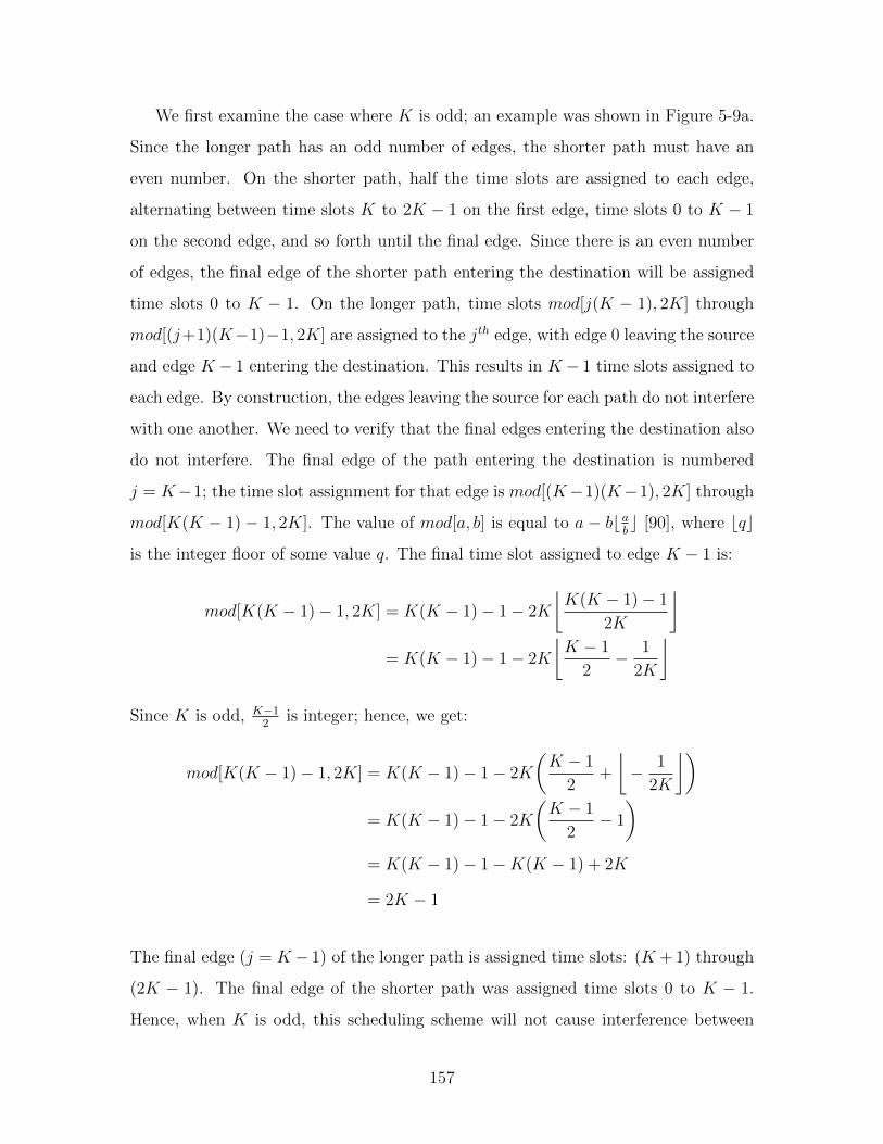
We first examine the case where K is odd; an example was shown in Figure 5-9a.

Since the longer path has an odd number of edges, the shorter path must have an

even number. On the shorter path, half the time slots are assigned to each edge,

alternating between time slots K to 2K − 1 on the first edge, time slots 0 to K − 1

on the second edge, and so forth until the final edge. Since there is an even number

of edges, the final edge of the shorter path entering the destination will be assigned

time slots 0 to K − 1. On the longer path, time slots mod[j(K − 1), 2K] through

mod[(j+1)(K−1)−1, 2K] are assigned to the jth edge, with edge 0 leaving the source

and edge K − 1 entering the destination. This results in K − 1 time slots assigned to

each edge. By construction, the edges leaving the source for each path do not interfere

with one another. We need to verify that the final edges entering the destination also

do not interfere. The final edge of the path entering the destination is numbered

j = K−1; the time slot assignment for that edge is mod[(K−1)(K−1), 2K] through

mod[K(K − 1) − 1, 2K]. The value of mod[a, b] is equal to a − bbabc [90], where bqc

is the integer floor of some value q. The final time slot assigned to edge K − 1 is:

mod[K(K − 1)− 1, 2K] = K(K − 1)− 1− 2K

⌊K(K − 1)− 1

2K

⌋= K(K − 1)− 1− 2K

⌊K − 1

2− 1

2K

⌋

Since K is odd, K−12

is integer; hence, we get:

mod[K(K − 1)− 1, 2K] = K(K − 1)− 1− 2K

(K − 1

2+

⌊− 1

2K

⌋)= K(K − 1)− 1− 2K

(K − 1

2− 1

)= K(K − 1)− 1−K(K − 1) + 2K

= 2K − 1

The final edge (j = K − 1) of the longer path is assigned time slots: (K + 1) through

(2K − 1). The final edge of the shorter path was assigned time slots 0 to K − 1.

Hence, when K is odd, this scheduling scheme will not cause interference between

157

adjacent edges, and will achieve an end-to-end flow of 2K−12K

.

We next demonstrate a similar result for when K is even; an example network

was shown in Figure 5-9b. The longer path has an even number of edges, and the

shorter path has an odd number. Again, on the shorter path, half the time slots

are assigned to each edge, alternating between time slots K to 2K − 1 on the first

edge, time slots 0 to K − 1 on the second edge, and so forth until the final edge.

Since there is an odd number of edges, the final edge of the shorter path entering

the destination will be assigned time slots K to 2K − 1. We now consider the final

edge entering the destination of the longer path, which will be assigned time slots

mod[(K−1)(K−1), 2K] through mod[K(K−1)−1, 2K]. The final time slot for this

edge will have the value mod[K(K − 1)− 1, 2K] = K(K − 1)− 1− 2KbK−12− 1

2Kc.

Since K is even, K−12

is not integer, but K2

is; hence, we get:

mod[K(K − 1)− 1, 2K] = K(K − 1)− 1− 2K

⌊K − 1

2− 1

2K

⌋= K(K − 1)− 1− 2K

(K

2+

⌊− 1

2− 1

2K

⌋)= K(K − 1)− 1− 2K

(K

2− 1

)= K2 −K − 1−K2 + 2K

= K − 1

The final edge of the longer path is assigned time slots 1 through (K − 1). The final

edge of the shorter path was assigned time slots K to 2K − 1. Therefore, when K

is even, this scheduling scheme will not cause interference between adjacent edges at

the destination, and will achieve an end-to-end flow of 2K−12K

.

Using the scheme described above, the minimum throughput that can be guaran-

teed on a pair of node-disjoint paths with an odd number of edges is 56, which is greater

than the 23

flow described in Section 5.3.1. The minimum guaranteed throughput of

56

is independent of K.

Lemma 5.9. For a pair of node-disjoint paths, a schedule can always be found that

158

guarantees a flow of at least 56

from the source to the destination.

Proof. We consider only the case when the source and destination are more than one

hop apart; otherwise, only one edge needs to be activated between the two nodes,

carrying the maximum flow of 1 without the use of node disjoint paths.

When there are an even number of edges over the two node-disjoint paths, then

the maximum flow of 1 can be achieved using two time slots, as was shown in Lemma

5.3.

When there are an odd number of edges over the two node-disjoint paths, where

the longer path has K edges, then a flow of 2K−12K

can always be achieved, which was

demonstrated in Lemma 5.8. We now show that the minimum K is 3, hence the

minimum flow is 56. Since the source and destination are more than one hop apart,

the minimum number of edges over both paths is 4. With 4 total edges, the two paths

have an even number of edges, and a maximum flow of 1 is achievable using two time

slots. The next smallest number of edges for both paths is 5. Since the source and

destination cannot be one hop apart, this means the longer path has 3 edges, and the

shorter has 2. Hence, the smallest value of K possible is 3, which gives an achievable

throughput of 2K−12K

= 56. Any value of K that is greater than 3 will result in a higher

achievable throughput.

If only a pair of node-disjoint paths exist with an odd number of edges between the

source and destination, a flow of 2K−12K

can found using 2K time slots. But this does

preclude the possibility of higher feasible throughputs existing that use additional

edges. Consider the example in Figure 5-10.

The pair of node-disjoint paths between nodes s and d are shown using the solid

edges, and additional edges that connect with one of the node-disjoint paths are

shown using the dotted edges. In this network, all possible pairs node-disjoint paths

have an odd number edges. The longer path has 4 edges; if we scheduled according

the scheme described earlier, a flow of 78

can be achieved between s and d. But by

using the dotted edges, in addition to the solid edges, a schedule can be found that

achieves the maximum flow of 1, as shown in Figure 5-10. This shows that the flow

159

s d

0,1,2,3

6,7

4,5,6,7 0,1,2,3

4,5,6,7

4,5 6,7

4,5

0,1,2,3

Figure 5-10: Node-disjoint paths with additional edges supporting a flow of 1

2K−12K

is strictly a lower bound on the maximum flow that can be found when only

a pair of node-disjoint paths exist that have an odd number of edges. We do not

currently consider the problem of determining whether or not a maximum flow of 1

exists in this case, and we leave it as future work.

5.7.3 Proof for Theorem 5.2

Theorem 5.2: Finding the minimum length schedule to route a set of demands with

protection under 1-hop interference constraints without flow splitting is NP-Hard.

Proof. We prove the protection version of the problem to be NP-hard by reducing the

non-protection version to it. We begin by taking a graph G = (V,E) and transforming

it to some other graph G′ = (V ′, E ′). Graph G′ will be constructed such that any

feasible solution in G using two time slots for node-disjoint paths for a set of node-

disjoint demands (i.e., a solution for the non-protection problem in G) will have an

immediate solution that includes protection using two time slots for the same set of

node-disjoint demands.

Consider an edge {i, j} of some path between s and d in G, which is node-disjoint

from any other path and is scheduled to use time slot 1. Three edges, {i, k}, {k, l},

and {l, j}, can be added to protect {i, j} without needing any additional time slots,

with time slot assignments as shown in Fig. 5-11. Edge {i, k} and {l, j} are assigned

time slot 1, and since they will only be activated after the failure of edge {i, j},

160

they do not conflict with the time slot assignment for {i, j}. Furthermore, the edge

on the path in G directly preceding and directly following edge {i, j} will be time

slot 2 (because the schedule only consisted of two time slots); so, after {i, j} fails,

the protection routing of {i, k}, {k, l}, and {l, j} will not interfere with the existing

scheduled edges of the path. Additionally, since we are currently considering a feasible

solution of node-disjoint paths for the set of node-disjoint demands, no node will have

more than a single path crossing it, so the protection path of {i, k}, {k, l}, and {l, j}

will not interfere with any other demands.

i j

k l

1

2 1 1 i j 1

Figure 5-11: Edge transformation for NP-hardness proof

To begin, it is clear that any solution for a non-protection routing in two time

slots for the set of node-disjoint demands in G will immediately give a protection

routing and schedule using two time slots in G′ for the same set of demands. We

now consider the other direction: for a set of node-disjoint demands, does a solution

that uses two time slots for the protection problem on G′ give a solution for the same

set of demands using two time slots for the non-protection problem in G? If the

protection problem returns a solution for a routing and scheduling using two slots,

then that means that before any failure, and after any failure, the set of node-disjoint

demands can be routed in two time slots. So, if a routing and schedule is found, then

we take the route and schedule from before a failure (which is in two time slots), and

transfer any flow that may have been routed onto {i, k}, {k, l}, and {l, j} to edge

{i, j}, with {i, j} having the same time slot assignment as {i, k}. Because of how our

transformation was performed, this will always yield a feasible solution for the set of

node-disjoint demands in G. In general, it is not necessarily the case that no solution

to the protection problem indicates no solution to the non-protection problem. But

for our particular graph transformation, this is the case; we know that if a two time

slot solution exists in G, then a protection routing must exist that uses two time slots.

161

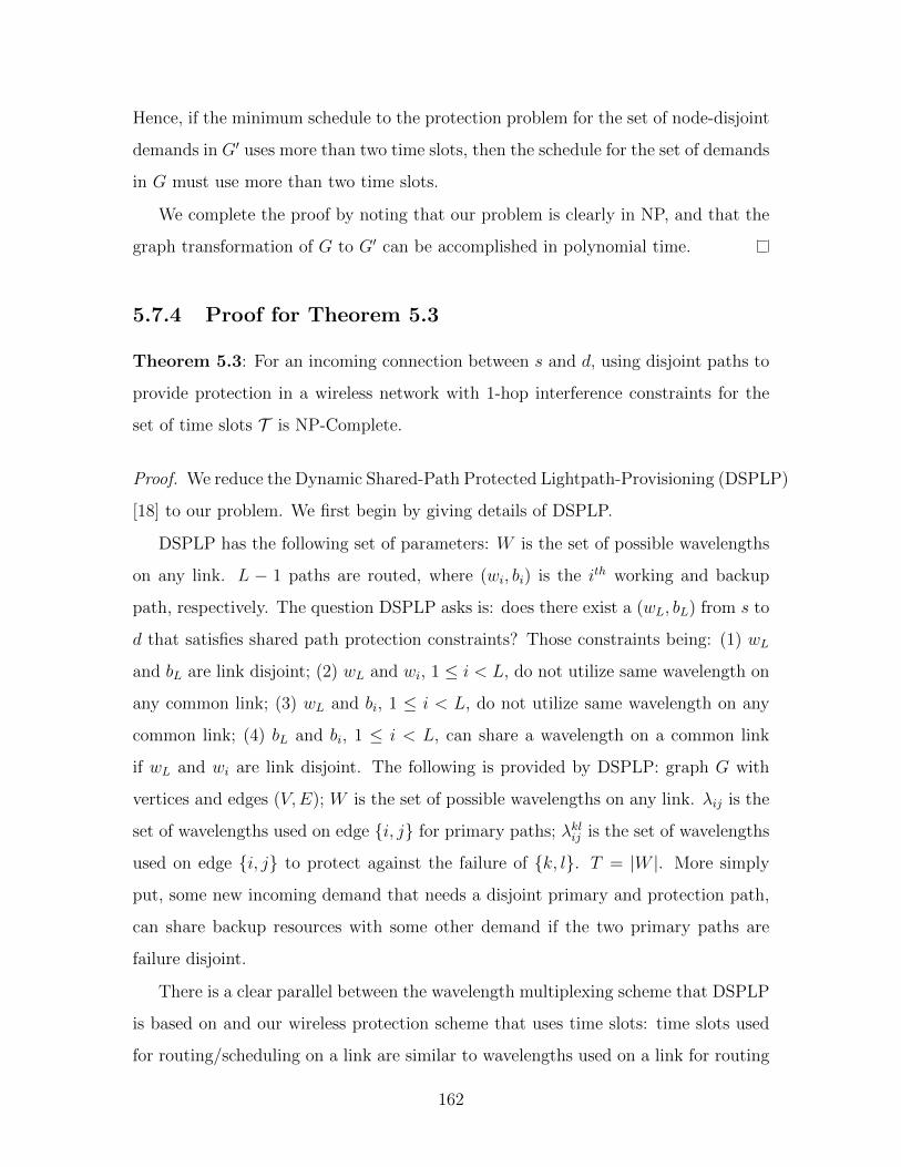
Hence, if the minimum schedule to the protection problem for the set of node-disjoint

demands in G′ uses more than two time slots, then the schedule for the set of demands

in G must use more than two time slots.

We complete the proof by noting that our problem is clearly in NP, and that the

graph transformation of G to G′ can be accomplished in polynomial time.

5.7.4 Proof for Theorem 5.3

Theorem 5.3: For an incoming connection between s and d, using disjoint paths to

provide protection in a wireless network with 1-hop interference constraints for the

set of time slots T is NP-Complete.

Proof. We reduce the Dynamic Shared-Path Protected Lightpath-Provisioning (DSPLP)

[18] to our problem. We first begin by giving details of DSPLP.

DSPLP has the following set of parameters: W is the set of possible wavelengths

on any link. L − 1 paths are routed, where (wi, bi) is the ith working and backup

path, respectively. The question DSPLP asks is: does there exist a (wL, bL) from s to

d that satisfies shared path protection constraints? Those constraints being: (1) wL

and bL are link disjoint; (2) wL and wi, 1 ≤ i < L, do not utilize same wavelength on

any common link; (3) wL and bi, 1 ≤ i < L, do not utilize same wavelength on any

common link; (4) bL and bi, 1 ≤ i < L, can share a wavelength on a common link

if wL and wi are link disjoint. The following is provided by DSPLP: graph G with

vertices and edges (V,E); W is the set of possible wavelengths on any link. λij is the

set of wavelengths used on edge {i, j} for primary paths; λklij is the set of wavelengths

used on edge {i, j} to protect against the failure of {k, l}. T = |W |. More simply

put, some new incoming demand that needs a disjoint primary and protection path,

can share backup resources with some other demand if the two primary paths are

failure disjoint.

There is a clear parallel between the wavelength multiplexing scheme that DSPLP

is based on and our wireless protection scheme that uses time slots: time slots used

for routing/scheduling on a link are similar to wavelengths used on a link for routing

162

and protection. In [18], NP-Completeness is shown for a network with T = 1; hence,

it is sufficient for us to demonstrate that if our problem can solve an instance of

DSPLP with only one wavelength, our problem is also NP-Complete.

If wavelengths are considered as timeslots, they will interfere with one another.

Clearly more than one time slot must exist in order to find a feasible routing and

schedule in a wireless network with 1-hop inference constraints. So, we “extend”

a “new” link from each node, and we increase T (the number of time slots in the

wireless network) such that there exists sufficient time slots to change existing paths

that use one wavelength in the original network into interference free schedules using

the “new” edges in GW . It is easy to see that the number of new time slots that

need to be added will be the maximum node degree of the network. An example is

shown in Fig. 5-12. The node degree is 4, and each edge has a path routed on it

using the existing wavelength. We extend “new” edges out of the node, and increase

the number of time slots to any value above 5. Now an interference free schedule can

be assigned to allow the edges that used wavelength 1 (now time slot 1) to continue

routing those paths using time slot 1.

1

1 1

1 1 1

(a) Node in DSPLP network

1

1 1

1 2 3

5 4

(b) Node with “new” edges

Figure 5-12: Time slot assignment for extended “new” edges

We modify the network G to GW in the following manner. We “extend” a “new”

link from each node, and increase TW (the number of time slots in the wireless

network) by some “large enough” value, such that the “new” edges in GW will never

interfere with one another, or with existing demands using wavelenth/time slot 1.

“Old” links in GW that used wavelength 1 to support a lightpath in G will have no

163

available time slots in GW . Since the primary links using wavelength 1 in G will no

have no free time slots in GW , every future incoming demand in GW will be edge-

disjoint from the existing primary demand that use wavelength/time slot 1, and hence

can share backup capacity with existing demands. All links in G that use wavelength

1 for protection will have only one free time slot (time slot 1) available for use in GW ,

and only as the backup path for a future demand in GW . All other “old” links in GW

will have only one time slot available, time slot 1, available for use for the primary or

protection path.

Consider some new incoming demand in GW that needs to be routed and sched-

uled with a disjoint primary and protection path. The way the network GW was

constructed will ensure that if a solution exists for the new demand, then a solution

exists for DSPLP in G. The new demand in GW will only be able to use time slot 1

on the ”old” links, which is wavelength 1. Any solution for wireless protection using

disjoint paths in GW can be converted to a solution for DSPLP in G by removing

the “new” edges. If no solution exists for wireless protection using disjoint paths in

GW , then it is clear that no solution exists for DSPLP in G. It is also clear that any

solution for DSPLP in G will solve wireless protection using disjoint paths in GW

(with the trivial addition of the “new” edges).

To complete the proof, we note that our problem is clearly in NP.

164

Chapter 6

Conclusion and Future Directions

In this thesis, we investigated providing network protection with a variety of ser-

vice guarantees that offer significant resource savings over traditional full protection

schemes. Because of the high cost of full protection, many network operators pro-

vide no protection whatsoever. In addition, traditional full protection typically offer

no guarantees on recovery time, which is becoming increasingly important with the

widespread use of real-time applications that cannot tolerate long disruptions. Fur-

thermore, network protection has not been adequately examined in wireless networks

because of the scarcity of resources available for backup and the complexity of allo-

cating these resources. By examining various service guarantees, we allow operators

to offer resource-efficient protection that fit the particular needs of their network.

In Chapter 2, we developed a network protection scheme called Partial Protection

that guarantees a quantifiable minimum grade of service upon a failure within the

network. In Chapter 3, we built upon the partial protection scheme developed in

Chapter 2 by adding the additional constraint of only allowing flow to drop to its

reduced service level for at most a certain probability after a network failure. In

Chapter 4, we switch focus from examining guaranteed partial flows after a failure

to considering the problem of providing network protection that guarantees the max-

imum amount of time that flow can be interrupted after a failure. In Chapter 5,

we move from the wired setting towards examining protection in wireless networks;

in particular, we investigate the problem of providing resource-efficient guaranteed

165

protection against failures in wireless networks subject to interference constraints.

We believe that the work on protection with various service guarantees is just

beginning. As communications continues to evolve, differing types of protection will

be necessary to fit the particular needs of future networks and services. One future

direction is to continue adapting the models and algorithms developed in this thesis.

One example is distributing these algorithms across the network such that there is

no need for a central planner. Another example is to study protocol design that will

allow the service guaranteed protection frameworks developed within this thesis to

be easily adapted into already existing networks. This work considered providing

protection for already existing networks. Another approach that can be taken is from

the network planning perspective: How can networks be designed such that they are

most conducive for protection with respect to the different service guarantees? This

question is particularly important for wireless networks that have limited resources

available for protection.

As data networks continue to rapidly change, there will never be a lack of future

directions for service guaranteed protection. Twenty years ago, the concept of “ser-

vices” that may have differing needs was not even considered; ten years ago, wireless,

cloud, and real-time services were too new to begin thinking of offering customized

protection; in ten years from now, new services will exist that we cannot predict

today, and they too will need protection to meet their particular needs. This thesis

offers a starting point on how to meet the current and future challenges of service

guaranteed protection.

166

Bibliography

[1] D. Xu, Y. Chen, Y. Xiong, C. Qiao, and X. He, “On finding disjoint paths insingle and dual link cost networks,” in INFOCOM 2004, vol. 1. IEEE, 2004.

[2] B. Mukherjee, “WDM Optical Communication Networks: Progress and chal-lenges,” IEEE Journal on Selected Areas in Communications, vol. 18, no. 10, pp.1810–1824, 2000.

[3] A. Saleh and J. Simmons, “Evolution Toward the Next-Generation Core OpticalNetwork,” Journal of Lightwave Technology, vol. 24, no. 9, p. 3303, 2006.

[4] W. Grover, Mesh-Based Survivable Networks: Options and Strategies for Optical,MPLS, SONET, and ATM Networking. Prentice Hall, 2004.

[5] S. Ramamurthy, L. Sahasrabuddhe, and B. Mukherjee, “Survivable WDM MeshNetworks,” Journal of Lightwave Technology, vol. 21, no. 4, p. 870, 2003.

[6] Cisco, “Cisco Visual Networking Index, Forecast and Methodology,2009–2014,” A Cisco White Paper, Tech. Rep., 2010. [Online]. Avail-able: http://www.cisco.com/en/US/solutions/collateral/ns341/ns525/ns537/ns705/ns827/white paper c11-481360.pdf

[7] A. Greenberg, J. Hamilton, D. A. Maltz, and P. Patel, “The cost of a cloud:research problems in data center networks,” ACM SIGCOMM Computer Com-munication Review, vol. 39, no. 1, pp. 68–73, 2008.

[8] A. Markopoulou, G. Iannaccone, S. Bhattacharyya, C.-N. Chuah, Y. Ganjali, andC. Diot, “Characterization of failures in an operational ip backbone network,”IEEE/ACM Transactions on Networking (TON), vol. 16, no. 4, pp. 749–762,2008.

[9] T. H. Shake, B. H. , and D. Marquis, “Assessing network infrastructure vul-nerabilities to physical layer attacks,” in 22 nd National Information SystemsSecurity Conference, 1999.

[10] D. Oran, “Osi isis intradomain routing protocol,” RFC 1142, Internet Engineer-ing Task Force, Tech. Rep., 1990.

[11] V. Sharma and F. Hellstrand, “Framework for multi-protocol label switching(MPLS)-based recovery,” IETF RFC 3469, Tech. Rep., 2003.

167

[12] G. Iannaccone, C. Chuah, R. Mortier, S. Bhattacharyya, and C. Diot, “Analysisof link failures in an IP backbone,” in Proceedings of the 2nd ACM SIGCOMM.ACM, 2002, pp. 237–242.

[13] X. Xiao, A. Hannan, B. Bailey, and L. Ni, “Traffic Engineering with MPLS inthe Internet,” Network, IEEE, vol. 14, no. 2, pp. 28–33, 2002.

[14] J. Anderson, B. T. Doshi, S. Dravida, and P. Harshavardhana, “Fast restorationof atm networks,” Selected Areas in Communications, IEEE Journal on, vol. 12,no. 1, pp. 128–138, 1994.

[15] S. Ramamurthy and B. Mukherjee, “Survivable wdm mesh networks. ii. restora-tion,” in Communications, 1999. ICC’99. 1999 IEEE International Conferenceon, vol. 3. IEEE, 1999, pp. 2023–2030.

[16] R. Iraschko, M. MacGregor, and W. Grover, “Optimal Capacity Placement forPath Restoration in STM or ATM Mesh-Survivable Networks,” IEEE/ACMTransactions on Networking, vol. 6, no. 3, pp. 325–336, 1998.

[17] W. Yao and B. Ramamurthy, “Survivable Traffic Grooming with Path Protec-tion at the Connection Level in WDM Mesh Networks,” Journal of LightwaveTechnology, vol. 23, no. 10, p. 2846, 2005.

[18] C. Ou, J. Zhang, H. Zang, L. Sahasrabuddhe, and B. Mukherjee, “New andImproved Approaches for Shared-Path Protection in WDM Mesh Networks,”Journal of Lightwave Technology, vol. 22, no. 5, p. 1223, 2004.

[19] G. Mohan, S. Murthy, and A. Somani, “Efficient algorithms for routing depend-able connections in WDM optical networks,” Networking, IEEE/ACM Transac-tions on, vol. 9, no. 5, pp. 553–566, 2002.

[20] A. Fumagalli, I. Cerutti, M. Tacca, F. Masetti, R. Jagannathan, and S. Alagar,“Survivable Networks Based on Optimal Routing and WDM Self-Healing Rings,”in IEEE INFOCOM’99. Eighteenth Annual Joint Conference of the IEEE Com-puter and Communications Societies. Proceedings, 1999, pp. 726–733.

[21] R. Bhandari, Survivable Networks: Algorithms for Diverse Routing. KluwerAcademic Pub, 1999.

[22] O. Gerstel and R. Ramaswami, “Optical layer survivability: A services perspec-tive,” Communications Magazine, IEEE, vol. 38, no. 3, pp. 104–113, 2000.

[23] ——, “Optical layer survivability-an implementation perspective,” Selected Areasin Communications, IEEE Journal on, vol. 18, no. 10, pp. 1885–1899, 2000.

[24] G. Ellinas, A. G. Hailemariam, and T. E. Stern, “Protection cycles in mesh wdmnetworks,” Selected Areas in Communications, IEEE Journal on, vol. 18, no. 10,pp. 1924–1937, 2000.

168

[25] A. Fumagalli and L. Valcarenghi, “IP restoration vs. WDM protection: Is therean optimal choice?” IEEE network, vol. 14, no. 6, pp. 34–41, 2000.

[26] E. Modiano and A. Narula-Tam, “Survivable lightpath routing: a new approachto the design of wdm-based networks,” Selected Areas in Communications, IEEEJournal on, vol. 20, no. 4, pp. 800–809, 2002.

[27] S. Ramamurthy and B. Mukherjee, “Survivable WDM Mesh Networks. Part I-Protection,” in IEEE INFOCOM’99. Eighteenth Annual Joint Conference of theIEEE Computer and Communications Societies. Proceedings, vol. 2, 1999.

[28] D. Bertsimas and J. Tsitsiklis, Introduction to linear optimization. AthenaScientific Belmont, MA, 1997.

[29] R. Ahuja, T. Magnanti, and J. Orlin, Network Flows: Theory, Algorithms, andApplications. Prentice-Hall, New Jersey, 1993.

[30] T. Cormen, C. Leiserson, R. Rivest, and C. Stein, Introduction to algorithms.MIT press, 2001.

[31] L. A. Wolsey, “Integer programming,” IIE Transactions, vol. 32, pp. 273–285,2000.

[32] G. Handler and I. Zang, “A dual algorithm for the constrained shortest pathproblem,” Networks, vol. 10, no. 4, pp. 293–309, 1980.

[33] D. A. Dunn, W. D. Grover, and M. H. MacGregor, “Comparison of k-shortestpaths and maximum flow routing for network facility restoration,” Selected Areasin Communications, IEEE Journal on, vol. 12, no. 1, pp. 88–99, 1994.

[34] J. Suurballe and R. Tarjan, “A quick method for finding shortest pairs of disjointpaths,” Networks, vol. 14, no. 2, 1984.

[35] I. CPLEX, “11.0 users manual,” ILOG CPLEX Division. Incline Village, NV,2007.

[36] K. Jain, J. Padhye, V. Padmanabhan, and L. Qiu, “Impact of interference onmulti-hop wireless network performance,” Wireless networks, vol. 11, no. 4, pp.471–487, 2005.

[37] M. Garey and D. Johnson, Computers and intractability: A Guide to the Theoryof NP-Completeness. Freeman San Francisco, CA, 1979.

[38] P. Pan, G. Swallow, and A. Atlas, “Fast reroute extensions to RSVP-TE for LSPtunnels,” IETF RFC 4090, Tech. Rep., 2005.

[39] N. Sprecher and A. Farrel, “MPLS-TP Survivability Framework,” IETF RFC6372, Tech. Rep., 2011.

169

[40] G. Sharma, R. Mazumdar, and N. Shroff, “On the complexity of scheduling inwireless networks,” in Proceedings of the 12th annual international conference onMobile computing and networking. ACM, 2006, pp. 227–238.

[41] W. Grover and M. Clouqueur, “Span-Restorable Mesh Networks with MultipleQuality of Protection (QoP) Service Classes,” Photonic Network Communica-tions, vol. 9, no. 1, pp. 19–34, 2005.

[42] O. Gerstel and G. Sasaki, “Quality of Protection (QoP): a Quantitative UnifyingParadigm to Protection Service Grades,” Optical Networks Magazine, vol. 3,no. 3, pp. 40–49, 2002.

[43] A. Das, C. Martel, and B. Mukherjee, “A Partial-Protection Approach UsingMultipath Provisioning,” in ICC ’09. IEEE International Conference on Com-munications. Proceedings, 2009.

[44] J. Fang and A. Somani, “On Partial Protection in Groomed Optical WDM MeshNetworks,” in Proceedings of the 2005 International Conference on DependableSystems and Networks, 2005, p. 237.

[45] G. Kuperman, E. Modiano, and A. Narula-Tam, “Analysis and algorithms forpartial protection in mesh networks,” in INFOCOM, 2011 Proceedings IEEE.IEEE, 2011, pp. 516–520.

[46] H. Wang, E. Modiano, and M. Medard, “Partial path protection for WDM net-works: End-to-end recovery using local failure information,” in Computers andCommunications, 2002. Proceedings. ISCC 2002. Seventh International Sympo-sium on. IEEE, 2002, pp. 719–725.

[47] J. Zhang, K. Zhu, H. Zang, N. Matloff, and B. Mukherjee, “Availability-aware provisioning strategies for differentiated protection services in wavelength-convertible wdm mesh networks,” IEEE/ACM Transactions on Networking(TON), vol. 15, no. 5, pp. 1177–1190, 2007.

[48] C. Saradhi, M. Gurusamy, and L. Zhou, “Differentiated qos for survivable wdmoptical networks,” Communications Magazine, IEEE, vol. 42, no. 5, pp. S8–14,2004.

[49] M. Tacca, A. Fumagalli, A. Paradisi, F. Unghvary, K. Gadhiraju, S. Laksh-manan, S. Rossi, A. Sachs, and D. Shah, “Differentiated reliability in opticalnetworks: theoretical and practical results,” Journal of lightwave technology,vol. 21, no. 11, p. 2576, 2003.

[50] R. Banner and A. Orda, “The power of tuning: A novel approach for the effi-cient design of survivable networks,” Networking, IEEE/ACM Transactions on,vol. 15, no. 4, pp. 737–749, 2007.

170

[51] L. Song, J. Zhang, and B. Mukherjee, “Dynamic provisioning with availabilityguarantee for differentiated services in survivable mesh networks,” Selected Areasin Communications, IEEE Journal on, vol. 25, no. 3, pp. 35–43, 2007.

[52] W. Yao and B. Ramamurthy, “Survivable traffic grooming with differenti-ated end-to-end availability guarantees in wdm mesh networks,” in Local andMetropolitan Area Networks, 2004. LANMAN 2004. The 13th IEEE Workshopon. IEEE, 2004, pp. 87–90.

[53] J. Zhang, K. Zhu, H. Zang, and B. Mukherjee, “Service provisioning to provideper-connection-based availability guarantee in wdm mesh networks,” in OpticalFiber Communication Conference. Optical Society of America, 2003.

[54] S. Rai, O. Deshpande, C. Ou, C. Martel, and B. Mukherjee, “Reliable mul-tipath provisioning for high-capacity backbone mesh networks,” Networking,IEEE/ACM Transactions on, vol. 15, no. 4, pp. 803–812, 2007.

[55] G. Kuperman, E. Modiano, and A. Narula-Tam, “Partial protection in networkswith backup capacity sharing,” in National Fiber Optic Engineers Conference.Optical Society of America, 2012.

[56] H. Joksch, “The shortest route problem with constraints,” Journal of Mathemat-ical analysis and applications, vol. 14, pp. 191–197, 1966.

[57] A. Orda and A. Sprintson, “Efficient algorithms for computing disjoint qospaths,” in INFOCOM 2004. Twenty-third AnnualJoint Conference of the IEEEComputer and Communications Societies, vol. 1. IEEE, 2003.

[58] G. Kuperman, E. Modiano, and A. Narula-Tam, “Network protection with multi-ple availability guarantees,” in Communications (ICC), 2012 IEEE InternationalConference on. IEEE, 2012, pp. 6241–6246.

[59] E. Rosen, A. Viswanathan, R. Callon et al., “Multiprotocol label switching ar-chitecture,” IETF RFC 3031, Tech. Rep., 2001.

[60] “Understanding mpls-tp and its benefits,” White paper, Cisco, 2009.[Online]. Available: http://www.cisco.com/en/US/technologies/tk436/tk428/white paper c11-562013.pdf

[61] M. Kodialam and T. Lakshman, “Dynamic routing of locally restorable band-width guaranteed tunnels using aggregated link usage information,” in INFO-COM 2001. Twentieth Annual Joint Conference of the IEEE Computer andCommunications Societies. Proceedings. IEEE, vol. 1. IEEE, 2001, pp. 376–385.

[62] S. Raza, F. Aslam, and Z. Uzmi, “Online routing of bandwidth guaranteed pathswith local restoration using optimized aggregate usage information,” in Com-munications, 2005. ICC 2005. 2005 IEEE International Conference on, vol. 1.IEEE, 2005, pp. 201–207.

171

[63] L. Li, M. Buddhikot, C. Chekuri, and K. Guo, “Routing bandwidth guaranteedpaths with local restoration in label switched networks,” in Network Protocols,2002. Proceedings. 10th IEEE International Conference on. IEEE, 2002, pp.110–120.

[64] R. Cohen and G. Nakibly, “Maximizing restorable throughput in MPLS net-works,” IEEE/ACM Transactions on Networking (TON), vol. 18, no. 2, pp.568–581, 2010.

[65] C. Huang and D. Messier, “A fast and scalable inter-domain MPLS protectionmechanism,” Journal of Communications and Networks, vol. 6, no. 1, pp. 60–67,2004.

[66] D. Xu, Y. Xiong, and C. Qiao, “Novel algorithms for shared segment protection,”Selected Areas in Communications, IEEE Journal on, vol. 21, no. 8, pp. 1320–1331, 2003.

[67] K. Wu, L. Valcarenghi, and A. Fumagalli, “Restoration schemes with differen-tiated reliability,” in Communications, 2003. ICC’03. IEEE International Con-ference on, vol. 3. IEEE, 2003, pp. 1968–1972.

[68] C. Ou, S. Rai, and B. Mukherjee, “Extension of segment protection for band-width efficiency and differentiated quality of protection in optical/mpls net-works,” Optical Switching and Networking, vol. 1, no. 1, pp. 19–33, 2005.

[69] S. Arakawa, J. Katou, and M. Murata, “Design method of logical topologieswith quality of reliability in wdm networks,” Photonic Network Communications,vol. 5, no. 2, pp. 107–121, 2003.

[70] J. Tapolcai, P. Ho, D. Verchere, T. Cinkler, and A. Haque, “A new sharedsegment protection method for survivable networks with guaranteed recoverytime,” Reliability, IEEE Transactions on, vol. 57, no. 2, pp. 272–282, 2008.

[71] G. Kuperman and E. Modiano, “Network protection with guaranteed recoverytimes using recovery domains.” in INFOCOM, 2013 Proceedings IEEE. IEEE,2013.

[72] Y. Aneja and K. Nair, “The constrained shortest path problem,” Naval ResearchLogistics Quarterly, vol. 25, no. 3, pp. 549–555, 1978.

[73] J. Beasley and N. Christofides, “An algorithm for the resource constrained short-est path problem,” Networks, vol. 19, no. 4, pp. 379–394, 1989.

[74] M. Ziegelmann, “Constrained shortest paths and related problems,” Ph.D. dis-sertation, Universitat des Saarlandes, 2001.

[75] J. Yen, “Finding the k shortest loopless paths in a network,” management Sci-ence, pp. 712–716, 1971.

172

[76] E. Lawler, “A procedure for computing the k best solutions to discrete optimiza-tion problems and its application to the shortest path problem,” ManagementScience, pp. 401–405, 1972.

[77] G. Kuperman and E. Modiano, “Providing protection in multi-hop wireless net-works.” in INFOCOM, 2013 Proceedings IEEE. IEEE, 2013.

[78] D. Ganesan, R. Govindan, S. Shenker, and D. Estrin, “Highly-resilient, energy-efficient multipath routing in wireless sensor networks,” ACM SIGMOBILE Mo-bile Computing and Communications Review, vol. 5, no. 4, pp. 11–25, 2001.

[79] N. Ahmed, S. Kanhere, and S. Jha, “The holes problem in wireless sensor net-works: a survey,” ACM SIGMOBILE Mobile Computing and CommunicationsReview, vol. 9, no. 2, pp. 4–18, 2005.

[80] M. Kodialam and T. Nandagopal, “Characterizing achievable rates in multi-hopwireless networks: the joint routing and scheduling problem,” in Proceedings ofthe 9th annual international conference on Mobile computing and networking.ACM, 2003, pp. 42–54.

[81] M. Alicherry, R. Bhatia, and L. Li, “Joint channel assignment and routing forthroughput optimization in multi-radio wireless mesh networks,” in Proceedingsof the 11th annual international conference on Mobile computing and networking.ACM, 2005, pp. 58–72.

[82] B. Hajek and G. Sasaki, “Link scheduling in polynomial time,” InformationTheory, IEEE Transactions on, vol. 34, no. 5, pp. 910–917, 1988.

[83] W. Wang, Y. Wang, X. Li, W. Song, and O. Frieder, “Efficient interference-aware tdma link scheduling for static wireless networks,” in Proceedings of the12th annual international conference on Mobile computing and networking, 2006,pp. 262–273.

[84] J. Zhang, H. Wu, Q. Zhang, and B. Li, “Joint routing and scheduling in multi-radio multi-channel multi-hop wireless networks,” in Broadband Networks, 2005.BroadNets 2005. 2nd International Conference on. IEEE, 2005, pp. 631–640.

[85] R. Gupta, J. Musacchio, and J. Walrand, “Sufficient rate constraints for qosflows in ad-hoc networks,” Ad Hoc Networks, vol. 5, no. 4, pp. 429–443, 2007.

[86] X. Lin and S. Rasool, “A distributed joint channel-assignment, schedulingand routing algorithm for multi-channel ad-hoc wireless networks,” in INFO-COM 2007. 26th IEEE International Conference on Computer Communications.IEEE. IEEE, 2007, pp. 1118–1126.

[87] V. Kumar, M. Marathe, S. Parthasarathy, and A. Srinivasan, “Algorithmic as-pects of capacity in wireless networks,” in ACM SIGMETRICS PerformanceEvaluation Review, vol. 33, no. 1. ACM, 2005, pp. 133–144.

173

[88] G. Sharma, C. Joo, N. Shroff, and R. Mazumdar, “Joint congestion control anddistributed scheduling for throughput guarantees in wireless networks,” ACMTransactions on Modeling and Computer Simulation (TOMACS), vol. 21, no. 1,p. 5, 2010.

[89] U. Derigs, “An efficient dijkstra-like labeling method for computing shortestodd/even paths,” Information processing letters, vol. 21, no. 5, pp. 253–258,1985.

[90] D. E. Knuth, Art of Computer Programming Volume 1: Fundamanetal Algo-rithms. Addison-Wesley Publishing Company, 1972.

174

Network Protection with Service Guarantees

Documents

Transcript of Network Protection with Service Guarantees