
NETWORK MODELING AND SIMULATION - podelise.rupodelise.ru/tw_files/23602/d-23601392/7z-docs/1.pdf ·...
300
Transcript of NETWORK MODELING AND SIMULATION - podelise.rupodelise.ru/tw_files/23602/d-23601392/7z-docs/1.pdf ·...

NETWORK MODELINGAND SIMULATION

NETWORK MODELINGAND SIMULATIONA PRACTICAL PERSPECTIVE
Mohsen GuizaniKuwait University, Kuwait
Ammar RayesCisco Systems, USA
Bilal KhanCity University of New York, USA
Ala Al-FuqahaWestern Michigan University, USA

This edition first published 2010
� 2010 John Wiley & Sons Ltd
Registered office
John Wiley & Sons Ltd, The Atrium, Southern Gate, Chichester, West Sussex, PO19 8SQ, United Kingdom
For details of our global editorial offices, for customer services and for information about how to apply for
permission to reuse the copyright material in this book please see our website at www.wiley.com.
The right of the author to be identified as the author of this work has been asserted in accordance with the
Copyright, Designs and Patents Act 1988.
All rights reserved. No part of this publication may be reproduced, stored in a retrieval system, or transmitted, in
any formor by anymeans, electronic,mechanical, photocopying, recording or otherwise, except as permitted by theUK
Copyright, Designs and Patents Act 1988, without the prior permission of the publisher.
Wiley also publishes its books in a variety of electronic formats. Some content that appears in print may not be
available in electronic books.
Designations used by companies to distinguish their products are often claimed as trademarks. All brand names
and product names used in this book are trade names, service marks, trademarks or registered trademarks of
their respective owners. The publisher is not associated with any product or vendor mentioned in this book. This
publication is designed to provide accurate and authoritative information in regard to the subject matter covered.
It is sold on the understanding that the publisher is not engaged in rendering professional services. If professional advice
or other expert assistance is required, the services of a competent professional should be sought.
MATLAB� is a trademark of The MathWorks, Inc., and is used with permission. The MathWorks does not warrant
the accuracy of the text or exercises in this book. This book’s use or discussion of MATLAB� software or
related products does not constitute endorsement or sponsorship by The MathWorks of a particular pedagogical
approach or particular use of MATLAB� software.
Library of Congress Cataloging in Publication Data
Network modeling and simulation : a practical perspective / M. Guizani ...
[et al.].
p. cm.
Includes bibliographical references and index.
ISBN 978 0 470 03587 0 (cloth)
1. Simulation methods. 2. Mathematical models. 3. Network analysis
(Planning) Mathematics. I. Guizani, Mohsen.
T57.62.N48 2010
0030.3 dc22
2009038749
A catalogue record for this book is available from the British Library.
ISBN 9780470035870 (H/B)
Set in 11/13 Times Roman by Thomson Digital, Noida, India
Printed and Bound in Great Britain by Antony Rowe

Contents
Preface xi
Acknowledgments xv
1 Basic Concepts and Techniques 1
1.1 Why is Simulation Important? 1
1.2 What is a Model? 4
1.2.1 Modeling and System Terminology 6
1.2.2 Example of a Model: Electric Car Battery Charging Station 6
1.3 Performance Evaluation Techniques 8
1.3.1 Example of Electric Car Battery Charging Station 10
1.3.2 Common Pitfalls 13
1.3.3 Types of Simulation Techniques 14
1.4 Development of Systems Simulation 16
1.4.1 Overview of a Modeling Project Life Cycle 18
1.4.2 Classifying Life Cycle Processes 20
1.4.3 Describing a Process 21
1.4.4 Sequencing Work Units 22
1.4.5 Phases, Activities, and Tasks 23
1.5 Summary 24
Recommended Reading 24
2 Designing and Implementing a Discrete-Event Simulation Framework 25
2.1 The Scheduler 26
2.2 The Simulation Entities 32
2.3 The Events 34
2.4 Tutorial 1: Hello World 34
2.5 Tutorial 2: Two-Node Hello Protocol 36
2.6 Tutorial 3: Two-Node Hello through a Link 38
2.7 Tutorial 4: Two-Node Hello through a Lossy Link 41
2.8 Summary 44
Recommended Reading 44
3 Honeypot Communities: A Case Study with the Discrete-Event
Simulation Framework 45
3.1 Background 45
3.2 System Architecture 47
3.3 Simulation Modeling 49
3.3.1 Event Response in a Machine, Honeypot, and Sensors 49
3.3.2 Event Response in a Worm 51
3.3.3 System Initialization 53
3.3.4 Performance Measures 60
3.3.5 System Parameters 62
3.3.6 The Events 64
3.4 Simulation Execution 66
3.5 Output Analysis 67
3.6 Summary 68
Recommended Reading 68
4 Monte Carlo Simulation 69
4.1 Characteristics of Monte Carlo Simulations 69
4.2 The Monte Carlo Algorithm 70
4.2.1 A Toy Example: Estimating Areas 70
4.2.2 The Example of the Electric Car Battery Charging Station 72
4.2.3 Optimizing the Electric Car Battery Charging Station 73
4.3 Merits and Drawbacks 74
4.4 Monte Carlo Simulation for the Electric Car Charging Station 75
4.4.1 The Traffic Generator 76
4.4.2 The Car 79
4.4.3 The Charging Station 80
4.4.4 The Server 82
4.4.5 Putting It All Together 85
4.4.6 Exploring the Steady State 87
4.4.7 Monte Carlo Simulation of the Station 90
4.5 Summary 95
Recommended Reading 96
5 Network Modeling 97
5.1 Simulation of Networks 98
5.2 The Network Modeling and Simulation Process 99
5.3 Developing Models 100
5.4 Network Simulation Packages 103
5.5 OPNET: A Network Simulation Package 106
5.6 Summary 110
Recommended Reading 110
6 Designing and Implementing CASiNO: A Network Simulation Framework 111
6.1 Overview 112
6.2 Conduits 117
6.3 Visitors 121
6.4 The Conduit Repository 122
Contents vi
6.5 Behaviors and Actors 123
6.5.1 Adapter Terminal 125
6.5.2 Mux Accessor 126
6.5.3 Protocol State 128
6.5.4 Factory Creator 129
6.6 Tutorial 1: Terminals 131
6.7 Tutorial 2: States 135
6.8 Tutorial 3: Making Visitors 138
6.9 Tutorial 4: Muxes 142
6.10 Tutorial 5: Factories 149
6.11 Summary 154
Recommended Reading 155
7 Statistical Distributions and Random Number Generation 157
7.1 Introduction to Statistical Distributions 158
7.1.1 Probability Density Functions 158
7.1.2 Cumulative Density Functions 158
7.1.3 Joint and Marginal Distributions 159
7.1.4 Correlation and Covariance 159
7.1.5 Discrete versus Continuous Distributions 160
7.2 Discrete Distributions 160
7.2.1 Bernoulli Distribution 160
7.2.2 Binomial Distribution 161
7.2.3 Geometric Distribution 162
7.2.4 Poisson Distribution 163
7.3 Continuous Distributions 164
7.3.1 Uniform Distribution 164
7.3.2 Gaussian (Normal) Distribution 165
7.3.3 Rayleigh Distribution 166
7.3.4 Exponential Distribution 167
7.3.5 Pareto Distribution 168
7.4 Augmenting CASiNO with Random Variate Generators 169
7.5 Random Number Generation 170
7.5.1 Linear Congruential Method 170
7.5.2 Combined Linear Congruential 171
7.5.3 Random Number Streams 172
7.6 Frequency and Correlation Tests 172
7.6.1 Kolmogorov Smirnov Test 173
7.6.2 Chi-Square Test 174
7.6.3 Autocorrelation Tests 174
7.7 Random Variate Generation 175
7.7.1 Inversion Method 175
7.7.2 Accept Reject Method 176
7.7.3 Importance Sampling Method 177
vii Contents
7.7.4 Generate Random Numbers Using the Normal
Distribution 177
7.7.5 Generate Random Numbers Using the Rayleigh
Distribution 178
7.8 Summary 179
Recommended Reading 180
8 Network Simulation Elements: A Case StudyUsing CASiNO 181
8.1 Making a Poisson Source of Packets 181
8.2 Making a Protocol for Packet Processing 183
8.3 Bounding Protocol Resources 187
8.4 Making a Round-Robin (De)multiplexer 188
8.5 Dynamically Instantiating Protocols 190
8.6 Putting it All Together 192
8.7 Summary 195
9 Queuing Theory 197
9.1 Introduction to Stochastic Processes 198
9.2 Discrete-Time Markov Chains 201
9.3 Continuous-Time Markov Chains 203
9.4 Basic Properties of Markov Chains 203
9.5 Chapman Kolmogorov Equation 204
9.6 Birth Death Process 205
9.7 Little’s Theorem 206
9.8 Delay on a Link 207
9.9 Standard Queuing Notation 207
9.10 The M/M/1 Queue 208
9.10.1 A CASiNO Implementation of the M/M/1 Queue 209
9.10.2 A SimJava Implementation of the M/M/1 Queue 211
9.10.3 A MATLAB Implementation of the M/M/1 Queue 211
9.11 The M/M/m Queue 212
9.11.1 A CASiNO Implementation of the M/M/m Queue 214
9.11.2 A SimJava Implementation of the M/M/m Queue 217
9.11.3 A MATLAB Implementation of the M/M/m Queue 220
9.12 The M/M/1/b Queue 221
9.12.1 A CASiNO Implementation of the M/M/1/b Queue 222
9.12.2 A SimJava Implementation of the M/M/1/b Queue 224
9.12.3 A MATLAB Implementation of the M/M/1/b Queue 225
9.13 The M/M/m/m Queue 226
9.13.1 A CASiNO Implementation of the M/M/m/m Queue 227
9.13.2 A SimJava Implementation of the M/M/m/m Queue 230
9.13.3 A MATLAB Implementation of the M/M/m/m Queue 231
9.14 Summary 232
Recommended Reading 233
Contents viii
10 Input Modeling and Output Analysis 235
10.1 Data Collection 236
10.2 Identifying the Distribution 237
10.3 Estimation of Parameters for Univariate Distributions 240
10.4 Goodness-of-Fit Tests 244
10.4.1 Chi-Square Goodness-of-Fit Test 246
10.4.2 Kolomogorov Smirnov Goodness-of-Fit Test 247
10.5 Multivariate Distributions 249
10.5.1 Correlation and Covariance 249
10.5.2 Multivariate Distribution Models 251
10.5.3 Time-Series Distribution Models 251
10.6 Selecting Distributions without Data 253
10.7 Output Analysis 253
10.7.1 Transient Analysis 254
10.7.2 Steady-State Analysis 255
10.8 Summary 256
Recommended Reading 256
11 Modeling Network Traffic 259
11.1 Introduction 259
11.2 Network Traffic Models 260
11.2.1 Constant Bit Rate (CBR) Traffic 260
11.2.2 Variable Bit Rate (VBR) Traffic 260
11.2.3 Pareto Traffic (Self-similar) 261
11.3 Traffic Models for Mobile Networks 261
11.4 Global Optimization Techniques 263
11.4.1 Genetic Algorithm 263
11.4.2 Tabu Search 263
11.4.3 Simulated Annealing 264
11.5 Particle Swarm Optimization 266
11.5.1 Solving Constrained Optimization Problems Using
Particle Swarm Optimization 266
11.6 Optimization in Mathematics 267
11.6.1 The Penalty Approach 267
11.6.2 Particle Swarm Optimization (PSO) 268
11.6.3 The Algorithm 269
11.7 Summary 270
Recommended Reading 270
Index 273
ix Contents

Preface
Networking technologies are growing more complex by the day. So, one of the most
important requirements for assuring the correct operation and rendering of the
promised service to demanding customers is to make sure that the network is robust.
To assure that the network is designed properly to support all these demands before
being operational, one should use the correct means to model and simulate the design
and carry out enough experimentation. So, the process of building good simulation
models is extremely important in such environments, which led to the idea of writing
this book.
In this book, we chose to introduce generic simulation concepts and frameworks in
the earlier chapters and avoid creating examples that tie the concepts to a specific
industry or a certain tool. In later chapters, we provide examples that tie the simulation
concepts and frameworks presented in the earlier chapters to computer and tele-
communications networks. We believe that this will help illustrate the process of
mapping the generic simulation concepts to a specific industry.
Therefore, we have concentrated on the core concepts of systems simulation and
modeling.We also focused on equipping the readerwith the tools and strategies needed
to build simulation models and solutions from the ground up rather than provide
solutions to specific problems. In addition,we presented code examples to illustrate the
implementation process of commonly encountered simulation tasks.
The following provides a chapter-by-chapter breakdown of this book’s material.
Chapter 1 introduces the foundations of modeling and simulation, and emphasizes
their importance. The chapter surveys the different approaches to modeling that are
used in practice and discusses at a high level the methodology that should be followed
when executing a modeling project.
In Chapter 2, we assemble a basic discrete event simulator in Java. The framework is
not very large (less than 250 lines of code, across three classes) and yet it is extremely
powerful. We deduce the design of the simulation framework (together with its code).
Then, we discuss a few “toy examples” as a tutorial on how to write applications over
the framework.
In Chapter 3, we turn to a case study that illustrates how to conduct large discrete
event simulations using the framework designed in Chapter 2. We then design and
develop a simulation of a system that will generate malware antivirus signatures using
an untrusted multi-domain community of honeypots (as a practical example encoun-
tered usually in today’s networks).
Chapter 4 introduces the well-known Monte Carlo simulation technique. The
technique applies to both deterministic and probabilistic models to study properties
of stable systems that are in equilibrium.A randomnumber generator is used byMonte
Carlo to simulate a performance measure drawn from a population with appropriate
statistical properties. The Monte Carlo algorithm is based on the law of large numbers
with the promise that the mean value of a large number of samples from a given space
will approximate the actual mean value of such a space.
Chapter 5 expands upon the concepts introduced in earlier chapters and applies
them to the area of network modeling and simulation. Different applications of
modeling and simulation in the design and optimization of networked environments
are discussed. We introduce the network modeling project life cycle and expose the
reader to some of the particular considerations when modeling network infrastruc-
tures. Finally, the chapter attempts to describe applications of network modeling
within the linkage between network modeling and business requirements.
In Chapter 6, we define a framework that will allow for modular specification and
assembly of dataflow processing modules within a single device. We call this
framework the Component Architecture for Simulating Network Objects (CASiNO).
A discussion on how to use CASiNO and code its components is presented in some
detail.
Then, in Chapter 7, we study a set of statistical distributions that could be used in
simulation as well as a set of random number generation techniques.
In Chapter 8, we create some useful network simulation elements that will serve as
building blocks in the network structures that we consider in the context of queuing
theory in Chapter 9.
Chapter 9 presents a brief discussion on several topics in queuing theory. In the first
part, we cover the basic concepts and results, whereas in the second part we discuss
specific cases that arise frequently in practice. Whenever possible, there are code
samples implemented using the CASiNO framework (developed in Chapter 6), the
SimJava Package, and the MATLAB package.
Chapter 10 elaborates on the importance of data collection as a phase within the
network modeling project life cycle. It lists the different data types that need to be
collected to support networkmodeling projects, and how to collect the data, choose the
right distribution, and validate the correctness of one’s choice.
Chapter 11 presents traffic models used to simulate network traffic loads. The
models are divided into two main categories: models which exhibit long-range
dependencies or self-similarities and Markovian models that exhibit only short-range
dependence. Then, an overview of some of the commonly used global optimization
techniques to solve constrained and unconstrained optimization problems are
Preface xii

presented. These techniques are inspired by the social behaviors of birds, natural
selection and survival of the fittest, and the metal annealing process as well as the fact
of trying to simulate such behaviors.
Finally, we hope that this book will help the reader to understand the code
implementation of a simulation system from the ground up. To that end, we have
built a new simulation tool from scratch called “CASiNO.” We have also treated all
the examples in a step-by-step fashion to keep the user aware of what is happening
and how to model a system correctly. So, we hope that this book will give a different
flavor to modeling and simulation in general and to that of network modeling and
simulation in particular.
Mohsen Guizani
Ammar Rayes
Bilal Khan
Ala Al-Fuqaha
xiii Preface

Acknowledgments
We realize that this work would not have been a reality without the support of so many
people around us. First, we would like to express our gratitude to Cisco Systems for
partly supporting the research work that has contributed to this book. In particular,
thanks to Mala Anand, VP of Cisco’s Smart Services, and Jim McDonnell, Senior
Director of Cisco’s Smart Services. The Cisco research Grant to Western Michigan
University was the nucleus of this project. Therefore, we are grateful for Cisco’s
research support for the last three years. Also, special thanks to the students of the
Computer Science Department at Western Michigan University who worked on
Cisco’s research project and eventually played an important role in making this
project a success. Mohsen Guizani is grateful to Kuwait University for its support in
this project. Ammar Rayes is thankful to his department at Cisco Systems for
encouragement and support. Ala Al-Fuqaha appreciates the support of Western
Michigan University. Bilal Khan acknowledges collaboration with Hank Dardy and
the Center for Computational Science at the US Naval Research Laboratory. He also
thanks The John Jay College at CUNY for its support, and the SecureWireless Ad-hoc
Network (SWAN) Lab and Social Network Research Group (SNRG) for providing the
context for ongoing inquiry into network systems through simulation.
The authors would like also to thank the John Wiley & Sons, Ltd team of Mark
Hammond, Sarah Tilley, and Sophia Travis for their patience and understanding
throughout this project.
Last but not least, the authors are grateful to their families. Mohsen Guizani is
indebted to all members of his family, his brothers and sisters, his wife Saida, and his
children: Nadra, Fatma, Maher, Zainab, Sara, and Safa. Ammar Rayes would like to
express thanks to his wife Rana, and his kids: Raneem, Merna, Tina, and Sami. Ala
Al-Fuqaha is indebted to his parents aswell his wifeDiana and his kids Jana and Issam.

1
Basic Concepts and Techniques
This chapter introduces the foundations of modeling and simulation, and elucidates
their importance. We survey the different approaches to modeling that are used in
practice and discuss at a high level the methodology that should be followed when
executing a modeling project.
1.1 Why is Simulation Important?
Simulation is the imitation of a real-world system through a computational
re-enactment of its behavior according to the rules described in a mathematical
model.1 Simulation serves to imitate a real system or process. The act of simulating a
system generally entails considering a limited number of key characteristics and
behaviors within the physical or abstract system of interest, which is otherwise
infinitely complex and detailed. A simulation allows us to examine the system’s
behavior under different scenarios,which are assessed by re-enactmentwithin a virtual
computational world. Simulation can be used, among other things, to identify bottle-
necks in a process, provide a safe and relatively cheaper (in term of both cost and time)
test bed to evaluate the side effects, and optimize the performance of the system—all
before realizing these systems in the physical world.
Early in the twentieth century, modeling and simulation played only a minor role in
the system design process. Having few alternatives, engineers moved straight from
paper designs to production so they could test their designs. For example, when
HowardHugheswanted to build a new aircraft, he never knew if it would fly until it was
Network Modeling and Simulation M. Guizani, A. Rayes, B. Khan and A. Al Fuqaha
� 2010 John Wiley & Sons, Ltd.
1 Alan Turing used the term simulation to refer to what happens when a digital computer runs a finite state machine
(FSM) that describes the state transitions, inputs, and outputs of a subject discrete state system. In this case, the
computer simulates the subject system by executing a corresponding FSM.
actually built. Redesignsmeant starting from scratch andwerevery costly. AfterWorld
War II, as design and production processes became much more expensive, industrial
companies like Hughes Aircraft collapsed due to massive losses. Clearly, new
alternatives were needed. Two events initiated the trend toward modeling and
simulation: the advent of computers; and NASA’s space program. Computing
machinery enabled large-scale calculations to be performed quickly. This was essen-
tial for the space program, where projections of launch and re-entry were critical. The
simulations performed by NASA saved lives and millions of dollars that would have
been lost through conventional rocket testing. Today, modeling and simulation are
used extensively. They are used not just to find if a given system design works, but to
discover a system design that works best. More importantly, modeling and simulation
are often used as an inexpensive technique to perform exception and “what-if”
analyses, especially when the cost would be prohibitive when using the actual system.
They are also used as a reasonable means to carry out stress testing under exceedingly
elevated volumes of input data.
Japanese companies use modeling and simulation to improve quality, and often spend
more than 50% of their design time in this phase. The rest of the world is only now
beginning to emulate this procedure.ManyAmerican companies now participate in rapid
prototyping, where computer models and simulations are used to quickly design and test
product concept ideas before committing resources to real-world in-depth designs.
Today, simulation is used in many contexts, including the modeling of natural
systems in order to gain insight into their functioning. Key issues in simulation include
acquisition of valid source information about the referent, selection of key character-
istics and behaviors, the use of simplifying approximations and assumptionswithin the
simulation, and fidelity and validity of the simulation outcomes. Simulation enables
goal-directed experimentation with dynamical systems, i.e., systems with time-
dependent behavior. It has become an important technology, and is widely used in
many scientific research areas.
In addition, modeling and simulation are essential stages in the engineering design
and problem-solving process and are undertaken before a physical prototype is built.
Engineers use computers to draw physical structures and to make mathematical
models that simulate the operation of a device or technique. The modeling and
simulation phases are often the longest part of the engineering design process. When
starting this phase, engineers keep several goals in mind:
. Does the product/problem meet its specifications?
. What are the limits of the product/problem?
. Do alternative designs/solutions work better?
The modeling and simulation phases usually go through several iterations as
engineers test various designs to create the best product or the best solution to a
Basic Concepts and Techniques 2
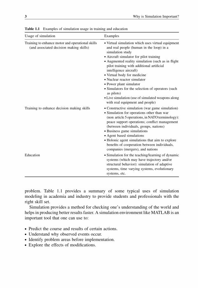
problem. Table 1.1 provides a summary of some typical uses of simulation
modeling in academia and industry to provide students and professionals with the
right skill set.
Simulation provides a method for checking one’s understanding of the world and
helps in producing better results faster. A simulation environment likeMATLAB is an
important tool that one can use to:
. Predict the course and results of certain actions.
. Understand why observed events occur.
. Identify problem areas before implementation.
. Explore the effects of modifications.
Table 1.1 Examples of simulation usage in training and education
Usage of simulation Examples
Training to enhance motor and operational skills
(and associated decision making skills)
. Virtual simulation which uses virtual equipment
and real people (human in the loop) in a
simulation study. Aircraft simulator for pilot training. Augmented reality simulation (such as in flight
pilot training with additional artificial
intelligence aircraft). Virtual body for medicine. Nuclear reactor simulator. Power plant simulator. Simulators for the selection of operators (such
as pilots). Live simulation (use of simulated weapons along
with real equipment and people)
Training to enhance decision making skills . Constructive simulation (war game simulation). Simulation for operations other than war
(non article 5 operations, inNATO terminology):
peace support operations; conflict management
(between individuals, groups, nations). Business game simulations. Agent based simulations. Holonic agent simulations that aim to explore
benefits of cooperation between individuals,
companies (mergers), and nations
Education . Simulation for the teaching/learning of dynamic
systems (which may have trajectory and/or
structural behavior): simulation of adaptive
systems, time varying systems, evolutionary
systems, etc.
3 Why is Simulation Important?

. Confirm that all variables are known.
. Evaluate ideas and identify inefficiencies.
. Gain insight and stimulate creative thinking.
. Communicate the integrity and feasibility of one’s plans.
One can use simulation when the analytical solution does not exist, is too
complicated, or requires more computational time than the simulation. Simulation
should not be used in the following cases:
. The simulation requires months or years of CPU time. In this scenario, it is probably
not feasible to run simulations.. The analytical solution exists and is simple. In this scenario, it is easier to use the
analytical solution to solve the problem rather than use simulation (unless onewants
to relax some assumptions or compare the analytical solution to the simulation).
1.2 What is a Model?
A computer model is a computer program that attempts to simulate an abstract model
of a particular system. Computer models can be classified according to several
orthogonal binary criteria including:
. Continuous state or discrete state: If the state variables of the system can assume
any value, then the system is modeled using a continuous-state model. On the other
hand, a model in which the state variables can assume only discrete values is called a
discrete-state model. Discrete-state models can be continuous- or discrete-time
models.. Continuous-time or discrete-time models: If the state variables of the system
can change their values at any instant in time, then the system can be modeled by a
continuous-time model. On the other hand, a model in which the state variables
can change their values only at discrete instants of time is called adiscrete-timemodel.
A continuous simulation uses differential equations (either partial or ordinary),
implemented numerically. Periodically, the simulation program solves all the equa-
tions, and uses the numbers to change the state and output of the simulation.Most flight
and racing-car simulations are of this type. It may also be used to simulate electric
circuits. Originally, these kinds of simulations were actually implemented on analog
computers, where the differential equations could be represented directly by various
electrical components such as op-amps. By the late 1980s, however, most “analog”
simulations were run on conventional digital computers that emulated the behavior of
an analog computer.
Basic Concepts and Techniques 4
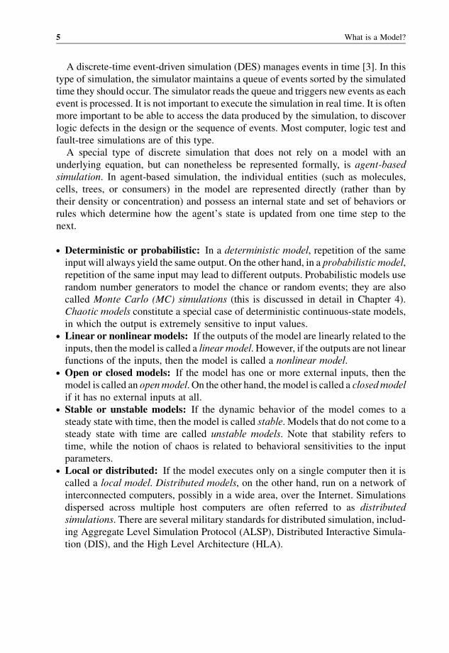
A discrete-time event-driven simulation (DES) manages events in time [3]. In this
type of simulation, the simulator maintains a queue of events sorted by the simulated
time they should occur. The simulator reads the queue and triggers new events as each
event is processed. It is not important to execute the simulation in real time. It is often
more important to be able to access the data produced by the simulation, to discover
logic defects in the design or the sequence of events. Most computer, logic test and
fault-tree simulations are of this type.
A special type of discrete simulation that does not rely on a model with an
underlying equation, but can nonetheless be represented formally, is agent-based
simulation. In agent-based simulation, the individual entities (such as molecules,
cells, trees, or consumers) in the model are represented directly (rather than by
their density or concentration) and possess an internal state and set of behaviors or
rules which determine how the agent’s state is updated from one time step to the
next.
. Deterministic or probabilistic: In a deterministic model, repetition of the same
input will always yield the same output. On the other hand, in a probabilistic model,
repetition of the same input may lead to different outputs. Probabilistic models use
random number generators to model the chance or random events; they are also
called Monte Carlo (MC) simulations (this is discussed in detail in Chapter 4).
Chaotic models constitute a special case of deterministic continuous-state models,
in which the output is extremely sensitive to input values.. Linear or nonlinear models: If the outputs of the model are linearly related to the
inputs, then the model is called a linear model. However, if the outputs are not linear
functions of the inputs, then the model is called a nonlinear model.. Open or closed models: If the model has one or more external inputs, then the
model is called an openmodel. On the other hand, themodel is called a closedmodel
if it has no external inputs at all.. Stable or unstable models: If the dynamic behavior of the model comes to a
steady state with time, then the model is called stable. Models that do not come to a
steady state with time are called unstable models. Note that stability refers to
time, while the notion of chaos is related to behavioral sensitivities to the input
parameters.. Local or distributed: If the model executes only on a single computer then it is
called a local model. Distributed models, on the other hand, run on a network of
interconnected computers, possibly in a wide area, over the Internet. Simulations
dispersed across multiple host computers are often referred to as distributed
simulations. There are several military standards for distributed simulation, includ-
ing Aggregate Level Simulation Protocol (ALSP), Distributed Interactive Simula-
tion (DIS), and the High Level Architecture (HLA).
5 What is a Model?
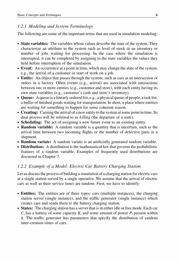
1.2.1 Modeling and System Terminology
The following are some of the important terms that are used in simulation modeling:
. State variables: The variables whose values describe the state of the system. They
characterize an attribute in the system such as level of stock in an inventory or
number of jobs waiting for processing. In the case where the simulation is
interrupted, it can be completed by assigning to the state variables the values they
held before interruption of the simulation.. Event: An occurrence at a point in time, which may change the state of the system,
e.g., the arrival of a customer or start of work on a job.. Entity: An object that passes through the system, such as cars at an intersection or
orders in a factory. Often events (e.g., arrival) are associated with interactions
between one or more entities (e.g., customer and store), with each entity having its
own state variables (e.g., customer’s cash and store’s inventory).. Queue: Aqueue is a linearly ordered list, e.g., a physical queue of people, a task list,
a buffer of finished goods waiting for transportation. In short, a place where entities
are waiting for something to happen for some coherent reason.. Creating: Causing the arrival of a new entity to the system at some point in time. Its
dual process will be referred to as killing (the departure of a state).. Scheduling: The act of assigning a new future event to an existing entity.. Random variable: A random variable is a quantity that is uncertain, such as the
arrival time between two incoming flights or the number of defective parts in a
shipment.. Random variate: A random variate is an artificially generated random variable.. Distribution: A distribution is the mathematical law that governs the probabilistic
features of a random variable. Examples of frequently used distributions are
discussed in Chapter 7.
1.2.2 Example of a Model: Electric Car Battery Charging Station
Let us discuss the process of building a simulation of a charging station for electric cars
at a single station served by a single operative. We assume that the arrival of electric
cars as well as their service times are random. First, we have to identify:
. Entities: The entities are of three types: cars (multiple instances), the charging
station server (single instance), and the traffic generator (single instance) which
creates cars and sends them to the battery charging station.. States: The charging station has a server that is in either idle or free mode. Each car
Ci has a battery of some capacity Ki and some amount of power Pi present within
it. The traffic generator has parameters that specify the distribution of random
inter-creation times of cars.
Basic Concepts and Techniques 6
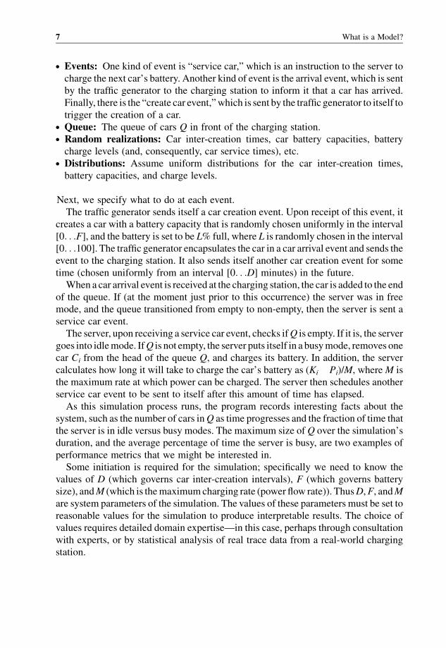
. Events: One kind of event is “service car,” which is an instruction to the server to
charge the next car’s battery. Another kind of event is the arrival event, which is sent
by the traffic generator to the charging station to inform it that a car has arrived.
Finally, there is the “create car event,”which is sent by the traffic generator to itself to
trigger the creation of a car.. Queue: The queue of cars Q in front of the charging station.. Random realizations: Car inter-creation times, car battery capacities, battery
charge levels (and, consequently, car service times), etc.. Distributions: Assume uniform distributions for the car inter-creation times,
battery capacities, and charge levels.
Next, we specify what to do at each event.
The traffic generator sends itself a car creation event. Upon receipt of this event, it
creates a car with a battery capacity that is randomly chosen uniformly in the interval
[0. . .F], and the battery is set to be L% full, where L is randomly chosen in the interval
[0. . .100]. The traffic generator encapsulates the car in a car arrival event and sends theevent to the charging station. It also sends itself another car creation event for some
time (chosen uniformly from an interval [0. . .D] minutes) in the future.
When a car arrival event is received at the charging station, the car is added to the end
of the queue. If (at the moment just prior to this occurrence) the server was in free
mode, and the queue transitioned from empty to non-empty, then the server is sent a
service car event.
The server, upon receiving a service car event, checks ifQ is empty. If it is, the server
goes into idlemode. IfQ is not empty, the server puts itself in a busymode, removes one
car Ci from the head of the queue Q, and charges its battery. In addition, the server
calculates how long it will take to charge the car’s battery as (Ki�Pi)/M, whereM is
the maximum rate at which power can be charged. The server then schedules another
service car event to be sent to itself after this amount of time has elapsed.
As this simulation process runs, the program records interesting facts about the
system, such as the number of cars inQ as time progresses and the fraction of time that
the server is in idle versus busy modes. The maximum size of Q over the simulation’s
duration, and the average percentage of time the server is busy, are two examples of
performance metrics that we might be interested in.
Some initiation is required for the simulation; specifically we need to know the
values of D (which governs car inter-creation intervals), F (which governs battery
size), andM (which is themaximumcharging rate (power flow rate)). ThusD,F, andM
are system parameters of the simulation. The values of these parameters must be set to
reasonable values for the simulation to produce interpretable results. The choice of
values requires detailed domain expertise—in this case, perhaps through consultation
with experts, or by statistical analysis of real trace data from a real-world charging
station.
7 What is a Model?
Once these event-driven behaviors are defined, they can be translated into code. This
is easywith an appropriate library that has subroutines for the creation, scheduling, and
proper timing of events, queue manipulations, random variable generation, and
collecting statistics. This charging station system will be implemented as a case
study in Chapter 4, using a discrete-event simulation framework that will be designed
and implemented in Chapter 2.
The performancemeasures (maximum size ofQ over the simulation’s duration, and
the average percentage of time the server is busy) depend heavily on random choices
made in the course of the simulation. Thus, the system is non-deterministic and the
performance measures are themselves random variables. The distributions of these
randomvariables using techniques such asMonteCarlo simulationwill be discussed in
Chapter 4.
1.3 Performance Evaluation Techniques
Modeling deals with the representation of interconnected subsystems and subpro-
cesses with the eventual objective of obtaining an estimate of an aggregate systemic
property, or performance measure. The mechanism by which one can obtain this
estimate (1) efficiently and (2) with confidence is the subject of performance
evaluation. In this section, we will lay out the methodological issues that lie therein.
A performance evaluation technique (PET) is a set of assumptions and analytical
processes (applied in the context of a simulation), whose purpose is the efficient
estimation of some performance measure. PETs fall into two broad classes: (1) direct
measurement and (2) modeling:
1. Directmeasurement: Themost obvious technique to evaluate the performance of
a system. However, limitations exist in the available traffic measurements because
of the following reasons:
(a) The direct measurement of a system is only available with operational
systems. Direct measurement is not feasible with systems under design and
development.
(b) Direct measurement of the system may affect the measured system while
obtaining the required data. This may lead to false measurements of the
measured system.
(c) It may not be practical to measure directly the level of end-to-end performance
sustained on all paths of the system. Hence, to obtain the performance
objectives, analyticalmodels have to be set up to convert the rawmeasurements
into meaningful performance measures.
2. Modeling: During the design and development phases of a system, modeling can
be used to estimate the performance measures to be obtained when the system is
Basic Concepts and Techniques 8
implemented. Modeling can be used to evaluate the performance of a working
system, especially after the system undergoes some modifications. Modeling does
not affect themeasured system as it does in the direct measurement technique and it
can be used during the design phases. However, modeling suffers from the
following problems:
(a) The problem of system abstraction. This may lead to analyzing a model that
does not represent the real system under evaluation.
(b) Problems in representing the workload of the system.
(c) Problems in obtaining performance measures for the model and mapping the
results back to the real system.
Needless to say, the direct measurement of physical systems is not the subject of this
book. Even within the modeling, only a sub-branch is considered here. To see where
this sub-branch lies, it should be noted that at the heart of every model is its formal
description. This can almost always be given in terms of a collection of interconnected
queues. Once a system has been modeled as a collection of interconnected queues,
there are two broadly defined approaches for determining actual performance mea-
sures: (1) analytical modeling and (2) simulation modeling. Analytical modeling of
such a system seeks to deduce the parameters throughmathematical derivation, and so
leads into the domain of queuing theory—a fascinating mathematical subject for
which many texts are already available. In contrast, simulation modeling (which is the
subject of this book) determines performance measures by making direct measure-
ments of a simplified virtual system that has been created through computational
means.
In simulation modeling, there are few PETs that can be applied generally, though
many PETs are based on modifications of the so-called Monte Carlo method that will
be discussed in depth in Chapter 4. More frequently, each PET typically has to be
designed on a case-by-case basis given the system at hand. The process of defining a
PET involves:
1. Assumptions or simplifications of the properties of the atomic elements within a
system and the logic underlying their evolution through interactions.2
2. Statistical assumptions on the properties of non-deterministic aspects of the system,
e.g., its constituent waveforms.
3. Statistical techniques for aggregating performance measure estimates obtained
from disparate simulations of different system configurations.3
2 Note that this implies that a PET may be intertwined with the process of model construction, and because of this,
certain PETs imply or require departure from an established model.3 At the simplest level, we can consider Monte Carlo simulation to be a PET. It satisfies our efficiency objective to the
extent that the computations associatedwith missing or simplified operations reduce the overall computational burden.
9 Performance Evaluation Techniques
To illustrate, let us consider an example of a PETmethodology thatmight be applied
in the study of a high data rate system over slowly fading channels.Without going into
too many details, such a system’s performance depends upon two random processes
with widely different rates of change in time. One of the processes is “fast” in terms of
its dynamismwhile the other is “slow.” For example, the fast process in this casemight
be thermal noise, while the slow process might be signal fading. If the latter process is
sufficiently slow relative to the first, then it can be approximated as being considered
fixed with respect to the fast process. In such a system, the evolution of a received
waveform could be simulated, by considering a sequence of time segments over each
of which the state of the slow process is different, but fixed. We might simulate such a
sequence of segments, and view each segment as being an experiment (conditioned on
the state of the slow process) and obtain conditional performance metrics. The final
performance measure estimate might then be taken as the average over these
conditional estimates. This narrative illustrates the process of selecting and specifying
a PET.
1.3.1 Example of Electric Car Battery Charging Station
In Section 1.2.1, a model of a charging station was described. What might the
associated performance measures be when we simulate the model? There are many
possible interesting aggregate performance measures we could consider, such as the
number of cars inQ as time progresses and the fraction of timewhen the server is in idle
versus busy modes.
1.3.1.1 Practical Considerations
Simulation is, in some sense, an act of pretending that one is dealing with a real
object when actually one is working with an imitation of reality. It may beworthwhile
to consider when such pretense is warranted, and the benefits/dangers of engaging
in it.
1.3.1.2 Why Use Models?
Models reduce cost using different simplifying assumptions.A spacecraft simulator on
a certain computer (or simulator system) is also a computer model of some aspects of
the spacecraft. It shows on the computer screen the controls and functions that the
spacecraft user is supposed to seewhen using the spacecraft. To train individuals using
a simulator is more convenient, safer, and cheaper than a real spacecraft that usually
cost billions of dollars. It is prohibitive (and impossible) to use a real spacecraft as a
Basic Concepts and Techniques 10
training system. Therefore, industry, commerce, and the military often use models
rather than real experiments. Real experiments can be as costly and dangerous as real
systems so, provided that models are adequate descriptions of reality, they can give
results that are closer to those achieved by a real system analysis.
1.3.1.3 When to Use Simulations?
Simulation is used in many situations, such as:
1. When the analytical model/solution is not possible or feasible. In such cases,
experts resort to simulations.
2. Many times, simulation results are used to verify analytical solutions in order to
make sure that the system is modeled correctly using analytical approaches.
3. Dynamic systems, which involve randomness and change of state with time. An
example is our electric car charging station where cars come and go unpredictably
to charge their batteries. In such systems, it is difficult (sometimes impossible) to
predict exactly what time the next car should arrive at the station.
4. Complex dynamic systems, which are so complex that when analyzed theoretically
will require too many simplifications. In such cases, it is not possible to study the
system and analyze it analytically. Therefore, simulation is the best approach to
study the behavior of such a complex system.
1.3.1.4 How to Simulate?
Suppose one is interested in studying the performance of an electric car charging
station (the example treated above). The behavior of this system may be described
graphically by plotting the number of cars in the charging station and the state of the
system. Every time a car arrives, the graph increases by one unit, while a departing car
causes the graph to drop one unit. This graph, also called a sample path, could be
obtained from observation of a real electric car charging station, but could also be
constructed artificially. Such artificial construction and the analysis of the resulting
sample path (or more sample paths in more complex cases) constitute the simulation
process.
1.3.1.5 How Is Simulation Performed?
Simulations may be performed manually (on paper for instance). More frequently,
however, the systemmodel is written either as a computer program or as some kind of
input to simulation software, as shown in Figure 1.1.
11 Performance Evaluation Techniques

Start
End
Iteration = 0
Read Input () Write Output () Initialization () Print Status ()
++ Iteration Timing ()
Print Status ()
Event Type = Type 1
Event Type = Type 3
Event Type = Type 2
Event Type = Type 4
Generated Cells < Required Cells
Event Type = Type 5
Event routine of Type 1
Event routine of Type 2
Event routine of Type 3
Event routine of Type 4
Event routine of Type 5
Report Generation
Figure 1.1 Overall structure of a simulation program
Basic Concepts and Techniques 12
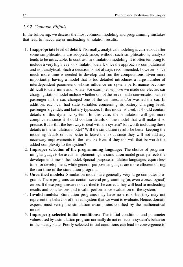
1.3.2 Common Pitfalls
In the following, we discuss the most common modeling and programming mistakes
that lead to inaccurate or misleading simulation results:
1. Inappropriate level of detail: Normally, analytical modeling is carried out after
some simplifications are adopted, since, without such simplifications, analysis
tends to be intractable. In contrast, in simulation modeling, it is often tempting to
include a very high level of simulation detail, since the approach is computational
and not analytical. Such a decision is not always recommended, however, since
much more time is needed to develop and run the computations. Even more
importantly, having a model that is too detailed introduces a large number of
interdependent parameters, whose influence on system performance becomes
difficult to determine and isolate. For example, suppose we made our electric car
charging stationmodel includewhether or not the server had a conversation with a
passenger in the car, changed one of the car tires, and/or washed the car. In
addition, each car had state variables concerning its battery charging level,
passenger’s gender, and battery type/size. If this model is used, it should contain
details of this dynamic system. In this case, the simulation will get more
complicated since it should contain details of the model that will make it so
precise. But is this the best way to deal with the system? Is it worth including these
details in the simulation model? Will the simulation results be better keeping the
modeling details or it is better to leave them out since they will not add any
necessary improvements to the results? Even if they do, will that be worth the
added complexity to the system?
2. Improper selection of the programming language: The choice of program-
ming language to be used in implementing the simulationmodel greatly affects the
development time of themodel. Special-purpose simulation languages require less
time for development, while general-purpose languages are more efficient during
the run time of the simulation program.
3. Unverified models: Simulation models are generally very large computer pro-
grams. These programs can contain several programming (or, evenworse, logical)
errors. If these programs are not verified to be correct, theywill lead to misleading
results and conclusions and invalid performance evaluation of the system.
4. Invalid models: Simulation programs may have no errors, but they may not
represent the behavior of the real system that wewant to evaluate. Hence, domain
experts must verify the simulation assumptions codified by the mathematical
model.
5. Improperly selected initial conditions: The initial conditions and parameter
values used by a simulation program normally do not reflect the system’s behavior
in the steady state. Poorly selected initial conditions can lead to convergence to
13 Performance Evaluation Techniques

atypical steady states, suggesting misleading conclusions about the system. Thus,
domain experts must verify the initial conditions and parameters before they are
used within the simulation program.
6. Short run times: System analysts may try to save time by running simulation
programs for short periods. Short runs lead to false results that are strongly
dependent on the initial conditions and thus do not reflect the true performance of
the system in typical steady-state conditions.
7. Poor random number generators: Random number generators employed in
simulation programs can greatly affect simulation results. It is important to use a
randomnumbergenerator that has been extensively tested and analyzed. The seeds
that are supplied to the random number generator should also be selected to ensure
that there is no correlation between the different processes in the system.
8. Inadequate time estimate: Most simulation models fail to give an adequate
estimate of time needed for the development and implementation of the simulation
model. The development, implementation, and testing of a simulation model
require a great deal of time and effort.
9. No achievable goals: Simulation models may fail because no specific, achiev-
able goals are set before beginning the process of developing the simulation
model.
10. Incomplete mix of essential skills: For a simulation project to be successful, it
should employ personnelwho have different types of skills, such as project leaders
and programmers, people who have skills in statistics and modeling, and people
who have a good domain knowledge and experience with the actual system being
modeled.
11. Inadequate level of user participation: Simulation models that are developed
without end user’s participation are usually not successful. Regular meetings
among end users, system developers, and system implementers are important for a
successful simulation program.
12. Inability to manage the simulation project: Most simulation projects are
extremely complex, so it is important to employ software engineering tools to
keep track of the progress and functionality of a project.
1.3.3 Types of Simulation Techniques
The most important types of simulations described in the literature that are of special
importance to engineers are:
1. Emulation: The process of designing and building hardware or firmware
(i.e., prototype) that imitates the functionality of the real system.
2. Monte Carlo simulation: Any simulation that has no time axis. Monte Carlo
simulation is used to model probabilistic phenomena that do not change with time,
Basic Concepts and Techniques 14
or to evaluate non-probabilistic expressions using probabilistic techniques. This
kind of simulation will be discussed in greater detail in Chapter 4.
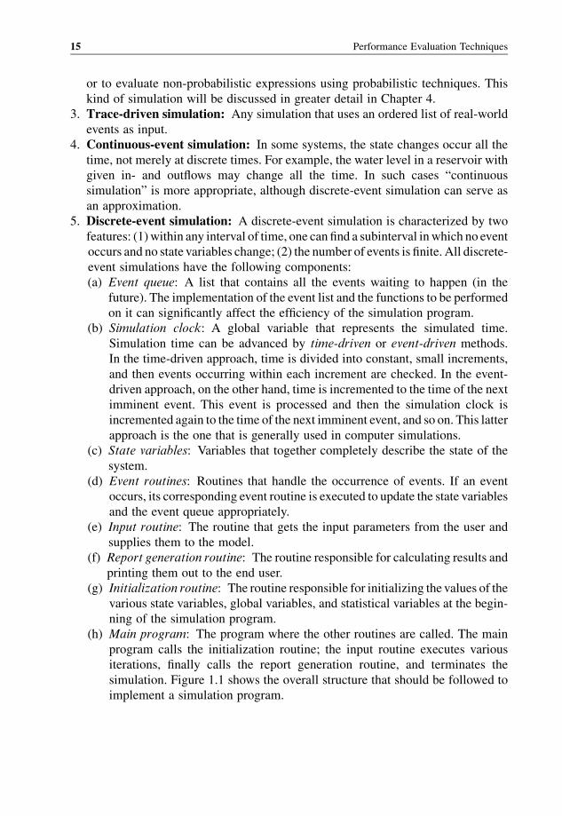
3. Trace-driven simulation: Any simulation that uses an ordered list of real-world
events as input.
4. Continuous-event simulation: In some systems, the state changes occur all the
time, not merely at discrete times. For example, the water level in a reservoir with
given in- and outflows may change all the time. In such cases “continuous
simulation” is more appropriate, although discrete-event simulation can serve as
an approximation.
5. Discrete-event simulation: A discrete-event simulation is characterized by two
features: (1)within any interval of time, one can find a subinterval inwhich no event
occurs and no state variables change; (2) the number of events is finite. All discrete-
event simulations have the following components:
(a) Event queue: A list that contains all the events waiting to happen (in the
future). The implementation of the event list and the functions to be performed
on it can significantly affect the efficiency of the simulation program.
(b) Simulation clock: A global variable that represents the simulated time.
Simulation time can be advanced by time-driven or event-driven methods.
In the time-driven approach, time is divided into constant, small increments,
and then events occurring within each increment are checked. In the event-
driven approach, on the other hand, time is incremented to the time of the next
imminent event. This event is processed and then the simulation clock is
incremented again to the time of the next imminent event, and so on. This latter
approach is the one that is generally used in computer simulations.
(c) State variables: Variables that together completely describe the state of the
system.
(d) Event routines: Routines that handle the occurrence of events. If an event
occurs, its corresponding event routine is executed to update the state variables
and the event queue appropriately.
(e) Input routine: The routine that gets the input parameters from the user and
supplies them to the model.
(f) Report generation routine: The routine responsible for calculating results and
printing them out to the end user.
(g) Initialization routine: The routine responsible for initializing the values of the
various state variables, global variables, and statistical variables at the begin-
ning of the simulation program.
(h) Main program: The program where the other routines are called. The main
program calls the initialization routine; the input routine executes various
iterations, finally calls the report generation routine, and terminates the
simulation. Figure 1.1 shows the overall structure that should be followed to
implement a simulation program.
15 Performance Evaluation Techniques
1.4 Development of Systems Simulation
Discrete-event systems are dynamic systems that evolve in time by the occurrence of
events at possibly irregular time intervals. Examples include traffic systems, flexible
manufacturing systems, computer communications systems, production lines, coher-
ent lifetime systems, and flow networks. Most of these systems can be modeled in
terms of discrete events whose occurrence causes the system to change state. In
designing, analyzing, and simulating such complex systems, one is interested not only
in performance evaluation, but also in analysis of the sensitivity of the system to design
parameters and optimal selection of parameter values.
A typical stochastic system has a large number of control parameters, each of
which can have a significant impact on the performance of the system. An overarching
objective of simulation is to determine the relationship between system behavior and
input parameter values, and to estimate the relative importance of these parameters and
their relationships to one another as mediated by the system itself. The technique
by which this information is deduced is termed sensitivity analysis. The methodology
is to apply small perturbations to the nominal values of input parameters and observe
the effects on system performance measures. For systems simulation, variations of
the input parameter values cannot be made infinitely small (since this would then
require an infinite number of simulations to be conducted). The sensitivity (of the
performance measure with respect to an input parameter) is taken to be an approxi-
mation of the partial derivative of the performance measure with respect to the
parameter value.
The development process of system simulation involves some or all of the following
stages:
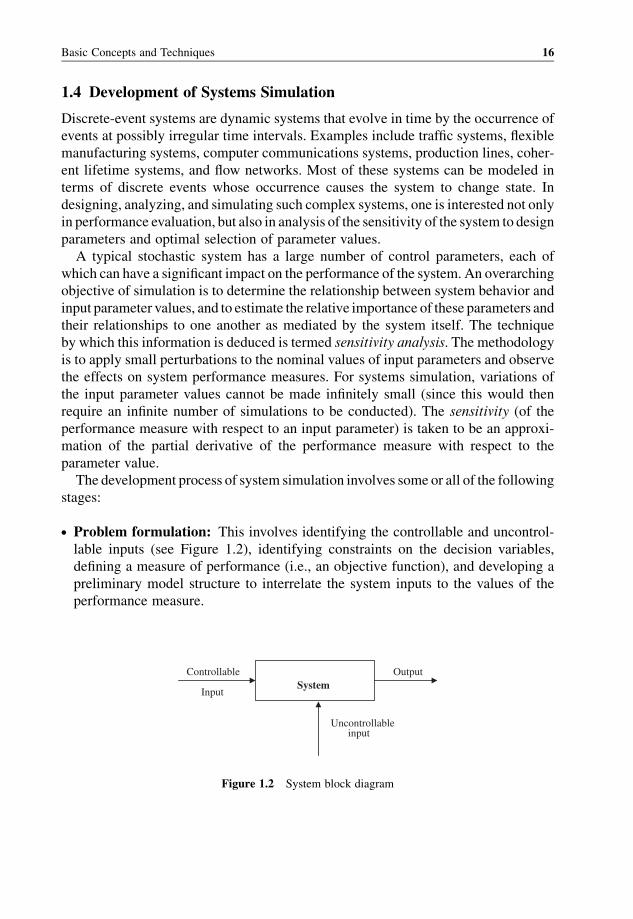
. Problem formulation: This involves identifying the controllable and uncontrol-
lable inputs (see Figure 1.2), identifying constraints on the decision variables,
defining a measure of performance (i.e., an objective function), and developing a
preliminary model structure to interrelate the system inputs to the values of the
performance measure.
SystemControllable
Input
Output
Uncontrollable input
Figure 1.2 System block diagram
Basic Concepts and Techniques 16
. Data collection and analysis: Decide what data to collect about the real system,
and how much to collect. This decision is a tradeoff between cost and accuracy.. Simulationmodel development: Acquire sufficient understanding of the system to
develop an appropriate conceptual, logical model of the entities and their states, as
well as the events codifying the interactions between entities (and time). This is the
heart of simulation design.. Model validation, verification, and calibration: In general, verification focuses
on the internal consistency of a model, while validation is concerned with the
correspondence between the model and the reality. The term validation is applied to
those processes that seek to determine whether or not a simulation is correct with
respect to the “real” system. More precisely, validation is concerned with the
question “arewe building the right system?”Verification, on the other hand, seeks to
answer the question “are we building the system right?” Verification checks that the
implementation of the simulation model (program) corresponds to the model.
Validation checks that the model corresponds to reality. Finally, calibration checks
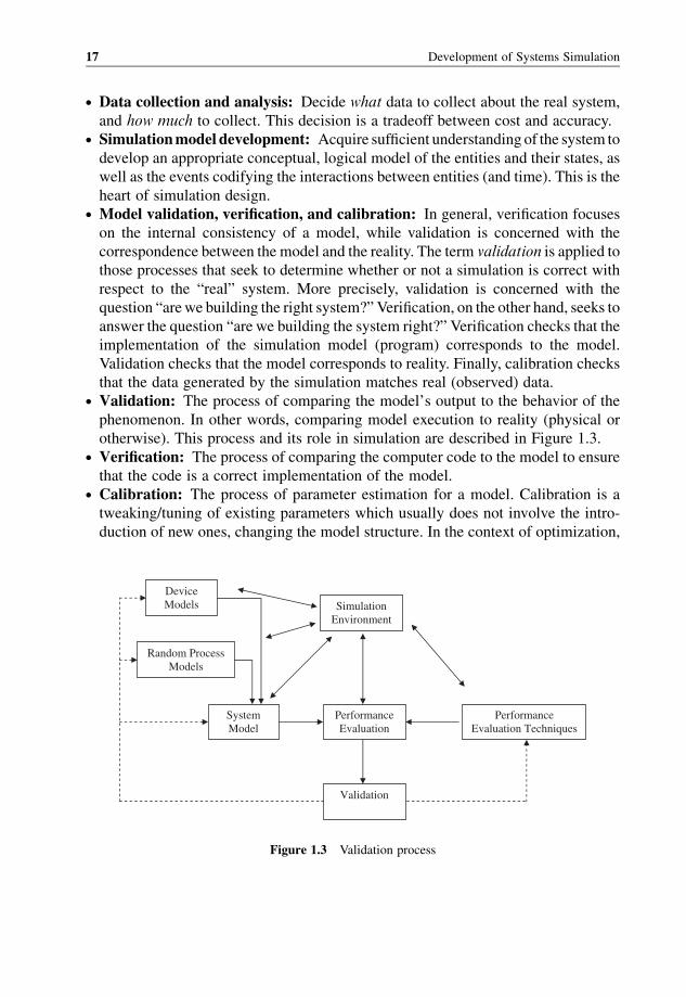
that the data generated by the simulation matches real (observed) data.. Validation: The process of comparing the model’s output to the behavior of the
phenomenon. In other words, comparing model execution to reality (physical or
otherwise). This process and its role in simulation are described in Figure 1.3.. Verification: The process of comparing the computer code to the model to ensure
that the code is a correct implementation of the model.. Calibration: The process of parameter estimation for a model. Calibration is a
tweaking/tuning of existing parameters which usually does not involve the intro-
duction of new ones, changing the model structure. In the context of optimization,
Simulation Environment
DeviceModels
Random Process Models
System Model
Performance Evaluation
Performance Evaluation Techniques
Validation
Figure 1.3 Validation process
17 Development of Systems Simulation
calibration is an optimization procedure involved in system identification or during
the experimental design.. Input and output analysis: Discrete-event simulation models typically have
stochastic components that mimic the probabilistic nature of the system under
consideration. Successful input modeling requires a close match between the input
model and the true underlying probabilistic mechanism associated with the system.
The input data analysis is tomodel an element (e.g., arrival process, service times) in
a discrete-event simulation given a data set collected on the element of interest. This
stage performs intensive error checking on the input data, including external, policy,
random, and deterministic variables. System simulation experiments aim to learn
about its behavior. Careful planning, or designing, of simulation experiments is
generally a great help, saving time and effort by providing efficient ways to estimate
the effects of changes in the model’s inputs on its outputs. Statistical experimental
design methods are mostly used in the context of simulation experiments.. Performance evaluation and “what-if” analysis: The “what-if” analysis involves
trying to run the simulation with different input parameters (i.e., under different
“scenarios”) to see how performance measures are affected.. Sensitivity estimation: Users must be provided with affordable techniques for
sensitivity analysis if they are to understand the relationships and tradeoffs between
system parameters and performancemeasures in ameaningful way that allows them
to make good system design decisions.. Optimization: Traditional optimization techniques require gradient estimation. As
with sensitivity analysis, the current approach for optimization requires intensive
simulation to construct an approximate surface response function. Sophisticated
simulations incorporate gradient estimation techniques into convergent algorithms
such as Robbins–Monroe in order to efficiently determine system parameter values
which optimize performance measures. There are many other gradient estimation
(sensitivity analysis) techniques, including: local information, structural properties,
response surface generation, the goal-seeking problem, optimization, the “what-if”
problem, and meta-modeling.. Report generating: Report generation is a critical link in the communication
process between the model and the end user.
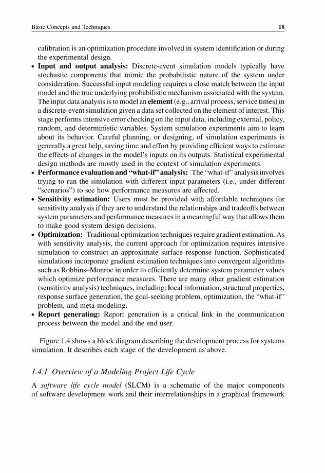
Figure 1.4 shows a block diagram describing the development process for systems
simulation. It describes each stage of the development as above.
1.4.1 Overview of a Modeling Project Life Cycle
A software life cycle model (SLCM) is a schematic of the major components
of software development work and their interrelationships in a graphical framework
Basic Concepts and Techniques 18
that can be easily understood and communicated. The SLCM partitions the work to be
done into manageable work units. Having a defined SLCM for your project allows
you to:
1. Define the work to be performed.
2. Divide up the work into manageable pieces.
3. Determine project milestones at which project performance can be evaluated.
4. Define the sequence of work units.
5. Provide a framework for definition and storage of the deliverables produced during
the project.
6. Communicate your development strategy to project stakeholders.
An SLCM achieves this by:
1. Providing a simple graphical representation of the work to be performed.
Validated, Verified Base Model
Goal Seeking Problem
Optimization Problem
Stability and the What-If-Analysis
1. Descriptive Analysis
2. Prescriptive Analysis
3. Post-Prescriptive Analysis
Figure 1.4 Development process for simulation
19 Development of Systems Simulation
2. Allowing focus on important features of the work, downplaying excessive
detail.
3. Providing a standardwork unit hierarchy for progressivedecomposition of thework
into manageable chunks.
4. Providing for changes (tailoring) at low cost.
Before specifying how this is achieved, we need to classify the life cycle processes
dealing with the software development process.
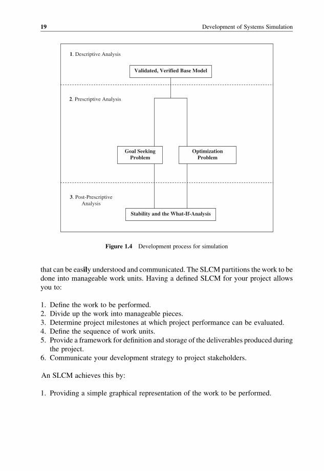
1.4.2 Classifying Life Cycle Processes
Figure 1.5 shows the three main classes of a software development process and gives
examples of the members of each class:
. Project support processes: are involved with the management of the software
development exercise. They are performed throughout the life of the project.. Development processes: embody all work that directly contributes to the devel-
opment of the project deliverable. They are typically interdependent.. Integral processes: are common processes that are performed in the context of
more than one development activity. For example, the reviewprocess is performed in
the context of requirements definition, design, and coding.
SoftwareDevelopmentProcesses
Project Support Processes
Development Processes
Integral Processes
Project Management
Quality Management
Configuration Management
Concept
Requirements
Design
Coding
Testing
Installation
MaintenanceRetirement
Planning
Training
Review
Problem Resolution
Risk Management
Document Management
Interview
Joint Session
Technical Investigation
Test
Figure 1.5 Software life cycle process classifications
Basic Concepts and Techniques 20
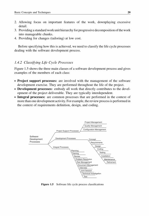
1.4.3 Describing a Process
Processes are described in terms of a series of work units. Work units are logically
related chunks ofwork. For example, all preliminary design effort is naturally chunked
together. Figure 1.6 describes the components of a work unit.
A work unit is described in terms of:
. Work flow input/output: Work flows are the work products that flow from one
work unit to the next. For example, in Figure 1.6, the design specification flows from
the output of the design work unit to the input of the code work unit. Work flows are
the deliverables from the work unit. All work units must have a deliverable. The life
cycle model should provide detailed descriptions of the format and content of all
deliverables.. Entry criteria: The conditions that must exist before a work unit can commence.. Statement of work (SOW): The SOW describes the work to be performed on the
work flow inputs to create the outputs.. Exit criteria: The conditions that must exist for the work to be deemed complete.
The above terms are further explained through the usage of examples in Table 1.2.
Feedback paths are the paths by which work performed in one work unit impacts
work either in progress or completed in a precedingwork unit. For example, themodel
depicted in Figure 1.7 allows for the common situation where the act of coding often
uncovers inconsistencies and omissions in the design. The issues raised by program-
mers then require a reworking of the baseline design document.
Defining feedback paths provides a mechanism for iterative development of work
products. That is, it allows for the real-world fact that specifications and code are
seldom complete and correct at their first approval point. The feedback path allows for
planning, quantification, and control of the rework effort. Implementing feedback
paths on a project requires the following procedures:
1. A procedure to raise issues or defects with baseline deliverables.
2. A procedure to review issues and approve rework of baseline deliverables.
3. Allocation of budget for rework in each project phase.
EntryCriteria
Statement of Work
ExitCriteria
Out In
Feedback
Work Flow Input
Work Flow Output
Figure 1.6 Components of a work unit
21 Development of Systems Simulation
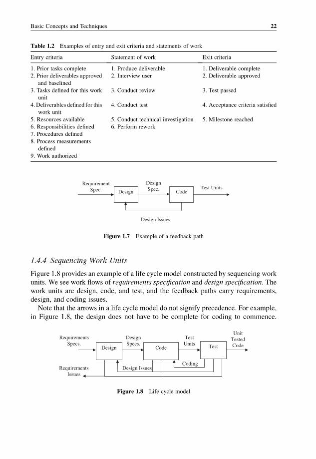
1.4.4 Sequencing Work Units
Figure 1.8 provides an example of a life cycle model constructed by sequencing work
units. We see work flows of requirements specification and design specification. The
work units are design, code, and test, and the feedback paths carry requirements,
design, and coding issues.
Note that the arrows in a life cycle model do not signify precedence. For example,
in Figure 1.8, the design does not have to be complete for coding to commence.
Table 1.2 Examples of entry and exit criteria and statements of work
Entry criteria Statement of work Exit criteria
1. Prior tasks complete 1. Produce deliverable 1. Deliverable complete
2. Prior deliverables approved
and baselined
2. Interview user 2. Deliverable approved
3. Tasks defined for this work
unit
3. Conduct review 3. Test passed
4. Deliverables defined for this
work unit
4. Conduct test 4. Acceptance criteria satisfied
5. Resources available 5. Conduct technical investigation 5. Milestone reached
6. Responsibilities defined 6. Perform rework
7. Procedures defined
8. Process measurements
defined
9. Work authorized
Design Code Test
Design IssuesCoding
Requirements Specs.
UnitTestedCode
DesignSpecs.
TestUnits
Requirements Issues
Figure 1.8 Life cycle model
Design Code
Design Issues
Requirement Spec. Test Units
DesignSpec.
Figure 1.7 Example of a feedback path
Basic Concepts and Techniques 22
Design may be continuing while some unrelated elements of the system are being
coded.
1.4.5 Phases, Activities, and Tasks
A primary purpose of the life cycle model is to communicate the work to be done
among human beings. Conventional wisdom dictates that, to guarantee comprehen-
sion, a single life cycle model should therefore not have more than nine work units.
Clearly this would not be enough to describe even the simplest projects.
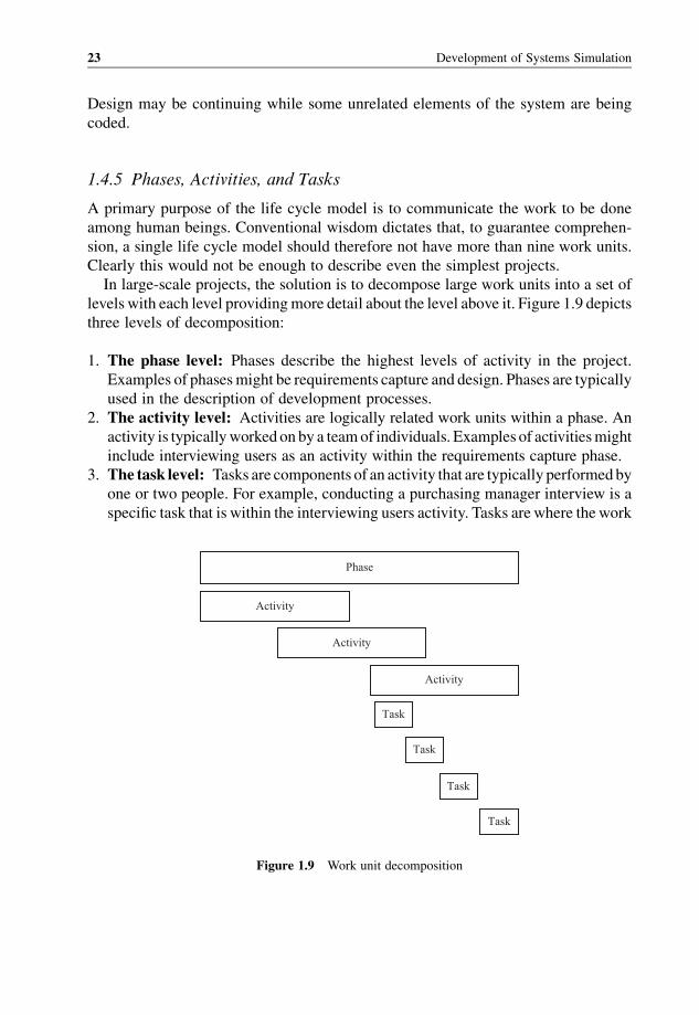
In large-scale projects, the solution is to decompose large work units into a set of
levels with each level providingmore detail about the level above it. Figure 1.9 depicts
three levels of decomposition:
1. The phase level: Phases describe the highest levels of activity in the project.
Examples of phasesmight be requirements capture and design. Phases are typically
used in the description of development processes.
2. The activity level: Activities are logically related work units within a phase. An
activity is typicallyworked on by a teamof individuals. Examples of activitiesmight
include interviewing users as an activity within the requirements capture phase.
3. The task level: Tasks are components of an activity that are typically performedby
one or two people. For example, conducting a purchasing manager interview is a
specific task that is within the interviewing users activity. Tasks are where the work
Phase
Activity
Activity
Activity
Task
Task
Task
Task
Figure 1.9 Work unit decomposition
23 Development of Systems Simulation

is done. A task will have time booked to it on a time sheet. Conventional guidelines
specify that a single task should be completed in an average elapsed time of 5
working days and its duration should not exceed 15 working days.
Note that phases, activities, and tasks are all types of a work unit. You can therefore
describe them all in terms of entry criteria, statement of work, and exit criteria.
As a concrete example, Figure 1.10 provides a phase-level life cycle model for a
typical software development project.
1.5 Summary
In this chapter, we introduced the foundations of modeling and simulation.
We highlighted the importance, the needs, and the usage of simulation and modeling
in practical and physical systems. We also discussed the different approaches to
modeling that are used in practice and discussed at a high level the methodology that
should be followed when executing a modeling project.
Recommended Reading
[1] J. Sokolowski and C. Banks (Editors), Principles of Modeling and Simulation: A Multidisciplinary
Approach, John Wiley & Sons, Inc., 2009.[2] J. Banks (Editor), Handbook of Simulation: Principles, Methodology, Advances, Applications, and
Practice, John Wiley & Sons, Inc., 1998.[3] B. Zeigler, H. Praehofer, and T. G. Kim, Theory of Modeling and Simulation, 2nd Edition, Academic
Press, 2000.[4] A. Law, Simulation Modeling and Analysis, 4th Edition, McGraw Hill, 2007.
Requirements Capture
System Test Planning
Preliminary Design
Integration Test Planning
Detailed Design
Unit Test Planning
System Testing
IntegrationTesting
UnitTesting
Deployment
Maintenanceand
Enhancement
Coding
Main Work Flow
Feedback Path
Figure 1.10 A generic project model for software development
Basic Concepts and Techniques 24
2
Designing and Implementinga Discrete-Event SimulationFramework
In software engineering, the term framework is generally applied to a set of
cooperating classes that make up a reusable foundation for a specific class of
software: frameworks are increasingly important because they are the means by
which systems achieve the greatest code reuse. In this section, wewill put together a
basic discrete-event simulation framework in Java. We call this the framework for
discrete-event simulation (FDES). The framework is not large, requiring fewer than
250 lines of code, spread across just three classes, and yet, as we will see, it is an
extremely powerful organizational structure. We will deduce the design of the
simulation framework (together with its code) in the pages that follow. Then wewill
present some “toy examples” as a tutorial on how to write applications over the
framework. In the next chapter, we will consider a large case study that illustrates
the power of the framework in real-world settings. However, by looking at
everything down to the framework internals, we will have a much better under-
standing of how discrete-event simulations work. In later chapters, the framework
will be extended to support specialized constructs and primitives necessary for
network simulation.
As noted earlier, the heart of any discrete-event simulator is a “scheduler,” which
acts as the centralized authority on the passage of time. The scheduler is a repository of
future actions and is responsible for executing them sequentially. On the surface, this
might seem like a trivial task. The complication arises from the fact that each event that
is executing “now” can cause future events to be scheduled. These future events are
Network Modeling and Simulation M. Guizani, A. Rayes, B. Khan and A. Al Fuqaha
� 2010 John Wiley & Sons, Ltd.
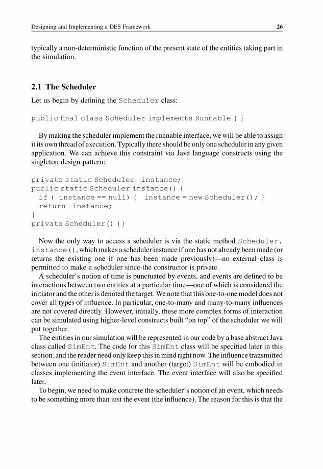
typically a non-deterministic function of the present state of the entities taking part in
the simulation.
2.1 The Scheduler
Let us begin by defining the Scheduler class:
public final class Scheduler implements Runnable { }
Bymaking the scheduler implement the runnable interface, wewill be able to assign
it its own thread of execution. Typically there should be only one scheduler in any given
application. We can achieve this constraint via Java language constructs using the
singleton design pattern:
private static Scheduler instance;
public static Scheduler instance() {
if ( instance == null) { instance = new Scheduler(); }
return instance;
}
private Scheduler() {}
Now the only way to access a scheduler is via the static method Scheduler.
instance(), whichmakes a scheduler instance if one has not already beenmade (or
returns the existing one if one has been made previously)––no external class is
permitted to make a scheduler since the constructor is private.
A scheduler’s notion of time is punctuated by events, and events are defined to be
interactions between two entities at a particular time—one of which is considered the
initiator and the other is denoted the target.We note that this one-to-onemodel does not
cover all types of influence. In particular, one-to-many and many-to-many influences
are not covered directly. However, initially, these more complex forms of interaction
can be simulated using higher-level constructs built “on top” of the scheduler we will
put together.
The entities in our simulation will be represented in our code by a base abstract Java
class called SimEnt. The code for this SimEnt class will be specified later in this
section, and the reader need only keep this inmind right now.The influence transmitted
between one (initiator) SimEnt and another (target) SimEnt will be embodied in
classes implementing the event interface. The event interface will also be specified
later.
To begin, we need to make concrete the scheduler’s notion of an event, which needs
to be something more than just the event (the influence). The reason for this is that the
Designing and Implementing a DES Framework 26
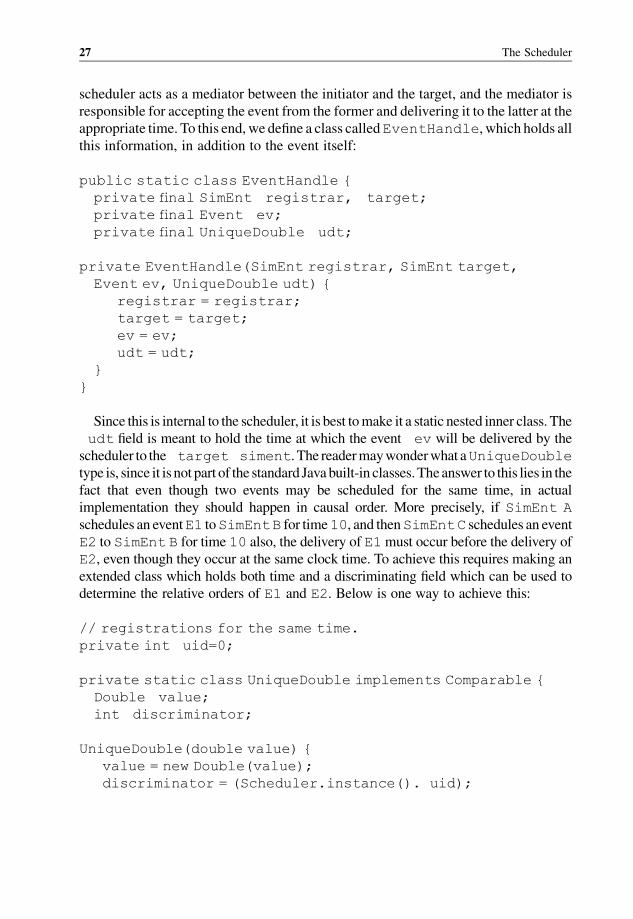
scheduler acts as a mediator between the initiator and the target, and the mediator is
responsible for accepting the event from the former and delivering it to the latter at the
appropriate time. To this end, we define a class calledEventHandle, which holds all
this information, in addition to the event itself:
public static class EventHandle {
private final SimEnt registrar, target;
private final Event ev;
private final UniqueDouble udt;
private EventHandle(SimEnt registrar, SimEnt target,
Event ev, UniqueDouble udt) {
registrar = registrar;
target = target;
ev = ev;
udt = udt;
}
}
Since this is internal to the scheduler, it is best tomake it a static nested inner class. The
udt field is meant to hold the time at which the event ev will be delivered by the
scheduler to the target siment. The readermaywonderwhat aUniqueDouble
type is, since it is not part of the standard Javabuilt-in classes.Theanswer to this lies in the
fact that even though two events may be scheduled for the same time, in actual
implementation they should happen in causal order. More precisely, if SimEnt A
schedules an eventE1 toSimEntB for time10, and thenSimEntC schedules an event
E2 to SimEnt B for time 10 also, the delivery of E1must occur before the delivery of
E2, even though they occur at the same clock time. To achieve this requires making an
extended class which holds both time and a discriminating field which can be used to
determine the relative orders of E1 and E2. Below is one way to achieve this:
// registrations for the same time.
private int uid=0;
private static class UniqueDouble implements Comparable {
Double value;
int discriminator;
UniqueDouble(double value) {
value = new Double(value);
discriminator = (Scheduler.instance(). uid);
27 The Scheduler
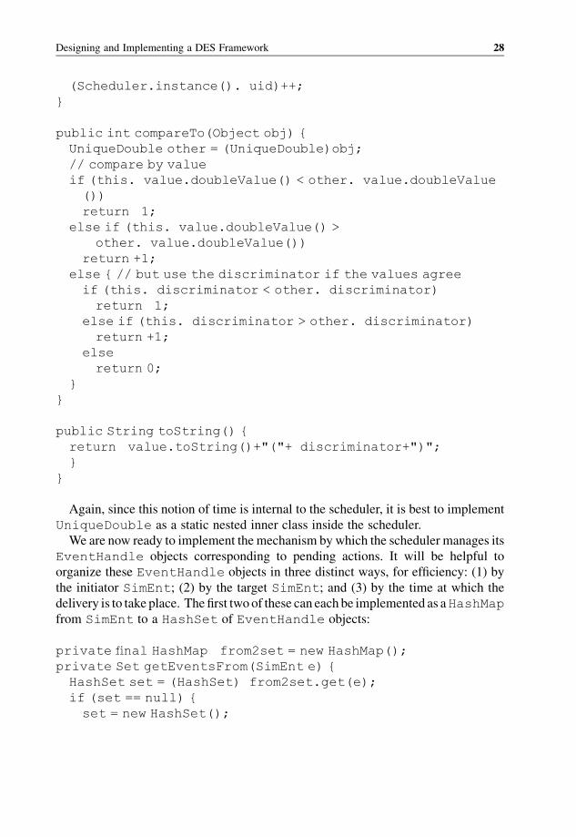
(Scheduler.instance(). uid)++;
}
public int compareTo(Object obj) {
UniqueDouble other = (UniqueDouble)obj;
// compare by value
if (this. value.doubleValue() < other. value.doubleValue
())
return 1;
else if (this. value.doubleValue() >
other. value.doubleValue())
return +1;
else { // but use the discriminator if the values agree
if (this. discriminator < other. discriminator)
return 1;
else if (this. discriminator > other. discriminator)
return +1;
else
return 0;
}
}
public String toString() {
return value.toString()+"("+ discriminator+")";
}
}
Again, since this notion of time is internal to the scheduler, it is best to implement
UniqueDouble as a static nested inner class inside the scheduler.
We are now ready to implement the mechanism by which the scheduler manages its
EventHandle objects corresponding to pending actions. It will be helpful to
organize these EventHandle objects in three distinct ways, for efficiency: (1) by
the initiator SimEnt; (2) by the target SimEnt; and (3) by the time at which the
delivery is to take place. The first twoof these can each be implemented as aHashMap
from SimEnt to a HashSet of EventHandle objects:
private final HashMap from2set = new HashMap();
private Set getEventsFrom(SimEnt e) {
HashSet set = (HashSet) from2set.get(e);
if (set == null) {
set = new HashSet();
Designing and Implementing a DES Framework 28
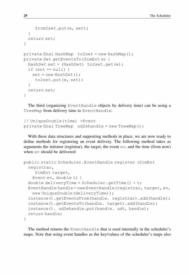
from2set.put(e, set);
}
return set;
}
private final HashMap to2set = new HashMap();
private Set getEventsTo(SimEnt e) {
HashSet set = (HashSet) to2set.get(e);
if (set == null) {
set = new HashSet();
to2set.put(e, set);
}
return set;
}
The third (organizing EventHandle objects by delivery time) can be using a
TreeMap from delivery time to EventHandle:
// UniqueDouble(time) >Event
private final TreeMap ud2ehandle = new TreeMap();
With these data structures and supporting methods in place, we are now ready to
define methods for registering an event delivery. The following method takes as
arguments the initiator (registrar), the target, the event ev, and the time (from now)
when ev should be delivered:
public static Scheduler.EventHandle register (SimEnt
registrar,
SimEnt target,
Event ev, double t) {
double deliveryTime = Scheduler.getTime() + t;
EventHandlehandle= new EventHandle(registrar, target,ev,
new UniqueDouble(deliveryTime));
instance().getEventsFrom(handle. registrar).add(handle);
instance().getEventsTo(handle. target).add(handle);
instance(). ud2ehandle.put(handle. udt, handle);
return handle;
}
The method returns the EventHandle that is used internally in the scheduler’s
maps. Note that using event handles as the key/values of the scheduler’s maps also
29 The Scheduler
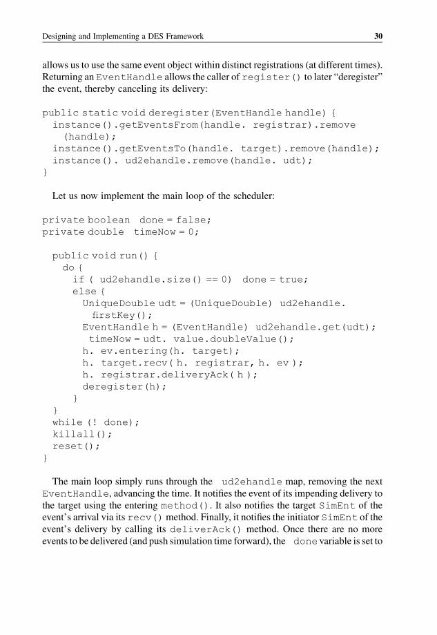
allows us to use the same event object within distinct registrations (at different times).
Returning an EventHandle allows the caller of register() to later “deregister”
the event, thereby canceling its delivery:
public static void deregister(EventHandle handle) {
instance().getEventsFrom(handle. registrar).remove
(handle);
instance().getEventsTo(handle. target).remove(handle);
instance(). ud2ehandle.remove(handle. udt);
}
Let us now implement the main loop of the scheduler:
private boolean done = false;
private double timeNow = 0;
public void run() {
do {
if ( ud2ehandle.size() == 0) done = true;
else {
UniqueDouble udt = (UniqueDouble) ud2ehandle.
firstKey();
EventHandle h = (EventHandle) ud2ehandle.get(udt);
timeNow = udt. value.doubleValue();
h. ev.entering(h. target);
h. target.recv( h. registrar, h. ev );
h. registrar.deliveryAck( h );
deregister(h);
}
}
while (! done);
killall();
reset();
}
The main loop simply runs through the ud2ehandle map, removing the next
EventHandle, advancing the time. It notifies the event of its impending delivery to
the target using the entering method(). It also notifies the target SimEnt of the
event’s arrival via its recv()method. Finally, it notifies the initiator SimEnt of the
event’s delivery by calling its deliverAck() method. Once there are no more
events to be delivered (and push simulation time forward), the donevariable is set to
Designing and Implementing a DES Framework 30

false and the loop ends. Once outside the loop, the SimEnts are notified that the
simulation is over via the killall() method:
private void killall() {
while ( from2set.keySet().size() > 0) {
SimEnt se = null;
Iterator it= from2set.keySet().iterator();
se = (SimEnt)it.next();
se.suicide();
}
}
The scheduler then clears its data structures using the reset() method, and the
run()method terminates, causing its thread of execution to complete. The scheduler
maintains its notion of the present time in the timeNow variable. This can be
revealed to outside classes via a public getter method:
public double getTime() { return timeNow; }
The main event loop can be stopped externally by calling the stop() method.
public void stop() { done = true; }
To be complete, we need to consider the possibilities that not all SimEnt instances
may exist at the outset, since they may need to be created dynamically in the course of
the simulation itself (e.g., in an ecological simulation, children are created as time
passes). Moreover, some SimEnt instances may be destroyed in the course of the
simulation (e.g., in an ecological simulation, some individuals die as time passes).
What should the scheduler do when a SimEnt is “born” or “dies?” Certainly, any
events that are pending for a dead SimEnt should be removed from the Scheduler:
void deathSimEnt(SimEnt ent) {
// clone to avoid concurrent modifications from deregister
Set from = new HashSet(getEventsFrom(ent));
for (Iterator it = from.iterator(); it.hasNext();) {
EventHandle h = (EventHandle)it.next();
deregister(h);
}
from2set.remove(ent);
// clone to avoid concurrent modifications from deregister
31 The Scheduler
Set to = new HashSet(getEventsTo(ent));
for (Iterator it = to.iterator(); it.hasNext();) {
EventHandle h = (EventHandle)it.next();
deregister(h);
}
to2set.remove(ent);
}
What about the case when a new SimEnt is created? In this case, we do not really
need to do anything, but let us put empty sets for the newSimEnt in the from2set
and to2set maps by calling getEventsFrom() and getEventsTo():
void birthSimEnt(SimEnt ent) {
// make the sets by getting them
Set from = instance().getEventsFrom(ent);
Set to = instance().getEventsTo(ent);
}
Because of the above code, we can be certain that if aSimEnt exists then it appears
as a key in the from2set and to2set maps. Finally, it may occasionally be
necessary to reset the scheduler to its initial state. This is now easy, since all that is
needed is to simulate the death of all SimEnt instances, zero out the maps, and reset
the variables to zero:
public void reset() {
this. from2set.clear();
this. to2set.clear();
this. ud2ehandle.clear();
this. timeNow = 0;
this. uid = 0;
this. done = false;
}
This completes the exposition of the scheduler’s class. We now go on to exposit the
base abstractSimEnt class fromwhich all concreteSimEnt classes are to be derived.
2.2 The Simulation Entities
We now describe the base SimEnt class. A SimEnt represents a unit of logic
which responds to the arrival of events. The response can involve: (1) sending events,
Designing and Implementing a DES Framework 32
(2) creating new SimEnts, and (3) destroying SimEnts. A SimEntwhich sends an
event will receive a confirmation or “Ack” from the scheduler once the event has been
delivered. We begin with an empty class and gradually fill in its definition:
public abstract class SimEnt {
}
The construction of SimEnt requires registration with the scheduler, and its death
requires deregistration with the scheduler. This is ensured by providing the following
protected constructor and suicide() method:
protected SimEnt() {
Scheduler.instance().birthSimEnt(this);
}
protected final void suicide() {
this.destructor();
Scheduler.instance().deathSimEnt(this);
}
protected void destructor() {
// default no op
}
Although the suicide() method is final, derived classes can define their own
destructor() functionwhichwill get called whenever theSimEnt is “suicided.”
Derived SimEnt classes will need to be able to schedule and cancel the delivery of
events. This facility is provided via two protected methods:
protected final Scheduler.EventHandle
send(SimEnt dst, Event ev, double t) {
return Scheduler.instance().register(this, dst, ev, t);
}
protected final void revokeSend(Scheduler.EventHandle h) {
Scheduler.instance().deregister(h);
}
Finally, derived SimEnt classes must respond to the arrival of events (sent by other
SimEnts). They will also receive acknowledgements of the delivery of events that
they have sent. These two responses are specified in derived SimEnts by providing a
33 The Simulation Entities
definition of the following public abstract methods:
public abstract void recv(SimEnt src, Event ev);
public abstract void deliveryAck(Scheduler.EventHandle h);
The above twomethods are called by the scheduler inside itsrun() loop,where the
target’s recv() is called and the initiator’s deliveryAck() is called. This
completes the specification of the base abstract SimEnt class. To be a concrete
subclass ofSimEnt, all that is needed is to implement the above two abstractmethods,
which provide a specification of how the SimEnt responds to receiving arrival and
confirmation of its own send requests.
2.3 The Events
Events are the objects which embody the influence of one SimEnt on another
SimEnt. Their timed delivery is mediated by the scheduler. The scheduler needs
events to support one method:
public interface Event {
public void entering(SimEnt locale);
};
The scheduler calls thismethod to allows an event tomake last-minute adjustments to
itself just prior to being delivered to the target. This circumvents the problemwhere the
initiator of the event’s delivery may not have been able to fully specify it at the time
when the deliverywas scheduled. (For example, suppose aSimEntwants to schedule a
message now thatwill be delivered to anotherSimEnt tomorrow, andwhose purpose is
to withdraw all the money in a bank account. The initiator cannot fully craft this
message now, since the amount of the withdrawal will not be known until tomorrow.)
2.4 Tutorial 1: Hello World
To illustrate how the previous discrete-event simulation framework can be used, let us
write the equivalent of “HelloWorld” for it. Below is a simpleSimEnt calledAgent,
which upon creation registers aHelloWorld eventto be sent to itself in 10 seconds:
public class Agent extends SimEnt {
Agent() {
super();
send(this, new HelloWorld(), 10.0);
Designing and Implementing a DES Framework 34
}
public void recv(SimEnt src, Event ev) {
System.out.println("Hello World message received.");
}
public String getName() {
return "Agent";
}
public void deliveryAck(Scheduler.EventHandle h) {
System.out.println("Hello World delivery complete.");
}
}
Notice that Agent is a concrete instance of SimEnt, defining the two abstract
methods of its parent class: recv(), getName(), recv(), and deliver
yAck(). In its constructor, Agent sends itself a new HelloWorld event,
scheduled for 10 simulation seconds from now. The send() method is of course
inherited from the base SimEnt class. Let us specify the HelloWorld event
class now:
public class HelloWorld implements Event {
public void entering(SimEnt locale) {
double t = Scheduler.getTime();
System.out.println("Hello World entering target at
time: "+t);
}
}
And let us see how to put it all together in a main class:
public class Run {
public static void main(String [ ] args) {
Agent a = new Agent();
Thread t = new Thread(Scheduler.instance());
t.start();
try { t.join(); }
catch (Exception e) { }
}
}
35 Tutorial 1: Hello World
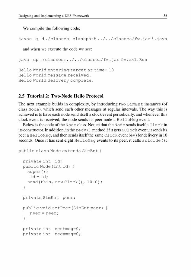
We compile the following code:
javac g d ./classes classpath ../../classes/fw.jar *.java
and when we execute the code we see:
java cp ./classes:../../classes/fw.jar fw.ex1.Run
Hello World entering target at time: 10
Hello World message received.
Hello World delivery complete.
2.5 Tutorial 2: Two-Node Hello Protocol
The next example builds in complexity, by introducing two SimEnt instances (of
class Node), which send each other messages at regular intervals. The way this is
achieved is to have each node send itself a clock event periodically, and whenever this
clock event is received, the node sends its peer node a HelloMsg event.
Below is the code of the Node class. Notice that the Node sends itself a Clock in
its constructor. In addition, in therecv()method, if it gets aClock event, it sends its
peer aHelloMsg, and then sends itself the sameClock event (ev) for delivery in 10
seconds. Once it has sent eight HelloMsg events to its peer, it calls suicide():
public class Node extends SimEnt {
private int id;
public Node(int id) {
super();
id = id;
send(this, new Clock(), 10.0);
}
private SimEnt peer;
public void setPeer(SimEnt peer) {
peer = peer;
}
private int sentmsg=0;
private int recvmsg=0;
Designing and Implementing a DES Framework 36

public void recv(SimEnt src, Event ev) {
if (ev instanceof Clock) {
send( peer, new HelloMsg(), 10.0);
sentmsg++;
if ( sentmsg<=8) send(this, ev, 10.0);
else this.suicide();
}
if (ev instanceof HelloMsg) {
recvmsg++;
System.out.println("Node"+ id+"recvmsg"+ recvmsg);
}
}
public String getName() {
return "Node";
}
public void deliveryAck(Scheduler.EventHandle h) { }
}
AlthoughNodewill receive an acknowledgement of the delivery of theHelloMsg
events through its deliveryAck() method, for simplicity we do not make it
respond to this notification.
Below is the HelloMsg event that is passed between Node instances:
public class HelloMsg implements Event {
public void entering(SimEnt locale) {}
}
Again, event though HelloMsg instances will be notified by the scheduler just
prior to being delivered to aSimEnt via theentering()method, for simplicitywe
do not make our HelloMsg react to these notification. Let us put the whole system
together now. The process is quite simple. We make two nodes, each informing the
other, then we start the scheduler:
public class Run {
public static void main(String [ ] args) {
Node n1 = new Node(1);
Node n2 = new Node(2);
37 Tutorial 2: Two Node Hello Protocol
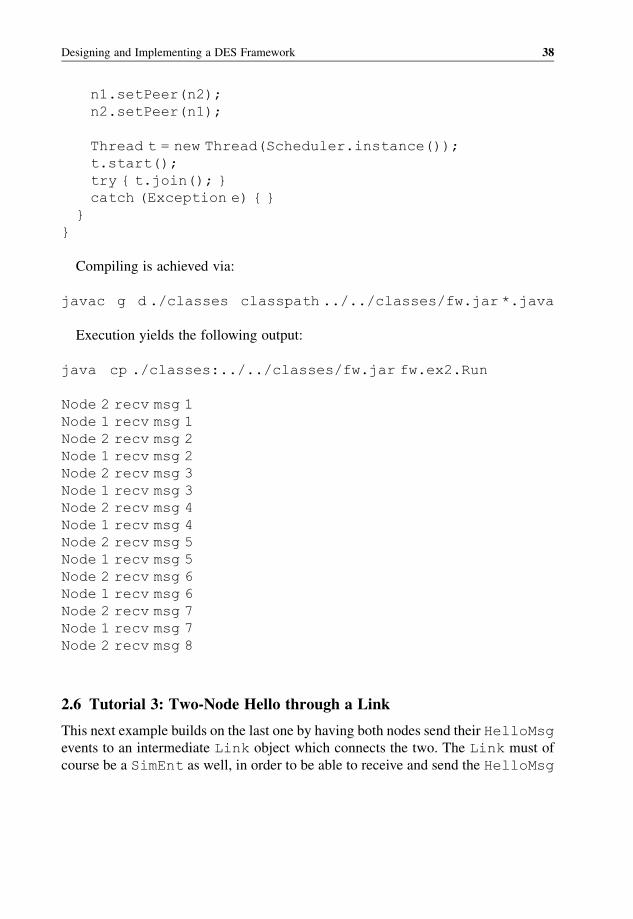
n1.setPeer(n2);
n2.setPeer(n1);
Thread t = new Thread(Scheduler.instance());
t.start();
try { t.join(); }
catch (Exception e) { }
}
}
Compiling is achieved via:
javac g d ./classes classpath ../../classes/fw.jar *.java
Execution yields the following output:
java cp ./classes:../../classes/fw.jar fw.ex2.Run
Node 2 recv msg 1
Node 1 recv msg 1
Node 2 recv msg 2
Node 1 recv msg 2
Node 2 recv msg 3
Node 1 recv msg 3
Node 2 recv msg 4
Node 1 recv msg 4
Node 2 recv msg 5
Node 1 recv msg 5
Node 2 recv msg 6
Node 1 recv msg 6
Node 2 recv msg 7
Node 1 recv msg 7
Node 2 recv msg 8
2.6 Tutorial 3: Two-Node Hello through a Link
This next example builds on the last one by having both nodes send their HelloMsg
events to an intermediate Link object which connects the two. The Link must of
course be a SimEnt as well, in order to be able to receive and send the HelloMsg
Designing and Implementing a DES Framework 38
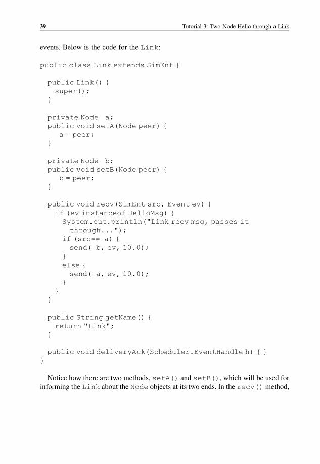
events. Below is the code for the Link:
public class Link extends SimEnt {
public Link() {
super();
}
private Node a;
public void setA(Node peer) {
a = peer;
}
private Node b;
public void setB(Node peer) {
b = peer;
}
public void recv(SimEnt src, Event ev) {
if (ev instanceof HelloMsg) {
System.out.println("Link recv msg, passes it
through...");
if (src== a) {
send( b, ev, 10.0);
}
else {
send( a, ev, 10.0);
}
}
}
public String getName() {
return "Link";
}
public void deliveryAck(Scheduler.EventHandle h) { }
}
Notice how there are two methods, setA() and setB(), which will be used for
informing the Link about the Node objects at its two ends. In the recv()method,
39 Tutorial 3: Two Node Hello through a Link
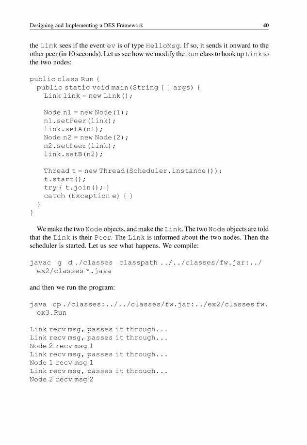
the Link sees if the event ev is of type HelloMsg. If so, it sends it onward to the
other peer (in 10 seconds). Let us see howwemodify theRun class to hook upLink to
the two nodes:
public class Run {
public static void main(String [ ] args) {
Link link = new Link();
Node n1 = new Node(1);
n1.setPeer(link);
link.setA(n1);
Node n2 = new Node(2);
n2.setPeer(link);
link.setB(n2);
Thread t = new Thread(Scheduler.instance());
t.start();
try { t.join(); }
catch (Exception e) { }
}
}
Wemake the twoNode objects, andmake theLink. The twoNode objects are told
that the Link is their Peer. The Link is informed about the two nodes. Then the
scheduler is started. Let us see what happens. We compile:
javac g d ./classes classpath ../../classes/fw.jar:../
ex2/classes *.java
and then we run the program:
java cp ./classes:../../classes/fw.jar:../ex2/classes fw.
ex3.Run
Link recv msg, passes it through...
Link recv msg, passes it through...
Node 2 recv msg 1
Link recv msg, passes it through...
Node 1 recv msg 1
Link recv msg, passes it through...
Node 2 recv msg 2
Designing and Implementing a DES Framework 40
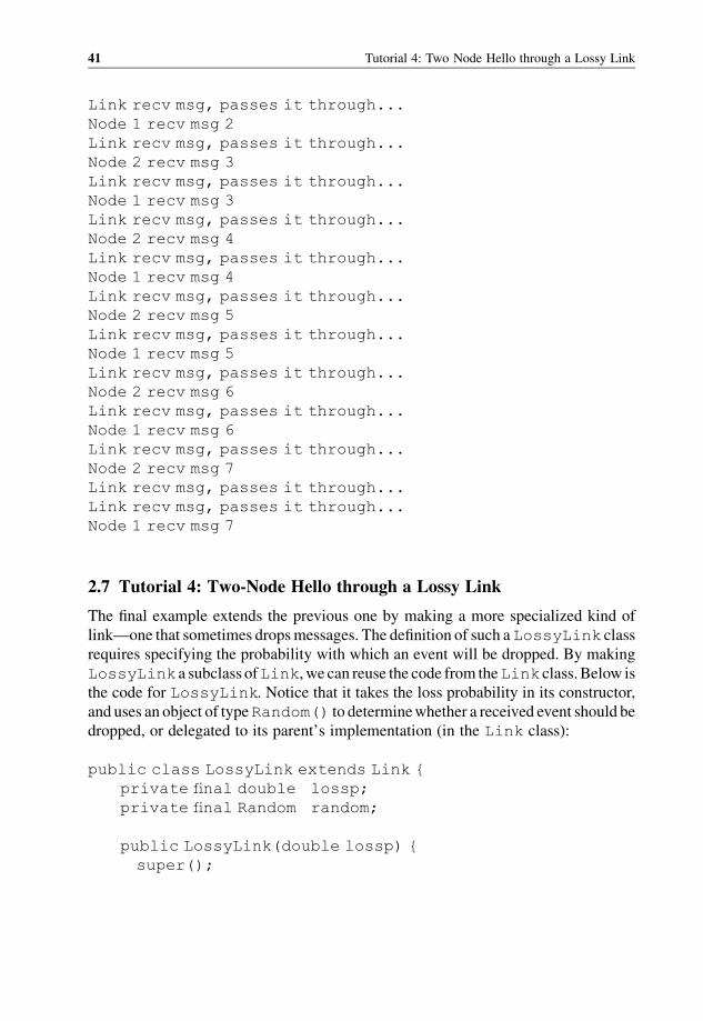
Link recv msg, passes it through...
Node 1 recv msg 2
Link recv msg, passes it through...
Node 2 recv msg 3
Link recv msg, passes it through...
Node 1 recv msg 3
Link recv msg, passes it through...
Node 2 recv msg 4
Link recv msg, passes it through...
Node 1 recv msg 4
Link recv msg, passes it through...
Node 2 recv msg 5
Link recv msg, passes it through...
Node 1 recv msg 5
Link recv msg, passes it through...
Node 2 recv msg 6
Link recv msg, passes it through...
Node 1 recv msg 6
Link recv msg, passes it through...
Node 2 recv msg 7
Link recv msg, passes it through...
Link recv msg, passes it through...
Node 1 recv msg 7
2.7 Tutorial 4: Two-Node Hello through a Lossy Link
The final example extends the previous one by making a more specialized kind of
link—one that sometimes dropsmessages. The definition of such aLossyLink class
requires specifying the probability with which an event will be dropped. By making
LossyLink a subclass ofLink, we can reuse the code from theLink class. Below is
the code for LossyLink. Notice that it takes the loss probability in its constructor,
and uses an object of typeRandom() to determinewhether a received event should be
dropped, or delegated to its parent’s implementation (in the Link class):
public class LossyLink extends Link {
private final double lossp;
private final Random random;
public LossyLink(double lossp) {
super();
41 Tutorial 4: Two Node Hello through a Lossy Link
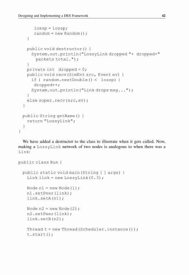
lossp = lossp;
random = new Random();
}
public void destructor() {
System.out.println("LossyLink dropped "+ dropped+"
packets total.");
}
private int dropped = 0;
public void recv(SimEnt src, Event ev) {
if ( random.nextDouble() < lossp) {
dropped++;
System.out.println("Link drops msg...");
}
else super.recv(src,ev);
}
public String getName() {
return "LossyLink";
}
}
We have added a destructor to the class to illustrate when it gets called. Now,
making a LossyLink network of two nodes is analogous to when there was a
Link:
public class Run {
public static void main(String [ ] args) {
Link link = new LossyLink(0.3);
Node n1 = new Node(1);
n1.setPeer(link);
link.setA(n1);
Node n2 = new Node(2);
n2.setPeer(link);
link.setB(n2);
Thread t = new Thread(Scheduler.instance());
t.start();
Designing and Implementing a DES Framework 42
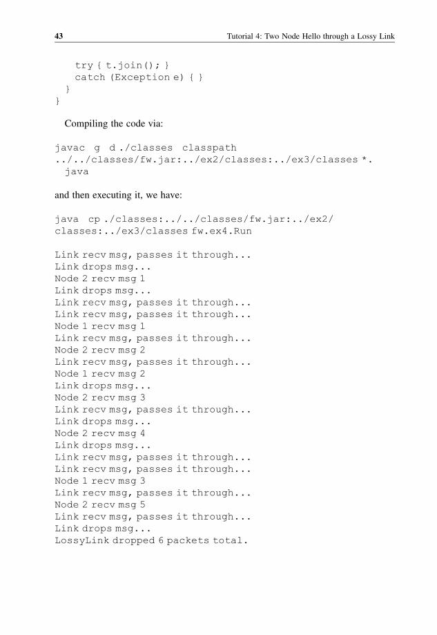
try { t.join(); }
catch (Exception e) { }
}
}
Compiling the code via:
javac g d ./classes classpath
../../classes/fw.jar:../ex2/classes:../ex3/classes *.
java
and then executing it, we have:
java cp ./classes:../../classes/fw.jar:../ex2/
classes:../ex3/classes fw.ex4.Run
Link recv msg, passes it through...
Link drops msg...
Node 2 recv msg 1
Link drops msg...
Link recv msg, passes it through...
Link recv msg, passes it through...
Node 1 recv msg 1
Link recv msg, passes it through...
Node 2 recv msg 2
Link recv msg, passes it through...
Node 1 recv msg 2
Link drops msg...
Node 2 recv msg 3
Link recv msg, passes it through...
Link drops msg...
Node 2 recv msg 4
Link drops msg...
Link recv msg, passes it through...
Link recv msg, passes it through...
Node 1 recv msg 3
Link recv msg, passes it through...
Node 2 recv msg 5
Link recv msg, passes it through...
Link drops msg...
LossyLink dropped 6 packets total.
43 Tutorial 4: Two Node Hello through a Lossy Link
2.8 Summary
In this chapter, we have designed three cooperating classes that together serve as a
reusable foundation for a wide range of simulation software to be developed in
subsequent chapters. The three classes were: the Scheduler, which manages the
discrete passage of time; the SimEnt, which is the base abstract entity within the
simulation; and the Event, which is a temporally defined occurrence at a SimEnt.
The framework we developed will be referred to in future chapters as the framework
for discrete-event simulation (FDES). The FDES is quite compact, requiring fewer
than 250 lines of code, but powerful in that it provides an organizational structure for
discrete simulations. In the next chapter, we will consider a large case study that
illustrates the power of the framework in real-world settings. In later chapters, the
frameworkwill be extended to support specialized constructs and primitives necessary
for network simulation.
Recommended Reading
[1] E. Gamma, R. Helm, R. Johnson, and J. Vlissides, Design Patterns: Elements of Object Oriented
Software, Addison Wesley, 1995.
[2] L. P. Deutsch, “Design reuse and frameworks in the Smalltalk 80 system,” in Software Reusability,
Volume II: Applications and Experience ( T. J. Biggerstaff and A. J. Perlis,eds.), Addison Wesley,
1989.
[3] R. E. Johnson andB. Foote, “Designing reusable classes,” Journal ofObject Oriented Programming,
vol. 1, pp. 22 35, June/July 1988.
Designing and Implementing a DES Framework 44
3
Honeypot Communities: A CaseStudy with the Discrete-EventSimulation Framework
In this chapter, we will design and develop a simulation of a system that will generate
malware antivirus signatures using anuntrustedmulti-domain community of honeypots.
Roughly speaking, the honeypot community will act as a “Petri dish” for worms. The
distribution of sensors within the Internet will ensure that this Petri dish is a microcosm
reflecting overall wormdemographics. On the other hand, the small size of the Petri dish
will accelerate infection percolation rates, allowing automated antidote generation to
become feasiblewell in advance ofwhen thewormdisables the ambient larger network.
The system described here is based on an earlier system that was developed by the
authors and described in [1]. Unlike that publication, however, which focused on
experimental results and their implications, here the exposition is simplified and
entirely focused on the design and implementation of the necessary simulation software
itself. The purpose is to provide the readerwith a real case study illustrating howbuilds a
simulation using the Discrete Event Simulation Framework that we designed and
implemented inChapter 2. Beforewe develop the simulation of the proposed honeypot-
based system, let us begin with some background, so that themotivation of the problem
to be solved is clear, and the design of the proposed solution is compelling.
3.1 Background
Since the 1990s, computer worms have attacked the electronic community with
alarming regularity. Prominent examples include Melissa (1999), Code Red (2001),
Slammer (2003), Blaster (2003), and Sasser (2004), to name just a few! While the
economic impact of theseworm attacks is believed to be in excess of billions of dollars,
Network Modeling and Simulation M. Guizani, A. Rayes, B. Khan and A. Al Fuqaha
� 2010 John Wiley & Sons, Ltd.

there is no sure antidote against newly emergent worms. As such, society as a whole
remains vulnerable to the dangers that malware poses. Network worms spread over
the Internet by accessing services with exploitable implementation flaws or
“vulnerabilities.” Newly infected hosts serve as a stepping stone, advancing the
infection and leading to thousands of vulnerable hosts becoming compromised in a
very short time. Since worms have historically been static in their propagation
strategies, an attack against a vulnerable host typically follows a predictable pattern
or signature. Modem intrusion detection systems (IDSs) use the latter, by matching the
ports and byte sequences of incoming traffic to a specific signature in order to identify
worm traffic as it arrives and prevent the vulnerable services from seeing virulent
packets. Examples of popular IDSs include Bro [2] and Snort.
While signatures-based IDSs are successful against threats that are known in
advance, they remain useless against new worms because well-designed network
worms can propagate much more quickly than signatures can be generated. Most
commercial solutions rely on hand-generated signatures, which is a labor-intensive
process that takes on the order of hours or days. In contrast, modemworms spread fast
(e.g., the Slammer [3] worm can double its number of infections every 8.5 seconds and
can infect more than 90% of vulnerable hosts within 10 minutes). A comprehensive
solution to theworm problemmust be able to detect newworms and rapidly provide an
active response without labor-intensive human interaction.
A number of approaches for detecting and responding to worms have been
considered. The idea of collaborative intrusion detection itself is not new. The
Worminator system uses alerts that are shared within a distributed IDS in order to
detect an attack in progress. The DOMINO system makes a strong case for collabora-
tive intrusion detection by demonstrating that blacklists can be constructed more
quickly using a large, distributed, collaborative system. However, the veracity of
shared information is difficult to verify in such schemes; as is usually the case,
participants are required to trust one another.
Detection systems use a passive network telescope [5]—blocks of previously
unallocated IP addresses—to capture scan traffic. Such detection allows only the
most crude form of response since all clients must be blocked from access to a
vulnerable service until it has been secured. Collaborative detectors of this form also
require total trust among all participants.
Content filtering systems attempt to stop infections at the destination. Signature
systems such as EarlyBird and Autograph [7] observe flows from infected machines,
identify blocks common across many of those flows, and dynamically create IDS
signatures to enable content filtering. In order to generate signatures, a source of
malicious flows is required. Autograph requires a large deployment to obtain
malicious flows rapidly. The Honeycomb [8] project collects malicious flows
through medium-interaction honeypots. Both systems require total trust among
participants.
Honeypot Communities: A Case Study with the Discrete Event Simulation Framework 46

3.2 System Architecture
There aremany challenges in developing a scalable and comprehensive solution that is
capable of thwarting worm propagation:
. The system must be able to detect worms early, before they become widespread.
. The systemmust be accurate: there should be no false negatives (noworms should go
undetected) and no false positives (since network messages misdiagnosed as worms
can cause denied service).. The system should automatically generate countermeasures that can be fully tested
and guaranteed to be effective in catching not only known worms, but also new
worms that may be engineered to evade or subvert the system.. The system must be practical, reliable, and easily deployed and maintained.
In addition to these challenges, a serious obstacle is adoption. Network worms are
fast enough to overrun any detector deployed in a single administrative domain, thus
making the case for a distributed, collaborative detector. Collaboration that requires a
high degree of trust among participants is unlikely to be deployed, hence our goal is:
Maximize coverage in the network, while minimizing trust requirements.
Our system works as follows: a set of sensor machines and honeypot machines are
deployed throughout thewide area. Sensors divert all unsolicited traffic by tunneling it to
oneormore honeypots. If awormsuccessfully infects a honeypot, itwill attempt tomake
outgoing infection attempts to propagate itself. The host honeypot, however, tunnels all
outgoing attacks toward other honeypots. Once many honeypots have been infected, a
signature can be developed, and the people administering these honeypots can learn of
the platformandservices affectedby thewormand the signaturesdeveloped.Our system
is designed to be transparently distributed across multiple networks, allowing partici-
pants everywhere to join. A machine can join the system by becoming a sensor or a
honeypot. In contrast to prior efforts, participants in this system share actual infections
(rather than just sharing information)which can be locally verified using honeypots. The
system maximizes participation by minimizing trust required among the participants.
We now describe the components and functions of the system in more detail.
Sensors are machines configured to send “Unwanted” traffic into a honeypot.
Unwanted traffic is taken to be any traffic that would otherwise be dropped by the
sensor. Examples include unsolicited connections (TCP SYN packets), UDP packets
to unused ports, incoming ICMP requests, and so on, all ofwhich are sent to a honeypot
by means of an SSL tunnel. Sensors are cheap since existing machines and firewalls at
the front of the network can be configured to route unwanted traffic for many IP
addresses to distinct honeypots.
47 System Architecture
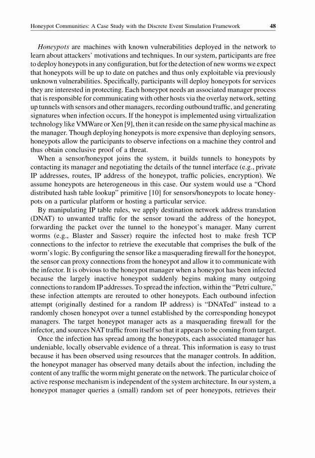
Honeypots are machines with known vulnerabilities deployed in the network to
learn about attackers’ motivations and techniques. In our system, participants are free
to deploy honeypots in any configuration, but for the detection of newwormswe expect
that honeypots will be up to date on patches and thus only exploitable via previously
unknown vulnerabilities. Specifically, participants will deploy honeypots for services
they are interested in protecting. Each honeypot needs an associated manager process
that is responsible for communicatingwith other hosts via the overlay network, setting
up tunnelswith sensors and othermanagers, recording outbound traffic, and generating
signatures when infection occurs. If the honeypot is implemented using virtualization
technology likeVMWare orXen [9], then it can reside on the same physicalmachine as
the manager. Though deploying honeypots is more expensive than deploying sensors,
honeypots allow the participants to observe infections on a machine they control and
thus obtain conclusive proof of a threat.
When a sensor/honeypot joins the system, it builds tunnels to honeypots by
contacting its manager and negotiating the details of the tunnel interface (e.g., private
IP addresses, routes, IP address of the honeypot, traffic policies, encryption). We
assume honeypots are heterogeneous in this case. Our system would use a “Chord
distributed hash table lookup” primitive [10] for sensors/honeypots to locate honey-
pots on a particular platform or hosting a particular service.
By manipulating IP table rules, we apply destination network address translation
(DNAT) to unwanted traffic for the sensor toward the address of the honeypot,
forwarding the packet over the tunnel to the honeypot’s manager. Many current
worms (e.g., Blaster and Sasser) require the infected host to make fresh TCP
connections to the infector to retrieve the executable that comprises the bulk of the
worm’s logic. By configuring the sensor like amasquerading firewall for the honeypot,
the sensor can proxy connections from the honeypot and allow it to communicatewith
the infector. It is obvious to the honeypot manager when a honeypot has been infected
because the largely inactive honeypot suddenly begins making many outgoing
connections to random IP addresses. To spread the infection, within the “Petri culture,”
these infection attempts are rerouted to other honeypots. Each outbound infection
attempt (originally destined for a random IP address) is “DNATed” instead to a
randomly chosen honeypot over a tunnel established by the corresponding honeypot
managers. The target honeypot manager acts as a masquerading firewall for the
infector, and sourcesNAT traffic from itself so that it appears to be coming from target.
Once the infection has spread among the honeypots, each associated manager has
undeniable, locally observable evidence of a threat. This information is easy to trust
because it has been observed using resources that the manager controls. In addition,
the honeypot manager has observed many details about the infection, including the
content of any traffic thewormmight generate on the network. The particular choice of
active response mechanism is independent of the system architecture. In our system, a
honeypot manager queries a (small) random set of peer honeypots, retrieves their
Honeypot Communities: A Case Study with the Discrete Event Simulation Framework 48
observed flows, and uses these to attempt generation of a signature. Even if some
participants are malicious, they cannot influence signature generation unless they are
in amajority. Once a signature has been generated, its effectiveness can be tested using
the live copy of theworm that has been captured. Thisminimizes trust requirements for
generated signatures. To deploy the signature, the honeypot manager simply needs to
augment the IDSs it controls.
3.3 Simulation Modeling
Wenowpresent a discrete-time event simulator tomeasure the efficacy of the culturing
approach to worm detection under various parameters. The simulation considers a
network consisting of S sensors, H honeypots, and O ordinary machines. Each sensor
(resp. honeypot) knows only a small set of FEED HP (PEER HP) honeypots. Each of
these S þ H þ O machines is “vulnerable” to the worm with a probability
PRM PROB VULNERABLE. Initially, a set of INITIAL POP worms is instantiated
on distinct randomly chosen machines. Every SCAN PERIOD seconds, each worm
hurls itself toward an IP address which is taken to be in the set of sensor/honeypot/
ordinary machines with probability (S þ H þ O)/232. If the source of the worm is a
honeypot or sensor, then tunneling is simulated by taking the destination to be a
randomly chosen honeypot. If the source of the worm is an ordinary machine, then the
destination is simply taken to be a random machine. Finally, if the destination of the
transmission happens to be both vulnerable and uninfected, a new copy of the worm is
instantiated there. While the parameters are adjustable in our simulation environment,
we fix them at realistic values for the experiment.
Let us begin by making a list of the various SimEnt classes:
. Machine (an infectable computer or network element)
. Honeypot (a special kind of Machine)
. Sensor (another special kind of Machine)
. Env (a network of Machines)
. Worm (the malicious software)
. Experimenter (the nexus of statistical information from the simulation).
The most crucial element in a SimEnt’s behavior is how it responds to incoming
events in itsrecv()method. Inwhat follows, we consider thismethod for each of the
above SimEnts.
3.3.1 Event Response in a Machine, Honeypot, and Sensors
Amachine responds to the receipt of infection events by determining if the infection
is successful and, if so, becoming infected. Determination of vulnerability is
49 Simulation Modeling
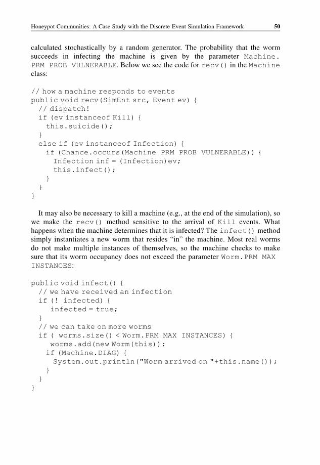
calculated stochastically by a random generator. The probability that the worm
succeeds in infecting the machine is given by the parameter Machine.
PRM PROB VULNERABLE. Below we see the code for recv() in the Machine
class:
// how a machine responds to events
public void recv(SimEnt src, Event ev) {
// dispatch!
if (ev instanceof Kill) {
this.suicide();
}
else if (ev instanceof Infection) {
if (Chance.occurs(Machine PRM PROB VULNERABLE)) {
Infection inf = (Infection)ev;
this.infect();
}
}
}
It may also be necessary to kill a machine (e.g., at the end of the simulation), so
we make the recv() method sensitive to the arrival of Kill events. What
happens when the machine determines that it is infected? The infect() method
simply instantiates a new worm that resides “in” the machine. Most real worms
do not make multiple instances of themselves, so the machine checks to make
sure that its worm occupancy does not exceed the parameter Worm.PRM MAX
INSTANCES:
public void infect() {
// we have received an infection
if (! infected) {
infected = true;
}
// we can take on more worms
if ( worms.size() < Worm.PRM MAX INSTANCES) {
worms.add(new Worm(this));
if (Machine.DIAG) {
System.out.println("Worm arrived on "+this.name());
}
}
}
Honeypot Communities: A Case Study with the Discrete Event Simulation Framework 50

3.3.2 Event Response in a Worm
Aworm is always made by a machine when it receives an Infection event (and
probabilistically determines that the infection was successful). At the time when the
worm is instantiated, it is told the identity of its host machine (or “residence”):
public Worm(Machine residence) {
super();
residence = residence;
TimeTick tt = new TimeTick(PRM WORM WAKEUP);
this.send(this, tt, tt.getPeriod());
}
A worm responds to TimeTick events by asking its host (machine, sensor, or
honeypot) for a random neighboring machine (“peer”). The worm then hurls itself at
this random neighbor using an Infection event. As above, it may be necessary to
kill a worm (e.g., at the end of the simulation), so we make the recv() method
sensitive to the arrival of Kill events:
public void recv(SimEnt src, Event ev) {
// dispatch!
if (ev instanceof Kill) {
this.suicide();
}
else if (ev instanceof TimeTick) {
TimeTick tt = (TimeTick)ev;
Machine h = residence.getRandomPeer();
if (h!=null) {
// diag
Infection inf = new Infection();
this.send(h, inf, 0.0);
residence.outboundTrafficNotification();
}
// register next tick
this.send(this, tt, tt.getPeriod());
}
}
Note that thegetRandomPeer()method that thewormuses to obtain the address
of its next victim is overloaded in the Sensor and Honeypot subclasses of
Machine. In this way, a machine provides a random network neighbor, while sensors
51 Simulation Modeling
always tunnel infections into honeypots, and honeypots always tunnel the infection
into other honeypots.
Here is getRandomPeer() in Machine:
public Machine getRandomPeer() {
if ( peerMachines.size() == 0) return null;
int index = (int)(Math.random()*(double) peerMachines.
size());
return (Machine) peerMachines.get(index);
}
Compare this with getRandomPeer() in Sensor:
public Machine getRandomPeer() {
// only allow outbound connections to Honeypots
if ( feedHoneypots.size() == 0) return null;
int index = (int)(Math.random()*(double) feedHoneypots.
size());
return (Honeypot) feedHoneypots.get(index);
}
and getRandomPeer() in Honeypot:
public Machine getRandomPeer() {
// only allow outbound connections to Honeypots
if ( peerHoneypots.size() == 0) return null;
int index = (int)(Math.random()*(double) peerHoneypots.
size());
return (Honeypot) peerHoneypots.get(index);
}
The worm also calls outboundTrafficNotification() on its residence to
allow the host to respond to its outward propagation attempt. Regular machines and
sensors do not respond in any way to this notification (their implementation of the
method is empty), but honeypots do. They attempt to construct a signature for the
worm. This happens successfully if the number of observed outbound propagations of
the worm exceeds PRM SIG MINSTREAMS:
void outboundTrafficNotification() {
// Does the traffic "slip past us"?
if (Chance.occurs(PRM PROB TRAFFIC OBSERVED)) {
Honeypot Communities: A Case Study with the Discrete Event Simulation Framework 52
// outbound traffic has been observed!
seentraffic = true;
int numStreams = 0;
int totalPeers = 0;
// begin Rabinizing...
for (Iterator it= peerHoneypots.iterator(); it.hasNext
();)
{
Honeypot h = (Honeypot)it.next();
if (h. seentraffic) numStreams++;
totalPeers++;
}
if (numStreams >= PRM SIG MINSTREAMS) {
// signature construction succeeds
antidote = true;
if (diagOn()) {
System.out.println("Antidote developed on "+this.
name());
}
if (PRM SELFISH HONEYPOT) {
// the admin takes the honeypot offline
this.suicide();
}
}
}
}
The simulation is made more sophisticated by introducing the possibility that the
worm may manage to transmit itself undetected (with probability PRM PROB
TRAFFIC OBSERVED). It is also possible that the administrator of the honeypot,
seeing that it is infected and has developed a signature, will take the honeypot offline
and refuse to share the antidote with others in the honeypot community.
3.3.3 System Initialization
Env is a singleton class:
private static Env instance;
public static Env instance() {
if ( instance == null) {
53 Simulation Modeling
instance = new Env();
}
return instance;
}
In its constructor, Env sends itself a Boot event:
private Env() {
super();
Boot b = new Boot();
this.send(this, b, 0.0);
}
Env is responsible for instantiating the network of machines, sensors, and honey-
pots, linking them up at the beginning of the simulation, and introducing the first
infection into the network:
public void recv(SimEnt src, Event ev) {
if (ev instanceof Boot) {
this.initialize();
// the initial infection!
Machine m = this.getRandomMachine();
System.out.println("# Initial infection on: "+m.name
());
m.infect();
}
}
public void initialize() {
// make machines
for (int i=0; i<PRM NUM MACHINES; i++) {
this.addMachine();
}
// make honeypots
for (int i=0; i<PRM NUM HONEYPOTS; i++) {
this.addHoneypot();
}
// make sensors
for (int i=0; i<PRM NUM SENSORS; i++) {
this.addSensor();
}
Honeypot Communities: A Case Study with the Discrete Event Simulation Framework 54
// link it up
this.linkMachines();
this.linkHoneypots();
this.linkSensors();
if (diagOn()) {
System.out.println("** Initial Environment **\n"+this.
toString());
}
}
Env maintains data structures for the machines, sensors, and honeypots:
private final LinkedList machines = new LinkedList();
private final LinkedList honeypots = new LinkedList();
private final LinkedList sensors = new LinkedList();
It supports methods to add to and remove from these data structures. These are used
in the implementation of the initialize() method:
public void addMachine() {
Machine m = new Machine();
machines.add(m);
}
public void addHoneypot() {
Honeypot h = new Honeypot();
honeypots.add(h);
}
public void addSensor() {
Sensor s = new Sensor();
sensors.add(s);
}
Env also provides methods to get random elements from these three categories:
public Machine getRandomMachine() {
if ( machines.size() == 0) return null;
int index = (int)(Math.random()*(double) machines.size());
return (Machine) machines.get(index);
55 Simulation Modeling
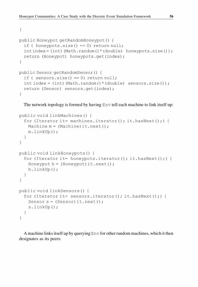
}
public Honeypot getRandomHoneypot() {
if ( honeypots.size() == 0) return null;
intindex=(int)(Math.random()*(double) honeypots.size());
return (Honeypot) honeypots.get(index);
}
public Sensor getRandomSensor() {
if ( sensors.size() == 0) return null;
int index = (int)(Math.random()*(double) sensors.size());
return (Sensor) sensors.get(index);
}
The network topology is formed by having Env tell each machine to link itself up:
public void linkMachines() {
for (Iterator it= machines.iterator(); it.hasNext();) {
Machine m = (Machine)it.next();
m.linkUp();
}
}
public void linkHoneypots() {
for (Iterator it= honeypots.iterator(); it.hasNext();) {
Honeypot h = (Honeypot)it.next();
h.linkUp();
}
}
public void linkSensors() {
for (Iterator it= sensors.iterator(); it.hasNext();) {
Sensor s = (Sensor)it.next();
s.linkUp();
}
}
Amachine links itself up by queryingEnv for other randommachines, which it then
designates as its peers:
Honeypot Communities: A Case Study with the Discrete Event Simulation Framework 56
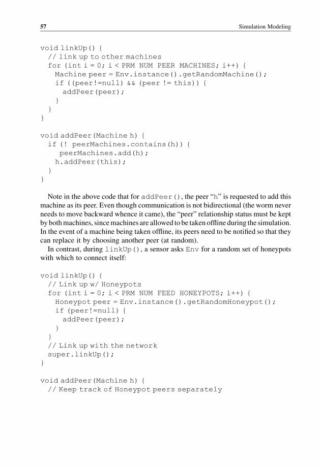
void linkUp() {
// link up to other machines
for (int i = 0; i < PRM NUM PEER MACHINES; i++) {
Machine peer = Env.instance().getRandomMachine();
if ((peer!=null) && (peer != this)) {
addPeer(peer);
}
}
}
void addPeer(Machine h) {
if (! peerMachines.contains(h)) {
peerMachines.add(h);
h.addPeer(this);
}
}
Note in the above code that for addPeer(), the peer “h” is requested to add this
machine as its peer. Even though communication is not bidirectional (the worm never
needs to move backward whence it came), the “peer” relationship status must be kept
by bothmachines, sincemachines are allowed to be taken offline during the simulation.
In the event of a machine being taken offline, its peers need to be notified so that they
can replace it by choosing another peer (at random).
In contrast, during linkUp(), a sensor asks Env for a random set of honeypots
with which to connect itself:
void linkUp() {
// Link up w/ Honeypots
for (int i = 0; i < PRM NUM FEED HONEYPOTS; i++) {
Honeypot peer = Env.instance().getRandomHoneypot();
if (peer!=null) {
addPeer(peer);
}
}
// Link up with the network
super.linkUp();
}
void addPeer(Machine h) {
// Keep track of Honeypot peers separately
57 Simulation Modeling

if (h instanceof Honeypot) {
if (! feedHoneypots.contains(h)) {
feedHoneypots.add(h);
h.addPeer(this);
}
}
else super.addPeer(h);
}
This is the similar towhat a honeypot doeswhen it is asked to undertakelinkUp():
void linkUp() {
// A Honeypot’s peers are only other Honeypots and
Sensors...
// Connect to Honeypots...
for (int i = 0; i < PRM NUM PEER HONEYPOTS; i++) {
Honeypot peer = Env.instance().getRandomHoneypot();
if ((peer!=null) && (peer != this)) {
addPeer(peer);
}
}
// The Sensors are responsible for linking to Honeypots...
// not the other way round, so we are done here...
}
void addPeer(Machine h) {
// A Honeypot’s peers are only other Honeypots or Sensors
if (h instanceof Honeypot) {
if (! peerHoneypots.contains(h)) {
peerHoneypots.add(h);
h.addPeer(this);
}
}
else if (h instanceof Sensor) {
if (! feedSensors.contains(h)) {
feedSensors.add(h);
h.addPeer(this);
}
}
}
Honeypot Communities: A Case Study with the Discrete Event Simulation Framework 58
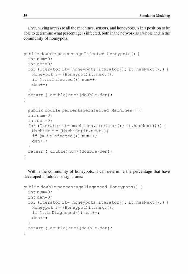
Env, having access to all themachines, sensors, and honeypots, is in a position to be
able to determinewhat percentage is infected, both in the network as awhole and in the
community of honeypots:
public double percentageInfected Honeypots() {
int num=0;
int den=0;
for (Iterator it= honeypots.iterator(); it.hasNext();) {
Honeypot h = (Honeypot)it.next();
if (h.isInfected()) num++;
den++;
}
return ((double)num/(double)den);
}
public double percentageInfected Machines() {
int num=0;
int den=0;
for (Iterator it= machines.iterator(); it.hasNext();) {
Machine m = (Machine)it.next();
if (m.isInfected()) num++;
den++;
}
return ((double)num/(double)den);
}
Within the community of honeypots, it can determine the percentage that have
developed antidotes or signatures:
public double percentageDiagnosed Honeypots() {
int num=0;
int den=0;
for (Iterator it= honeypots.iterator(); it.hasNext();) {
Honeypot h = (Honeypot)it.next();
if (h.isDiagnosed()) num++;
den++;
}
return ((double)num/(double)den);
}
59 Simulation Modeling
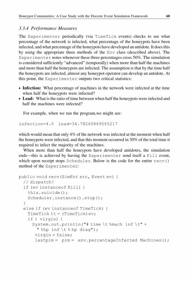
3.3.4 Performance Measures
The Experimenter periodically (via TimeTick events) checks to see what
percentage of the network is infected, what percentage of the honeypots have been
infected, andwhat percentage of the honeypots have developed an antidote. It does this
by using the appropriate three methods of the Env class (described above). The
Experimenter notes whenever these three percentages cross 50%. The simulation
is considered sufficiently “advanced” (temporally) when more than half the machines
and more than half the honeypots are infected. The assumption is that by the time half
the honeypots are infected, almost any honeypot operator can develop an antidote. At
this point, the Experimenter outputs two critical statistics:
. Infection: What percentage of machines in the network were infected at the time
when half the honeypots were infected?. Lead: What is the ratio of time between when half the honeypots were infected and
half the machines were infected?
For example, when we run the program,we might see:
infection=4.0 lead=34.78260869565217
which would mean that only 4% of the network was infected at the moment when half
the honeypots were infected, and that this moment occurred in 30% of the total time it
required to infect the majority of the machines.
When more than half the honeypots have developed antidotes, the simulation
ends—this is achieved by having the Experimenter send itself a Kill event,
which upon receipt stops Scheduler. Below is the code for the entire recv()
method of the Experimenter:
public void recv(SimEnt src, Event ev) {
// dispatch!
if (ev instanceof Kill) {
this.suicide();
Scheduler.instance().stop();
}
else if (ev instanceof TimeTick) {
TimeTick tt = (TimeTick)ev;
if ( virgin) {
System.out.println("# time \t %mach inf \t" +
" %hp inf \t % hp diag");
virgin = false;
lastpim = pim = env.percentageInfected Machines();
Honeypot Communities: A Case Study with the Discrete Event Simulation Framework 60
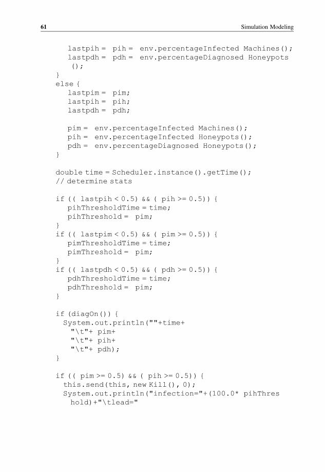
lastpih = pih = env.percentageInfected Machines();
lastpdh = pdh = env.percentageDiagnosed Honeypots
();
}
else {
lastpim = pim;
lastpih = pih;
lastpdh = pdh;
pim = env.percentageInfected Machines();
pih = env.percentageInfected Honeypots();
pdh = env.percentageDiagnosed Honeypots();
}
double time = Scheduler.instance().getTime();
// determine stats
if (( lastpih < 0.5) && ( pih >= 0.5)) {
pihThresholdTime = time;
pihThreshold = pim;
}
if (( lastpim < 0.5) && ( pim >= 0.5)) {
pimThresholdTime = time;
pimThreshold = pim;
}
if (( lastpdh < 0.5) && ( pdh >= 0.5)) {
pdhThresholdTime = time;
pdhThreshold = pim;
}
if (diagOn()) {
System.out.println(""+time+
"\t"+ pim+
"\t"+ pih+
"\t"+ pdh);
}
if (( pim >= 0.5) && ( pih >= 0.5)) {
this.send(this, new Kill(), 0);
System.out.println("infection="+(100.0* pihThres
hold)+"\tlead="
61 Simulation Modeling

(100.0* pihThresholdTime/ pimThresholdTime));
}
// register next tick
this.send(this, tt, tt.getPeriod());
}
}
3.3.5 System Parameters
In the course of defining the variousSimEnts, we havemade use ofmany parameters.
Let us catalog them now:
. Machine (an infectable computer or network element):
- PRM NUM PEER MACHINES
- PRM PROB VULNERABLE
. Honeypot (a special kind of Machine):
- PRM NUM PEER HONEYPOTS
- PRM PROB TRAFFIC OBSERVED
- PRM SIG MINSTREAMS
- PRM SELFISH HONEYPOT
. Sensor (another special kind of Machine):
- PRM SENSOR WAKEUP
- PRM PROB INFECTION
- PRM NUM FEED HONEYPOTS
. Env (a network of Machines):
- PRM NUM MACHINES
- PRM NUM HONEYPOTS
- PRM NUM SENSORS
. Worm (the malicious software):
- PRM MAX INSTANCES
- PRM WORM WAKEUP
Rather than have these parameters takevalues that are set in each of the individual class
source files, we can aggregate them all into a single class calledParam, so that there is
a centralized place where simulation parameters are defined:
// Environment
// number of honeypots
public static int Env PRM NUM HONEYPOTS = 8;
Honeypot Communities: A Case Study with the Discrete Event Simulation Framework 62
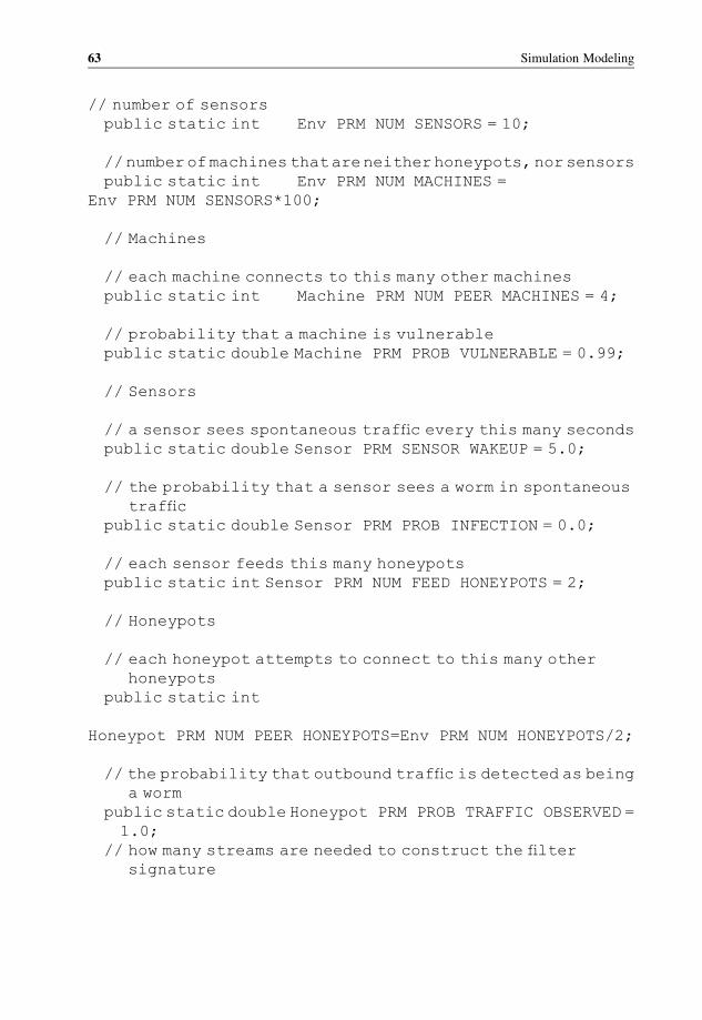
// number of sensors
public static int Env PRM NUM SENSORS = 10;
//numberofmachinesthatareneitherhoneypots,norsensors
public static int Env PRM NUM MACHINES =
Env PRM NUM SENSORS*100;
// Machines
// each machine connects to this many other machines
public static int Machine PRM NUM PEER MACHINES = 4;
// probability that a machine is vulnerable
public static double Machine PRM PROB VULNERABLE = 0.99;
// Sensors
// a sensor sees spontaneous traffic every this many seconds
public static double Sensor PRM SENSOR WAKEUP = 5.0;
// the probability that a sensor sees a worm in spontaneous
traffic
public static double Sensor PRM PROB INFECTION = 0.0;
// each sensor feeds this many honeypots
public static int Sensor PRM NUM FEED HONEYPOTS = 2;
// Honeypots
// each honeypot attempts to connect to this many other
honeypots
public static int
Honeypot PRM NUM PEER HONEYPOTS=Env PRM NUM HONEYPOTS/2;
// the probability that outbound traffic is detected as being
a worm
public static double Honeypot PRM PROB TRAFFIC OBSERVED =
1.0;
// how many streams are needed to construct the filter
signature
63 Simulation Modeling
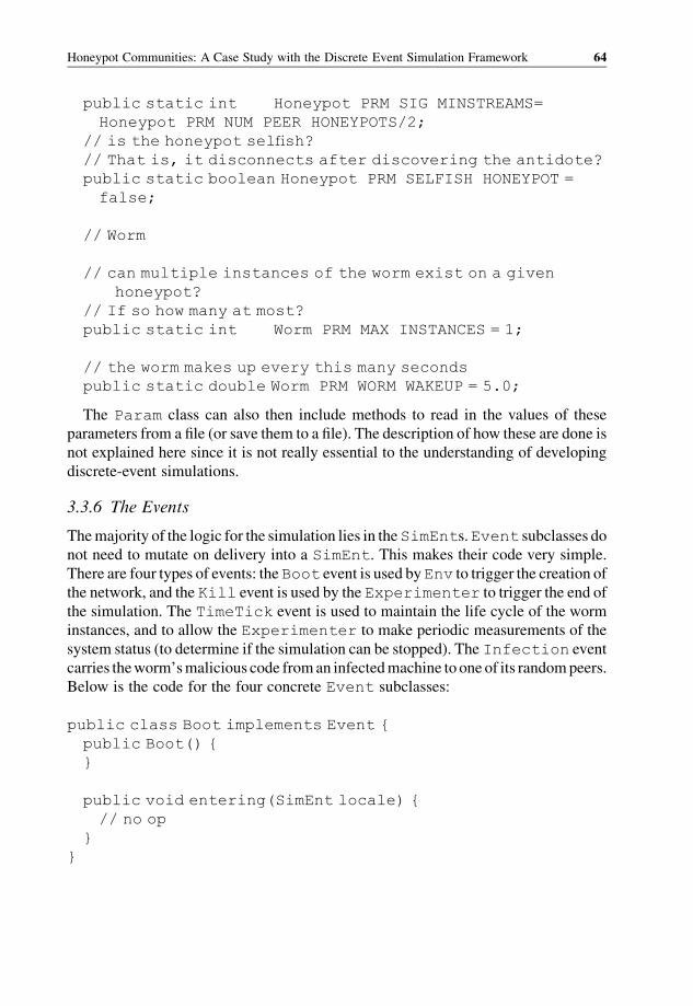
public static int Honeypot PRM SIG MINSTREAMS=
Honeypot PRM NUM PEER HONEYPOTS/2;
// is the honeypot selfish?
// That is, it disconnects after discovering the antidote?
public static boolean Honeypot PRM SELFISH HONEYPOT =
false;
// Worm
// can multiple instances of the worm exist on a given
honeypot?
// If so how many at most?
public static int Worm PRM MAX INSTANCES = 1;
// the worm makes up every this many seconds
public static double Worm PRM WORM WAKEUP = 5.0;
The Param class can also then include methods to read in the values of these
parameters from a file (or save them to a file). The description of how these are done is
not explained here since it is not really essential to the understanding of developing
discrete-event simulations.
3.3.6 The Events
Themajority of the logic for the simulation lies in theSimEnts.Event subclasses do
not need to mutate on delivery into a SimEnt. This makes their code very simple.
There are four types of events: theBoot event is used byEnv to trigger the creation of
the network, and the Kill event is used by the Experimenter to trigger the end of
the simulation. The TimeTick event is used to maintain the life cycle of the worm
instances, and to allow the Experimenter to make periodic measurements of the
system status (to determine if the simulation can be stopped). The Infection event
carries theworm’smalicious code froman infectedmachine to one of its randompeers.
Below is the code for the four concrete Event subclasses:
public class Boot implements Event {
public Boot() {
}
public void entering(SimEnt locale) {
// no op
}
}
Honeypot Communities: A Case Study with the Discrete Event Simulation Framework 64
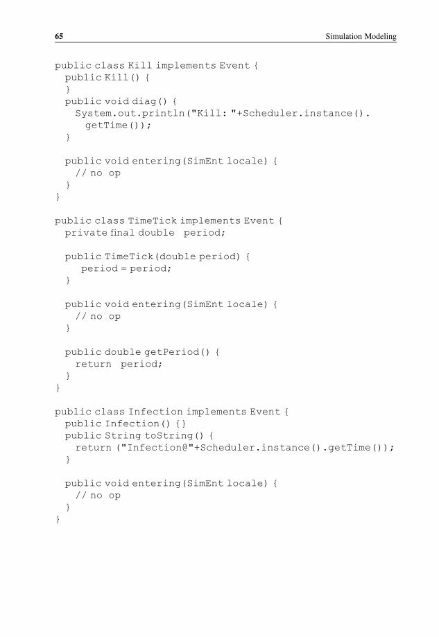
public class Kill implements Event {
public Kill() {
}
public void diag() {
System.out.println("Kill: "+Scheduler.instance().
getTime());
}
public void entering(SimEnt locale) {
// no op
}
}
public class TimeTick implements Event {
private final double period;
public TimeTick(double period) {
period = period;
}
public void entering(SimEnt locale) {
// no op
}
public double getPeriod() {
return period;
}
}
public class Infection implements Event {
public Infection() {}
public String toString() {
return ("Infection@"+Scheduler.instance().getTime());
}
public void entering(SimEnt locale) {
// no op
}
}
65 Simulation Modeling
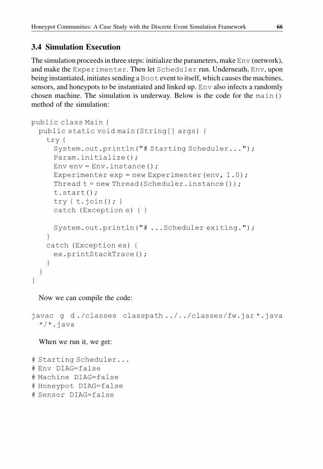
3.4 Simulation Execution
The simulation proceeds in three steps: initialize the parameters, makeEnv (network),
and make the Experimenter. Then let Scheduler run. Underneath, Env, upon
being instantiated, initiates sending aBoot event to itself, which causes themachines,
sensors, and honeypots to be instantiated and linked up. Env also infects a randomly
chosen machine. The simulation is underway. Below is the code for the main()
method of the simulation:
public class Main {
public static void main(String[] args) {
try {
System.out.println("# Starting Scheduler...");
Param.initialize();
Env env = Env.instance();
Experimenter exp = new Experimenter(env, 1.0);
Thread t = new Thread(Scheduler.instance());
t.start();
try { t.join(); }
catch (Exception e) { }
System.out.println("# ...Scheduler exiting.");
}
catch (Exception ex) {
ex.printStackTrace();
}
}
}
Now we can compile the code:
javac g d ./classes classpath ../../classes/fw.jar *.java
*/*.java
When we run it, we get:
# Starting Scheduler...
# Env DIAG=false
# Machine DIAG=false
# Honeypot DIAG=false
# Sensor DIAG=false
Honeypot Communities: A Case Study with the Discrete Event Simulation Framework 66
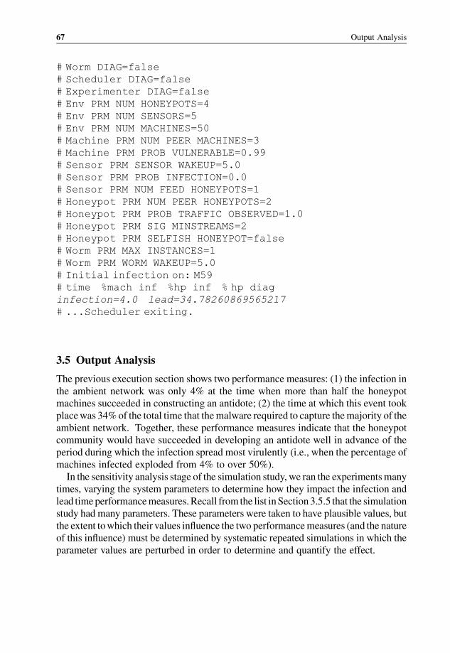
# Worm DIAG=false
# Scheduler DIAG=false
# Experimenter DIAG=false
# Env PRM NUM HONEYPOTS=4
# Env PRM NUM SENSORS=5
# Env PRM NUM MACHINES=50
# Machine PRM NUM PEER MACHINES=3
# Machine PRM PROB VULNERABLE=0.99
# Sensor PRM SENSOR WAKEUP=5.0
# Sensor PRM PROB INFECTION=0.0
# Sensor PRM NUM FEED HONEYPOTS=1
# Honeypot PRM NUM PEER HONEYPOTS=2
# Honeypot PRM PROB TRAFFIC OBSERVED=1.0
# Honeypot PRM SIG MINSTREAMS=2
# Honeypot PRM SELFISH HONEYPOT=false
# Worm PRM MAX INSTANCES=1
# Worm PRM WORM WAKEUP=5.0
# Initial infection on: M59
# time %mach inf %hp inf % hp diag
infection=4.0 lead=34.78260869565217
# ...Scheduler exiting.
3.5 Output Analysis
The previous execution section shows two performance measures: (1) the infection in
the ambient network was only 4% at the time when more than half the honeypot
machines succeeded in constructing an antidote; (2) the time at which this event took
placewas 34%of the total time that themalware required to capture themajority of the
ambient network. Together, these performance measures indicate that the honeypot
community would have succeeded in developing an antidote well in advance of the
period during which the infection spread most virulently (i.e., when the percentage of
machines infected exploded from 4% to over 50%).
In the sensitivity analysis stage of the simulation study, we ran the experimentsmany
times, varying the system parameters to determine how they impact the infection and
lead time performancemeasures.Recall from the list inSection3.5.5 that the simulation
study had many parameters. These parameters were taken to have plausible values, but
the extent towhich their values influence the two performancemeasures (and the nature
of this influence) must be determined by systematic repeated simulations in which the
parameter values are perturbed in order to determine and quantify the effect.
67 Output Analysis
3.6 Summary
We developed a discrete-event simulation of a honeypot community-based system for
automatic worm detection and immunization. The simulations showed that the
infection in the ambient network was lower than 5% at the time when most honeypot
machines were able to construct an antidote. This antidote construction became
possible early, in about one-third of the time required for the malware to infect the
majority of ambient networks. The simulations indicate that the proposed system
architecture is effective at antidote generation for emergent malware. This is just one
application of many where discrete-event simulation could be used. The reader could
extend this type to other network applications, such as P2P, sensor networks, ad hoc
networks, collaborative networks, cognitive radios, multimedia over wireless, as well
as Internet applications.
Recommended Reading
[1] J. Sandin and B. Khan, “Petrifying worm cultures: scalable detection and immunization in
untrusted environments,” Proceedings of IEEE International Conference on Communications
(ICC 2007), Glasgow, Scotland, IEEE, 2077, pp. 1423 1428.
[2] V. Paxson, “Bro: a system for detecting network intruders in real time,” Computer Networks, vol.
31, no. 23 24, pp. 2435 2463, 1999.
[3] D. Moore, V. Paxson, S. Savage, C. Shannon, S. Staniford, and N. Weaver, “Inside the slammer
worm,” IEEE Security and Privacy, vol. 1, no. 4, pp. 33 39, 2003.
[4] C. C. Zou, L. Gao, W. Gong, and D. Towsley, “Monitoring and early warning for internet
worms,” Proceedings of the 10th ACIv1 Conference on Computer and communications
security, ACM Press, 2003, pp. 190 199.
[5] C. C. Zou, W. Gong, and D. Towsley, “Worm propagation modeling and analysis under dynamic
quarantine defense,” Proceedings of ACM Workshop on Rapid Malcode, ACM Press, 2003, pp.
51 60.
[6] N.Weaver, S. Staniford, andV. Paxson, “Very fast containment of scanningworms,”Proceedings of
the 13th USENIX Security Symposium, USENIX Association, 2004.
[7] H. A. Kim and B. Karp, “Autograph: toward automated, distributed worm signature detection,”
Proceedings of the 13th USENIX Security Symposium, USENIX Association, 2004.
[8] C. Kreibich and J. Croweroft, “Honeycomb: creating intrusion detection signatures using
honeypots,” SIGCOMM Computer Communication Review, vol. 34, no. 1, pp. 51 56, 2004.
[9] B. Dragovic, K. Fraser, S. Hand, T. Harris, A. Ho, I. Pratt, A. Warfield, P. Barham, and R.
Neugebauer, “Xen and the art of virtualization,” Proceedings of the ACM Symposium on
Operating Systems Principles, ACM, 2003.
[10] I. Stoica, R. Morris, D. Karger, F. Kaashoek, and H. Balakrishnan, “Chord: a scalable peer to peer
lookup service for internet applications,” Proceedings of ACM SIGCOMM, ACM, 2001, pp.
149 160.
Honeypot Communities: A Case Study with the Discrete Event Simulation Framework 68
4
Monte Carlo Simulation
Monte Carlo is a classical simulation technique. In fact, Monte Carlo is only one
particular application of an otherwise general method, which is applicable in both
deterministic and probabilistic settings. At the heart ofMonte Carlo is a computational
procedure in which a performance measure is estimated using samples drawn
randomly from a population with appropriate statistical properties. The selection of
samples, in turn, requires an appropriate randomnumber generator (RNG). Ideally, the
generated “random” sequences are a completely faithful software counterpart of the
non-determinism underlying the actual process.
The term Monte Carlo method is generally used to refer to any simulation
techniques related to the use of random numbers. This includes methods such as
Monte Carlo simulation, Monte Carlo integration, importance sampling, genetic
algorithms, simulated annealing, the Hasting–Metropolis algorithm, percolation,
random walk, and ballistic deposition, just to name a few. Of these, Monte Carlo
simulation is perhaps the most common and well-understood class of numerical
methods for computer simulations and experiments.MonteCarlo simulation generates
random inputs (in reference to a known distribution) and uses the inputs to determine a
numerical value of performance measure.
The essential part of the Monte Carlo simulation is a procedure for generating a
pseudo random number R that is distributed uniformly over the interval 0<R< 1.
Such a procedure is applied repeatedly within theMonte Carlo simulation to produce a
sequence of independently generated random numbers.
4.1 Characteristics of Monte Carlo Simulations
The input of the simulation is a distribution (based on some theoreticalmodel of reality,
or one built empirically from observations) over the set of inputs. Based on this
Network Modeling and Simulation M. Guizani, A. Rayes, B. Khan and A. Al Fuqaha
� 2010 John Wiley & Sons, Ltd.
distribution, theMonte Carlo simulation samples an instance of the inputs and runs the
simulation for this specific instance. The previous step of selecting inputs and running
the simulation is performed many times, and the results of these multiple simulations
are then aggregated in a numerically meaningful manner. The three features common
to all Monte Carlo simulations are:
1. A known distribution over the set of system inputs.
2. Random sampling of inputs based on the distribution specified in feature 1, and
simulation of the system under the selected inputs.
3. Numerical aggregation of experimental data collected from multiple simulations
conducted according to feature 2.
Numerical experiments of Monte Carlo simulation lead us to run the simulation on
many sampled inputs before we can infer the values of the system performance
measures of interest.
4.2 The Monte Carlo Algorithm
The Monte Carlo algorithm is based on the so-called law of large numbers. This
mathematical result of probability theory asserts that if one generates a large
numberN of samples x1, x2, . . . , xN from a space X, and compute a function f of each
of the samples, f(x1), f(x2), . . . , f(xN), then the mean of these values will approxi-
mate the mean value of f on the set X. That is, as N tends to |X|, we see that the
following holds:
ð1=NÞ½f ðx1Þþ f ðx2Þþ � � � þ f ðxNÞ� � f*ðXÞ the mean value of f on the elements of X:
4.2.1 A Toy Example: Estimating Areas
To further understand Monte Carlo simulation, let us examine a simple problem.
Below is a rectangle for which we know the length (10 units) and height (4 units). It is
split into two sections which are identified using different colors. What is the area
covered by the dark area?
Due to the irregular way in which the rectangle is split, this problem is not easily
solved using analytical methods. However, we can use Monte Carlo simulation to
easily find an approximate answer. The procedure is as follows:
1. Randomly select a location within the rectangle.
2. If it is within the dark area, record this instance as a hit.
3. Generate a new location and repeat 10 000 times.
Monte Carlo Simulation 70

After using Monte Carlo simulation to test 10 000 random scenarios, we will have a
pretty good average of how often the randomly selected location falls within the dark
area.
We also know from basic mathematics that the area of the rectangle is 40 square
units (length� height). Thus, the dark area can now be calculated by:
Dark area ¼ number of hits
10 000 scenarios� 40 square units:
Naturally, the number of random scenarios used by theMonteCarlo simulation does
not have to be 10 000. Ifmore scenarios are used, an evenmore accurate approximation
for the dark area can be obtained.
This almost toy-like example illustrates all the core ideas of Monte Carlo simula-
tion. As we move to a more complicated example, that of a charging car station, the
concepts we have seen will carry over:
. The notion of choosing a two-dimensional (2-D) point at randomwill generalize to a
higher-dimensional analog, e.g., choosing a sequence of electric car arrivals.. The question of whether the randomly chosen point is black or white will generalize
from a binary measurement to a continuous measurement, e.g., for each “point” the
percentage of time that the attendant of the charging station for electric cars was
busy.. The question of wanting to estimate the area of the black region generalizes to the
question of wanting to estimate the average value of the continuous measurement
(the average percentage of time that the attendant was busy) across all possible
sequences of electric car arrivals. Just as in the toy example above, this cannot be
easily determined precisely since we cannot possibly try all possible sequences of
electric car arrivals. Fortunately, however, as in the toy example, Monte Carlo
simulation lets us estimate this value.
Height = 4 Units
Length = 10 Units
What is the area under the curve (covered by the dark area)?
Figure 4.1 Distribution comparison
71 The Monte Carlo Algorithm

4.2.2 The Example of the Electric Car Battery Charging Station
Let us reconsider the charging station example from Section 1.3.1 of Chapter 1 where
we were interested in several performance measures, including:
. f: the maximum size of Q over the simulation’s duration; and
. g: the average percentage of time the server is busy.
By design, the simulation had several system parameters, including:
. D (governs electric car inter-creation intervals);
. F (governs the battery capacity); and
. M (the maximum battery charging rate).
We noted that even for fixed values of the system parameters D, F, and M, the
performance measures depend heavily on random choices made in the course of
the simulation. Thus, the system is non-deterministic and the performance measures
are themselves random variables. This is precisely a setting in which Monte Carlo
simulation could beapplied.Weassume thatD,F, andM arefixed (by consulting domain
experts or by mining real-world trace data from operating charging stations), then we
considerX to be the space of all possible electric car arrival histories, for which temporal
sequencing isgovernedby thedistribution implicit inD (andbattery capacity is governed
by the distribution implicit in F). The act of sampling x1 fromX amounts to specifying a
single electric car arrival history. For example, the arrival history x1 might be:
Electric car 1 arrived at time 1.0 having a battery capacity 10 kW that was 10% full.
Electric car 2 arrived at time 2.5 having a battery capacity 14 kW that was 80% full.
Electric car 3 arrived at time 5.5 having a battery capacity 3 kW that was 25% full.
Electric car 4 arrived at time 12.1 having a battery capacity 22 kW that was 5% full.
Now, given this sample, the system’s inputs are fully specified. We can run the
simulation and determine f(x1) and g(x1). The precise values of these performance
measures are highly dependent on the system parameters—in this case, the most
influential parameter is M (the other parameters D and F influence the electric car
arrival history). For some values of M, we might for example find that the maximum
queue size f(x1)¼ 2 and that the server was busy g(x1)¼ 75%of the time. Now,we can
select another electric car arrival history x2 from the space X. For example, the electric
car arrival history x2 might be:
Electric car 1 arrived at time 1.0 having a battery capacity 8 kW that was 20% full.
Electric car 2 arrived at time 2.0 having a battery capacity 18 kW that was 60% full.
Monte Carlo Simulation 72
Electric car 3 arrived at time 4.5 having a battery capacity 30 kW that was 45% full.
Electric car 4 arrived at time 8.7 having a battery capacity 2 kW that was 95% full.
As before, we can run the simulation and determine f(x2) and g(x2). The
procedure is repeated in this manner for a large number of sampled inputs N.
Each of the inputs x1, x2, . . . , xN is being sampled (i.e., chosen) according to known
and agreed-upon “distributions” that govern how likely each of the inputs (i.e.,
electric car arrival histories) is in practice. In all but the simplest cases, not all the xiare deemed to be equally likely—indeed if they are, the system may be amenable to
analytical modeling. Most computer programming languages or spreadsheets have
built-in functions to generate uniform distribution random numbers that can be
easily used. For example, one can use the RAND() function in Microsoft Excel or
RND in Visual Basic to generate random numbers between 0 and 1. One technical
hurdle that must be addressed when implementing a Monte Carlo simulation is how
one can generate other arbitrary (but specified) distributions using only the ability
to generate random numbers uniformly distributed between 0 and 1. Typically, this
feature is provided in most simulation frameworks, via the so-called inverse CDF
method.
Having collected a large number of performance measures for the sampled inputs
f(x1), f(x2), f(x3), . . . , f(xN) and g(x1), g(x2), g(x3), . . . , g(xN), we invoke the law of
large numbers to assert that the quantity:
ð1=NÞ½f ðx1Þþ f ðx2Þþ � � � þ f ðxNÞ�approaches f �(X), the mean value of f on the elements of X; and the quantity:
ð1=NÞ½gðx1Þþ gðx2Þþ � � � þ gðxNÞ�approaches g�(X), themeanvalue of g on the elements ofX. How largeN needs to be for
the “approach” to be close enough is often a difficult question to answer. We will see
how to incorporate determining N’s value in the course of the simulation itself.
Informally, the simulationwill repeatedly sample the nextxi fromX, compute f(xi) and
g(xi), and then ask “have we generated enough samples to be sure our estimate of the
performance is good?” Exactly this will be implemented computationally and will be
illustrated when we implement the electric car charging station example, using our
discrete-event simulation framework developed and discussed in Chapter 2.
4.2.3 Optimizing the Electric Car Battery Charging Station
Now, let us formulate an optimization problem for this system of the electric car
charging station. Suppose we find through surveys that customers would be willing to
73 The Monte Carlo Algorithm
join a line of four electric cars—but if the line at the station is five or more electric cars
in length, then customers would rather look for a different charging station. Manage-
ment is then very motivated to make sure that there are never more than four electric
cars in line. Suppose the electric charger manufacturer can provide chargers with
arbitrary high charging rates, but chargers with high charging rate cost more because
insurance costs are higher due to the likelihood of accidents. Suppose that a charger
with a charging rate of M kW per minute would cost the charging station’s owner
$1000M2. We know that D governs the electric car inter-creation intervals and F
governs battery capacity. Tominimize costs andmaximize profits,we seek the smallest
value ofM (charging rate) for which the maximum queue size exhibited by the system
is four or lower. How could this magical value of M be determined?
The essence of the approach is to set M to some number m1, run the Monte Carlo
simulation to determine the performancemeasure f �(X) given thatwe have setM¼m1.
Since we intend to vary the value ofMwewill write f �(X;m1) in place of f�(X) so that
the notation reminds us that this is the value of f when M¼m1. Now, intuitively, we
know that as the value ofM is increased, f �(X) will decrease, since electric cars can beserviced very quickly. We will increase M incrementally until we see that f �(X) hasdropped to a value that is at or below4. If we seek theminimal value ofM forwhich this
is true, then we will have to perform a binary search onM to find the precise value at
which f �(X) crosses 4.
4.3 Merits and Drawbacks
The main advantages of using a Monte Carlo simulation are:
. It provides approximate solutions to many mathematical problems concerning
systems that involve an element of randomness that can be modeled via a
distribution.. It also provides a framework for statistical sampling of inputs, allowing results from
numerical experiments to be aggregated in a meaningful way.. Its use is quite simple and straightforward as long as convergence can be guaranteed
by the theory.. For optimization problems, it often can reach global optima and overcome local
extrema.
A Monte Carlo simulation has the following limitations:
. It was originally developed to study properties of stable systems that are in
equilibrium—systems for which the values of performance measures are not
fluctuating. This means that X must be constructed in such a way that each sample
Monte Carlo Simulation 74
xi determines a system in steady state. In our previous exposition, we tookX to be the
set of arrival sequences for four electric cars. However, a charging station is probably
not in a “steady state” upon handling a sequence of four electric cars; its performance
measures f and gwill not have stabilized. It is more likely to be in a steady state (i.e.,
its performance measures f and g would have stabilized) when it has seen a large
number of electric cars, perhaps 40 000.Wewill see how to deal with the system if it
is in steady state and how to incorporate that into the simulation itself. Informally, the
simulation will construct samples from X and assess whether the sample describes a
system in steady state or not. If it is a sample of length 4, the answer will probably be
no, in which case it will be extended as needed. This will continue until eventually,
when it is a sample of 40 000 electric car arrivals, the simulation will determine that
the system defined by the sample is indeed in steady state. How exactly this is
implemented computationally will be illustrated when we implement the charging
station as a simulation, using the discrete-event simulation framework developed in
Chapter 2.. It is not universally agreedwhether thismethod can also be used to simulate a system
that is not in equilibrium (i.e., in a transient state).. To use a Monte Carlo simulation, one needs to generate a large number of input
samples—since before doing so, the law of large numbers need not to hold. This can
be time consuming in practice if each simulation itself takes a long time.. The results of a Monte Carlo simulation are only an approximation of the true
values.. When the performancemeasure has a high variance, the values produced by aMonte
Carlo simulation will converge to the mean value over X, but any given sample from
X may vary greatly from the computed mean.. The distribution over the set of inputs must be known in order to sample from X.
4.4 Monte Carlo Simulation for the Electric Car Charging Station
In this sectionwewill design and implement aMonteCarlo simulation for our example
of an electric car charging station, using the discrete-event simulation framework
developed in Chapter 2.
The entities in the simulation are:
. TrafficGen
. ChargingStation
. Server
Let us design and implement each of these in turn.
75 Monte Carlo Simulation for the Electric Car Charging Station
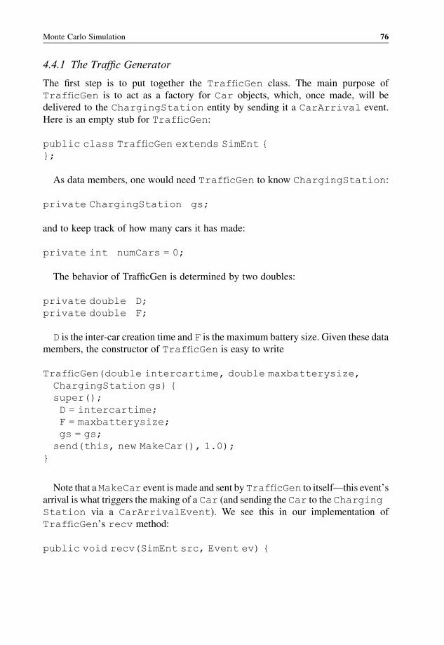
4.4.1 The Traffic Generator
The first step is to put together the TrafficGen class. The main purpose of
TrafficGen is to act as a factory for Car objects, which, once made, will be
delivered to the ChargingStation entity by sending it a CarArrival event.
Here is an empty stub for TrafficGen:
public class TrafficGen extends SimEnt {
};
As data members, one would need TrafficGen to know ChargingStation:
private ChargingStation gs;
and to keep track of how many cars it has made:
private int numCars = 0;
The behavior of TrafficGen is determined by two doubles:
private double D;
private double F;
D is the inter-car creation time and F is the maximum battery size. Given these data
members, the constructor of TrafficGen is easy to write
TrafficGen(double intercartime, double maxbatterysize,
ChargingStation gs) {
super();
D = intercartime;
F = maxbatterysize;
gs = gs;
send(this, new MakeCar(), 1.0);
}
Note that a MakeCar event is made and sent byTrafficGen to itself—this event’s
arrival is what triggers the making of a Car (and sending the Car to the Charging
Station via a CarArrivalEvent). We see this in our implementation of
TrafficGen’s recv method:
public void recv(SimEnt src, Event ev) {
Monte Carlo Simulation 76
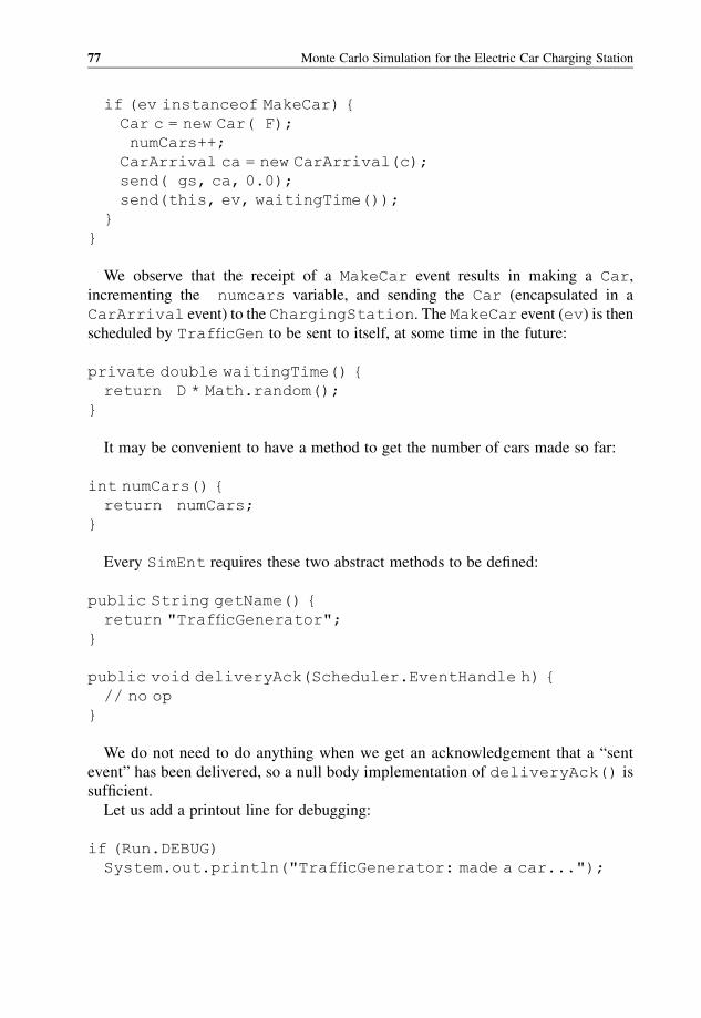
if (ev instanceof MakeCar) {
Car c = new Car( F);
numCars++;
CarArrival ca = new CarArrival(c);
send( gs, ca, 0.0);
send(this, ev, waitingTime());
}
}
We observe that the receipt of a MakeCar event results in making a Car,
incrementing the numcars variable, and sending the Car (encapsulated in a
CarArrival event) to the ChargingStation. The MakeCar event (ev) is then
scheduled by TrafficGen to be sent to itself, at some time in the future:
private double waitingTime() {
return D * Math.random();
}
It may be convenient to have a method to get the number of cars made so far:
int numCars() {
return numCars;
}
Every SimEnt requires these two abstract methods to be defined:
public String getName() {
return "TrafficGenerator";
}
public void deliveryAck(Scheduler.EventHandle h) {
// no op
}
We do not need to do anything when we get an acknowledgement that a “sent
event” has been delivered, so a null body implementation of deliveryAck() is
sufficient.
Let us add a printout line for debugging:
if (Run.DEBUG)
System.out.println("TrafficGenerator: made a car...");
77 Monte Carlo Simulation for the Electric Car Charging Station

For performance measurements to detect when steady state is achieved, we modify
TrafficGen by adding to the constructor:
Run.resetPercPerformanceMeasureStats();
then, inside the recv() method, when TrafficGen makes a car, it does the
following:
Run.calculatePercPerformanceMeasure();
if ( numCars % 100 == 0) {
if (! Run.terminatingBecausePercMeasureConverged()) {
Run.resetPercPerformanceMeasureStats();
}
else {
Scheduler.instance().stop();
}
}
The code fragment above calculates the performance measures and once the variables
have stabilized, the system is deemed to have reached a steady state. The operation of
the TrafficGen class requires two types of events: MakeCar and CarArrival.
These are relatively straightforward in their implementation:
public class MakeCar implements Event {
public void entering(SimEnt locale) {
// no op
}
}
public class CarArrival implements Event {
Car car;
CarArrival(Car c) {
car = c;
}
public void entering(SimEnt locale) {
// no op
}
}
Monte Carlo Simulation 78
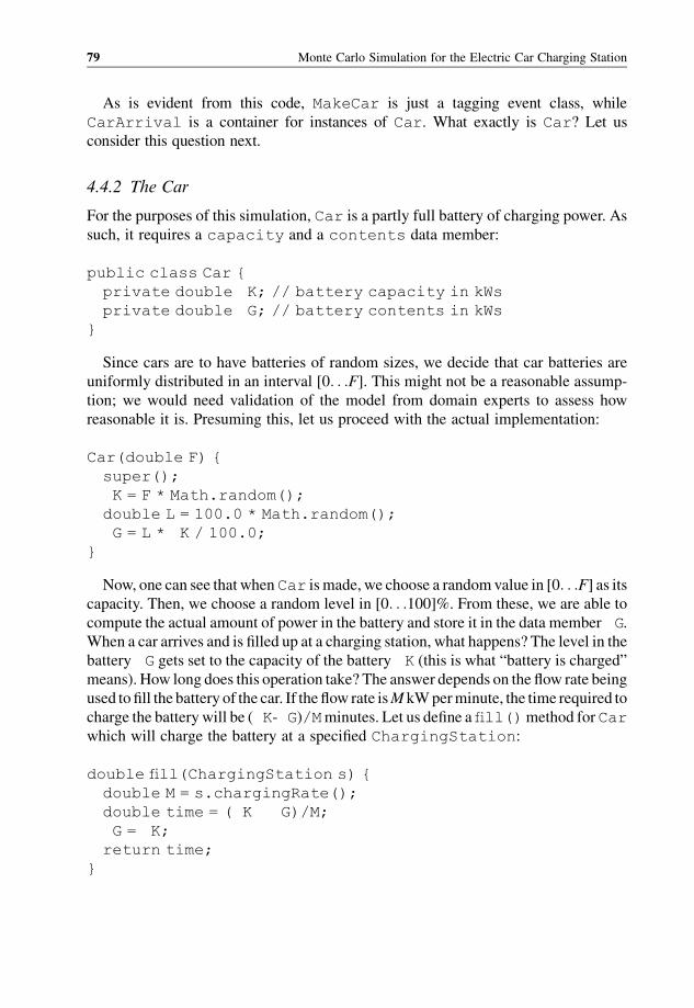
As is evident from this code, MakeCar is just a tagging event class, while
CarArrival is a container for instances of Car. What exactly is Car? Let us
consider this question next.
4.4.2 The Car
For the purposes of this simulation, Car is a partly full battery of charging power. As
such, it requires a capacity and a contents data member:
public class Car {
private double K; // battery capacity in kWs
private double G; // battery contents in kWs
}
Since cars are to have batteries of random sizes, we decide that car batteries are
uniformly distributed in an interval [0. . .F]. This might not be a reasonable assump-
tion; we would need validation of the model from domain experts to assess how
reasonable it is. Presuming this, let us proceed with the actual implementation:
Car(double F) {
super();
K = F * Math.random();
double L = 100.0 * Math.random();
G = L * K / 100.0;
}
Now, one can see that whenCar is made, we choose a randomvalue in [0. . .F] as itscapacity. Then, we choose a random level in [0. . .100]%. From these, we are able to
compute the actual amount of power in the battery and store it in the data member G.
When a car arrives and is filled up at a charging station, what happens? The level in the
battery G gets set to the capacity of the battery K (this is what “battery is charged”
means). How long does this operation take? The answer depends on the flow rate being
used to fill the battery of the car. If the flow rate isMkWperminute, the time required to
charge the battery will be ( K- G)/Mminutes. Let us define afill()method forCar
which will charge the battery at a specified ChargingStation:
double fill(ChargingStation s) {
double M = s.chargingRate();
double time = ( K G)/M;
G = K;
return time;
}
79 Monte Carlo Simulation for the Electric Car Charging Station
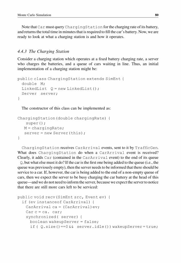
Note thatCarmust queryChargingStation for the charging rate of its battery,
and returns the total time inminutes that is required to fill the car’s battery. Now,we are
ready to look at what a charging station is and how it operates.
4.4.3 The Charging Station
Consider a charging station which operates at a fixed battery charging rate, a server
who charges the batteries, and a queue of cars waiting in line. Thus, an initial
implementation of a charging station might be:
public class ChargingStation extends SimEnt {
double M;
LinkedList Q = new LinkedList();
Server server;
}
The constructor of this class can be implemented as:
ChargingStation(double chargingRate) {
super();
M = chargingRate;
server = new Server(this);
}
ChargingStation receives CarArrival events, sent to it by TrafficGen.
What does ChargingStation do when a CarArrival event is received?
Clearly, it adds Car (contained in the CarArrival event) to the end of its queue
Q, but what elsemust it do? If the car is the first one being added to the queue (i.e., the
queuewas previously empty), then the server needs to be informed that there should be
service to a car. If, however, the car is being added to the end of a non-empty queue of
cars, then we expect the server to be busy charging the car battery at the head of this
queue—andwe do not need to inform the server, becausewe expect the server to notice
that there are still more cars left to be serviced:
public void recv(SimEnt src, Event ev) {
if (ev instanceof CarArrival) {
CarArrival ca = (CarArrival)ev;
Car c = ca. car;
synchronized( server) {
boolean wakeupServer = false;
if( Q.size()==0&& server.idle())wakeupServer=true;
Monte Carlo Simulation 80
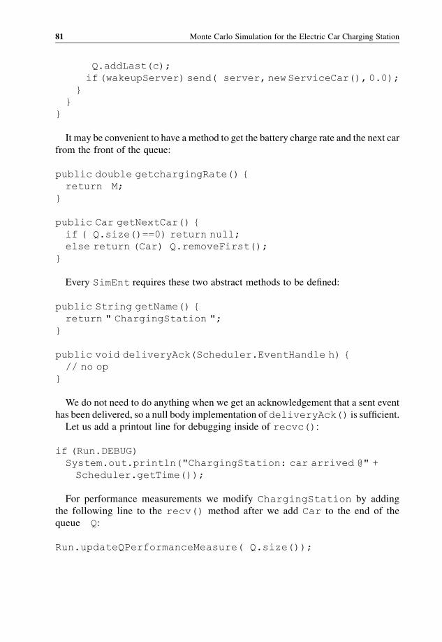
Q.addLast(c);
if(wakeupServer) send( server,newServiceCar(),0.0);
}
}
}
It may be convenient to have a method to get the battery charge rate and the next car
from the front of the queue:
public double getchargingRate() {
return M;
}
public Car getNextCar() {
if ( Q.size()==0) return null;
else return (Car) Q.removeFirst();
}
Every SimEnt requires these two abstract methods to be defined:
public String getName() {
return " ChargingStation ";
}
public void deliveryAck(Scheduler.EventHandle h) {
// no op
}
We do not need to do anything when we get an acknowledgement that a sent event
has been delivered, so a null body implementation of deliveryAck() is sufficient.
Let us add a printout line for debugging inside of recvc():
if (Run.DEBUG)
System.out.println("ChargingStation: car arrived @" +
Scheduler.getTime());
For performance measurements we modify ChargingStation by adding
the following line to the recv() method after we add Car to the end of the
queue Q:
Run.updateQPerformanceMeasure( Q.size());
81 Monte Carlo Simulation for the Electric Car Charging Station
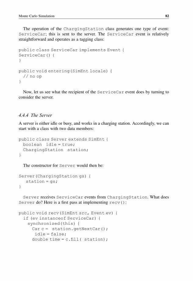
The operation of the ChargingStation class generates one type of event:
ServiceCar; this is sent to the server. The ServiceCar event is relatively
straightforward and operates as a tagging class:
public class ServiceCar implements Event {
ServiceCar() {
}
public void entering(SimEnt locale) {
// no op
}
Now, let us see what the recipient of the ServiceCar event does by turning to
consider the server.
4.4.4 The Server
A server is either idle or busy, and works in a charging station. Accordingly, we can
start with a class with two data members:
public class Server extends SimEnt {
boolean idle = true;
ChargingStation station;
}
The constructor for Server would then be:
Server(ChargingStation gs) {
station = gs;
}
Server receives ServiceCar events from ChargingStation. What does
Server do? Here is a first pass at implementing recv():
public void recv(SimEnt src, Event ev) {
if (ev instanceof ServiceCar) {
synchronized(this) {
Car c = station.getNextCar();
idle = false;
double time = c.fill( station);
Monte Carlo Simulation 82
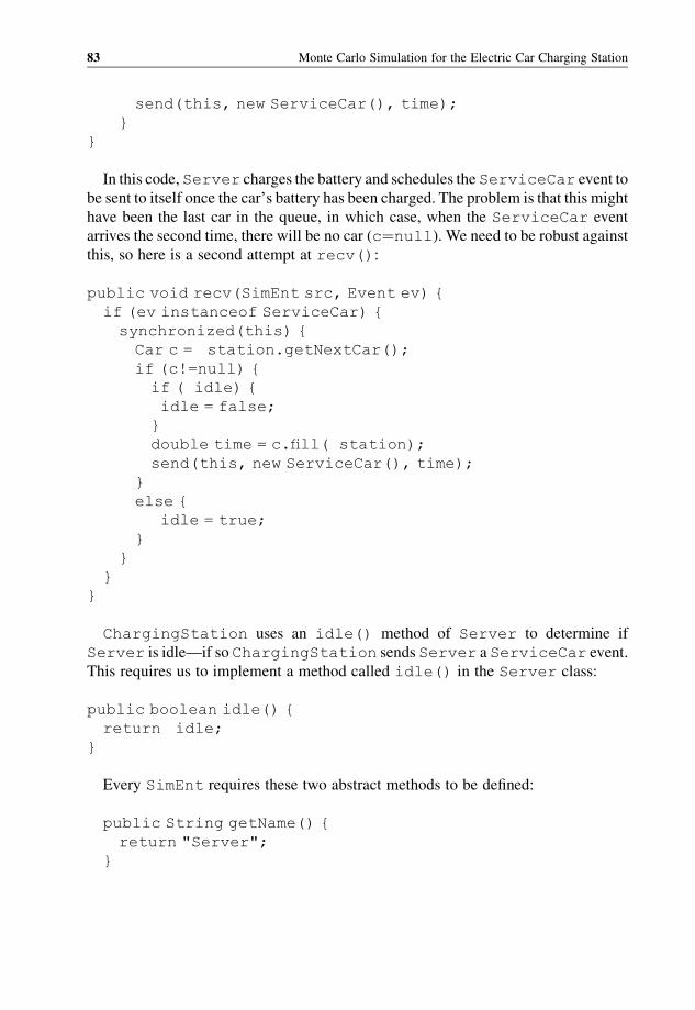
send(this, new ServiceCar(), time);
}
}
In this code, Server charges the battery and schedules the ServiceCar event to
be sent to itself once the car’s battery has been charged. The problem is that this might
have been the last car in the queue, in which case, when the ServiceCar event
arrives the second time, there will be no car (c¼null). We need to be robust against
this, so here is a second attempt at recv():
public void recv(SimEnt src, Event ev) {
if (ev instanceof ServiceCar) {
synchronized(this) {
Car c = station.getNextCar();
if (c!=null) {
if ( idle) {
idle = false;
}
double time = c.fill( station);
send(this, new ServiceCar(), time);
}
else {
idle = true;
}
}
}
}
ChargingStation uses an idle() method of Server to determine if
Server is idle—if so ChargingStation sends Server a ServiceCar event.
This requires us to implement a method called idle() in the Server class:
public boolean idle() {
return idle;
}
Every SimEnt requires these two abstract methods to be defined:
public String getName() {
return "Server";
}
83 Monte Carlo Simulation for the Electric Car Charging Station
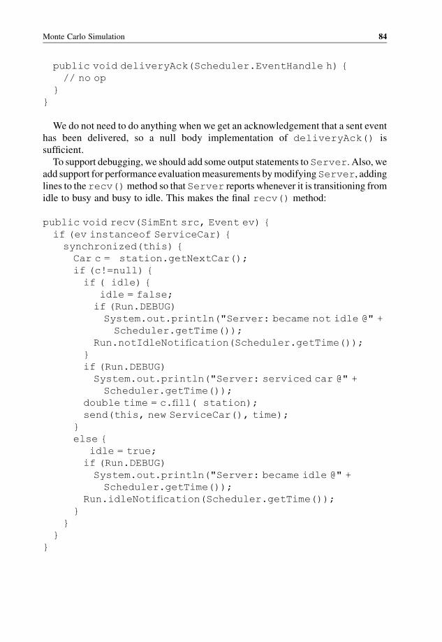
public void deliveryAck(Scheduler.EventHandle h) {
// no op
}
}
We do not need to do anything when we get an acknowledgement that a sent event
has been delivered, so a null body implementation of deliveryAck() is
sufficient.
To support debugging, we should add some output statements toServer. Also, we
add support for performance evaluationmeasurements bymodifyingServer, adding
lines to the recv()method so that Server reports whenever it is transitioning from
idle to busy and busy to idle. This makes the final recv() method:
public void recv(SimEnt src, Event ev) {
if (ev instanceof ServiceCar) {
synchronized(this) {
Car c = station.getNextCar();
if (c!=null) {
if ( idle) {
idle = false;
if (Run.DEBUG)
System.out.println("Server: became not idle @" +
Scheduler.getTime());
Run.notIdleNotification(Scheduler.getTime());
}
if (Run.DEBUG)
System.out.println("Server: serviced car @" +
Scheduler.getTime());
double time = c.fill( station);
send(this, new ServiceCar(), time);
}
else {
idle = true;
if (Run.DEBUG)
System.out.println("Server: became idle @" +
Scheduler.getTime());
Run.idleNotification(Scheduler.getTime());
}
}
}
}
Monte Carlo Simulation 84
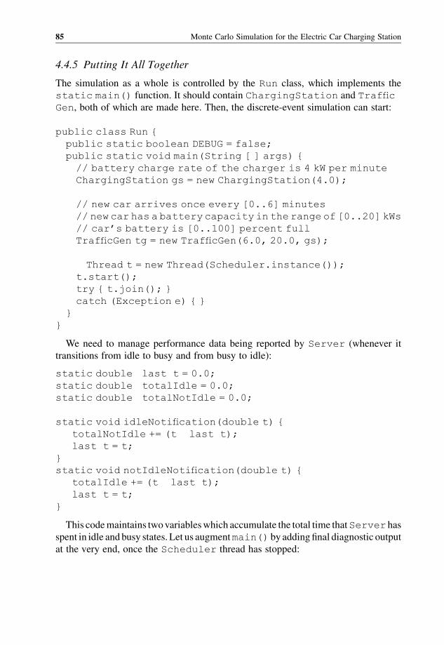
4.4.5 Putting It All Together
The simulation as a whole is controlled by the Run class, which implements the
static main() function. It should contain ChargingStation and Traffic
Gen, both of which are made here. Then, the discrete-event simulation can start:
public class Run {
public static boolean DEBUG = false;
public static void main(String [ ] args) {
// battery charge rate of the charger is 4 kW per minute
ChargingStation gs = new ChargingStation(4.0);
// new car arrives once every [0..6] minutes
// new car has a battery capacity in the range of [0..20] kWs
// car’s battery is [0..100] percent full
TrafficGen tg = new TrafficGen(6.0, 20.0, gs);
Thread t = new Thread(Scheduler.instance());
t.start();
try { t.join(); }
catch (Exception e) { }
}
}
We need to manage performance data being reported by Server (whenever it
transitions from idle to busy and from busy to idle):
static double last t = 0.0;
static double totalIdle = 0.0;
static double totalNotIdle = 0.0;
static void idleNotification(double t) {
totalNotIdle += (t last t);
last t = t;
}
static void notIdleNotification(double t) {
totalIdle += (t last t);
last t = t;
}
This codemaintains twovariableswhich accumulate the total time thatServer has
spent in idle and busy states. Let us augmentmain() by addingfinal diagnostic output
at the very end, once the Scheduler thread has stopped:
85 Monte Carlo Simulation for the Electric Car Charging Station
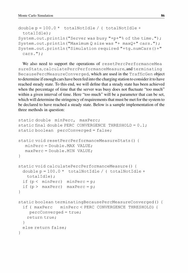
double p = 100.0 * totalNotIdle / ( totalNotIdle +
totalIdle);
System.out.println("Server was busy "+p+"% of the time.");
System.out.println("Maximum Q size was "+ maxQ+" cars.");
System.out.println("Simulation required "+tg.numCars()+"
cars.");
We also need to support the operations of resetPercPerformanceMea
sureStats,calculatePercPerformanceMeasure, andterminating
BecausePercMeasureConverged, which are used in the TrafficGen object
to determine if enough cars havebeen fed into the charging station to consider it to have
reached steady state. To this end, we will define that a steady state has been achieved
when the percentage of time that the server was busy does not fluctuate “too much”
within a given interval of time. Here “too much” will be a parameter that can be set,
which will determine the stringency of requirements that must bemet for the system to
be declared to have reached a steady state. Below is a sample implementation of the
three methods in question:
static double minPerc, maxPerc;
static final double PERC CONVERGENCE THRESHOLD = 0.1;
static boolean percConverged = false;
static void resetPercPerformanceMeasureStats() {
minPerc = Double.MAX VALUE;
maxPerc = Double.MIN VALUE;
}
static void calculatePercPerformanceMeasure() {
double p = 100.0 * totalNotIdle / ( totalNotIdle +
totalIdle);
if (p < minPerc) minPerc = p;
if (p > maxPerc) maxPerc = p;
}
static boolean terminatingBecausePercMeasureConverged() {
if ( maxPerc minPerc < PERC CONVERGENCE THRESHOLD) {
percConverged = true;
return true;
}
else return false;
}
Monte Carlo Simulation 86
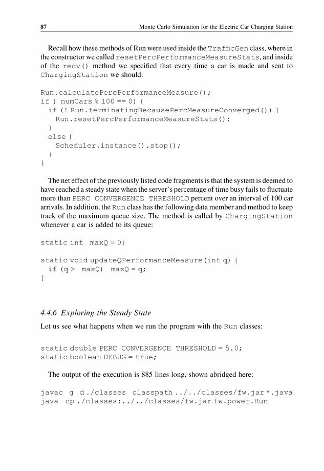
Recall how thesemethods of Runwere used inside the TrafficGen class, where in
the constructor we called resetPercPerformanceMeasureStats, and inside
of the recv() method we specified that every time a car is made and sent to
ChargingStation we should:
Run.calculatePercPerformanceMeasure();
if ( numCars % 100 == 0) {
if (! Run.terminatingBecausePercMeasureConverged()) {
Run.resetPercPerformanceMeasureStats();
}
else {
Scheduler.instance().stop();
}
}
The net effect of the previously listed code fragments is that the system is deemed to
have reached a steady statewhen the server’s percentage of time busy fails to fluctuate
more than PERC CONVERGENCE THRESHOLD percent over an interval of 100 car
arrivals. In addition, the Run class has the following data member and method to keep
track of the maximum queue size. The method is called by ChargingStation
whenever a car is added to its queue:
static int maxQ = 0;
static void updateQPerformanceMeasure(int q) {
if (q > maxQ) maxQ = q;
}
4.4.6 Exploring the Steady State
Let us see what happens when we run the program with the Run classes:
static double PERC CONVERGENCE THRESHOLD = 5.0;
static boolean DEBUG = true;
The output of the execution is 885 lines long, shown abridged here:
javac g d ./classes classpath ../../classes/fw.jar *.java
java cp ./classes:../../classes/fw.jar fw.power.Run
87 Monte Carlo Simulation for the Electric Car Charging Station
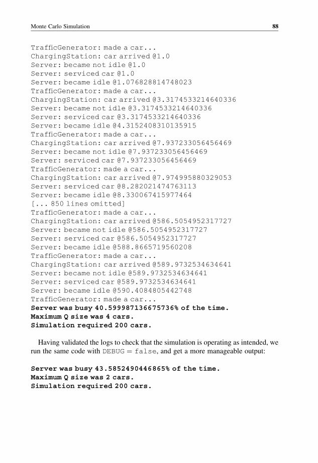
TrafficGenerator: made a car...
ChargingStation: car arrived @1.0
Server: became not idle @1.0
Server: serviced car @1.0
Server: became idle @1.076828814748023
TrafficGenerator: made a car...
ChargingStation: car arrived @3.3174533214640336
Server: became not idle @3.3174533214640336
Server: serviced car @3.3174533214640336
Server: became idle @4.3152408310135915
TrafficGenerator: made a car...
ChargingStation: car arrived @7.937233056456469
Server: became not idle @7.937233056456469
Server: serviced car @7.937233056456469
TrafficGenerator: made a car...
ChargingStation: car arrived @7.974995880329053
Server: serviced car @8.282021474763113
Server: became idle @8.330067415977464
[... 850 lines omitted]
TrafficGenerator: made a car...
ChargingStation: car arrived @586.5054952317727
Server: became not idle @586.5054952317727
Server: serviced car @586.5054952317727
Server: became idle @588.8665719560208
TrafficGenerator: made a car...
ChargingStation: car arrived @589.9732534634641
Server: became not idle @589.9732534634641
Server: serviced car @589.9732534634641
Server: became idle @590.4084805442748
TrafficGenerator: made a car...
Server was busy 40.599987136675736% of the time.Maximum Q size was 4 cars.Simulation required 200 cars.
Having validated the logs to check that the simulation is operating as intended, we
run the same code with DEBUG ¼ false, and get a more manageable output:
Server was busy 43.5852490446865% of the time.Maximum Q size was 2 cars.Simulation required 200 cars.
Monte Carlo Simulation 88
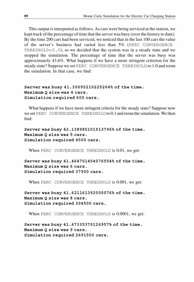
This output is interpreted as follows. As cars were being serviced at the station, we
kept track of the percentage of time that the server was busy (over the history to date).
By the time 200 cars had been serviced, we noticed that in the last 100 cars the value
of the server’s business had varied less than 5% (PERC CONVERGENCE
THRESHOLD¼5.0), so we decided that the system was in a steady state and we
stopped the simulation. The percentage of time that the server was busy was
approximately 43.6%. What happens if we have a more stringent criterion for the
steady state? Supposewe setPERC CONVERGENCE THRESHOLD to 1.0 and rerun
the simulation. In that case, we find:
Server was busy 41.30095210225264% of the time.Maximum Q size was 4 cars.Simulation required 600 cars.
What happens if we have more stringent criteria for the steady state? Suppose now
we setPERC CONVERGENCE THRESHOLD to 0.1 and rerun the simulation.We then
find:
Server was busy 42.138985101913796% of the time.Maximum Q size was 5 cars.Simulation required 4500 cars.
When PERC CONVERGENCE THRESHOLD is 0.01, we get:
Server was busy 41.464701454076554% of the time.Maximum Q size was 6 cars.Simulation required 37900 cars.
When PERC CONVERGENCE THRESHOLD is 0.001, we get:
Server was busy 41.621161392000076% of the time.Maximum Q size was 8 cars.Simulation required 304500 cars.
When PERC CONVERGENCE THRESHOLD is 0.0001, we get:
Server was busy 41.67335379126957% of the time.Maximum Q size was 9 cars.Simulation required 2691500 cars.
89 Monte Carlo Simulation for the Electric Car Charging Station
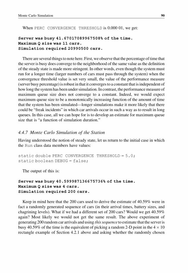
When PERC CONVERGENCE THRESHOLD is 0.000 01, we get:
Server was busy 41.67017089967508% of the time.Maximum Q size was 11 cars.Simulation required 20990500 cars.
There are several things to note here. First, weobserve that the percentage of time that
the server is busy does converge to the neighborhood of the same value as the definition
of the steady state is mademore stringent. In other words, even though the systemmust
run for a longer time (larger numbers of cars must pass through the system) when the
convergence threshold value is set very small, the value of the performance measure
(server busy percentage) is robust in that it converges to a constant that is independent of
how long the systemhas beenunder simulation. In contrast, the performancemeasure of
maximum queue size does not converge to a constant. Indeed, we would expect
maximum queue size to be a monotonically increasing function of the amount of time
that the system has been simulated—longer simulations make it more likely that there
could be “freak incidents” in which car arrivals occur in such a way as to result in long
queues. In this case, all we can hope for is to develop an estimate for maximum queue
size that is “a function of simulation duration.”
4.4.7 Monte Carlo Simulation of the Station
Having understood the notion of steady state, let us return to the initial case in which
the Run class data members have values:
static double PERC CONVERGENCE THRESHOLD = 5.0;
static boolean DEBUG = false;
The output of this is:
Server was busy 40.599987136675736% of the time.Maximum Q size was 4 cars.Simulation required 200 cars.
Keep in mind here that the 200 cars used to derive the estimate of 40.59% were in
fact a randomly generated sequence of cars (in their arrival times, battery sizes, and
chagrining levels). What if we had a different set of 200 cars? Would we get 40.59%
again? Most likely we would not get the same result. The above experiment of
generating 200 randomcar arrivals and using this sequence to estimate that the server is
busy 40.59% of the time is the equivalent of picking a random 2-D point in the 4� 10
rectangle example of Section 4.2.1 above and asking whether the randomly chosen
Monte Carlo Simulation 90
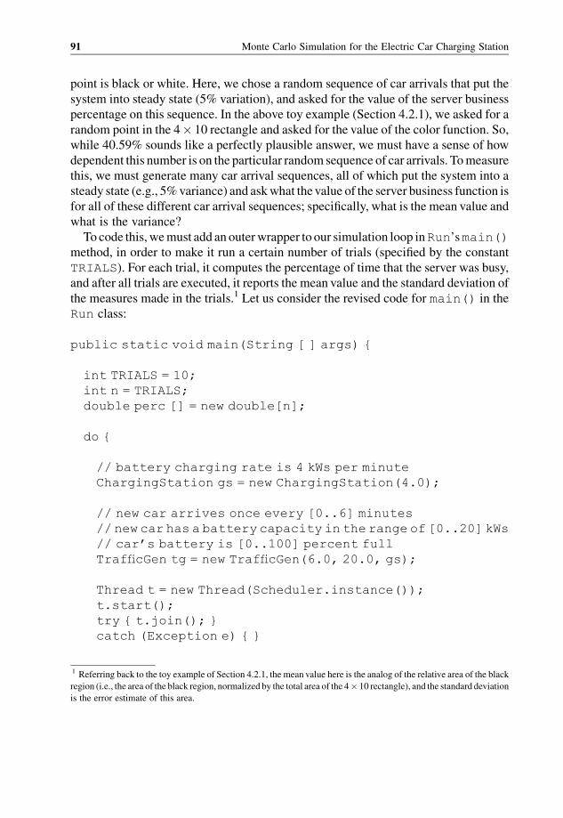
point is black or white. Here, we chose a random sequence of car arrivals that put the
system into steady state (5% variation), and asked for the value of the server business
percentage on this sequence. In the above toy example (Section 4.2.1), we asked for a
random point in the 4� 10 rectangle and asked for the value of the color function. So,
while 40.59% sounds like a perfectly plausible answer, we must have a sense of how
dependent this number is on the particular random sequence of car arrivals. Tomeasure
this, we must generate many car arrival sequences, all of which put the system into a
steady state (e.g., 5%variance) and askwhat thevalue of the server business function is
for all of these different car arrival sequences; specifically, what is the mean value and
what is the variance?
To code this, wemust add an outerwrapper to our simulation loop inRun’smain()
method, in order to make it run a certain number of trials (specified by the constant
TRIALS). For each trial, it computes the percentage of time that the server was busy,
and after all trials are executed, it reports the mean value and the standard deviation of
the measures made in the trials.1 Let us consider the revised code for main() in the
Run class:
public static void main(String [ ] args) {
int TRIALS = 10;
int n = TRIALS;
double perc [] = new double[n];
do {
// battery charging rate is 4 kWs per minute
ChargingStation gs = new ChargingStation(4.0);
// new car arrives once every [0..6] minutes
// new car has a battery capacity in the range of [0..20] kWs
// car’s battery is [0..100] percent full
TrafficGen tg = new TrafficGen(6.0, 20.0, gs);
Thread t = new Thread(Scheduler.instance());
t.start();
try { t.join(); }
catch (Exception e) { }
1 Referring back to the toy example of Section 4.2.1, the mean value here is the analog of the relative area of the black
region (i.e., the area of the black region, normalized by the total area of the 4� 10 rectangle), and the standard deviation
is the error estimate of this area.
91 Monte Carlo Simulation for the Electric Car Charging Station

double p = 100.0 * totalNotIdle / ( totalNotIdle +
totalIdle);
System.out.println("Server was busy "+p+"% of the
time.");
System.out.println("Maximum Q size was "+ maxQ+"
cars.");
System.out.println("Simulation required "+tg.numCars()
+" cars.");
n ;
perc[n] += 100.0 * totalNotIdle / ( totalNotIdle +
totalIdle);
Scheduler.instance().reset();
last t = 0.0;
totalIdle = 0.0;
totalNotIdle = 0.0;
}
while (n > 0);
double meanperc = 0.0;
for (n=0;n<TRIALS;n++) meanperc += perc[n];
meanperc /= (double)TRIALS;
double var = 0.0;
for (n=0;n<TRIALS;n++) var += (perc[n] meanperc)*(perc
[n] meanperc);
var /= (double)TRIALS;
double dev = Math.sqrt(var);
System.out.println("Server was busy "+meanperc+"% of the
time, "+ "std="+dev);
}
When we run this code, we get the following output:
javac g d ./classes classpath ../../classes/fw.jar *.java
Note: ChargingStation.java uses unchecked or unsafe
operations.
Note: Recompile with Xlint:unchecked for details.
java cp ./classes:../../classes/fw.jar fw.power.Run
Monte Carlo Simulation 92

Server was busy 39.4602804160784% of the time.
Maximum Q size was 3 cars.
Simulation required 200 cars.
Server was busy 41.77209593885758% of the time.
Maximum Q size was 3 cars.
Simulation required 200 cars.
Server was busy 42.53583280696096% of the time.
Maximum Q size was 3 cars.
Simulation required 200 cars.
Server was busy 38.23658252611347% of the time.
Maximum Q size was 3 cars.
Simulation required 300 cars.
Server was busy 40.456579350640794% of the time.
Maximum Q size was 4 cars.
Simulation required 200 cars.
Server was busy 43.29099329492339% of the time.
Maximum Q size was 4 cars.
Simulation required 200 cars.
Server was busy 45.04948133086543% of the time.
Maximum Q size was 4 cars.
Simulation required 200 cars.
Server was busy 35.282865804116376% of the time.
Maximum Q size was 4 cars.
Simulation required 200 cars.
Server was busy 42.571069199527386% of the time.
Maximum Q size was 5 cars.
Simulation required 300 cars.
Server was busy 47.66183655340056% of the time.
Maximum Q size was 5 cars.
Simulation required 200 cars.
Server was busy 41.63176172214844% of the time,std=3.323358268112881
Note that the percentages vary in each trial. In addition, some trials require longer to
reach steady state (300 cars in the ninth trial versus 200 cars in the tenth trial). The trials
are each defined as a simulation which goes on long enough to bring the system to
steady state (less than 5% variance in the server business measure over the last 100 car
arrivals). Depending on the random sampling, sometimes this requires longer simula-
tions (more cars). The last line of the output shows the mean value (across 10 trials) of
the server business, and the standard deviation of the values measured in each of these
10 trials. Note that since each trial made different random choices, it produced
93 Monte Carlo Simulation for the Electric Car Charging Station

different performance measures (e.g., the ninth trial reported server busy 42% of the
time, while the tenth trial reported the server busy 47%of the time). Clearly, the values
have a non-zero spread, and so the standard deviation will be greater than zero. In fact,
we see in the last line that the standard deviation of the performance measures across
the 10 trials is 3.32.
Several questions could be posed at this point. The first is “what effectwill the number
of trials have on the value of the mean and the standard deviation?” Let us see what
occurs in practice. If we change TRIALS from 10 to 100, the last line of output reads:
Server was busy 41.422609654685814% of the time,std=3.0972676894689433
If we change TRIALS from 100 to 1000, the last line of output reads:
Server was busy 41.68637971516185% of the time,std=3.012845922105874
If we change TRIALS from 1000 to 10 000, the last line of output reads:
Server was busy 41.61390895944546% of the time,std=2.930492611147204
Note that themeanvalue of the performancemeasure does not changemuch, and the
standard deviation decreases only slightly. In particular, it seems unlikely that the
standard deviation would go down to zero as the number of trials increases. In other
words, the spread of performance measures when we run 10 trials is commensurate
with the spread of the measures when we run 10 000 trials (modeling these as normal
distributions), and not all of it is attributable to the number of trials. The reason for this
is thatmuch of the spread in thesevalues comes from the underlying 5%variability that
is permitted in the definition of steady state. To illustrate this, let us set TRIALS to
1000 and vary the PERC CONVERGENCE THRESHOLD.
WithTRIALS set to 1000 andPERC CONVERGENCE THRESHOLD to 5%,weget:
Server was busy 41.68637971516185% of the time,std=3.012845922105874
With TRIALS set to 1000 and PERC CONVERGENCE THRESHOLD to 1%, we
get:
Server was busy 41.57993260857031% of the time,std=1.7630972379477647
Monte Carlo Simulation 94
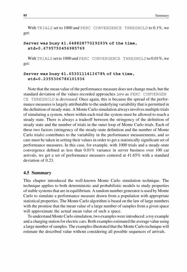
With TRIALS set to 1000 and PERC CONVERGENCE THRESHOLD to 0.1%, we
get:
Server was busy 41.64882877029293% of the time,std=0.6795750456985769
WithTRIALS set to 1000 andPERC CONVERGENCE THRESHOLD to 0.01%,we
get:
Server was busy 41.6530111413678% of the time,std=0.2355306786101936
Note that themeanvalue of the performancemeasure does not changemuch, but the
standard deviation of the values recorded approaches zero as PERC CONVERGEN
CE THRESHOLD is decreased. Once again, this is because the spread of the perfor-
mancemeasures is largely attributable to the underlying variability that is permitted in
the definition of steady state. AMonte Carlo simulation always involvesmultiple trials
of simulating a system, where within each trial the system must be allowed to reach a
steady state. There is always a tradeoff between the stringency of the definition of
steady state and the number of trials in the outer loop of Monte Carlo trials. Each of
these two factors (stringency of the steady-state definition and the number of Monte
Carlo trials) contributes to the variability in the performance measurements, and so
care must be taken in setting their values in order to get a statistically significant set of
performance measures. In this case, for example, with 1000 trials and a steady-state
convergence defined as less than 0.01% variance in server business over 100 car
arrivals, we get a set of performance measures centered at 41.65% with a standard
deviation of 0.23.
4.5 Summary
This chapter introduced the well-known Monte Carlo simulation technique. The
technique applies to both deterministic and probabilistic models to study properties
of stable systems that are in equilibrium.A randomnumber generator is used byMonte
Carlo to simulate a performance measure drawn from a population with appropriate
statistical properties. The Monte Carlo algorithm is based on the law of large numbers
with the promise that the mean value of a large number of samples from a given space
will approximate the actual mean value of such a space.
To understandMonteCarlo simulation, two exampleswere introduced: a toy example
and a charging station for electric cars. Both examples estimated the averagevalue using
a large number of samples. The examples illustrated that theMonte Carlo techniquewill
estimate the described value without considering all possible sequences of arrivals.
95 Summary
Recommended Reading
[1] R. Y. Rubinstein andD. P. Kroese, Simulation and theMonte CarloMethod, 2nd Edition, JohnWiley
& Sons, Inc., 2008.
[2] C. P. Robert and G. Casella, Monte Carlo Statistical Methods, 2nd Edition, Springer Texts in
Statistics, 2004.
[3] P. Glasserman, Monte Carlo Methods in Financial Engineering, Springer Stochastic Modeling and
Applied Probability Series, 2003.
[4] C. Z. Mooney, Monte Carlo Simulation, Sage, 1997.
Monte Carlo Simulation 96
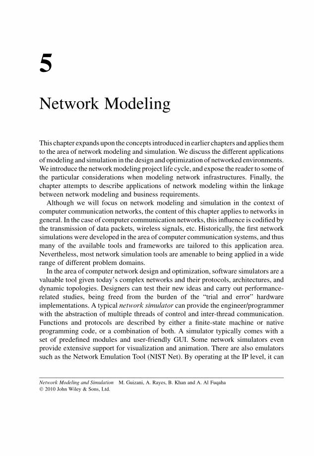
5
Network Modeling
This chapter expands upon the concepts introduced in earlier chapters and applies them
to the area of network modeling and simulation. We discuss the different applications
ofmodeling and simulation in the design andoptimization of networked environments.
We introduce the networkmodeling project life cycle, and expose the reader to some of
the particular considerations when modeling network infrastructures. Finally, the
chapter attempts to describe applications of network modeling within the linkage
between network modeling and business requirements.
Although we will focus on network modeling and simulation in the context of
computer communication networks, the content of this chapter applies to networks in
general. In the case of computer communication networks, this influence is codified by
the transmission of data packets, wireless signals, etc. Historically, the first network
simulations were developed in the area of computer communication systems, and thus
many of the available tools and frameworks are tailored to this application area.
Nevertheless, most network simulation tools are amenable to being applied in a wide
range of different problem domains.
In the area of computer network design and optimization, software simulators are a
valuable tool given today’s complex networks and their protocols, architectures, and
dynamic topologies. Designers can test their new ideas and carry out performance-
related studies, being freed from the burden of the “trial and error” hardware
implementations. A typical network simulator can provide the engineer/programmer
with the abstraction of multiple threads of control and inter-thread communication.
Functions and protocols are described by either a finite-state machine or native
programming code, or a combination of both. A simulator typically comes with a
set of predefined modules and user-friendly GUI. Some network simulators even
provide extensive support for visualization and animation. There are also emulators
such as the Network Emulation Tool (NIST Net). By operating at the IP level, it can
Network Modeling and Simulation M. Guizani, A. Rayes, B. Khan and A. Al Fuqaha
� 2010 John Wiley & Sons, Ltd.
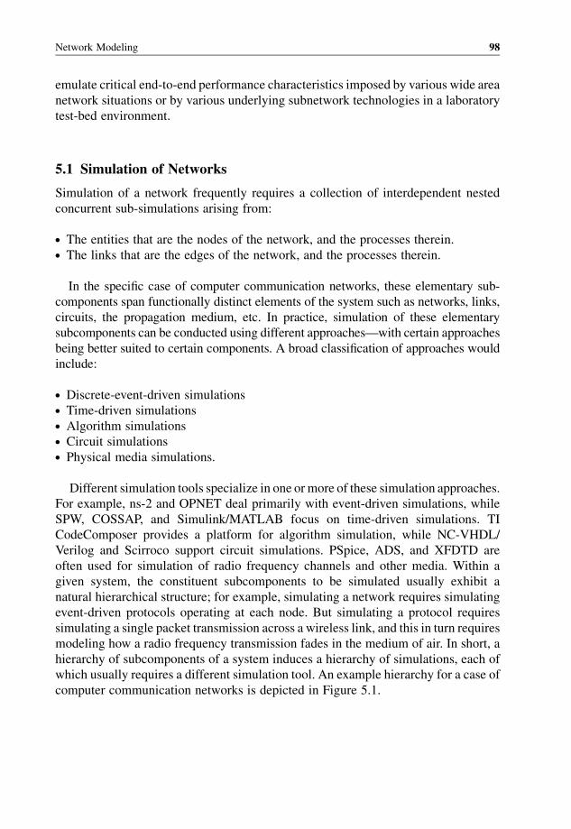
emulate critical end-to-end performance characteristics imposed by various wide area
network situations or by various underlying subnetwork technologies in a laboratory
test-bed environment.
5.1 Simulation of Networks
Simulation of a network frequently requires a collection of interdependent nested
concurrent sub-simulations arising from:
. The entities that are the nodes of the network, and the processes therein.
. The links that are the edges of the network, and the processes therein.
In the specific case of computer communication networks, these elementary sub-
components span functionally distinct elements of the system such as networks, links,
circuits, the propagation medium, etc. In practice, simulation of these elementary
subcomponents can be conducted using different approaches—with certain approaches
being better suited to certain components. A broad classification of approaches would
include:
. Discrete-event-driven simulations
. Time-driven simulations
. Algorithm simulations
. Circuit simulations
. Physical media simulations.
Different simulation tools specialize in one ormore of these simulation approaches.
For example, ns-2 and OPNET deal primarily with event-driven simulations, while
SPW, COSSAP, and Simulink/MATLAB focus on time-driven simulations. TI
CodeComposer provides a platform for algorithm simulation, while NC-VHDL/
Verilog and Scirroco support circuit simulations. PSpice, ADS, and XFDTD are
often used for simulation of radio frequency channels and other media. Within a
given system, the constituent subcomponents to be simulated usually exhibit a
natural hierarchical structure; for example, simulating a network requires simulating
event-driven protocols operating at each node. But simulating a protocol requires
simulating a single packet transmission across a wireless link, and this in turn requires
modeling how a radio frequency transmission fades in the medium of air. In short, a
hierarchy of subcomponents of a system induces a hierarchy of simulations, each of
which usually requires a different simulation tool. An example hierarchy for a case of
computer communication networks is depicted in Figure 5.1.
Network Modeling 98
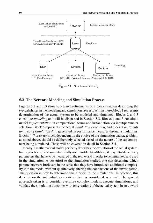
5.2 The Network Modeling and Simulation Process
Figures 5.2 and 5.3 show successive refinements of a block diagram describing the
typical phases in themodeling and simulation process.Within these, block 1 represents
determination of the actual system to be modeled and simulated. Blocks 2 and 3
constitute modeling and will be discussed in Section 5.3. Blocks 4 and 5 constitute
model implementation in computational terms and instantiation via input/parameter
selection. Block 6 represents the actual simulation execution, and block 7 represents
analysis of simulation data generated on performance measures through simulations.
Blocks 4–7 are very much dependent on the choice of the simulation package, which,
as noted above, should be deliberately selected based on the nature of the subcompo-
nent being simulated. These will be covered in detail in Section 5.4.
Ideally, amathematicalmodel perfectly describes the evolution of the actual system,
but in practice this is computationally not feasible. In addition, it may introduce many
parameters that have to bemeasured in the real world in order to be initialized and used
in the simulation. A posteriori to the simulation studies, one can determine which
parameters were irrelevant in the sense that they have introduced additional complex-
ity into the model without qualitatively altering the conclusions of the investigation.
The question is how to determine this a priori to the simulations. In practice, this
depends on the individual’s experience and is considered as an art. The general
approach taken is to consider evermore complex models, execute simulations, and
validate the simulation outcomes with observations of the actual system in an upward
Networks
Links
DSP Circuits Medium
Event-Driven Simulations:
ns-2, OPNET
Time-Driven Simulations: SPW,
COSSAP, Simulink/MATLAB
Packets, Messages, Flows
Technology
Algorithm simulations:
TI CodeComposer
Circuit simulations:
NC-{VHDL/Verilog}, Scirroco
Medium simulations
PSpice, ADS, XFDTD
Waveforms
Figure 5.1 Simulation hierarchy
99 The Network Modeling and Simulation Process
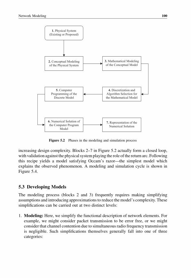
increasing design complexity. Blocks 2–7 in Figure 5.2 actually form a closed loop,
with validation against the physical systemplaying the role of the return arc. Following
this recipe yields a model satisfying Occam’s razor—the simplest model which
explains the observed phenomenon. A modeling and simulation cycle is shown in
Figure 5.4.
5.3 Developing Models
The modeling process (blocks 2 and 3) frequently requires making simplifying
assumptions and introducing approximations to reduce themodel’s complexity. These
simplifications can be carried out at two distinct levels:
1. Modeling: Here, we simplify the functional description of network elements. For
example, we might consider packet transmission to be error free, or we might
consider that channel contention due to simultaneous radio frequency transmission
is negligible. Such simplifications themselves generally fall into one of three
categories:
1. Physical System
(Existing or Proposed)
2. Conceptual Modeling
of the Physical System
5. Computer
Programming of the
Discrete Model
6. Numerical Solution of
the Computer Program
Model
3. Mathematical Modeling
of the Conceptual Model
4. Discretization and
Algorithm Selection for
the Mathematical Model
7. Representation of the
Numerical Solution
Figure 5.2 Phases in the modeling and simulation process
Network Modeling 100
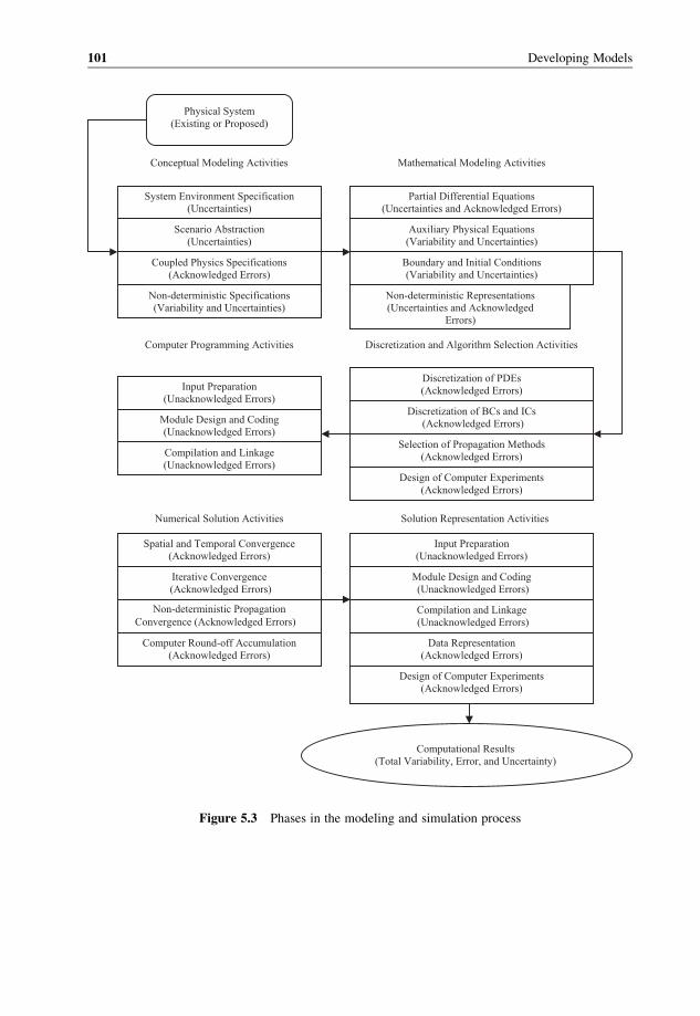
Physical System
(Existing or Proposed)
System Environment Specification
(Uncertainties)
Scenario Abstraction
(Uncertainties)
Coupled Physics Specifications
(Acknowledged Errors)
Non-deterministic Specifications
(Variability and Uncertainties)
Partial Differential Equations
(Uncertainties and Acknowledged Errors)
Auxiliary Physical Equations
(Variability and Uncertainties)
Boundary and Initial Conditions
(Variability and Uncertainties)
Non-deterministic Representations
(Uncertainties and Acknowledged
Errors)
Conceptual Modeling Activities Mathematical Modeling Activities
Input Preparation
(Unacknowledged Errors)
Module Design and Coding
(Unacknowledged Errors)
Compilation and Linkage
(Unacknowledged Errors)
Discretization of PDEs
(Acknowledged Errors)
Discretization of BCs and ICs
(Acknowledged Errors)
Selection of Propagation Methods
(Acknowledged Errors)
Design of Computer Experiments
(Acknowledged Errors)
Spatial and Temporal Convergence
(Acknowledged Errors)
Iterative Convergence
(Acknowledged Errors)
Non-deterministic Propagation
Convergence (Acknowledged Errors)
Computer Round-off Accumulation
(Acknowledged Errors)
Input Preparation
(Unacknowledged Errors)
Module Design and Coding
(Unacknowledged Errors)
Compilation and Linkage
(Unacknowledged Errors)
Data Representation
(Acknowledged Errors)
Design of Computer Experiments
(Acknowledged Errors)
Computer Programming Activities Discretization and Algorithm Selection Activities
Numerical Solution Activities Solution Representation Activities
Computational Results
(Total Variability, Error, and Uncertainty)
Figure 5.3 Phases in the modeling and simulation process
101 Developing Models
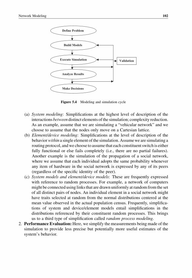
(a) System modeling: Simplifications at the highest level of description of the
interactions between distinct elements of the simulation; complexity reduction.
As an example, assume that we are simulating a “vehicular network” and we
choose to assume that the nodes only move on a Cartesian lattice.
(b) Element/device modeling: Simplifications at the level of description of the
behaviorwithin a single element of the simulation.Assumewe are simulating a
routing protocol, andwe choose to assume that each constituent switch is either
fully functional or else fails completely (i.e., there are no partial failures).
Another example is the simulation of the propagation of a social network,
where we assume that each individual adopts the same probability whenever
any item of hardware in the social network is expressed by any of its peers
(regardless of the specific identity of the peer).
(c) System models and element/device models: These are frequently expressed
with reference to random processes. For example, a network of computers
might be connected using links that are drawn uniformly at random from the set
of all distinct pairs of nodes. An individual element in a social network might
have traits selected at random from the normal distributions centered at the
mean value observed in the actual population census. Frequently, simplifica-
tions of system and device/element models entail simplifications in the
distributions referenced by their constituent random processes. This brings
us to a third type of simplification called random process modeling.
2. Performance Evaluation:Here, we simplify the measurements being made of the
simulation to provide less precise but potentially more useful estimates of the
system’s behavior.
Define Problem
Build Models
Execute Simulation
Analyze Results
Make Decisions
Validation
Figure 5.4 Modeling and simulation cycle
Network Modeling 102
5.4 Network Simulation Packages
Asnoted earlier, blocks 4–7 areverymuch dependent on the choice of simulation tools.
Some examples of academic simulators include the following:
. REAL is a simulator for studying the dynamic behavior of flow and congestion
control schemes in packet switched data networks. Network topology, protocols,
data, and control parameters are represented byScenarios,which are described using
NetLanguage, a simple ASCII representation of the network. About 30 modules are
provided which can exactly emulate the actions of several well-known flow control
protocols.. INSANE is a network simulator designed to test various IP-over-ATM algorithms
with realistic traffic loads derived from empirical traffic measurements. Its ATM
protocol stack provides real-time guarantees to ATM virtual circuits by using Rate
Controlled Static Priority (RCSP) queuing. A protocol similar to the Real-Time
Channel Administration Protocol (RCAP) is implemented for ATM signaling. A
graphical simulation monitor can provide an easy way to check the progress of
multiple running simulation processes.. NetSim is intended to offer a very detailed simulation of Ethernet, including realistic
modeling of signal propagation, the effect of the relative positions of stations on
events in the network, the collision detection and handling process, and the
transmission deferralmechanism.However, it cannot be extended to addressmodern
networks.. Maisie is a C-based language for hierarchical simulation, or, more specifically, a
language for parallel discrete-event simulation. A logical process is used to model
one or more physical processes; the events in the physical system are modeled by
message exchanges among the corresponding logical processes in the model. Users
can also migrate into recent extensions: Parsec and MOOSE (an object-oriented
extension).. OPNET (Optimized Network Engineering Tool) is an object-oriented simula-
tion environment that meets all these requirements and is the most powerful
general-purpose network simulator available today. OPNET’s comprehensive
analysis tool is especially ideal for interpreting and synthesizing output data. A
discrete-event simulation of the call and routing signaling was developed using a
number of OPNET’s unique features such as the dynamic allocation of pro-
cesses to model virtual circuits transiting through an ATM switch. Moreover, its
built-in Proto-C language support gives it the ability to realize almost any
function and protocol. OPNET provides a comprehensive development envi-
ronment for the specification, simulation, and performance analysis of commu-
nication networks. A large range of communication systems from a single LAN
to global satellite networks can be supported. Discrete-event simulations are
103 Network Simulation Packages
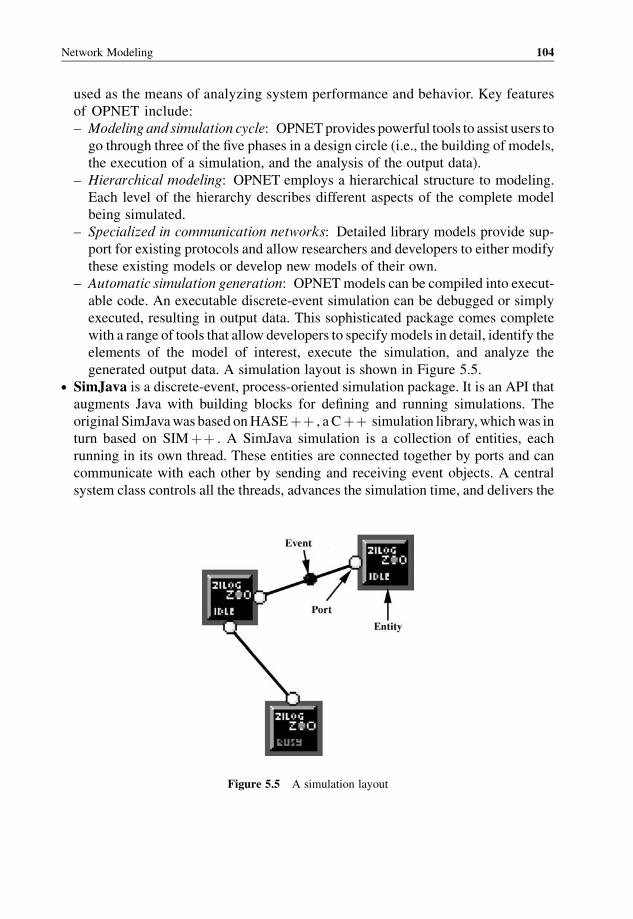
used as the means of analyzing system performance and behavior. Key features
of OPNET include:
– Modeling and simulation cycle: OPNETprovides powerful tools to assist users to
go through three of the five phases in a design circle (i.e., the building of models,
the execution of a simulation, and the analysis of the output data).
– Hierarchical modeling: OPNET employs a hierarchical structure to modeling.
Each level of the hierarchy describes different aspects of the complete model
being simulated.
– Specialized in communication networks: Detailed library models provide sup-
port for existing protocols and allow researchers and developers to either modify
these existing models or develop new models of their own.
– Automatic simulation generation: OPNETmodels can be compiled into execut-
able code. An executable discrete-event simulation can be debugged or simply
executed, resulting in output data. This sophisticated package comes complete
with a range of tools that allow developers to specifymodels in detail, identify the
elements of the model of interest, execute the simulation, and analyze the
generated output data. A simulation layout is shown in Figure 5.5.. SimJava is a discrete-event, process-oriented simulation package. It is an API that
augments Java with building blocks for defining and running simulations. The
original SimJavawas based onHASEþþ , a Cþþ simulation library,whichwas in
turn based on SIMþþ . A SimJava simulation is a collection of entities, each
running in its own thread. These entities are connected together by ports and can
communicate with each other by sending and receiving event objects. A central
system class controls all the threads, advances the simulation time, and delivers the
Figure 5.5 A simulation layout
Network Modeling 104
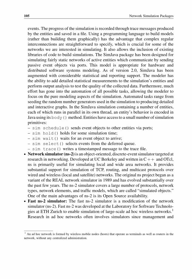
events. The progress of the simulation is recorded through trace messages produced
by the entities and saved in a file. Using a programming language to build models
(rather than building them graphically) has the advantage that complex regular
interconnections are straightforward to specify, which is crucial for some of the
networks we are interested in simulating. It also allows the inclusion of existing
libraries of code to build simulations. The SimJava package has been designed for
simulating fairly static networks of active entities which communicate by sending
passive event objects via ports. This model is appropriate for hardware and
distributed software systems modeling. As of version 2.0, SimJava has been
augmented with considerable statistical and reporting support. The modeler has
the ability to add detailed statistical measurements to the simulation’s entities and
perform output analysis to test the quality of the collected data. Furthermore, much
effort has gone into the automation of all possible tasks, allowing the modeler to
focus on the pure modeling aspects of the simulation. Automated tasks range from
seeding the random number generators used in the simulation to producing detailed
and interactive graphs. In the SimJava simulation containing a number of entities,
each of which runs in parallel in its own thread, an entity’s behavior is encoded in
Java using itsbody()method. Entities have access to a small number of simulation
primitives:
– sim schedule() sends event objects to other entities via ports;
– sim hold() holds for some simulation time;
– sim wait() waits for an event object to arrive;
– sim select() selects events from the deferred queue.
– sim trace() writes a timestamped message to the trace file.. Network simulator (ns-2) is an object-oriented, discrete-event simulator targeted at
research in networking. Developed at UC Berkeley and written in Cþþ and OTcl,
ns is primarily useful for simulating local and wide area networks. It provides
substantial support for simulation of TCP, routing, and multicast protocols over
wired and wireless (local and satellite) networks. The original ns project began as a
variant of the REAL network simulator in 1989 and has evolved substantially over
the past few years. The ns-2 simulator covers a large number of protocols, network
types, network elements, and traffic models, which are called “simulated objects.”
One of the main advantages of ns-2 is its Open Source availability.. Fast ns-2 simulator: The fast ns-2 simulator is a modification of the network
simulator (ns-2). Fast ns-2 was developed at the Laboratory for Software Technolo-
gies at ETH Zurich to enable simulation of large-scale ad hoc wireless networks.1
Research in ad hoc networks often involves simulators since management and
1 An ad hoc network is formed by wireless mobile nodes (hosts) that operate as terminals as well as routers in the
network, without any centralized administration.
105 Network Simulation Packages
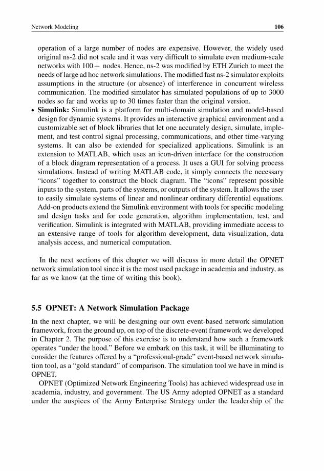
operation of a large number of nodes are expensive. However, the widely used
original ns-2 did not scale and it was very difficult to simulate even medium-scale
networks with 100þ nodes. Hence, ns-2 was modified by ETH Zurich to meet the
needs of large ad hoc network simulations. Themodified fast ns-2 simulator exploits
assumptions in the structure (or absence) of interference in concurrent wireless
communication. The modified simulator has simulated populations of up to 3000
nodes so far and works up to 30 times faster than the original version.. Simulink: Simulink is a platform for multi-domain simulation and model-based
design for dynamic systems. It provides an interactive graphical environment and a
customizable set of block libraries that let one accurately design, simulate, imple-
ment, and test control signal processing, communications, and other time-varying
systems. It can also be extended for specialized applications. Simulink is an
extension to MATLAB, which uses an icon-driven interface for the construction
of a block diagram representation of a process. It uses a GUI for solving process
simulations. Instead of writing MATLAB code, it simply connects the necessary
“icons” together to construct the block diagram. The “icons” represent possible
inputs to the system, parts of the systems, or outputs of the system. It allows the user
to easily simulate systems of linear and nonlinear ordinary differential equations.
Add-on products extend the Simulink environment with tools for specific modeling
and design tasks and for code generation, algorithm implementation, test, and
verification. Simulink is integrated with MATLAB, providing immediate access to
an extensive range of tools for algorithm development, data visualization, data
analysis access, and numerical computation.
In the next sections of this chapter we will discuss in more detail the OPNET
network simulation tool since it is the most used package in academia and industry, as
far as we know (at the time of writing this book).
5.5 OPNET: A Network Simulation Package
In the next chapter, we will be designing our own event-based network simulation
framework, from the ground up, on top of the discrete-event framework we developed
in Chapter 2. The purpose of this exercise is to understand how such a framework
operates “under the hood.” Before we embark on this task, it will be illuminating to
consider the features offered by a “professional-grade” event-based network simula-
tion tool, as a “gold standard” of comparison. The simulation tool we have in mind is
OPNET.
OPNET (Optimized Network Engineering Tools) has achieved widespread use in
academia, industry, and government. The US Army adopted OPNET as a standard
under the auspices of the Army Enterprise Strategy under the leadership of the
Network Modeling 106
US Army Office of the Director of Information Systems for Command, Control,
Communications and Computers. OPNET is widely used in universities as well as
many parts of the Department of Defense (DOD). OPNET supports visualization
through modeling objectives. It may be described as a communications-oriented
simulation language. The single most significant aspect of OPNET is that it provides
direct access to the source code coupled with an easy-to-use front end.
A generic approach to network modeling can be constructed using the OSI
Reference Model as its basis, as shown in Figure 5.6. This approach allows the
implementation of different network protocols which are compatible with the OSI
layer boundaries. Pedagogically, this approach has limitations. As illustrated in
Figure 5.6, any detailed implementation of an Ethernet model will not directly align
with the OSI Reference Model. Other protocols such as Fiber Distributed Data
Interface (FDDI) also do not perfectly align with the OSI Reference Model.
OPNET models are composed of three primary model layers: the process layer, the
node layer, and the network layer. The lowest modeling layer is the process layer. This
modeling hierarchy is illustrated in Figure 5.7. The process model in Figure 5.8 shows
Physical
Data Link
Network
Transport
Session
Presentation
Application
OSI Stack
Physical
MAC
Logical Link
IEEE 802.2LLC
PMD
PHY
MAC
Logical Link
FDDI Protocol Architecture
Figure 5.6 Reference models and architectures
Process Models
Node Models
Network Models
STD that defines a node
Individual Nodes and Stations
Networks and Subnetworks
Figure 5.7 OPNET model hierarchy
107 OPNET: A Network Simulation Package
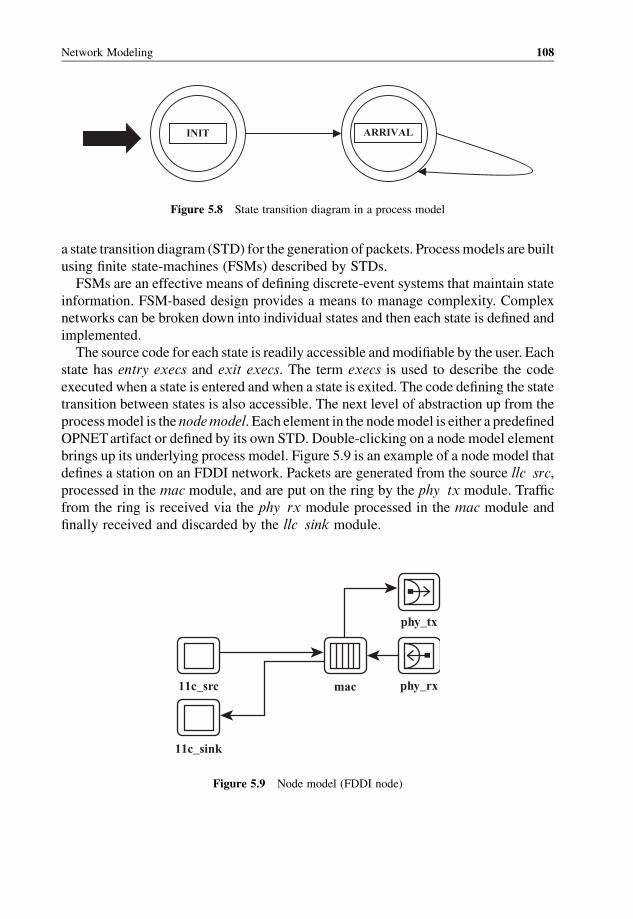
a state transition diagram (STD) for the generation of packets. Processmodels are built
using finite state-machines (FSMs) described by STDs.
FSMs are an effective means of defining discrete-event systems that maintain state
information. FSM-based design provides a means to manage complexity. Complex
networks can be broken down into individual states and then each state is defined and
implemented.
The source code for each state is readily accessible andmodifiable by the user. Each
state has entry execs and exit execs. The term execs is used to describe the code
executed when a state is entered and when a state is exited. The code defining the state
transition between states is also accessible. The next level of abstraction up from the
processmodel is the nodemodel. Each element in the nodemodel is either a predefined
OPNETartifact or defined by its own STD. Double-clicking on a node model element
brings up its underlying process model. Figure 5.9 is an example of a node model that
defines a station on an FDDI network. Packets are generated from the source llc src,
processed in the mac module, and are put on the ring by the phy tx module. Traffic
from the ring is received via the phy rx module processed in the mac module and
finally received and discarded by the llc sink module.
INIT ARRIVAL
Figure 5.8 State transition diagram in a process model
phy_tx
phy_rxmac11c_src
11c_sink
Figure 5.9 Node model (FDDI node)
Network Modeling 108
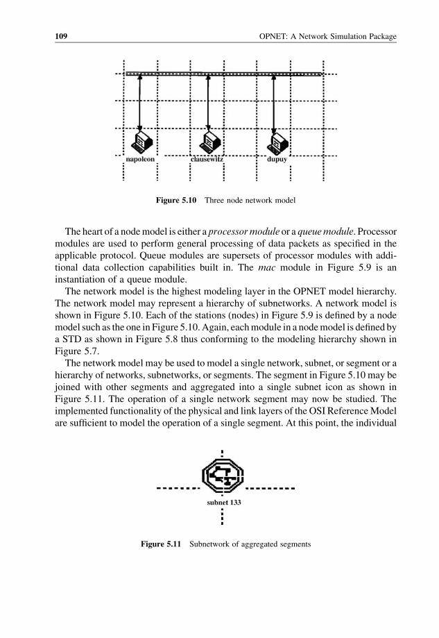
The heart of a nodemodel is either a processormodule or a queuemodule. Processor
modules are used to perform general processing of data packets as specified in the
applicable protocol. Queue modules are supersets of processor modules with addi-
tional data collection capabilities built in. The mac module in Figure 5.9 is an
instantiation of a queue module.
The network model is the highest modeling layer in the OPNET model hierarchy.
The network model may represent a hierarchy of subnetworks. A network model is
shown in Figure 5.10. Each of the stations (nodes) in Figure 5.9 is defined by a node
model such as the one in Figure 5.10.Again, eachmodule in a nodemodel is defined by
a STD as shown in Figure 5.8 thus conforming to the modeling hierarchy shown in
Figure 5.7.
The network model may be used to model a single network, subnet, or segment or a
hierarchy of networks, subnetworks, or segments. The segment in Figure 5.10 may be
joined with other segments and aggregated into a single subnet icon as shown in
Figure 5.11. The operation of a single network segment may now be studied. The
implemented functionality of the physical and link layers of the OSI ReferenceModel
are sufficient to model the operation of a single segment. At this point, the individual
Figure 5.10 Three node network model
Figure 5.11 Subnetwork of aggregated segments
109 OPNET: A Network Simulation Package
stations on the segmentmay be customized if amore detailed representation is desired.
Individual workstations or types of workstations may be specially modeled. Special
characteristics could be implemented by modifying the individual modules of the
station of interest or the physical network line connecting the stations. Many
modifications can be made via the built-in menus. However, modifications may be
made at the source code level should themenu choices not be fully satisfactory.Adding
network services in a TCP/IP network requires the implementation of the Internet
Protocol (IP). To simulate the operation of more than one segment, the functionality of
network layer servicesmust be added to themodel. The nodemodel of Figure 5.10may
be extended by adding modules to implement the IP and Address Resolution Protocol
(ARP). ARP tables are implemented statically with entries matching IP addresses to
MAC addresses.
5.6 Summary
In this chapter, different applications of modeling and simulation in the design and
optimization of networked environments have been discussed. The network modeling
project life cycle was introduced with network modeling and simulation processes.
Then, different network simulation tools/packages used in academia and industrywere
introduced, such as REAL, INSANE, NetSim, Maisie, OPNET, SimJava, Network
Simulator (ns-2), Fast ns-2 simulator, and Simulink.
Recommended Reading
[1] Online: http://www.opnet.com/
[2] Online: http://www.realsimulation.co.uk/
[3] Online: http://www.boson.com/AboutNetSim.html
[4] Online: http://www.kitchenlab.org/www/bmah/Software/Insane/
[5] Online: http://www.icsa.inf.ed.ac.uk/research/groups/hase/simjava/guide/tutorial.html
[6] Online: http://pcl.cs.ucla.edu/projects/maisie/tutorial/simulation/
Network Modeling 110
6
Designing and ImplementingCASiNO: A Network SimulationFramework
In Chapter 2, we designed a framework for discrete-event simulation (FDES) that we
used in a case study in Chapter 3. This showed how a FDES can be used to structure a
simulation study. Although the framework itself was quite small and consisted of only
three classes, Scheduler, SimEnt, and Event, the expressive power of the
framework made it easy to structure and reason about simulation design, and
implementation. The case study on communities of honeypots in Chapter 3 was an
example of a dynamic set of simulation entities that communicate with each other
using different types of concrete events in order to advance the state of the system over
time. In that study, the pattern of interconnectivity between the simulation entities was
dynamic and varied. This is often the case when considering simulations of dynamic
networks, since the topology of the network serves only as a relatively loose constraint
on the structure of the communication patterns.
Within a single network node, however, the situations that occur are more restricted
in scope, as we saw in Chapter 5. Simulations of a single entity/device (i.e. within a
single network node) lend themselves to more specialized frameworks that make
setting up and conducting intra-device simulation easier. Usually network software
(within a single node) is organized into layers, with very well defined communication
boundaries. Because the interfaces between these “layers” and “modules” are well
defined, the implementations can be updated without disturbing the operating system
as a whole. This enables abstraction and modular scalable design. In this section, we
will define a framework that will allow for modular specification and assembly of
Network Modeling and Simulation M. Guizani, A. Rayes, B. Khan and A. Al Fuqaha
� 2010 John Wiley & Sons, Ltd.
dataflow processing modules within a single device. We call this framework the
Component Architecture for Simulating Network Objects (CASiNO). The framework
described here is a compact Java framework based on an earlier heavy Cþþframework of the same name exposited by the authors in [1,2]. The framework
we will design and implement in this chapter is an extension of the Framework for
Discrete Event Simulation (FDES) described in Chapter 2. Our purpose is to make the
general-purpose FDES framework more specialized and better suited for building
distributed protocol simulations.
6.1 Overview
The CASiNO framework was originally based on conduits. We feel that it is worth
comparing CASiNO to a currently popular network simulator called ns [14]. If
CASiNO is used to build a network simulator, the resulting simulator and ns would
indeed have some commonalities in their architecture. The counterpart of the ns
scheduler is the FDES scheduler. Both Scheduler classes run by selecting and
executing the next earliest event scheduled. One of the differences between the ns and
the CASiNO codes is that ns, whilewritten in Java, has an “OTcl” interpreter as a front
end. Nevertheless, ns supports a class hierarchy in Cþþ and a similar class hierarchy
within theOTcl interpreter, thus allowing split-level programming.Another difference
is that the CASiNO framework is designed for actually implementing a network
protocol as an object-oriented software simulation. CASiNO itself is not a simulator
but an object-oriented framework for developing network protocols and simulations.
An object-oriented application is a set of objects working together to achieve a
commongoal. These objects communicate by sendingmessages to one another, i.e., by
invoking methods of one another. In networking software, one can identify two
categories of objects: those that form the architecture of the different protocols; and
those that form the packets being sent from entity to entity.We refer to the architecture
objects as conduits, and the different packets as visitors. CASiNO provides Conduit
and Visitor classes; software design using the dataflow architecture centers around
the flow of Visitor objects through Conduit objects. The term dataflow here is
used to mean coarse-grained “packet” flow, rather than classical fine-grained streams.
A Conduit object implements a logical component within a network protocol.
Conduits are connected together in a combinatorial graph to form what is called the
protocol stack.While isolating its private information, a Conduit object has definite
points of contact with other conduits. These are referred to as “sides” of the conduit.
Just as layers in a network protocol stack typically have interfaceswith their immediate
higher and lower layers, a conduit has two sides—side A and side B—which are
references to neighboring conduits. In much the same way that data passes through
each layer of the network protocol stack, so too is it within the CASiNO application. A
visitor arriving from side A is acted on at a conduit and then typically passed onward
Designing and Implementing CASiNO: A Network Simulation Framework 112
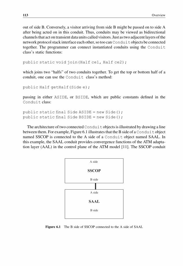
out of side B. Conversely, a visitor arriving from side B might be passed on to side A
after being acted on in this conduit. Thus, conduits may be viewed as bidirectional
channels that act on transient data units called visitors. Just as two adjacent layers of the
network protocol stack interface each other, so too canConduit objects be connected
together. The programmer can connect instantiated conduits using the Conduit
class’s static functions:
public static void join(Half ce1, Half ce2);
which joins two “halfs” of two conduits together. To get the top or bottom half of a
conduit, one can use the Conduit class’s method:
public Half getHalf(Side e);
passing in either ASIDE, or BSIDE, which are public constants defined in the
Conduit class:
public static final Side ASIDE = new Side();
public static final Side BSIDE = new Side();
The architecture of two connectedConduit objects is illustrated by drawing a line
between them. For example, Figure 6.1 illustrates that the B side of aConduit object
named SSCOP is connected to the A side of a Conduit object named SAAL. In
this example, the SAAL conduit provides convergence functions of the ATM adapta-
tion layer (AAL) in the control plane of the ATM model [11]. The SSCOP conduit
A side
SSCOP
B side
A side
SAAL
B side
Figure 6.1 The B side of SSCOP connected to the A side of SAAL
113 Overview
implements the Service Specific Connection Oriented Protocol which provides
reliable transport for ATM control messages.
Example 6.1 illustrates how a programmer can build such a connected group of
conduits.
Example 1: Before connecting the two conduits, theymust be created. The following
abbreviated Java code instantiates and names them:
sscop = new Conduit("SSCOP", sscop protocol);
saal = new Conduit("SAAL", aal protocol);
Then, to connect the B side of SSCOP to the A side of SAAL, the friend functions
are used as follows:
Conduit.join( sscop.getHalf(Conduit.BSIDE),
saal.getHalf(Conduit.ASIDE));
The consequence of the above code is that any visitor leaving out of the A side of
conduit SAALwill be passed into the B side of the SSCOP conduit. Likewise, a visitor
leaving the SSCOPconduit out of its B sidewill enter into the SAALconduit from itsA
side.
Connecting conduits in this manner determines possible communication patterns
between the objects during the application’s lifetime. It should be noted, however, that
the decision of whether to eject a visitor out of a conduit’s A side, or eject it out of the
conduit’s B side, to absorb the visitor, or delay it, rests in the logic of the actual conduit
and visitor. The connectivity of the conduits does not make this decision, rather the
geometric configuration of conduit interconnections only limits the range of possible
outcomes.
The dataflow architecture is the collection of classes that are used to define the
behavior of differentmoduleswithin the protocol stack that is being implemented. The
dataflow architecture is designed to maximize code reuse, make isolation of compo-
nents easy, and render the interactions betweenmodules as transparent as possible.We
will deduce the design of components of CASiNO by considering the needs and
characteristics of applications to be developed using CASiNO. Although the focus is
on the abstract base classes that form the foundation of CASiNO, from time to timewe
comment on the necessary requirements placed on programmers in using this library.
Whenever possible, we will provide details of CASiNO’s internal mechanisms and
code. The CASiNO framework is not very large—it consists of about 350 lines of Java
code, across 15 classes.
Designing and Implementing CASiNO: A Network Simulation Framework 114
Just as data units are processed in each layer of the network protocol stack (e.g.,
segmented, assembled, attached to control information, etc.), a visitor’s passage through
a network of conduits may trigger similar actions. The general manner in which visitors
flow through a conduit is referred to as the conduit’s behavior. Instead of subclassing a
conduit to specialize in the different behaviors, each conduit has a behavior. There are
four derived types of behavior: adapter, mux, factory and protocol, based loosely on the
concepts presented in [10]. Behaviors refer to generic semantic notions: an adapter is a
starting or ending point of a protocol stack; amux is a one-to-many/many-to-one branch
point in a protocol stack; a protocol is a FSM; and a factory is an object capable of
instantiating new conduits and joining them up. Because behaviors represent only
general semantic notions, they must be made concrete by composing them with
appropriate user-defined actors; each behavior has an actor. For example, a protocol
behavior requires a user-defined state machine to be concretely defined. Instances of
conduits, behaviors, and actors are always in one-to-one-to-one correspondence.
To summarize, CASiNO has three tiers in its design:
1. The conduit level of abstraction represents building blocks of the protocol stack; the
function of the Conduit class is to provide a uniform interface for joining these
blocks together and injecting visitors into the resulting networks.
2. The behavior level of abstraction represents broad classes, each capturing different
semantics regarding the conduit’s purpose and activity.
3. Finally, at the actor level of abstraction, the user defines concrete implementations.
Ultimately, CASiNO application programmers must design a suitable actor for
each functionally distinct conduit they intend to instantiate.
As an implementation detail, all conduits, behaviors, and actorsmust be allocated on
the heap. The implicationof this to the programmer is that the “new”operator is used for
creating an actual object of these classes. Deletion of a conduit automatically deletes
any associated Behavior and Actor objects—the destructor of the conduit even-
tually deletes them. Because the objects have identical lifetimes, the relation between
these objects is more of “aggregation” than “acquaintance” or “association [3, p23].”
There are four subclasses of the Actor class: Terminal, Accessor, State,
and Creator. These subclasses of Actor correspond respectively to the subclasses
of Behavior: Adapter, Mux, Protocol, and Factory. There is a relationship
among Conduit, Behavior, and Actor. The one-to-one correspondence among
the instances of conduits, behaviors, and actors is rooted in the belief that a black-box
framework is easier to use, more reusable, and more easily extensible than the “white-
box” framework [10]. A “white-box” approachwould define the four different types of
behaviors as subclass of the Conduit class, while the “black-box” approach lets
Conduit have a reference to these behaviors. A common base class for these four is
defined as class Behavior, and the Conduit class has a reference to a Behavior
115 Overview
object. This is how a one-to-one correspondence betweenConduit andBehavior is
achieved. Regarding the one-to-one correspondence between Behavior and Actor,
the constructor of each subclass of Behavior only takes the appropriate correspond-
ing subclass of theActor object as a parameter. At the conduit level of abstraction, the
basic unit (conduit) is simply an object that can transport visitors. At the behavior level
of abstraction, we identify semantic classes of conduit operation. For example, a mux
operates by multiplexing visitors in one direction and demultiplexing them in another
direction.A terminal is a source/sink of visitors.A factory is a placewhere new conduits
are made. To fully specify a concrete behavior several details must be specified: for
example, for amux, “how does amux determinewhere to demultiplex a visitor to?”; for
a factory, “what kind of conduit should bemade?”; and so on. This specification process
could have been carried out in twoways: (1) by making certain methods abstract in the
behavior hierarchy and then requiring concrete versions of the behaviors to implement
these abstract methods; or (2) by composition of the specification into the behavior. We
chose the latter approach, and we call the specification objects actors. If we consider
CASiNOas a high-level language, the set of behaviors is in essence the syntactic classes
of the language, whereas the set of actors consists of the concrete words within the
syntactic classes. We wanted to make the act of extending syntactic classes different
from the action of implementing new concretewordswithin a syntactic class. The latter
is commonplace in designing a CASiNO application; the former constitutes extending
the CASiNO framework. Conduits receive and are given visitors through their
acceptVisitorFrom() method. The code below, for example, sends the visitor
v to the conduit C:
Visitor v = new PacketVisitor(0, 111);
Conduit C = new Conduit("MyConduit", my protocol);
C.acceptVisitorFrom(v, Conduit.ASIDE);
Visitorsmay be thought of as transient objects, usually representing communication
messages or dataflow. However, because visitors are full Java objects they are much
more than just passive data packets or “buffers.”. A visitor is a smart object, with the
potential of having its own logic and interacting with the logic of user-defined actors.
So at each conduit, a dialog between thevisitor and the underlying actor ensues, and the
outcome of this dialog determines the side effects within the state of the visitor and the
state of the actor. Precisely, the visitor is first informed of the conduit where it is about
to find itself situated. This is done by calling the visitor’s arrivedAt() method:
void arrivedAt(Conduit.Half ce);
This method may optionally be redefined within the application’s derived visitors;
in the default implementation, the visitor merely adds to its internal log of conduits it
Designing and Implementing CASiNO: A Network Simulation Framework 116

has visited. This log can later be revealed, analyzed, and if necessary cleared.
Programmers who use CASiNO must derive all of their visitors from the abstract
base class Visitor. All visitors must be allocated on the heap. Destruction of a
visitor takes place by garbage collection when no reachable references exist:
1. When making a conduit, the programmer is required to specify its behavior. As
mentioned earlier, there are four types of behaviors, each representing general
semantics of a conduit’s purpose and activity:
(a) Protocol behavior: Contains the logic for a FSM.
(b) Adapter behavior: Absorbs and/or generates new visitors; interfaces with
non-framework software.
(c) Muxbehavior: Demultiplexes visitors to (andmultiplexes visitors from) a set
of adjacent conduits.
(d) Factory behavior: Creates and attaches new conduits to neighboring muxes.
2. The programmer must fully specify a behavior at the time of construction with an
appropriate concrete Actor object. There are, correspondingly, four types of
actors:
(a) State actor: Required to specify a protocol.
(b) Terminal actor: Required to specify an adapter.
(c) Accessor actor: Required to specify a mux.
(d) Creator actor: Required to specify a factory.
Now that we have a rough outline of how we see the framework operating, let us
proceed by defining the Conduit and Visitor classes. Once that is done, we will
proceed with the Behavior classes and the corresponding Actor interfaces.
6.2 Conduits
Closely associatedwith a conduit is the notion of a “side.” Every conduit has two sides,
whichwe refer to as theASIDE (“A” for above) and theBSIDE (“B” for below). Thus,
inside the Conduit class:
public final class Conduit {
}
we will have a static class called Side:
public static class Side {};
public static final Side ASIDE = new Side();
public static final Side BSIDE = new Side();
117 Conduits
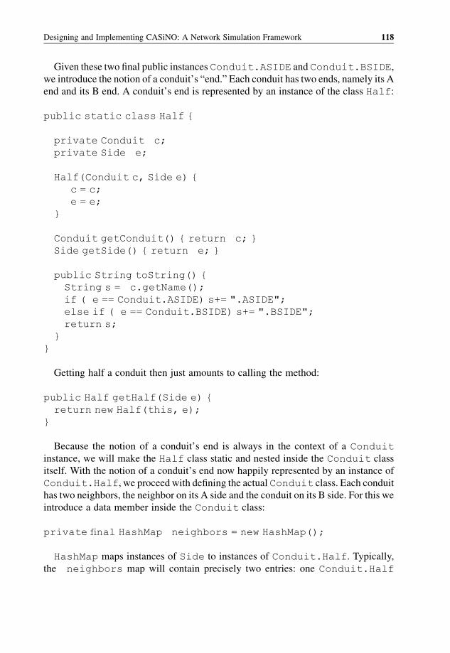
Given these two final public instances Conduit.ASIDE and Conduit.BSIDE,
we introduce the notion of a conduit’s “end.” Each conduit has two ends, namely its A
end and its B end. A conduit’s end is represented by an instance of the class Half:
public static class Half {
private Conduit c;
private Side e;
Half(Conduit c, Side e) {
c = c;
e = e;
}
Conduit getConduit() { return c; }
Side getSide() { return e; }
public String toString() {
String s = c.getName();
if ( e == Conduit.ASIDE) s+= ".ASIDE";
else if ( e == Conduit.BSIDE) s+= ".BSIDE";
return s;
}
}
Getting half a conduit then just amounts to calling the method:
public Half getHalf(Side e) {
return new Half(this, e);
}
Because the notion of a conduit’s end is always in the context of a Conduit
instance, we will make the Half class static and nested inside the Conduit class
itself. With the notion of a conduit’s end now happily represented by an instance of
Conduit.Half, we proceed with defining the actual Conduit class. Each conduit
has two neighbors, the neighbor on its A side and the conduit on its B side. For this we
introduce a data member inside the Conduit class:
private final HashMap neighbors = new HashMap();
HashMap maps instances of Side to instances of Conduit.Half. Typically,
the neighbors map will contain precisely two entries: one Conduit.Half
Designing and Implementing CASiNO: A Network Simulation Framework 118
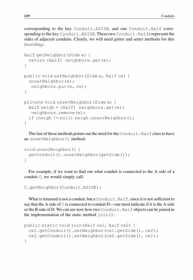
corresponding to the key Conduit.ASIDE, and one Conduit.Half corre-
sponding to the key Conduit.BSIDE. These two Conduit.Halfs represent the
sides of adjacent conduits. Clearly, we will need getter and setter methods for this
HashMap:
Half getNeighbor(Side e) {
return (Half) neighbors.get(e);
}
public void setNeighbor(Side e, Half ce) {
unsetNeighbor(e);
neighbors.put(e, ce);
}
private void unsetNeighbor(Side e) {
Half neigh = (Half) neighbors.get(e);
neighbors.remove(e);
if (neigh != null) neigh.unsetNeighbor();
}
The last of thesemethods points out the need for theConduit.Half class to have
an unsetNeighbor() method:
void unsetNeighbor() {
getConduit().unsetNeighbor(getSide());
}
For example, if we want to find out what conduit is connected to the A side of a
conduit C, we would simply call:
C.getNeighbor(Conduit.ASIDE);
What is returned is not a conduit, but a Conduit.Half, since it is not sufficient to
say that the A side of C is connected to conduit D—one must indicate if it is the A side
or the B side of D.We can see now how two Conduit.Half objects can be joined in
the implementation of the static method join():
public static void join(Half ce1, Half ce2) {
ce1.getConduit().setNeighbor(ce1.getSide(), ce2);
ce2.getConduit().setNeighbor(ce2.getSide(), ce1);
}
119 Conduits
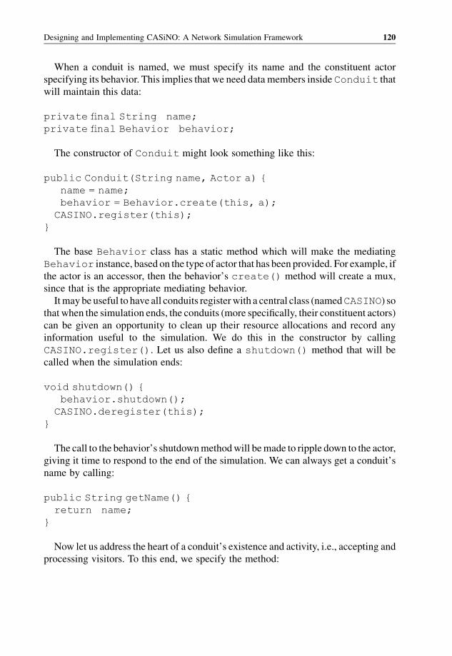
When a conduit is named, we must specify its name and the constituent actor
specifying its behavior. This implies that we need data members inside Conduit that
will maintain this data:
private final String name;
private final Behavior behavior;
The constructor of Conduit might look something like this:
public Conduit(String name, Actor a) {
name = name;
behavior = Behavior.create(this, a);
CASINO.register(this);
}
The base Behavior class has a static method which will make the mediating
Behavior instance, based on the type of actor that has been provided. For example, if
the actor is an accessor, then the behavior’s create() method will create a mux,
since that is the appropriate mediating behavior.
Itmay be useful to have all conduits registerwith a central class (namedCASINO) so
that when the simulation ends, the conduits (more specifically, their constituent actors)
can be given an opportunity to clean up their resource allocations and record any
information useful to the simulation. We do this in the constructor by calling
CASINO.register(). Let us also define a shutdown() method that will be
called when the simulation ends:
void shutdown() {
behavior.shutdown();
CASINO.deregister(this);
}
The call to the behavior’s shutdownmethodwill bemade to ripple down to the actor,
giving it time to respond to the end of the simulation. We can always get a conduit’s
name by calling:
public String getName() {
return name;
}
Now let us address the heart of a conduit’s existence and activity, i.e., accepting and
processing visitors. To this end, we specify the method:
Designing and Implementing CASiNO: A Network Simulation Framework 120
public void acceptVisitorFrom(Visitor v, Side e) {
Half route = behavior.acceptVisitorFrom(v,e);
if (route != null) {
route.acceptVisitor(v);
}
}
The call to the behavior’sacceptmethodencompasses the conduit’s local response
to the arrival of the visitor. The return value of this method call is the place to which
the visitor must be routed to next. Notice that the conduit delegates to the behavior the
decision about where to send the visitor next. The behavior will in turn delegate to
the actor—but the nature of this second delegation depends on the specific type of the
behavior. The outcome of this double delegation is a determination of where the visitor
should go next. The conduit forwards the visitor to the determined destination route,
which is the nextConduit.Half towhich thevisitormust be sent. This points out the
need for the Conduit.Half class having an acceptVisitor() method:
void acceptVisitor(Visitor v) {
v.arrivedAt(this);
getConduit().acceptVisitorFrom(v, getSide());
}
Note that before making the conduit accept the visitor via its acceptVisitor
From() method, we notify the visitor that it has arrived at a specific Conduit.
Half. One final utility method will prove useful, and we define it statically in the
Conduit class:
static Side otherSide(Side e) {
if (e==ASIDE) return BSIDE;
else return ASIDE;
}
This method may be needed to determine “pass-through” behavior—that is, if a
visitor came in through the A side, which side should it go out through “usually?” The
other side from where it entered. We have now completed the specification of the
Conduit class. Let us turn now to visitors.
6.3 Visitors
We know that visitors are the transient elements that flow through conduits. The
decisions about how to respond to visitors and where to route them next are
121 Visitors
determined by behaviors, and ultimately by the actors specifying them. So far, in
Conduit, the only time that a visitor’s methods are called is in Conduit.
Half’s accept() method, which informs the visitor of its impending arrival
prior to handing the visitor off to the conduit. It follows that we must define the
arrivedAt() method for Visitor—but what do we put in it? In the base
implementation of Visitor, we simply keep a log of the conduit names that the
visitor has arrived at. This log can be used later for diagnostics and simulation
analysis and visualization. Below then is the complete code for the base Visitor
class:
public class Visitor {
void arrivedAt(Conduit.Half ce) {
log.addLast(ce.toString());
}
private final LinkedList log = new LinkedList();
public void clearLog() {
log.clear();
}
public String getLog() {
String s = "";
for (Iterator it= log.iterator(); it.hasNext();) {
String s1 = (String)it.next();
s += s1;
}
return s;
}
}
The getLog() and clearLog() methods allow external classes to get the log
from a visitor, or to zero-out its contents.
6.4 The Conduit Repository
In defining the Conduit class, we noted that we need to have a central repository of
conduits so that when the simulation ends, all conduits can be given an opportunity to
report their results and return system resources to an appropriate state. This central
repository is maintained in the CASINO class:
Designing and Implementing CASiNO: A Network Simulation Framework 122
public final class CASINO {
static final HashSet conduits = new HashSet();
static void register(Conduit c) {
conduits.add(c);
}
static void deregister(Conduit c) {
conduits.remove(c);
}
public static void shutdown() {
while ( conduits.size() > 0) {
Iterator it = conduits.iterator();
Conduit c = (Conduit)it.next();
c.shutdown();
}
}
}
Calling CASINO.shutdown at the end of the simulation would result in every
conduit having its shutdown method being called, sequentially.
6.5 Behaviors and Actors
Recall that behaviors are made in the conduit’s constructor by calling the static
Behavior.create() method, which is supposed to make the appropriate medi-
ating behavior correspond to the type of actor provided. This naturally suggests that
the Behavior class should have a method like:
static Behavior create(Conduit c, Actor a) {
Behavior b = null;
if (a instanceof Terminal) b = new Adapter(c, (Terminal)a);
if (a instanceof State) b = new Protocol(c, (State)a);
if (a instanceof Accessor) b = new Mux(c, (Accessor)a);
if (a instanceof Creator) b = new Factory(c, (Creator)a);
return b;
}
Since it is likely that all behaviors will need a reference to their ambient conduit (so
that they can understand the geometry of their relationships with their neighbors), it
123 Behaviors and Actors
would be a good idea to have a protected data member:
protected Conduit c;
in Behavior, and require that this be specified in the constructor:
protected Behavior(Conduit c) {
c = c;
}
Since behaviors cannot be made without reference to a conduit, they can have a
notion of name that is inherited from the conduit:
public String getName() {
return c.getName();
}
Every behavior is responsible for responding to the arrival of visitors (by delegation
to an actor), as well as determining the next destination conduit for the visitor. To this
end, it will be helpful to define the notion of a “default” route for the visitor: by default
thevisitorwill be sent to the conduitwhich is connected to the “other” side—that is, if it
came in from theA side, then itwill by default be sent to the conduit that is connected to
the B side:
public final Conduit.Half defaultRoute(Conduit.Side e) {
return c.getNeighbor(Conduit.otherSide(e));
}
Finally, there are many different classes of behaviors, and each of these will
have a different notion of how to accept a visitor, what to do with it, and how to
determine where to send it next. It follows that in the Behavior class, the
method:
abstract Conduit.Half acceptVisitorFrom(Visitor v,
Conduit.Side e);
must be abstract. Similarly, since the actions of each Behavior subclass are
different, how each of the concrete behaviors “shut down” at the end of the simulation
is also likely to be quite different. Accordingly, we define:
abstract void shutdown();
Designing and Implementing CASiNO: A Network Simulation Framework 124
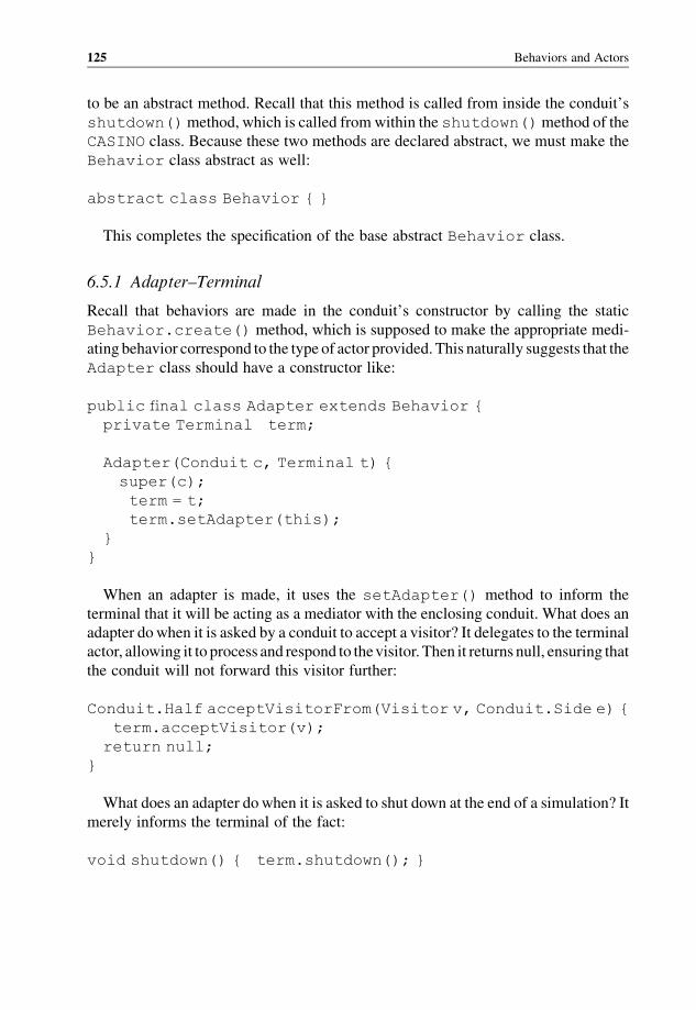
to be an abstract method. Recall that this method is called from inside the conduit’s
shutdown()method, which is called from within the shutdown()method of the
CASINO class. Because these two methods are declared abstract, we must make the
Behavior class abstract as well:
abstract class Behavior { }
This completes the specification of the base abstract Behavior class.
6.5.1 Adapter–Terminal
Recall that behaviors are made in the conduit’s constructor by calling the static
Behavior.create() method, which is supposed to make the appropriate medi-
ating behavior correspond to the type of actor provided. This naturally suggests that the
Adapter class should have a constructor like:
public final class Adapter extends Behavior {
private Terminal term;
Adapter(Conduit c, Terminal t) {
super(c);
term = t;
term.setAdapter(this);
}
}
When an adapter is made, it uses the setAdapter() method to inform the
terminal that it will be acting as a mediator with the enclosing conduit. What does an
adapter dowhen it is asked by a conduit to accept a visitor? It delegates to the terminal
actor, allowing it to process and respond to thevisitor. Then it returns null, ensuring that
the conduit will not forward this visitor further:
Conduit.Half acceptVisitorFrom(Visitor v, Conduit.Side e) {
term.acceptVisitor(v);
return null;
}
What does an adapter do when it is asked to shut down at the end of a simulation? It
merely informs the terminal of the fact:
void shutdown() { term.shutdown(); }
125 Behaviors and Actors
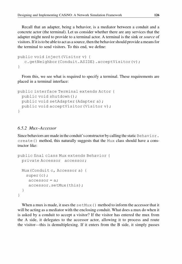
Recall that an adapter, being a behavior, is a mediator between a conduit and a
concrete actor (the terminal). Let us consider whether there are any services that the
adapter might need to provide to a terminal actor. A terminal is the sink or source of
visitors. If it is to be able to act as a source, then the behavior should provide ameans for
the terminal to send visitors. To this end, we define:
public void inject(Visitor v) {
c.getNeighbor(Conduit.ASIDE).acceptVisitor(v);
}
From this, we see what is required to specify a terminal. These requirements are
placed in a terminal interface:
public interface Terminal extends Actor {
public void shutdown();
public void setAdapter(Adapter a);
public void acceptVisitor(Visitor v);
}
6.5.2 Mux–Accessor
Since behaviors aremade in the conduit’s constructor by calling the staticBehavior.
create() method, this naturally suggests that the Mux class should have a cons-
tructor like:
public final class Mux extends Behavior {
private Accessor accessor;
Mux(Conduit c, Accessor a) {
super(c);
accessor = a;
accessor.setMux(this);
}
}
When a mux is made, it uses the setMux()method to inform the accessor that it
will be acting as a mediator with the enclosing conduit. What does a mux do when it
is asked by a conduit to accept a visitor? If the visitor has entered the mux from
the A side, it delegates to the accessor actor, allowing it to process and route
the visitor—this is demultiplexing. If it enters from the B side, it simply passes
Designing and Implementing CASiNO: A Network Simulation Framework 126
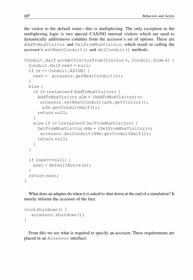
the visitor to the default route—this is multiplexing. The only exception to the
multiplexing logic is two special CASiNO internal visitors which are used to
dynamically add/remove conduits from the accessor’s set of options. These are
AddToMuxVisitor and DelFromMuxVisitor, which result in calling the
accessor’s setNextConduit() and delConduit() methods:
Conduit.Half acceptVisitorFrom(Visitor v, Conduit.Side e) {
Conduit.Half next = null;
if (e == Conduit.ASIDE) {
next = accessor.getNextConduit(v);
}
else {
if (v instanceof AddToMuxVisitor) {
AddToMuxVisitor a2m = (AddToMuxVisitor)v;
accessor.setNextConduit(a2m.getVisitor(),
a2m.getConduitHalf());
return null;
}
else if (v instanceof DelFromMuxVisitor) {
DelFromMuxVisitor d4m = (DelFromMuxVisitor)v;
accessor.delConduit(d4m.getConduitHalf());
return null;
}
}
if (next==null) {
next = defaultRoute(e);
}
return next;
}
What does an adapter do when it is asked to shut down at the end of a simulation? It
merely informs the accessor of the fact:
void shutdown() {
accessor.shutdown();
}
From this we see what is required to specify an accessor. These requirements are
placed in an Accessor interface:
127 Behaviors and Actors
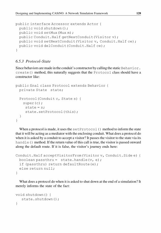
public interface Accessor extends Actor {
public void shutdown();
public void setMux(Mux m);
public Conduit.Half getNextConduit(Visitor v);
public void setNextConduit(Visitor v, Conduit.Half ce);
public void delConduit(Conduit.Half ce);
}
6.5.3 Protocol–State
Since behaviors aremade in the conduit’s constructor by calling the staticBehavior.
create() method, this naturally suggests that the Protocol class should have a
constructor like:
public final class Protocol extends Behavior {
private State state;
Protocol(Conduit c, State s) {
super(c);
state = s;
state.setProtocol(this);
}
}
When a protocol is made, it uses the setProtocol()method to inform the state
that it will be acting as a mediator with the enclosing conduit. What does a protocol do
when it is asked by a conduit to accept a visitor? It passes the visitor to the state via its
handle()method. If the return value of this call is true, the visitor is passed onward
along the default route. If it is false, the visitor’s journey ends here:
Conduit.Half acceptVisitorFrom(Visitor v, Conduit.Side e) {
boolean passthru = state.handle(v, e);
if (passthru) return defaultRoute(e);
else return null;
}
What does a protocol do when it is asked to shut down at the end of a simulation? It
merely informs the state of the fact:
void shutdown() {
state.shutdown();
}
Designing and Implementing CASiNO: A Network Simulation Framework 128
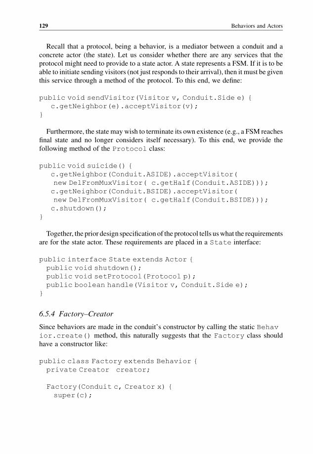
Recall that a protocol, being a behavior, is a mediator between a conduit and a
concrete actor (the state). Let us consider whether there are any services that the
protocol might need to provide to a state actor. A state represents a FSM. If it is to be
able to initiate sending visitors (not just responds to their arrival), then it must be given
this service through a method of the protocol. To this end, we define:
public void sendVisitor(Visitor v, Conduit.Side e) {
c.getNeighbor(e).acceptVisitor(v);
}
Furthermore, the state may wish to terminate its own existence (e.g., a FSM reaches
final state and no longer considers itself necessary). To this end, we provide the
following method of the Protocol class:
public void suicide() {
c.getNeighbor(Conduit.ASIDE).acceptVisitor(
new DelFromMuxVisitor( c.getHalf(Conduit.ASIDE)));
c.getNeighbor(Conduit.BSIDE).acceptVisitor(
new DelFromMuxVisitor( c.getHalf(Conduit.BSIDE)));
c.shutdown();
}
Together, the prior design specification of the protocol tells uswhat the requirements
are for the state actor. These requirements are placed in a State interface:
public interface State extends Actor {
public void shutdown();
public void setProtocol(Protocol p);
public boolean handle(Visitor v, Conduit.Side e);
}
6.5.4 Factory–Creator
Since behaviors are made in the conduit’s constructor by calling the static Behav
ior.create() method, this naturally suggests that the Factory class should
have a constructor like:
public class Factory extends Behavior {
private Creator creator;
Factory(Conduit c, Creator x) {
super(c);
129 Behaviors and Actors
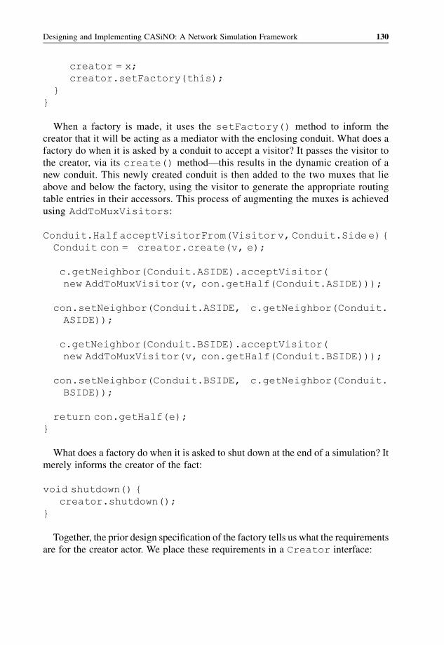
creator = x;
creator.setFactory(this);
}
}
When a factory is made, it uses the setFactory() method to inform the
creator that it will be acting as a mediator with the enclosing conduit. What does a
factory do when it is asked by a conduit to accept a visitor? It passes the visitor to
the creator, via its create() method—this results in the dynamic creation of a
new conduit. This newly created conduit is then added to the two muxes that lie
above and below the factory, using the visitor to generate the appropriate routing
table entries in their accessors. This process of augmenting the muxes is achieved
using AddToMuxVisitors:
Conduit.HalfacceptVisitorFrom(Visitorv,Conduit.Sidee){
Conduit con = creator.create(v, e);
c.getNeighbor(Conduit.ASIDE).acceptVisitor(
new AddToMuxVisitor(v, con.getHalf(Conduit.ASIDE)));
con.setNeighbor(Conduit.ASIDE, c.getNeighbor(Conduit.
ASIDE));
c.getNeighbor(Conduit.BSIDE).acceptVisitor(
new AddToMuxVisitor(v, con.getHalf(Conduit.BSIDE)));
con.setNeighbor(Conduit.BSIDE, c.getNeighbor(Conduit.
BSIDE));
return con.getHalf(e);
}
What does a factory do when it is asked to shut down at the end of a simulation? It
merely informs the creator of the fact:
void shutdown() {
creator.shutdown();
}
Together, the prior design specification of the factory tells us what the requirements
are for the creator actor. We place these requirements in a Creator interface:
Designing and Implementing CASiNO: A Network Simulation Framework 130
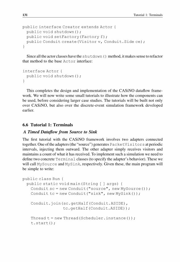
public interface Creator extends Actor {
public void shutdown();
public void setFactory(Factory f);
public Conduit create(Visitor v, Conduit.Side ce);
}
Since all the actor classes have theshutdown()method, itmakes sense to refactor
that method to the base Actor interface:
interface Actor {
public void shutdown();
}
This completes the design and implementation of the CASiNO dataflow frame-
work. We will now write some small tutorials to illustrate how the components can
be used, before considering larger case studies. The tutorials will be built not only
over CASiNO, but also over the discrete-event simulation framework developed
earlier.
6.6 Tutorial 1: Terminals
A Timed Dataflow from Source to Sink
The first tutorial with the CASiNO framework involves two adapters connected
together. One of the adapters (the “source”) generatesPacketVisitors at periodic
intervals, injecting them outward. The other adapter simply receives visitors and
maintains a count of what it has received. To implement such a simulation we need to
define two concrete Terminal classes (to specify the adapter’s behavior). These we
will call MySource and MySink, respectively. Given these, the main program will
be simple to write:
public class Run {
public static void main(String [ ] args) {
Conduit sc = new Conduit("source", new MySource());
Conduit tc = new Conduit("sink", new MySink());
Conduit.join(sc.getHalf(Conduit.ASIDE),
tc.getHalf(Conduit.ASIDE));
Thread t = new Thread(Scheduler.instance());
t.start();
131 Tutorial 1: Terminals
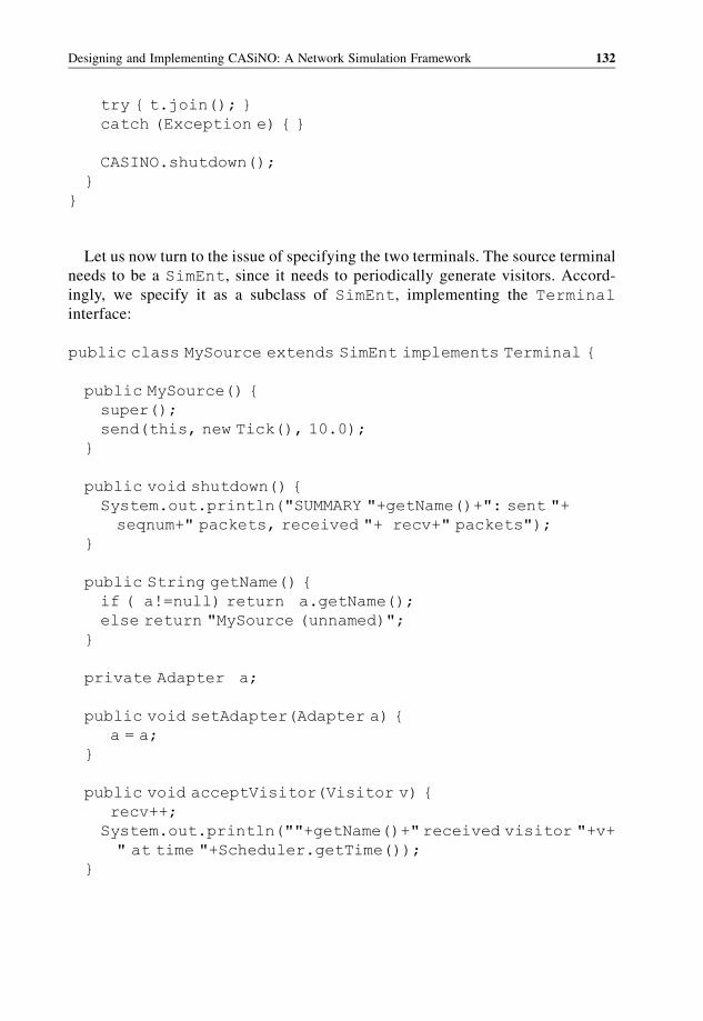
try { t.join(); }
catch (Exception e) { }
CASINO.shutdown();
}
}
Let us now turn to the issue of specifying the two terminals. The source terminal
needs to be a SimEnt, since it needs to periodically generate visitors. Accord-
ingly, we specify it as a subclass of SimEnt, implementing the Terminal
interface:
public class MySource extends SimEnt implements Terminal {
public MySource() {
super();
send(this, new Tick(), 10.0);
}
public void shutdown() {
System.out.println("SUMMARY "+getName()+": sent "+
seqnum+" packets, received "+ recv+" packets");
}
public String getName() {
if ( a!=null) return a.getName();
else return "MySource (unnamed)";
}
private Adapter a;
public void setAdapter(Adapter a) {
a = a;
}
public void acceptVisitor(Visitor v) {
recv++;
System.out.println(""+getName()+"received visitor "+v+
" at time "+Scheduler.getTime());
}
Designing and Implementing CASiNO: A Network Simulation Framework 132
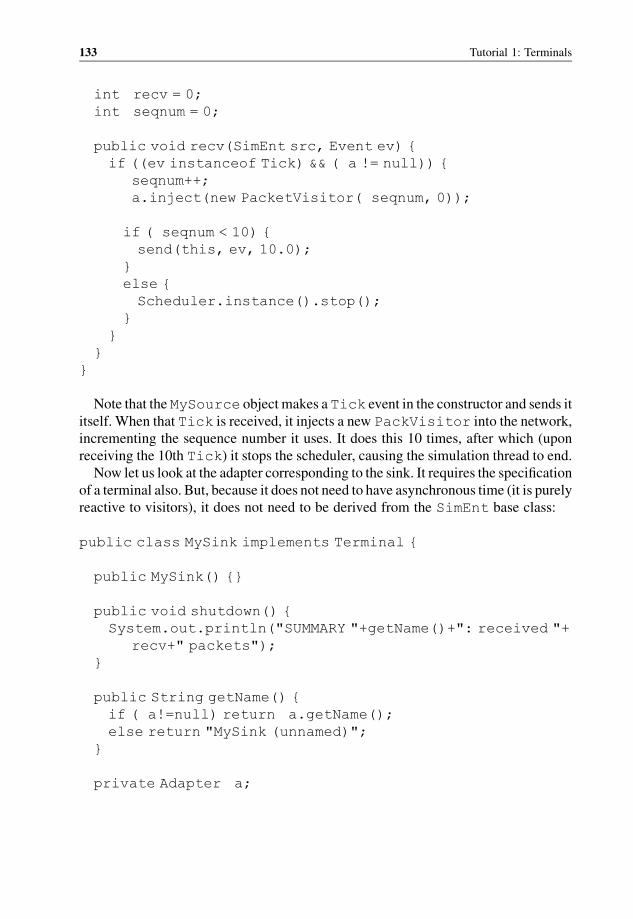
int recv = 0;
int seqnum = 0;
public void recv(SimEnt src, Event ev) {
if ((ev instanceof Tick) && ( a != null)) {
seqnum++;
a.inject(new PacketVisitor( seqnum, 0));
if ( seqnum < 10) {
send(this, ev, 10.0);
}
else {
Scheduler.instance().stop();
}
}
}
}
Note that the MySource object makes a Tick event in the constructor and sends it
itself. When that Tick is received, it injects a new PackVisitor into the network,
incrementing the sequence number it uses. It does this 10 times, after which (upon
receiving the 10th Tick) it stops the scheduler, causing the simulation thread to end.
Now let us look at the adapter corresponding to the sink. It requires the specification
of a terminal also. But, because it does not need to have asynchronous time (it is purely
reactive to visitors), it does not need to be derived from the SimEnt base class:
public class MySink implements Terminal {
public MySink() {}
public void shutdown() {
System.out.println("SUMMARY "+getName()+": received "+
recv+" packets");
}
public String getName() {
if ( a!=null) return a.getName();
else return "MySink (unnamed)";
}
private Adapter a;
133 Tutorial 1: Terminals
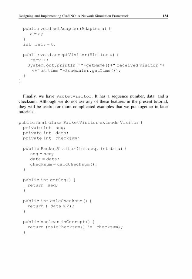
public void setAdapter(Adapter a) {
a = a;
}
int recv = 0;
public void acceptVisitor(Visitor v) {
recv++;
System.out.println(""+getName()+" received visitor "+
v+" at time "+Scheduler.getTime());
}
}
Finally, we have PacketVisitor. It has a sequence number, data, and a
checksum. Although we do not use any of these features in the present tutorial,
they will be useful for more complicated examples that we put together in later
tutorials.
public final class PacketVisitor extends Visitor {
private int seq;
private int data;
private int checksum;
public PacketVisitor(int seq, int data) {
seq = seq;
data = data;
checksum = calcChecksum();
}
public int getSeq() {
return seq;
}
public int calcChecksum() {
return ( data % 2);
}
public boolean isCorrupt() {
return (calcChecksum() != checksum);
}
Designing and Implementing CASiNO: A Network Simulation Framework 134
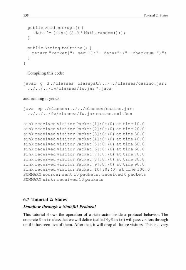
public void corrupt() {
data ^= ((int)(2.0 * Math.random()));
}
public String toString() {
return "Packet["+ seq+"]:"+ data+":("+ checksum+")";
}
}
Compiling this code:
javac g d ./classes classpath ../../classes/casino.jar:
../../../fw/classes/fw.jar *.java
and running it yields:
java cp ./classes:../../classes/casino.jar:
../../../fw/classes/fw.jar casino.ex1.Run
sink received visitor Packet[1]:0:(0) at time 10.0
sink received visitor Packet[2]:0:(0) at time 20.0
sink received visitor Packet[3]:0:(0) at time 30.0
sink received visitor Packet[4]:0:(0) at time 40.0
sink received visitor Packet[5]:0:(0) at time 50.0
sink received visitor Packet[6]:0:(0) at time 60.0
sink received visitor Packet[7]:0:(0) at time 70.0
sink received visitor Packet[8]:0:(0) at time 80.0
sink received visitor Packet[9]:0:(0) at time 90.0
sink received visitor Packet[10]:0:(0) at time 100.0
SUMMARY source: sent 10 packets, received 0 packets
SUMMARY sink: received 10 packets
6.7 Tutorial 2: States
Dataflow through a Stateful Protocol
This tutorial shows the operation of a state actor inside a protocol behavior. The
concrete State class that wewill define (called MyState) will pass visitors through
until it has seen five of them. After that, it will drop all future visitors. This is a very
135 Tutorial 2: States
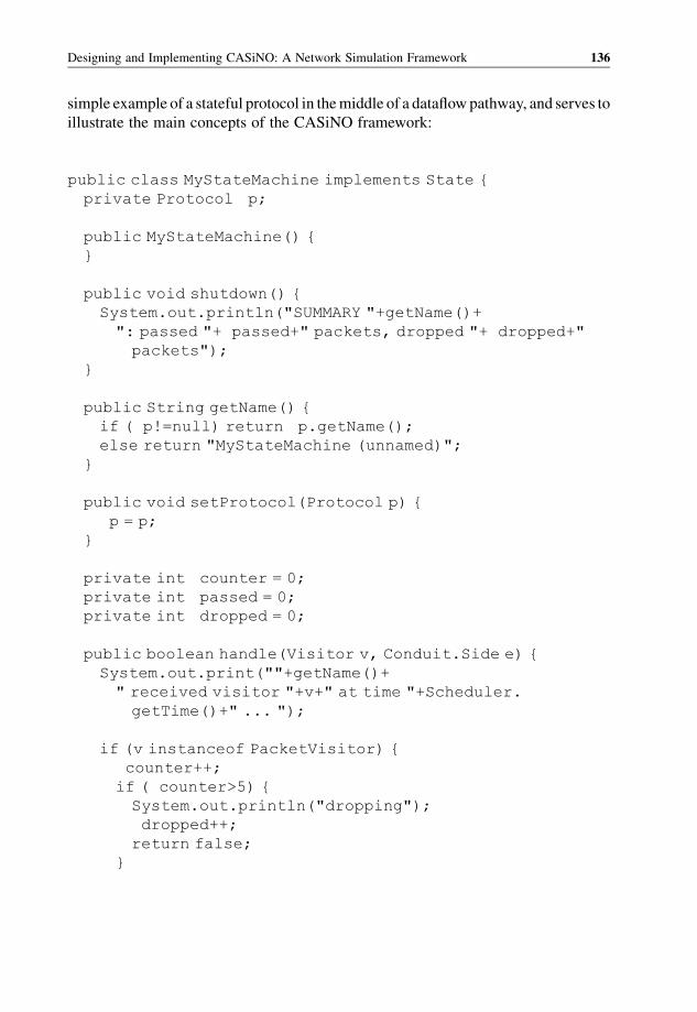
simple example of a stateful protocol in themiddle of a dataflowpathway, and serves to
illustrate the main concepts of the CASiNO framework:
public class MyStateMachine implements State {
private Protocol p;
public MyStateMachine() {
}
public void shutdown() {
System.out.println("SUMMARY "+getName()+
": passed "+ passed+" packets, dropped "+ dropped+"
packets");
}
public String getName() {
if ( p!=null) return p.getName();
else return "MyStateMachine (unnamed)";
}
public void setProtocol(Protocol p) {
p = p;
}
private int counter = 0;
private int passed = 0;
private int dropped = 0;
public boolean handle(Visitor v, Conduit.Side e) {
System.out.print(""+getName()+
" received visitor "+v+" at time "+Scheduler.
getTime()+" ... ");
if (v instanceof PacketVisitor) {
counter++;
if ( counter>5) {
System.out.println("dropping");
dropped++;
return false;
}
Designing and Implementing CASiNO: A Network Simulation Framework 136

else {
System.out.println("passing through");
passed++;
return true;
}
}
else return true;
}
}
The new state is used to populate a protocol behavior in a conduit which lies
in between the two terminals (a MySource and a MySink). The resulting main()
function is only a slight extension of what was written for Tutorial 1:
public class Run {
public static void main(String [ ] args) {
Conduit sc = new Conduit("source", new MySource());
Conduit mc = new Conduit("fsm", new MyStateMachine());
Conduit tc = new Conduit("sink", new MySink());
Conduit.join(sc.getHalf(Conduit.ASIDE),
mc.getHalf(Conduit.ASIDE));
Conduit.join(mc.getHalf(Conduit.BSIDE),
tc.getHalf(Conduit.ASIDE));
Thread t = new Thread(Scheduler.instance());
t.start();
try { t.join(); }
catch (Exception e) { }
CASINO.shutdown();
}
}
We can now compile the second example and run it:
javac g d
./classes classpath
../../classes/casino.jar:../../../fw/classes/fw.jar:
../ex1/classes *.java
137 Tutorial 2: States
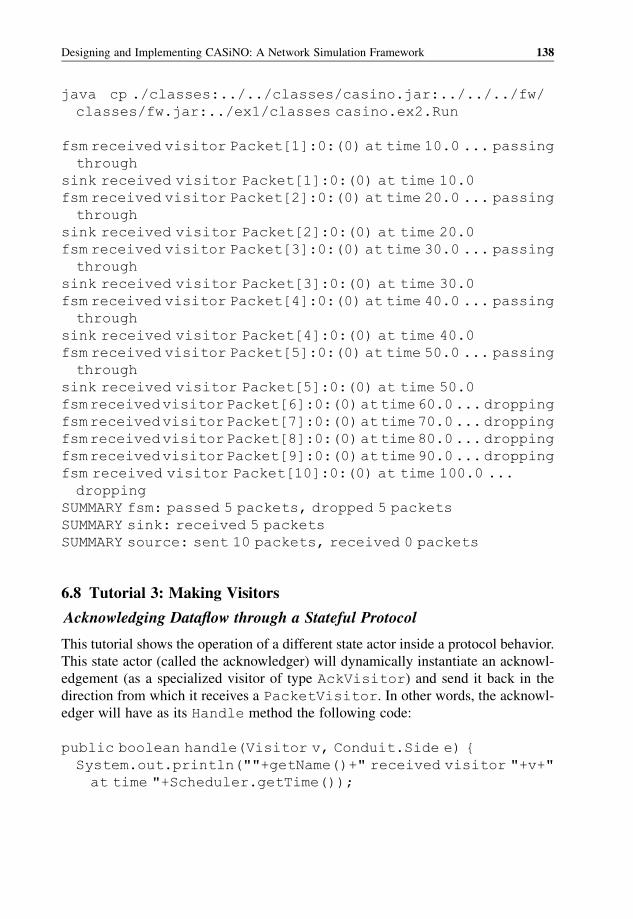
java cp ./classes:../../classes/casino.jar:../../../fw/
classes/fw.jar:../ex1/classes casino.ex2.Run
fsm received visitor Packet[1]:0:(0) at time 10.0 ... passing
through
sink received visitor Packet[1]:0:(0) at time 10.0
fsm received visitor Packet[2]:0:(0) at time 20.0 ... passing
through
sink received visitor Packet[2]:0:(0) at time 20.0
fsm received visitor Packet[3]:0:(0) at time 30.0 ... passing
through
sink received visitor Packet[3]:0:(0) at time 30.0
fsm received visitor Packet[4]:0:(0) at time 40.0 ... passing
through
sink received visitor Packet[4]:0:(0) at time 40.0
fsm received visitor Packet[5]:0:(0) at time 50.0 ... passing
through
sink received visitor Packet[5]:0:(0) at time 50.0
fsmreceivedvisitorPacket[6]:0:(0)attime60.0...dropping
fsmreceivedvisitorPacket[7]:0:(0)attime70.0...dropping
fsmreceivedvisitorPacket[8]:0:(0)attime80.0...dropping
fsmreceivedvisitorPacket[9]:0:(0)attime90.0...dropping
fsm received visitor Packet[10]:0:(0) at time 100.0 ...
dropping
SUMMARY fsm: passed 5 packets, dropped 5 packets
SUMMARY sink: received 5 packets
SUMMARY source: sent 10 packets, received 0 packets
6.8 Tutorial 3: Making Visitors
Acknowledging Dataflow through a Stateful Protocol
This tutorial shows the operation of a different state actor inside a protocol behavior.
This state actor (called the acknowledger) will dynamically instantiate an acknowl-
edgement (as a specialized visitor of type AckVisitor) and send it back in the
direction from which it receives a PacketVisitor. In other words, the acknowl-
edger will have as its Handle method the following code:
public boolean handle(Visitor v, Conduit.Side e) {
System.out.println(""+getName()+" received visitor "+v+"
at time "+Scheduler.getTime());
Designing and Implementing CASiNO: A Network Simulation Framework 138
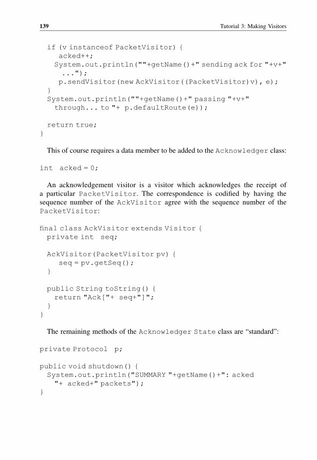
if (v instanceof PacketVisitor) {
acked++;
System.out.println(""+getName()+" sending ack for "+v+"
...");
p.sendVisitor(new AckVisitor((PacketVisitor)v), e);
}
System.out.println(""+getName()+" passing "+v+"
through... to "+ p.defaultRoute(e));
return true;
}
This of course requires a data member to be added to the Acknowledger class:
int acked = 0;
An acknowledgement visitor is a visitor which acknowledges the receipt of
a particular PacketVisitor. The correspondence is codified by having the
sequence number of the AckVisitor agree with the sequence number of the
PacketVisitor:
final class AckVisitor extends Visitor {
private int seq;
AckVisitor(PacketVisitor pv) {
seq = pv.getSeq();
}
public String toString() {
return "Ack["+ seq+"]";
}
}
The remaining methods of the Acknowledger State class are “standard”:
private Protocol p;
public void shutdown() {
System.out.println("SUMMARY "+getName()+": acked
"+ acked+" packets");
}
139 Tutorial 3: Making Visitors
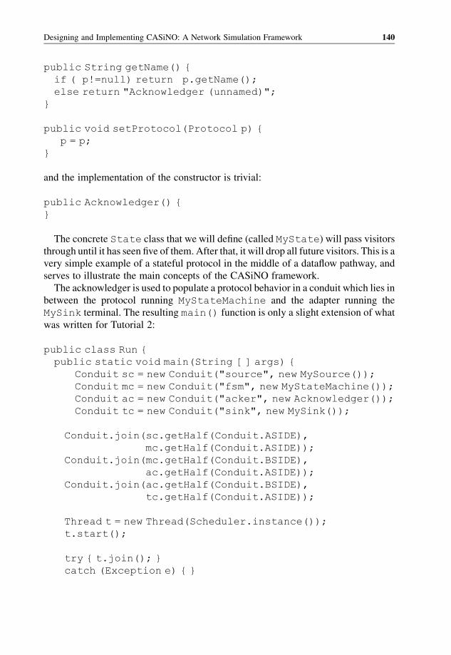
public String getName() {
if ( p!=null) return p.getName();
else return "Acknowledger (unnamed)";
}
public void setProtocol(Protocol p) {
p = p;
}
and the implementation of the constructor is trivial:
public Acknowledger() {
}
The concrete State class that we will define (called MyState) will pass visitors
through until it has seen five of them. After that, it will drop all future visitors. This is a
very simple example of a stateful protocol in the middle of a dataflow pathway, and
serves to illustrate the main concepts of the CASiNO framework.
The acknowledger is used to populate a protocol behavior in a conduit which lies in
between the protocol running MyStateMachine and the adapter running the
MySink terminal. The resulting main() function is only a slight extension of what
was written for Tutorial 2:
public class Run {
public static void main(String [ ] args) {
Conduit sc = new Conduit("source", new MySource());
Conduit mc = new Conduit("fsm", new MyStateMachine());
Conduit ac = new Conduit("acker", new Acknowledger());
Conduit tc = new Conduit("sink", new MySink());
Conduit.join(sc.getHalf(Conduit.ASIDE),
mc.getHalf(Conduit.ASIDE));
Conduit.join(mc.getHalf(Conduit.BSIDE),
ac.getHalf(Conduit.ASIDE));
Conduit.join(ac.getHalf(Conduit.BSIDE),
tc.getHalf(Conduit.ASIDE));
Thread t = new Thread(Scheduler.instance());
t.start();
try { t.join(); }
catch (Exception e) { }
Designing and Implementing CASiNO: A Network Simulation Framework 140
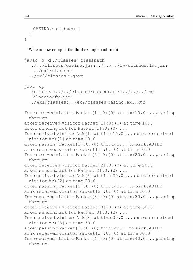
CASINO.shutdown();
}
}
We can now compile the third example and run it:
javac g d ./classes classpath
../../classes/casino.jar:../../../fw/classes/fw.jar:
../ex1/classes:
../ex2/classes *.java
java cp
./classes:../../classes/casino.jar:../../../fw/
classes/fw.jar:
../ex1/classes:../ex2/classes casino.ex3.Run
fsm received visitor Packet[1]:0:(0) at time 10.0 ... passing
through
acker received visitor Packet[1]:0:(0) at time 10.0
acker sending ack for Packet[1]:0:(0) ...
fsm received visitor Ack[1] at time 10.0 ... source received
visitor Ack[1] at time 10.0
acker passing Packet[1]:0:(0) through... to sink.ASIDE
sink received visitor Packet[1]:0:(0) at time 10.0
fsm received visitor Packet[2]:0:(0) at time 20.0 ... passing
through
acker received visitor Packet[2]:0:(0) at time 20.0
acker sending ack for Packet[2]:0:(0) ...
fsm received visitor Ack[2] at time 20.0 ... source received
visitor Ack[2] at time 20.0
acker passing Packet[2]:0:(0) through... to sink.ASIDE
sink received visitor Packet[2]:0:(0) at time 20.0
fsm received visitor Packet[3]:0:(0) at time 30.0 ... passing
through
acker received visitor Packet[3]:0:(0) at time 30.0
acker sending ack for Packet[3]:0:(0) ...
fsm received visitor Ack[3] at time 30.0 ... source received
visitor Ack[3] at time 30.0
acker passing Packet[3]:0:(0) through... to sink.ASIDE
sink received visitor Packet[3]:0:(0) at time 30.0
fsm received visitor Packet[4]:0:(0) at time 40.0 ... passing
through
141 Tutorial 3: Making Visitors
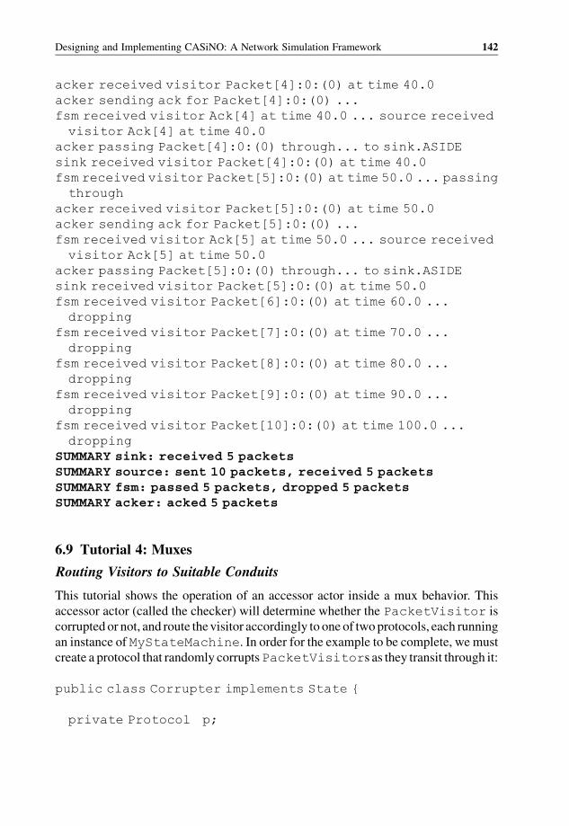
acker received visitor Packet[4]:0:(0) at time 40.0
acker sending ack for Packet[4]:0:(0) ...
fsm received visitor Ack[4] at time 40.0 ... source received
visitor Ack[4] at time 40.0
acker passing Packet[4]:0:(0) through... to sink.ASIDE
sink received visitor Packet[4]:0:(0) at time 40.0
fsm received visitor Packet[5]:0:(0) at time 50.0 ... passing
through
acker received visitor Packet[5]:0:(0) at time 50.0
acker sending ack for Packet[5]:0:(0) ...
fsm received visitor Ack[5] at time 50.0 ... source received
visitor Ack[5] at time 50.0
acker passing Packet[5]:0:(0) through... to sink.ASIDE
sink received visitor Packet[5]:0:(0) at time 50.0
fsm received visitor Packet[6]:0:(0) at time 60.0 ...
dropping
fsm received visitor Packet[7]:0:(0) at time 70.0 ...
dropping
fsm received visitor Packet[8]:0:(0) at time 80.0 ...
dropping
fsm received visitor Packet[9]:0:(0) at time 90.0 ...
dropping
fsm received visitor Packet[10]:0:(0) at time 100.0 ...
dropping
SUMMARY sink: received 5 packetsSUMMARY source: sent 10 packets, received 5 packetsSUMMARY fsm: passed 5 packets, dropped 5 packetsSUMMARY acker: acked 5 packets
6.9 Tutorial 4: Muxes
Routing Visitors to Suitable Conduits
This tutorial shows the operation of an accessor actor inside a mux behavior. This
accessor actor (called the checker) will determine whether the PacketVisitor is
corrupted or not, and route thevisitor accordingly to one of twoprotocols, each running
an instance of MyStateMachine. In order for the example to be complete, we must
create a protocol that randomly corruptsPacketVisitors as they transit through it:
public class Corrupter implements State {
private Protocol p;
Designing and Implementing CASiNO: A Network Simulation Framework 142

public Corrupter() {
}
public void shutdown() {
System.out.println("SUMMARY"+getName()+":corrupted"+
corrupt+" packets");
}
public String getName() {
if ( p!=null) return p.getName();
else return "Corrupter (unnamed)";
}
public void setProtocol(Protocol p) {
p = p;
}
int corrupt = 0;
public boolean handle(Visitor v, Conduit.Side e) {
System.out.println("Corrupter received visitor "+
v+" at time "+Scheduler.getTime());
if (v instanceof PacketVisitor) {
PacketVisitor pv = (PacketVisitor)v;
pv.corrupt();
if (pv.isCorrupt()) {
corrupt++;
}
}
return true;
}
}
Now given that the corrupter will lie between the source and the checker mux, we
know that packets arriving at the checker may ormay not be corrupted.Whenwewrite
the checker, wewill have it keep two references to conduits: the conduit towhich good
(uncorrupt) packets are to be sent; and the conduit towhich bad (corrupt) packets are to
be sent. Below is the Checker class:
public class Checker implements Accessor {
private Mux m;
public Checker() { }
143 Tutorial 4: Muxes
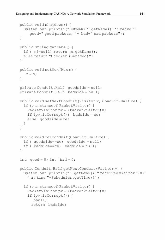
public void shutdown() {
System.out.println("SUMMARY "+getName()+": recvd "+
good+" good packets, "+ bad+" bad packets");
}
public String getName() {
if ( m!=null) return m.getName();
else return "Checker (unnamed)";
}
public void setMux(Mux m) {
m = m;
}
private Conduit.Half goodside = null;
private Conduit.Half badside = null;
public void setNextConduit(Visitor v, Conduit.Half ce) {
if (v instanceof PacketVisitor) {
PacketVisitor pv = (PacketVisitor)v;
if (pv.isCorrupt()) badside = ce;
else goodside = ce;
}
}
public void delConduit(Conduit.Half ce) {
if ( goodside==ce) goodside = null;
if ( badside==ce) badside = null;
}
int good = 0; int bad = 0;
public Conduit.Half getNextConduit(Visitor v) {
System.out.println(""+getName()+"receivedvisitor"+v+
" at time "+Scheduler.getTime());
if (v instanceof PacketVisitor) {
PacketVisitor pv = (PacketVisitor)v;
if (pv.isCorrupt()) {
bad++;
return badside;
Designing and Implementing CASiNO: A Network Simulation Framework 144
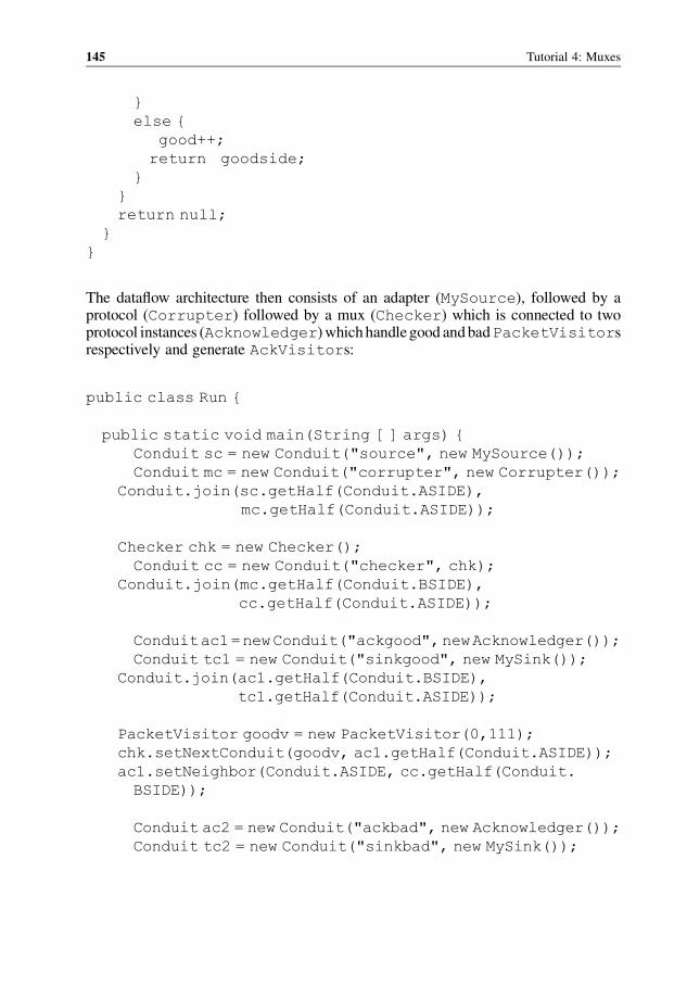
}
else {
good++;
return goodside;
}
}
return null;
}
}
The dataflow architecture then consists of an adapter (MySource), followed by aprotocol (Corrupter) followed by a mux (Checker) which is connected to twoprotocol instances (Acknowledger)whichhandlegood andbadPacketVisitorsrespectively and generate AckVisitors:
public class Run {
public static void main(String [ ] args) {
Conduit sc = new Conduit("source", new MySource());
Conduit mc = new Conduit("corrupter", new Corrupter());
Conduit.join(sc.getHalf(Conduit.ASIDE),
mc.getHalf(Conduit.ASIDE));
Checker chk = new Checker();
Conduit cc = new Conduit("checker", chk);
Conduit.join(mc.getHalf(Conduit.BSIDE),
cc.getHalf(Conduit.ASIDE));
Conduitac1=newConduit("ackgood",newAcknowledger());
Conduit tc1 = new Conduit("sinkgood", new MySink());
Conduit.join(ac1.getHalf(Conduit.BSIDE),
tc1.getHalf(Conduit.ASIDE));
PacketVisitor goodv = new PacketVisitor(0,111);
chk.setNextConduit(goodv, ac1.getHalf(Conduit.ASIDE));
ac1.setNeighbor(Conduit.ASIDE, cc.getHalf(Conduit.
BSIDE));
Conduit ac2 = new Conduit("ackbad", new Acknowledger());
Conduit tc2 = new Conduit("sinkbad", new MySink());
145 Tutorial 4: Muxes

Conduit.join(ac2.getHalf(Conduit.BSIDE),
tc2.getHalf(Conduit.ASIDE));
ac2.setNeighbor(Conduit.ASIDE, cc.getHalf(Conduit.
BSIDE));
PacketVisitor badv = new PacketVisitor(0,222);
while (!badv.isCorrupt()) badv.corrupt();
chk.setNextConduit(badv, ac2.getHalf(Conduit.ASIDE));
Thread t = new Thread(Scheduler.instance());
t.start();
try { t.join(); }
catch (Exception e) { }
CASINO.shutdown();
}
We can now compile the fourth example and run it:
javac g d ./classes classpath ../../classes/casino.
jar:../../../fw/classes/fw.jar:../ex1/classes:../ex2/
classes:../ex3/classes *.java
java cp ./classes:../../classes/casino.jar:../../../fw/
classes/fw.jar:../ex1/classes:../ex2/classes:../ex3/
classes casino.ex4.Run
Corrupter received visitor Packet[1]:0:(0) at time 10.0
checker received visitor Packet[1]:0:(0) at time 10.0
ackgood received visitor Packet[1]:0:(0) at time 10.0
ackgood sending ack for Packet[1]:0:(0) ...
Corrupter received visitor Ack[1] at time 10.0
source received visitor Ack[1] at time 10.0
ackgood passing Packet[1]:0:(0) through... to sinkgood.
ASIDE
sinkgood received visitor Packet[1]:0:(0) at time 10.0
Corrupter received visitor Packet[2]:0:(0) at time 20.0
checker received visitor Packet[2]:0:(0) at time 20.0
ackgood received visitor Packet[2]:0:(0) at time 20.0
ackgood sending ack for Packet[2]:0:(0) ...
Corrupter received visitor Ack[2] at time 20.0
source received visitor Ack[2] at time 20.0
Designing and Implementing CASiNO: A Network Simulation Framework 146
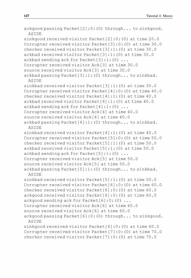
ackgood passing Packet[2]:0:(0) through... to sinkgood.
ASIDE
sinkgood received visitor Packet[2]:0:(0) at time 20.0
Corrupter received visitor Packet[3]:0:(0) at time 30.0
checker received visitor Packet[3]:1:(0) at time 30.0
ackbad received visitor Packet[3]:1:(0) at time 30.0
ackbad sending ack for Packet[3]:1:(0) ...
Corrupter received visitor Ack[3] at time 30.0
source received visitor Ack[3] at time 30.0
ackbad passing Packet[3]:1:(0) through... to sinkbad.
ASIDE
sinkbad received visitor Packet[3]:1:(0) at time 30.0
Corrupter received visitor Packet[4]:0:(0) at time 40.0
checker received visitor Packet[4]:1:(0) at time 40.0
ackbad received visitor Packet[4]:1:(0) at time 40.0
ackbad sending ack for Packet[4]:1:(0) ...
Corrupter received visitor Ack[4] at time 40.0
source received visitor Ack[4] at time 40.0
ackbad passing Packet[4]:1:(0) through... to sinkbad.
ASIDE
sinkbad received visitor Packet[4]:1:(0) at time 40.0
Corrupter received visitor Packet[5]:0:(0) at time 50.0
checker received visitor Packet[5]:1:(0) at time 50.0
ackbad received visitor Packet[5]:1:(0) at time 50.0
ackbad sending ack for Packet[5]:1:(0) ...
Corrupter received visitor Ack[5] at time 50.0
source received visitor Ack[5] at time 50.0
ackbad passing Packet[5]:1:(0) through... to sinkbad.
ASIDE
sinkbad received visitor Packet[5]:1:(0) at time 50.0
Corrupter received visitor Packet[6]:0:(0) at time 60.0
checker received visitor Packet[6]:0:(0) at time 60.0
ackgood received visitor Packet[6]:0:(0) at time 60.0
ackgood sending ack for Packet[6]:0:(0) ...
Corrupter received visitor Ack[6] at time 60.0
source received visitor Ack[6] at time 60.0
ackgood passing Packet[6]:0:(0) through... to sinkgood.
ASIDE
sinkgood received visitor Packet[6]:0:(0) at time 60.0
Corrupter received visitor Packet[7]:0:(0) at time 70.0
checker received visitor Packet[7]:0:(0) at time 70.0
147 Tutorial 4: Muxes
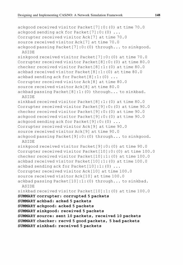
ackgood received visitor Packet[7]:0:(0) at time 70.0
ackgood sending ack for Packet[7]:0:(0) ...
Corrupter received visitor Ack[7] at time 70.0
source received visitor Ack[7] at time 70.0
ackgood passing Packet[7]:0:(0) through... to sinkgood.
ASIDE
sinkgood received visitor Packet[7]:0:(0) at time 70.0
Corrupter received visitor Packet[8]:0:(0) at time 80.0
checker received visitor Packet[8]:1:(0) at time 80.0
ackbad received visitor Packet[8]:1:(0) at time 80.0
ackbad sending ack for Packet[8]:1:(0) ...
Corrupter received visitor Ack[8] at time 80.0
source received visitor Ack[8] at time 80.0
ackbad passing Packet[8]:1:(0) through... to sinkbad.
ASIDE
sinkbad received visitor Packet[8]:1:(0) at time 80.0
Corrupter received visitor Packet[9]:0:(0) at time 90.0
checker received visitor Packet[9]:0:(0) at time 90.0
ackgood received visitor Packet[9]:0:(0) at time 90.0
ackgood sending ack for Packet[9]:0:(0) ...
Corrupter received visitor Ack[9] at time 90.0
source received visitor Ack[9] at time 90.0
ackgood passing Packet[9]:0:(0) through... to sinkgood.
ASIDE
sinkgood received visitor Packet[9]:0:(0) at time 90.0
Corrupter received visitor Packet[10]:0:(0) at time 100.0
checker received visitor Packet[10]:1:(0) at time 100.0
ackbad received visitor Packet[10]:1:(0) at time 100.0
ackbad sending ack for Packet[10]:1:(0) ...
Corrupter received visitor Ack[10] at time 100.0
source received visitor Ack[10] at time 100.0
ackbad passing Packet[10]:1:(0) through... to sinkbad.
ASIDE
sinkbad received visitor Packet[10]:1:(0) at time 100.0
SUMMARY corrupter: corrupted 5 packetsSUMMARY ackbad: acked 5 packetsSUMMARY ackgood: acked 5 packetsSUMMARY sinkgood: received 5 packetsSUMMARY source: sent 10 packets, received 10 packetsSUMMARY checker: recvd 5 good packets, 5 bad packetsSUMMARY sinkbad: received 5 packets
Designing and Implementing CASiNO: A Network Simulation Framework 148
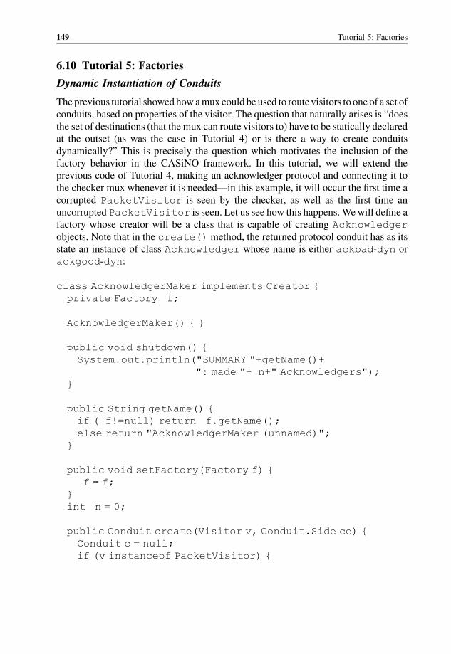
6.10 Tutorial 5: Factories
Dynamic Instantiation of Conduits
The previous tutorial showedhowamux could be used to routevisitors to one of a set of
conduits, based on properties of the visitor. The question that naturally arises is “does
the set of destinations (that the mux can route visitors to) have to be statically declared
at the outset (as was the case in Tutorial 4) or is there a way to create conduits
dynamically?” This is precisely the question which motivates the inclusion of the
factory behavior in the CASiNO framework. In this tutorial, we will extend the
previous code of Tutorial 4, making an acknowledger protocol and connecting it to
the checker mux whenever it is needed—in this example, it will occur the first time a
corrupted PacketVisitor is seen by the checker, as well as the first time an
uncorrupted PacketVisitor is seen. Let us see how this happens.Wewill define a
factory whose creator will be a class that is capable of creating Acknowledger
objects. Note that in the create() method, the returned protocol conduit has as its
state an instance of class Acknowledger whose name is either ackbad-dyn or
ackgood-dyn:
class AcknowledgerMaker implements Creator {
private Factory f;
AcknowledgerMaker() { }
public void shutdown() {
System.out.println("SUMMARY "+getName()+
": made "+ n+" Acknowledgers");
}
public String getName() {
if ( f!=null) return f.getName();
else return "AcknowledgerMaker (unnamed)";
}
public void setFactory(Factory f) {
f = f;
}
int n = 0;
public Conduit create(Visitor v, Conduit.Side ce) {
Conduit c = null;
if (v instanceof PacketVisitor) {
149 Tutorial 5: Factories
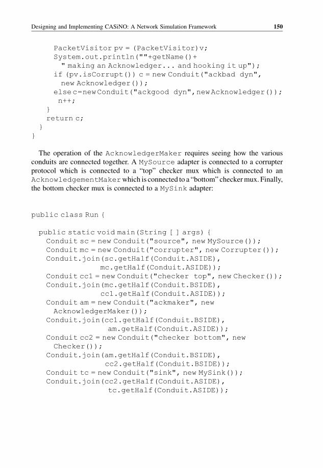
PacketVisitor pv = (PacketVisitor)v;
System.out.println(""+getName()+
" making an Acknowledger... and hooking it up");
if (pv.isCorrupt()) c = new Conduit("ackbad dyn",
new Acknowledger());
elsec=newConduit("ackgood dyn",newAcknowledger());
n++;
}
return c;
}
}
The operation of the AcknowledgerMaker requires seeing how the various
conduits are connected together. A MySource adapter is connected to a corrupter
protocol which is connected to a “top” checker mux which is connected to an
AcknowledgementMakerwhich is connected to a “bottom” checkermux. Finally,
the bottom checker mux is connected to a MySink adapter:
public class Run {
public static void main(String [ ] args) {
Conduit sc = new Conduit("source", new MySource());
Conduit mc = new Conduit("corrupter", new Corrupter());
Conduit.join(sc.getHalf(Conduit.ASIDE),
mc.getHalf(Conduit.ASIDE));
Conduit cc1 = new Conduit("checker top", new Checker());
Conduit.join(mc.getHalf(Conduit.BSIDE),
cc1.getHalf(Conduit.ASIDE));
Conduit am = new Conduit("ackmaker", new
AcknowledgerMaker());
Conduit.join(cc1.getHalf(Conduit.BSIDE),
am.getHalf(Conduit.ASIDE));
Conduit cc2 = new Conduit("checker bottom", new
Checker());
Conduit.join(am.getHalf(Conduit.BSIDE),
cc2.getHalf(Conduit.BSIDE));
Conduit tc = new Conduit("sink", new MySink());
Conduit.join(cc2.getHalf(Conduit.ASIDE),
tc.getHalf(Conduit.ASIDE));
Designing and Implementing CASiNO: A Network Simulation Framework 150
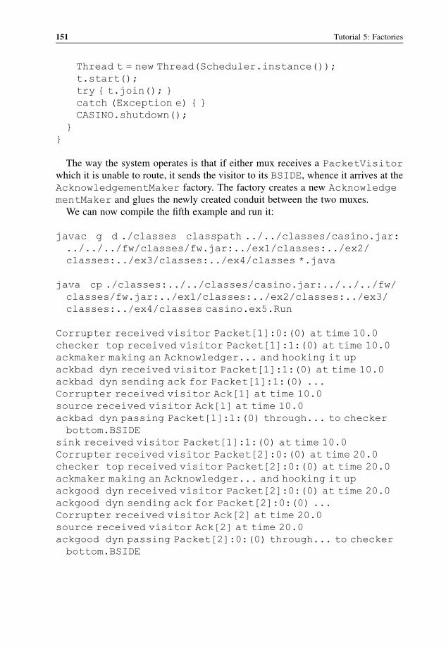
Thread t = new Thread(Scheduler.instance());
t.start();
try { t.join(); }
catch (Exception e) { }
CASINO.shutdown();
}
}
The way the system operates is that if either mux receives a PacketVisitor
which it is unable to route, it sends the visitor to its BSIDE, whence it arrives at the
AcknowledgementMaker factory. The factory creates a new Acknowledge
mentMaker and glues the newly created conduit between the two muxes.
We can now compile the fifth example and run it:
javac g d ./classes classpath ../../classes/casino.jar:
../../../fw/classes/fw.jar:../ex1/classes:../ex2/
classes:../ex3/classes:../ex4/classes *.java
java cp ./classes:../../classes/casino.jar:../../../fw/
classes/fw.jar:../ex1/classes:../ex2/classes:../ex3/
classes:../ex4/classes casino.ex5.Run
Corrupter received visitor Packet[1]:0:(0) at time 10.0
checker top received visitor Packet[1]:1:(0) at time 10.0
ackmaker making an Acknowledger... and hooking it up
ackbad dyn received visitor Packet[1]:1:(0) at time 10.0
ackbad dyn sending ack for Packet[1]:1:(0) ...
Corrupter received visitor Ack[1] at time 10.0
source received visitor Ack[1] at time 10.0
ackbad dyn passing Packet[1]:1:(0) through... to checker
bottom.BSIDE
sink received visitor Packet[1]:1:(0) at time 10.0
Corrupter received visitor Packet[2]:0:(0) at time 20.0
checker top received visitor Packet[2]:0:(0) at time 20.0
ackmaker making an Acknowledger... and hooking it up
ackgood dyn received visitor Packet[2]:0:(0) at time 20.0
ackgood dyn sending ack for Packet[2]:0:(0) ...
Corrupter received visitor Ack[2] at time 20.0
source received visitor Ack[2] at time 20.0
ackgood dyn passing Packet[2]:0:(0) through... to checker
bottom.BSIDE
151 Tutorial 5: Factories
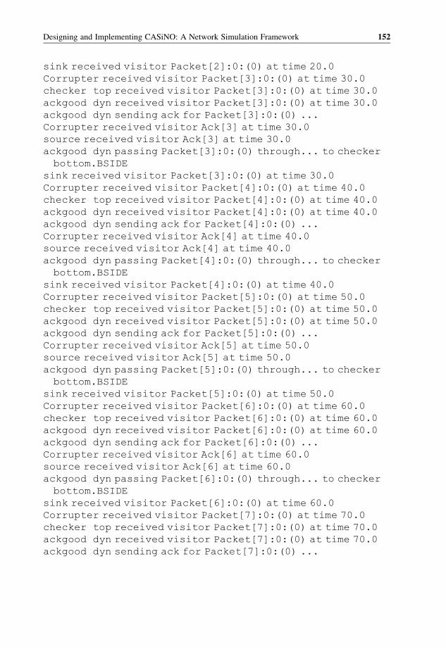
sink received visitor Packet[2]:0:(0) at time 20.0
Corrupter received visitor Packet[3]:0:(0) at time 30.0
checker top received visitor Packet[3]:0:(0) at time 30.0
ackgood dyn received visitor Packet[3]:0:(0) at time 30.0
ackgood dyn sending ack for Packet[3]:0:(0) ...
Corrupter received visitor Ack[3] at time 30.0
source received visitor Ack[3] at time 30.0
ackgood dyn passing Packet[3]:0:(0) through... to checker
bottom.BSIDE
sink received visitor Packet[3]:0:(0) at time 30.0
Corrupter received visitor Packet[4]:0:(0) at time 40.0
checker top received visitor Packet[4]:0:(0) at time 40.0
ackgood dyn received visitor Packet[4]:0:(0) at time 40.0
ackgood dyn sending ack for Packet[4]:0:(0) ...
Corrupter received visitor Ack[4] at time 40.0
source received visitor Ack[4] at time 40.0
ackgood dyn passing Packet[4]:0:(0) through... to checker
bottom.BSIDE
sink received visitor Packet[4]:0:(0) at time 40.0
Corrupter received visitor Packet[5]:0:(0) at time 50.0
checker top received visitor Packet[5]:0:(0) at time 50.0
ackgood dyn received visitor Packet[5]:0:(0) at time 50.0
ackgood dyn sending ack for Packet[5]:0:(0) ...
Corrupter received visitor Ack[5] at time 50.0
source received visitor Ack[5] at time 50.0
ackgood dyn passing Packet[5]:0:(0) through... to checker
bottom.BSIDE
sink received visitor Packet[5]:0:(0) at time 50.0
Corrupter received visitor Packet[6]:0:(0) at time 60.0
checker top received visitor Packet[6]:0:(0) at time 60.0
ackgood dyn received visitor Packet[6]:0:(0) at time 60.0
ackgood dyn sending ack for Packet[6]:0:(0) ...
Corrupter received visitor Ack[6] at time 60.0
source received visitor Ack[6] at time 60.0
ackgood dyn passing Packet[6]:0:(0) through... to checker
bottom.BSIDE
sink received visitor Packet[6]:0:(0) at time 60.0
Corrupter received visitor Packet[7]:0:(0) at time 70.0
checker top received visitor Packet[7]:0:(0) at time 70.0
ackgood dyn received visitor Packet[7]:0:(0) at time 70.0
ackgood dyn sending ack for Packet[7]:0:(0) ...
Designing and Implementing CASiNO: A Network Simulation Framework 152
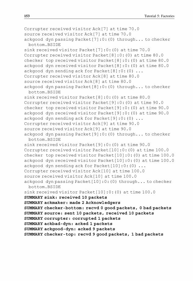
Corrupter received visitor Ack[7] at time 70.0
source received visitor Ack[7] at time 70.0
ackgood dyn passing Packet[7]:0:(0) through... to checker
bottom.BSIDE
sink received visitor Packet[7]:0:(0) at time 70.0
Corrupter received visitor Packet[8]:0:(0) at time 80.0
checker top received visitor Packet[8]:0:(0) at time 80.0
ackgood dyn received visitor Packet[8]:0:(0) at time 80.0
ackgood dyn sending ack for Packet[8]:0:(0) ...
Corrupter received visitor Ack[8] at time 80.0
source received visitor Ack[8] at time 80.0
ackgood dyn passing Packet[8]:0:(0) through... to checker
bottom.BSIDE
sink received visitor Packet[8]:0:(0) at time 80.0
Corrupter received visitor Packet[9]:0:(0) at time 90.0
checker top received visitor Packet[9]:0:(0) at time 90.0
ackgood dyn received visitor Packet[9]:0:(0) at time 90.0
ackgood dyn sending ack for Packet[9]:0:(0) ...
Corrupter received visitor Ack[9] at time 90.0
source received visitor Ack[9] at time 90.0
ackgood dyn passing Packet[9]:0:(0) through... to checker
bottom.BSIDE
sink received visitor Packet[9]:0:(0) at time 90.0
Corrupter received visitor Packet[10]:0:(0) at time 100.0
checker top received visitor Packet[10]:0:(0) at time 100.0
ackgood dyn received visitor Packet[10]:0:(0) at time 100.0
ackgood dyn sending ack for Packet[10]:0:(0) ...
Corrupter received visitor Ack[10] at time 100.0
source received visitor Ack[10] at time 100.0
ackgood dyn passing Packet[10]:0:(0) through... to checker
bottom.BSIDE
sink received visitor Packet[10]:0:(0) at time 100.0
SUMMARY sink: received 10 packetsSUMMARY ackmaker: made 2 AcknowledgersSUMMARY checker-bottom: recvd 0 good packets, 0 bad packetsSUMMARY source: sent 10 packets, received 10 packetsSUMMARY corrupter: corrupted 1 packetsSUMMARY ackbad-dyn: acked 1 packetsSUMMARY ackgood-dyn: acked 9 packetsSUMMARY checker-top: recvd 9 good packets, 1 bad packets
153 Tutorial 5: Factories
6.11 Summary
In this chapter, we developed an extension to the discrete-event simulation framework
of Chapter 2. This framework, called the Component Architecture for Simulating
Network Objects (CASiNO), is based on parallel hierarchies of behaviors and actors,
codifying the principal functional classes of components within a network protocol
simulation. CASiNO provides us with many desirable features:
1. Ease of design: Implementations of protocols “from the ground up” (e.g., in a
programming language like Java) require substantial effort to implement
common communication constructs, such as timers, message queues, etc.
Given a general-purpose language like Java, a programmer can build these
in many different ways. A framework, on the other hand, assumes responsi-
bility for all the common low-level aspects of the protocol’s implementation,
while providing high-level abstractions with which a programmer can quickly
specify the logical structure of the protocol. A framework’s power comes from
the way in which it reduces the number of ways in which the programmer can
implement a protocol. The key is to carry out this reduction without sacrificing
the range of what the programmer can accomplish. Implementations that use a
framework are more “uniform” in their design because the number of arbitrary
choices is reduced, causing programs to conform to the common structure
imposed on them. This structure makes the design and maintenance process
simpler.
2. Ease of description: By providing common high-level abstractions with which
protocols can be quickly implemented, a framework also implicitly provides a
succinct language by which to describe and document the design of protocol
software.
3. Ease of maintenance: Ease of descriptions makes it easier to maintain modular
communication protocol software.
4. Portability: An ideal framework will hide many system-dependent operations,
exposing only the high-level abstractions needed for protocol development. Porting
a protocol to a new platform amounts to porting the framework itself to the new
platform. This process only needs to be carried out once; subsequently, any
protocols implemented using the framework will also operate on the new
architecture.
5. Longevity of code: Because implementations over a framework are easy to
describe and easy to port, the learning curve for implementations is also
relatively short, making projects less susceptible to personnel and hardware
changes.
6. Visualization: Because code is written using high-level abstractions, the invoca-
tion of these abstractions can be logged at run time, and subsequently visualized.
Designing and Implementing CASiNO: A Network Simulation Framework 154
Recommended Reading
[1] A. Battou, B. Khan, D. Lee, S. Mountcastle, D. Talmage, and S. Marsh, “CASINO: Component
Architecture for Simulating Network Objects,” Software Practice and Experience, vol. 32,
pp. 1099 1128, 2002.
[2] A. Battou, B. Khan, D. Lee, S. Marsh, S. Mountcastle, and D. Talmage, “CASiNO: A Component
Architecture for Simulation of Network Objects,” Proceedings of the 1999 Symposium on Perfor
mance Evaluation of Computer and Telecommunication Systems, Chicago, Illinois, July 11 15,
Society for Computer Simulation, 1999, pp. 261 272.
[3] E. Gamma, R. Helm, R. Johnson, and J. Vlissides, Design Patterns: Elements of Object Oriented
Software, Addison Wesley, 1995.
[4] L. P. Deutsch, “Design reuse and frameworks in the Smalltalk 80 system,” in Software Reusability,
Volume II: Applications and Experience (T. J. Biggerstaff and A. J. Perlis, eds.), Addison Wesley,
1989.
[5] R. E. Johnson andB. Foote, “Designing reusable classes,” Journal ofObject Oriented Programming,
vol. 1, pp. 22 35, 1988.
[6] S. Mountcastle, D. Talmage, B. Khan, S. Marsh, A. Battou, and D. Lee, “Introducing SEAN: the
signaling entity for ATM networks,” Proceedings of IEEE GLOBECOM’00, San Francisco,
California, IEEE, 2000, pp. 532 537.
[7] A. Battou, B. Khan, S. Marsh, S. Mountcastle, and D. Talmage, “Introducing PRouST: the PNNI
routing and simulation toolkit,” Proceedings of the IEEE Workshop on High Performance
Switching and Routing, Dallas, Texas, IEEE, 2001, pp. 335 341.
[8] G. B. Brahim, B. Khan, A. Battou, M. Guizani, and G. Chaudhry, “TRON: The Toolkit for Routing
in Optical Networks,” in Proceedings of IEEE GLOBECOM’01, San Antonio, Texas, IEEE, 2001,
pp. 1445 1449.
[9] P. Nikander and A. Karila, “A Java Beans component architecture for cryptographic protocols,”
Proceedings of the 7th USENIX Security Symposium, San Antonio, Texas, 1998.
[10] L.Breslau,D.Estrin,K.Fall, S. Floyd, J.Heidemann,A.Helmy, P.Huang, S.McCanne,K.Varadhan,
Y. Xu, and H. Yu, “Advances in network simulation,” IEEE Computer, pp. 59 67, May 2000.
[11] S. Keshav, An Engineering Approach to Computer Networking: ATM Networks, the Internet, and
the Telephone Network, Addison Wesley, 1997.
[12] A. S. Tanenbaum, Computer Networks, 3rd Edition, Prentice Hall PTR, 1996.
[13] D. E. Comer, Internetworking with TCP/IP, 3rd Edition, Volume 1, Prentice Hall, 1995.
[14] Online: http://www.isi.edu/nsnam/ns/
155 Recommended Reading


7
Statistical Distributions andRandom Number Generation
Generally,modeling and simulation are developed due to the interest in studying and
predicting the behaviors of real systems (and hence verifying the correctness of
abstract models). Theoretical analysis of models of systems is typically validated by
simulation results, which are considered as an empirical proof of the model’s
correctness. Simulations thus offer a framework for the study of systems and
models.
Simulation engineers use simulators to study the behaviors and correctness of
systems by observing the output information generated by a simulator given its input
specifications. In such cases, a crucial task in developing simulations is to determine
the complete input to the simulator. In order to achieve this, one often must make
random choices. For example, in a communication system, node A and node B
communicate exactly once every T seconds, where T is determined by choosing a
random number in the range of [0, 10]. This is an example of a statistical distribution,
which is a formal means of specifying the relative likelihood of different system
inputs.
In the rest of this chapter, a set of statistical distributions that could be used in
simulation as well as a set of random number generation techniques are discussed.We
provide an overview of statistical distributions as well as discrete distributions. Then,
continuous distributions and descriptions of some known ones are discussed in detail.
Then, an overview of the concepts and issues surrounding the generation of random
numbers is presented. A random number generator (RNG) is a process that emits a
sequence of numbers that permit the construction of a segment of a sample path of the
random process being modeled.
Network Modeling and Simulation M. Guizani, A. Rayes, B. Khan and A. Al Fuqaha
� 2010 John Wiley & Sons, Ltd.
7.1 Introduction to Statistical Distributions
A continuous random variable is a variable that takes random values over a continuous
set of possibilities. A discrete random variable is a variable that takes random values
over a finite (or countably infinite) set of possibilities. The height of a randomly
selected human being is an example of a continuous random variable. The year of birth
of a randomly selected human being is an example of a discrete random variable.
7.1.1 Probability Density Functions
LetX be a continuous randomvariable on the interval [a,b]. If the probability thatX lies
in the interval [a, b] can be expressed by the following function:
Pða � X � bÞ ¼ðba
f ðxÞdx
then the function f(x) is called probability density function (PDF) of the random
variable. A PDF satisfies the following conditions:
f ðxÞ � 0 for all x in ½a; b�ðba
f ðxÞdx ¼ 1
f ðxÞ ¼ 0 if x is not in ½a; b�:
The function f(x) also has the following properties:
For any specific value x0; PðX ¼ x0Þ ¼ 0 ¼ðx0x0
f ðxÞdx
Pðx � X � bÞ ¼ Pðx < X � bÞ ¼ Pðx � X < bÞ ¼ Pðx < X < bÞ:
Discrete random variables do not have a PDF. However, it is possible to represent
certain discrete random variables using a density of probability, via the Dirac delta
function.
7.1.2 Cumulative Density Functions
The cumulative density function (CDF) measures the probability that a random
variable X assumes a value less than or equal to a specific value. By convention, if
the PDF is denoted by f(x), then the CDF is denoted by F(x). Unlike the PDF, the CDF
is able to quantify both discrete and continues random variables.
Statistical Distributions and Random Number Generation 158

The CDF for a discrete random variable X is:
FðxÞ ¼X
all xi�x
pðxiÞ:
The CDF for a continuous random variable is:
FðxÞ ¼ðx1f ðtÞdt:
Moreover, the probability of a random variable in a range can be expressed as
follows:
Pða < X � bÞ ¼ FðaÞ FðbÞ for all a < b:
The function F(x) has the following properties:
(a) F is an increasing function such that; if a < b; then FðaÞ � FðbÞ(b) limx! þ1 FðxÞ ¼ 1
(c) limx! 1 FðxÞ ¼ 0:
7.1.3 Joint and Marginal Distributions
Suppose that there are two random variables X and Y, which might have the same or
different probability distributions. IfX and Y are random variables, then (X, Y) is also
a random variable taking values in the Cartesian product of the spaces fromwhich X
and Y are drawn. The distribution of the random variable (X, Y) is called the joint
distribution ofX and Y, and is denoted by (X, Y). The distributions ofX and Y are each
referred to asmarginal distributions. For example, suppose we have two fair dice, a
red one and a green one. The roll of the red die is the variable X1, while the variable
X2 is used to represent the value of the roll of the green die. We record the output X1,
X2 after each roll of the pair, and define X¼X1 þ X2 and Y¼X1 X2. The
probability distribution of (X, Y) is called a joint distribution and the probability
distribution of X and Y is called a marginal distribution.
7.1.4 Correlation and Covariance
The covariance of random variables X and Y measures the relation between X and Y.
Intuitively, when X and Y are independent of one another, the covariance gives a score
159 Introduction to Statistical Distributions

around 0. But if the variables are dependent, their covariance is high. The covariance is
computed as:
covðX; YÞ ¼ E½ðX mxÞðY myÞ�such that mx is the mean of X and my is the mean of Y:
The correlation measures the strength of the linear dependence between X and Y.
The values of the correlation function are in the range of 1 and 1. The formula to
calculate the correlation is:
rx;y ¼covðX; YÞvarðXÞvarðYÞp where var is the variance function:
7.1.5 Discrete versus Continuous Distributions
Continuous distributions describe the distribution of continuous random variables. A
probability distribution is continuous if its CDF is continuous. For example, we can
consider the probability distribution of the time we spend waiting for the bus each
morning. If the bus arrives every 20minutes starting at 6.00 a.m. (until 8.00 a.m.) and if
we arrive at the bus stop at a random time in this 2 hour interval, then the probability that
wewait a period of time t has a continuous distribution (since t is a continuous variable).
Discrete distributions describe continuous distributions which are zero on all but a
finite (or countably infinite) set of values. A probability distribution is discrete if its
CDF increases in quantized steps. The Bernoulli and binomial distributions are
examples of a discrete distribution. As an example of a discrete distribution, consider
a game of chance in which we pick numbers from the set {1, 2, 3, 4, 5}. The number of
possible values in this case is finite. Therefore, the game gives rise to a discrete random
variable (the value of the number selected) and the distribution of this random variable
is a discrete distribution.
7.2 Discrete Distributions
Discrete distributions describe the statistical distribution of discrete random variables.
In the following, we discuss four discrete distributions which are the Bernoulli
distribution, the binomial distribution, the geometric distribution, and the Poisson
distribution.
7.2.1 Bernoulli Distribution
Consider an experiment consisting of n independent trials. The result of each trial j
is success or value 1 with probability p or value 0 for a fail with probability q¼ 1 p.
Statistical Distributions and Random Number Generation 160

So, if X is a random variable from a Bernoulli distribution, we have PðX ¼ 1Þ ¼1 PðX ¼ 0Þ ¼ 1 q ¼ p.
The equation of the Bernoulli distribution (its probability mass function) is:
pðX ¼ xjÞ ¼p xj ¼ 1; j ¼ 1; 2; 3; . . . ; n
1 p ¼ q xj ¼ 0; j ¼ 1; 2; 3; . . . ; n
0 otherwise:
8><>:
The mean and variance of Xj are calculated as follows:
EðXjÞ ¼ 0:qþ 1:p ¼ p
VðXjÞ ¼ pð1 pÞ:As an example of the Bernoulli distribution, we can consider the famous coin-
flipping game. This game consists of flipping a (biased) coinmany times and each time
considering whether we get heads or tails. Sampling a random variable that is known
(or assumed) to have a Bernoulli distribution is easy using Java. The following code
achieves this, returning true with probability p and false with probability 1 p. The
code is built using the Java Math.random() function, which chooses random
numbers on the unit interval uniformly at random (justification of the correctness of
this code will be clarified in Section 7.7):
public static boolean bernoulli(double p) {
return Math.random() < p;
}
7.2.2 Binomial Distribution
The binomial distribution is a discrete distribution defined by the number of successes
in a sequence of n binomial trials. The random variable X that denotes the number of
successes in nBernoulli trials follows the Binomial distribution, where the probability
is provided by the following formula:
pðX ¼ xÞ ¼n
x
!pxð1 pÞn x
x ¼ 0; 1; 2; . . . ; n
0 otherwise
8><>:
such thatn
x
!¼ n!
x!ðn xÞ! :
161 Discrete Distributions
The mean and variance of X are calculated as follows:
EðXÞ ¼ np
VðXÞ ¼ npq:
As an example of the binomial distribution, consider the example of our coin-
flipping game. Using the binomial distribution, we can calculate the probability of
having exactly x successes in the game. In practice, when sampling a random variable
that is known (or assumed) to have a binomial distribution, a normal distribution is
approximated. This will be discussed in more detail in Section 7.3.2.
7.2.3 Geometric Distribution
The geometric distribution is a discrete distribution defined by the probability of
getting a “run” of consecutive successes in a Bernoulli experiment, followed by a
failure (e.g., a sequence of n heads, followed by a tail). The probability of a random
variable X that has a geometric distribution is:
pðX ¼ kÞ ¼ pk 1ð1 pÞ:This is based on a Bernoulli experiment that has p as the probability of success (and
1 p as the probability of failure). Themean and variance ofX are calculated as follows:
EðXÞ ¼ 1
p
VðXÞ ¼ 1 p
p2:
As an example of the geometric distribution, consider our game of flipping a coin.
Using the geometric distribution, we can calculate the probability of getting a run of x
heads followed by a single tail in the game. Again, it is easy to sample a random
variable that is known (or assumed) to have a geometric distribution, using Java. The
following code achieves this, taking as an argument the probability of success in the
underlying Bernoulli experiment and returning an integer, chosen according to the
geometric distribution. The code is built using the Java Math.random() function,
which chooses random numbers on the unit interval uniformly at random (again,
justification of the correctness of this code will become clear in Section 7.7):
public static int geometric(double p) {
return (int) Math.ceil(Math.log(Math.random()) / Math.
log(1.0 p));
}
Statistical Distributions and Random Number Generation 162
7.2.4 Poisson Distribution
The PDF of the Poisson distribution is given by the following formula:
pðX ¼ xÞ ¼e 1ax
x!x ¼ 0; 1; . . .
0 otherwise:
8<:
The CDF of the function is
Fð0 < X � xÞ ¼Xxi 0
e aai
i!:
The mean and variance of X are follows:
EðXÞ ¼ a
VðXÞ ¼ a:
As an example of the Poisson distribution, consider a maintenance person who is
beeped each time there is a service call. The number of beeps per hour is a random
variable, taken to have a Poisson distribution with mean a. In order to calculate theprobability that the maintenance person receives no more than m beeps in an hour,
the CDF of the Poisson distribution stated above is used. Again, Java can be used to
sample a random variable that is known (or assumed) to have a Poisson distribution.
The following code achieves this, taking as an argument the intensity a and
returning an integer, chosen according to the Poisson distribution of the specified
intensity. The code is built using the Java Math.random() function, which
chooses random numbers on the unit interval uniformly at random (justification of
the correctness of this code will become clear in Section 7.7 when we discuss
random variate generation):
public static int poisson(double lambda) {
int k = 0;
double p = 1.0;
double L = Math.exp( lambda);
do {
k++;
p *= Math.random();
} while (p >= L);
return k 1;
}
163 Discrete Distributions
7.3 Continuous Distributions
A continuous random variable is a variable that takes random values over a continuous
set of possible values. Continuous random variables can be defined using continuous
PDFs, and in this section we describe some of the most common choices for these
distributions.
7.3.1 Uniform Distribution
A randomvariableX is uniformly distributed on the interval [a, b] if its PDF is given by
the following function:
f ðxÞ ¼1
b aa � x � b
0 otherwise:
8<:
In this case, the CDF is given by:
FðxÞ ¼0 x < a
x a
b aa � x < b
1 x � b:
8>><>>:
The mean and variance of X are calculated as follows:
EðXÞ ¼ aþ b
2
VðXÞ ¼ ðb aÞ212
:
As an example of the uniform distribution, let us consider the random variable X
such thatXmeasures the time period for a passenger waiting at a bus stop to get a bus.
The bus arrives every 20 minutes starting at 6.00 a.m. and ending at 7.00 a.m. The
passenger does not know the schedule but arrives at the bus stop randomly between
6.30 a.m. and 7.00 a.m. The waiting time of the passenger follows a uniform
distribution. Again, Java can be used to sample a random variable that is known
(or assumed) to have a uniform distribution. The following code achieves this, taking
as an argument the interval boundaries a and b, and returning a “double,” chosen
according to the uniform distribution on this interval. The code is built using the Java
Math.random() function, which chooses random numbers on the unit interval
Statistical Distributions and Random Number Generation 164
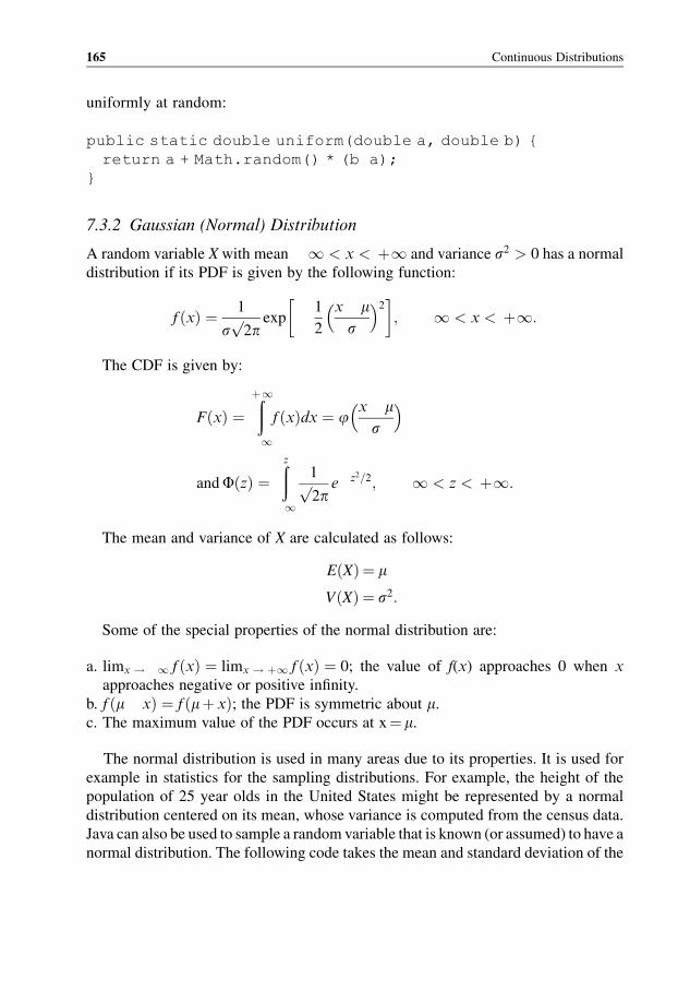
uniformly at random:
public static double uniform(double a, double b) {
return a + Math.random() * (b a);
}
7.3.2 Gaussian (Normal) Distribution
A random variable Xwith mean 1 < x < þ1 and variance s2 > 0 has a normal
distribution if its PDF is given by the following function:
f ðxÞ ¼ 1
s 2pp exp
1
2
x ms
� �2� �; 1 < x < þ1:
The CDF is given by:
FðxÞ ¼ðþ1
1f ðxÞdx ¼ j
x ms
� �
andFðzÞ ¼ðz1
1
2pp e z2=2; 1 < z < þ1:
The mean and variance of X are calculated as follows:
EðXÞ ¼ m
VðXÞ ¼ s2:
Some of the special properties of the normal distribution are:
a. limx ! 1 f ðxÞ ¼ limx ! þ1 f ðxÞ ¼ 0; the value of f(x) approaches 0 when x
approaches negative or positive infinity.
b. f ðm xÞ ¼ f ðmþ xÞ; the PDF is symmetric about m.c. The maximum value of the PDF occurs at x¼ m.
The normal distribution is used in many areas due to its properties. It is used for
example in statistics for the sampling distributions. For example, the height of the
population of 25 year olds in the United States might be represented by a normal
distribution centered on its mean, whose variance is computed from the census data.
Java can also be used to sample a random variable that is known (or assumed) to have a
normal distribution. The following code takes the mean and standard deviation of the
165 Continuous Distributions
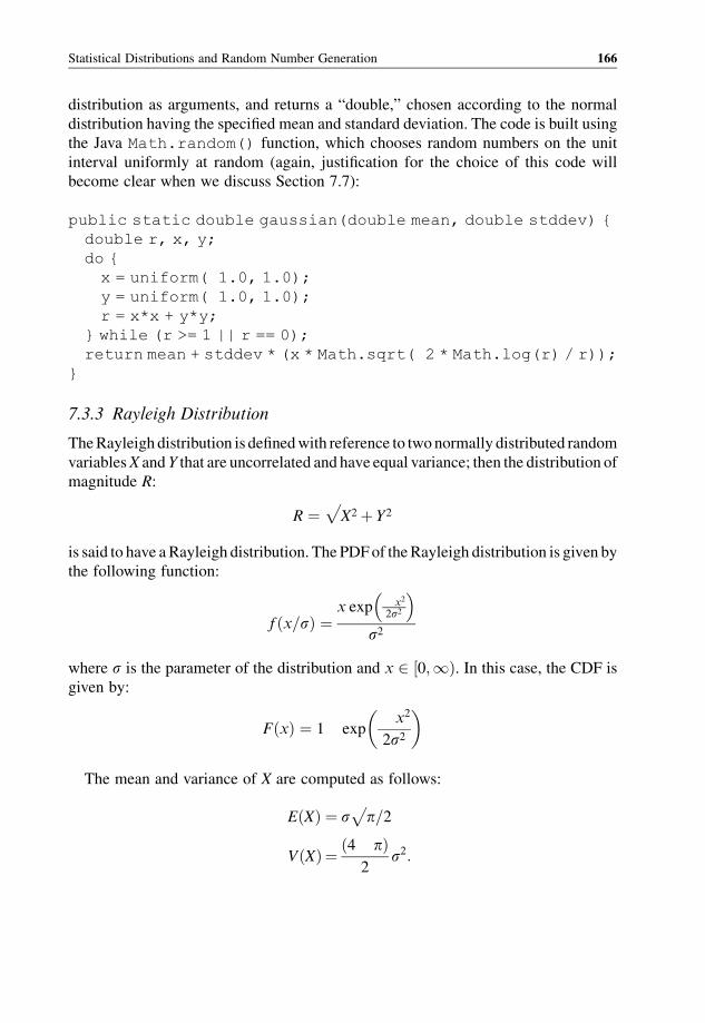
distribution as arguments, and returns a “double,” chosen according to the normal
distribution having the specified mean and standard deviation. The code is built using
the Java Math.random() function, which chooses random numbers on the unit
interval uniformly at random (again, justification for the choice of this code will
become clear when we discuss Section 7.7):
public static double gaussian(double mean, double stddev) {
double r, x, y;
do {
x = uniform( 1.0, 1.0);
y = uniform( 1.0, 1.0);
r = x*x + y*y;
} while (r >= 1 || r == 0);
return mean + stddev * (x * Math.sqrt( 2 * Math.log(r) / r));
}
7.3.3 Rayleigh Distribution
TheRayleigh distribution is definedwith reference to twonormally distributed random
variablesX andY that are uncorrelated and have equal variance; then the distribution of
magnitude R:
R ¼ X2 þ Y2p
is said to have aRayleigh distribution. The PDFof theRayleigh distribution is given by
the following function:
f ðx=sÞ ¼x exp x2
2s2
� �s2
where s is the parameter of the distribution and x 2 ½0;1Þ. In this case, the CDF is
given by:
FðxÞ ¼ 1 expx2
2s2
� �
The mean and variance of X are computed as follows:
EðXÞ ¼ s p=2p
VðXÞ ¼ ð4 pÞ2
s2:
Statistical Distributions and Random Number Generation 166

An example of the Rayleigh distribution arises whenwe consider themagnitude of a
randomly chosen complex number whose real and imaginary parts are both normally
distributed with equal variance.
7.3.4 Exponential Distribution
A random variable X is exponentially distributed on the interval [a, b] with rate l if itsPDF is given by the following function:
f ðxÞ ¼ le lx x > 0
0 otherwise:
(
In this case, the CDF is given by:
FðxÞ ¼ 0 x < 0
1 e lx x � 0:
(
The mean and variance of X are calculated as follows:
EðXÞ ¼ 1
l
VðXÞ ¼ 1
l2:
The exponential distribution is mostly used to model inter-arrival intervals
when arrivals are completely random and the arrival rate is l. As an example of
the exponential distribution, let us consider the random variable X which measures
the life of a computer. The life of the computer is exponentially distributed
with catastrophic failure rate l¼ 1/3. The probability that the computer has a
life of more than 1000 hours, given that it has survived 2500 hours already, is
given by:
PðX > 3:5jx > 2:5Þ ¼ pðX > 3:5Þjpðx > 2:5Þ ¼ pðX > 1Þ ¼ e 1=3:
Java can also be used to sample a random variable that is known (or assumed) to
have an exponential distribution. The following code takes the arrival rate of the
distribution as an argument and returns a “double,” chosen according to the
exponential distribution having the specified arrival rate. The code is built using
167 Continuous Distributions

the Java Math.random() function, which chooses random numbers on the unit
interval uniformly at random (justification of this code will become clear in the
discussion of Section 7.7):
public static double exp(double lambda) {
return Math.log(1 Math.random()) / lambda;
}
7.3.5 Pareto Distribution
The Pareto distribution is used to model random variables of situations where
equilibrium is found in the distribution of the “small” to the large. The distribution
is sometimes expressed by the “80–20” rule, e.g., 20% of the population owns 80% of
thewealth. For a random variable X having a Pareto distribution, the probability that X
is greater than a number x is given by:
PðX > xÞ ¼ x
xm
� � k
where xm is the minimum value of the distribution and k is the Pareto index. The PDF
of the distribution is given by:
f ðxÞ ¼ kxkmxkþ 1
:
In this case, the CDF is given by:
FðxÞ ¼ 1xm
x
� �k:
The mean and variance of X are calculated as follows:
EðXÞ ¼ kxm
k 1for k > 1
VðXÞ ¼ kxkm
ðk 1Þ2ðk 2Þ for k > 2:
Java can be used as well to sample a random variable that is known (or assumed) to
have a Pareto distribution. The following code takes the Pareto index as an argument
and returns a “double,” chosen according to the Pareto distribution with the specified
index. The code is built using the Java Math.random() function, which chooses
random numbers on the unit interval uniformly at random (justification of the
Statistical Distributions and Random Number Generation 168
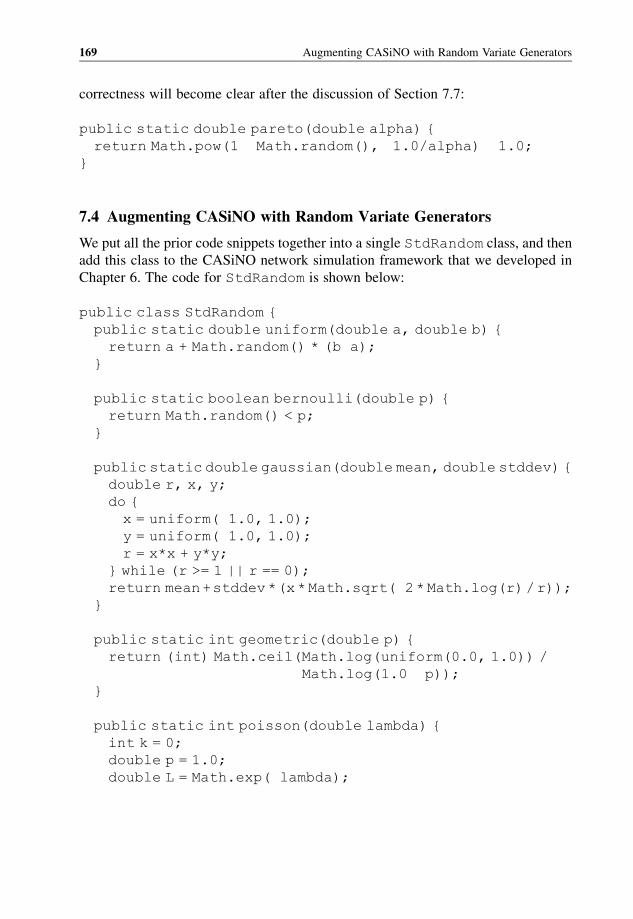
correctness will become clear after the discussion of Section 7.7:
public static double pareto(double alpha) {
return Math.pow(1 Math.random(), 1.0/alpha) 1.0;
}
7.4 Augmenting CASiNO with Random Variate Generators
We put all the prior code snippets together into a single StdRandom class, and then
add this class to the CASiNO network simulation framework that we developed in
Chapter 6. The code for StdRandom is shown below:
public class StdRandom {
public static double uniform(double a, double b) {
return a + Math.random() * (b a);
}
public static boolean bernoulli(double p) {
return Math.random() < p;
}
public static double gaussian(double mean, double stddev) {
double r, x, y;
do {
x = uniform( 1.0, 1.0);
y = uniform( 1.0, 1.0);
r = x*x + y*y;
} while (r >= 1 || r == 0);
return mean+stddev*(x*Math.sqrt( 2*Math.log(r)/r));
}
public static int geometric(double p) {
return (int) Math.ceil(Math.log(uniform(0.0, 1.0)) /
Math.log(1.0 p));
}
public static int poisson(double lambda) {
int k = 0;
double p = 1.0;
double L = Math.exp( lambda);
169 Augmenting CASiNO with Random Variate Generators

do {
k++;
p *= uniform(0.0, 1.0);
} while (p >= L);
return k 1;
}
public static double pareto(double alpha) {
return Math.pow(1 uniform(0.0, 1.0), 1.0/alpha) 1.0;
}
public static double exp(double lambda) {
return Math.log(1 Math.random()) / lambda;
}
}
7.5 Random Number Generation
Note that the code in all the prior distributions was built over the Math.random()
subroutine of Java. This shows that it is possible to generate most distributions given
access to a random variable that is uniformly distributed on the unit interval. Since
computers operate on finite precision representations of real numbers, this task
translates concretely to generating random n-bit integers (i.e., random integers in the
range of 0 . . . n). In this section, methods for the generation of such uniformly
distributed random integers are described, including the linear congruential method,
combined linear congruential method, and random number streams. Then, in
Section 7.6, tests of randomness, including frequency and correlations tests, will
be covered.
7.5.1 Linear Congruential Method
The linear congruential method produces a sequence of integers uniformly distributed
between 0 and m 1 following the recursive relationship:
Xiþ 1 ¼ ðaXi þ cÞmodm; i ¼ 0; 1; 2 . . . :
In this relationship a is called the multiplier, c is called the increment, m is the
modulus, and X0 is the seed. The parameters a, c, m, and X0 affect drastically the
statistical property and the cycle of the numbers.When c¼ 0, the form is known as the
multiplicative congruential method.
Statistical Distributions and Random Number Generation 170
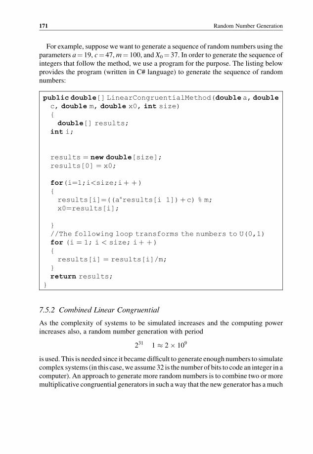
For example, supposewewant to generate a sequence of random numbers using the
parameters a¼ 19, c¼ 47,m¼ 100, and X0¼ 37. In order to generate the sequence of
integers that follow the method, we use a program for the purpose. The listing below
provides the program (written in C# language) to generate the sequence of random
numbers:
public double[] LinearCongruentialMethod(double a, doublec, double m, double x0, int size)
{
double[] results;
int i;
results ¼ new double[size];results[0] ¼ x0;
for(i¼1;i<size;iþ þ)
{
results[i]¼((a�results[i 1])þc) % m;
x0¼results[i];
}
//The following loop transforms the numbers to U(0,1)
for (i ¼ 1; i < size; iþ þ)
{
results[i] ¼ results[i]/m;
}
return results;
}
7.5.2 Combined Linear Congruential
As the complexity of systems to be simulated increases and the computing power
increases also, a random number generation with period
231 1 � 2� 109
is used. This is needed since it became difficult to generate enough numbers to simulate
complex systems (in this case,we assume32 is the number of bits to code an integer in a
computer). An approach to generate more random numbers is to combine two or more
multiplicative congruential generators in such away that the new generator has amuch
171 Random Number Generation
longer cycle. Later, a combined “linear congruential method” to generate random
numbers was proposed. In this method it is assumed that there is k multiplicative
congruential generators, where the jth generator has prime modulusmj and multiplier
aj. These are chosen in such away that the period ismj 1. The jth generator produces
random numbers Xi,j that are approximately uniformly distributed from 0 to m1 1.
The generator has the following form:
Xi ¼Xkj 1
ð 1Þj 1Xi;j
!modmi 1:
The maximum possible period for such a generator is given by:
P ¼ ðm1 1Þðm2 1Þ . . . ðmk 1Þ2k 1
:
7.5.3 Random Number Streams
As mentioned earlier, a linear congruential random number generator is character-
ized by the period m, the seed X0, a multiplier, and an increment. The sequence of
numbers generated using this method is repeated after the periodm. So, any number
in the sequence could be considered as the starting point or the seed of the sequence as
the generation is cyclic. The random number stream is a convenient way of referring
to the starting point and could take any value in the sequence. For a combined random
number generator, if the streams are b values apart, the stream i could be defined as
the starting seed Si¼Xb(i 1) such that i¼ 1, 2, . . ., P/b where P is the size of the
sample.
7.6 Frequency and Correlation Tests
The goal of random number generation schema is to produce a sequence of random
numbers that simulates the ideal properties. Each number returned must appear to be
chosen via the uniform distribution, and any two numbers must appear to have been
chosen independently. In order to test if a sequence of random numbers has these
proprieties, a set of tests needs to be performed. Tests of whether the distribution of the
set of randomnumber is uniformare frequently called frequency tests. Tests ofwhether
the generated numbers are independent of one another are called autocorrelation tests.
In what follows, we describe these two kinds of tests.
We begin with frequency tests; these are used to validate if a new random number
generator generates a uniform set of random numbers. The two most popular methods
that are available for such tests are the Kolmogorov–Smirnov and chi-square tests.
Statistical Distributions and Random Number Generation 172
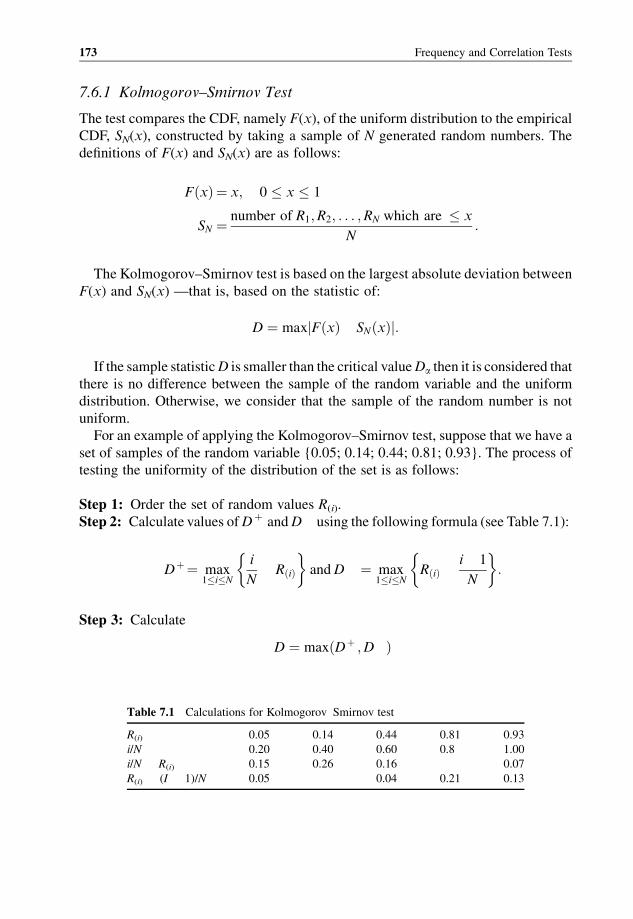
7.6.1 Kolmogorov–Smirnov Test
The test compares the CDF, namely F(x), of the uniform distribution to the empirical
CDF, SN(x), constructed by taking a sample of N generated random numbers. The
definitions of F(x) and SN(x) are as follows:
FðxÞ ¼ x; 0 � x � 1
SN ¼ number of R1;R2; . . . ;RN which are � x
N:
The Kolmogorov–Smirnov test is based on the largest absolute deviation between
F(x) and SN(x) —that is, based on the statistic of:
D ¼ maxjFðxÞ SNðxÞj:
If the sample statisticD is smaller than the critical valueDa then it is considered that
there is no difference between the sample of the random variable and the uniform
distribution. Otherwise, we consider that the sample of the random number is not
uniform.
For an example of applying the Kolmogorov–Smirnov test, suppose that we have a
set of samples of the random variable {0.05; 0.14; 0.44; 0.81; 0.93}. The process of
testing the uniformity of the distribution of the set is as follows:
Step 1: Order the set of random values R(i).
Step 2: Calculate values ofDþ andD using the following formula (see Table 7.1):
Dþ¼ max1�i�N
i
NRðiÞ
andD ¼ max
1�i�NRðiÞ
i 1
N
:
Step 3: Calculate
D ¼ maxðDþ ;D Þ
Table 7.1 Calculations for Kolmogorov Smirnov test
R(i) 0.05 0.14 0.44 0.81 0.93
i/N 0.20 0.40 0.60 0.8 1.00
i/N R(i) 0.15 0.26 0.16 0.07
R(i) (I 1)/N 0.05 0.04 0.21 0.13
173 Frequency and Correlation Tests
which yields D¼ 0.26. For a¼ 0.05 as the significance value and the number of
random values N¼ 5, compare D and Da. It is observed that Da¼ 0.565>D¼ 0.26.
Hence, the set of random values of the example are uniformly distributed.
7.6.2 Chi-Square Test
The chi-square test uses the following sample statistics:
w20 ¼Xni 1
ðOi EiÞ2Ei
where Oi is the observed number in the ith class, N is the total number of
observations, n is the number of classes, and Ei is the expected number in the ith
class given by:
Ei ¼ N
n:
If w20 is calculated using the above statistics and found to be smaller than the
theoretical critical value w2a;N such that a is the confidence level that can be accepted,the hypothesis is that the sample is uniformly distributed. Otherwise, the set of random
values is not considered as uniformly distributed.
7.6.3 Autocorrelation Tests
Autocorrelation tests are used to test if a set of random numbers is independent or
not. The test requires the computation of the autocorrelation between everym numbers
(m is the lag) starting with the ith number. So the autocorrelation between the set of
random numbers {Ri, Riþm, Riþ 2m, . . ., Riþ (Mþ 1)m} is rim such that N is the total
number in the sequence andM is the largest number such that iþðMþ 1Þm � N. The
non-zero autocorrelation implies a lack of independence. The test statistic
Z0 ¼ rim=srim is such that Z is normally distributed with a mean 0 and variance 1
and the formula for the estimators is:
rim ¼ 1
Mþ 1
XMk 0
Riþ kmRiþðkþ 1Þm
" #0:25
srim ¼ 13Mþ 7p
12ðMþ 1Þ :
Statistical Distributions and Random Number Generation 174
The autocorrelation test consists of calculating Z0 using the empirical distribution of
the sample of random numbers and comparing the result to the theoretical value taking
into consideration the significance level of the test. If Za=2 � Z0 � Za=2 where a isthe level of significance and Za/2 is obtained from the distribution table (found in any
statistics book), then it is considered that the set of random variable samples has been
generated independently.
7.7 Random Variate Generation
After specifying the distribution of the input random variables (Sections 7.2 and 7.3),
understanding how to generate random numbers uniformly at random (Section 7.4),
and validating their randomness (Section 7.5), we are now interested in generating
samples of the random numbers from a specified (non-uniform) distribution. We have
already presented Java codes for generating random samples from each of the discrete
and continuous distributions in Sections 7.2 and 7.3, but that code was presented
without justification. We now attempt to give the theoretical underpinnings justifying
that code.
The different methods of generating random variable samples include the inversion
method, the accept–reject method, and the importance sampling method.
7.7.1 Inversion Method
Thismethod could be used to sample randomnumbers using awide number of discrete
distributions. It is mostly used to generate samples from the exponential, the Weibull,
and the triangular distributions. The main steps of the inversion method are:
1. Generate a set of uniform random numbers such that R U(0,1).
2. Choose the CDF, F(x), of the random variable to be sampled.
3. Set F(X)¼R.
4. Solve the equation F(X)¼R for X in terms of R.
5. Generate the random variate Xi from Ri using the function R¼F 1(X).
As an example of the use of the inversion method, let us use the exponential
distribution. The CDF of the exponential distribution is:
FðxÞ ¼0 x < 0
1 e lx x � 0:
(
In order to generate randomnumberswith this distribution, we need to generate a set
of random number {Ri} using the uniform distribution. Then, we generate numbers Xi
175 Random Variate Generation

using the fact that the inverse of the CDF for the exponential distribution is:
F 1ðRiÞ ¼ 1
llogð1 RiÞ:
One simplification that is commonly used here is to replace (1 Ri) in the inverse
function by Ri since both numbers are uniformly distributed. Table 7.2 provides an
example of generating random variables using an exponential distribution with
mean 1.
Translating these ideas into a Java code, we get the previously stated Java code
which takes the arrival rate of the distribution as an argument and returns a
“double,” chosen according to the exponential distribution having the specified
arrival rate:
public static double exp(double lambda) {
return Math.log(1 Math.random()) / lambda;
}
7.7.2 Accept–Reject Method
Thismethod is used to generate random numbers using a statistical distribution. In this
method some of the generated random variables are accepted and others are rejected
based on a selection criterion. In the process of generating random numbers using this
method, it is assumed that there is a set of uniform random number Ri such that RU
(0, 1). There is also a statistical distribution function g(x) which generates random
variable X. Then, a function f is defined, which is chosen in the accept–reject method
such that f(x)� c � g(x) for all x, where c is a constant greater than 1. Themain steps of
the accept–reject method are:
1. Generate a set of uniform random numbers Ri.
2. Calculate a¼ f(X)/c � g(X).3. Generate the random numbers Yi using the g function (Yi¼ g(Ri)).
4. If Ri< a then accept Xi¼ Yi, otherwise reject Yi and go to step 3.
Table 7.2 Generation of exponential random numbers with l¼ 1
i 1 2 3 4 5
Ri 0.1306 0.0422 0.6597 0.7965 0.7696
Xi 0.1400 0.0431 1.078 1.592 1.468
Statistical Distributions and Random Number Generation 176
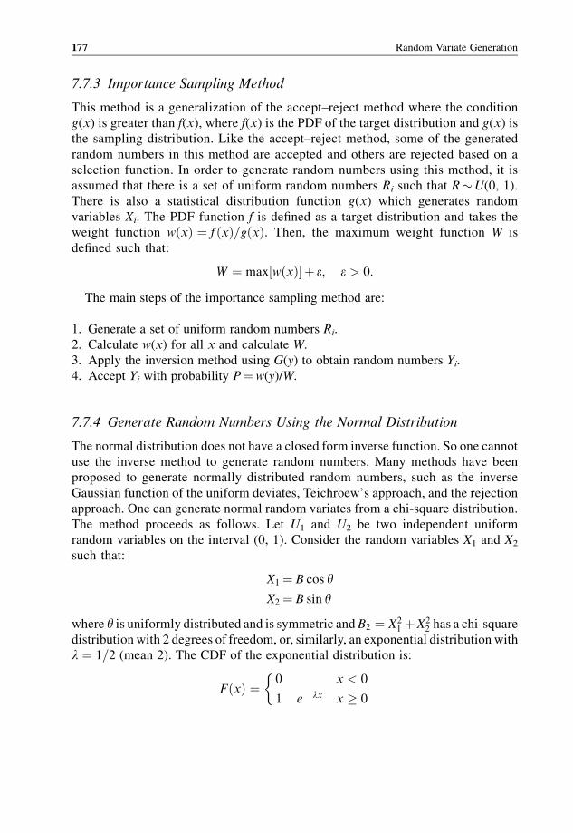
7.7.3 Importance Sampling Method
This method is a generalization of the accept–reject method where the condition
g(x) is greater than f(x), where f(x) is the PDF of the target distribution and g(x) is
the sampling distribution. Like the accept–reject method, some of the generated
random numbers in this method are accepted and others are rejected based on a
selection function. In order to generate random numbers using this method, it is
assumed that there is a set of uniform random numbers Ri such that RU(0, 1).
There is also a statistical distribution function g(x) which generates random
variables Xi. The PDF function f is defined as a target distribution and takes the
weight function wðxÞ ¼ f ðxÞ=gðxÞ. Then, the maximum weight function W is
defined such that:
W ¼ max½wðxÞ� þ e; e > 0:
The main steps of the importance sampling method are:
1. Generate a set of uniform random numbers Ri.
2. Calculate w(x) for all x and calculate W.
3. Apply the inversion method using G(y) to obtain random numbers Yi.
4. Accept Yi with probability P¼w(y)/W.
7.7.4 Generate Random Numbers Using the Normal Distribution
The normal distribution does not have a closed form inverse function. So one cannot
use the inverse method to generate random numbers. Many methods have been
proposed to generate normally distributed random numbers, such as the inverse
Gaussian function of the uniform deviates, Teichroew’s approach, and the rejection
approach. One can generate normal random variates from a chi-square distribution.
The method proceeds as follows. Let U1 and U2 be two independent uniform
random variables on the interval (0, 1). Consider the random variables X1 and X2
such that:
X1 ¼ B cos y
X2 ¼ B sin y
where y is uniformly distributed and is symmetric and B2 ¼ X21 þX2
2 has a chi-square
distribution with 2 degrees of freedom, or, similarly, an exponential distribution with
l ¼ 1=2 (mean 2). The CDF of the exponential distribution is:
FðxÞ ¼ 0 x < 0
1 e lx x � 0
177 Random Variate Generation
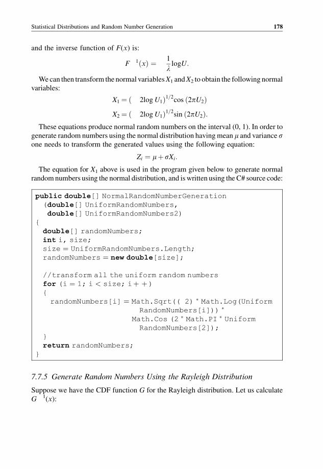
and the inverse function of F(x) is:
F 1ðxÞ ¼ 1
llogU:
Wecan then transform the normal variablesX1 andX2 to obtain the following normal
variables:
X1 ¼ ð 2logU1Þ1=2cos ð2pU2ÞX2 ¼ ð 2logU1Þ1=2sin ð2pU2Þ:
These equations produce normal random numbers on the interval (0, 1). In order to
generate random numbers using the normal distribution havingmean m and variance sone needs to transform the generated values using the following equation:
Zi ¼ mþ sXi:
The equation for X1 above is used in the program given below to generate normal
randomnumbers using the normal distribution, and is written using the C# source code:
public double[] NormalRandomNumberGeneration
(double[] UniformRandomNumbers,
double[] UniformRandomNumbers2)
{
double[] randomNumbers;
int i, size;
size ¼ UniformRandomNumbers.Length;
randomNumbers ¼ new double[size];
//transform all the uniform random numbers
for (i ¼ 1; i < size; iþ þ)
{
randomNumbers[i] ¼ Math.Sqrt(( 2) � Math.Log(UniformRandomNumbers[i])) �
Math.Cos (2 � Math.PI � UniformRandomNumbers[2]);
}
return randomNumbers;
}
7.7.5 Generate Random Numbers Using the Rayleigh Distribution
Suppose we have the CDF function G for the Rayleigh distribution. Let us calculate
G 1(x):
Statistical Distributions and Random Number Generation 178

LetGðXÞ ¼ R
) 1 expð X2=2s2Þ ¼ R
) expð X2=2s2Þ ¼ 1 R
) X2=2s2 ¼ lnð1 RÞ) X2 ¼ 2s2lnð1 RÞR 2 ½0; 1� lnð1 RÞ � 0
) X ¼ s 2 lnð1 RÞp:
Now, using the inverse method, we can derive the C# source code (given below) for
the generation of random numbers using the Rayleigh distribution:
public double[] Rayleigh(double[] UniformRandomNumbers,
double Sigma)
{
double[] randomNumbers;
int i, size;
size ¼ UniformRandomNumbers.Length;
randomNumbers ¼ new double[size];//transform all the uniform random numbers
for (i ¼ 1; i < size; iþ þ)
{
randomNumbers[i] ¼ Sigma � Math.Sqrt(( 2) �
Math.Log(1 UniformRandom
Numbers[i]));
}
return randomNumbers;
}
7.8 Summary
In this chapter, we have discussed a set of statistical distributions that could be used in
simulations as well as a set of random number generation techniques. An overview of
statistical distributions was presented first. Then discrete distributions were intro-
duced. Continuous distributions and discrete distributions were then discussed in
detail. Subsequently, a random number generator (RNG) was defined and its use in
simulations was presented.
179 Summary

Recommended Reading
[1] J. Banks, B. L. Nelson, J. S. Carson, D.M. Nicol, and J. CarsonII,Discrete event System Simulation,
5th Edition, Prentice Hall, 2009.
[2] L. Kleinrock, Queuing Systems: Computer Applications, Volume 2, John Wiley & Sons, Inc., 1975.
[3] S. Kotz, N. Balakrishnan, and N. L. Johnson, Continuous Multivariate Distributions, 2nd Edition,
Volume 2, John Wiley & Sons, Inc., 2000.
[4] N. L. Johnson, S. Kotz, and N. Balakrishnan, Discrete Multivariate Distributions, John Wiley
& Sons, Inc., 1997.
[5] S. Ross, A First Course in Probability, 4th Edition, Macmillan, 1994.
[6] D. S. Moore and G. McCabe, Introduction to the Practice of Statistics, 3rd Edition, WH Freeman,
1999.
[7] Online: http://www.ds.unifi.it/VL/VL EN/dist/dist4.html
Statistical Distributions and Random Number Generation 180
8
Network Simulation Elements:A Case Study Using CASiNO
In this chapter, we create some useful network simulation elements to serve as building
blocks in the network structures that wewill consider in the context of queuing theory
in Chapter 9. First, we will design and build a traffic generator which emits packets
according to a Poisson distribution. Then, we will design a protocol which processes
packets, taking a random amount of time to process each packet (with the processing
time being determined according to an exponential distribution). Later, we will see
how we can address the possibility of an infinite backlog in such a protocol.
Subsequently, we will develop an n-way round-robin multiplexer/demultiplexer.
Finally, we address the questions of dynamic instantiation and management of the
protocol conduits we developed earlier in the chapter.
8.1 Making a Poisson Source of Packets
In Tutorial 1 for CASiNO at the end of Chapter 6, we saw how to make a source of
PacketVisitors when we made a concrete conduit with adapter behavior by
specifying a terminal calledMySource. Now let us extend theMySource class so as
to make it a Poisson source of PacketVisitors. Here is the relevant code from
MySource for the constructor, and the recv() method:
public MySource() {
super();
send(this, new Tick(), 10.0);
}
Network Modeling and Simulation M. Guizani, A. Rayes, B. Khan and A. Al Fuqaha
� 2010 John Wiley & Sons, Ltd.

public void recv(SimEnt src, Event ev) {
if ((ev instanceof Tick) && ( a != null)) {
seqnum++;
a.inject(new PacketVisitor( seqnum, 0));
if ( seqnum < 10) {
send(this, ev, 10.0);
}
else {
Scheduler.instance().stop();
}
}
}
}
The original MySource has two data members of interest:
int recv = 0;
int seqnum = 0;
Now when we modify MySource to make it into a PoissonSource, we can
simply extend the class so that it will inherit all the common methods from its parent
class’s implementation:
public class PoissonSource extends MySource {
}
We need two new data members inside PoissonSource:
private int max;
private double lambda;
whose initial values will be passed as arguments to the constructor where they will
get set:
public PoissonSource(int numpackets, double lambda) {
super();
max=numpackets;
lambda=lambda;
}
Network Simulation Elements: A Case Study Using CASiNO 182

The recv() method of PoissonSource is modified to call the StdRandom
class’s static method poisson(), which was described at length in Chapter 7:
public void recv(SimEnt src, Event ev) {
if ((ev instanceof Tick) && ( a != null)) {
seqnum++;
a.inject(new PacketVisitor( seqnum, 0));
if ( seqnum < max) {
send(this, ev, StdRandom.poisson( lambda));
}
}
}
}
Note how the receipt of an event causes it to be scheduled for redelivery at a time that
is chosen according to the Poisson distribution.
8.2 Making a Protocol for Packet Processing
In Tutorial 3 of Chapter 6, we saw how to make a concrete conduit with protocol
behavior by specifying a state called MyStateMachine. It did very little. It counted
the PacketVisitors it received, passing on the first five through and killing all
subsequent PacketVisitors. Here is the relevant code from MyStateMachine
for its handle() method:
public boolean handle(Visitor v, Conduit.Side e) {
System.out.print(""+getName()+" received visitor "+v+
"attime"+Scheduler.getTime()+"...");
if (v instanceof PacketVisitor) {
counter++;
if ( counter>5) {
System.out.println("dropping");
dropped++;
return false;
}
else {
System.out.println("passing through");
passed++;
return true;
183 Making a Protocol for Packet Processing
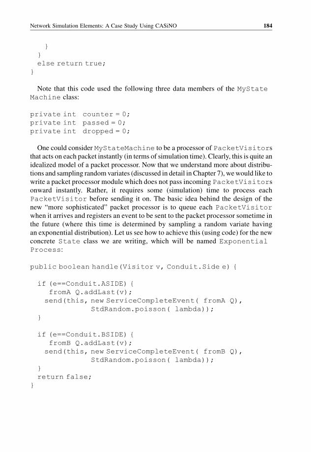
}
}
else return true;
}
Note that this code used the following three data members of the MyState
Machine class:
private int counter = 0;
private int passed = 0;
private int dropped = 0;
One could consider MyStateMachine to be a processor of PacketVisitors
that acts on each packet instantly (in terms of simulation time). Clearly, this is quite an
idealized model of a packet processor. Now that we understand more about distribu-
tions and sampling random variates (discussed in detail in Chapter 7), wewould like to
write a packet processor module which does not pass incoming PacketVisitors
onward instantly. Rather, it requires some (simulation) time to process each
PacketVisitor before sending it on. The basic idea behind the design of the
new “more sophisticated” packet processor is to queue each PacketVisitor
when it arrives and registers an event to be sent to the packet processor sometime in
the future (where this time is determined by sampling a random variate having
an exponential distribution). Let us see how to achieve this (using code) for the new
concrete State class we are writing, which will be named Exponential
Process:
public boolean handle(Visitor v, Conduit.Side e) {
if (e==Conduit.ASIDE) {
fromA Q.addLast(v);
send(this, new ServiceCompleteEvent( fromA Q),
StdRandom.poisson( lambda));
}
if (e==Conduit.BSIDE) {
fromB Q.addLast(v);
send(this, new ServiceCompleteEvent( fromB Q),
StdRandom.poisson( lambda));
}
return false;
}
Network Simulation Elements: A Case Study Using CASiNO 184
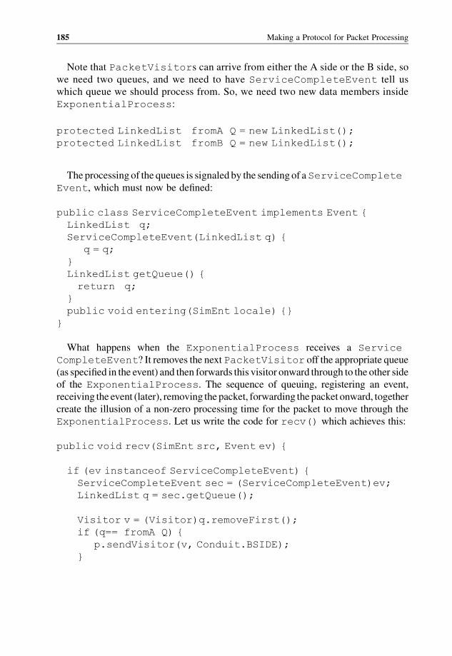
Note that PacketVisitors can arrive from either the A side or the B side, so
we need two queues, and we need to have ServiceCompleteEvent tell us
which queue we should process from. So, we need two new data members inside
ExponentialProcess:
protected LinkedList fromA Q = new LinkedList();
protected LinkedList fromB Q = new LinkedList();
The processing of the queues is signaled by the sending of aServiceComplete
Event, which must now be defined:
public class ServiceCompleteEvent implements Event {
LinkedList q;
ServiceCompleteEvent(LinkedList q) {
q = q;
}
LinkedList getQueue() {
return q;
}
public void entering(SimEnt locale) {}
}
What happens when the ExponentialProcess receives a Service
CompleteEvent? It removes the nextPacketVisitor off the appropriate queue
(as specified in the event) and then forwards this visitor onward through to the other side
of the ExponentialProcess. The sequence of queuing, registering an event,
receiving the event (later), removing the packet, forwarding the packet onward, together
create the illusion of a non-zero processing time for the packet to move through the
ExponentialProcess. Let us write the code for recv() which achieves this:
public void recv(SimEnt src, Event ev) {
if (ev instanceof ServiceCompleteEvent) {
ServiceCompleteEvent sec = (ServiceCompleteEvent)ev;
LinkedList q = sec.getQueue();
Visitor v = (Visitor)q.removeFirst();
if (q== fromA Q) {
p.sendVisitor(v, Conduit.BSIDE);
}
185 Making a Protocol for Packet Processing
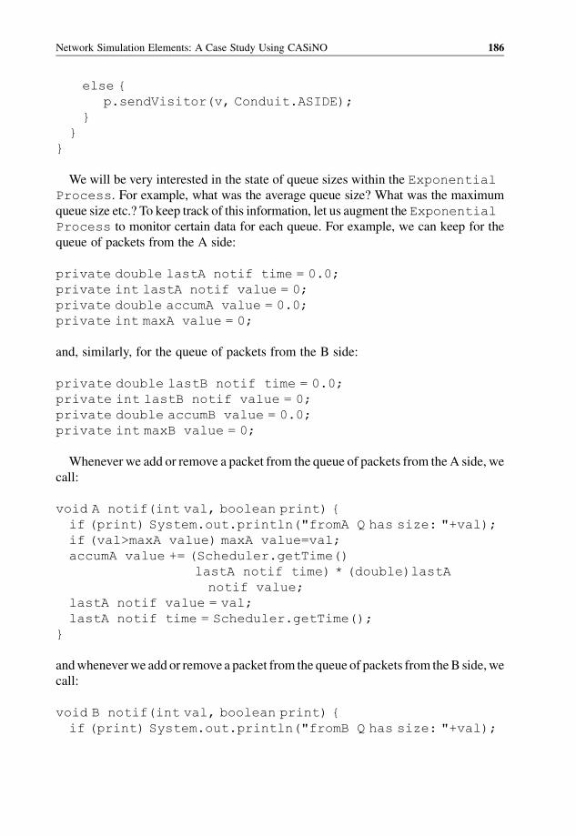
else {
p.sendVisitor(v, Conduit.ASIDE);
}
}
}
We will be very interested in the state of queue sizes within the Exponential
Process. For example, what was the average queue size? What was the maximum
queue size etc.? To keep track of this information, let us augment the Exponential
Process to monitor certain data for each queue. For example, we can keep for the
queue of packets from the A side:
private double lastA notif time = 0.0;
private int lastA notif value = 0;
private double accumA value = 0.0;
private int maxA value = 0;
and, similarly, for the queue of packets from the B side:
private double lastB notif time = 0.0;
private int lastB notif value = 0;
private double accumB value = 0.0;
private int maxB value = 0;
Whenever we add or remove a packet from the queue of packets from the A side, we
call:
void A notif(int val, boolean print) {
if (print) System.out.println("fromA Q has size: "+val);
if (val>maxA value) maxA value=val;
accumA value += (Scheduler.getTime()
lastA notif time) * (double)lastA
notif value;
lastA notif value = val;
lastA notif time = Scheduler.getTime();
}
andwheneverwe add or remove a packet from the queue of packets from theB side, we
call:
void B notif(int val, boolean print) {
if (print) System.out.println("fromB Q has size: "+val);
Network Simulation Elements: A Case Study Using CASiNO 186

if (val>maxB value) maxB value=val;
accumB value += (Scheduler.getTime()
lastB notif time) * (double)lastB
notif value;
lastB notif value = val;
lastB notif time = Scheduler.getTime();
}
These methods maintain the local statistical information about the mean and
maximum size of the queues (from both the A side and the B side). Then, we
need somemethods to get these performance measurements for the Exponential
Process instance:
public double max fromA Qsize() {
return maxA value;
}
public double max fromB Qsize() {
return maxB value;
}
public double mean fromA Qsize() {
A notif(lastA notif value, false);
return accumA value/lastA notif time;
}
public double mean fromB Qsize() {
B notif(lastB notif value, false);
return accumB value/lastB notif time;
}
8.3 Bounding Protocol Resources
In the previous section, we saw how to make a packet processor as a concrete state
specifying a protocol behavior. This new packet processor, the Exponential
Process, used two queues, one for packets flowing in from the A side and one for
packets flowing in from the B side. Both of these queues could grow arbitrarily
large, however. Clearly, this was a very idealized model. Here we extend this
model, making it a more realistic class that bounds the size of these queues. In
short, the new class, which we will name ExponentialBoundedProcess,
will take an additional argument, the maximum queue size. If at any point, adding a
187 Bounding Protocol Resources
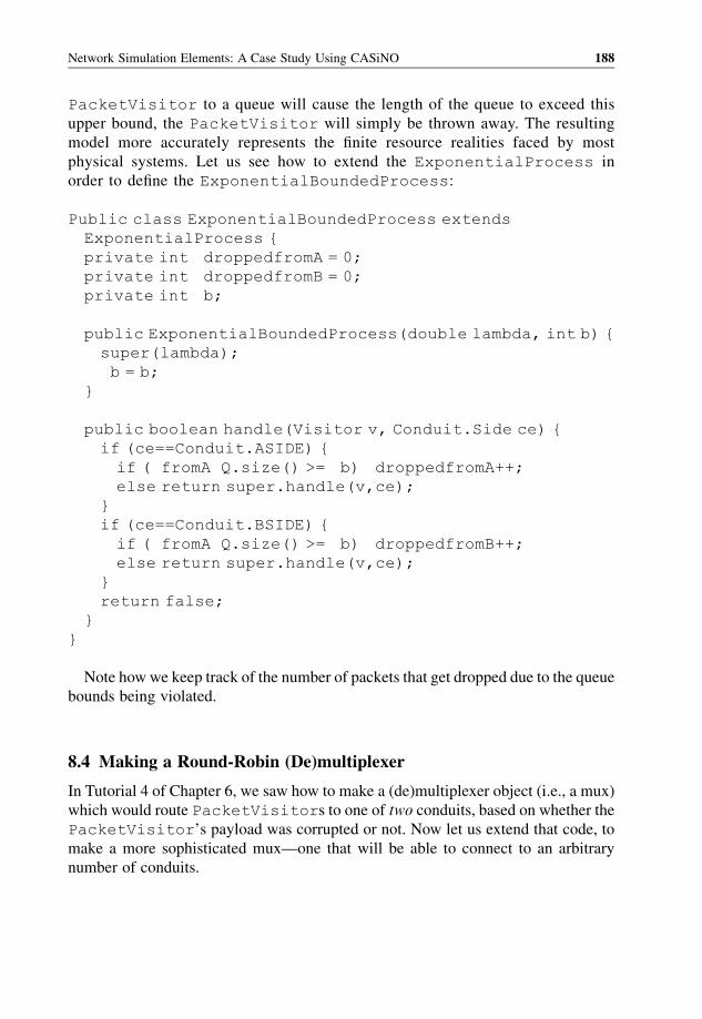
PacketVisitor to a queue will cause the length of the queue to exceed this
upper bound, the PacketVisitor will simply be thrown away. The resulting
model more accurately represents the finite resource realities faced by most
physical systems. Let us see how to extend the ExponentialProcess in
order to define the ExponentialBoundedProcess:
Public class ExponentialBoundedProcess extends
ExponentialProcess {
private int droppedfromA = 0;
private int droppedfromB = 0;
private int b;
public ExponentialBoundedProcess(double lambda, int b) {
super(lambda);
b = b;
}
public boolean handle(Visitor v, Conduit.Side ce) {
if (ce==Conduit.ASIDE) {
if ( fromA Q.size() >= b) droppedfromA++;
else return super.handle(v,ce);
}
if (ce==Conduit.BSIDE) {
if ( fromA Q.size() >= b) droppedfromB++;
else return super.handle(v,ce);
}
return false;
}
}
Note how we keep track of the number of packets that get dropped due to the queue
bounds being violated.
8.4 Making a Round-Robin (De)multiplexer
In Tutorial 4 of Chapter 6, we saw how to make a (de)multiplexer object (i.e., a mux)
which would route PacketVisitors to one of two conduits, based on whether the
PacketVisitor’s payload was corrupted or not. Now let us extend that code, to
make a more sophisticated mux—one that will be able to connect to an arbitrary
number of conduits.
Network Simulation Elements: A Case Study Using CASiNO 188

Our new mux (which we call RoundRobin) should forward PacketVisitors
coming in from its A side in a cyclical manner to each of the conduits that have been
connected to its B side. This is the demultiplexing behavior. It should forward
PacketVisitors coming in from any conduit on its B side to the one conduit
on its A side. This is the multiplexing behavior. In order to do this, we need to specify
the accessor which is used to route visitors to and join conduits to the B side.
RoundRobin will need two data members to keep track of its neighboring conduits
on the B side:
private HashMap port2protocol = new HashMap();
private int m=0;
Here the value of m will always be the number of neighbors on the B side. To
achieve round-robin routing, we need to define the getNextConduit() method,
since this is consulted by the mux behavior code to determine where to send visitors
which enter from the A side:
private int index = 0;
private int n = 0;
public Conduit.Half getNextConduit(Visitor v) {
if (v instanceof PacketVisitor) {
Conduit.Half ce = (Conduit.Half)
port2protocol.get(new Integer( index));
index = ( index+1) % m;
n++;
return ce;
}
else return null;
}
Finally, to support dynamically binding conduits to theB side, let us introduce a new
kind of visitor called the InitializeVisitor, which will specify the key (or ID)
to associate with the newly attached conduit. To attach a conduit to the B side of
RoundRobin, we would then call:
public void setNextConduit(Visitor v, Conduit.Half ce) {
int id = ((InitializeVisitor)v). id;
port2protocol.put( new Integer(id), ce);
m = port2protocol.size();
}
189 Making a Round Robin (De)multiplexer
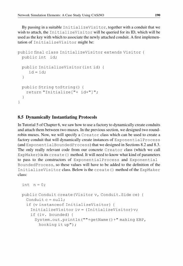
By passing in a suitable InitializeVisitor, together with a conduit that we
wish to attach, the InitializeVisitor will be queried for its ID, which will be
used as the key with which to associate the newly attached conduit. A first implemen-
tation of InitializeVisitor might be:
public final class InitializeVisitor extends Visitor {
public int id;
public InitializeVisitor(int id) {
id = id;
}
public String toString() {
return "Initialize["+ id+"]";
}
}
8.5 Dynamically Instantiating Protocols
In Tutorial 5 of Chapter 6, we saw how to use a factory to dynamically create conduits
and attach them between two muxes. In the previous section, we designed two round-
robin muxes. Now, we will specify a Creator class which can be used to create a
factory conduit that will dynamically create instances of ExponentialProcess
(and ExponentialBoundedProcess) that we designed in Sections 8.2 and 8.3.
The only really relevant code from our concrete Creator class (which we call
ExpMaker) is its create()method. It will need to know what kind of parameters
to pass to the constructors of ExponentialProcess and Exponential
BoundedProcess, so these values will have to be added to the definition of the
InitializeVisitor class. Below is the create()method of the ExpMaker
class:
int n = 0;
public Conduit create(Visitor v, Conduit.Side ce) {
Conduit c = null;
if (v instanceof InitializeVisitor) {
InitializeVisitor iv = (InitializeVisitor)v;
if (iv. bounded) {
System.out.println(""+getName()+" making EBP,
hooking it up");
Network Simulation Elements: A Case Study Using CASiNO 190
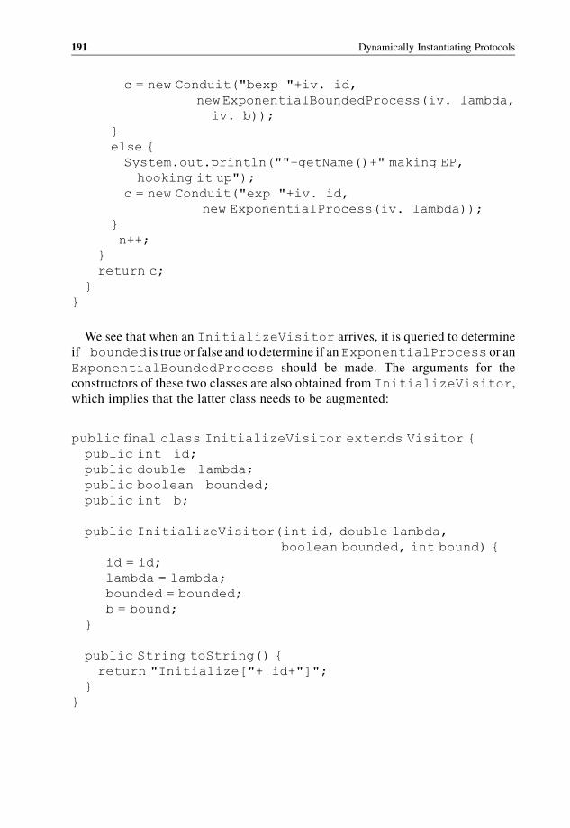
c = new Conduit("bexp "+iv. id,
newExponentialBoundedProcess(iv. lambda,
iv. b));
}
else {
System.out.println(""+getName()+" making EP,
hooking it up");
c = new Conduit("exp "+iv. id,
new ExponentialProcess(iv. lambda));
}
n++;
}
return c;
}
}
We see that when an InitializeVisitor arrives, it is queried to determine
if bounded is true or false and to determine if an ExponentialProcess or an
ExponentialBoundedProcess should be made. The arguments for the
constructors of these two classes are also obtained from InitializeVisitor,
which implies that the latter class needs to be augmented:
public final class InitializeVisitor extends Visitor {
public int id;
public double lambda;
public boolean bounded;
public int b;
public InitializeVisitor(int id, double lambda,
boolean bounded, int bound) {
id = id;
lambda = lambda;
bounded = bounded;
b = bound;
}
public String toString() {
return "Initialize["+ id+"]";
}
}
191 Dynamically Instantiating Protocols
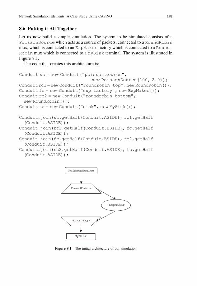
8.6 Putting it All Together
Let us now build a simple simulation. The system to be simulated consists of a
PoissonSource which acts as a source of packets, connected to a RoundRobin
mux, which is connected to an ExpMaker factory which is connected to a Round
Robin mux which is connected to a MySink terminal. The system is illustrated in
Figure 8.1.
The code that creates this architecture is:
Conduit sc = new Conduit("poisson source",
new PoissonSource(100, 2.0));
Conduitrc1=newConduit("roundrobin top",newRoundRobin());
Conduit fc = new Conduit("exp factory", new ExpMaker());
Conduit rc2 = new Conduit("roundrobin bottom",
new RoundRobin());
Conduit tc = new Conduit("sink", new MySink());
Conduit.join(sc.getHalf(Conduit.ASIDE), rc1.getHalf
(Conduit.ASIDE));
Conduit.join(rc1.getHalf(Conduit.BSIDE), fc.getHalf
(Conduit.ASIDE));
Conduit.join(fc.getHalf(Conduit.BSIDE), rc2.getHalf
(Conduit.BSIDE));
Conduit.join(rc2.getHalf(Conduit.ASIDE), tc.getHalf
(Conduit.ASIDE));
RoundRobin
RoundRobin
MySink
ExpMaker
PoissonSource
Figure 8.1 The initial architecture of our simulation
Network Simulation Elements: A Case Study Using CASiNO 192
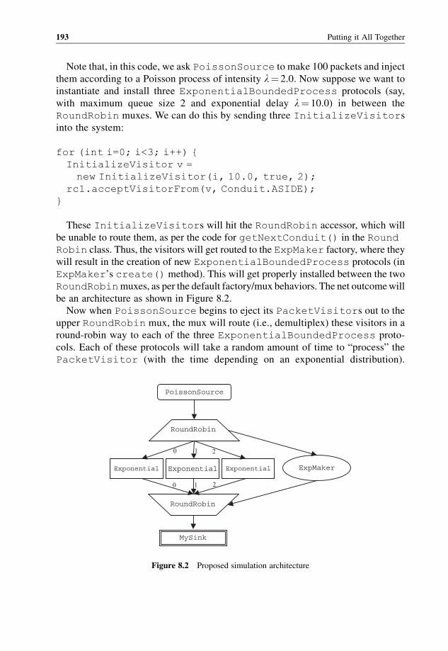
Note that, in this code, we ask PoissonSource to make 100 packets and inject
them according to a Poisson process of intensity l¼ 2.0. Now suppose we want to
instantiate and install three ExponentialBoundedProcess protocols (say,
with maximum queue size 2 and exponential delay l¼ 10.0) in between the
RoundRobin muxes. We can do this by sending three InitializeVisitors
into the system:
for (int i=0; i<3; i++) {
InitializeVisitor v =
new InitializeVisitor(i, 10.0, true, 2);
rc1.acceptVisitorFrom(v, Conduit.ASIDE);
}
These InitializeVisitors will hit the RoundRobin accessor, which will
be unable to route them, as per the code for getNextConduit() in the Round
Robin class. Thus, the visitors will get routed to the ExpMaker factory, where they
will result in the creation of new ExponentialBoundedProcess protocols (in
ExpMaker’s create() method). This will get properly installed between the two
RoundRobinmuxes, as per the default factory/mux behaviors. The net outcomewill
be an architecture as shown in Figure 8.2.
Now when PoissonSource begins to eject its PacketVisitors out to the
upper RoundRobin mux, the mux will route (i.e., demultiplex) these visitors in a
round-robin way to each of the three ExponentialBoundedProcess proto-
cols. Each of these protocols will take a random amount of time to “process” the
PacketVisitor (with the time depending on an exponential distribution).
RoundRobin
RoundRobin
MySink
ExpMakerExponential ExponentialExponential
1 0 2
1 0 2
PoissonSource
Figure 8.2 Proposed simulation architecture
193 Putting it All Together
Having processed the PacketVisitor, each ExponentialBounded
Process protocol will forward the visitor to the lower RoundRobin mux,
which will route the visitors (i.e., multiplex) to the MySink terminal.
Let us look at the output of a sample execution of this system, which asks
PoissonSource to make 100 packets and inject them according to a Poisson
process of intensity l¼ 2.0:
exp factory making EBP, hooking it up
bexp 0 received visitor Initialize[0] at time 0.0 ... fromA Q
has size: 1
exp factory making EBP, hooking it up
bexp 1 received visitor Initialize[1] at time 0.0 ... fromA Q
has size: 1
exp factory making EBP, hooking it up
bexp 2 received visitor Initialize[2] at time 0.0 ... fromA Q
has size: 1
sink received visitor Initialize[1] at time 7.0
bexp 0 received visitor Packet[1]:0:(0) at time 10.0 ...
fromA Q has size: 2
sink received visitor Initialize[0] at time 11.0
bexp 1 received visitor Packet[2]:0:(0) at time 12.0 ...
fromA Q has size: 1
bexp 2 received visitor Packet[3]:0:(0) at time 13.0 ...
fromA Q has size: 2
bexp 0 received visitor Packet[4]:0:(0) at time 14.0 ...
fromA Q has size: 2
sink received visitor Initialize[2] at time 15.0
bexp 1 received visitor Packet[5]:0:(0) at time 17.0 ...
fromA Q has size: 2
sink received visitor Packet[2]:0:(0) at time 19.0
<many lines of output>
bexp 0 received visitor Packet[97]:0:(0) at time 215.0 ...
fromA Q has size: 2
bexp 1 received visitor Packet[98]:0:(0) at time 219.0 ...
fromA Q has size: 1
bexp 2 received visitor Packet[99]:0:(0) at time 219.0 ...
fromA Q has size: 2
sink received visitor Packet[91]:0:(0) at time 220.0
Network Simulation Elements: A Case Study Using CASiNO 194
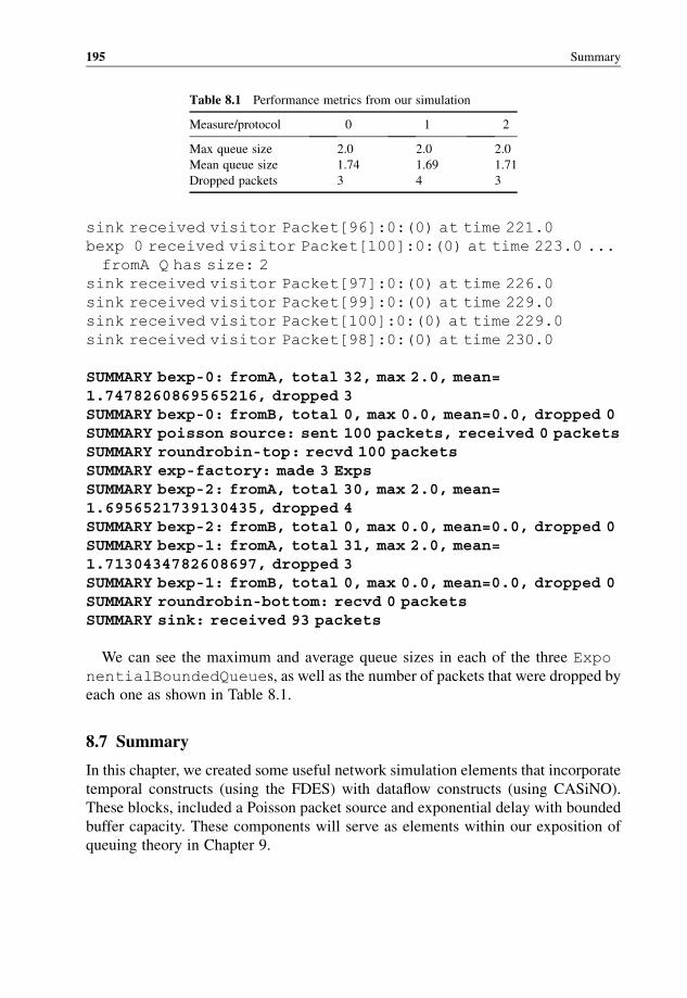
sink received visitor Packet[96]:0:(0) at time 221.0
bexp 0 received visitor Packet[100]:0:(0) at time 223.0 ...
fromA Q has size: 2
sink received visitor Packet[97]:0:(0) at time 226.0
sink received visitor Packet[99]:0:(0) at time 229.0
sink received visitor Packet[100]:0:(0) at time 229.0
sink received visitor Packet[98]:0:(0) at time 230.0
SUMMARY bexp-0: fromA, total 32, max 2.0, mean=1.7478260869565216, dropped 3SUMMARY bexp-0: fromB, total 0, max 0.0, mean=0.0, dropped 0SUMMARY poisson source: sent 100 packets, received 0 packetsSUMMARY roundrobin-top: recvd 100 packetsSUMMARY exp-factory: made 3 ExpsSUMMARY bexp-2: fromA, total 30, max 2.0, mean=1.6956521739130435, dropped 4SUMMARY bexp-2: fromB, total 0, max 0.0, mean=0.0, dropped 0SUMMARY bexp-1: fromA, total 31, max 2.0, mean=1.7130434782608697, dropped 3SUMMARY bexp-1: fromB, total 0, max 0.0, mean=0.0, dropped 0SUMMARY roundrobin-bottom: recvd 0 packetsSUMMARY sink: received 93 packets
We can see the maximum and average queue sizes in each of the three Expo
nentialBoundedQueues, as well as the number of packets that were dropped by
each one as shown in Table 8.1.
8.7 Summary
In this chapter, we created some useful network simulation elements that incorporate
temporal constructs (using the FDES) with dataflow constructs (using CASiNO).
These blocks, included a Poisson packet source and exponential delay with bounded
buffer capacity. These components will serve as elements within our exposition of
queuing theory in Chapter 9.
Table 8.1 Performance metrics from our simulation
Measure/protocol 0 1 2
Max queue size 2.0 2.0 2.0
Mean queue size 1.74 1.69 1.71
Dropped packets 3 4 3
195 Summary

9
Queuing Theory
Queuing theory is important in simulations because it provides theoretical predictions
against which to validate simulation results. In other words, often a simulation model
may be simplified so that queuing theory may be applied to yield theoretical
predictions. These predictions are then compared to the experimental measurements
obtained through computation to give some assurance of the validity of the simulation
implementation.
This chapter presents a brief discussion on several topics of queuing theory. In the
first part, basic conceptswill be covered. In the second part, specific practical caseswill
be presented and discussed. Whenever possible, there will be code samples imple-
mented using the CASiNO framework (developed in Chapters 6 and 8), the SimJava
Package, or MATLAB. It is expected that the reader is familiar with SimJava and
MATLAB in order to follow the examples which will appear later in this chapter.
In the first part of the chapter, the following topics will be covered:
. Introduction to stochastic processes
. Discrete-time and continuous-time Markov chains
. Some properties of Markov chains
. Chapman–Kolmogorov equation (C–K equation)
. Birth–death process (BD process).
Then, in the second part, we will cover:
. Little’s theorem
. The exponential distribution
. The Poisson process
. Standard notation of queuing systems
Network Modeling and Simulation M. Guizani, A. Rayes, B. Khan and A. Al Fuqaha
� 2010 John Wiley & Sons, Ltd.
. M/M/1 queue
. M/M/n queue
. M/M/1/b queue
. M/M/m/m queue.
9.1 Introduction to Stochastic Processes
A stochastic process (or a random process) is a family of random variables
indexed by an ordered set T, formally expressible as {X(t), t2 T}. That is, for any
fixed t in T, X(t) is a random variable. A stochastic process is the counterpart to a
deterministic system in probability theory. Instead of dealing with only one
possible event determining how the system might evolve over time, in stochastic
processes there is some indeterminacy in its future evolution (the values of X(t) for
higher values of t in T)—though this indeterminacy is quantifiable with probability
distributions. Stochastic processes are classified in different ways, such as by
index set, and by the state space, or the “set of all possible values that the random
variables X(t) can assume.” The following are a few examples of the different
cases that can occur.
Example 1 LetW be the amount of time that elapses from the arrival of amessage till
the processing begins, {W(t), t� 0}. The randomvariable is indexed by the arrival time
of the message (t), which is a continuous parameter, and the state space ofW(t) is also
continuous since the waiting time can be any real non-negative number.
Example 2 LetXn, n¼ {3.2, 2.1, 5.0, 4.3, 7.77, 1.2, 6.44}, denote the average time to
run a job at a computer center on the nth day of the week. That is, X1 is the average job
time on day 1: Sunday; X2 is the average job time on day 2: Monday; and so on. Then
{Xn} is a discrete set, though the state space is continuous.
Example 3 If the number of packets (P) in a queue of messages at the time when a
message arrives is {P(t), t� 0}, then the random variable is indexed by the arrival time
of the message (t). This is considered to be a continuous parameter and the state space
is discrete, since the number of messages in the queue is always an integer.
Example 4 Let Xn, n¼ {0, 2, 5, 4, 7, 1, 0}, denote the number of cars that passed
through checkpoint A on the nth day of the week. That is, X1 is the number on day 1:
Sunday;X2 is the number on day 2:Monday; and so on. Then {Xn} is a discrete set, and
the state space is discrete as well. Figure 9.1 shows the different cases that could arise
as random variables.
Queuing Theory 198

A random process can be used to generate graphs of natural events, like the amount
of rainfall as a function of the index variable, time. A hypothetical graph showing how
much rain fell in the city of Chicago during 2006 with index variable 1� t� 365 days
is shown in Figure 9.2.
W(t)Continuous Time,Continuous Value Process
X(t)Discrete Time,Continuous Value Process
Y(t)Continuous Time,Discrete Value Process
Z(t)Discrete Time,Discrete Value Process
Figure 9.1 Different cases of random variables
f (t,Y)
Figure 9.2 Rainfall in Chicago during 2006 (1� t� 365 days)
199 Introduction to Stochastic Processes
If there are only countably many times (i.e., values of the index variable) at
which the random variable can change its value, the random process is called a
discrete parameter process Xn. If these changes occur anywhere within a continu-
ous interval, we have a continuous parameter process X(t); we often write Xn to
refer to a random or stochastic sequence and X(t) to a stochastic or random
process.
The most common types of stochastic processes that appear in the context of
simulation studies are listed below. They are characterized by different kinds of
dependency relations among their constituent random variables. This classification
provides a global overview of the different sub-branches within the field of queuing
theory.
. Independent processes: These are the simplest andmost trivial. They consider the
sequence in which {Xn} forms a set of independent random variables.. Markov processes: A set of random variables, say {Xn}, forms a Markov chain if
the probability that the next state is Xnþ 1 depends only upon the current stateXn and
not upon any earlier values.. Birth–death processes: AMarkov process with discrete state space, whose states
can be enumerated with an index, say i¼ 0, 1, 2 . . . such that the state transitions
occur only between neighboring states.. Semi-Markov processes: These extend the notion of Markov processes by allow-
ing the time between state transitions to obey an arbitrary probability distribution.
The case when a transition must be made at every unit time is the classical Markov
process, in which the time spent in one state is geometrically distributed.. Random walks: Can be thought of as an object moving among states in some
state space (e.g., discrete space). A location of this object is defined in a certain
state.. Stationary processes: A stochastic process X(t) is said to be stationary if there is a
Fx(x; t) which is invariant to the shifts in time for all values of its arguments.
A Markov process with a discrete state space is referred to as aMarkov chain. A
set of random variables, say {Xn}, forms a Markov chain if the probability that the
next state is Xnþ 1 depends only upon the current state Xn and not upon any previous
values. This also implies that the probability distribution of Xn (denoted Pn)
depends only on the previous state and no earlier Xi (for i< n 1). In short, we
have a random sequence in which the dependency is extended backward at most
one unit in time.
Consider a stochastic process {X(t), t2 T}. This stochastic process is called a
Markov process if for any increasing sequence of n þ 1 values of (say time) t such that
t1< t2< t3< � � � < tn< tnþ 1 in the index set, and any set {x1, x2, x3, . . ., xnþ 1} of
Queuing Theory 200
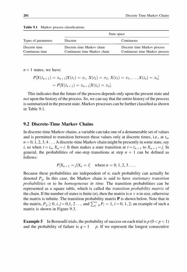
nþ 1 states, we have:
P½Xðtnþ 1Þ ¼ xnþ 1jXðt1Þ ¼ x1; Xðt2Þ ¼ x2; Xðt3Þ ¼ x3; . . . ;XðtnÞ ¼ xn�¼ P½Xðtnþ 1Þ ¼ xnþ 1jXðtnÞ ¼ xn�:
This indicates that the future of the process depends only upon the present state and
not upon the history of the process. So, we can say that the entire history of the process
is summarized in the present state.Markov processes can be further classified as shown
in Table 9.1.
9.2 Discrete-Time Markov Chains
In discrete-timeMarkov chains, a variable can take one of a denumerable set of values
and is permitted to transition between these values only at discrete times, i.e., at tn,
n¼ 0, 1, 2, 3, 4 . . .. A discrete-timeMarkov chainmight be presently in some state, say
i, so when t¼ tn, Xn¼ i. It then makes a state transition at t¼ tnþ 1 to Xnþ 1¼ j. In
general, the probabilities of one-step transitions at step n þ 1 can be defined as
follows:
P½Xnþ 1 ¼ jjXn ¼ i� where n ¼ 0; 1; 2; 3 . . . :
Because these probabilities are independent of n, each probability can actually be
denoted Pij. In this case, the Markov chain is said to have stationary transition
probabilities or to be homogeneous in time. The transition probabilities can be
represented as a square table, which is called the transition probability matrix of
the chain. If the number of states is finite (n), then the matrix is n� n in size, otherwise
the matrix is infinite. The transition probability matrix P is shown below. Note that in
the matrix, Pij� 0, i, j¼ 0,1, 2 . . ., andP¥
j 0 Pi ¼ 1, i¼ 0, 1, 2; an example of such a
matrix is shown in Figure 9.3.
Example 5 In Bernoulli trials, the probability of success on each trial is p (0< p< 1)
and the probability of failure is q¼ 1 p. If we represent the longest consecutive
Table 9.1 Markov process classifications
State space
Types of parameters Discrete Continuous
Discrete time Discrete time Markov chain Discrete time Markov process
Continuous time Continuous time Markov chain Continuous time Markov process
201 Discrete Time Markov Chains
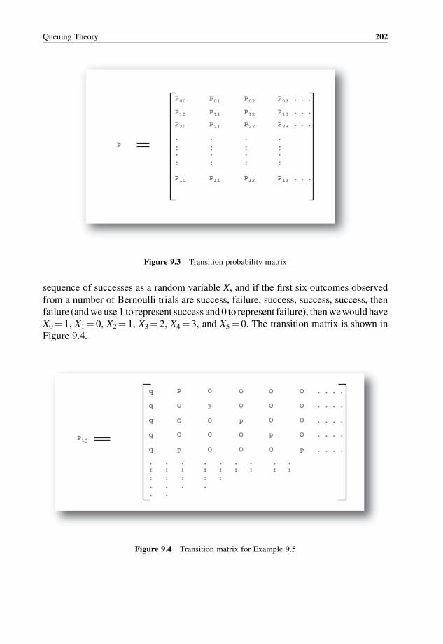
sequence of successes as a random variable X, and if the first six outcomes observed
from a number of Bernoulli trials are success, failure, success, success, success, then
failure (andweuse 1 to represent success and 0 to represent failure), thenwewould have
X0¼ 1, X1¼ 0, X2¼ 1, X3¼ 2, X4¼ 3, and X5¼ 0. The transition matrix is shown in
Figure 9.4.
P00
P
P01 P02 P03 . . .
. . .
. . .
. . .
P13
P23
P13
P12
P22
P12
P11
P21
P11
P10
P20
.
..
.
..
.
..
.
..
.
..
.
..
.
..
.
..
P10
Figure 9.3 Transition probability matrix
q P
O
O
P
O
O
O O
O
P
O
O O
O
O
O . . . .
. . . .
. . . .
. . . .
. . . .
O
O
O
PO
P
O
O
P
Pij
q
q
q
q
.
..
..
.
.
.
..
..
.
.
.
..
..
.
.
..
..
.
..
.
.
.....
.
.....
..
Figure 9.4 Transition matrix for Example 9.5
Queuing Theory 202
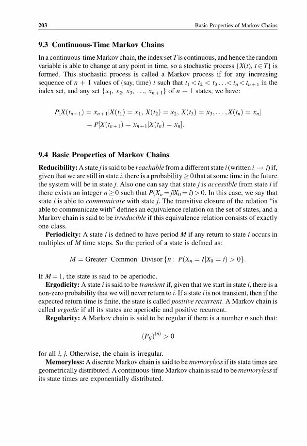
9.3 Continuous-Time Markov Chains
In a continuous-timeMarkov chain, the index setT is continuous, and hence the random
variable is able to change at any point in time, so a stochastic process {X(t), t2 T} is
formed. This stochastic process is called a Markov process if for any increasing
sequence of n þ 1 values of (say, time) t such that t1< t2 < t3 . . .< tn< tnþ 1 in the
index set, and any set {x1, x2, x3, . . ., xnþ 1} of n þ 1 states, we have:
P½Xðtnþ 1Þ ¼ xnþ 1jXðt1Þ ¼ x1; Xðt2Þ ¼ x2; Xðt3Þ ¼ x3; . . . ;XðtnÞ ¼ xn�¼ P½Xðtnþ 1Þ ¼ xnþ 1jXðtnÞ ¼ xn�:
9.4 Basic Properties of Markov Chains
Reducibility:Astate j is said to be reachable from a different state i (written i ! j) if,
given that we are still in state i, there is a probability� 0 that at some time in the future
the system will be in state j. Also one can say that state j is accessible from state i if
there exists an integer n� 0 such that P(Xn¼ j|X0¼ i)> 0. In this case, we say that
state i is able to communicate with state j. The transitive closure of the relation “is
able to communicate with” defines an equivalence relation on the set of states, and a
Markov chain is said to be irreducible if this equivalence relation consists of exactly
one class.
Periodicity: A state i is defined to have period M if any return to state i occurs in
multiples of M time steps. So the period of a state is defined as:
M ¼ Greater Common Divisor fn : PðXn ¼ IjX0 ¼ iÞ > 0g:
If M¼ 1, the state is said to be aperiodic.
Ergodicity:A state i is said to be transient if, given that we start in state i, there is a
non-zero probability that wewill never return to i. If a state i is not transient, then if the
expected return time is finite, the state is called positive recurrent. A Markov chain is
called ergodic if all its states are aperiodic and positive recurrent.
Regularity: A Markov chain is said to be regular if there is a number n such that:
ðPijÞðnÞ > 0
for all i, j. Otherwise, the chain is irregular.
Memoryless:AdiscreteMarkov chain is said to bememoryless if its state times are
geometrically distributed. A continuous-timeMarkov chain is said to bememoryless if
its state times are exponentially distributed.
203 Basic Properties of Markov Chains
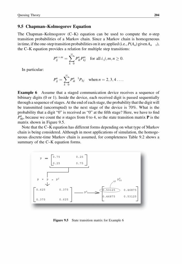
9.5 Chapman–Kolmogorov Equation
The Chapman–Kolmogorov (C–K) equation can be used to compute the n-step
transition probabilities of a Markov chain. Since a Markov chain is homogeneous
in time, if the one-step transition probabilities on it are applied (i.e.,P(An) givenAn 1),
the C–K equation provides a relation for multiple step transitions:
Pnþmij ¼
X¥k 0
PnikP
mkj for all i; j;m; n � 0:
In particular:
Pnij ¼
X¥k 0
Pn 1ik Pkj when n ¼ 2; 3; 4 . . . :
Example 6 Assume that a staged communication device receives a sequence of
bibinary digits (0 or 1). Inside the device, each received digit is passed sequentially
through a sequence of stages. At the end of each stage, the probability that the digit will
be transmitted (uncorrupted) to the next stage of the device is 70%. What is the
probability that a digit “0” is received as “0” at the fifth stage? Here, we have to find
P400, because we count the n stages from 0 to 4, so the state transition matrix P is the
matrix shown in Figure 9.5.
Note that the C–K equation has different forms depending on what type of Markov
chain is being considered. Although in most applications of simulation, the homoge-
neous discrete-time Markov chain is assumed, for completeness Table 9.2 shows a
summary of the C–K equation forms.
0.75P
P P* = P2
0.25
0.625 0.375P4
P00
0.6250.46875
0.53125 0.46875
0.531250.375
0.25
0.75
4
Figure 9.5 State transition matrix for Example 6
Queuing Theory 204

9.6 Birth–Death Process
A birth–death (BD) process refers to a Markov process with discrete state space, the
states of which can be enumerated with index, say, i¼ 0, 1, 2. . . such that the state
transitions can occur only between neighboring states, i.e., either i ! i þ 1 or i !i 1.TheconceptofaBDprocessarisesmost frequently in thecontextofpopulation, e.
g., the number of customers in the queuing system. In this, the notion of death is a
customer’s departure from the system (service done), and the notion of birth is a
customer’s arrival at the system (within an arrival rate). The size of the population will
changeby(atmost)1 at each timestep; size canbe increasedbyone“birth,”ordecreased
by one “death.” Note that when the system is in a certain state, it can be denoted by Ek,
such that E is the state which consists of kmembers. The transition probabilities Pij do
not change with time, and can be described diagrammatically as shown in Figure 9.6,
Table 9.2 Summary of C K equation
Discrete time Continuous time
Homogeneous Non homogeneous Homogeneous Non homogeneous
C K
equationPnij ¼
X¥k 0
Pn�mik Pm
kj Pnþmij ¼
X¥k 0
Pnþ qik P
qþmkj Pt
ij ¼X¥k 0
Pt� sik Ps
kj Psþ uij ¼
X¥k 0
Psþ uik Puþ t
kj
1 – –i i
i i– 1 i + 1
Pij
1 – –
0
,j = i – 1
,j = i + 1
,Otherwise
,j = ii
i
i i
i
i
Figure 9.6 State transition diagram and resulting probability of the BD process
205 Birth Death Process
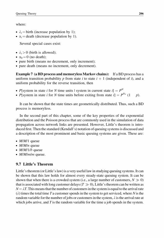
where:
. li¼ birth (increase population by 1);
. ai¼ death (decrease population by 1).
Several special cases exist:
. li> 0 (birth is allowed);
. a0¼ 0 (no death);
. pure birth (means no decrement, only increment);
. pure death (means no increment, only decrement).
Example 7 (a BDprocess andmemorylessMarkov chains): If a BDprocess has a
uniform transition probability p from state i to state i þ 1 (independent of i), and a
uniform probability for the reverse transition, then
. P[system in state i for N time units | system in current state i] ¼ PN
. P[system in state i for N time units before exiting from state i] ¼ PN� (1 p).
It can be shown that the state times are geometrically distributed. Thus, such a BD
process is memoryless.
In the second part of this chapter, some of the key properties of the exponential
distribution and the Poisson process that are commonly used in the simulation of data
propagation across network links are presented. However, Little’s theorem is intro-
duced first. Then the standard (Kendall’s) notation of queuing systems is discussed and
a description of the most prominent and basic queuing systems are given. These are:
. M/M/1 queue
. M/M/n queue
. M/M/1/b queue
. M/M/m/m queue.
9.7 Little’s Theorem
Little’s theorem (or Little’s law) is a very useful law in studying queuing systems. It can
be shown that this law holds for almost every steady-state queuing system. It can be
shown that when there is a crowded system (i.e., a large number of customers, N 0)
that is associatedwith long customer delays (T 0), Little’s theorem can bewritten as
N¼ lT. Thismeans that the number of customers in the system is equal to the arrival rate
(l) times the total time T a customer spends in the system to get serviced, whereN is the
randomvariable for the number of jobs or customers in the system, l is the arrival rate atwhich jobs arrive, and T is the random variable for the time a job spends in the system.
Queuing Theory 206
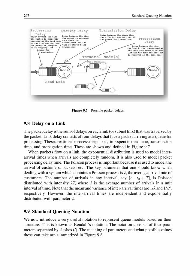
9.8 Delay on a Link
The packet delay is the sumof delays on each link (or subnet link) thatwas traversed by
the packet. Link delay consists of four delays that face a packet arriving at a queue for
processing. These are: time to process the packet, time spent in the queue, transmission
time, and propagation time. These are shown and defined in Figure 9.7.
When packets flow on a link, the exponential distribution is used to model inter-
arrival times when arrivals are completely random. It is also used to model packet
processing delay time. The Poisson process is important because it is used tomodel the
arrival of customers, packets, etc. The key parameter that one should know when
dealing with a systemwhich contains a Poisson process is l, the average arrival rate ofcustomers. The number of arrivals in any interval, say [t0, t0 þ T], is Poisson
distributed with intensity lT, where l is the average number of arrivals in a unit
interval of time. Note that themean and variance of inter-arrival times are 1/l and 1/l2,respectively. However, the inter-arrival times are independent and exponentially
distributed with parameter l.
9.9 Standard Queuing Notation
We now introduce a very useful notation to represent queue models based on their
structure. This is known as Kendall’s notation. The notation consists of four para-
meters separated by slashes (/). The meaning of parameters and what possible values
these can take are summarized in Figure 9.8.
Figure 9.7 Possible packet delays
207 Standard Queuing Notation
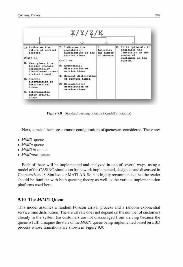
Next, someof themore commonconfigurations of queues are considered. These are:
. M/M/1 queue
. M/M/n queue
. M/M/1/b queue
. M/M/m/m queue.
Each of these will be implemented and analyzed in one of several ways, using a
model of theCASiNO simulation framework implemented, designed, and discussed in
Chapters 6 and 8, SimJava, or MATLAB. So, it is highly recommended that the reader
should be familiar with both queuing theory as well as the various implementation
platforms used here.
9.10 The M/M/1 Queue
This model assumes a random Poisson arrival process and a random exponential
service time distribution. The arrival rate does not depend on the number of customers
already in the system (so customers are not discouraged from arriving because the
queue is full). Imagine the state of theM/M/1 queue being implemented based on a BD
process whose transitions are shown in Figure 9.9.
Figure 9.8 Standard queuing notation (Kendall’s notation)
Queuing Theory 208
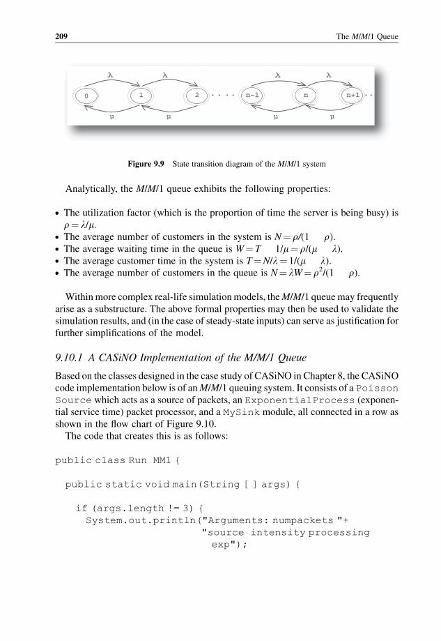
Analytically, the M/M/1 queue exhibits the following properties:
. The utilization factor (which is the proportion of time the server is being busy) is
r¼ l/m.. The average number of customers in the system is N¼ r/(1 r).. The average waiting time in the queue is W¼ T 1/m¼ r/(m l).. The average customer time in the system is T¼N/l¼ 1/(m l).. The average number of customers in the queue is N¼ lW¼ r2/(1 r).
Withinmore complex real-life simulationmodels, theM/M/1 queuemay frequently
arise as a substructure. The above formal properties may then be used to validate the
simulation results, and (in the case of steady-state inputs) can serve as justification for
further simplifications of the model.
9.10.1 A CASiNO Implementation of the M/M/1 Queue
Based on the classes designed in the case study of CASiNO in Chapter 8, the CASiNO
code implementation below is of anM/M/1 queuing system. It consists of a Poisson
Source which acts as a source of packets, an ExponentialProcess (exponen-
tial service time) packet processor, and a MySink module, all connected in a row as
shown in the flow chart of Figure 9.10.
The code that creates this is as follows:
public class Run MM1 {
public static void main(String [ ] args) {
if (args.length != 3) {
System.out.println("Arguments: numpackets "+
"source intensity processing
exp");
0 1 2 n–1. . . . ..n+1n
µ µµµ
Figure 9.9 State transition diagram of the M/M/1 system
209 The M/M/1 Queue
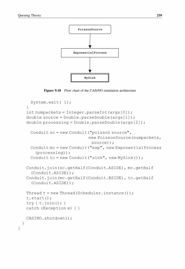
MySink
ExponentialProcess
PoissonSource
Figure 9.10 Flow chart of the CASiNO simulation architecture
System.exit( 1);
}
int numpackets = Integer.parseInt(args[0]);
double source = Double.parseDouble(args[1]);
double processing = Double.parseDouble(args[2]);
Conduit sc = new Conduit("poisson source",
new PoissonSource(numpackets,
source));
Conduit mc = new Conduit("exp", new ExponentialProcess
(processing));
Conduit tc = new Conduit("sink", new MySink());
Conduit.join(sc.getHalf(Conduit.ASIDE), mc.getHalf
(Conduit.ASIDE));
Conduit.join(mc.getHalf(Conduit.BSIDE), tc.getHalf
(Conduit.ASIDE));
Thread t = new Thread(Scheduler.instance());
t.start();
try { t.join(); }
catch (Exception e) { }
CASINO.shutdown();
}
}
Queuing Theory 210
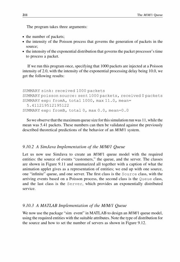
The program takes three arguments:
. the number of packets;
. the intensity of the Poisson process that governs the generation of packets in the
source;. the intensity of the exponential distribution that governs the packet processor’s time
to process a packet.
If we run this program once, specifying that 1000 packets are injected at a Poisson
intensity of 2.0, with the intensity of the exponential processing delay being 10.0, we
get the following results:
SUMMARY sink: received 1000 packets
SUMMARY poisson source: sent 1000 packets, received 0 packets
SUMMARY exp: fromA, total 1000, max 11.0, mean=
5.411219512195122
SUMMARY exp: fromB, total 0, max 0.0, mean=0.0
Sowe observe that themaximumqueue size for this simulation runwas 11,while the
mean was 5.41 packets. These numbers can then be validated against the previously
described theoretical predictions of the behavior of an M/M/1 system.
9.10.2 A SimJava Implementation of the M/M/1 Queue
Let us now use SimJava to create an M/M/1 queue model with the required
entities: the source of events “customers,” the queue, and the server. The classes
are shown in Figure 9.11 and summarized all together with a caption of what the
animation applet gives as a representation of entities; we end up with one source,
one “infinite” queue, and one server. The first class is the Source class, with the
arriving events based on a Poisson process, the second class is the Queue class,
and the last class is the Server, which provides an exponentially distributed
service.
9.10.3 A MATLAB Implementation of the M/M/1 Queue
We now use the package “sim event” in MATLAB to design anM/M/1 queue model,
using the required entities with the suitable attributes. Note the type of distribution for
the source and how to set the number of servers as shown in Figure 9.12.
211 The M/M/1 Queue
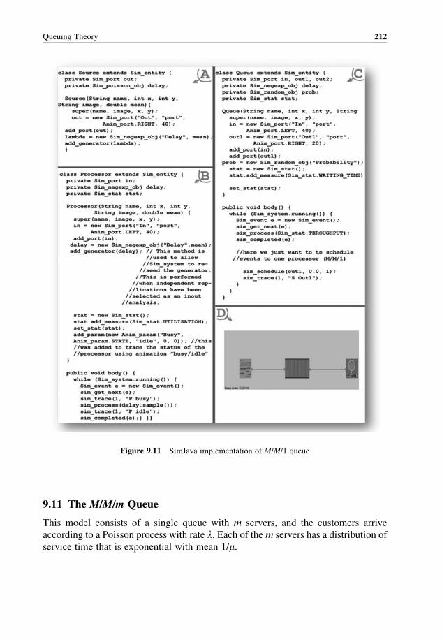
9.11 The M/M/m Queue
This model consists of a single queue with m servers, and the customers arrive
according to a Poisson process with rate l. Each of the m servers has a distribution of
service time that is exponential with mean 1/m.
Figure 9.11 SimJava implementation of M/M/1 queue
Queuing Theory 212

Analytically, the M/M/m queue exhibits the following properties:
. The server utilization is measured by r¼ l/mm, where m is the number of servers.
. The average waiting time in a queue of customers is:
W ¼ NQ
l¼ rpQ
lð1 rÞ :
such that the average number of customers in the queue NQ is:
NQ ¼X¥n 0
npmþ n ¼ rpQ1 r
:
. The average customer time in the system is:
T ¼ 1
mþW ¼ 1
mþ pQ
mm l:
. The average number of customers in the system is:
N ¼ lT ¼ mrþ rpQ1 r
:
Within a more complex real-life simulation model, the M/M/m queue may fre-
quently arise as a substructure. The above formal properties may then be used to
Figure 9.12 A snapshot of MATLAB M/M/1 queue implementation
213 The M/M/m Queue
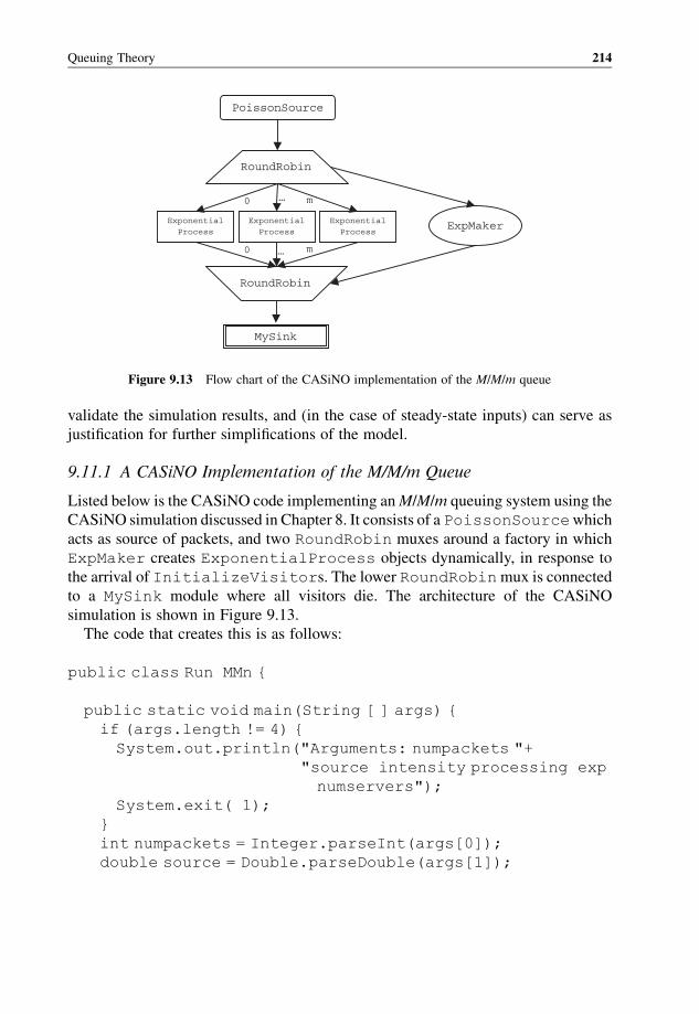
validate the simulation results, and (in the case of steady-state inputs) can serve as
justification for further simplifications of the model.
9.11.1 A CASiNO Implementation of the M/M/m Queue
Listed below is the CASiNO code implementing anM/M/m queuing system using the
CASiNO simulation discussed in Chapter 8. It consists of a PoissonSourcewhich
acts as source of packets, and two RoundRobin muxes around a factory in which
ExpMaker creates ExponentialProcess objects dynamically, in response to
the arrival of InitializeVisitors. The lower RoundRobinmux is connected
to a MySink module where all visitors die. The architecture of the CASiNO
simulation is shown in Figure 9.13.
The code that creates this is as follows:
public class Run MMn {
public static void main(String [ ] args) {
if (args.length != 4) {
System.out.println("Arguments: numpackets "+
"source intensity processing exp
numservers");
System.exit( 1);
}
int numpackets = Integer.parseInt(args[0]);
double source = Double.parseDouble(args[1]);
RoundRobin
RoundRobin
MySink
ExpMakerExponentialProcess
ExponentialProcess
ExponentialProcess
0 … m
0 … m
PoissonSource
Figure 9.13 Flow chart of the CASiNO implementation of the M/M/m queue
Queuing Theory 214
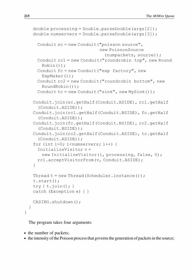
double processing = Double.parseDouble(args[2]);
double numservers = Double.parseDouble(args[3]);
Conduit sc = new Conduit("poisson source",
new PoissonSource
(numpackets, source));
Conduit rc1 = new Conduit("roundrobin top", new Round
Robin());
Conduit fc = new Conduit("exp factory", new
ExpMaker());
Conduit rc2 = new Conduit("roundrobin bottom", new
RoundRobin());
Conduit tc = new Conduit("sink", new MySink());
Conduit.join(sc.getHalf(Conduit.ASIDE), rc1.getHalf
(Conduit.ASIDE));
Conduit.join(rc1.getHalf(Conduit.BSIDE), fc.getHalf
(Conduit.ASIDE));
Conduit.join(fc.getHalf(Conduit.BSIDE), rc2.getHalf
(Conduit.BSIDE));
Conduit.join(rc2.getHalf(Conduit.ASIDE), tc.getHalf
(Conduit.ASIDE));
for (int i=0; i<numservers; i++) {
InitializeVisitor v =
new InitializeVisitor(i, processing, false, 0);
rc1.acceptVisitorFrom(v, Conduit.ASIDE);
}
Thread t = new Thread(Scheduler.instance());
t.start();
try { t.join(); }
catch (Exception e) { }
CASINO.shutdown();
}
}
The program takes four arguments:
. the number of packets;
. the intensity of the Poissonprocess that governs thegenerationofpackets in the source;
215 The M/M/m Queue
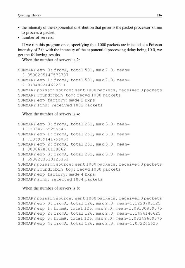
. the intensity of the exponential distribution that governs the packet processor’s time
to process a packet.. number of servers.
If we run this program once, specifying that 1000 packets are injected at a Poisson
intensity of 2.0, with the intensity of the exponential processing delay being 10.0, we
get the following results.
When the number of servers is 2:
SUMMARY exp 0: fromA, total 501, max 7.0, mean=
3.0590295147573787
SUMMARY exp 1: fromA, total 501, max 7.0, mean=
2.978489244622311
SUMMARY poisson source: sent 1000 packets, received 0 packets
SUMMARY roundrobin top: recvd 1000 packets
SUMMARY exp factory: made 2 Exps
SUMMARY sink: received 1002 packets
When the number of servers is 4:
SUMMARY exp 0: fromA, total 251, max 3.0, mean=
1.720347155255545
SUMMARY exp 1: fromA, total 251, max 3.0, mean=
1.7135969141755063
SUMMARY exp 2: fromA, total 251, max 3.0, mean=
1.800867888138862
SUMMARY exp 3: fromA, total 251, max 3.0, mean=
1.6938283510125363
SUMMARY poisson source: sent 1000 packets, received 0 packets
SUMMARY roundrobin top: recvd 1000 packets
SUMMARY exp factory: made 4 Exps
SUMMARY sink: received 1004 packets
When the number of servers is 8:
SUMMARY poisson source: sent 1000 packets, received 0 packets
SUMMARY exp 0: fromA, total 126, max 2.0, mean=1.1220703125
SUMMARY exp 1: fromA, total 126, max 2.0, mean=1.09130859375
SUMMARY exp 2: fromA, total 126, max 2.0, mean=1.1494140625
SUMMARY exp 3: fromA, total 126, max 2.0, mean=1.08349609375
SUMMARY exp 4: fromA, total 126, max 2.0, mean=1.072265625
Queuing Theory 216
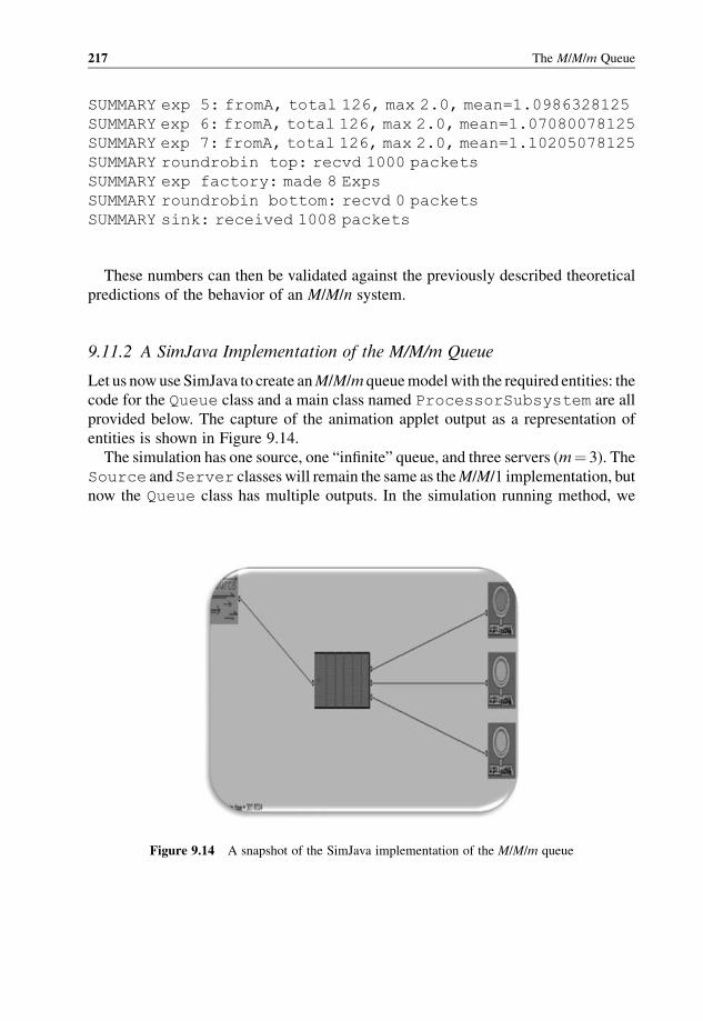
SUMMARY exp 5: fromA, total 126, max 2.0, mean=1.0986328125
SUMMARY exp 6: fromA, total 126, max 2.0, mean=1.07080078125
SUMMARY exp 7: fromA, total 126, max 2.0, mean=1.10205078125
SUMMARY roundrobin top: recvd 1000 packets
SUMMARY exp factory: made 8 Exps
SUMMARY roundrobin bottom: recvd 0 packets
SUMMARY sink: received 1008 packets
These numbers can then be validated against the previously described theoretical
predictions of the behavior of an M/M/n system.
9.11.2 A SimJava Implementation of the M/M/m Queue
Let us nowuse SimJava to create anM/M/m queuemodelwith the required entities: the
code for the Queue class and a main class named ProcessorSubsystem are all
provided below. The capture of the animation applet output as a representation of
entities is shown in Figure 9.14.
The simulation has one source, one “infinite” queue, and three servers (m¼ 3). The
Source andServer classes will remain the same as theM/M/1 implementation, but
now the Queue class has multiple outputs. In the simulation running method, we
Figure 9.14 A snapshot of the SimJava implementation of the M/M/m queue
217 The M/M/m Queue
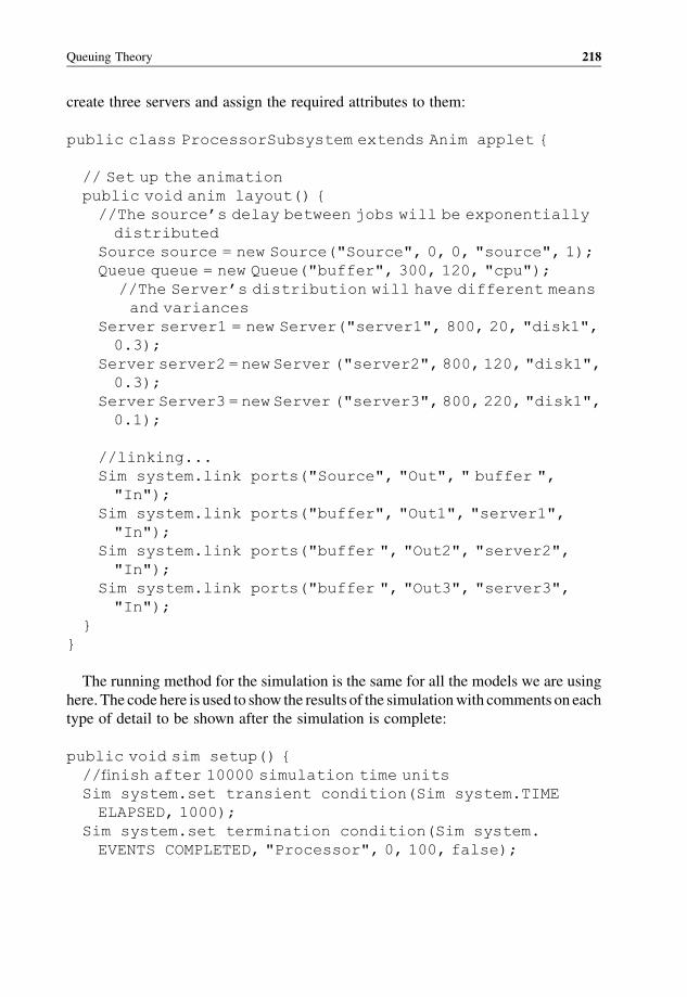
create three servers and assign the required attributes to them:
public class ProcessorSubsystem extends Anim applet {
// Set up the animation
public void anim layout() {
//The source’s delay between jobs will be exponentially
distributed
Source source = new Source("Source", 0, 0, "source", 1);
Queue queue = new Queue("buffer", 300, 120, "cpu");
//The Server’s distribution will have different means
and variances
Server server1 = new Server("server1", 800, 20, "disk1",
0.3);
Server server2 = new Server ("server2", 800, 120, "disk1",
0.3);
Server Server3 = new Server ("server3", 800, 220, "disk1",
0.1);
//linking...
Sim system.link ports("Source", "Out", " buffer ",
"In");
Sim system.link ports("buffer", "Out1", "server1",
"In");
Sim system.link ports("buffer ", "Out2", "server2",
"In");
Sim system.link ports("buffer ", "Out3", "server3",
"In");
}
}
The running method for the simulation is the same for all the models we are using
here. The code here is used to show the results of the simulationwith comments on each
type of detail to be shown after the simulation is complete:
public void sim setup() {
//finish after 10000 simulation time units
Sim system.set transient condition(Sim system.TIME
ELAPSED, 1000);
Sim system.set termination condition(Sim system.
EVENTS COMPLETED, "Processor", 0, 100, false);
Queuing Theory 218
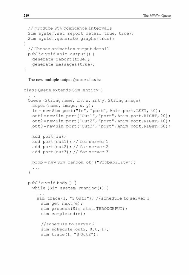
// produce 95% confidence intervals
Sim system.set report detail(true, true);
Sim system.generate graphs(true);
}
// Choose animation output detail
public void anim output() {
generate report(true);
generate messages(true);
}
The new multiple-output Queue class is:
class Queue extends Sim entity {
...
Queue (String name, int x, int y, String image)
super(name, image, x, y);
in = new Sim port("In", "port", Anim port.LEFT, 40);
out1=newSim port("Out1","port",Anim port.RIGHT,20);
out2=newSim port("Out2","port",Anim port.RIGHT,40);
out3=newSim port("Out3","port",Anim port.RIGHT,60);
add port(in);
add port(out1); // for server 1
add port(out2); // for server 2
add port(out3); // for server 3
prob = new Sim random obj("Probability");
...
}
public void body() {
while (Sim system.running()) {
...
sim trace(1, "S Out1"); //schedule to server 1
sim get next(e);
sim process(Sim stat.THROUGHPUT);
sim completed(e);
//schedule to server 2
sim schedule(out2, 0.0, 1);
sim trace(1, "S Out2");
219 The M/M/m Queue
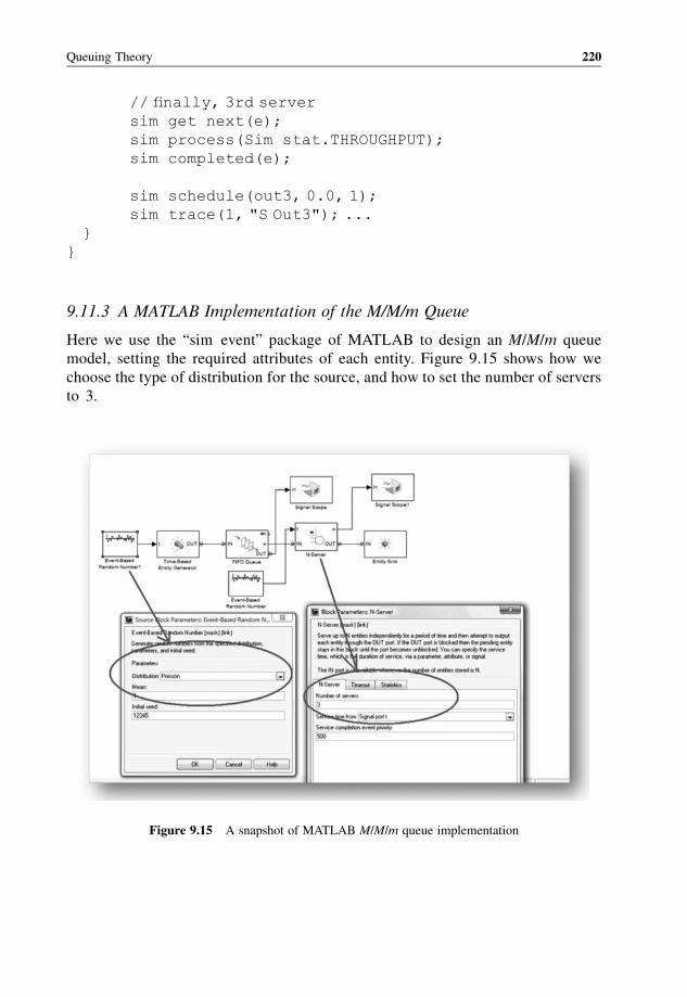
// finally, 3rd server
sim get next(e);
sim process(Sim stat.THROUGHPUT);
sim completed(e);
sim schedule(out3, 0.0, 1);
sim trace(1, "S Out3"); ...
}
}
9.11.3 A MATLAB Implementation of the M/M/m Queue
Here we use the “sim event” package of MATLAB to design an M/M/m queue
model, setting the required attributes of each entity. Figure 9.15 shows how we
choose the type of distribution for the source, and how to set the number of servers
to 3.
Figure 9.15 A snapshot of MATLAB M/M/m queue implementation
Queuing Theory 220
9.12 The M/M/1/b Queue
This queue is a more realistic extension of theM/M/1 queue. It assumes that there is a
limit to the size of queue “or buffer” which makes it possible to refuse receiving any
extra customers when the limit b is exceeded. Arrivals continue to occur according to a
Poisson process, and customer service time is exponentially distributed. There is just
one server used with a finite queue length of size b.
Analytically, the M/M/1/b queue exhibits the following properties:
. The server throughput is:
1 rb
1 rbþ 1l:
. The average number of customers in the system is:
N ¼ r1 r
ðbþ 1Þrbþ 1
1 rbþ 1:
. The average time spent by a customer in the system (queue time þ processing
time) is:
T ¼ average number of customers in system
service throughput:
. The blocking probability (the probability that a customer will face a full queue and
gets rejected) is:
Pb ¼ ð1 rÞrb1 rbþ 1
:
. The average queue length (the number of customers in the queue) is:
LQ ¼ r1 rbþ 1
ð1 rbÞ1 r
brb� �
:
Within a more complex real-life simulation model, the M/M/1/b queue may
frequently arise as a substructure. The above formal properties may then be used to
validate the simulation results, and (in the case of steady-state inputs) can serve as
justification for further simplifications of the model.
221 The M/M/1/b Queue
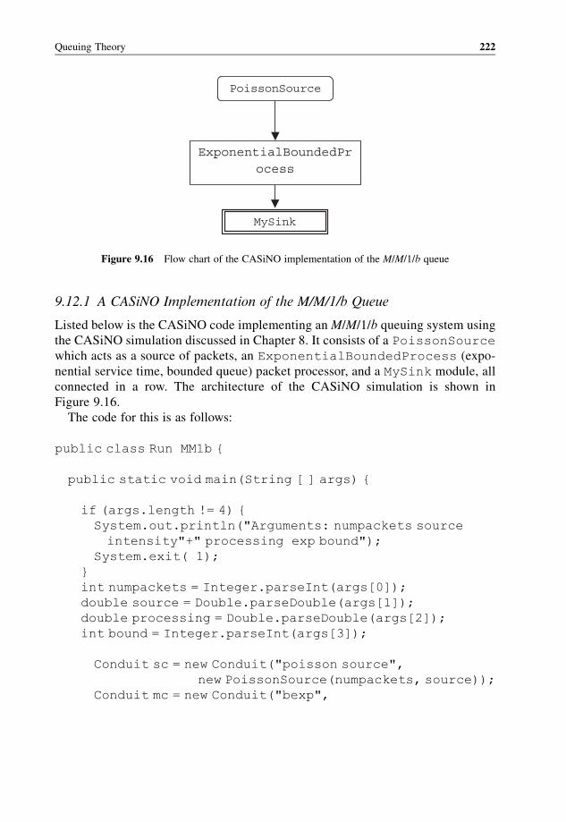
9.12.1 A CASiNO Implementation of the M/M/1/b Queue
Listed below is the CASiNO code implementing an M/M/1/b queuing system using
the CASiNO simulation discussed in Chapter 8. It consists of a PoissonSource
which acts as a source of packets, an ExponentialBoundedProcess (expo-
nential service time, bounded queue) packet processor, and a MySink module, all
connected in a row. The architecture of the CASiNO simulation is shown in
Figure 9.16.
The code for this is as follows:
public class Run MM1b {
public static void main(String [ ] args) {
if (args.length != 4) {
System.out.println("Arguments: numpackets source
intensity"+" processing exp bound");
System.exit( 1);
}
int numpackets = Integer.parseInt(args[0]);
double source = Double.parseDouble(args[1]);
double processing = Double.parseDouble(args[2]);
int bound = Integer.parseInt(args[3]);
Conduit sc = new Conduit("poisson source",
new PoissonSource(numpackets, source));
Conduit mc = new Conduit("bexp",
MySink
ExponentialBoundedProcess
PoissonSource
Figure 9.16 Flow chart of the CASiNO implementation of the M/M/1/b queue
Queuing Theory 222
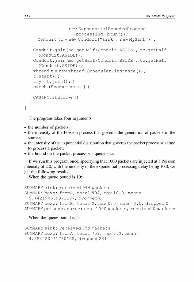
new ExponentialBoundedProcess
(processing, bound));
Conduit tc = new Conduit("sink", new MySink());
Conduit.join(sc.getHalf(Conduit.ASIDE), mc.getHalf
(Conduit.ASIDE));
Conduit.join(mc.getHalf(Conduit.BSIDE), tc.getHalf
(Conduit.ASIDE));
Thread t = new Thread(Scheduler.instance());
t.start();
try { t.join(); }
catch (Exception e) { }
CASINO.shutdown();
}
}
The program takes four arguments:
. the number of packets;
. the intensity of the Poisson process that governs the generation of packets in the
source;. the intensity of the exponential distribution that governs the packet processor’s time
to process a packet;. the bound on the packet processor’s queue size.
If we run this program once, specifying that 1000 packets are injected at a Poisson
intensity of 2.0, with the intensity of the exponential processing delay being 10.0, we
get the following results.
When the queue bound is 10:
SUMMARY sink: received 994 packets
SUMMARY bexp: fromA, total 994, max 10.0, mean=
5.442190669371197, dropped 6
SUMMARY bexp: fromB, total 0, max 0.0, mean=0.0, dropped 0
SUMMARY poisson source: sent 1000 packets, received 0 packets
When the queue bound is 5:
SUMMARY sink: received 759 packets
SUMMARY bexp: fromA, total 759, max 5.0, mean=
4.354450261780105, dropped 241
223 The M/M/1/b Queue
SUMMARY bexp: fromB, total 0, max 0.0, mean=0.0, dropped 0
SUMMARY poisson source: sent 1000 packets, received 0 packets
When the queue bound is 2:
SUMMARY sink: received 340 packets
SUMMARY bexp: fromA, total 340, max 2.0, mean=
1.94634402945818, dropped 660
SUMMARY bexp: fromB, total 0, max 0.0, mean=0.0, dropped 0
SUMMARY poisson source: sent 1000 packets, received 0 packets
These numbers can then be validated against the previously described theoretical
predictions of the behavior of an M/M/1/b system.
9.12.2 A SimJava Implementation of the M/M/1/b Queue
Let us use SimJava now to create anM/M/1/b queue model with the required entities.
The Queue class is the only one provided below because it is the only one that has a
major change. Using a while statement, we can keep polling on the situation of the
queue until, at some time, “maybe” it gets full. In such a case, no further action,
“preemption of events,” is taken:
// This is the body method of the Queue class
public void body() {
// assign a queue length
int b = 10;
while (Sim system.running()) {
//if number of customers do not exceed length b
while (Sim stat.QUEUE LENGTH <= b) {
Sim event e = new Sim event();
// Accept events only from the source entity
sim get next(e);
sim process(Sim stat.THROUGHPUT);
sim completed(e);
//continue to deal with the server
sim schedule(out1, 0.0, 1);
sim trace(1, "S Out1");
//}
Queuing Theory 224
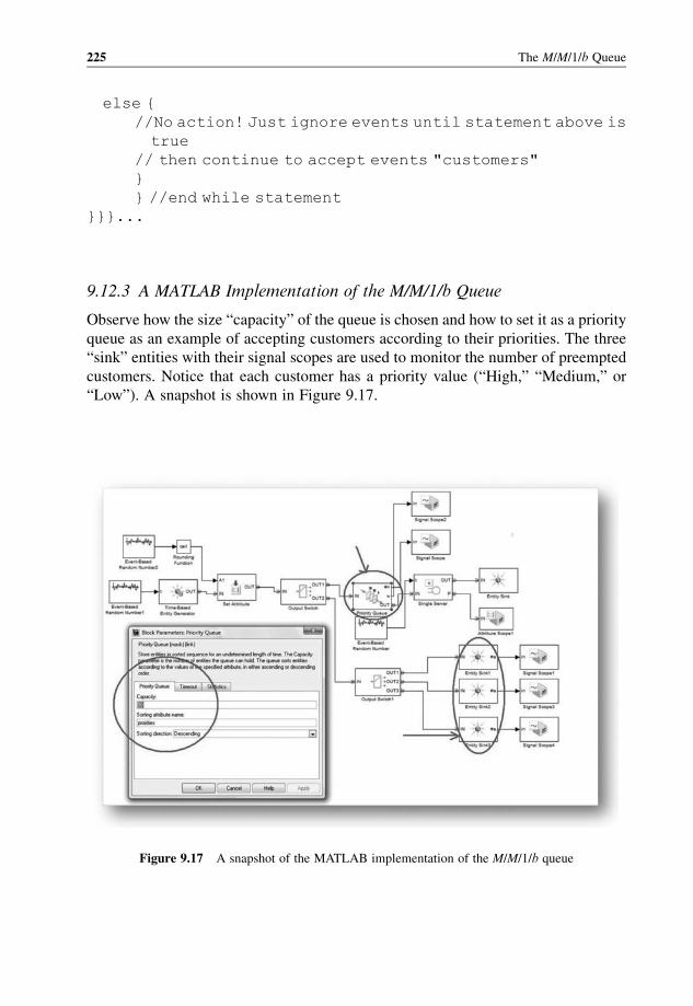
else {
//No action! Just ignore events until statement above is
true
// then continue to accept events "customers"
}
} //end while statement
}}}...
9.12.3 A MATLAB Implementation of the M/M/1/b Queue
Observe how the size “capacity” of the queue is chosen and how to set it as a priority
queue as an example of accepting customers according to their priorities. The three
“sink” entities with their signal scopes are used to monitor the number of preempted
customers. Notice that each customer has a priority value (“High,” “Medium,” or
“Low”). A snapshot is shown in Figure 9.17.
Figure 9.17 A snapshot of the MATLAB implementation of the M/M/1/b queue
225 The M/M/1/b Queue
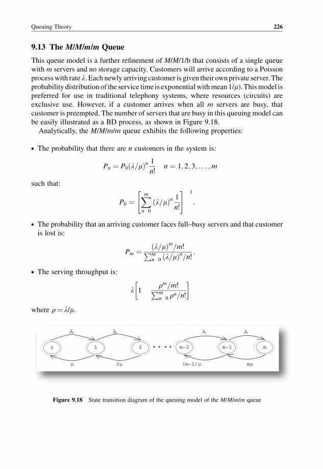
9.13 The M/M/m/m Queue
This queue model is a further refinement of M/M/1/b that consists of a single queue
with m servers and no storage capacity. Customers will arrive according to a Poisson
processwith rate l. Each newly arriving customer is given their ownprivate server. The
probability distribution of the service time is exponentialwithmean1/m). Thismodel is
preferred for use in traditional telephony systems, where resources (circuits) are
exclusive use. However, if a customer arrives when all m servers are busy, that
customer is preempted. The number of servers that are busy in this queuing model can
be easily illustrated as a BD process, as shown in Figure 9.18.
Analytically, the M/M/m/m queue exhibits the following properties:
. The probability that there are n customers in the system is:
Pn ¼ P0ðl=mÞn 1n!
n ¼ 1; 2; 3; . . . ;m
such that:
P0 ¼Xmn 0
ðl=mÞn 1n!
" # 1
:
. The probability that an arriving customer faces full–busy servers and that customer
is lost is:
Pm ¼ ðl=mÞm=m!Pmn 0 ðl=mÞn=n!
:
. The serving throughput is:
l 1rm=m!Pmn 0 rn=n!
� �
where r¼ l/m.
0 1 2 m–2 m–1 m....
(m–1)µ mµ2µµ
Figure 9.18 State transition diagram of the queuing model of the M/M/m/m queue
Queuing Theory 226
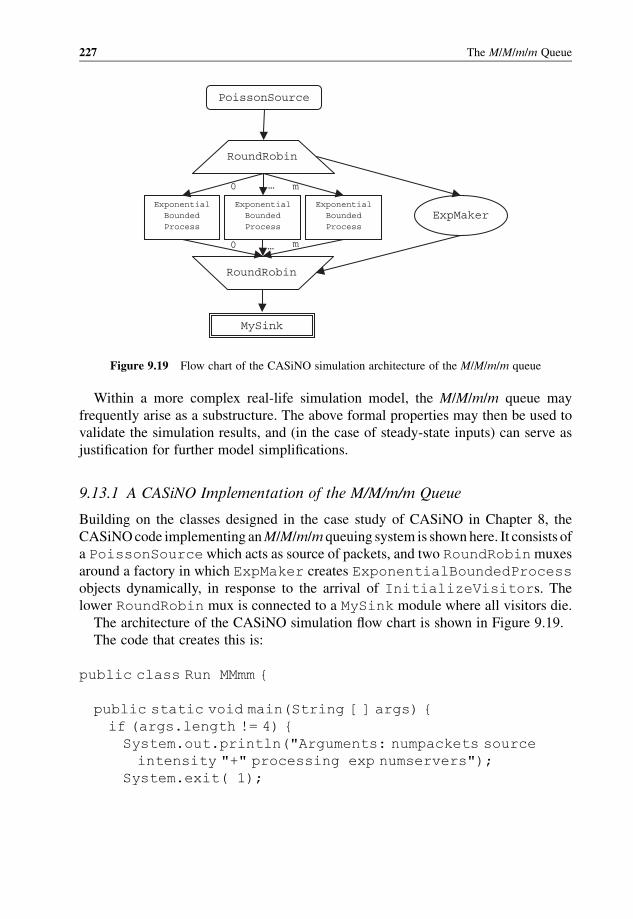
Within a more complex real-life simulation model, the M/M/m/m queue may
frequently arise as a substructure. The above formal properties may then be used to
validate the simulation results, and (in the case of steady-state inputs) can serve as
justification for further model simplifications.
9.13.1 A CASiNO Implementation of the M/M/m/m Queue
Building on the classes designed in the case study of CASiNO in Chapter 8, the
CASiNOcode implementing anM/M/m/m queuing system is shown here. It consists of
a PoissonSourcewhich acts as source of packets, and two RoundRobinmuxes
around a factory in which ExpMaker creates ExponentialBoundedProcess
objects dynamically, in response to the arrival of InitializeVisitors. The
lower RoundRobin mux is connected to a MySink module where all visitors die.
The architecture of the CASiNO simulation flow chart is shown in Figure 9.19.
The code that creates this is:
public class Run MMmm {
public static void main(String [ ] args) {
if (args.length != 4) {
System.out.println("Arguments: numpackets source
intensity "+" processing exp numservers");
System.exit( 1);
RoundRobin
RoundRobin
MySink
ExpMakerExponential
BoundedProcess
ExponentialBoundedProcess
ExponentialBoundedProcess
0 … m
0 … m
PoissonSource
Figure 9.19 Flow chart of the CASiNO simulation architecture of the M/M/m/m queue
227 The M/M/m/m Queue
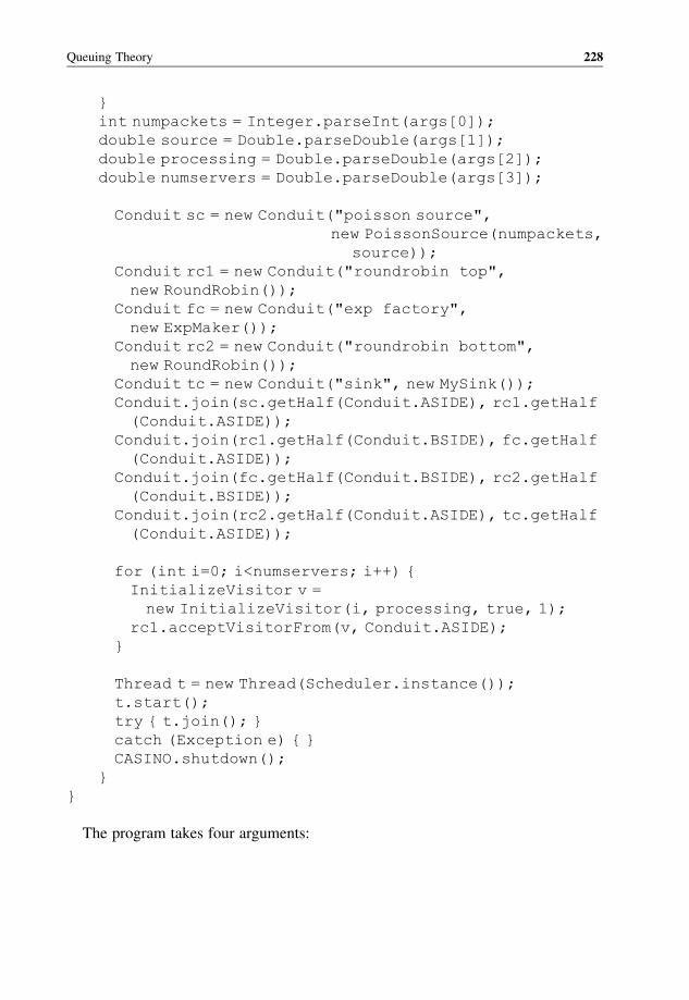
}
int numpackets = Integer.parseInt(args[0]);
double source = Double.parseDouble(args[1]);
double processing = Double.parseDouble(args[2]);
double numservers = Double.parseDouble(args[3]);
Conduit sc = new Conduit("poisson source",
new PoissonSource(numpackets,
source));
Conduit rc1 = new Conduit("roundrobin top",
new RoundRobin());
Conduit fc = new Conduit("exp factory",
new ExpMaker());
Conduit rc2 = new Conduit("roundrobin bottom",
new RoundRobin());
Conduit tc = new Conduit("sink", new MySink());
Conduit.join(sc.getHalf(Conduit.ASIDE), rc1.getHalf
(Conduit.ASIDE));
Conduit.join(rc1.getHalf(Conduit.BSIDE), fc.getHalf
(Conduit.ASIDE));
Conduit.join(fc.getHalf(Conduit.BSIDE), rc2.getHalf
(Conduit.BSIDE));
Conduit.join(rc2.getHalf(Conduit.ASIDE), tc.getHalf
(Conduit.ASIDE));
for (int i=0; i<numservers; i++) {
InitializeVisitor v =
new InitializeVisitor(i, processing, true, 1);
rc1.acceptVisitorFrom(v, Conduit.ASIDE);
}
Thread t = new Thread(Scheduler.instance());
t.start();
try { t.join(); }
catch (Exception e) { }
CASINO.shutdown();
}
}
The program takes four arguments:
Queuing Theory 228
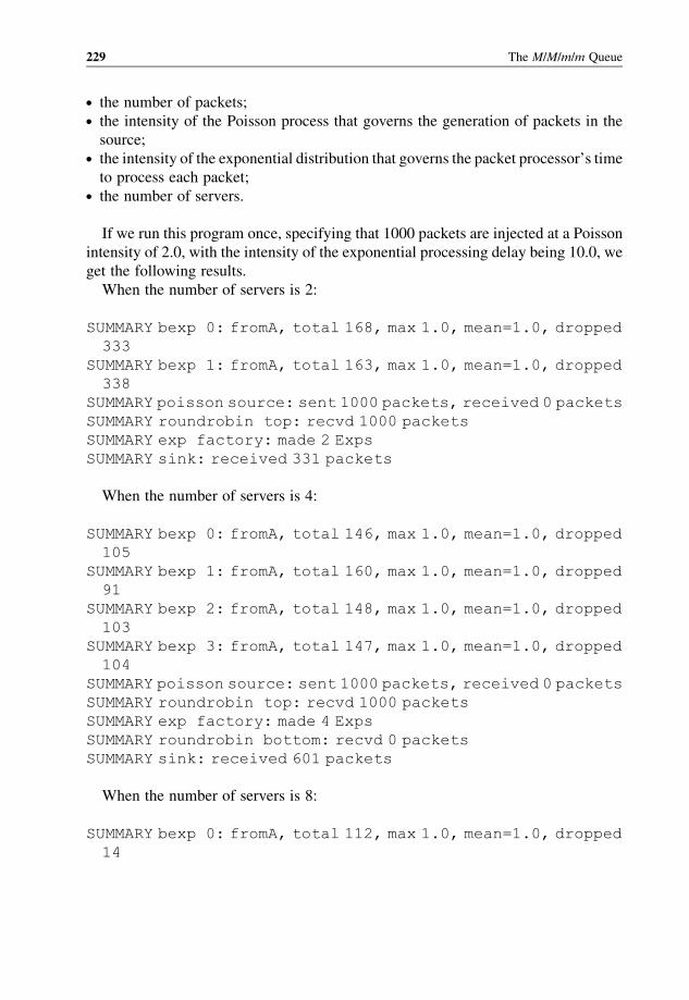
. the number of packets;
. the intensity of the Poisson process that governs the generation of packets in the
source;. the intensity of the exponential distribution that governs the packet processor’s time
to process each packet;. the number of servers.
If we run this program once, specifying that 1000 packets are injected at a Poisson
intensity of 2.0, with the intensity of the exponential processing delay being 10.0, we
get the following results.
When the number of servers is 2:
SUMMARY bexp 0: fromA, total 168, max 1.0, mean=1.0, dropped
333
SUMMARY bexp 1: fromA, total 163, max 1.0, mean=1.0, dropped
338
SUMMARY poisson source: sent 1000 packets, received 0 packets
SUMMARY roundrobin top: recvd 1000 packets
SUMMARY exp factory: made 2 Exps
SUMMARY sink: received 331 packets
When the number of servers is 4:
SUMMARY bexp 0: fromA, total 146, max 1.0, mean=1.0, dropped
105
SUMMARY bexp 1: fromA, total 160, max 1.0, mean=1.0, dropped
91
SUMMARY bexp 2: fromA, total 148, max 1.0, mean=1.0, dropped
103
SUMMARY bexp 3: fromA, total 147, max 1.0, mean=1.0, dropped
104
SUMMARY poisson source: sent 1000 packets, received 0 packets
SUMMARY roundrobin top: recvd 1000 packets
SUMMARY exp factory: made 4 Exps
SUMMARY roundrobin bottom: recvd 0 packets
SUMMARY sink: received 601 packets
When the number of servers is 8:
SUMMARY bexp 0: fromA, total 112, max 1.0, mean=1.0, dropped
14
229 The M/M/m/m Queue
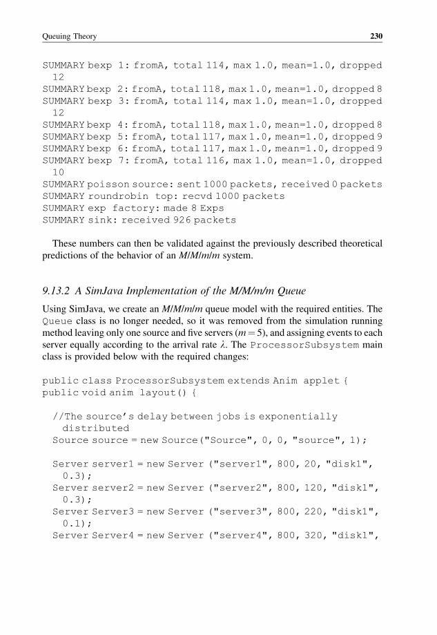
SUMMARY bexp 1: fromA, total 114, max 1.0, mean=1.0, dropped
12
SUMMARY bexp 2: fromA, total 118, max 1.0, mean=1.0, dropped 8
SUMMARY bexp 3: fromA, total 114, max 1.0, mean=1.0, dropped
12
SUMMARY bexp 4: fromA, total 118, max 1.0, mean=1.0, dropped 8
SUMMARY bexp 5: fromA, total 117, max 1.0, mean=1.0, dropped 9
SUMMARY bexp 6: fromA, total 117, max 1.0, mean=1.0, dropped 9
SUMMARY bexp 7: fromA, total 116, max 1.0, mean=1.0, dropped
10
SUMMARY poisson source: sent 1000 packets, received 0 packets
SUMMARY roundrobin top: recvd 1000 packets
SUMMARY exp factory: made 8 Exps
SUMMARY sink: received 926 packets
These numbers can then be validated against the previously described theoretical
predictions of the behavior of an M/M/m/m system.
9.13.2 A SimJava Implementation of the M/M/m/m Queue
Using SimJava, we create an M/M/m/m queue model with the required entities. The
Queue class is no longer needed, so it was removed from the simulation running
method leaving only one source and five servers (m¼ 5), and assigning events to each
server equally according to the arrival rate l. The ProcessorSubsystem main
class is provided below with the required changes:
public class ProcessorSubsystem extends Anim applet {
public void anim layout() {
//The source’s delay between jobs is exponentially
distributed
Source source = new Source("Source", 0, 0, "source", 1);
Server server1 = new Server ("server1", 800, 20, "disk1",
0.3);
Server server2 = new Server ("server2", 800, 120, "disk1",
0.3);
Server Server3 = new Server ("server3", 800, 220, "disk1",
0.1);
Server Server4 = new Server ("server4", 800, 320, "disk1",
Queuing Theory 230
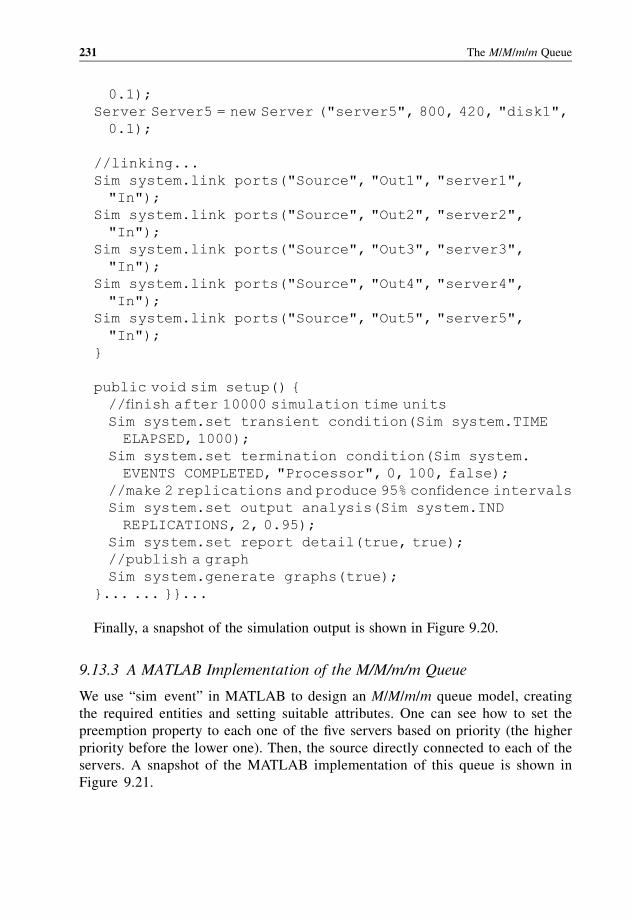
0.1);
Server Server5 = new Server ("server5", 800, 420, "disk1",
0.1);
//linking...
Sim system.link ports("Source", "Out1", "server1",
"In");
Sim system.link ports("Source", "Out2", "server2",
"In");
Sim system.link ports("Source", "Out3", "server3",
"In");
Sim system.link ports("Source", "Out4", "server4",
"In");
Sim system.link ports("Source", "Out5", "server5",
"In");
}
public void sim setup() {
//finish after 10000 simulation time units
Sim system.set transient condition(Sim system.TIME
ELAPSED, 1000);
Sim system.set termination condition(Sim system.
EVENTS COMPLETED, "Processor", 0, 100, false);
//make 2 replications and produce 95% confidence intervals
Sim system.set output analysis(Sim system.IND
REPLICATIONS, 2, 0.95);
Sim system.set report detail(true, true);
//publish a graph
Sim system.generate graphs(true);
}... ... }}...
Finally, a snapshot of the simulation output is shown in Figure 9.20.
9.13.3 A MATLAB Implementation of the M/M/m/m Queue
We use “sim event” in MATLAB to design an M/M/m/m queue model, creating
the required entities and setting suitable attributes. One can see how to set the
preemption property to each one of the five servers based on priority (the higher
priority before the lower one). Then, the source directly connected to each of the
servers. A snapshot of the MATLAB implementation of this queue is shown in
Figure 9.21.
231 The M/M/m/m Queue
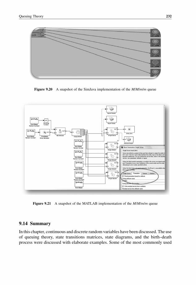
9.14 Summary
In this chapter, continuous and discrete randomvariables have been discussed. The use
of queuing theory, state transitions matrices, state diagrams, and the birth–death
process were discussed with elaborate examples. Some of the most commonly used
Figure 9.21 A snapshot of the MATLAB implementation of the M/M/m/m queue
Figure 9.20 A snapshot of the SimJava implementation of the M/M/m/m queue
Queuing Theory 232

queuing theory techniques have been presented and analyzed. Their corresponding
code using CASiNO, SimJava, and MATLAB simulation techniques has been written
and discussed.
Recommended Reading
[1] L. Kleinrock, Queuing Systems, Volume I: Theory, John Wiley & Sons, Inc., 1975.
[2] A. O. Allen, Probability, Statistics, and Queuing Theory, Academic Press, 1978.
[3] Online: http://en.wikipedia.org/wiki/Chapman Kolmogorov equation
233 Recommended Reading

10
Input Modelingand Output Analysis
Input models greatly influence the outcomes of a simulation model. In real-world
simulation applications, it is crucial that one chooses the appropriate distributions to
represent the input data. If the distribution of inputs is misinterpreted, it will lead to
inaccurate conclusions about the system. This chapter elaborates on the importance of
data collection as a phase within the network modeling project life cycle. It lists the
different data types that need to be collected to support network modeling projects,
how to collect the data, choose the right distribution, and validate the correctness of
one’s choice.
Input models are used to represent the characteristics of randomness or uncertainty
of the input source. Input modeling is the act of choosing the representation that best
expresses the source data. This task often involves choosing an appropriate family of
probability distributions. The task is simplified if one can make any of the following
assumptions:
. The input data can be described as a sequence of independent random variables, and
the distribution for each of them is identical.. The commondistribution sharedby all the randomvariables is one of a general family
of distributions that arewidely implemented inmost simulation systemsor languages,
e.g., the binomial, Poisson, normal, lognormal, exponential, gamma, beta, Erlang,
Weibull, discrete or continuous uniform, triangular, or empirical distributions. The
most commonly used of these are discussed in detail in Chapter 9.. The input data can be represented as being generated by a stationary stochastic
process, for which the probability distribution remains the same for all times. Its
Network Modeling and Simulation M. Guizani, A. Rayes, B. Khan and A. Al Fuqaha
� 2010 John Wiley & Sons, Ltd.
parameters, such as the mean and variance (if they exist), also do not change over
time or position (see Chapter 9 for more details).
There are four major steps for developing a useful model of input data:
1. Collect data from a real-world scenario.
2. Choose a probability distribution to represent the input process.
3. Identify the parameters that are associated with the distribution family.
4. Evaluate the goodness of fit of the chosen distribution and the associated
parameters.
These four steps are the standard procedure to followwhen onewants a close match
between the input model and the true underlying probability distribution associated
with the system. Generally, there are also five basic questions that need to be answered
when there is a given set of data being collected on the element of interest:
. Has the data been collected in an appropriate manner?
. Should a non-parametric model or a parametric probability distribution model be
chosen as the input probabilistic mechanism?. If a parametric model is chosen, what type of distribution will most adequately
describe the data? In other words, what type of random variate generator seems to
generate the same distribution of data?. If a parametric model is chosen, what are the value(s) of parameter(s) that best state
the probability distribution? If the distribution is Gamma(a, b), for instance, then
what is the value of a and b?. After the probability distribution and its associated parameter(s) are chosen, how
much confidence do we have that the chosen values are “best” to describe the input
process?
Detailed discussions of these issues are presented in the following sections.
10.1 Data Collection
Data collection is the most important task when one tries to solve a real physical
problem using a simulation model. Even if a good model structure is chosen, if it is
poorly analyzed or inaccurate data is used, the results generated from the simulation
will be meaningless. There are two approaches that can be elaborated with respect to
the collection of data, the classical approach and the exploratory approach.
In the classical approach, a plan of collecting the data is followed. For instance, if
one wants to study the probability distribution of inter-arrival times between packets
arriving at a server, traffic flow could be recorded on a 24/7 basis in order to come up
Input Modeling and Output Analysis 236
with the data set to analyze. This approach has the advantage that one knows exactly
the data to be modeled. Researchers have proposed [2–5] some suggestions that might
enhance the accuracy of the data being collected:
1. Awell-planned and useful expenditure of time in the initial stages is important. The
input process could have several forms, and it is very likely that the data collection
process is modified several times before the actual data collection, the procedure
becomes well designed. It is also necessary to know how to handle the unusual
circumstances in order to ensure that the appropriate data is available.
2. Try to analyze and collect data simultaneously in order to rule out any data being
collected that is useless to the simulation.
3. Try to associate homogeneous data sets. The quantile–quantile (Q–Q) plot can be
performed for testing the homogeneity between two different data sets. For
example, we might check for homogeneity of data during the same period of time
on a Monday and Tuesday.
4. Try to find out whether there is a relationship between two variables, e.g., by
plotting a scatter diagram to help determine whether two variables are related.
5. Beware that a sequence of independent observations actually may exhibit
autocorrelation.
Some of the pitfalls that could occur during data collections are:
. False aggregation, e.g., model traffic flows per day, but only monthly data is
available.. False classification in time, e.g., data is available for thismonth, but it is necessary to
model the traffic data for next month.. False classification in space, e.g., it is desired to model the traffic flows at the arrival
side, but only departure traffic data is recorded.
10.2 Identifying the Distribution
In this section, we discuss some strategies for selecting families of probability
distributions which can best represent the input process after sample data is collected.
This aspect of the process is more dependent on intuition and experience than it is on
formal theory. For this reason, it is also considered the most difficult part of the overall
process of fitting a distribution to input data. Fortunately, there are some questions that
could help eliminate some probability models:
. What is the source of the data? Is the data finite? Is the data discrete or continuous? Is
the data non-negative? Is it generated by a stationary arrival process?
237 Identifying the Distribution
. Plot a histogram and analyze its shape. This process will rule out several
distributions from further consideration. Does the histogram follow some specific
pattern of the probability distribution? Is it symmetric about the mean? The
different histogramparameters can result inmany different shapes of the histogram
and one may plot several histograms with different parameters in order to acquire
a better accuracy of data distribution to the hypothesis. The histogram can be
constructed as follows:
1. Break up the range of data into equal-width adjacent intervals.
2. Based on the selected intervals, try to appropriately label the horizontal axis.
3. Find out each interval’s frequency of occurrence.
4. Based on the frequencies of each interval, try to appropriately label the vertical
axis.
5. Plot the frequencies on the associated vertical axis.
Select the number of intervals approximately equal to the square root of the
sample size. Thewidth of the intervals should be also chosen properly. If this width is
too wide, the shape of the histogram and details will not give good results. If it is too
narrow, the histogram will be ragged and not smooth. Figure 10.1 presents these
scenarios:
If the data is continuous, the shape of its histogramwill be similar to the probability
density function (PDF) of a theoretical distribution. On the other hand, if the data is
discrete, the histogram associated with it will look like a probability mass function
(PMF) of a theoretical probability distribution.
. Summarize some simple sample statistics in order to help filter the potential choices
of the input data distribution. The following are useful summary statistics:
(a) Minimum X1 and maximum Xn values of data: They are rough estimates of the
range.
(b) Mean m: This is the measure of central tendency, and the sample estimate is
defined by:
X ¼Pn
i 1 Xi
n:
(c) Median x0:5: This is an alternative measure of the central tendency, and the
sample estimate is defined by:
x0:5 ¼Xðnþ 1Þ=2 if n is odd
½Xðn=2Þðn=2Þ þXðn=2Þþ 1�2
if n is even:
8<:
Input Modeling and Output Analysis 238
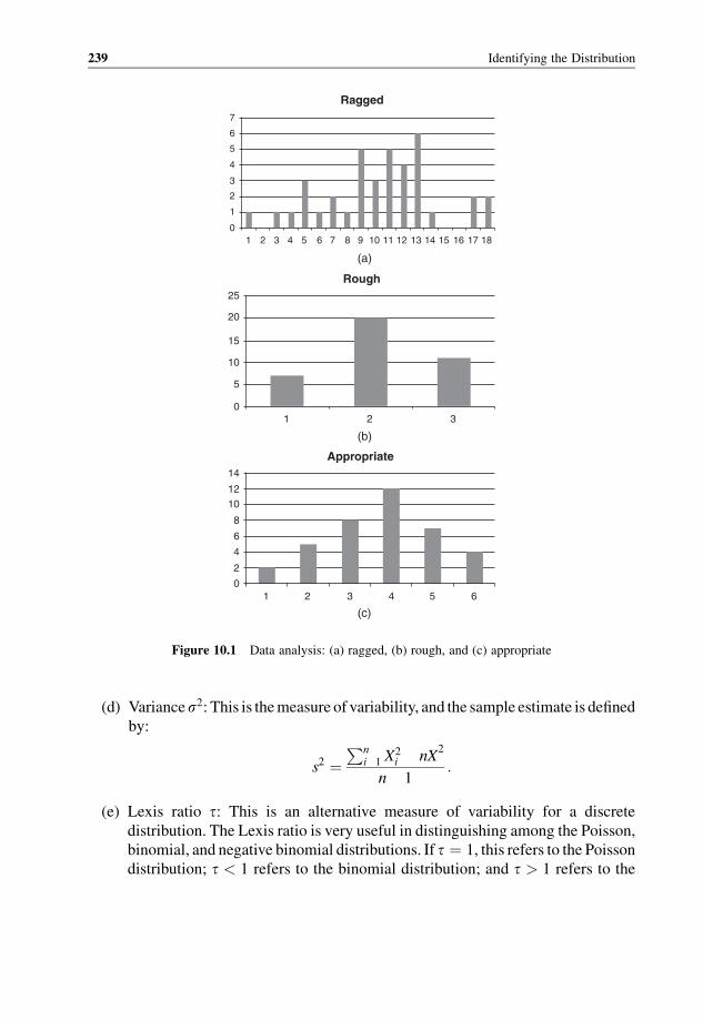
(d) Variances2: This is themeasure of variability, and the sample estimate is defined
by:
s2 ¼Pn
i 1 X2i nX
2
n 1:
(e) Lexis ratio t: This is an alternative measure of variability for a discrete
distribution. The Lexis ratio is very useful in distinguishing among the Poisson,
binomial, and negative binomial distributions. If t ¼ 1, this refers to the Poisson
distribution; t < 1 refers to the binomial distribution; and t > 1 refers to the
25
Rough
20
15
10
14
Appropriate
12
10
8
6
4
2
01 2 3 4 5 6
5
01 2
(b)
(c)
3
7
6
5
4
3
2
1
01 2 3 4 5 6 7 8 9 10 11 12 13 14 15 16 17 18
(a)
Ragged
Figure 10.1 Data analysis: (a) ragged, (b) rough, and (c) appropriate
239 Identifying the Distribution

negative binomial distribution. The Lexis ratio statistic is given by:
t ¼ S2
X:
(f) Coefficient of variation cv ¼ s2p
=m: This is an alternative measure of vari-
ability which can provide useful information on the form of a continuous
distribution. For example, if thevalue of the coefficient of variation is close to 1,
it suggests that the underlying probability distribution is exponential. The
sample estimate cv is defined by:
^cv ¼ S2p
X:
(g) Skewness v ¼ E½ðX mÞ3�=ðs2Þ3=2: This is a measure of symmetry. For in-
stance, the potential input mode would be the normal or uniform distribution if
the sample skewness is close to 0, and the sample estimate is defined by:
v ¼Pn
i 1 ½Xi X�3=nðS2Þ3=2
:
10.3 Estimation of Parameters for Univariate Distributions
After one ormore suitable families of distributions have been selected or hypothesized
during the process as discussed in the previous section, one has to specify the value of
their associated parameters in order to have a completely appropriate distribution
specified for the input process. The i.i.d. data that has just been collectedwill be used to
help choose the distribution which might be the best representation of the input
process. In addition, the same data could be used to help estimate the parameters of the
chosen distribution.
Calculation of themean and variance of the collected data is a good estimation of the
parameters of the distribution (the techniques for the computation of the mean and
variance of the sample data were given in Section 7.1), if the sample raw data is either
discrete or continuous. However, there is a situation that wemight encounter where the
sample data is discrete and has been grouped in a frequency distribution. Then the
sample mean can be calculated as:
X ¼Pk
j 1 fjXj
n
Input Modeling and Output Analysis 240
and the sample variance as:
S2 ¼Pk
j 1 fjX2j nX
2
n 1
where k is the number of values of X and fj is the frequency of Xj of X.
If the data is discrete or continuous and has been put into class intervals, then it is
impossible to obtain the exact sample mean and variance. In this case, one can
calculate the approximate value of the sample mean by:
X¼:Pc
j 1 fjmj
n
and the sample variance is:
S2 ¼:Pc
j 1 fjm2j nX
2
n 1
where fj is the observed frequency in the jth class interval,mj is denoted as themidpoint
of the jth interval, and c is the number of class intervals.
There are two approaches for estimating the parameters of the distribution from the
sample data: themethod ofmoments; andmaximum likelihood estimation techniques.
Both of them produce similar or identical results for many distribution estimations.
The general setting for those techniques are the set of i.i.d. data denoted by
X1;X2; . . . ;Xn and one or more potential distributions that were chosen. Let q denote
the number of unknown parameters (e.g., Uniform(a, b) model, q¼ 2).
The method of moments is an algebraic method for estimating the population
parameters by equating the first q population moments to the first q sample moments
given by:
EðXkÞ ¼ 1
n
Xni 1
xki :
For k¼ 1, 2, . . ., q, and to solve the q� q set of equations for the unknown
parameters q, whereEðXÞ is the expectation of a randomvariableX, or the firstmoment
of the random variable, its variance, s2 or VðXÞ, can also be defined by:
s2 ¼ EðX2Þ ½EðXÞ�2:
For instance, suppose we want to estimate the parameters m and s2ðq ¼ 2Þ for anormal distribution; thenwe have to equate the first two populationmoments to the fist
241 Estimation of Parameters for Univariate Distributions
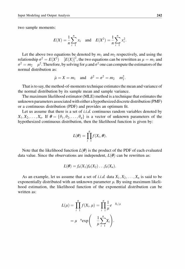
two sample moments:
EðXÞ ¼ 1
n
Xni 1
xi and EðX2Þ ¼ 1
n
Xni 1
x2i :
Let the above two equations be denoted by m1 and m2 respectively, and using the
relationship s2 ¼ EðX2Þ ½EðXÞ�2, the two equations can be rewritten as m ¼ m1 and
s2 ¼ m2 m2. Therefore, by solving form ands2 one can compute the estimators of the
normal distribution as:
m ¼ X ¼ m1 and s2 ¼ s2 ¼ m2 m21:
That is to say, themethod-of-moments technique estimates themean and variance of
the normal distribution by its sample mean and sample variance.
The maximum likelihood estimator (MLE) method is a technique that estimates the
unknownparameters associatedwith either a hypothesized discrete distribution (PMF)
or a continuous distribution (PDF) and provides an optimum fit.
Let us assume that there is a set of i.i.d. continuous random variables denoted by
X1;X2; . . . ;Xn. If h ¼ fy1; y2; . . . ; yqg is a vector of unknown parameters of the
hypothesized continuous distribution, then the likelihood function is given by:
LðhÞ ¼Yni 1
f ðXi; hÞ:
Note that the likelihood function LðhÞ is the product of the PDF of each evaluated
data value. Since the observations are independent, LðhÞ can be rewritten as:
LðhÞ ¼ fyðX1ÞfyðX2Þ . . . fyðXnÞ:
As an example, let us assume that a set of i.i.d. data X1;X2; . . . ;Xn is said to be
exponentially distributed with an unknown parameter m. By using maximum likeli-
hood estimation, the likelihood function of the exponential distribution can be
written as:
LðmÞ ¼Yni 1
f ðXi; mÞ ¼Yni 1
1
me Xi=m
¼ m nexp1
m
Xni 1
Xi
!:
Input Modeling and Output Analysis 242

To find the value of m that maximizes LðmÞ, one can use the log-likelihood functiondefined as:
ln LðmÞ ¼ n lnm1
m
Xni 1
Xi:
In order to maximize the log-likelihood function, standard differential calculus can
be used with respect to m to obtain:
@ ln LðmÞ@m
¼ n
mþ 1
m2Xni 1
Xi:
Equating to zero and solving for m, we can obtain themaximum likelihood estimator
as:
m ¼ 1
n
Xni 1
Xi:
That is, the sample mean X of the data. It is clear that the method of moments and
maximum likelihood estimator generate identical results.
Now we use the same approach to estimate the parameters of discrete distributions
using likelihood function LðhÞ as:
LðhÞ ¼Yni 1
pðXi; hÞ ¼ pyðX1ÞpyðX2Þ . . . pyðXnÞ
where pyðxÞ is the PMF for the chosen distribution with unknown parameter y.For instance, we assume that there is a given data set X1;X2; . . . ;Xn that is
geometrically distributed and pðxÞ ¼ pð1 pÞx for x ¼ 0; 1; . . .. Then, the likelihoodfunction of the geometric distribution is:
LðpÞ ¼ pnð1 pÞPn
i 1Xi :
By taking logarithms, we obtain:
ln LðpÞ ¼ n ln pþXni 1
Xi ln ð1 pÞ:
Then, differentiating LðpÞ we get:
@ ln LðpÞ@p
¼ n
p
Pni 1 Xi
1 p:
243 Estimation of Parameters for Univariate Distributions
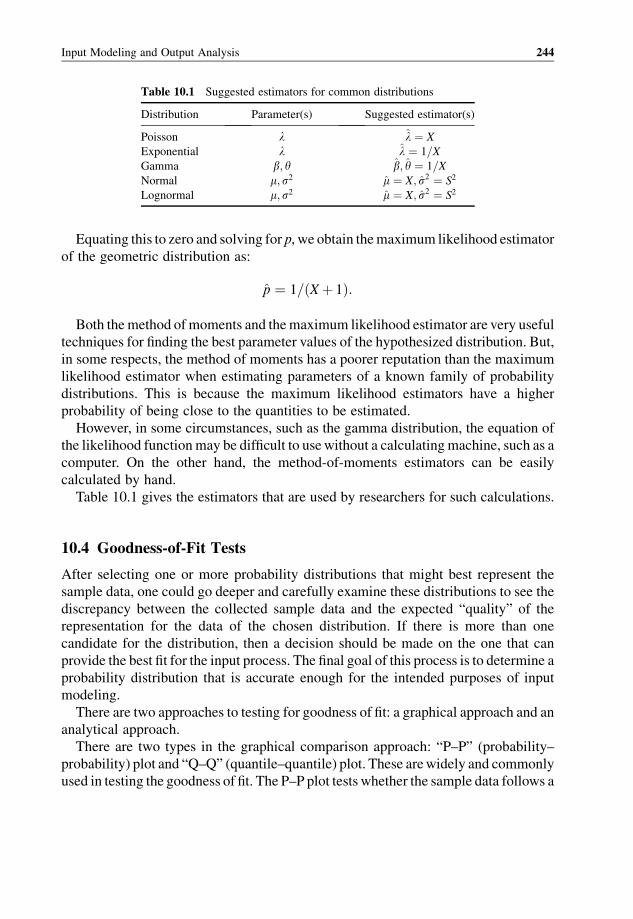
Equating this to zero and solving for p, we obtain themaximum likelihood estimator
of the geometric distribution as:
p ¼ 1=ðXþ 1Þ:
Both themethod of moments and themaximum likelihood estimator are very useful
techniques for finding the best parameter values of the hypothesized distribution. But,
in some respects, the method of moments has a poorer reputation than the maximum
likelihood estimator when estimating parameters of a known family of probability
distributions. This is because the maximum likelihood estimators have a higher
probability of being close to the quantities to be estimated.
However, in some circumstances, such as the gamma distribution, the equation of
the likelihood function may be difficult to usewithout a calculatingmachine, such as a
computer. On the other hand, the method-of-moments estimators can be easily
calculated by hand.
Table 10.1 gives the estimators that are used by researchers for such calculations.
10.4 Goodness-of-Fit Tests
After selecting one or more probability distributions that might best represent the
sample data, one could go deeper and carefully examine these distributions to see the
discrepancy between the collected sample data and the expected “quality” of the
representation for the data of the chosen distribution. If there is more than one
candidate for the distribution, then a decision should be made on the one that can
provide the best fit for the input process. The final goal of this process is to determine a
probability distribution that is accurate enough for the intended purposes of input
modeling.
There are two approaches to testing for goodness of fit: a graphical approach and an
analytical approach.
There are two types in the graphical comparison approach: “P–P” (probability–
probability) plot and “Q–Q” (quantile–quantile) plot. These arewidely and commonly
used in testing the goodness of fit. The P–P plot tests whether the sample data follows a
Table 10.1 Suggested estimators for common distributions
Distribution Parameter(s) Suggested estimator(s)
Poisson l l ¼ X
Exponential l l ¼ 1=XGamma b; y b; y ¼ 1=XNormal m; s2 m ¼ X; s2 ¼ S2
Lognormal m; s2 m ¼ X; s2 ¼ S2
Input Modeling and Output Analysis 244
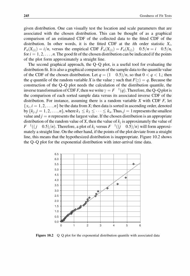
given distribution. One can visually test the location and scale parameters that are
associated with the chosen distribution. This can be thought of as a graphical
comparison of an estimated CDF of the collected data to the fitted CDF of the
distribution. In other words, it is the fitted CDF at the ith order statistic Xi,
FnðXðiÞÞ ¼ i=n, versus the empirical CDF ~FnðXðiÞÞ ¼ FnðXðiÞÞ 0:5=n ¼ i 0:5=n,for i ¼ 1; 2; . . . ; n. The good fit of the chosen distribution can be indicated if the pointsof the plot form approximately a straight line.
The second graphical approach, the Q–Q plot, is a useful tool for evaluating the
distribution fit. It is also a graphical comparison of the sample data to the quantile value
of the CDF of the chosen distribution. Let q ¼ ð1 0:5Þ=n, so that 0 < q < 1,; then
the q quantile of the random variable X is the value g such that FðgÞ ¼ q. Because the
construction of the Q–Q plot needs the calculation of the distribution quantile, the
inverse transformation ofCDFF, thenwewrite g ¼ F 1ðqÞ. Therefore, theQ–Qplot is
the comparison of each sorted sample data versus its associated inverse CDF of the
distribution. For instance, assuming there is a random variable X with CDF F, let
fxi; i ¼ 1; 2; . . . ; ng be the data from X; then data is sorted in ascending order, denoted
byfkj; j ¼ 1; 2; . . . ; ng,wherek1 � k2 � � � � � kn. Thus, j ¼ 1 represents the smallest
value and j ¼ n represents the largest value. If the chosen distribution is an appropriate
distribution of the random value of X, then the value of kj is approximately the value of
F 1ðð j 0:5Þ=nÞ. Therefore, a plot of kj versus F 1ððj 0:5Þ=nÞ will form approxi-
mately a straight line. On the other hand, if the points of the plot deviate from a straight
line, this means that the hypothesized distribution is inappropriate. Figure 10.2 shows
the Q–Q plot for the exponential distribution with inter-arrival time data.
6.5
6.0
5.5
5.0
4.5
4.0
3.5
3.0
2.5
2.0
1.5
1.0
0.5
0.00 1 2 3 4 5 6
Figure 10.2 Q Q plot for the exponential distribution quantile with associated data
245 Goodness of Fit Tests

Note that both P–P and Q–Q plots are subjective because different experts
would have different visual preferences. One could consider Figure 10.2 as an
example, while others might feel that it is nothing but a straight line. Thus, more
objective techniques have to be adopted. These are the so-called analytical approach
techniques.
In the analytical approach, there are two standard statistical techniques that can be
used: the Kolmogorov–Smirnov test and the chi-square test.
10.4.1 Chi-Square Goodness-of-Fit Test
The chi-square ðw2Þ test is a technique that tests for a null hypothesis that the
distribution of a certain observed event’s frequency in a sample is consistent with
the hypothesized discrete or continuous distribution. In addition, the size of the
sample data must be large enough to make the chi-square goodness-of-fit test more
accurate when the associated parameters are estimated by maximum likelihood
estimators.
The first step in the chi-square test is to arrange the number of observations n into a
set of k cells (class intervals), and then calculate the chi-square statistic by finding the
difference between each observed and expected frequency. The statistical formula of
the chi-square test is given by:
w20 ¼Xki 1
ðOi EiÞ2Ei
whereOi is the observed frequency in the ith cell andEi is the expected frequency in the
same cell, which is asserted by the null hypothesis, and the expected frequency can be
computed by npi, where pi is the hypothesized probability of the ith cell.
Another element of the chi-square test is the degrees of freedom. These can be
computed using k s 1, where s denotes the number of parameters associated
with the hypothesized distribution. The hypotheses of the chi-square test are either
true or false, depending on its critical value with a certain value of level of
significance x2a;k s 1. The null hypothesis will be rejected if w20 is bigger than the
critical value.
When applying the chi-square goodness-of-fit test, the most difficult problems that
one might encounter are choosing the number of cells and finding the minimum value
of the expected frequency. In fact, there is no good definition that can generate and
guarantee good results. Fortunately, there are a few guidelines that can be followed to
achieve this.
First, let us consider the continuous distribution scenario. If the distribution being
tested is continuous, then a technique called the equiprobable approach can be used to
Input Modeling and Output Analysis 246
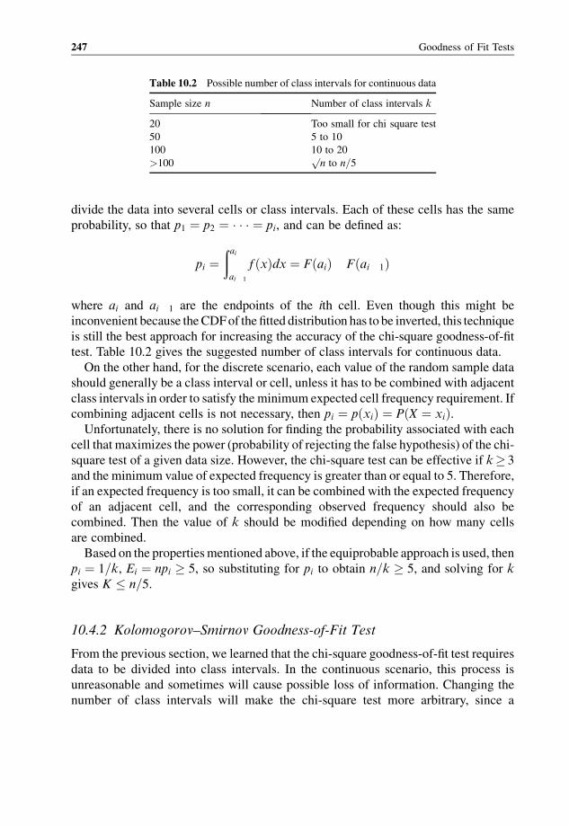
divide the data into several cells or class intervals. Each of these cells has the same
probability, so that p1 ¼ p2 ¼ � � � ¼ pi, and can be defined as:
pi ¼ðaiai 1
f ðxÞdx ¼ FðaiÞ Fðai 1Þ
where ai and ai 1 are the endpoints of the ith cell. Even though this might be
inconvenient because theCDFof the fitted distribution has to be inverted, this technique
is still the best approach for increasing the accuracy of the chi-square goodness-of-fit
test. Table 10.2 gives the suggested number of class intervals for continuous data.
On the other hand, for the discrete scenario, each value of the random sample data
should generally be a class interval or cell, unless it has to be combined with adjacent
class intervals in order to satisfy the minimum expected cell frequency requirement. If
combining adjacent cells is not necessary, then pi ¼ pðxiÞ ¼ PðX ¼ xiÞ.Unfortunately, there is no solution for finding the probability associated with each
cell that maximizes the power (probability of rejecting the false hypothesis) of the chi-
square test of a given data size. However, the chi-square test can be effective if k� 3
and the minimum value of expected frequency is greater than or equal to 5. Therefore,
if an expected frequency is too small, it can be combined with the expected frequency
of an adjacent cell, and the corresponding observed frequency should also be
combined. Then the value of k should be modified depending on how many cells
are combined.
Based on the propertiesmentioned above, if the equiprobable approach is used, then
pi ¼ 1=k, Ei ¼ npi � 5, so substituting for pi to obtain n=k � 5, and solving for k
gives K � n=5.
10.4.2 Kolomogorov–Smirnov Goodness-of-Fit Test
From the previous section, we learned that the chi-square goodness-of-fit test requires
data to be divided into class intervals. In the continuous scenario, this process is
unreasonable and sometimes will cause possible loss of information. Changing the
number of class intervals will make the chi-square test more arbitrary, since a
Table 10.2 Possible number of class intervals for continuous data
Sample size n Number of class intervals k
20 Too small for chi square test
50 5 to 10
100 10 to 20
>100 np
to n=5
247 Goodness of Fit Tests
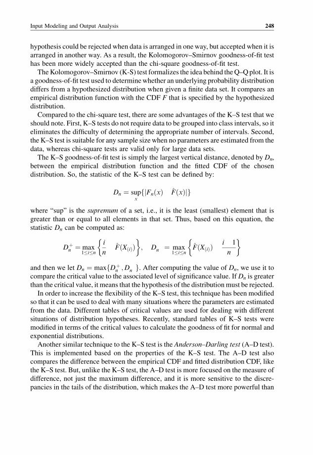
hypothesis could be rejected when data is arranged in oneway, but accepted when it is
arranged in another way. As a result, the Kolomogorov–Smirnov goodness-of-fit test
has been more widely accepted than the chi-square goodness-of-fit test.
TheKolomogorov–Smirnov (K-S) test formalizes the idea behind theQ–Qplot. It is
a goodness-of-fit test used to determinewhether an underlying probability distribution
differs from a hypothesized distribution when given a finite data set. It compares an
empirical distribution function with the CDF F that is specified by the hypothesized
distribution.
Compared to the chi-square test, there are some advantages of the K–S test that we
should note. First, K–S tests do not require data to be grouped into class intervals, so it
eliminates the difficulty of determining the appropriate number of intervals. Second,
the K–S test is suitable for any sample sizewhen no parameters are estimated from the
data, whereas chi-square tests are valid only for large data sets.
The K–S goodness-of-fit test is simply the largest vertical distance, denoted by Dn,
between the empirical distribution function and the fitted CDF of the chosen
distribution. So, the statistic of the K–S test can be defined by:
Dn ¼ supxfjFnðxÞ FðxÞjg
where “sup” is the supremum of a set, i.e., it is the least (smallest) element that is
greater than or equal to all elements in that set. Thus, based on this equation, the
statistic Dn can be computed as:
Dþn ¼ max
1�i�n
i
nFðXðiÞÞ
� �; Dn ¼ max
1�i�nFðXðiÞÞ i 1
n
� �
and then we let Dn ¼ maxfDþn ;Dn g. After computing the value of Dn, we use it to
compare the critical value to the associated level of significance value. IfDn is greater
than the critical value, it means that the hypothesis of the distributionmust be rejected.
In order to increase the flexibility of the K–S test, this technique has been modified
so that it can be used to deal with many situations where the parameters are estimated
from the data. Different tables of critical values are used for dealing with different
situations of distribution hypotheses. Recently, standard tables of K–S tests were
modified in terms of the critical values to calculate the goodness of fit for normal and
exponential distributions.
Another similar technique to the K–S test is the Anderson–Darling test (A–D test).
This is implemented based on the properties of the K–S test. The A–D test also
compares the difference between the empirical CDF and fitted distribution CDF, like
the K–S test. But, unlike the K–S test, the A–D test is more focused on the measure of
difference, not just the maximum difference, and it is more sensitive to the discre-
pancies in the tails of the distribution, which makes the A–D test more powerful than
Input Modeling and Output Analysis 248
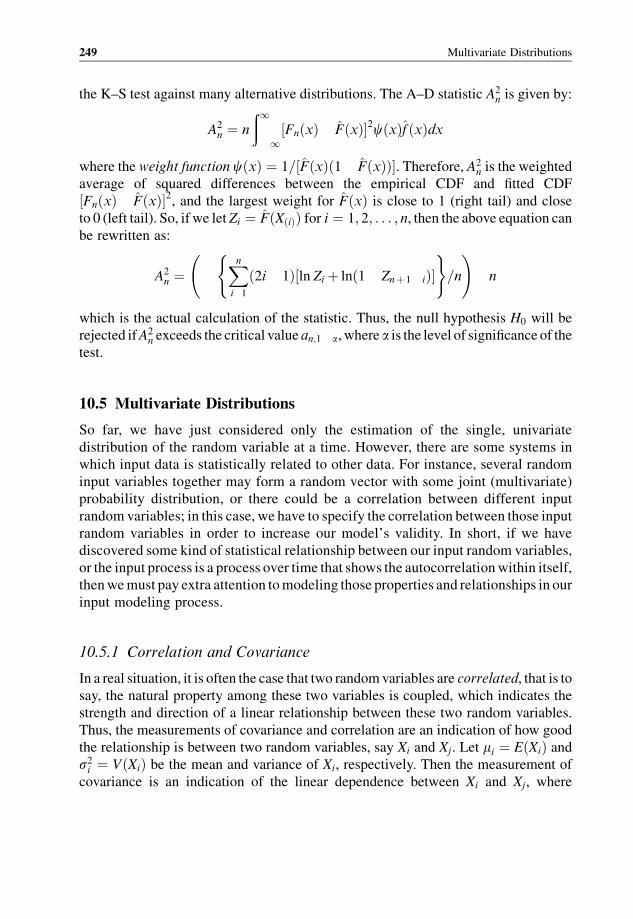
the K–S test against many alternative distributions. The A–D statistic A2n is given by:
A2n ¼ n
ð11½FnðxÞ FðxÞ�2cðxÞf ðxÞdx
where the weight function cðxÞ ¼ 1=½FðxÞð1 FðxÞÞ�. Therefore, A2n is the weighted
average of squared differences between the empirical CDF and fitted CDF
½FnðxÞ FðxÞ�2, and the largest weight for FðxÞ is close to 1 (right tail) and close
to 0 (left tail). So, if we let Zi ¼ FðXðiÞÞ for i ¼ 1; 2; . . . ; n, then the above equation canbe rewritten as:
A2n ¼
Xni 1
ð2i 1Þ½ln Zi þ lnð1 Znþ 1 iÞ�( )
=n
!n
which is the actual calculation of the statistic. Thus, the null hypothesis H0 will be
rejected ifA2n exceeds the critical value an;1 a, where a is the level of significance of the
test.
10.5 Multivariate Distributions
So far, we have just considered only the estimation of the single, univariate
distribution of the random variable at a time. However, there are some systems in
which input data is statistically related to other data. For instance, several random
input variables together may form a random vector with some joint (multivariate)
probability distribution, or there could be a correlation between different input
random variables; in this case, we have to specify the correlation between those input
random variables in order to increase our model’s validity. In short, if we have
discovered some kind of statistical relationship between our input random variables,
or the input process is a process over time that shows the autocorrelationwithin itself,
thenwemust pay extra attention tomodeling those properties and relationships in our
input modeling process.
10.5.1 Correlation and Covariance
In a real situation, it is often the case that two randomvariables are correlated, that is to
say, the natural property among these two variables is coupled, which indicates the
strength and direction of a linear relationship between these two random variables.
Thus, the measurements of covariance and correlation are an indication of how good
the relationship is between two random variables, say Xi and Xj. Let mi ¼ EðXiÞ ands2i ¼ VðXiÞ be the mean and variance of Xi, respectively. Then the measurement of
covariance is an indication of the linear dependence between Xi and Xj, where
249 Multivariate Distributions
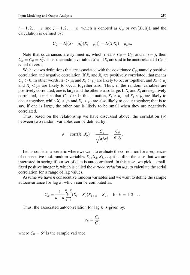
i ¼ 1; 2; . . . ; n and j ¼ 1; 2; . . . ; n, which is denoted as Cij or covðXi;XjÞ, and the
calculation is defined by:
Cij ¼ E½ðXi miÞðXj mjÞ� ¼ EðXiXjÞ mimj:
Note that covariances are symmetric, which means Cij ¼ Cji, and if i ¼ j, then
Cij ¼ Cii ¼ s2i . Thus, the randomvariablesXi andXj are said to be uncorrelated ifCij is
equal to zero.
We have two definitions that are associated with the covarianceCij, namely positive
correlation and negative correlation. If Xi and Xj are positively correlated, that means
Cij > 0, in other words, Xi > mi and Xj > mj are likely to occur together, and Xi < miand Xj < mj are likely to occur together also. Thus, if the random variables are
positively correlated, one is large and the other is also large. If Xi and Xj are negatively
correlated, it means that Cij < 0. In this situation, Xi > mi and Xj < mj are likely to
occur together, while Xi < mi and Xj > mj are also likely to occur together; that is to
say, if one is large, the other one is likely to be small when they are negatively
correlated.
Thus, based on the relationship we have discussed above, the correlation (r)between two random variables can be defined by:
r ¼ corrðXi;XjÞ ¼ Cij
s2i s2j
q ¼ Cij
sisj:
Let us consider a scenariowherewewant to evaluate the correlation for s sequences
of consecutive i.i.d. random variables X1;X2;X3; . . .; it is often the case that we are
interested in seeing if our set of data is autocorrelated. In this case, we pick a small,
fixed positive integer k, which is called the autocorrelation lag, to calculate the serial
correlation for a range of lag values.
Assume we have n consecutive random variables and we want to define the sample
autocovariance for lag k, which can be computed as:
Ck ¼ 1
n k
Xn k
i 1
ðXi XÞðXiþ k XÞ; for k ¼ 1; 2; . . .
Thus, the associated autocorrelation for lag k is given by:
rk ¼ Ck
C0
where C0 ¼ S2 is the sample variance.
Input Modeling and Output Analysis 250
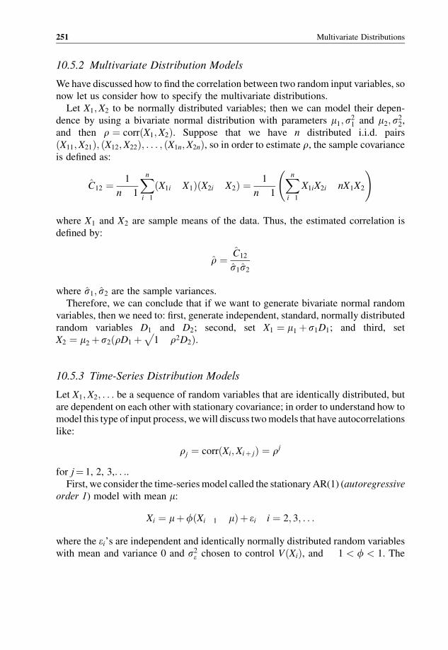
10.5.2 Multivariate Distribution Models
We have discussed how to find the correlation between two random input variables, so
now let us consider how to specify the multivariate distributions.
Let X1;X2 to be normally distributed variables; then we can model their depen-
dence by using a bivariate normal distribution with parameters m1;s21 and m2; s
22,
and then r ¼ corrðX1;X2Þ. Suppose that we have n distributed i.i.d. pairs
ðX11;X21Þ; ðX12;X22Þ; . . . ; ðX1n;X2nÞ, so in order to estimate r, the sample covariance
is defined as:
C12 ¼ 1
n 1
Xni 1
ðX1i X1ÞðX2i X2Þ ¼ 1
n 1
Xni 1
X1iX2i nX1X2
!
where X1 and X2 are sample means of the data. Thus, the estimated correlation is
defined by:
r ¼ C12
s1s2
where s1; s2 are the sample variances.
Therefore, we can conclude that if we want to generate bivariate normal random
variables, then we need to: first, generate independent, standard, normally distributed
random variables D1 and D2; second, set X1 ¼ m1 þ s1D1; and third, set
X2 ¼ m2þ s2ðrD1 þ 1 r2p
D2Þ.
10.5.3 Time-Series Distribution Models
Let X1;X2; . . . be a sequence of random variables that are identically distributed, but
are dependent on each other with stationary covariance; in order to understand how to
model this type of input process, wewill discuss twomodels that have autocorrelations
like:
rj ¼ corrðXi;Xiþ jÞ ¼ rj
for j¼ 1, 2, 3,. . ..First, we consider the time-seriesmodel called the stationaryAR(1) (autoregressive
order 1) model with mean m:
Xi ¼ mþfðXi 1 mÞþ ei i ¼ 2; 3; . . .
where the ei’s are independent and identically normally distributed random variables
with mean and variance 0 and s2e chosen to control VðXiÞ, and 1 < f < 1. The
251 Multivariate Distributions
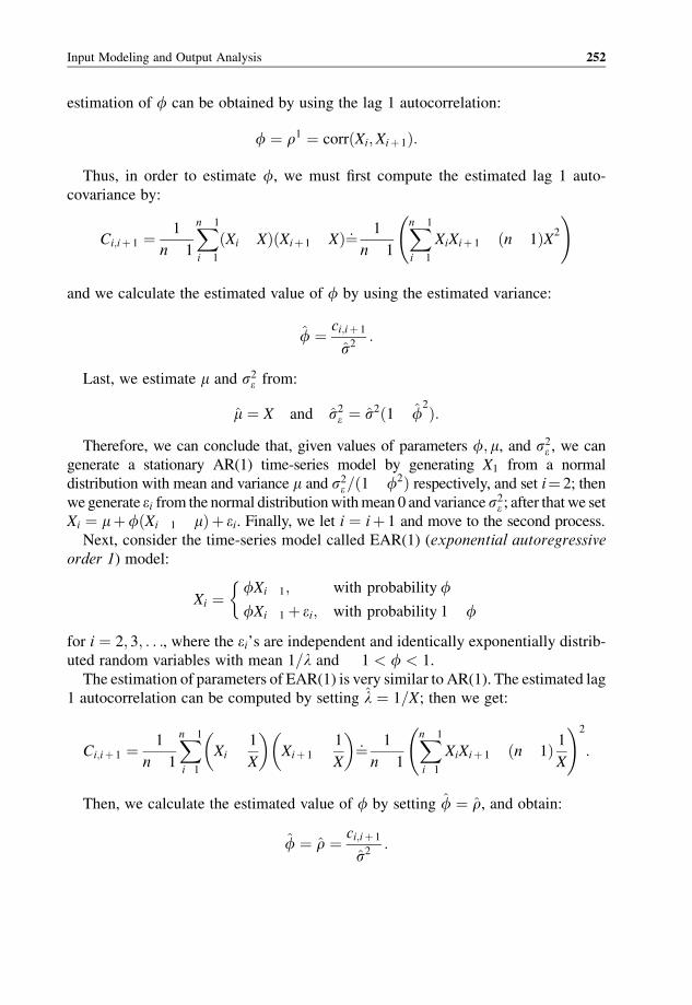
estimation of f can be obtained by using the lag 1 autocorrelation:
f ¼ r1 ¼ corrðXi;Xiþ 1Þ:
Thus, in order to estimate f, we must first compute the estimated lag 1 auto-
covariance by:
Ci;iþ 1 ¼ 1
n 1
Xn 1
i 1
ðXi XÞðXiþ 1 XÞ¼: 1
n 1
Xn 1
i 1
XiXiþ 1 ðn 1ÞX2
!
and we calculate the estimated value of f by using the estimated variance:
f ¼ ci;iþ 1
s2:
Last, we estimate m and s2e from:
m ¼ X and s2e ¼ s2ð1 f2Þ:
Therefore, we can conclude that, given values of parameters f;m, and s2e , we can
generate a stationary AR(1) time-series model by generating X1 from a normal
distribution with mean and variance m and s2e=ð1 f2Þ respectively, and set i¼ 2; then
we generate ei from the normal distributionwithmean 0 and variances2e ; after thatwe setXi ¼ mþfðXi 1 mÞþ ei. Finally, we let i ¼ iþ 1 and move to the second process.
Next, consider the time-series model called EAR(1) (exponential autoregressive
order 1) model:
Xi ¼fXi 1; with probabilityf
fXi 1 þ ei; with probability 1 f
�
for i ¼ 2; 3; . . ., where the ei’s are independent and identically exponentially distrib-
uted random variables with mean 1=l and 1 < f < 1.
The estimation of parameters of EAR(1) is very similar to AR(1). The estimated lag
1 autocorrelation can be computed by setting l ¼ 1=X; then we get:
Ci;iþ 1 ¼ 1
n 1
Xn 1
i 1
Xi
1
X
� �Xiþ 1
1
X
� �¼: 1
n 1
Xn 1
i 1
XiXiþ 1 ðn 1Þ 1X
!2
:
Then, we calculate the estimated value of f by setting f ¼ r, and obtain:
f ¼ r ¼ ci;iþ 1
s2:
Input Modeling and Output Analysis 252
Thus, we can conclude that, given values of the parametersf and l, we can generatea stationary EAR(1) time-series model by generating X1 from an exponential
distribution model with mean 1=l, and set t ¼ 2; then we generate Y from a uniform
distribution model with parameters 0 and 1; if Y � f, then we set Xi ¼ fXi 1, or else
we can generate ei from an exponential distribution with mean 1=l and let
Xi ¼ fXi 1 þ ei. Finally, we let i ¼ iþ 1 and then move to the second process.
10.6 Selecting Distributions without Data
In a real-world scenario, it is often the case that it is not possible to collect data for our
input modeling, so the techniques that we have mentioned in the previous section are
not suitable for the problem of choosing appropriate probability distributions. For
instance, if the system or scenariowewant to simulate is still in the design process and
does not yet exist in concrete form, then it is obvious that collecting data is impossible
for this simulation. How can one model traffic at a gas station before any gas stations
have been built?
Therefore, in such a situation, we must be well prepared and resourceful in
selecting the input process model. In some circumstances, we can obtain informa-
tion on the process in the absence of data by analyzing the nature of the process, such
as inter-arrival times between customers at a specific store. If the customers arrive
one at a time, then wemight think that the inter-arrival times between each customer
are exponentially distributed; or we could make some educated guesses based on
expert opinion by talking to people who are experienced in the particular process,
because they can provide intuition on which the choice of input distribution can be
based.
The uniform, beta, and triangular distributions are often used as the input distribu-
tionwhen data is unavailable because of their characteristics. The uniform distribution
can be a bad choice, because its upper and lower bounds seldomfit the central values in
the real process, so in this case, if the upper and lower bounds are known, the triangular
distribution can be used and the most likely value can be used as the peak of the
distribution.
10.7 Output Analysis
Many simulation studies include randomness in order to get a sense of typical inputs
that the system might face. For example, in the simulation of a processor system, the
processing times required may follow a given probability distribution, or the arrival
times of new jobs may be stochastically defined. Likewise, in a bank simulation,
customers might arrive at random times and the amount of time spent at a teller could
be stochastically determined. Because of the randomness in the components driving a
253 Output Analysis
simulation, its output is also random, so statistical techniques must be used to analyze
the results and aggregate them into meaningful measures from which to draw
conclusions.
The data analysis methods in introductory statistics courses typically assume that
the data is i.i.d. with a normal distribution. Unfortunately, the output data from
simulations is often not i.i.d. and not normal. For example, consider customer waiting
times before seeing a teller in a bank. If one customer has an unusually long waiting
time, then the next customer probably also will, so the waiting times of the two
customers are dependent.Moreover, customers arriving during lunch hourwill usually
have longerwaiting times than customers coming in at other times, sowaiting times are
not identically distributed throughout the day. Finally, waiting times are always
positive and often skewed to the right, with a possible mode at zero, so waiting times
are not normally distributed. For these reasons one often cannot analyze simulation
output using the classical statistical techniques developed for i.i.d. normal data. For
these reasons, more sophisticated statistical methods are needed to examine and
analyze simulation experiments to measure performance.
One of the first steps in any simulation study is choosing the performancemeasure to
calculate. In other words, what measures will be used to evaluate how “good” the
system is. For example, the performance of a queuing systemmay be measured by the
expected number of customers served in a day, or we may use the long-run average
daily cost, or the inverse of the maximum queue size, or the inverse of the mean queue
size as the measure of performance of a supply chain. There are primarily two types of
performance measures for stochastic systems:
1. Transient performance measures, also known as terminating or finite-horizon
measures, which evaluate the system’s evolution over a finite time horizon.
2. Steady-state performance measures, which describe how the system evolves over
an infinite time horizon. These are also known as long-run or infinite-horizon
measures.
10.7.1 Transient Analysis
Transient analysis is an option when we are dealing with a terminating simulation in
which there is a “natural” event B that specifies the length of time for which one is
interested in the system. The event B often occurs either at a time point beyond which
no useful information is obtained, or when the system is “cleaned out.” For example, if
we are interested in the performance of a system during the first 10 time units of
operation in a day, thenBwould denote the event that 10 time units of system time have
elapsed. If we want to determine the first time at which a queue has at least eight
customers, thenB is the event of the first time that the queue length reaches eight. Since
we are interested in the behavior of the system over only a finite time horizon, the
Input Modeling and Output Analysis 254
“initial conditions” I can have a large impact on the performance measure. For
example, queuing simulations often start with no customers present, which would be I
in this setting. In a transient simulation, the goal is to calculate:
m ¼ EðXÞ
where X is a random variable representing the (random) performance of the system
over some finite horizon.
Example 1: Consider a bank line containing an automatic teller machine (ATM).
The line is only open during normal banking business hours, which is 9.00 a.m. to
5.00 p.m., so a customer can access theATMonly during those times.Any customers in
the line at 5.00 p.m. will be allowed to complete their transactions, but no new
customerswill be allowed in. LetZ be the number of customers using theATM in a day.
We are interested in determining the following terminating performance measures:
. E(Z), the expected value of Z. To put things in the framework of (I), we set X¼ Z.
. P{Z� 500}¼E[I(Z� 500)], which is the probability that at least 500 customers use
the ATM in a day, where I(A) is the indicator function of an event A, which takes the
value 1 if A occurs, and 0 otherwise. X¼ I (Z� 500) in this case.
The initial conditions I might be that the system starts out empty each day, and the
terminating event B is that it is past 5.00 p.m. and there are no more customers in the
line.
Alternatively, we might define Z to be the average waiting time (in seconds) of the
first 50 customers in a day. We can then define the following performance measures:
. E(Z), the expected value of Z. In this case, X¼ Z.
. P{Z� 30}¼E[I(Z� 30)], which is the probability that the average waiting time of
the first 50 customers is no more than 30 seconds. Here, X¼ I(Z� 30).
In this case we might specify the initial conditions I to be that the system starts out
empty each day, and the terminating event B is that 50 customers have finished their
waits (if any) in line.
10.7.2 Steady-State Analysis
Now we consider steady-state performance measures. Let Y ¼ ðy1; y2; y3; . . .Þ be a
discrete-time process representing the output of a simulation. For example, if the booth
255 Output Analysis

containing the ATM in the previous example is now open 24 hours a day, then yi might
represent the waiting time of the ith customer since the ATM was installed.
Let FiðY jIÞ ¼ PðYi � yjIÞ for i ¼ 1; 2; . . ., where, as before, I represents the initialconditions of the system at time 0.
Now, ifFiðYjIÞ!FðyÞ! as i!1, thenF(y) is called the steady-state distribution
of the process Y.
Many systems do not have steady-state characteristics. For example, consider
our previous example of an ATM that is accessible only during business hours. Let
Yi be the waiting time of the ith customer to arrive since the ATM was installed.
Then, the process Y does not have a steady state because the first customer of each
day always has no wait, whereas other customers may have to wait. For example,
suppose 500 customers are served on the first day, so the second day begins with
customer 501, who has no wait since there is no one ahead in the line on that day. On
the other hand, if the ATMwere accessible 24 hours a day, then a steady state might
exist.
Consider the ATM discussed earlier, but now suppose that it is accessible all the
time. Let Yi be the number of customers served on the ith day of operation, and suppose
that, over time, the system goes into steady state. We now may be interested in
determining the following steady-state performance measures:
. E(Y), which is the expected steady-state number of customers served in a day.
. P{Y� 400}¼E[I(Y� 400)], which is the steady-state probability that at least 400
customers are served per day.
Again, we may let the initial conditions I denote that the system begins operations
on the first day with no customers present, and, over time, the effects of the initial
conditions “wash away.”
10.8 Summary
This chapter discussed how to deal with data collection as a phase within the network
modeling project life cycle. It lists the different data types that need to be collected to
support network modeling projects, how to collect the data, choose the right distribu-
tion, and validate the correctness of the choice for the kind of distribution that
represents such data.
Recommended Reading
[1] J. Banks, J. S. CarsonII, B. L. Nelson, and D. M. Nicol, Discrete Event System Simulation, 4th
Edition, Pearson Education, 2005.
Input Modeling and Output Analysis 256
[2] O. Balci, “Verification, validation, and certification of modeling and simulation applications,”
Proceedings of the 2003 ACM Winter Simulation Conference ( S. Chick, P. J. Sanchez, D. Ferrin,
and D. J. Morrice, eds.), ACM, 2003, pp. 150 158.
[3] A. M. Law, Simulation Modeling & Analysis, 4th Edition, McGraw Hill, 2006.
[4] L. M. Leemis and S. K. Park, Discrete Event Simulation: A First Course, Prentice Hall, 2006.
[5] B. L. Nelsonnd M. Yamnitsky, “Input modeling tools for complex problems,” Proceedings of the
1998 IEEEWinter Simulation Conference ( D. Medeiros, E.Watson, J. Carson, andM.Manivannan,
eds.), IEEE, 1998, pp. 105 112.
257 Recommended Reading


11
Modeling Network Traffic
11.1 Introduction
As networks are becoming more pervasive, network designers and researchers are
progressively focusing on optimizing network performance and improving network
utilization in terms of throughput, end-to-end delay, packet loss, and other SLA-
related parameters. Network performance and optimization cannot be realized
without a full understanding of network trafficmodeling together with traffic patterns
and traffic generation. In order to generate realistic traffic patterns, mathematical
models should accurately represent the relevant statistical properties of the original
traffic.
Network traffic modeling is essential for theoretical capacity and performance
representation as well as for simulation models. Traffic theory suggests using the
application of mathematical modeling to explain the relationship between traffic
demand and experimental performance. While network traffic models are well
understood for classical networks (e.g., standard assumptions of Poisson arrival rates
and exponential call holding time for the public switched telephone network (PSTN)),
they are more complex for modern high-speed networks where traffic behavior is
difficult to predict. Modern networks exhibit a mixture of traffic types including voice,
data, and video, as well as mobility where the location of nodes and consequently the
source of the traffic are not fixed.
In this chapter, we present several traffic models that are used by simulation
researchers and practitioners to model network traffic loads. It also describes the
most commonly used global optimization techniques to solve optimization problems.
These optimization techniques are useful in modeling and solving complex physical
problems.
Network Modeling and Simulation M. Guizani, A. Rayes, B. Khan and A. Al Fuqaha
� 2010 John Wiley & Sons, Ltd.
11.2 Network Traffic Models
Every few years, the amount of processing speed that one can buy doubles, and the
same holds for memory chips as well. This has been the trend for several decades and
it is expected to keep going for a few decades to come. This encourages customers
to obtain more powerful computers with multimedia capabilities. Consequently,
customers have begun to migrate from text to images, animation, and lately to video,
acquiring high-speed networks capable of supporting new types of services. So the
emergence of new types of services like Cisco’s TelePresence, video conferencing,
video on demand, video telephony, video library, high-definition television (HDTV),
and other services with unknown requirements is expected to be phenomenal in the
future.
Traffic models can be generally divided into two main categories: models which
exhibit long-range dependencies or self-similarities; and Markov models that exhibit
only short-range dependence (Markov chains are discussed in detail in Chapter 9).
Self-similar models include the fractional Brownian motion (FBM) model, on/off
models with heavy-tailed distributions for the on/off duration, and the M/Pareto/
Infiniti models.
Markov models include the traditional on/off models with exponential on/off
distributions, the Markov-modulated Poisson process, and Gaussian autoregressive
models, which typically have exponentially decaying correlation functions.
In the following, we study two traffic models that fall into the second category,
namely constant bit rate and variable bit rate. We also consider one traffic source that
falls into the second category, namely the Pareto traffic (self-similar traffic).
11.2.1 Constant Bit Rate (CBR) Traffic
CBR services generate traffic at a constant rate that can be described simply by their
constant bit rate. The CBR source is not bursty, and the source is active during the
connection (no silent periods). Typical examples of CBR sources include voice, video,
and audio (which requires more bandwidth than voice).
11.2.2 Variable Bit Rate (VBR) Traffic
In this model, traffic is alternating between two states: on and off. Traffic is generated
during the on period at a constant rate, whereas no traffic is generated during the off
period. The length of both periods is exponentially distributed and independent. By
knowing the mean of both on and off periods, different calculations can be obtained
which are useful in trafficmodeling. Typical VBR sources include video-conferencing
and computer network applications. The burstiness of a VBR traffic source is a
Modeling Network Traffic 260
measure of how infrequently a source sends traffic. A source that infrequently sends
traffic is said to be bursty, while a source that always sends traffic at the same rate is said
to be sending at a constant bit rate. The burstiness is defined in terms of the peak rate
and the average rate as:
Burstiness ¼ peak rate=average rate:
11.2.3 Pareto Traffic (Self-similar)
It was demonstrated that Ethernet and World Wide Web (WWW) traffic patterns
are statistically self-similar. An on/off traffic source (VBR traffic source) with a
heavy-tailed distribution, such as the Pareto distribution (discussed in Chapter 7), is
self-similar.
11.3 Traffic Models for Mobile Networks
Evaluating the performance of a mobile ad hoc network depends greatly on the
mobility model used. The mobility model should dictate the movement of the
mobile nodes in a realistic way. Two of the mobility models mostly used by
researchers are the random walk mobility model and the random waypoint mobility
model. Each of these two models generates unrealistic scenarios that make them
inappropriate for mobile ad hoc network simulation. An alternative is to use the
Gauss–Markov mobility model to resolve the problem encountered by the previous
two models.
The randomwalkmobilitymodel was developed tomimic the erraticmovement of
entities in nature that move in unpredictable ways. A mobile node moves from one
location to another by choosing two random values corresponding to speed and
direction. The speed and direction are chosen to be within predefined ranges,
[speedmin, speedmax] and [0, 2p], respectively. After a certain time period t, or
a distance d, new values for the speed and direction are generated. No relation exists
between the current and the past movements of the node. This might lead to
unrealistic scenarios, where a node stops suddenly or makes sharp turns. Also, if
the time period t or the distance d are small values, the node will be moving abruptly
in a small region.
The randomwaypointmobilitymodel uses a pause between changes in speed and/or
direction. A mobile node starts by pausing for a certain time period. Then, it moves
from one location to another by choosing two random values corresponding to speed
and destination. The speed is chosen to be uniformly distributed within [minspeed,
maxspeed]. The mobile node travels toward the new destination at the selected speed.
261 Traffic Models for Mobile Networks
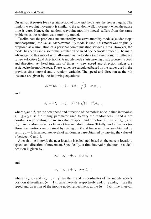
On arrival, it pauses for a certain period of time and then starts the process again. The
randomwaypoint movement is similar to the random walk movement when the pause
time is zero. Hence, the random waypoint mobility model suffers from the same
problems as the random walk mobility model.
To eliminate the problems encountered by these twomobility models (sudden stops
and sharp turns), theGauss–Markovmobilitymodel is used. Thismodelwas originally
proposed as a simulation of a personal communication service (PCS). However, the
model has been used also for the simulation of an ad hoc network protocol. The main
advantage of this model is in allowing past velocities (and directions) to influence
future velocities (and directions). A mobile node starts moving using a current speed
and direction. At fixed intervals of times, n, new speed and direction values are
assigned to themobile node. Thesevalues are calculated based on thevalues used in the
previous time interval and a random variable. The speed and direction at the nth
instance are given by the following equations:
sn ¼ asn 1þð1 aÞsþ ð1 a2Þsxn 1
qand:
dn ¼ adn 1þð1 aÞd þ ð1 a2Þdxn 1
qwhere sn and dn are the new speed and direction of themobile node in time interval n;
a, 0� a� 1, is the tuning parameter used to vary the randomness; s and d are
constants representing the mean value of speed and direction as n!1; sxn 1and
dxn 1are random variables from a Gaussian distribution. Totally random values (or
Brownian motion) are obtained by setting a¼ 0 and linear motions are obtained by
setting a¼ 1. Intermediate levels of randomness are obtained by varying the value of
a between 0 and 1.
At each time interval, the next location is calculated based on the current location,
speed, and direction of movement. Specifically, at time interval n, the mobile node’s
position is given by:
xn ¼ xn 1 þ sn 1cos dn 1
and:
yn ¼ yn 1 þ sn 1sin dn 1
where ðxn; ynÞ and ðxn 1; yn 1Þ are the x and y coordinates of the mobile node’s
position at the nth and (n 1)th time intervals, respectively, and sn 1 and dn 1 are the
speed and direction of the mobile node, respectively, at the (n 1)th time interval.
Modeling Network Traffic 262
The Gauss–Markov mobility model can eliminate the sudden stops and sharp turns
encountered by the models discussed above by allowing past velocities (and direc-
tions) to influence future velocities (and directions).
Next, we discuss the most commonly used global optimization techniques to solve
optimization problems.
11.4 Global Optimization Techniques
Optimization is used by operations researchers and engineers to efficiently design
and evaluate the performance of an overall system. There are well-known algo-
rithms and tools that have been developed to solve specific classes of optimization
problems (e.g., linear programming, integer linear programming (ILP), and convex
programming). Constrained and unconstrained optimization problems appear fre-
quently in many engineering applications. Here, we provide an overview of some of
the most commonly used global optimization techniques for solving constrained and
unconstrained optimization problems and then describe the overall optimization in
mathematics.
11.4.1 Genetic Algorithm
A genetic algorithm is a search algorithm based on the mechanics of natural selection
and natural genetics using the Darwinian principle of reproduction and survival of the
fittest with genetic operations. It was pioneered by John Holland as a modification of
evolutionary programming in the 1960s. The idea is to construct a search algorithm
modeled on the concepts of natural selection in the biological sciences. The process
begins by constructing a random population of possible solutions. This population is
used to create a new generation of possible solutions which is then used to create
another generation of solutions, and so on. The best elements of the current generation
are used to create the next generation. It is hoped that the new generation will contain
“better” solutions than the previous generation and therefore give a better solution
when applied to a practical problem.
11.4.2 Tabu Search
Tabu search is a heuristic procedure for solving optimization problems. It enhances the
searchmethod for finding the best possible solution of a problem. It uses a local search
to repetitively move from a solution x to a solution x0 in the neighborhood of x, untilsome conditions are reached, as shown in Figure 11.1.
The unique contribution of Tabu search is its strategy for escaping local optima in its
search for better solutions. Tabu search is not best described as an algorithm, but as an
263 Global Optimization Techniques
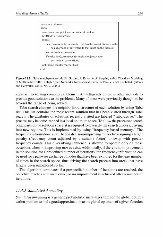
approach to solving complex problems that intelligently employs other methods to
provide good solutions to the problems. Many of these were previously thought to be
beyond the range of being solved.
Tabu search changes the neighborhood structure of each solution by using Tabu
list. This list contains the most recent solution that has been visited through Tabu
search. The attributes of solutions recently visited are labeled “Tabu-active.” The
processmay become trapped in a local optimum space. To allow the process to search
other parts of the solution space, it is required to diversify the search process, driving
into new regions. This is implemented by using “frequency-based memory.” The
frequency information is used to penalize non-improvingmoves by assigning a larger
penalty (frequency count adjusted by a suitable factor) to swap with greater
frequency counts. This diversifying influence is allowed to operate only on those
occasions when no improving moves exist. Additionally, if there is no improvement
in the solution for a predefined number of iterations, the frequency information can
be used for a pairwise exchange of nodes that have been explored for the least number
of times in the search space, thus driving the search process into areas that have
largely been unexplored so far.
The algorithm terminates if a prespecified number of iterations are reached, the
objective reaches a desired value, or no improvement is achieved after a number of
iterations.
11.4.3 Simulated Annealing
Simulated annealing is a generic probabilistic meta-algorithm for the global optimi-
zation problem to find a good approximation to the global optimumof a given function
Figure 11.1 Tabu search pseudo code (M.Guizani, A. Rayes, A.Al Fuqaha, andG.Chaudhry,Modeling
of Multimedia Traffic in High Speed Networks, International Journal of Parallel and Distributed Systems
and Networks, Vol. 3, No. 2, 2000.)
Modeling Network Traffic 264

in a large search space. The term simulated annealing derives from the roughly
analogous physical process of heating and then slowly cooling a substance to obtain a
strong crystalline structure. The main advantages over other local search methods are
that it has more flexibility and the ability to pursue global optimality. It also deals with
highly nonlinear problems.
At each step, the simulated annealing algorithm considers some neighbors of the
current state s in the search space that is analogous to the state of some physical
system and probabilistically decides between moving the system to state s0 at alower energy or staying in the same state. The goal of simulated annealing is to
bring the system from an initial state to a state with the minimum possible energy.
Therefore, the simulated annealing algorithm replaces the current solution by a
random solution chosen with a probability that depends on the difference between
the corresponding function values and on a global parameter temperature that is
gradually decreased during the process. The pseudo code for such a process is
shown in Figure 11.2.
The most significant element of simulated annealing is the random number
generator. It is used to generate random changes in the control variables and for the
increased acceptance test while temperature decreases gradually. A good random
number generator is required to tackle large-scale problems which need thousands of
iterations.
Figure 11.2 Simulated annealing pseudo code (M. Guizani, A. Rayes, A. Al Fuqaha, and G. Chaudhry,
Modeling ofMultimedia Traffic in High Speed Networks, International Journal of Parallel andDistributed
Systems and Networks, Vol. 3, No. 2, 2000.)
265 Global Optimization Techniques
The annealing schedule determines the movements that are permitted during the
search. Thesemovements are critical to the algorithm’s performance. The definition of
annealing schedule is easily stated: the initial temperature should be high enough to
“melt” the system completely and should be reduced toward its “freezing point” as the
search progresses.
The following steps should be specified:
1. An initial temperature T0.
2. A final temperature Tf or a stopping criterion.
3. A rule for decrementing the temperature.
During the search for the best solution, if the solution is improved, the randomly
generated neighboring solution is selected. Otherwise, it is selected with a probability
that depends on the extent to which it decays from the current solution.
The algorithm terminates if it reaches a specified number of iterations, or it reaches a
prespecified minimum at any temperature, or there is no improvement in the solution.
The maximum number of iterations is kept large.
11.5 Particle Swarm Optimization
Particle swarm optimization is a stochastic optimization technique. It bears some
resemblance to evolutionary computation techniques such as genetic algorithms. The
system startswith an initialized population of random solutions for optima by updating
generations. However, unlike genetic algorithms, particle swarm optimization has no
evolutionary operators such as crossover and mutation.
11.5.1 Solving Constrained Optimization ProblemsUsing Particle Swarm Optimization
Swarm intelligence is a kind of artificial intelligence based on the collective behavior
of decentralized, self-organized systems. These systems are modeled by a population
of agents that share information with each other and interact with their environment.
Although there is no centralized control that governs how these agents will interact
with each other, the local, and somehow random, interaction between these agents
leads to a global system intelligence. Examples of these systems are ant colonies,
flocks of birds, and schools of fish.
A number of algorithms were developed and adopted this concept in many
applications. The control of unmanned vehicles in the US Army, planetary mapping
at NASA, crowd simulation inmovies or games, and ant-based routing are examples of
these applications.
Modeling Network Traffic 266

11.6 Optimization in Mathematics
Optimization refers to the study ofminimizing ormaximizing an objective function by
finding the proper values for its variables from within the allowed set of all variables.
Constrained optimization is the minimization of an objective function subject to the
constraints on the values that its variables could have. In general, an optimization
problem can be represented as:
Minimize f ðxÞ; x 2 S � Rn ð11:1Þ
according to the linear or nonlinear constraints:
giðxÞ � 0; i ¼ 1; . . . ;m: ð11:2Þ
The formulation in Equation (11.2) is not restrictive since the inequality can be
represented as gi(x)� 0, and the constraint gi(x)¼ 0 can be decomposed into two
separate constraints, gi(x)� 0 and gi(x)� 0.
Constrained optimization problems can be solved using two approaches. One is the
deterministic approach, such as generalized gradient decent and feasible direction, but
the drawbacks of using such methods is that they require the objective function to be
continuous and differentiable, hence the ongoing research focuses more on using the
other approach, such as stochastic methods like genetic algorithms, evolutionary
programming, and evolutionary strategies.
11.6.1 The Penalty Approach
The most popular way to solve a constrained optimization problem is to use a penalty
function. The search space of the problemcontains two types of points, namely feasible
and infeasible points. Feasible points are those which satisfy all the constraints of the
problem and infeasible ones are those which violate at least one of the problem
constraints.
The penalty approach addresses the optimization problem by transforming it into a
sequence of unconstrained problems by adding a penalty function to the constraints on
the objective function to penalize those points that violate the problem constraints. If
the penalty value is high, the optimization algorithm will settle for finding a local
minimum instead of finding the globalminimum; and if the penalty value is small, then
the algorithm will hardly discover the feasible optimal solution.
The penalty functions can be divided into two categories: stationary and non-
stationary functions. In the former, a fixed penalty is added to the value of the
objective function when a constraint is violated; and in the latter, a dynamically
changed value for the penalty is added depending on how far the infeasible point is
267 Optimization in Mathematics
from the constraint. The literature shows that the results obtained are more accurate
than those obtained using stationary approaches.
The penalty function is:
FðxÞ ¼ f ðxÞþ hðkÞHðxÞ; x 2 S � Rn ð11:3Þwhere f(x) is the objective function in Equation (11.1), h(k) is a dynamically changed
penalty function, and k is the current iteration of the algorithm.H(x) is a penalty factor
defined as:
HðxÞ ¼Xmi 1
YðqiðxÞÞqiðxÞgðqiðxÞÞ ð11:4Þ
where qi(x)¼max{0, gi(x)}, g(qi(x)) is the power of the penalty function,Y(qi(x)) is
a multi-stage assignment function, and gi(x) are the constraints described in
Equation (11.2).
11.6.2 Particle Swarm Optimization (PSO)
Particle swarm optimization (PSO) was developed as a method for optimizing
continuous nonlinear mathematical functions. The ideas for this algorithmwere taken
from artificial intelligence, social psychology, and swarming theory. It simulates
swarms of animals searching for food, like schools of fish and flocks of birds. The
algorithm represents the problem by randomly creating particles which move in the
solution space looking for the particle with the best solution. The algorithm relies on
the concept of information sharing between particles in each program iteration in the
search for the problem optima.
The ith particle of the swarm is represented by the D-dimensional vector Xi¼ (xi1,
xi2, . . ., xiD), the particle’s best position (the position at which the particle had a
minimumvalue for the objective function) is denoted byPi¼ (pi1, pi2, . . ., piD), and thevelocity of each particle is Vi¼ (vi1, vi2, . . ., viD) in a D-dimensional search space.
The movement of a particle in the search space is controlled by the following
movement equations:
Vkþ 1i ¼ xðwVk
i þ c1rki1ðPk
i Xki Þþ c2r
ki2ðPk
g Xki ÞÞ ð11:5Þ
Xkþ 1i ¼ Xk
i þVkþ 1i ð11:6Þ
where i¼ 1, . . ., N and N is the size of the swarm, and where x is a constriction factor
which is used to control and constrict velocities, w is the inertia weight, c1 and c2 are
two positive constants, called the cognitive and social parameter respectively, and ri1and ri2 are random numbers uniformly distributed within the range of [0, 1].
The inertia weight w controls the effect of previous velocities of the particle on its
current velocity. Large values of w facilitate the exploratory abilities of the particle
Modeling Network Traffic 268
while small values allow for exploitation of the local search area. Experimental results
show that it is preferable to setw to a large value at the beginning of the search and then
gradually decrease it when the particle approaches the best fitness value.
The relative magnitudes between r1� c1 and r2� c2 determine whether the particle
moves toward pBest or gBest. If the upper bound of r1� c1 is greater than the upper
bound of r2� c2, then the particle tends to utilize the neighborhood experience more
than its own experience in finding a better fitness value. The values c1 and c2 are
generated randomly for each particle at each iteration so that the particles may vary
their influence among the different sources of information.
11.6.3 The Algorithm
The algorithm for PSO can be written as follows:
For each particle
{
Do
{
Initialize particle
}
}
Do
{
For each particle
{
Calculate the corresponding fitness value
If the fitness value is better than the particle’s best
fitness value
Set the current P vector to the particle’s current X
vector
}
Choose the particle with the lowest fitness value and make it
the global best position
For each particle
{
Calculate the particle’s velocity according to Equation
(11.5)
Update the particle’s current position vector X
}
} while maximum iteration or minimum error criteria is not
attained
269 Optimization in Mathematics
The algorithm starts by creating the swarmof particles and assigning to each particle
its parameters, e.g., its initial position. Then it updates the position of each particle
according to Equations (11.5) and (11.6). At each iteration, the particle compares its
current position to its best ever position. If the current position is better than that
position, the current position becomes the particle’s position. The particlewith the best
value for the fitness function is chosen to be the swarm’s best particle and the particles
in the swarm tend to fly toward this particle.
The main advantages of the PSO are:
1. It does not have many parameters to tune to in order to get an acceptable
performance.
2. It is applicable for both constrained and unconstrained problems.
3. It is easy to implement.
On the other hand, the PSO can converge prematurely if the penalty values are high
and will be trapped in local optima. Also, the parameters are problem dependent and
finding the best values for those parameters is not trivial.
11.7 Summary
In this chapter we studied different traffic models used to simulate network traffic
loads. The models were divided into two main categories: models that exhibit long-
range dependencies or self-similarities; and Markov models that exhibit only
short-range dependence. Self-similar models are typically used to model non-
homogeneous traffic loads, whereas Markov models are used to model traditional
networks such as PSTN.
In the chapter we also introduced the most common optimization algorithms and
tools that have been developed to solve specific classes of optimization problems. We
provided an overview of a few global optimization techniques for solving constrained
and unconstrained optimization problems and then described the overall optimization
in mathematics.
Recommended Reading
[1] J. Banks, Discrete Event System Simulation, 3rd edition, Prentice Hall, 2000.
[2] J. Broch, D. A. Maltz, D. B. Johnson, Y. C. Hu, and J. Jetcheva, “A performance comparison of
multi hop wireless ad hoc network routing protocols,” Proceedings of MobiCom, the ACM
International Conference on Mobile Computing and Networking, Dallas, USA, October 1998.
[3] T. Camp, J. Boleng, and V. Davies, “A survey of mobility models for ad hoc network research,”
Journal of Communication & Mobile Computing (WCMC): Special issue on Mobile Ad Hoc
Networking: Research, Trends and Applications, vol. 2, no. 5, pp. 483 502, 2002.
Modeling Network Traffic 270
[4] D. Johnson and D. Maltz, “Dynamic source routing in ad hoc wireless networks,” in Mobile
Computing (T. Imelinsky and H. Korth, eds.), pp. 153 181, Kluwer Academic, 1996.
[5] A. M. Law andW. D. Kelton, Simulation Modeling and Analysis, 3rd Edition, McGraw Hill, 2000.
[6] B. Liang and Z. Haas, “Predictive distance based mobility management for PCS networks,”
Proceedings of the Joint Conference of the IEEE Computer and Communications Societies
(INFOCOM), March 1999.
[7] M. Zukerman, T. D. Neame, and R.G. Addie, “Internet traffic modeling and future technology
implications,” Proceedings of INFOCOM, 2003.
[8] D. E. McDysan and D. L. Sophn, ATM: Theory and Application, McGraw Hill, 1994.
[9] R. O. Onvural, Asynchronous Transfer Mode Networks: Performance Issues, 2nd Edition, Artech
House, 1995.
[10] R. Gu�erin, H. Ahmadi, and M. Naghshineh, “Equivalent capacity and its application to bandwidth
allocation in high speed networks,” IEEE Journal on Selected Areas inCommunications, vol. 9, no.
7, pp. 968 981, 1991.
[11] W. Willinger, M. Taqqu, R. Sherman, and D. Wilson, “Self similarity through high variability:
statistical analysis of Ethernet LAN traffic at the source level,” IEEE/ACM Transactions on
Networking, vol. 5, no. 1, pp. 71 86, 1997.
[12] M. Guizani and A. Rayes, Designing ATM Switching Networks, McGraw Hill, 1997.
[13] J. Kennedy and R. Eberhart, “Particle swarm optimization,”Proceedings of the IEEE International
Conference on Neural Networks, IEEE, 1995, vol. 4, pp. 1942 1948.
[14] K. Parsopoulos andM.Vrahatis, “Particle swarmoptimizationmethod for constrained optimization
problems,” Frontiers in Artificial Intelligence and Applications, vol. 76, pp. 215 220, 2002.
[15] X. Hu and R. C. Eberhart, “Solving constrained nonlinear optimization problems with particle
swarm optimi zation,” IEEE Conference on Cybernetics and Intelligent Systems, pp. 1 7, June
2006.
271 Recommended Reading

Index
A side, 113 14, 118 19, 121, 126, 185, 189
Academia, 3, 106, 110
Accept reject method, 175 7
Accessible, 108, 203, 256
Accessor, 120, 126, 127, 130, 142
Active response systems, 46, 48
Activities, 23, 24
Actor, 115 17, 120 4, 126, 129, 130,
138, 142
Ad hoc, 68, 105 6, 261 2
Adapter, 115, 117, 125 7, 131, 133, 145,
150, 181
ADS, 98 9
Agent-based, 3, 5
Aggregate Level Simulation Protocol
(ALSP), 5
Aggregate system, 8
Algorithm, 18, 69, 70, 98, 103, 106, 263 70
Analysis, 7, 11, 13, 16 8, 67, 103 5, 122,
157, 253 4
Analytical approach, 11, 246
Analytical modeling, 9, 13, 73
Anderson Darling test (A D test), 248
Aperiodic, 203
API, 104
Appropriate, 8, 15, 17, 27, 60, 69, 105 6,
117, 120, 122 3, 125, 130, 185, 235 8,
240, 245, 248, 253, 261
ARP, 110
Arrivals, 71, 75, 90, 91, 95, 167, 207, 221, 237
ATM, 103, 114, 255 6
Atypical steady states, 14
Autocorrelation, 172, 174, 175, 237, 249 52
Autocorrelation tests, 172, 174
Autocovariance, 250, 252
Autograph, 46
Autopatching, 46
Autoregressive order, 251 2
B side, 113 14, 118 19, 124, 126,
185 7, 189
Banks, 34, 253 5
Baselined, 22
Bed, 1, 98
Behavior, 115 17, 120 31
Bernoulli, 160 2, 201 2
Beta, 235, 253
Binary, 4, 71, 74
Binomial, 160 2, 235, 239, 240
Binomial distribution, 160 2, 239, 240
Birth death process (BD process), 197, 200,
205 6, 226, 232
birthSimEnt() method, 32, 33
Bivariate normal distribution, 251
Bivariate normal random variables, 251
Black-box framework, 115
Boot class, 54, 64
Bottlenecks, 1
Bounds, 187 8, 253
Busy mode, 7, 10
Network Modeling and Simulation M. Guizani, A. Rayes, B. Khan and A. Al Fuqaha
� 2010 John Wiley & Sons, Ltd.
Cþþ , 104
C language, 103, 171
Calibration, 17, 18
Capacity, 6, 7, 72 4, 79, 225 6, 259
Carson, 208, 217, 230
Cartesian lattice, 102
CASiNO, 111 12, 114 17, 127, 131, 136,
140, 149, 154, 169, 181, 187, 208 10, 214,
222, 227, 233
CASiNO framework, 112, 114, 116, 131,
136, 140, 149, 197
CASiNO implementation, 209, 214,
222, 227
CASiNO network simulation, 169
CDF, 73, 158 60, 163 8, 173, 175 8, 245,
247 9
Channels, 10, 98, 113
Chaotic, 5
Chapman Kolmogorov equation
(C K equation), 197, 204 5
Chi-square goodness-of-fit test, 246 8
Chi-square test, 172, 174, 246 8
Chord, 48
Circuits, 98, 103, 226
Clock class, 27, 36, 37
CodeComposer, 98
Coefficient of variation, 240
Coherent lifetime systems, 16
Collaborative intrusion detection, 46
Collapsar, 2
Complexity, 13, 36, 99, 100, 102, 108, 171
Components, 4, 15, 18, 21, 23, 47, 98, 112,
114, 154, 253
Computation, 1, 4
Conduit, 112 30, 137, 140, 142 3, 149 51,
181, 183, 188 90
Conduit framework, 116
Confidence intervals, 219, 231
Connover, 221
Consistency, 17
Constant bit rate (CBR), 260, 261
Content filtering systems, 46
Continuous, 4 5, 15, 71, 157 60, 164, 175,
198 200, 203, 235, 238, 240 2, 246, 247
Continuous distribution, 157, 160, 164, 175,
240, 242, 246
Continuous distribution scenario, 246
Continuous event, 15
Continuous parameter process, 200
Continuous random variables, 160, 164, 242
Continuous state, 4, 5
Continuous time, 4, 197, 201, 203
Continuous-time Markov chains, 197, 201,
203, 260
Control parameters, 16, 103
Conventional, 2, 4, 23, 24
Convergent algorithms, 18
Correlated, 249, 250
Correlation, 14, 159 60, 170, 172, 249 51
Covariance, 159, 160, 249 251
Creator, 117, 129, 130, 149
Cumulative distribution function, 160
Darwinian principle, 263
Data collection, 17, 109, 235 7, 256
Dataflow architecture, 112, 114, 145
deathSimEnt() method, 31, 33
deliveryAck() method, 35, 37, 77, 84
Denumerable, 201
Dependent, 2, 14, 72, 91, 99, 103, 160, 251,
254, 270
deregister() method, 30 33
Descriptive analysis, 19
Design, 1, 2, 5, 8, 9
Design parameters, 16
Detection systems, 46
Deterministic, 5, 18, 69, 95, 198, 267
Development processes, 20, 23
Deviation, 91, 93 5, 165, 166, 173
Device, 2, 17, 102, 111, 112, 204
Diagrammatically, 205
Differential, 4
Discrete, 4, 5, 8, 15, 18, 25, 34, 45, 49, 111,
158 62, 175, 197, 200 1, 203 5, 242, 246
Discrete event, 8, 15, 16, 18, 25, 34, 44, 45,
64, 73, 75, 85, 103 8, 111,131, 154
Discrete-event driven, 98
Discrete-event systems, 16, 108
Index 274
Discrete parameter process, 200
Discrete random variables, 158 60, 232
Discrete scenario, 247
Discrete state, 1, 4
Discrete time, 4, 5, 15
Discrete-time event-driven simulation, 5
Discrete-time Markov chains, 197, 201
Distributed, 5, 46, 47, 69, 73, 79, 107, 112,
164, 166 7, 170, 172, 174, 176 7, 200,
203, 207, 211, 221, 242 3, 251 4,
260 1, 268
Distributed Interactive Simulation (DIS), 5
Distribution, 6 8, 45, 69 75, 94, 102,
157 68, 170, 172 3, 175 9, 181, 183 4,
193, 198, 200, 206 8, 211 12, 216,
235 49, 251 3, 256
DOMINO, 46
Dynamic, 2, 5, 11, 13, 16, 103, 106, 111,
149
Dynamical, 2, 31, 46, 127, 138, 149, 189,
190, 214, 227
EarlyBird, 46
Empirical, 69, 103, 157, 173, 175, 235, 245,
248 9
Empirical CDF, 173, 245, 248 9
Empirical distribution, 175, 235, 248
Empirical distribution function, 248
Emulation, 14, 97
Emulators, 97
Encapsulates, 7
End-to-end, 8, 98, 259
End-to-end delay, 259
Entity, 6
Entry criteria, 21, 22, 24
Env class, 60
Environment, 3, 49, 97 8, 103, 106, 266
Equations, 4, 106, 178, 241 2, 262,
268, 270
Equiprobable approach, 246 7
Ergodicity, 203
Erlang, 235
Ethernet, 103, 261
Evaluation, 8 9, 13, 16, 18, 102
Event, 5 8, 15, 25 7, 29 31, 33 7, 40 1,
44, 49, 51, 57, 60, 64, 66, 76 85, 98, 105,
111, 133, 184 5, 254 5
Event class, 35, 79
Event driven, 5, 8, 15, 98
Event queue, 15
Event routine, 15
Event type, 12
EventHandle class, 27 31
Execution, 26, 31, 38, 66 7, 87, 99, 104, 194
Exit criteria, 21, 22, 24
Experiments, 2, 10, 11, 18, 49, 60, 64, 66 7,
69 70, 74, 90 1, 160, 162, 197, 227, 254,
259, 269
ExpMaker, 190, 192, 193, 214, 227
Exponential autoregressive order, 252
Exponential distribution, 148, 167, 175 7,
181, 184, 193, 197, 206 7, 211, 223, 229,
242, 245, 248, 253
ExponentialBoundedProcess,
187 8, 190 1, 193 4, 222, 227
Exponentially decaying correlation
functions, 260
Exponentially distributed random
variables, 252
ExponentialProcess, 184 8, 190,
191, 209, 214
External, 5, 18, 26, 31, 122
Factory, 6, 76, 115 17, 129 30, 149, 151,
190, 192 3, 214, 227
False aggregation, 237
FDDI, 107 8
FEED HP, 49
Feedback paths, 21, 22
Finite, 15, 97, 108, 158, 160, 170, 188, 201,
221, 248, 254 5
Finite queue, 211, 217, 221
Finite queue length, 221, 254
Finite time horizon, 254
Finite-horizon measures, 254
Finite-state machine, 1, 97, 108
Fitted distribution CDF, 248
Flexible manufacturing system, 16
275 Index
Flow networks, 16
Fractional Brownian motion (FBM), 260
Framework, 8, 18 19, 25, 34, 45, 73 5, 97,
106, 111 12, 114 15, 117, 131, 136, 140,
154, 157, 169, 197, 208, 255
Framework for discrete-event
simulation, 25, 34, 44 5, 111
Freedom, 177, 246
Frequency, 98, 100, 170, 172 175, 238, 240,
241, 246, 247
FSM, 1, 108, 115, 117, 129
Function, 5, 16, 18, 26, 33, 70, 73, 85, 90 1,
103, 115, 140, 158 61, 163 8, 175 8, 199,
238, 242 4, 248 9, 255, 267 8, 270
Gamma, 235 6, 244
Gaussian autoregressive model heavy-tailed
distributions, 260
Genetic algorithm, 69, 263, 266 7
Geometric distribution, 160, 162, 243, 244
Geometrically distributed, 200, 203,
206, 243
Global optimization techniques, 259, 263 6
Gradient estimation, 18
Graphical approach, 244 5
Graphical framework, 18
GUI, 97, 106
HASEþþ , 104
Heavy-tailed distributions, 260 1
‘‘Hello World’’ using the FDES, 34 6
HelloMsg class, 36 8, 40
High-definition television (HDTV), 260
High-Level Architecture (HLA), 5
Honeycomb, 46
Honeypot machines, 47, 67
Host, 5, 46 8, 51 2
Icon-driven interface, 106
Identification, 18
Idle mode, 7
Implemented, 4, 8 9, 28, 45, 48, 73, 75, 80,
103, 108 10, 112, 114, 154, 197, 208, 235,
248, 264
Importance sampling, 69, 175, 177
Independent processes, 200
Independently and identically distributed
(i.i.d.), 240 2, 250 1, 254
Indicator function, 255
Infinite time horizon, 254
Infinite-horizon measures, 254
Initial conditions, 13, 14, 255 6
INITIAL POP, 49
Initialization routine, 15
InitializeVisitors, 193, 214, 227
Input, 1 2, 5, 11, 15 16, 18, 21, 69, 75, 99,
157, 175, 235 8, 240, 244, 249, 251, 253
Input models, 18, 235 6, 244, 249, 253
Input process, 236, 237, 240, 244, 249,
251, 253
Input routine, 15
INSANE, 103
Integral processes, 20
Inter-arrival times, 207, 236, 245, 253
Internal, 5, 17, 25, 27 9, 114,
116, 127
Inter-thread communication, 97
Interval, 7, 15, 69, 79, 86 7, 158, 160 4,
166 8, 170, 177 8, 200, 207, 238, 241,
247, 262
Invalid models, 13
Invariant, 200
Inverse CDF, 73, 245
Inverse transformation, 245
Inversion method, 175 7
IP, 46 9, 97, 110
IP-over-ATM, 103
Iterations, 2, 15, 264 6, 268 70
Java, 25 7, 104, 112, 114, 116, 154, 161 8,
170, 175 6
Joint distribution, 159
Kendall’s notation, 206 8
Kill class, 50 1, 60, 64
Kolmogorov Smirnov test, 172 3, 246
Lag 1, 252
LAN, 103
Index 276
Lexis ratio, 239 40
Linear, 5 6, 106, 160, 170 2, 249, 262 7,
Linear congruential method, 170 2
Linear dependence, 160, 249
Link, 18, 38 42, 98, 109, 207
Link class, 39 43
Little’s law, 206
Little’s theorem, 197, 206
llc sink, 108
llc src, 108
Local, 5, 18, 74, 105, 121, 187, 263 5,
269, 270
Location, 70 1, 200, 245, 259, 261 2
Logic, 5, 9, 32, 48, 64, 114, 116, 127
Logic test, 5
Log-likelihood function, 243
Lognormal, 235
Long-range dependencies models, 260
LossyLink class, 41
MAC, 107 10
Machinery, 2
Main program, 15, 131
Marginal distribution, 159
Markov, 197, 200 1, 203 6
Markov chains, 197, 201 3, 206, 260
Markov models, 260, 270
Markov processes, 200, 201, 203, 205
MATLAB, 3, 98 9, 106, 197, 208, 211, 213,
220, 225, 231 3
Mean, 2, 60, 70, 73, 75, 91 5, 102, 112,
160 6, 168 9, 174, 176 8, 187, 195,
207, 211 12, 216 18, 223 4, 226,
229, 230, 236, 238, 240 2, 248, 251 4,
260, 262
Median, 238
Memoryless, 203, 206
Meta-modeling, 18
Method of moments, 241 4
Methodology, 1, 10, 16, 24
MLE, 242
Model, 1 6, 9 11, 13 18, 21 4, 26, 69, 79,
97, 99 100, 103 10, 157, 167 8, 184,
187 8, 197, 207 9, 211 14, 217, 220 1,
224, 226 7, 230 1, 235 7, 241, 249,
251 3, 259
Model-based design, 106
Modeling, 1 3, 6, 8 9, 13 14, 18, 24, 49, 73,
94, 97 100, 101 7, 109 10, 157, 235, 244,
249, 253, 256, 259 60
Model validation, 17
Modulated Poisson process heavy-tailed
distributions, 260
Module, 97, 101, 103, 108 12, 114, 184,
209, 214, 222, 227
Modulus, 170, 172
Monte Carlo (MC), 5, 8, 9, 14, 69 75, 90,
95 6
Monte Carlo simulation, 8, 14, 69 75, 77,
90, 95
MOOSE, 103
Multiple steps transition, 204
Multiple-output queue, 219
Multiplicative congruential method, 170
Multivariate distribution models, 251
Multivariate distributions, 249 53
Mux, 115 17, 120, 123, 126, 128, 142 5,
149 51, 188 9, 192 4, 214, 227
MySink, 131, 133, 137, 140, 145, 150,
192, 194, 209 10, 214 15, 222 3, 227 8
MySink module, 209, 214, 222, 227
Native programming code, 97
NetSim, 103, 110
Network, 5, 25, 42, 44 9, 51, 54, 56 7,
59 60, 62, 64, 66 8, 97 8, 100, 102 3,
105 13, 115, 133, 154 5, 169, 181, 195,
206, 235, 256, 259
Network links, 206
Network performance, 259
Network systems, 259 62
Network utilization, 259
Node class, 36
Non-parametric, 236
Normal distribution, 94, 102, 162, 165 6,
177 8, 241 2, 251 2, 254
Normal random variables, 251
ns2, 98, 105 6, 110
277 Index
N-step transition probabilities, 204
Null hypothesis, 246, 249
On/off models with exponential on/off
distributions, 260
On/off models with heavy-tailed
distributions, 260 1
One-step transition probabilities, 204
OPNET, 98 9, 103 4, 106 10
Optimal selection, 16
Optimization, 17 9, 73 4, 97, 110, 259,
263 4, 266 70
Ordinary, 4, 49, 106
OSI, 107, 109
Output analysis, 18, 67, 105, 231, 253 6
Packet, 42 3, 46 8, 97 8, 100, 103, 108 9,
112, 116, 134 5, 138, 141 2, 146 8, 151 3,
181, 183 7, 193 5, 207, 209, 211, 216,
222 3, 229, 259
Packet delay, 207
Packet loss, 259
Packet processing, 183, 207
Packet processing delay time, 207
Pairwise influences, 264
Parameter values, 13, 16, 18, 67, 244
Pareto distribution, 168 9, 261
Pareto traffic, 260 1
Particle swarm optimization, 266, 268
PDE, 101
PDF, 158, 163 8, 177, 238, 242
PEER H, 49
Penalty approach, 267 8
Performance evaluation, 8 16, 18,
84, 102
Performance evaluation technique
(PET), 8 15
Performance measure, 8 10, 16, 18, 60, 67,
69 70, 72 5, 78, 81, 90, 94 5, 99, 187,
254 6
Periodicity, 203
Perturbations, 16
Petri dish, 45
PHY, 107
phy rx, 108
phy tx, 108
Pitfalls, 13 4, 237
PMD, 107
PMF, 238, 242 3
Poisson distribution, 160, 163, 181, 183,
239
Poisson process, 193 4, 197, 206 7,
211 12, 215, 221, 223, 226, 229, 260
PoissonSource, 182 3, 192 4, 214 15,
222, 227
Population, 69, 95, 102, 165, 168, 205 6,
241, 263, 266
Positive recurrent, 203
Post-prescriptive analysis, 19
Potemkin, 47
P P (probability probability), 244, 246
Preemption of events, 224
Prescriptive analysis, 19
Private server, 226
PRM PROB VULNERABLE, 49 50
Probabilistic, 5 6, 14 15, 18, 69, 95,
236, 264
Probability density function, 158, 238
Problem formulation, 16
Process, 1 2, 6 11, 14, 16 21, 37, 46, 48,
69, 99, 100 4, 106 8, 116, 125 6, 130,
154, 157, 173, 176, 181, 184 91,
193 4, 197 201, 203, 205 8, 211 12,
214 16, 221, 223, 226, 229, 232, 235,
237 8, 244, 247, 249, 251 3, 255 6,
260, 262 5
ProcessorSubsystem, 217, 230
ProcessorSubsystem main class, 230
Processor system, 253
Production, 1 2, 16
Production lines, 16
Project support processes, 20
Propagation medium, 98
Properties, 9, 18, 69, 74, 95, 149, 158 9,
165, 172, 197, 203, 206, 209, 213, 221,
226 7, 247 9, 259
Properties of Markov chains, 197, 203
Proto-C, 103
Index 278
Protocol, 5, 36, 97 8, 102 5, 107, 109 10,
112 15, 117, 128 9, 135 8, 140, 142,
145, 149 50, 154, 181, 183, 187,
190, 193 4
PSpice, 98
Q Q (quantile quantile), 237, 244 6, 248
Quality, 2, 105, 244
Quantile quantile plot, 237, 244 6
Quantile value, 245
Queue, 5 9, 15, 72, 74, 80 1, 83, 87, 90, 109,
154, 184 8, 193, 195, 198, 206 9, 211 14,
217, 219 27, 230 1, 254
Queue class, 211, 217, 219, 224, 230
Queue size, 72, 74, 87, 90, 186, 193, 195,
211, 254
Queuing system, 197, 205 6, 209, 214, 222,
227, 254
Queuing theory, 9, 181, 197 233
Ragged, 238 9
Random, 5 8, 10, 14, 18, 41, 48 51, 56 7,
64, 69 73, 79, 90 1, 93, 95, 102, 105,
157 79, 181, 184, 193, 198 200, 202 3,
206 8, 232, 235 6, 241 2, 245, 247,
249 55, 261 3, 265 6, 268
Random number generators, 5, 14, 69, 95,
105, 157, 172, 179, 265
Random realization, 7
Random sequence, 69, 91, 200
Random variable, 6, 8, 72, 158 68, 170, 173,
175 7, 198 200, 202 3, 206, 232, 235,
241 2, 245, 249 52, 255, 262
Random variate, 6, 163, 169, 175, 177, 184,
236
Random variate generation, 163, 175 9
Random walks, 69, 200, 261 2
Rayleigh distribution, 166 7, 178 9
RCSP, 103
Reachable, 117, 203
REAL, 103, 105, 110
Real trace data, 7
Reality, 3, 10, 11, 17, 69
Real-life simulation, 209, 213, 221, 227
recv() method, 30, 36, 39, 49 51, 60, 78,
81, 84, 87, 181, 183
register() method, 30
Report generating, 18
Report generation routine, 15
Reverse transition, 206
revokeSend() method, 33
RF channels, 98
RoundRobin mux, 190, 192 4, 214,
227
SAAL, 113 14
Scale parameters, 245
SCAN PERIOD, 49
Scenarios, 1, 4, 18, 71, 103, 238, 246 7, 250,
253, 261
Scheduler class, 26, 112
Scheduling, 6, 8
Schematic, 18
Self-similarities models, 260
Semi-Markov processes, 200
send() method, 35
Sensitivity analysis, 16, 18, 67
Sensitivity estimation, 18
Sequence, 5, 10, 19, 46, 69, 71, 75,
90 1, 95, 133 4, 139, 157, 161 2,
170 2, 174, 185, 200, 202 4, 235,
237, 251, 267
Sequencing, 22, 72
Server, 6 8, 10, 13, 72, 75, 80, 82 7, 89 91,
93 5, 209, 211 13, 216 17, 220 1, 224,
226, 229 31, 236
Service level agreement (SLA), 259
Service time distribution, 208
Short-range dependence models, 260
SIMþþ , 104
SimEnt class, 26, 32 5, 49
Sim Event, 211, 220, 231
Sim hold(), 105
SimJava, 104 5, 110, 197, 208, 211 12,
217, 224, 230, 232 3
SimJava implementation, 211 12, 217, 224,
230, 232
SimJava package, 105, 197
279 Index
SimJava tutorial, 104 5, 211 12, 217, 224,
230, 232 3
Sim schedule(), 105
Sim select(), 105
Sim trace(), 105
Simulated annealing, 69, 264 6
Simulation, 1 19, 25 6, 30 2, 34 5, 44 5,
49 51, 53 4, 60, 62, 64, 66 75, 79, 85,
88 91, 93, 95, 97 107, 110 12, 120,
122 5, 131, 133, 154, 157, 169, 179,
181, 184, 192 3, 195, 197, 200, 204,
206, 208 11, 213 14, 217 18, 221 2,
227, 230, 231, 233, 235 6, 253 5, 259,
262, 266
Simulation clock, 15
Simulation model development, 17
Simulation modeling, 3, 6, 9, 13, 49 65
Simulators, 5, 10, 25, 49, 97, 103, 105 6,
110, 112, 157
Simulink, 106, 110
Simulink/MATLAB, 98
Sim wait(), 105
Sink, 126, 131, 225
Skewness, 240
Software lifetime cycle model (SLCM),
18 19
Source class, 211
Specification, 21 2, 34, 103, 111, 116, 121,
125, 129 30, 133
Splitting, 70
SPW, 98
SSCOP, 113 14
Standard queuing notation, 207 8
State variables, 4, 6, 13, 15
Statement of work (SOW), 21 2, 24
Stationary autoregressive order, 1, 251
Stationary exponential autoregressive
order, 1, 252
Stationary processes, 200
Stationary transition probabilities, 201
Statistical, 7, 9, 15, 18, 49, 69, 74, 95, 105,
157, 160, 170, 176 7, 179, 187, 246, 249,
254, 259
Statistical distribution function, 176 7
STD, 107 9
Steady-state characteristics, 256
Steady-state inputs, 209, 214, 221, 227
Stochastic, 16, 18, 197 8, 200, 203, 235,
254, 266 7
Stochastic process, 197 8, 200,
203, 235
Subnet link, 207
Swarm intelligence, 266
Symmetric, 165, 177, 238, 250
Tabu search, 263 4
Tasks, 23 4, 105 6
TCP, 47 8, 105, 110
Technique, 1 2, 8 9, 14, 16, 18, 69, 95, 157,
233, 240 2, 244, 246 8, 253 4, 259, 263,
265, 270
TelePresence, 260
Thermal noise, 10
Throughput, 221, 226, 259
Time distribution, 208
Time driven, 15
Time-series distribution models, 251
Trace driven, 15
Tradeoff, 17 18, 95
Traffic generator, 6 7, 76, 181
Traffic systems, 16
Trance drive, 210
Transient, 75, 113, 116, 121, 203,
254 5
Transient analysis, 254
Transient performance measures, 254
Transient simulation, 255
Transition probability matrix,
201 2
Transmitting, 26, 53, 204
Traveling sales person (TSP), 177
Trials, 91, 93 5, 160 1, 201 2
Triangular distribution, 175, 253
Tutorial, 25, 34 43, 131 153, 181,
183, 188
Typical stochastic system, 16
Index 280

Uncorrelated, 166, 250
Uniformdistribution, 7, 73, 164, 172 3, 175,
240, 253
Uniformly distributed, 73, 79, 164, 170, 172,
174, 176 7, 261, 268
UniqueDouble class, 27 8
Univariate distribution, 240, 249
Unverified models, 13
Utilization factor, 209
Validation, 17, 79, 100
Variable, 4, 6, 8, 13, 15, 32, 77 8, 85,
158 68, 170, 173, 175 8, 198 203, 206,
232, 235, 237, 241, 242, 245, 249 52, 255,
260, 262, 265, 267
Variable bit rate (VBR), 260
Variance, 75, 91, 93, 95, 161 8, 174, 207,
239 42, 249, 251 2
Verification, 17, 106
Video conferencing, 260
Video library, 260
Video on demand, 260
Video telephony, 260
Virtual, 1, 9, 103
Weibull, 175, 235
‘‘What-if’’ analysis, 2, 18
While statement, 224
White-box framework, 115
Work flow, 21, 22
Work units, 19, 21 3
281 Index