HAL Id: hal-00714386https://hal.inria.fr/hal-00714386

Submitted on 31 Oct 2013

HAL is a multi-disciplinary open accessarchive for the deposit and dissemination of sci-entific research documents, whether they are pub-lished or not. The documents may come fromteaching and research institutions in France orabroad, or from public or private research centers.

L’archive ouverte pluridisciplinaire HAL, estdestinée au dépôt et à la diffusion de documentsscientifiques de niveau recherche, publiés ou non,émanant des établissements d’enseignement et derecherche français ou étrangers, des laboratoirespublics ou privés.

Network design for mesoscale inversions of CO2 sourcesand sinks

Thomas Lauvaux, Andrew E. Schuh, Marc Bocquet, Lin Wu, ScottRichardson, Natasha Miles, Kenneth J. Davis

To cite this version:Thomas Lauvaux, Andrew E. Schuh, Marc Bocquet, Lin Wu, Scott Richardson, et al.. Network designfor mesoscale inversions of CO2 sources and sinks. Tellus B - Chemical and Physical Meteorology,Taylor & Francis, 2012, 64, �10.3402/tellusb.v64i0.17980�. �hal-00714386�

Network design for mesoscale inversions of CO2 sources

and sinks

By T. LAUVAUX1*, A. E. SCHUH2 ,5 , M. BOCQUET3 , L. WU3 , 4 , S . RICHARDSON1 ,

N. MILES1 and K. J. DAVIS1 , 1Department of Meteorology, The Pennsylvania State University,

University Park, TX, USA; 2Natural Resource Ecology Laboratory, Colorado State University, Fort Collins, CO,

USA; 3CEREA, Joint Laboratory Ecole Nationale des Ponts et Chaussees/EDF R&D, Champs sur Marne,

France; 4Laboratoire des Sciences du Climat et de l’Environnement, IPSL-LS, CECEA-CNRS-UVSQ,

UMR8212, Saclay, France; 5Department of Atmospheric Science, Colorado State University, Fort

Collins, CO, USA

(Manuscript received 4 March 2012; in final form 26 April 2012)

ABSTRACT

Recent instrumental deployments of regional observation networks of atmospheric CO2mixing ratios have been

used to constrain carbon sources and sinks using inversion methodologies. In this study, we performed

sensitivity experiments using observation sites from the Mid Continent Intensive experiment to evaluate the

required spatial density and locations of CO2 concentration towers based on flux corrections and error reduction

analysis. In addition, we investigated the impact of prior flux error structures with different correlation lengths

and biome information. We show here that, while the regional carbon balance converged to similar annual

estimates using only two concentration towers over the region, additional sites were necessary to retrieve the

spatial flux distribution of our reference case (using the entire network of eight towers). Local flux corrections

required the presence of observation sites in their vicinity, suggesting that each tower was only able to retrieve

major corrections within a hundred of kilometres around, despite the introduction of spatial correlation lengths

(�100 to 300 km) in the prior flux errors. We then quantified and evaluated the impact of the spatial correlations

in the prior flux errors by estimating the improvement in the CO2 model-data mismatch of the towers not

included in the inversion. The overall gain across the domain increased with the correlation length, up to 300 km,

including both biome-related and non-biome-related structures. However, the spatial variability at smaller scales

was not improved. We conclude that the placement of observation towers around major sources and sinks is

critical for regional-scale inversions in order to obtain reliable flux distributions in space. Sparser networks seem

sufficient to assess the overall regional carbon budget with the support of flux error correlations, indicating that

regional signals can be recovered using hourly mixing ratios. However, the smaller spatial structures in the

posterior fluxes are highly constrained by assumed prior flux error correlation lengths, with no significant

improvement at only a few hundreds of kilometres away from the observation sites.

Keywords: carbon dioxide, atmospheric inversion, air�land interaction, mesoscale modelling, carbon cycle,

data assimilation

1. Introduction

The remaining fraction of atmospheric carbon from

anthropogenic emissions corresponds to about 45% of

the total emissions, due to absorption mechanisms on the

continents and the oceans (Raupach et al., 2008; LeQuere

et al., 2009). Although anthropogenic emissions are re-

ported with high accuracy at the national level (Gurney

et al., 2009), the role of continental surfaces affected by

a large interannual variability remains critical to better

understand and predict the atmospheric accumulation

(Canadell et al., 2007). Their contribution remains poorly

constrained at the continental and regional levels using

inverse approaches despite consistency at larger scales

(Ciais et al., 2010). Process-based approaches and statis-

tical regression methods for parameter optimisation have

also been used to constrain the carbon pools and the net

flux from the terrestrial vegetation (Ricciuto et al., 2011),*Corresponding author.

email: lauvaux@meteo.psu.edu

Tellus B 2012. # 2012 T. Lauvaux et al. This is an Open Access article distributed under the terms of the Creative Commons Attribution-Noncommercial 3.0

Unported License (http://creativecommons.org/licenses/by-nc/3.0/), permitting all non-commercial use, distribution, and reproduction in any medium, provided

the original work is properly cited.

1

Citation: Tellus B 2012, 64, 17980, http://dx.doi.org/10.3402/tellusb.v64i0.17980

P U B L I S H E D B Y T H E I N T E R N A T I O N A L M E T E O R O L O G I C A L I N S T I T U T E I N S T O C K H O L M

SERIES B

CHEMICAL

AND PHYSICAL

METEOROLOGY

(page number not for citation purpose)

but large discrepancies remain on the annual and seasonal

time scales (Keenan et al., 2012).

Because of the absence of direct measurements of

regional carbon fluxes, the evaluation of the methods at

policy relevant scales (few 10ths of kilometres) is limited to

intermodel comparisons (Schwalm et al., 2010) and un-

certainty analysis of parameters (Knorr and Heimann,

2001) or based on direct or indirect measurements (Wang

et al., 2001). The Mid Continent Intensive (MCI) experi-

ment focused on an intensively managed area for which

agricultural inventories can provide reliable annual flux

estimates (West et al., 2011), primarily driven by harvest

production of crops. The inventory product can be used to

evaluate other carbon flux estimates from biogeochemical

terrestrial models, model-data fusion approaches, or atmo-

spheric inversions. Despite the high precision obtained

in the inventories from the collected crop harvest data

(Ogle et al., 2010), the uncertainty over the entire region

is increased by lower sampling frequency in the forest

inventory, the parameterisations involved in the inven-

tory models, the high variability from natural ecosystems

and poorly documented semi-managed ecosystems such as

pasture.

Mesoscale atmospheric inversions were used in several

studies as a promising tool to monitor and estimate

regional flux balances at high resolution (Lauvaux et al.,

2009; Schuh et al., 2010; Gockede et al., 2010a). Though

errors in the atmospheric transport model and at the

boundaries limit the potential of the method (Gockede

et al., 2010b; Lauvaux et al., 2012), mesoscale inverse sys-

tems have shown consistent improvements from prior

fluxes over short periods of time (Lauvaux et al., 2009),

and at the annual time scale over the region (Schuh et al.,

2010). Over longer time scales, the assessment of the

regional flux balance implies the capability of capturing

the spatio-temporal variability in the atmospheric CO2

mixing ratios and avoiding persistent errors from the

atmospheric transport models (e.g. Gerbig et al. 2006).

Although prior fluxes, uncertainty assessment and trans-

port models are evaluative components of the system, the

deployment strategy of observation sites affects the poten-

tial of the inversion indefinitely.

The design of regional atmospheric networks amounts

to the optimisation of the observational constraint on the

surface fluxes from the atmospheric concentrations. The

atmospheric integrator effect is one part of the answer, and

actual footprints of hourly tower concentration data were

shown to constrain mainly the few hundreds of kilometres

around each site (Lauvaux et al., 2008; Gerbig et al., 2009).

Even though large-scale signals are present in the concen-

trations, their relative contribution being 20�40% (depend-

ing on the season) of the observed hourly variability (Miles

et al., 2012), but the corresponding flux area is so large that

very little information is carried by the data to constrain

the flux per surface unit. In addition, CO2 fluxes show large

diurnal patterns varying from negative values during the

day to positive during the night (photosynthesis and

respiration), resulting in a substantial loss of information

at the daily time scale (Gerbig et al., 2009). Still, regional-

scale signals and redundant flux signatures in the atmo-

spheric concentrations might inform us about larger flux

balances, depending on the site location and the strength of

the local fluxes.

Previous studies have demonstrated the relative contri-

bution of the near-field fluxes in the hourly atmospheric

observations using a limited number of observation sites

deployed over short periods of time (Lauvaux et al., 2009).

Other studies have used similar modelling tools at coarser

resolution but for non-CO2 trace gases, i.e. those not af-

fected by diurnal cycles, and limited by the resolution to

extract the high time frequency atmospheric information

from the observations (Gloor et al., 2001). In addition to

the use of high-frequency data, the a priori flux spatial

distribution in the region of interest is the second major

element. Once combined in the inverse system, both deter-

mine the potential of convergence to assess the regional

carbon balance and the capability to retrieve the correct

spatial flux distribution. The convergence of the system is

directly related to the spatial and temporal resolutions of

the aggregated fluxes. The aim is to constrain the surface

fluxes which is different from observing signals from

different scales in the observations. The relative contribu-

tion of one scale can limit the use of the others. A crucial

element of the inverse system concerns the detection

of major discrepancies in the prior fluxes. These are not

detectable by any pseudo-data sensitivity study without

prior knowledge of potential biases or errors in the prior

fluxes. If towers are to be deployed, the design of the

network is based on its ability to capture surface flux

discrepancies at any place in the domain. Networks that are

too sparse might have limited potential, whereas too dense

networks are cost-prohibitive and harder to maintain on a

long-term basis. Basically, the distance between observa-

tion sites and critical flux areas has to be determined within

an inverse framework, such that atmospheric signals are

strong enough to optimise the regional fluxes relatively to

other contributors.

We propose here a set of tests based on previous results

over the MCI area (Lauvaux et al., 2012) using different

combinations of tower sites, considering their impacts

on the regional flux balance and its spatial distribution.

We focus on June to December 2007 which allows us to

(1) evaluate the weight of the observations from each site to

help constrain the regional carbon balance and its spatial

distribution and (2) investigate the impact of different prior

error statistics that may be used in network design studies

2 T. LAUVAUX ET AL.

and evaluate our own assumptions. This step is critical

before using the error reduction as a reliable estimate for

network design purposes; furthermore, a large correlation

length in the prior flux errors can lead to over-constrained

systems (or under-estimated posterior uncertainties).

2. Methods

2.1. The campaign and the modelling tools

For this study, we used eight CO2 mixing ratio tower sites

that were deployed for the MCI experiment (Miles et al.,

2012). Two towers are part of the permanent tall tower

NOAA network, LEF and WBI; five sites were instru-

mented for the campaign, Kewanee, Round Lake, Mead,

Galesville, Centerville; and the last site is the calibrated flux

tower Missouri Ozarks [cf. Fig. 1(a)]. The inverse system,

described in a previous study (Lauvaux et al., 2012), uses

WRF-Chem meteorological fields at 10 km resolution to

drive the Lagrangian Particle Dispersion Model (Uliasz,

1994) and generates the concentration footprints over

the entire period of observations. The prior fluxes were

simulated with the SiBcrop model, with an improved

phenology for crops based on several eddy-flux sites over

the MCI (Lokupitiya et al., 2009). The inverse CO2 fluxes

are at 20 km resolution over the domain at a weekly time

step. We solve for two flux components (one for daytime

and one for nighttime). We also solve for boundary

condition concentrations from the CarbonTracker system

corrected by aircraft data (Lauvaux et al., 2012). The

boundary conditions are additional unknowns here but

in practice act as an additional source of uncertainties,

reducing the overall error reduction of the different cases

equally.

2.2. Inverse methodology

The method used in the paper was described in the study

of Lauvaux et al. (2012). The state vector (x) that includes

the three components described above (daytime fluxes,

nighttime fluxes and boundary inflow) is obtained by the

following equation:

x ¼ x0 þ BHT ðHBHT þ RÞ�1ðy �Hx0Þ (1)

where x are the unknown fluxes and the boundary

conditions we invert for, x0 the a priori flux and boundary

estimates, y the observations, H the linearised transport

matrix and R and B the error covariance matrices of the

observations and the a priori fluxes, respectively.

We can define the posterior error covariance matrix A

for fluxes given by the following expression:

A�1 ¼ B�1 þHTR�1H (2)

In the study, we perform error reduction analyses as if

exploring optimal tower locations for a network design

study. The error reduction is the ratio between flux error

variances before and after inversion [1� ðrA=r

BÞ] with

values ranging from 0 to 1, with sA the posterior flux root

mean square error (RMSE) and sB the prior flux RMSE.

A value of 0 indicates no improvement of the initial prior

errors. Between 0 and 1, the value is interpreted as a ratio

of error reduction, referred in percentage in this study.

In addition, we define prior flux error structures in

two different ways: first by considering the ecosystem dis-

tribution in space and a correlation length L, and second

only by the correlation length L (Lauvaux et al., 2012).

The distance L remains difficult to rigorously estimate but

its impact on the retrieved fluxes can be large (Wu et al.,

2011). Additional tests will be performed based on our

subsampled network inversions, to evaluate the impact of

the flux corrections on the CO2 concentration mismatch of

the observation sites not used in the inversion.

2.3. Evaluation of the assumptions in spatial

structures of the prior flux errors

2.3.1. Ratio between the observational constraint and

prior flux errors. To evaluate the impact of the correla-

tion structures on the solutions, we use the degree of

freedom for the signal (DFS) from Rodgers (2000). A large

(respectively, small) correlation length reduces (respec-

tively, increases) the DFS. The DFS was defined following

Bocquet (2009) as:

DFS ¼ TrðBHT ðHBHT þ RÞ�1HÞ (3)

The DFS is used in this study to investigate the impact of

the correlation length on the solutions. Small DFS values

compared to the number of observations indicates that

the posterior fluxes are constrained mainly by the prior

uncertainties. Large correlation lengths lead to less infor-

mation brought by the observations. We discuss the DFS

values in Section 4.

The variances in the prior flux errors vary slightly from

one case to the next to conserve the same ratio between the

observational constraint and the prior flux uncertainties.

This balance was ensured by estimating the normalised

distance l of the x2 test as follows:

k ¼1

n½ðy �Hx0Þ

TðHBHT þ RÞ�1ðy �Hx0Þ� (4)

with n the degree of freedom of the state vector. A value

close to one indicates reasonable estimates of prior errors in

the inverse system, balancing the weight of the atmospheric

observations and their related errors (y and R) compared

with the initial uncertainties in the fluxes (x0 and B) and

NETWORK DESIGN FOR CO2 FLUX MESOSCALE INVERSIONS 3

(a) Prior fluxes from SiBcrop (b) Inversion TR0: Complete network of towers

(c) Inv. NON-CORN: no Corn Belt sites (d) Inv. CORN: Corn Belt sites only

(e) Inv. SPARSE: Sparser network (f) Inv. MIN: Minimal network

Fig. 1. CO2 fluxes from June to December in TgC.degree�2 over the MCI from the SiBcrop vegetation model (a), our reference case

TR0, i.e. the inverse system using the entire network of observation sites (b), using only the sites outside of the Corn Belt area (c), using the

sites only within the Corn Belt area (d), using a sparser network (e) and using a minimal configuration of two sites (one in the Corn Belt and

one out) (f).

4 T. LAUVAUX ET AL.

the number of independent elements in the state vector. The

values of l range between 0.75 and 1.25 for all our tests, and

the corresponding correlation lengths from 50 to 300 km,

including both biome-dependent and non-biome-dependent

structures. We increase (or decrease) the RMS (diagonal

elements of B) to compensate for changes in the correlation

length based on the values of lambda for each case.

2.3.2. Leave-One-Out Cross-Validation. We evaluated

the gain from the inversion in terms of mixing ratio

mismatch with Leave-One-Out Cross-Validation (LOOCV)

tests. We performed eight consecutive inversions using

seven of the eight available tower sites. The remaining site

is used as a validation of the inverse fluxes. The simulated

mixing ratios of the validation site are reconstructed using

its influence functions and the fluxes from the correspond-

ing 7-tower inversion. The mixing ratio mismatch at the

validation site i (Di�y�Hxj) is computed before (xj�x0)

and after inversion (xj�x). The mean of the mismatch

represents the impact of the correction of weekly biases

in the observation space (mixing ratios). The RMSE of

hourly mismatches represents smaller-scale corrections

(from hourly mixing ratios) produced by changing wind

conditions at each site. These tests provide an assessment of

the overall gain after inversion, gain from corrections on

the weekly fluxes and in space around the validation site.

Considering that most tower mixing ratio footprints do not

overlap between sites, the LOOCV evaluates primarily the

veracity of the spatial correlation in the prior flux errors.

3. Results

The amount of information from the observation network

varies with two major elements: the spatial density of

the network and the correlations of the prior flux errors.

To explore these two components, first we define several

subnetworks using only some of the eight available sites,

and second, we assume different prior flux error structures

with an evaluation of their impact.

3.1. Regional CO2 flux balance

In this section, we diagnose the information content of

the observations using different combinations of sites to

constrain the regional balance. We defined four cases as

follows: the first network excludes sites in the corn belt

(Round Lake, West Branch and Kewanee) referred here

as NON-CORN; the second case uses sites within the

corn belt only (the ones precedently excluded) referred

as CORN; a sparser network of observations but homo-

geneously distributed in space (excluding Centerville,

Galesville and Kewanee) referred as SPARSE; and finally

the minimum configuration with one site in the corn belt

area and one for the mixed grassland-crop-forest area,

Round Lake and Centerville, referred as MIN.

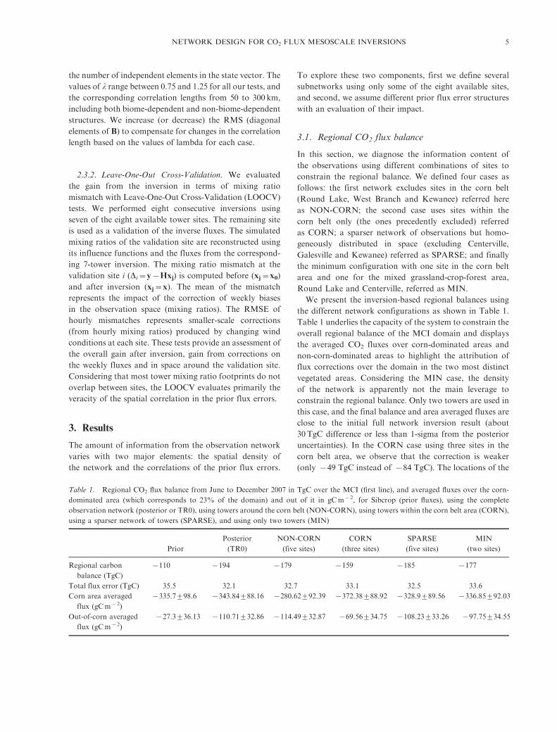
We present the inversion-based regional balances using

the different network configurations as shown in Table 1.

Table 1 underlies the capacity of the system to constrain the

overall regional balance of the MCI domain and displays

the averaged CO2 fluxes over corn-dominated areas and

non-corn-dominated areas to highlight the attribution of

flux corrections over the domain in the two most distinct

vegetated areas. Considering the MIN case, the density

of the network is apparently not the main leverage to

constrain the regional balance. Only two towers are used in

this case, and the final balance and area averaged fluxes are

close to the initial full network inversion result (about

30TgC difference or less than 1-sigma from the posterior

uncertainties). In the CORN case using three sites in the

corn belt area, we observe that the correction is weaker

(only �49 TgC instead of �84 TgC). The locations of the

Table 1. Regional CO2 flux balance from June to December 2007 in TgC over the MCI (first line), and averaged fluxes over the corn-

dominated area (which corresponds to 23% of the domain) and out of it in gCm�2, for Sibcrop (prior fluxes), using the complete

observation network (posterior or TR0), using towers around the corn belt (NON-CORN), using towers within the corn belt area (CORN),

using a sparser network of towers (SPARSE), and using only two towers (MIN)

Prior

Posterior

(TR0)

NON-CORN

(five sites)

CORN

(three sites)

SPARSE

(five sites)

MIN

(two sites)

Regional carbon

balance (TgC)

�110 �194 �179 �159 �185 �177

Total flux error (TgC) 35.5 32.1 32.7 33.1 32.5 33.6

Corn area averaged

flux (gCm�2)

�335.7998.6 �343.84988.16 �280.62992.39 �372.38988.92 �328.9989.56 �336.85992.03

Out-of-corn averaged

flux (gCm�2)

�27.3936.13 �110.71932.86 �114.49932.87 �69.56934.75 �108.23933.26 �97.75934.55

NETWORK DESIGN FOR CO2 FLUX MESOSCALE INVERSIONS 5

towers seem more important than the absolute number of

sites. Considering the averaged fluxes over corn-dominated

areas and grass-dominated areas, the complete network

case (referred here as posterior) indicates a slight increase

of the uptake in corn-dominated areas and an important

increase elsewhere (cf. Table 1). The posterior uncertainties

over the domain for the different cases vary from 5 to

10% error reduction compared to the initial uncertainties.

A large fraction of the domain being unconstrained by

the observations, the error reduction is relatively small

for the different cases. Although most cases as can be seen

in Table 1 show similar flux corrections for the corn area

(between the prior and posterior values), the NON-CORN

case shows here an opposite flux correction in the corn area

due to the absence of observation sites. We investigate the

spatial distribution of the corrections in the next section.

3.2. Spatial flux distributions

The spatial distribution of the corrections appears criti-

cal around the central Corn Belt, and the net fluxes

averaged over the corn area remains similar (Table 1).

The initial spatial distribution (prior flux) was centred

and highly correlated with the corn-dominated area

[Fig. 1(a)]. In the posterior fluxes, the sink area is extended

to the South (northern Missouri) and to the North�

West and North�East (South Dakota and Wisconsin)

[cf. Fig. 1(b)].

With the inversion including only corn sites [Fig. 1(d)],

the averaged fluxes in the non-corn-dominated areas show

the smallest increase in uptake. The uptake in the north-

eastern part of the domain remains low [case CORN and

MIN, or (d) and (f) in Fig. 1]. In the other cases, both

Galesville and LEF towers introduce an increase of

the uptake [NON-CORN and SPARSE, or (c) and (e) in

Fig. 1], i.e. extending the sink area to the North East. The

most variable and important change compared to the initial

setup occurs in northern Illinois where there is the largest

uptake in the posterior fluxes [Fig. 1(b)]. Comparatively,

the prior fluxes showed a maximum around Round Lake

in northern Iowa and southern Minnesota [Fig. 1(a)].

The maximum in Illinois is present only if the Kewanee

or West Branch sites are included [CORN and SPARSE, or

(d) and (e) in Fig. 1]. Other cases produce the maximum of

uptake in northern Iowa and southern Minnesota (MIN),

or decrease the uptake but without detecting the northern

Illinois area (NON-CORN). The tower sites at Centerville

or Galesville are located about 300 km from northern

Illinois but do not produce an increase in uptake.

3.3. Spatial distribution of flux corrections

We present the flux corrections shown in Fig. 2 to highlight

the contribution of different combination of towers applied

to the prior fluxes. Across the four cases, the main spatial

patterns are conserved indicating consistent corrections

across towers. The only case which indicates a disagree-

ment between tower corrections is NON-CORN, with an

important positive correction around Round Lake. The

presence of Round Lake in the other cases induces little to

no change around the tower location. Overall, the intensity

of these changes is highly variable. In most cases, the large

uptake around Round Lake is decreased, the NON-CORN

case being the most positive correction in this area. Once

again, the corrections appear only when towers are in

the area of interests (e.g. the negative correction around

Centerville in NON-CORN and MIN) or when two towers

surround the area (Ozarks and WBI also decrease the

Centerville area in SPARSE). The positive correction

around Round Lake is produced in all cases. Otherwise,

the corrections disappear if the closest tower is missing. As

an illustration of the prior error correlation impact on the

retrieved fluxes, the Fig. 2(b) shows the flux corrections if

biome-related structures are removed from the prior errors.

We will discuss this point in Section 4.

3.4. Theoretical error reduction and observed flux

corrections

We now consider an experimental network design based on

the error reduction only. We compare here the theoretical

benefits from our system (without using observations) to

the actual changes in the posterior fluxes (with observa-

tions). Because the two are basically related to the prior

flux error structures, we investigate the impact of different

correlation structures on the flux corrections and the error

reduction. The impact of the prior fluxes themselves was

investigated in the study of Lauvaux et al. (2012).

The reference setup TR0 includes all the towers in the

region and flux error covariances based on ecosystems and

distance (L�300 km). The error covariances are based on

model-data mismatch and correlation analysis using several

eddy-flux sites over the domain (Lauvaux et al., 2012). As a

comparison, for a similar correlation length but without

considering ecosystems, the overall constraint in our system

is equivalent to L�100 km. The biome dependence, as

defined here, reduces the initial correlation length (cf. Fig.

3). We then ran our 7-month inversion at the weekly time

scale. The error reduction in Fig. 3(a) is about 30�40% in

the vicinity of the towers and about 10�20% in the first

100�200 km. We then ran a second inversion (case TRD)

6 T. LAUVAUX ET AL.

(a) TR0: Complete network of towers (b) TRD: Complete networkof towers

with L = f (distance) (no biome dependence)

(c) NON-CORN: no Corn Belt sites (d) CORN: Corn Belt sites only

(e) SPARSE: Sparser network (f) MIN: Minimal network

Fig. 2. CO2 flux correction from June to December in TgC.degree�2 over the MCI using the SiBcrop prior fluxes, with our reference

case, i.e. the inverse system using the entire network of observation sites (a), with the entire network but the flux error correlation is built on

an exponentially decreasing model only (b), using only the sites out of the Corn Belt area (c), using the sites only within the Corn Belt area

(d), using a sparser network (e) and using a minimal configuration of two sites (one in the Corn Belt and one out) (f).

NETWORK DESIGN FOR CO2 FLUX MESOSCALE INVERSIONS 7

using the same standard deviations for every 20 km by

20 km pixels, but prior flux error correlations are based

on the distance only, with an exponentially decaying model

(L�300 km). The simpler structure of the prior flux errors

here induces the propagation of corrections in space from

grass to corn dominated pixels for example. This assump-

tion seems somewhat unrealistic as Net Ecosystem Ex-

change (NEE) for corn is driven by a different phenology

and several human-driven processes such as irrigation or

fertilisation. Corrections applied to corn-dominated pixels

might not be applicable to grassland areas as vegetation

responses and error sources might be highly variable across

these ecosystems. The spatial distribution of the error

reduction [Fig. 3(a) and (b)] for the two cases shows large

differences. The second case (TRD) shows exponentially

decreasing error reduction from the tower locations as

prescribed by the error correlations.

The flux corrections from these two cases [cf. Fig. 2(a)

and (b)] show clear differences even though their respective

regional carbon balances remain close, with �194 TgC for

the TR0 case and �179 TgC for the TRD case. Posterior

uncertainties and fluxes are highly affected by the assump-

tions in the prior error statistics even if the main patterns

remain somehow similar. The posterior flux errors for

the TR0 case are about 32TgC (with 35.5TgC error in the

prior fluxes), whereas the TRD case posterior errors are

about 25.2 TgC (with an error of 30.5 TgC in the prior

fluxes). The relationship between prior error structures and

posterior errors and fluxes has a consequent impact on the

flux errors, but little impact on the regional carbon balance

(posterior fluxes). In Section 4, we investigate the observa-

tional constraint and the validity of the flux error correla-

tion assumption by estimating the degree of freedom of

the signals (DFS) (Rodgers, 2000; Bocquet, 2009) and by

evaluating the flux corrections on towers that were not used

in the inversion from our different cases (LOOCV).

4. Discussion

4.1. Optimal choice of prior error structures

The different inversions performed here and their inter-

pretation are highly dependent on the prior error covar-

iances. Wu et al. (2011) noted the impact of incorrect flux

error correlations in the prior error covariance matrix.

The definition of prior error structures in space remains

difficult to estimate quantitatively, and several studies

discussed the estimation of the potential correlations using

different techniques. Although geostatistical approaches

propose to diagnose these structures from different ob-

servational datasets (Michalak et al., 2005), other inverse

studies have optimised these distances based on correlation

analysis of biogeochemical models (Rodenbeck et al., 2003;

Chevallier et al., 2006) or derived them from climatological

and ecological considerations (Peters et al., 2007). At large

scale, the ill-conditioning of the inverse problem leads to

significantly long spatial flux error correlations in order to

keep a sufficient observational constraint. Here, a large

(a) TR0: Complete network of towers (b) TRD: Complete networkof towers

with L = f (distance) (no biome dependence)

Fig. 3. Error reduction in % using all the towers and prior flux errors with ecosystem-based standard deviations (RMS) and spatial

correlations based on ecosystems and distances between pixels (case TR0) (a) and the second case considering correlations with distance

only (exponentially decaying model) (TRD) (b).

8 T. LAUVAUX ET AL.

number of observations and the relatively short distances

between sites tend to rapidly reduce the DFS and lead to

the convergence of the solutions. The estimation of flux

error correlations, if they exist, is required to obtain precise

estimates of the a posteriori flux errors. We performed

several tests using only a subsample of the complete net-

work, with several observation sites available for a cross-

validation of the corrections. We considered here the

case CORN, using only Round Lake, West Branch and

Kewanee sites, the other five being used as independent

observations to evaluate the flux corrections. We define

three cases with different correlation structures, the first

one using a correlation length of 300 km, exponentially

decaying with the distance, and combined with the biome

map of the region (Lauvaux et al., 2012) (referred here as

TR0), then a second case using correlation length of 300

km only (TRD) and finally a third case with a correlation

length of 50 km (L50). We estimated the gain in terms of

the final CO2 concentration mismatch compared to the

initial (a priori) model-data mismatch at the five remaining

towers, in ppm. Over the 28 periods of inversions from

June to December, the gain for the cases TR0 or TRD

improves the initial mismatch by 0.823 and 0.861 ppm,

respectively, compared to the case L50 with only 0.561 ppm.

On average, the simpler exponentially decaying model

(�TRD) shows a larger gain compared to the more

complex vegetation-based description TR0, but 4 of the

28 periods show small net degradations of the initial

mismatch, against two for the TR0 case. Similarly, the

DFS drops from 284 for the case L50, and 281 for the TR0

case, down to 59 for the case TRD, indicating an important

increase of the apparent observational constraint due to the

correlation length in the flux errors. This first analysis

shows that the larger flux correlations of 300 km seems the

most profitable assumption in terms of gain. But the

presence of degradation of several periods (4 out of 28)

indicates that more refinement is required, including

temporal variability for example. The gain increasing

with the correlation length might also correspond to the

overall decrease of the regional flux bias. This overall gain

remains valid at the regional scale, but the inherited

structures in space in the posterior fluxes might be artificial,

constrained by the assumed correlation length more than

the data and their adjoint transport.

4.2. Cross-validation of posterior fluxes

We performed LOOCVs to evaluate the gain at each tower

in terms of the CO2 concentration mismatch. The principle

of cross-validation relies on eight inversions using seven

towers only out of the eight available concentration sites.

The retrieved fluxes are then propagated through the

influence function of the validation tower. The improve-

ment in the concentration mismatch at the eliminated tower

is a direct evaluation of the posterior fluxes. We computed

both RMSEs and means for each of the inversions with a

different validation tower. This analysis evaluates the

assumptions made in the prior flux errors (spatial correla-

tion) in terms of systematic error corrections and sub-

weekly corrections (RMSE). The results are presented in

Table 2. The means show that all the inversions, but one

provides smaller mismatch at the validation tower. We

conclude here that the inversion improved the fluxes in

terms of systematic errors at the weekly timescale. In terms

of RMSE, the results indicate no or little decrease in

the concentration mismatch compared to the reference

inversion (using the eight concentration towers), with an

increase of the mismatch in three cases. The absence of

Table 2. Mixing ratio residuals in ppm for each tower, averaged over the 7 months (mean) and their related RMSE at the hourly time

scale before and after inversion. The three lines correspond to the initial mismatch between modelled and observed mixing ratios (a priori),

posterior residuals after inversion using the eight towers (a posteriori) and residuals from each inversion excluding the tower indicated in

the first line, used for validation (LOOCV)

Centerville Kewanee Round Lake Mead Galesville Missouri WBI LEF

A priori

Mean �1.708 �1.248 �0.583 �1.025 �1.912 �0.578 �1.203 �0.167

RMSE 7.641 7.169 7.284 6.858 7.970 7.884 8.341 6.786

A posteriori

Mean �0.103 �0.028 �0.104 �0.074 �0.162 0.102 0.467 0.171

RMSE 3.711 3.757 3.638 3.511 4.244 4.067 4.269 3.837

LOOCV

Mean �1.045 �0.283 �0.613 �0.883 �1.371 �0.119 0.235 0.865

RMSE 7.003 7.564 7.479 6.794 7.602 7.727 7.656 7.848

Residuals in LOOCV correspond to cross-validation of the inverse fluxes retrieved from the Leave-One-Out experiments. Values closer to

zero compared with the a priori mismatch indicate an improvement.

NETWORK DESIGN FOR CO2 FLUX MESOSCALE INVERSIONS 9

improvement in the RMSE shows that the subweekly

variability due to smaller-scale flux signals is not captured

correctly compared to the reference inversion. The spatial

error correlation might be over-estimated in our setup,

even though the regional balance with fewer towers is

consistent with previous findings. The small structures

in the flux corrections are not realistic at the validation

tower. The extent of corrections in space is artificial

and only helps to improve larger-scale systematic errors.

However, the two inversions without WBI or Kewanee

show almost identical improvements compared to the

reference inversion in terms of means of the mismatch.

The redundancy of the information from these two towers

is in agreement with earlier findings, co-located in the corn

belt area.

4.3. Estimation of prior error structures

From our analysis, we can disaggregate two correction

terms from the flux correction, one due to local atmo-

spheric signals, and one induced by the presence of spatial

correlations in the prior flux errors. The second seems

consistent following our previous tests. Even if not perfect,

long correlation lengths (L�300 km) showed an improve-

ment compared to the initial CO2 concentration mismatch,

and better results than smaller correlation lengths (L�50

km). For the first term, the simulated atmospheric mixing

drives primarily the size of the main area of influence on

the concentrations. The model resolution might affect the

dimensions of the concentration footprints noting that

horizontal diffusion is related to model parameterisation

optimised at given resolutions. Comparisons are needed to

explore the sensitivity of the footprint size to the model

configuration. Although the two terms might seem contra-

dictory, they reflect two different facts. The first term

represents directly observed flux signals in the atmospheric

concentrations. The second term represents the common

sources of errors in the fluxes. This term is problematic in

the sense that corrections are distributed spatially, even

though the observations alone were not able to constrain

these areas initially. Chevallier et al. (2006) investigated

the presence of flux error correlations using eddy-flux

sites, at a daily time scale. The temporal scale of this study

was shorter than the present pixel-based inversion at the

weekly time scale. They found no clear spatial structures

in the prior flux errors. Hilton (2011) optimised parameters

of a vegetation model with 100 eddy-covariance NEE

measurement sites across North America and diagnosed

the covariances in the residuals. The most likely correlation

length was about 400 km at the monthly time scale and

200 km at the 10-day time scale. Before that, Rodenbeck

et al. (2003) performed model sensitivity tests at the

monthly time scale and diagnosed correlation lengths of

about 1200 km. Michalak et al. (2005) proposed the use

of the Maximum Likelihood algorithm to derive prior flux

error correlations based upon observations which were

a direct result of those fluxes. While the method is very

informative for the modellers to evaluate the balance

of the inverse system, the reality of flux error correlations

has to be investigated, not only to fit the inverse setup

because of other limiting factors (model resolution,

number of observations, dimension of the matrices to

invert), but also to represent the real structures of the prior

flux errors.

5. Conclusions

We have evaluated here the CO2 posterior fluxes over

the corn belt of the US Midwest by subsampling the

MCI tower network. Atmospheric inversions at 20-km

resolution were performed for a 7-month period, with

similar assumptions but variable observational con-

straints. These sensitivity tests correspond to different net-

work configuration, including a sparser network of

observations or ecosystem-specific networks. The four

different subsampled networks showed consistent regional

carbon balances despite tower removals (�178 TgC9 13).

The DFS showed that the posterior fluxes are constrained

mainly by flux error correlation when the correlation length

is larger than 150 km. The gain in the final concentration

mismatch indicates an improvement of the overall regional

fluxes with large correlation length (300 km or more) but

might correspond to artificial extension of the regional

bias correction rather than realistic spatial structures in

the posterior fluxes. This preliminary study shows that

the MCI campaign provides a sufficient number of obser-

vations to constrain the Corn Belt carbon balance over

the 7-month period, but the spatial distribution of the

inverse fluxes is still under-constrained with too little obser-

vational constraint compared to the assumed flux error

structures.

6. Acknowledgements

We thank Arlyn Andrews from NOAA/ESRL for provid-

ing the data from the West Branch tall tower site (WBI)

and the WLEF tower (LEF). We thank Peter J. Rayner for

fruitful discussions. This work was supported by the Office

of Science (BER) US Department of Energy, Terrestrial

Carbon Program, the US National Aeronautics and Space

Administration’s Terrestrial Ecology Program, the US

National Oceanographic and Atmospheric Administration,

Office of Global Programs and Global Carbon Cycle

Program.

10 T. LAUVAUX ET AL.

References

Bocquet, M. 2009. Towards optimal choices of control space

representation for geophysical data assimilation. Mon. Weather

Rev. 137, 2331�2348. Online at: http://journals.ametsoc.org/doi/

abs/10.1175/2009MWR2789.1

Canadell, J. G., Le Quere, C., Raupach, M. R., Field, C. B.,

Buitenhuis, E. T. and co-authors. 2007. Contributions to

accelerating atmospheric CO2 growth from economic activity,

carbon intensity, and efficiency of natural sinks. Proc. Natl Acad.

Sci. 104(47), 18866�18870. DOI: 10.1073/pnas.0702737104. On-

line at: http://www.pnas.org/content/104/47/18866.abstract

Chevallier, F., Viovy, N., Reichstein, M. and Ciais, P. 2006. On

the assignment of prior errors in Bayesian inversions of CO2

surface fluxes. Geophys. Res. Lett. 33, L13802. DOI: 10.1029/

2006GL026496. Online at: http://www.agu.org/pubs/crossref/

2006/2006GL026496.shtml

Ciais, P., Rayner, P., Chevallier, F., Bousquet, P., Logan, M.

and co-authors. 2010. Atmospheric inversions for estimating

CO2 fluxes: methods and perspectives. Clim. Change 103(1/2),

69�92. DOI: 10.1007/s10584-010-9909-3. Online at: http://www.

springerlink.com/content/pnk685jh102375r0/

Gerbig, C., Dolman, A. J. and Heimann, M. 2009. On observa-

tional and modelling strategies targeted at regional carbon

exchange over continents.Biogeosciences 6(10), 1949�1956. DOI:

10.5194/bg-6-1949-2009. Online at: http://www.biogeosciences.

net/6/1949/2009/

Gerbig, C., Lin, J. C., Munger, J. W. and Wofsy, S. C. 2006. What

can tracer observations in the continental boundary layer tell

us about surface-atmosphere fluxes? Atmos. Chem. Phys. 6(2),

539�554. DOI: 10.5194/acp-6-539-2006. Online at: http://www.

atmos-chem-phys.net/6/539/2006/acp-6-539-2006.html

Gloor, M., Bakwin, P., Hurst, D., Lock, L., Draxler, R. and

co-authors. 2001. What is the concentration footprint of a tall

tower? J. Geophys. Res. 106, 17831�17840.

Gockede, M., Michalak, A. M., Vickers, D., Turner, D. P. and

Law, B. E. 2010a. Atmospheric inverse modeling to constrain

regional scale CO2 budgets at high spatial and temporal

resolution. J. Geophys. Res. 115, D15113. DOI: 10.1029/

2009JD012257. Online at: http://www.agu.org/pubs/crossref/

2010/2009JD012257.shtml

Gockede, M., Turner, D. P., Michalak, A. M., Vickers, D. and

Law, B. E. 2010b. Sensitivity of a subregional scale atmospheric

inverse CO2 modeling framework to boundary conditions.

J. Geophys. Res. 115, D24112. DOI: 10.1029/2010JD014443.

Online at: http://www.agu.org/pubs/crossref/2010/2010JD014443.

shtml

Gurney, K. R., Mendoza, D., Zhou, Y., Fischer, M., Miller, C.

and co-authors. 2009. High resolution fossil fuel combustion

CO2 emission fluxes for the United States. Environ. Sci. Technol.

43(14), 5535�5541. Online at: http://pubs.acs.org/doi/abs/10.

1021/es900806c

Hilton, T. W. 2011. Spatial Structure in North American

Terrestrial Biological Carbon Fluxes and Model Errors Evaluated

with a Simple Land Surface Model. PhD Dissertation. The

Pennsylvania State University. Online at: http://etda.libraries.

psu.edu/

Keenan, T. F., Baker, I., Barr, A., Ciais, P., Davis, K. and

co-authors. 2012. Terrestrial biosphere model performance for

inter-annual variability of land-atmosphere CO2 exchange.

Glob. Change Biol. 18(6), 1971�1987. DOI: 10.1111/j.1365-2486.

2012.02678.x.

Knorr, W. and Heimann, M. 2001. Uncertainties in global

terrestrial biosphere modeling, part II: global constraints for a

process-based vegetation model. Glob. Biogeochem. Cycl. 15,

227�246. Online at: http://www.agu.org/pubs/crossref/2001/

1998GB001060.shtml

Lauvaux, T., Gioli, B., Sarrat, C., Rayner, P. J., Ciais, P. and

co-authors. 2009. Bridging the gap between atmospheric con-

centrations and local ecosystem measurements. Geophys. Res.

Lett. 36, L19809. DOI: 10.1029/2009GL039574. Online at:

http://www.agu.org/pubs/crossref/2009/2009GL039574.shtml

Lauvaux, T., Schuh, A. E., Uliasz, M., Richardson, S., Miles, N.

and co-authors. 2012. Constraining the CO2 budget balance of

the corn belt: exploring uncertainties from the assumptions in

a mesoscale inverse system. Atmos. Chem. Phys. 12, 337�354.

DOI: 10.5194/acp-12-337-2012. Online at: http://www.atmos-

chem-phys.net/12/337/2012/acp-12-337-2012.html

Lauvaux, T., Uliasz, M., Sarrat, C., Chevallier, F., Bousquet, P.

and co-authors. 2008. Mesoscale inversion: first results from the

Ceres campaign with synthetic data. Atmos. Chem. Phys. 8(13),

3459�3471. DOI: 10.5194/acp-8-3459-2008. Online at: http://

www.atmos-chem-phys.net/8/3459/2008/

LeQuere, C., Raupack, M. R., Canadell, J., Marland, G., Bopp, L.

and co-authors. 2009. Trends in the sources and sinks of carbon

dioxide. Nat. Geosci. 2, 831�836. DOI: 10.1038/ngeo689. Online

at: http://www.nature.com/ngeo/journal/v2/n12/abs/ngeo689.html

Lokupitiya, E., Denning, S., Paustian, K., Baker, I., Schaefer, K.

and co-authors. 2009. Incorporation of crop phenology in

Simple Biosphere Model (SiBcrop) to improve land-atmosphere

carbon exchanges from croplands. Biogeosciences 6, 969�

986. DOI: 10.5194/bg-6-969-2009. Online at: http://www.

biogeosciences.net/6/969/2009/

Michalak, A. M., Hirsch, A., Bruhwiler, L., Gurney, K. R.,

Peters, W. and co-authors. 2005. Maximum likelihood estima-

tion of covariance parameters for Bayesian atmospheric trace

gas surface flux inversions. J. Geophys. Res. 110, D24107. DOI:

10.1029/2005JD005970. Online at: http://www.agu.org/pubs/

crossref/2005/2005JD005970.shtml

Miles, N. L., Richardson, S. J., Davis, K. J., Lauvaux, T.,

Andrews, A. E. and co-authors. 2012. Large amplitude spatial

and temporal gradients in atmospheric boundary layer CO2

mole fractions detected with a tower-based network in the U.S.

upper midwest. J. Geophys. Res. 117(B), G01019. DOI: 10.1029/

2011JG001781. Online at: http://www.agu.org/pubs/crossref/

2012/2011JG001781.shtml

Ogle, S., Breidt, F., Easter, M., William, S., Killian, K. and

Paustian, K. 2010. Scale and uncertainty in modeled soil organic

carbon stock changes for us croplands using a process-based

model. Glob. Change Biol. 16, 810�822. DOI: 10.111/j.1365-

2486.2009.01951.x. Online at: http://onlinelibrary.wiley.com/

doi/10.1111/j.1365-2486.2009.01951.x/abstract

Peters, W., Jacobson, A. R., Sweeney, C., Andrews, A. E.,

Conway, T. J. and co-authors. 2007. An atmospheric perspective

NETWORK DESIGN FOR CO2 FLUX MESOSCALE INVERSIONS 11

on North American carbon dioxide exchange: CarbonTracker.

Proc. Natl Acad. Sci. 104(48), 18925�18930. DOI: 10.1073/

pnas.0708986104. Online at: http://www.pnas.org/content/104/

48/18925.abstract

Raupach, M. R., LeQuere, C. and Heimann, M. 2008. Anthro-

pogenic and biophysical contributions to increasing atmospheric

co2 growth rate and airborne fraction. Biogeosciences 5, 1601�

1613. DOI: 10.5194/bg-5-1601-2008. Online at: http://www.

biogeosciences.net/5/1601/2008/bg-5-1601-2008.html

Ricciuto, D., King, A., Dragoni, D. and Post, W. 2011. Parameter

and prediction uncertainty in an optimized terrestrial carbon

cycle model: effects of constraining variables and data record

length. J. Geophys. Res. 116, G01033. Online at: http://www.

agu.org/pubs/crossref/2011/2010JG001400.shtml

Rodenbeck, C., Houweling, S., Gloor, M. and Heimann, M. 2003.

Time-dependent atmospheric CO2 inversions based on inter-

annually varying tracer transport. Tellus B 55(2), 488�497.

Rodgers, C. D. 2000. Inverse Methods for Atmospheric Sounding:

Theory and Practice. World Scientific, Singapore.

Schuh, A. E., Denning, A. S., Corbin, K. D., Baker, I. T., Uliasz,

M. and co-authors. 2010. A regional high-resolution carbon

flux inversion of North America for 2004. Biogeosciences 7(5),

1625�1644. DOI: 10.5194/bg-7-1625-2010. Online at: http://

www.biogeosciences.net/7/1625/2010/

Schwalm, C. R., Williams, W. A., Schaefer, K., Anderson, R.,

Arain, M. A. and co-authors. 2010. A model-data intercompar-

ison of CO2 exchange across North America: results from the

North American carbon program site synthesis. J. Geophys. Res.

115, G00H05. DOI: 10.1029/2009JG001229. Online at: http://

www.agu.org/pubs/crossref/2010/2009JG001229.shtml

Uliasz, M. 1994. Lagrangian particle modeling in mesoscale

applications. In: Environmental Modelling II (ed. P. Zanetti).

Computational Mechanics Publications, Southampton, pp.

71�102.

Wang, Y. P., Leuning, R., Cleugh, H. and Coppin, P. A. 2001.

Parameter estimation in surface exchange models using non-

linear inversion: how many parameters can we estimate and

which measurements are most useful? Glob. Change Biol. 7,

495�510. Online at: http://onlinelibrary.wiley.com/doi/10.1046/

j.1365-2486.2001.00434.x/abstract

West, T. O., Bandaru, V., Brandt, C. C., Schuh, A. E. and Ogle,

S. M. 2011. Regional uptake and release of crop carbon in the

United States. Biogeosciences 8, 631�654. Online at: http://www.

biogeosciences.net/8/2037/2011/bg-8-2037-2011.html

Wu, L., Bocquet, M., Lauvaux, T., Chevallier, F., Rayner, P. and

Davis, K. 2011. Optimal representation of source-sink fluxes

for mesoscale carbon dioxide inversion with synthetic data.

J. Geophys. Res. 116, D21304. Online at: http://www.agu.org/

pubs/crossref/2011/2011JD016198.shtml

12 T. LAUVAUX ET AL.