Network delay tomography using ï¬‚exicast experiments

Royal Statistical Society

J. R. Statist. Soc. B (2006)68, Part 5, pp. 785–813

Network delay tomography using flexicastexperiments

Earl Lawrence

Los Alamos National Laboratory, USA

and George Michailidis and Vijayan N. Nair

University of Michigan, Ann Arbor, USA

[Received May 2005. Revised July 2006]

Summary. Estimating and monitoring the quality of service of computer and communicationsnetworks is a problem of considerable interest.The paper focuses on estimating link level delaydistributions from end-to-end path level data collected by using active probing experiments.Thisis an interesting large scale statistical inverse (deconvolution) problem. We describe a flexibleclass of probing experiments (‘flexicast’) for data collection and develop conditions under whichthe link level delay distributions are identifiable. Maximum likelihood estimation using the EMalgorithm is studied. It does not scale well for large trees, so a faster algorithm based on solvingfor local maximum likehood estimators and combining their information is proposed. The use-fulness of the methods is illustrated on real voice over Internet protocol data that were collectedfrom the University of North Carolina campus network.

Keywords: Deconvolution; EM algorithm; Internet; Inverse problem; Tree-structured graphs

1. Introduction

Computer and communications networks form the back-bone of our information society. Overthe last decade, these networks have experienced an exponential growth in terms of the numberof users, the amount of traffic and the complexity of applications. It is important for networkengineers and Internet service providers to be able to estimate and monitor the quality-of-serviceparameters such as link delays, dropped packet rates and available bandwidth. However, thedecentralized nature of modern computer and communications networks has made it difficultto assess performance. Traditional methods based on queuing analysis focus on the behaviourof one or a small number of routers and are inadequate in characterizing the complexities ofsuch networks. This has led to the emergence of network tomography—an area that uses activeand passive traffic measurement schemes to quantify the performance and the quality of serviceof networks. A good review of the area and challenges can be found in Castro et al. (2004).

The term network tomography was introduced in Vardi (1996), which dealt with the esti-mation of origin–destination traffic intensities based on the total measured intensities alongindividual links. See Tebaldi and West (1998), Cao et al. (2000) and Zhang et al. (2003) forrelated work on this problem. Active tomography deals with estimating link level characteris-tics, such as loss rates and delay distributions, by actively probing the network. This involvessending probe packets from one or more sender nodes to a set of receiver nodes and measuring

Address for correspondence: Earl Lawrence, Los Alamos National Laboratory, PO Box 1663, Los Alamos,NM 87545, USA.E-mail: [email protected]

786 E. Lawrence, G. Michailidis and V. N. Nair

the end-to-end characteristics. The goal then is to estimate (‘recover’) the link level informationfrom the end-to-end path level data. This paper focuses on delay distributions.

As an example, consider the emerging application of Internet or ‘voice over Internet proto-col’ (VOIP) telephony. VOIP is a technology that turns voice signals into packets and transmitsthem over the Internet to the intended receivers. The main difference from classical telephony isthat the call does not use a dedicated connection with reserved bandwidth, but instead packetscarrying the voice data are multiplexed in the network with other traffic. For this application,the quality-of-service requirements in terms of packet losses and delays are significantly morestringent than non-realtime applications such as electronic mail. Recently, the University ofNorth Carolina (UNC) entered the planning phase of deploying VOIP telephony and wantedto assess its campus network to determine whether it is capable of supporting the technology.To do this, monitoring equipment and software that were capable of placing such phone callswere installed throughout the campus network. The software allows the emulation of VOIPcalls between the monitoring devices. It then synchronizes the clocks and obtains very accuratepacket loss and delay measurements along the network paths.

15 monitoring devices from Avaya Laboratories were deployed in a variety of buildings andon a range of capacity links through the UNC network. The locations included dormitories,libraries and various academic buildings. The links included large capacity gigabit links, smaller100 Mbit links and one wireless link. Monitoring VOIP transmissions between these buildingsallows us to examine traffic influenced by the physical conditions of the link and the demandsof various groups of users. Fig. 1(a) gives the physical connectivity of the UNC network. Eachof the nodes on the circle has a basic machine that can place a VOIP phone call to any ofthe other end points. The three nodes in the middle are part of the core (main routers) of thenetwork. One of these internal nodes, the upper router linked to Sitterson Hall, also connectsto the gateway that exchanges traffic with the rest of the Internet. The measured data consist ofend-to-end delays and losses. We shall use data that were collected from this study to illustrateour methodology in Section 8.

Although the physical structure of a network can be arbitrary (Fig. 1(a)), the logical topologyfor the probing experiment can be represented more simply (Fig. 1(b)). We shall follow the com-mon practice in the literature and focus attention on logical topologies that can be described bytrees: acyclic graphs with one vertex designated as the root (Fig. 2(b)). Formally, let T = .V , E/ bea tree with node set V and link set E . The nodes follow a canonical numbering scheme, startingfrom the root node 0. All links will be named after the node at their terminus so, in Fig. 2, link

Fig. 1. (a) Schematic diagram of the UNC network and (b) logical topology of the network

Network Delay Tomography 787

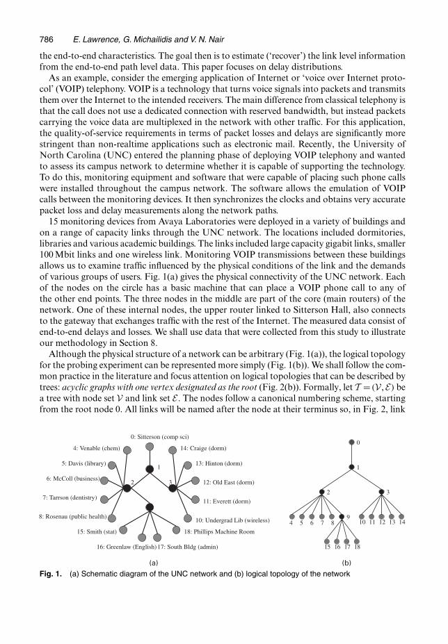
Fig. 2. (a) Three-layer, binary, symmetric tree and (b) general tree with notation

1 refers to the link connecting nodes 0 and 1. The parent of node k ∈V will be written f.k/.In a tree, all nodes have a parent except for the root node. Define f i.k/ recursively as follows:f i.k/ = f{f i−1.k/}, where f 1.k/ = f.k/. Node k is said to be in layer L if f L.k/ = 0. Let D.k/

denote the children of node k, which is the collection of nodes whose parent is k. Let R denotethe set of leaf or receiver nodes, i.e. nodes with no children. Finally, an internal node is a nodewith both a parent and a set of children. Fig. 2(a) shows a simple binary tree with three layers.We shall use it later to illustrate some of the techniques.

Packets can be sent from a source to a destination by using two basic transmission protocols:a ‘unicast’ scheme that sends a packet from a source to one receiver at a time, and a ‘multicast’scheme that sends a packet simultaneously to a set of specified receivers. In previous work, theterm multicast experiment refers to the situation in which all the receiver nodes are probedsimultaneously. We shall refer to it instead as an ‘omnicast’ probing experiment. The ‘flexicast’experiments in Section 3 are also based on multicast transmission, although they do not involvesending the packet to all receivers in the network.

The estimation of loss rates based on active probing has been studied by many researchers(see Cáceres et al. (1999), Xi et al. (2007) and references therein). Link delay tomography wasfirst studied by Lo Presti et al. (2002), who developed a heuristic estimator for omnicast exper-iments based on solving polynomial equations, which can be very inefficient. Liang and Yu(2003) developed a pseudolikelihood approach by considering all possible pairwise results fromeach individual full omnicast result. We shall compare these two techniques with our methodslater in the paper. Shih and Hero (2003) presented an estimator that models link delay by usinga point mass at zero and a finite mixture of Gaussian distributions.

The rest of the paper is organized as follows. Section 2 describes the models and assumptions.Section 3 describes the framework for probing studies, introduces flexicast probing experi-ments and studies conditions under which the link level delay parameters are estimable from


end-to-end, path level data. Section 4 deals with maximum likelihood estimation using the EMalgorithm and develops its computational and theoretical aspects. Alternative heuristic algo-rithms that are faster and scale well to larger networks are discussed in Section 5. An extensivenumerical investigation of the procedures is also presented by using the ns-2 network simu-lation software. Finally, the methods are illustrated on real data that were collected from theUNC campus network.

2. Models and assumptions

Following Lo Presti et al. (2002) and Liang and Yu (2003), we shall consider nonparamet-ric estimation of the delay distributions by using a discrete distribution with a fixed, univer-sal bin size. Specifically, let Xk be the delay that is accumulated on link k, taking values inthe set {0, q, . . . , bq}. Here q is the bin size and b is the maximum discrete delay (which isassumed to be common for all the links). Although this framework seems restrictive, it is use-ful for several reasons. First, experience with real network traffic data shows that behaviourtends to vary with the particular network being studied, so selecting a particular parametricfamily for modelling the link delay distribution is difficult. Moreover, the delay data typicallyexhibit bursty behaviour, in which case the tails of the distribution are of considerable inter-est. The discrete model makes no assumptions about where the mass is located, so the tailsof heavy-tailed distributions can be estimated provided that we have a sufficient number ofprobes. The bin size can be chosen adaptively after the data have been collected. Smaller binsizes can be used to estimate detailed information about the distribution. Large bin sizes canbe used to obtain tail information. Examples of this will be discussed in the data analysissection.

Throughout the paper, we shall ignore losses or infinite delays. We can always estimate theloss rates and the finite delay distributions separately and combine the results to estimate theoverall network behaviour. In addition, we make the assumption (which is common in the net-work tomography literature) that the packet delays are temporally independent and that thedelay of a packet on a link is independent of the delay on the other links in the path. Theassumption of temporal independence is reasonable as long as the interval between probes issufficiently large. Temporal stationarity is reasonable as long as the probing period is sufficientlyshort to avoid major network changes. The adequacy of the spatial assumption will depend onthe particular network being studied and whether there are other physical links connecting thenodes.

The data are collected by recording the total delay that a packet experiences as it travels fromthe root node to the receiver nodes. For example, in Fig. 2(b), probe packets would be sent fromnode 0 to various collections of nodes 2, 3, 6, 8, 9, 10, 11, 12, 13, 14 and 15 and the delays thatare experienced along their corresponding paths would be recorded. Physically, each end-to-enddelay is the sum of the individual link delays along the path. If a scheme has a collection of k

receivers, a single observation would be a k-tuple of delays.Let P0,k denote the path from node 0 to node k, and let

Yk = ∑i∈P0,k

Xi

be the cumulative delay accumulated from the root node to node k. For example, Y3 =X1 +X3in Fig. 2(b). The measurements that are obtained from a delay tomography experiment consistof cumulative delays Yr, r ∈R. Let αk.i/=P.Xk = iq/, i=1, . . . , b. Our objective is to estimatethis set of values for k ∈E and i in {0, 1, . . . , b} by using the Yr-measurements.


In what follows, we shall use the notation �αk = .αk.0/, αk.1/, . . . , αk.b//′ and �α = .�α′0,

�α′1, . . . , �α′

|E |]/′. Let πj,k.i/ be the probability that the delay that is accumulated on path Pj,k

is equal to i units. This is a function of �α.

3. Flexicast probing experiments

Although the omnicast probing experiment is easy to implement, it suffers from several disad-vantages. Suppose that there are R receivers and the total number of possible bins associatedwith the path level delay distribution of the ith receiver is Bi. Then, the total number of possibleoutcomes is of order ΠR

i=1Bi, which can be a huge number. As we shall see later, the computa-tional efficiency of most estimation methods depends on this number. As an example, let eachlink level delay distribution have the same number of bins: b=4. Further, suppose that we havea symmetric binary tree with five layers. Then, there are R=16 receivers and Bi =19 for the pathlevel delay distributions of all the receivers, so the approximate number of possible outcomes is2:8×1020.

A second, perhaps more important, issue is the lack of flexibility as it involves probing theentire network each time. In practice, we are interested in monitoring the network over a periodof time, and so we need a flexible scheme that allows us to probe different parts of the networkwith different degrees of intensity depending on where there are bottle-necks or quality-of-service problems. We consider a flexible class of probing experiments called ‘flexicast’ experi-ments to address these problems in the context of delay tomography.

Define a k-cast scheme as a scheme that sends probes from a receiver to a specified set ofk receiver nodes. For example, for the tree in Fig. 2(b), 〈2,3〉 is a two-cast (or bicast) schemewhereas 〈6, 12, 13, 14, 15〉 is a five-cast scheme. A flexicast experiment C is a combination ofk-cast schemes Cj, j =1, . . . , M, with possibly different values of k, that allows us to estimate allthe link level parameters. Returning to Fig. 2, one flexicast experiment made up of a collectionof bicast and unicast schemes is C ={〈2,3〉, 〈6, 12〉, 〈13, 14〉, 〈8, 9〉, 〈10〉, 〈11〉, 〈15〉}. Another thatuses larger k-casts is C ={〈2,3〉, 〈6, 12, 13, 14, 15〉, 〈8, 9, 10, 11〉}.

A natural question is when will a flexicast experiment lead to identifiability? We providebelow a necessary and sufficient condition. The proof is based on the idea that an individualk-cast probe can identify all the path distributions between branching nodes on its subtree. Itsuffices for the collection to be sufficiently rich in terms of subtrees that the individual links canbe expressed as functions of paths from different schemes. We formalize this intuition in thefollowing proposition. The proof is deferred to Appendix A.

Proposition 1. Let T be a general tree network, and suppose that its link delay distributionsare discrete. Let C be a collection of k-cast schemes Cj, j =1, . . . , M. The link level delay distri-butions are identifiable if and only if

(a) for every internal node s∈T \{0, R} there is at least one k-cast scheme Cj ∈C, with k> 1,such that s is a branching node for Cj, and

(b) every receiver r ∈R is covered by at least one Cj ∈C.

Remark 1. We have restricted attention to discrete distributions as they are the focus of thepresent paper, but the result holds more generally. First, the result can be shown to hold as longas the distribution has at least one point mass. It will also hold for purely continuous distribu-tions under some conditions (such as higher order moments depending on the mean). It doesnot, however, hold for arbitrary continuous distributions. This can be seen easily by using atwo-layer tree (the top two layers of the tree in Fig. 2(a)) with a source node 0, internal node 1


and receiver nodes 2 and 3. Let the link level delay random variables be X1, X2 and X3 and thepath level delay random variables at receiver nodes 2 and 3 be Y2 =X1 +X2 and Y3 =X1 +X3.Suppose that the Xis are independent N.μi, 1). Then, we cannot recover the μis from the jointdistribution of Y2 and Y3.

4. Maximum likelihood estimation

Active delay tomography is a large scale inverse problem. For example, consider the omnicastproblem for the topology that is given in Fig. 2(b). Here we must use the 11-dimensional end-to-end measurements to estimate the 15 link delay distributions. The key is the dependenceamong the 11-dimensional data that is induced by the simultaneous probing. This dependencegives us additional information that allows us to deconvolve the path level delay into link levelinformation. We consider maximum likelihood estimation first.

We need some additional notation. Let T Cj be the subtree that is probed by scheme Cj ∈C,with node set VCj and link set ECj . Let X Cj = {0, 1, . . . , b}|ECj | be the set of all possible linkdelay combinations that could arise from this scheme. Each x ∈X Cj is an |ECj |-tuple giving apossible link delay combination. Let the function y.x, T Cj / give the end-to-end delay arisingin scheme Cj from link outcome x ∈ X Cj . Define the set of all possible end-to-end delays asYCj ={y.x, T Cj /|x∈X Cj}. Let γCj

.y/=P.YCj =y/, the probabilities for the end-to-end experi-mental outcomes.

We illustrate this notation by using Fig. 2(b). Suppose that we probe the pair 〈2,3〉. Let b=1so Xk ∈{0, 1}. The link set is E 〈2,3〉 ={1,2,3}. Assume that only a single probe packet is used forthis scheme, and it experiences link delays of 0, 1 and 1 on each link. We then have x= .0, 1, 1/

and y = .1, 1/. The probability of this link delay set is

P{X〈2,3〉 = .0, 1, 1/}=α1.0/ α2.1/ α3.1/:

The probability of this end-to-end outcome is

P{Y 〈2,3〉 = .1, 1/}=α1.0/ α2.1/ α3.1/+α1.1/ α2.0/ α3.1/,

which is the sum of the probabilities for the link outcomes which can give rise to this end-to-endoutcome.

4.1. EM algorithmThe discrete nonparametric distribution framework results in multinomial outcomes for pathlevel data. Specifically, the observations consist of the number of times that we observe eachindividual outcome �y from the set of outcomes YCj for a given scheme. Denote these counts asN

Cj

�y . Consider the likelihood equation

l.�α; Y/= ∑Cj∈C

∑�y∈YCj

NCj

�y log{γCj.�y; �α/}: .1/

This expression is difficult to maximize directly. However, it is a classical example of a missingdata problem: if the counts for the unobserved link delays were known, the maximization wouldbe fairly straightforward as the link outcomes are also simple multinomial experiments. The EMalgorithm is a natural candidate for computing the maximum likelihood estimates in this setting.For distributions in exponential families, we need to impute just the sufficient statistics for eachlink: the counts for the number of times that Xk took on each value.


The E-step can be broken into two parts. Assume that we have some parameter vector�α.q−1/. First, we compute the expected number of times that each link delay vector �x occurredas

NCj.q/

�x = P. �XCj =�x/.q/

P{�YCj = �y.�x/}.q/N

Cj

�y : .2/

Then, we use these values to compute the number of times that probes on link k had a delay ofi units as

M.q/k,i = ∑

Cj∈C:k∈T Cj

∑�x∈X Cj :xk=i

NCj.q/

�x : .3/

We also need to keep track of mk, which is the total number of probes that crossed link k.The M-step is quite simple once the sufficient statistics have been imputed:

αk.i/.q/ = 1mk

M.q/k,i : .4/

4.2. PartitioningThe computationally challenging aspect in our setting is to partition the observed end-to-enddelays into the set of possible link delay combinations. These details are given next.

Consider Fig. 3(a). Suppose that this is the probing tree for a five-cast experiment and thatthe maximum link delay is b = 2. Suppose further that a single probe results in the observeddelay vector Y = .2 3 3 4 3/. We need to partition this end-to-end delay vector systematicallyinto the complete list of all possible link delay vectors that give this result. We move fromtop to bottom, identifying possible delays for links starting at the top of the tree and movingdownwards. We begin by listing possible link delays for the first link, between nodes 0 and1, and leaving the rest of the delays as path delays. This amounts to imagining that the treetakes the form of the shrub that is shown in Fig. 3(b), with each branch of the shrub hav-ing a maximum delay determined by b and the number of links from node 1 to each of thereceivers.

To obtain the lower bound of the possible delays for the first link, consider the minimumdelay that is possible on this link that will give the observed values. The lower bound is themaximum of a set containing 0 and each observed value minus the maximum delay that couldbe obtained on its branch, Yr −grb, where gr is the number of links that are hidden in the branchof the shrub connecting receiver r to the splitting node. For this example, the value is 1. Theupper bound is simply the minimum of b and the set of observed values. Here the value is 2.This allows us to expand the observed delay into the set of link 1 delays and the remainingdelays:

. 2 3 3 4 3 /→(

1 1 2 2 3 22 0 1 1 2 1

): .5/

We have now isolated the delays that could occur on the first link. We have also isolated thedelays that could occur on the second and third links. Now we need to expand the triplets .2 3 2/

and .1 2 1/. This is done exactly as before by considering only the portion of the tree that isrooted on the link between nodes 1 and 4. Each triplet is an end-to-end observation from thisportion of the tree. For each set, we imagine the tree to be a three-branch shrub and expand theobservation on the possible values that could occur on link 4:


Fig. 3. Partitioning example: (a) probing subtree and (b) its corresponding shrub

(1 1 2 2 3 22 0 1 1 2 1

)→

⎛⎜⎜⎜⎝

1 1 2 0 2 3 21 1 2 1 1 2 11 1 2 2 0 1 02 0 1 0 1 2 12 0 1 1 0 1 0

⎞⎟⎟⎟⎠: .6/

Partitioning the second shrub gave us the range of values for links 4 and 5 leaving all the pairscomprising the last two columns. Each pair can be partitioned into the three component partsof this remaining shrub to give us the full partition for the observed delay on this tree:

⎛⎜⎜⎜⎝

1 1 2 0 2 3 21 1 2 1 1 2 11 1 2 2 0 1 02 0 1 0 1 2 12 0 1 1 0 1 0

⎞⎟⎟⎟⎠→

⎛⎜⎜⎜⎜⎜⎜⎜⎜⎜⎝

1 1 2 0 2 1 2 11 1 2 0 2 2 1 01 1 2 1 1 0 2 11 1 2 1 1 1 1 01 1 2 2 0 0 1 02 0 1 0 1 0 2 12 0 1 0 1 1 1 02 0 1 1 0 0 1 0

⎞⎟⎟⎟⎟⎟⎟⎟⎟⎟⎠

: .7/

Formally, let a shrub be any tree graph with a single internal node which has one or morechildren that are all receivers. Partitioning the shrub is all that is required to partition any treeor subtree. By moving downwards from the top and expanding one link at a time, we can ignoreany structure below the link of interest. The tree becomes a shrub by considering each receiverdescended from the link of interest to be on a separate branch. After expanding the desired link,the remaining delay can again be partitioned by using the shrub algorithm. A single recursive


function is all that is required: it would partition the tree as if it were a shrub and then call itselfto partition the subshrubs.

The algorithm for the general shrub with r receivers is quite simple. Let Y = .Y1, . . . , Yr/ be thedelay that is observed on the shrub. Further, let t be the maximum delay that can be observedon the trunk and let li be the maximum delay that can be observed on leaf i. We have

a=max{0, maxi

.Yi − li/}, .8/

z=min{t, mini

.Yi/} .9/

as the minimum and maximum possible values for the trunk delay. Thus, in one for-loop it iseasy to make the expansion:

Y = .Y1, . . . , Yr/→X=

⎛⎜⎜⎝

a Y1 −a . . . Yr −a

a+1 Y1 − .a+1/ . . . Yr − .a+1/:::

:::: : :

:::

z Y1 − z . . . Yr − z

⎞⎟⎟⎠: .10/

4.3. EM complexityTo study the complexity of a single EM iteration, consider first a specific k-cast scheme. There areb|T Cj | link delay outcomes for this probe. For each of these, there are |T Cj | multiplications tocompute the probability of the link delay outcome. For each outcome, there is also a single addi-tion to tally up the end-to-end probabilities and a single division to compute the conditionalprobability of each outcome given the end-to-end outcome. Finally, there are |T Cj | additions totally up the sufficient statistics. Overall, this gives us O.b|T Cj |/ operations. The largest subtreesets the complexity for the E-step at O.b|T Clarge |/ where Clarge is the experiment on the subtreewith the most links. The M-step is trivial, consisting of |Eb| divisions.

There are a few things to note. First, mixtures of bicast (k =2) and unicast schemes offer thebest complexity while meeting the identifiability conditions. Additionally, they scale better thank-casts with larger values of k. In particular, an omnicast scheme does not scale well.

If the tree grows in size but not in depth, then the bicast schemes should scale well becausethis will simply result in more bicast schemes rather than more complicated bicast schemes. Thisproperty does not hold for omnicast schemes which have complexity O.b|E |/.

Also of note, the complexity that is stated here is the extreme worst case based on observingevery possible delay combination from every probing experiment. In practice, both the parti-tioning and the estimation consider only the observed delays which will significantly reduce theaverage case complexity.

Unfortunately, the EM algorithm does not scale well as the tree becomes deeper for anyk-cast scheme. For such topologies, we explore alternative fast estimators in a later section.Note, however, that the EM algorithm can be made computationally more efficient throughparallelization. Note that the E-step involves computing a sum that ranges first over the schemesand then over the outcomes for that experiment. This sum can be broken down into componentpieces which can be computed simultaneously and combined.

4.4. Numerical investigation of EM algorithmThis section studies effects of the tree size and the number of bins (in the discrete delay distri-bution) on the convergence of the EM algorithm. These two factors determine the number ofmodel parameters. In practice, we have flexibility over the number of bins but we have limitedcontrol over the tree size. For example, in a monitoring situation, a coarse distribution can


be estimated quickly and still provide enough information to detect anomalies in the network.However, we can only obtain a smaller tree by lumping several links together and eliminatingsome of the receivers.

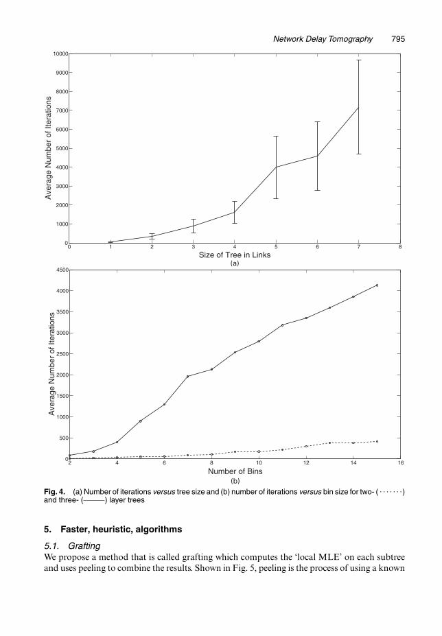
Consider first the effect of the tree size, in terms of both number of links and layers. Westart with a two-layer symmetric binary tree so that there is a total of three links. Then, weadd two children at a time. So the five-link tree corresponds to adding two children to oneof the receiver nodes. The seven-link tree adds two children to the other receiver nodes (sothis is just a three-layer symmetric binary tree). We proceed in this manner until we obtainthe four-layer symmetric binary tree with 15 links (see the x-axis of Fig. 4(a)). The remainingmodel components are held fixed. In particular, each link has a five-bin uniform delay dis-tribution that is chosen because it provides maximum entropy; thus it is the most difficult toresolve. We use a flexicast experiment that is a minimal set of bicast schemes that satisfy theidentifiability conditions. Some additional studies indicated that convergence for the EM algo-rithm does not seem to depend greatly on the number of probes that are used. Hence, in theseinvestigations, each bicast scheme used 1000 probes for each link in its subtree. For each treesize, 50 sets of data were generated and used for estimation. The convergence criterion was achange in the log-likelihood of less than 10−4. Fig. 4(a) shows the number of iterations thatare required for convergence for each data set. The average number of iterations for each sizeis plotted with standard deviation error bars. This suggests that the average number of itera-tions seems to be increasing at a rate that is faster than linear (perhaps exponential) with thenumber of links. This is a further indication that the EM algorithm does not scale well to largernetworks.

Next, consider the effect of the number of bins in each link with uniform delay distributions.The number of bins on each link was varied from 2 to 15. We considered both two-layer andthree-layer binary symmetric trees with three and seven links respectively. Again, a minimalbicast experiment with 1000 probes per scheme was used. The results for both trees are shownin Fig. 4(b). In this scenario, the average number of iterations seems to grow approximatelylinearly with the number of bins on each link. This is an important observation that we shallexploit later in developing a faster algorithm.

4.5. Asymptotic properties of the maximum likelihood estimatorGiven the multinomial nature of the underlying k-cast schemes, the asymptotic properties ofthe maximum likelihood estimator (MLE) mostly follow from general principles. The differencearises because the flexicast experiments imply that individual probes are not independent andidentically distributed. The proposition below establishes that the Fisher information matrixis positive definite at the true value �α0. Thus, the likelihood has a unique maximum in a localneighbourhood of the true value �α0.

Proposition 2. The Fisher information matrix I.�α0/ for the MLE based on end-to-end quan-tized measurements from a flexicast experiment C is finite and positive definite.

The proof can be found in Lawrence (2005). The main idea is to treat the Fisher informationas the covariance of the score function and then to consider various hypothetical data sets toestablish that it must be positive definite.

Proposition 3. Let nCj =n→λCj as n→∞ with 0<λCj <1 for j =1, . . . , M. Then, �αMLE → �α0,almost surely, and

√n.�αMLE − �α0/⇒Z, where Z ∼N{�0, I−1.�α/}.

Proposition 3 follows from proposition 2 by using standard arguments (Lawrence, 2005).


Fig. 4. (a) Number of iterations versus tree size and (b) number of iterations versus bin size for two- ( . . . . . . .)and three- ( ) layer trees

5. Faster, heuristic, algorithms

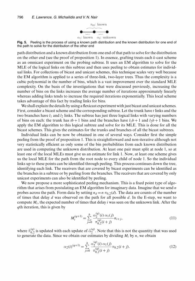
5.1. GraftingWe propose a method that is called grafting which computes the ‘local MLE’ on each subtreeand uses peeling to combine the results. Shown in Fig. 5, peeling is the process of using a known


Fig. 5. Peeling is the process of using a known path distribution and the known distribution for one end ofthe path to solve for the distribution of the other end

path distribution and a known distribution from one end of that path to solve for the distributionon the other end (see the proof of proposition 1). In essence, grafting treats each k-cast schemeas an omnicast experiment on the probing subtree. It uses an EM algorithm to solve for theMLE of the logical links on this subtree and then uses peeling to obtain estimates for individ-ual links. For collections of bicast and unicast schemes, this technique scales very well becausethe EM algorithm is applied to a series of three-link, two-layer trees. Thus the complexity is acubic polynomial in the number of bins, which is a vast improvement over the standard MLEcomplexity. On the basis of the investigations that were discussed previously, increasing thenumber of bins on the links increases the average number of iterations approximately linearlywhereas adding links tends to increase the required iterations exponentially. This local schemetakes advantage of this fact by trading links for bins.

We shall explain the details by using a flexicast experiment with just bicast and unicast schemes.First, consider a bicast scheme and the corresponding subtree. Let the trunk have t links and thetwo branches have l1 and l2 links. The subtree has just three logical links with varying numbersof bins on each: the trunk has tb + 1 bins and the branches have l1b + 1 and l2b + 1 bins. Weapply the EM algorithm to this logical subtree and solve for its MLE. This is done for all thebicast schemes. This gives the estimates for the trunks and branches of all the bicast subtrees.

Individual links can be now be obtained in one of several ways. Consider first the simplepeeling from the proof of proposition 1. This is straightforward and non-iterative although notvery statistically efficient as only some of the bin probabilities from each known distributionare used in computing the unknown distribution. At least one pair must split at node 1, so atleast one of the local MLEs must give us an estimate for link 1. Now, at least one scheme givesus the local MLE for the path from the root node to every child of node 1. So the individuallinks up to these points can be identified through peeling. This process continues down the tree,identifying each link. The receivers that are covered by bicast experiments can be identified asthe branches in a subtree or by peeling from the branches. The receivers that are covered by onlyunicast experiments can also be identified by peeling.

We now propose a more sophisticated peeling mechanism. This is a fixed point type of algo-rithm that arises from postulating an EM algorithm for imaginary data. Imagine that we send n

probes across the path. Form data by setting nd =n π0,2.d/. The data are counts of the numberof times that delay d was observed on the path for all possible d. In the E-step, we want tocompute Mi, the expected number of times that delay i was seen on the unknown link. After theqth iteration, this is given by

M.q+1/i =

b∑j=0

α.q/2 .i/ α1.j/

π.q/0,2.i+ j/

ni+j, .11/

where �π.q/0,2 is updated with each update of �α.q/

2 . Note that this is not the quantity that was usedto generate the data. Since we obtain our estimates by dividing Mi by n, we obtain

α2.i/.q+1/ =b∑

j=0

α.q/2 .i/ α1.j/

π.q/0,2.i+ j/

π0,2.i+ j/: .12/


This equation is no longer based on our imaginary data. It is run until �α2 approaches its fixedpoint. Note that this fixed point algorithm is simply an EM algorithm for computing one linklevel distribution from the path level and other link level distributions and meets standard condi-tions for convergence. Unlike the simple method, this peeling function uses all of the informationfrom the two known distributions.

The peeling method can lead to multiple estimates for some links. The easiest way to addressthis problem is to combine them, using either a simple average or a weighted average. For thelatter, if we have two estimates of �α1 from experiments C1 and C2, we can combine them asfollows to obtain

�̃α1 = nC1 �αC1 +nC2 �αC2

nC1 +nC2: .13/

It can be shown that the grafting algorithm yields estimators that are consistent and asymp-totically normal. The computation of the asymptotic variance is complicated and the simplestway to compute the variance is to use bootstrap or other resampling methods.

5.2. A comparison of the various estimators5.2.1. Other estimators in the literatureTwo other estimation procedures have been proposed in the literature for the delay tomographyproblem. Both are based on omnicast probing and rely on the same modelling assumptions asthose presented here: discrete delay with temporal and spatial independence. The first, whichwas discussed by Lo Presti et al. (2002), depends on solving polynomials. At some link k, theestimator uses the data from the subtree rooted at the link to create a polynomial for each unitof delay, i. The degree of the polynomial is |D.k/|. The second root of this polynomial gives usthe cumulative probability of delay i on link k. The principal drawback of this estimator is thatit does not use all of the information that is available. End-to-end delays that are larger thanthe largest allowable link delay are ignored. Additionally, the nature of the estimator allowsinappropriate results from the polynomial solution such as negative values or values that aregreater than 1.

The estimator by Liang and Yu (2003) is based on a pseudolikelihood approach. The com-plexity of the omnicast experiment is reduced by looking at just bicast projections—all pairwisecombinations—and using a pseudolikelihood that treats them as independent. For example,the network in Fig. 2(b) has 11 receivers, so the omnicast experiment results in 11-dimensionaldelay observations. There are 55 possible pairs of receivers, so the pseudolikelihood schemetreats all the possible pairs of delays as 55 independent bicast observations. The motivatingidea is that processing the data as pairs is computationally much more efficient than processingthe omnicast data. This can be justified if the gain in computational speed offsets the loss instatistical efficiency.

5.2.2. Computational efficiencyComputational speed of the estimators is clearly a major consideration in real applications.Network monitoring requires the ability to solve the inverse estimation problem very quickly.In this section, we investigate the computational efficiencies of the various methods for severaldifferent tree structures. Specifically, we compare the efficiencies of the MLEs based on omnicastprobing, the all-pairs bicast experiment and the ‘minimal plus one’ (min+1) bicast experiment.

Recall that a minimal flexicast experiment refers to a combination of bicast and unicast prob-ing schemes that satisfy the identifiability condition. For a symmetric binary tree, this consists of


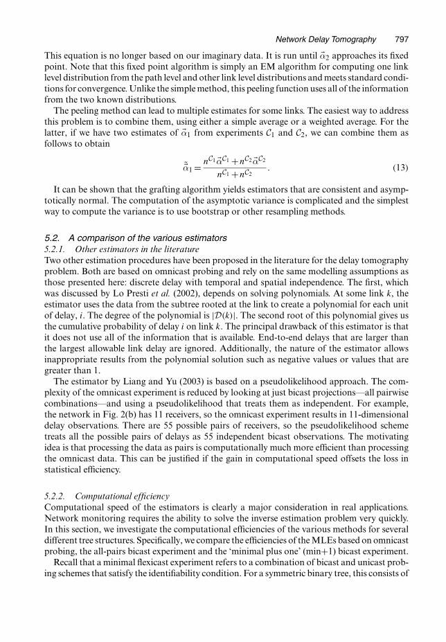
Table 1. Three-layer tree com-parison: average computing time

Estimator Time (s)

MLE 46.93PLE 32.68Polynomial 3.96All-pairs MLE 17.19Min+1 MLE 11.11All-pairs graft 9.11Min+1 graft 5.59

just bicast schemes. To see this, consider the three-layer, binary, symmetric tree in Fig. 2(a). Theminimal bicast experiment is {〈4, 5〉, 〈5, 6〉, 〈6, 7〉}. This experiment is unbalanced as receiverlinks 4 and 7 are covered only once whereas links 5 and 6 are covered twice. A more balancedapproach is obtained by adding pair 〈4, 7〉. This ensures that each link on a particular layerof a binary, symmetric tree is covered by the same number of experiments. We refer to suchexperiments as min+1 flexicast experiments.

In addition to the MLEs, we also consider the pseudolikelihood estimator (PLE), the poly-nomial estimator from Lo Presti et al. (2002) and grafting for all-pairs bicast and min+1 bicastexperiments. All the estimators were implemented by using MATLAB with the combinatorialpartitioning components of the likelihood-based methods written in C. The link delays followa five-bin truncated geometric distribution. The parameters of the distributions were varied ina manner to keep the situations realistic: the interior links have high probability of 0 as com-pared with edge links to simulate the difference between internal links with large bandwidthand smaller local links. The comparisons of efficiency were based on 100 simulated data setsand are shown in Table 1.

The polynomial estimator is, of course, the fastest. This is partially driven by the fact thatit is solving quadratic equations in this example (binary tree) and the formulae for the estim-ates are obtained explicitly. The effect of having a large number of children on the polynomialestimator will be investigated later. We shall also see later that this algorithm can be consid-erably inefficient in a statistical sense. As is to be expected, the PLE is faster than the MLEbased on the full EM algorithm; however, it does not gain as much over the MLE as does thepure bicast algorithm. The all-pairs bicast is more than twice as fast as the likelihood-basedmulticast estimators, whereas the PLE does not seem to benefit from an order of magnitudegain.

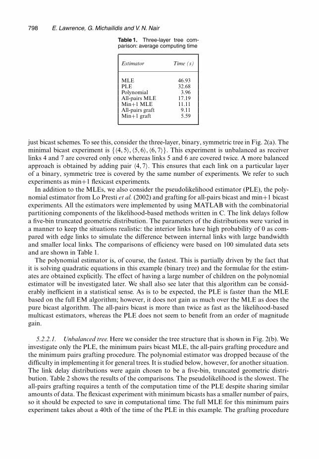
5.2.2.1. Unbalanced tree. Here we consider the tree structure that is shown in Fig. 2(b). Weinvestigate only the PLE, the minimum pairs bicast MLE, the all-pairs grafting procedure andthe minimum pairs grafting procedure. The polynomial estimator was dropped because of thedifficulty in implementing it for general trees. It is studied below, however, for another situation.The link delay distributions were again chosen to be a five-bin, truncated geometric distri-bution. Table 2 shows the results of the comparisons. The pseudolikelihood is the slowest. Theall-pairs grafting requires a tenth of the computation time of the PLE despite sharing similaramounts of data. The flexicast experiment with minimum bicasts has a smaller number of pairs,so it should be expected to save in computational time. The full MLE for this minimum pairsexperiment takes about a 40th of the time of the PLE in this example. The grafting procedure


Table 2. Computational speeds ofestimators applied to data fromFig. 2(b)

Estimator Averagetime (s)

PLE 401.27Minimum 10.12

pairs MLEAll pairs 41.61

graftingMinimum 4.99

pairs grafting

Table 3. Comparison of computa-tion time for grafting and the polyno-mial estimator on shrubs with varyingnumbers of children

Number of Times (s) for thechildren following estimators

Grafting Polynomial

2 0.48 1.026 0.84 1.08

10 0.99 1.13

with minimum pairs is extremely fast, comparable in speed with the time that is achieved by thepolynomial estimator on the simpler tree that was discussed previously.

5.2.2.2. Shrub comparison. Here we investigate only the two fastest estimators: the graftingprocedure with minimum bicast pairs and the polynomial estimator. We study a set of simplecases: shrubs with increasing numbers of children to see how the performance varies. For eachconfiguration, we generated 1000 data sets from truncated geometric distributions on each link.Table 3 lists the average computation times for shrubs with two, six and 10 children. The graftingprocedure is uniformly faster on this test, even when it must combine information from five treesin the 10-child example. The polynomial estimator performs at its best on small trees with smallnumbers of bins. However, when the true bin probability is small, we found that it can lead tonegative estimates in a significant number of cases.

5.2.3. Statistical efficiencyStatistical efficiency has received little attention in the literature, perhaps because of the inher-ent assumption that a large number of probes can be obtained easily. In reality, however, activeexperimentation perturbs the network, and so too much probing in a short period of time canend up causing delay and losses on the network. If we spread the probing over an extendedperiod, it will invalidate the stationarity assumption. As a result, we must limit the number ofprobes, so any effective estimator must be reasonably efficient.


We also note that it is difficult to compare the statistical efficiencies of estimates that are basedon bicast or other flexicast experiments with those that are based on an omnicast experiment asthey are not on an equal footing. If the total number of probes is fixed, the total amount of trafficexpected is different for omnicast and flexicast experiments. Even if we fix the total amount ofexpected traffic on all links under the schemes, different links will have different expected num-bers of probes. It is not possible to make the expected number of probes in each link be thesame under the different schemes. Moreover, omnicast experiments contain information aboutall higher order moments whereas the flexicast experiments are designed to sacrifice the higherorder moments to reduce data complexity.

To keep the comparisons meaningful, we shall examine the efficiencies of estimation meth-ods based on omnicast and bicast experiments separately. The comparisons here are based ona three-layer symmetric binary tree. The link delay distributions were chosen to be truncatedgeometric with five bins.

Fig. 6 shows the performance of the full EM-based MLE, PLE and the polynomial estimatorfor the last bin for three links: α1.4/, α2.4/ and α4.4/. The size of the omnicast experimentwas 20000 total probes. Recall that α1 is the first link on the tree whereas α4 corresponds toone of the receiver nodes. Fig. 6 suggests that the bias is small (medians close to the true values).

Fig. 6. Box plots of the estimates for (a) α1.4/, (b) α2.4/ and (c) α4.4/ for three multicast-based estimators(mean-squared errors are given in parentheses)


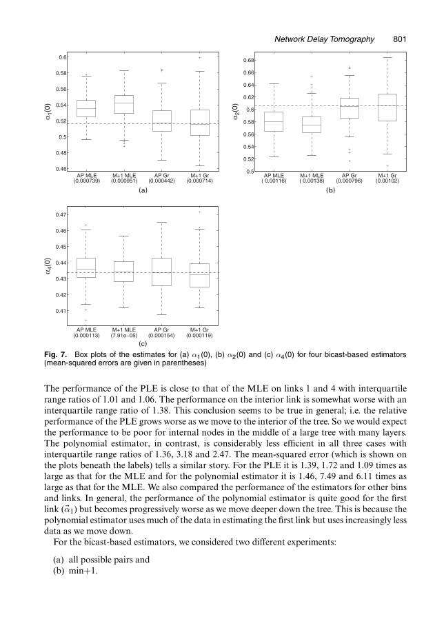
Fig. 7. Box plots of the estimates for (a) α1.0/, (b) α2.0/ and (c) α4.0/ for four bicast-based estimators(mean-squared errors are given in parentheses)

The performance of the PLE is close to that of the MLE on links 1 and 4 with interquartilerange ratios of 1.01 and 1.06. The performance on the interior link is somewhat worse with aninterquartile range ratio of 1.38. This conclusion seems to be true in general; i.e. the relativeperformance of the PLE grows worse as we move to the interior of the tree. So we would expectthe performance to be poor for internal nodes in the middle of a large tree with many layers.The polynomial estimator, in contrast, is considerably less efficient in all three cases withinterquartile range ratios of 1.36, 3.18 and 2.47. The mean-squared error (which is shown onthe plots beneath the labels) tells a similar story. For the PLE it is 1.39, 1.72 and 1.09 times aslarge as that for the MLE and for the polynomial estimator it is 1.46, 7.49 and 6.11 times aslarge as that for the MLE. We also compared the performance of the estimators for other binsand links. In general, the performance of the polynomial estimator is quite good for the firstlink (�α1) but becomes progressively worse as we move deeper down the tree. This is because thepolynomial estimator uses much of the data in estimating the first link but uses increasingly lessdata as we move down.

For the bicast-based estimators, we considered two different experiments:

(a) all possible pairs and(b) min+1.


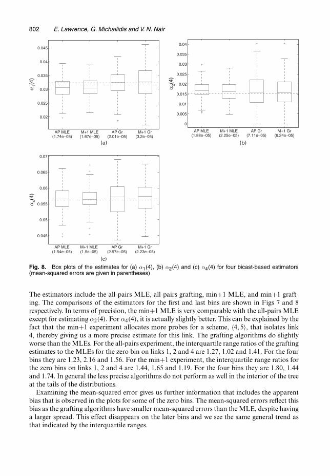
Fig. 8. Box plots of the estimates for (a) α1.4/, (b) α2.4/ and (c) α4.4/ for four bicast-based estimators(mean-squared errors are given in parentheses)

The estimators include the all-pairs MLE, all-pairs grafting, min+1 MLE, and min+1 graft-ing. The comparisons of the estimators for the first and last bins are shown in Figs 7 and 8respectively. In terms of precision, the min+1 MLE is very comparable with the all-pairs MLEexcept for estimating α2.4/. For α4.4/, it is actually slightly better. This can be explained by thefact that the min+1 experiment allocates more probes for a scheme, 〈4, 5〉, that isolates link4, thereby giving us a more precise estimate for this link. The grafting algorithms do slightlyworse than the MLEs. For the all-pairs experiment, the interquartile range ratios of the graftingestimates to the MLEs for the zero bin on links 1, 2 and 4 are 1.27, 1.02 and 1.41. For the fourbins they are 1.23, 2.16 and 1.56. For the min+1 experiment, the interquartile range ratios forthe zero bins on links 1, 2 and 4 are 1.44, 1.65 and 1.19. For the four bins they are 1.80, 1.44and 1.74. In general the less precise algorithms do not perform as well in the interior of the treeat the tails of the distributions.

Examining the mean-squared error gives us further information that includes the apparentbias that is observed in the plots for some of the zero bins. The mean-squared errors reflect thisbias as the grafting algorithms have smaller mean-squared errors than the MLE, despite havinga larger spread. This effect disappears on the later bins and we see the same general trend asthat indicated by the interquartile ranges.


6. Optimal allocation of probes

We now turn to an important issue in designing flexicast experiments, i.e. how to allocate thenumber of probes optimally among the various schemes within a flexicast experiment. The ques-tion of interest is the following: given a fixed budget of probes, how should they be allocatedamong the various flexicast schemes?

It turns out that the optimal allocations depend on the values of the unknown delay distri-butions and the tree topology. This is called local optimality in the design literature (Chernoff,1953). We describe results from a limited study based on binary symmetric trees and bicastschemes to provide some insights and suggest how one could go about studying the problem ingeneral. A comprehensive study of this problem is part of on-going work.

We conduct our study on a three-layer binary symmetric tree (Fig. 2(a)). For each link delaydistribution, we use a geometric distribution truncated to five bins. On the basis of our experiencewith real data and the network simulator, the truncated geometric distribution is a reasonablechoice with its large mass at 0 and decaying tails. We let the parameter of the distributions rangefrom p=0:1 to p=0:9 with a step size of 0:1. This range allows us to consider very good linkswith light tails (p=0:9) and more congested links with heavier tails (p=0:1).

We use the following bicast experiment: C ={〈4, 5〉, 〈6, 7〉, 〈5, 6〉, 〈4, 7〉}. Note that the last twoschemes split at node 1 whereas the first two schemes split at a lower level. We view links 1, 4,5, 6 and 7 as edge links whereas links 2 and 3 will be considered internal or back-bone links.Links of the same type (edge and back-bone) will have the same distribution. On the basis ofthis symmetry, the optimal proportion of probes that are sent to schemes 〈4, 5〉 and 〈6, 7〉 shouldbe equal; likewise for schemes 〈5, 6〉 and 〈4, 7〉. Let τ refer to the total proportion of probes thatare sent to the first group; then the second group will receive a proportion 1 − τ . The designproblem is to identify the optimal value of τ .

The criterion that we use here is D-optimality, which is commonly used in the experimentaldesign literature. Specifically, the optimal value of τ is obtained by maximizing the determin-ant of the Fisher information matrix. As noted before, this value depends on the unknownparameters of the delay distributions, in addition to the tree topology. This is referred to aslocal D-optimality.

First, we consider the optimal τ for the situation in which all the link level distributions areidentical. Interestingly, the optimal value of τ is constant (around 0.75) as p ranges from 0:1 toabout 0:8 and then decreases slightly to about 0:7 as p increases to 0:9. On the basis of this, thebicast pairs 〈4, 5〉 and 〈6, 7〉, which split at a lower level in the tree, should receive about 35–37%of the probes each whereas pairs 〈5, 6〉 and 〈4, 7〉, which split at a higher level, should receiveonly about 12–15% of the probes. Note that the pairs that split at the lower level provide themost information for estimating the receiver links. Further, the total number of probes at eachlink varies: under the above optimal setting, all the probes pass through the link at the top layer,links in layer 2 (the ‘back-bone’ links) each see about three-quarters of the probes, and those atlayer 3 (receiver links) each see only a quarter of the probes.

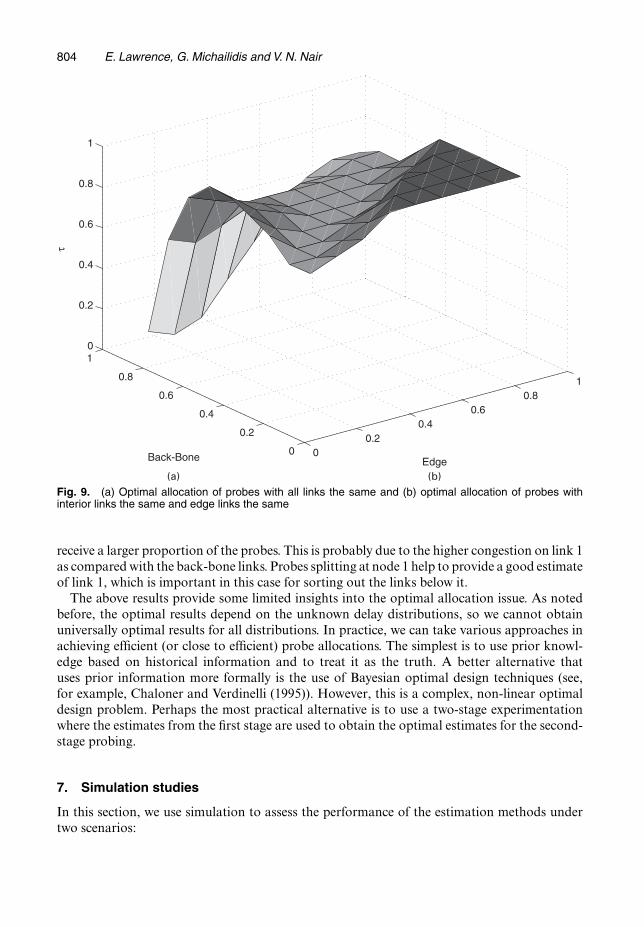
Fig. 9 shows the optimal allocations for a two-dimensional situation: the edge links (link 1and the receiver links) have the same truncated geometric distribution with ‘failure’ probabilityp1 (the x-axis) whereas the back-bone links 2 and 3 have the same distribution with probabilityp2 (the y-axis). The z-axis shows the values of τ , the optimal allocation. For most of the p1 −p2values, the optimal value of τ is between 0.6 and 0.8, again indicating that a higher proportionshould be sent to the bicast pairs that split at the lower level. The exception is, when the failureprobability p2 of the back-bone links becomes larger than about 0.8 and p1 is in the range0.1–0.5, the values of τ decrease, implying that the pairs that split at a higher level should


Fig. 9. (a) Optimal allocation of probes with all links the same and (b) optimal allocation of probes withinterior links the same and edge links the same

receive a larger proportion of the probes. This is probably due to the higher congestion on link 1as compared with the back-bone links. Probes splitting at node 1 help to provide a good estimateof link 1, which is important in this case for sorting out the links below it.

The above results provide some limited insights into the optimal allocation issue. As notedbefore, the optimal results depend on the unknown delay distributions, so we cannot obtainuniversally optimal results for all distributions. In practice, we can take various approaches inachieving efficient (or close to efficient) probe allocations. The simplest is to use prior knowl-edge based on historical information and to treat it as the truth. A better alternative thatuses prior information more formally is the use of Bayesian optimal design techniques (see,for example, Chaloner and Verdinelli (1995)). However, this is a complex, non-linear optimaldesign problem. Perhaps the most practical alternative is to use a two-stage experimentationwhere the estimates from the first stage are used to obtain the optimal estimates for the second-stage probing.

7. Simulation studies

In this section, we use simulation to assess the performance of the estimation methods undertwo scenarios:


(a) under the stochastic model assumptions in Section 2 and(b) using the ns-2 network simulator.

7.1. Model-based simulationOur simulation studies showed that, if the true link level distributions are discrete, the MLE aswell as grafting methods can recover the link level estimates well without any bias. When the truedistributions are continuous, however, the binning seems to introduce some bias. The problemarises from the fact that the end-to-end data are grouped into bins, so we have discretized sumsinstead of sums of discrete values from each link. The extent of the bias depends on the bin size,the link and other variables.

To develop some insights, we considered a three-layer symmetric binary tree (Fig. 2(a)) andfocused on the MLE for a minimum bicast experiment. Each link distribution was taken to bea mixture of exponentials with mean 1 and point mass at 0. The point mass, correspondingto no delay, is common in many real situations. Various bin sizes and point mass probabilitieswere considered in the study. Fig. 10 show the results from links 1, 2 and 4 (link 3 has the same

Fig. 10. Observed (�) and estimated ( ) distributions for links (a) 1, (b) 2 and (c) 4 showing bias whenthe estimation is applied to binned end-to-end data: the distributions are exponential with mean 1 mixed withpoint mass at 0 with probability 0.2; the bin size is 0.25


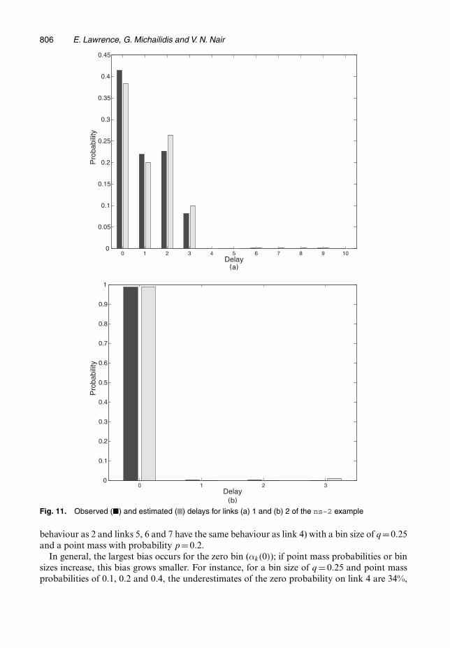
Fig. 11. Observed (�) and estimated ( ) delays for links (a) 1 and (b) 2 of the ns-2 example

behaviour as 2 and links 5, 6 and 7 have the same behaviour as link 4) with a bin size of q=0:25and a point mass with probability p=0:2.

In general, the largest bias occurs for the zero bin (αk.0/); if point mass probabilities or binsizes increase, this bias grows smaller. For instance, for a bin size of q = 0:25 and point massprobabilities of 0.1, 0.2 and 0.4, the underestimates of the zero probability on link 4 are 34%,


24% and 9% respectively. For a bin size of q = 4, the corresponding underestimates reduce to8%, 6% and 4%. Note also from Fig. 10 that the bias is greatest for the receiver node (link 4)and decreases as we go up to the source node.

The effect of this bias on the other bins is much smaller. For the most part, the bias at thezero bin seems to be spread across the rest of the distribution. The estimate at bin 1 seems tocompensate somewhat more than the other bins. There is also some compensation across links;the zero bin for link 1 is overestimated whereas the zero bins for other links are underestimated.We are currently exploring some methods for correcting this bias.

7.2. Network simulationWe now examine the performance of the proposed estimators in a realistic network environmentby using the ns-2 (Information Sciences Institute, 2004) simulation package. This allows usto construct any topology, to generate traffic and to transmit packets by using a real networkprotocol. It gives users control over the hardware and software aspects of a network includingbandwidth, propagation delay, traffic volume and traffic protocol. We constructed the topologythat was shown in Fig. 1 to mimic the UNC network. For links between core routers, we used500 Mbit links and, for links to end points, we used 50 Mbit links. Background traffic on the corelinks consists of 27 transmission control protocol connections and five user datagram protocolconnections. Transmission control protocol connections acknowledge reception of packets bythe receiver. Lost packets are retransmitted by the sender and result in a slower rate of transmis-sion. Therefore, transmission control protocol connections are responsive to congestion. Userdatagram protocol connections do not have any of these features and continue to send packetsat a constant rate, thus being unresponsive to patterns of congestion. On the edge links, thebackground consists of six transmission control protocol connections and one user datagramprotocol connection. The probe traffic consists of 40-bit user datagram protocol packets usingthe multicast protocol.

Every tenth of a second, the probing mechanism selects a scheme at random from C ={〈4, 5〉, 〈6, 7〉, 〈8, 10〉, 〈11, 12〉, 〈13, 14〉, 〈15, 16〉, 〈17, 18〉} and sends a packet to its receivers. Prob-ing lasts for 700 s, resulting in about 1000 packets sent to each pair. This is approximately thelength of a session that we would use for monitoring a real network. The end-to-end delays arediscretized by using a bin size of q = 0:00005s. This is an extremely fine scale, resulting in amaximum link delay setting of b=155. Furthermore, the ns-2 package allows us to record thetrue link delays and hence to obtain directly the link delay distributions for verification.

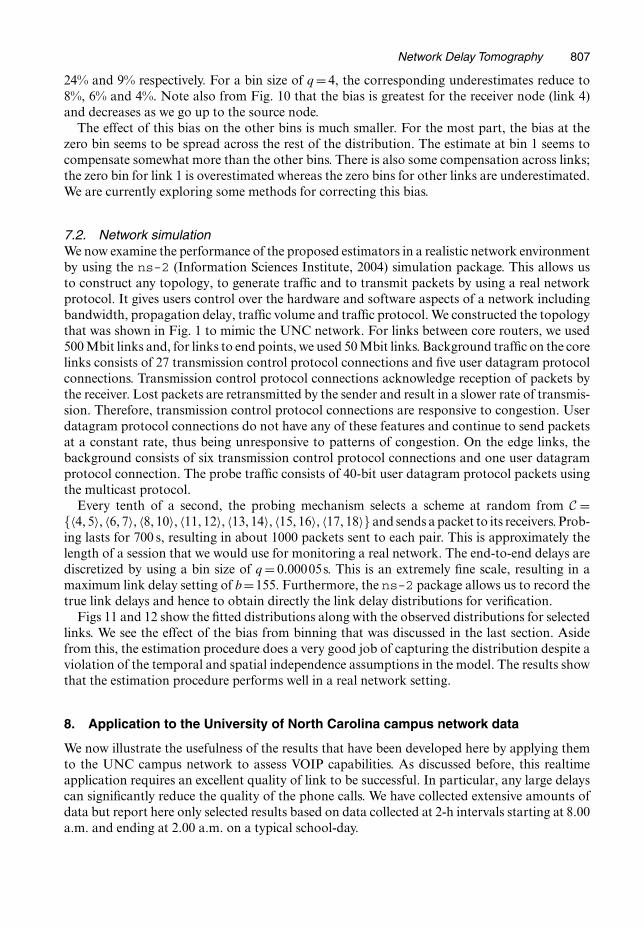
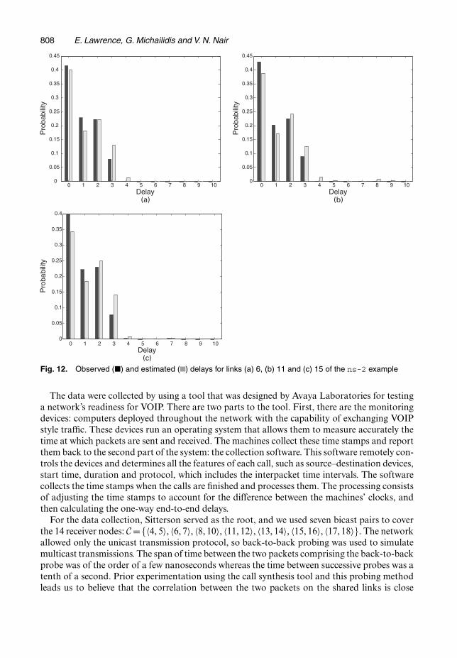
Figs 11 and 12 show the fitted distributions along with the observed distributions for selectedlinks. We see the effect of the bias from binning that was discussed in the last section. Asidefrom this, the estimation procedure does a very good job of capturing the distribution despite aviolation of the temporal and spatial independence assumptions in the model. The results showthat the estimation procedure performs well in a real network setting.

8. Application to the University of North Carolina campus network data

We now illustrate the usefulness of the results that have been developed here by applying themto the UNC campus network to assess VOIP capabilities. As discussed before, this realtimeapplication requires an excellent quality of link to be successful. In particular, any large delayscan significantly reduce the quality of the phone calls. We have collected extensive amounts ofdata but report here only selected results based on data collected at 2-h intervals starting at 8.00a.m. and ending at 2.00 a.m. on a typical school-day.


Fig. 12. Observed (�) and estimated ( ) delays for links (a) 6, (b) 11 and (c) 15 of the ns-2 example

The data were collected by using a tool that was designed by Avaya Laboratories for testinga network’s readiness for VOIP. There are two parts to the tool. First, there are the monitoringdevices: computers deployed throughout the network with the capability of exchanging VOIPstyle traffic. These devices run an operating system that allows them to measure accurately thetime at which packets are sent and received. The machines collect these time stamps and reportthem back to the second part of the system: the collection software. This software remotely con-trols the devices and determines all the features of each call, such as source–destination devices,start time, duration and protocol, which includes the interpacket time intervals. The softwarecollects the time stamps when the calls are finished and processes them. The processing consistsof adjusting the time stamps to account for the difference between the machines’ clocks, andthen calculating the one-way end-to-end delays.

For the data collection, Sitterson served as the root, and we used seven bicast pairs to coverthe 14 receiver nodes: C ={〈4, 5〉, 〈6, 7〉, 〈8, 10〉, 〈11, 12〉, 〈13, 14〉, 〈15, 16〉, 〈17, 18〉}. The networkallowed only the unicast transmission protocol, so back-to-back probing was used to simulatemulticast transmissions. The span of time between the two packets comprising the back-to-backprobe was of the order of a few nanoseconds whereas the time between successive probes was atenth of a second. Prior experimentation using the call synthesis tool and this probing methodleads us to believe that the correlation between the two packets on the shared links is close


Fig. 13. Probability of a large delay on each link throughout the day: (a) Sitterson; (b), (c) core to core;(d) Venable; (e) Davis; (f) McColl; (g) Tarrson; (h) Rosenau; (i) core to core; (j) university library; (k) Everett;(l) Old East; (m) Hinton; (n) Craige; (o) Smith; (p) Greenlaw; (q) South; (r) Phillips

to 1. Each probing session consisted of two passes through the pairs in the order presented.On each pass, each pair was probed for 50 s. Thus, we have 1000 probes for each pair duringeach monitoring session. Maximum likelihood estimation was used to deconvolve the linkdistributions.

In this section, we present results that are related only to discovering links that have signifi-cant probabilities of large delays. For this reason, we used a bin size of q=0:0002 s. Above thisthreshold, delays can become detrimental to the quality of calls. We expect that most links inthis network would have distributions with most of the mass on the zero bin. None-the-less, amass as low as 0.01 on the rest of the delays could prove troublesome.

Fig. 13 shows the probability of delays that are larger than 0.0002 s at various times through-out the day. First, note that the links between the main core routers are of very high quality.The Sitterson outgoing link is also extremely good. The rest of the links do experience somecongestion, varying over the course of the day. Many of the school buildings show a diurnaleffect with large amounts of activity contributing to higher delays starting around noon andcontinuing throughout the afternoon. In particular, there is a little spike around 4.00 p.m. This


Fig. 14. Delay distribution at 12.00 p.m. and 10.00 p.m. for (a) Davis Library, (b) South Building and(c) Hinton Dormitory

spike is evident on link 9 which is a larger core-to-core router. The dormitory links show moreconsistent traffic throughout the entire day with some elevated delays in the later evening. Linksthat show 1% or more large delays would probably require an upgrade to be able to handle theincreased load that is placed on them by VOIP, which uses a more aggressive protocol than theprevalent transmission control protocol traffic. Several receiver links already show close to 5%large delays without a strong VOIP presence. Even the large link 9 seems to be problematic as itneeds to perform almost flawlessly to handle considerably more traffic than the receiver links.

To look at some aspects of the analysis in more detail, we solved the inverse problem using abin size of q=0:00002s for the time periods 12.00 p.m. and 10.00 p.m. This gave us 10 times theresolution of the above analysis. Further, it allowed us to break down the previous analysis tosee where the delays fall within the smallest bin. Fig. 14 shows the first 20 bins of these detailedresults for Davis Library, South Building and Hinton Dormitory. The first thing to note isthat most of the mass is still on the lowest bins so the vast majority of packets experience verylittle delay. Both Davis Library and South Building exhibit a strong diurnal effect. Unlike thedormitory, the traffic in these buildings dies off late at night.

The analyses of other similar data sets that were collected on the network over a period of timeshowed remarkable stability in the results and conclusions. These delay probabilities indicatedto the UNC information technology group that the current network is not capable of support-


ing the VOIP application. From our point of view, the results are qualitatively consistent withthe overall behaviour that is to be expected for this network. This serves as a validation of thetechniques that were studied here, from both statistical and implementation perspectives.

9. Concluding remarks

We have introduced a flexible class of probing experiments for active network tomography andstudied the properties of several methods for estimating the link level delay distributions ofcomputer and communications networks. Both simulation and real data were used to illustratethe usefulness of the methodology. The use of the full EM algorithm is practical for small tomoderate trees, especially with minimum identifiable flexicast experiments (bicast and unicastschemes). With larger networks, the grafting algorithm that was proposed in the paper providesa practical alternative. The fast algorithm is especially useful for monitoring the networks todetect degradation in quality of service and to localize the problem quickly to links or smallregions of the network. We are currently studying monitoring and diagnostic procedures forthis problem.

We have followed the literature in the area in making some simplifying assumptions. Forexample, the logical topology of the network has been assumed to be single source, known andfixed. Extensions to multisource topologies, although conceptually straightforward, neverthe-less introduce technical challenges that are currently under investigation. Further, in practice,the network’s topology can be to a certain degree unknown or changing periodically. Thereis on-going work in the network engineering literature to address these topics. The assump-tion of spatiotemporal stationarity is also commonly made in this area. As we have noted, thetemporal stationarity assumption is not critical as the time between probes is of the order ofmilliseconds. The spatial assumption is more problematic although more realistic models canbe developed only in the context of specific real networks. Additional work is also required toassess the performance of the methods for larger networks. We note, however, that even if theactual network is large, one typically aggregates many of the links and focuses on a smallertopology for studying network performance.

Acknowledgements

The authors thank the Joint Editor, the Associate Editor and two referees for useful commentsand suggestions. The paper is part of the first author’s doctoral dissertation. The research wassupported in part by National Science Foundation grants IIS-9988095, CCR-0325571, DMS-0204247 and DMS-0505535. The authors are grateful to Jim Landwehr, Lorraine Denby andJean Meloche of Avaya Laboratories for making their ExpertNet tool available for VOIP datacollection and for many useful discussions on network monitoring, Yinghan Yang for assis-tance with data collection, Jim Gogan and his team from the Information Technology Divisionat UNC for their technical support in deploying the ExpertNet tool on their campus network,for troubleshooting hardware problems and for providing information about the structure andtopology of the network, Don Smith of the Computer Science Department at UNC for helpingus to establish the collaboration with the UNC information technology group and Steve Marronfor many helpful comments during the course of this research.

Appendix A: Proof of proposition 1

We first establish sufficiency of an omnicast experiment. This will show that an individual k-cast scheme


identifies all the distributions on the paths between source, branching nodes and receivers of its subtrees.We can then show that the above conditions guarantee that we have enough subtrees to solve for everylink delay distribution. The proof of necessity will proceed by contradiction.

For omnicast probing, we consider two cases.

(a) Case 1—receiver node k—consider all omnicast probes that result in zero delay on all remainingreceivers except k. This set of probes allows us to estimate �αk as these probes consist of directobservations from link k.

(b) Case 2—internal node k—we proceed by induction. Suppose that we have identified the distributionsfor all links that are descendants of k. Let R.k/ represent the receivers that are descended from k.Consider probes that result in zero delay on all nodes except those in R.k/ which all experience idelay. Let γk.i/ be the probability that each r ∈R.k/ has an end-to-end delay of i. From this, we canestimate γk.i/ for each i. Since we have estimates of link delay distributions of the descendants of k,we can now estimate �αk.

This proof implies that a single k-cast scheme will identify the following distributions: the path betweenthe source and the first splitting node, the paths between any two splitting nodes and the paths betweena splitting node and a receiver. Now we focus on a collection of flexicast schemes. Here we consider threecases.

(a) Case 1: there is some k-cast scheme Cj in which branching occurs at node 1, the only child of the rootnode. Based on the omnicast identifiability proof, this experiment identifies the delay distributionfor link 1, �α1.

(b) Case 2: let s be some internal node. Assume that we have identified all the delay distributions forlinks k ∈P0,f.s/. There is a scheme Cj for which branching occurs at node s. This scheme identifiesthe path level distribution �π0,s. We can construct �π0,f.s/ and solve for �αs:

αs.0/=π0,s.0/=π0,f.s/,

αs.d/= 1π0,f.s/.0/

{π0,s.d/−

d−1∑δ=max.0, d−Bf.s//

αs.δ/ π0,f.s/.d − δ/

}, ∀d =1, . . . , b,

where Bf.s/ is the maximum delay up to this node. We call this solution peeling since we are peelingthe unknown distribution from the path level distributions. It can be used more generally and cantake other functional forms.

(c) Case 3: let r be some receiver node. Assume that we have identified all the delay distributions forlinks k ∈P0,f.r/. There is some scheme Cj which probes receiver r. From this, we can estimate thepath probability π0, r. We can construct �π0,f.r/ and use peeling to obtain �αr.

It is easy to see the necessity of covering all the receivers: if we do not probe a receiver, we can neverestimate its link delay distribution. To see the necessity of branching at each internal node, consider a col-lection of schemes in which branching occurs at all internal nodes except some node s. Each link d ∈D.s/will always occur as part of a logical link that also includes link s. We will be able to obtain estimates for�πf.s/,d for each d ∈D.s/ but we shall have no information with which to peel the two apart. In essence,these estimates are like unicast measurements which are not sufficient for estimation.

References

Cáceres, R., Duffield, N. G., Horowitz, J. and Towsley, D. F. (1999) Multicast-based inference of network-internalloss characteristics. IEEE Trans. Inform. Theory, 45, 2462–2480.

Cao, J., Davis, D., Vander Wiel, S. and Yu, B. (2000) Time-varying network tomography: router link data. J. Am.Statist. Ass., 95, 1063–1075.

Castro, R., Coates, M., Liang, G., Nowak, R. and Yu, B. (2004) Network tomography: recent developments.Statist. Sci., 19, 499–517.

Chaloner, K. and Verdinelli, I. (1995) Bayesian experimental design: a review. Statist. Sci., 10, 273–304.Chernoff, H. (1953) Locally optimal designs for estimating parameters. Ann. Math. Statist., 24, 586–602.Information Sciences Institute (2004) The Network Simulator. Marina del Rey: Information Sciences Institute.

(Available from http://www.isi.edu/nsnam/ns/.)Lawrence, E. (2005) Flexicast network delay tomography. PhD Thesis. University of Michigan, Ann Arbor.Liang, G. and Yu, B. (2003) Maximum pseudo likelihood estimation in network tomography. IEEE Trans. Signal

Process., 51, 2043–2053.


Lo Presti, F., Duffield, N. G., Horowitz, J. and Towsley, D. (2002) Multicast-based inference of network-internaldelay distributions. IEEE Trans. Netwrkng, 10, 761–775.

Shih, M.-F. and Hero, A. O. (2003) Unicast-based inference of network link delay distributions with finite mixturemodels. IEEE Trans. Signal Process., 51, 2219–2228.

Tebaldi, C. and West, M. (1998) Bayesian inference on network traffic using link count data. J. Am. Statist. Ass.,93, 557–573.

Vardi, Y. (1996) Network tomography: estimating source-destination traffic intensities from link data. J. Am.Statist. Ass., 91, 365–377.

Xi, B., Michailidis, G. and Nair, V. N. (2007) Estimating network loss rates using active tomography. J. Am.Statist. Ass., to be published.

Zhang, Y., Roughan, M., Lund, C. and Donoho, D. (2003) An information-theoretic approach to traffic matrixestimation. In Proc. A. Conf. Special Interest Group on Data Communication, Karlsruhe. New York: Associationfor Computing Machinery Press.

Network delay tomography using ï¬‚exicast experiments

Documents

Transcript of Network delay tomography using ï¬‚exicast experiments