Graduate Theses and Dissertations Iowa State University Capstones, Theses andDissertations

2018

Network coding for function computationArdhendu Shekhar TripathyIowa State University

Follow this and additional works at: https://lib.dr.iastate.edu/etd

Part of the Electrical and Electronics Commons, Library and Information Science Commons,and the Mathematics Commons

This Dissertation is brought to you for free and open access by the Iowa State University Capstones, Theses and Dissertations at Iowa State UniversityDigital Repository. It has been accepted for inclusion in Graduate Theses and Dissertations by an authorized administrator of Iowa State UniversityDigital Repository. For more information, please contact digirep@iastate.edu.

Recommended CitationTripathy, Ardhendu Shekhar, "Network coding for function computation" (2018). Graduate Theses and Dissertations. 16476.https://lib.dr.iastate.edu/etd/16476

Network coding for function computation

by

Ardhendu Shekhar Tripathy

A dissertation submitted to the graduate faculty

in partial fulfillment of the requirements for the degree of

DOCTOR OF PHILOSOPHY

Major: Electrical and Computer Engineering

Program of Study Committee:Aditya Ramamoorthy, Major Professor

Nicola EliaChinmay HegdeSung-Yell SongZhengdao Wang

The student author, whose presentation of the scholarship herein was approved by the program ofstudy committee, is solely responsible for the content of this dissertation. The Graduate Collegewill ensure this dissertation is globally accessible and will not permit alterations after a degree is

conferred.

Iowa State University

Ames, Iowa

2018

Copyright c© Ardhendu Shekhar Tripathy, 2018. All rights reserved.

ii

TABLE OF CONTENTS

Page

LIST OF TABLES . . . . . . . . . . . . . . . . . . . . . . . . . . . . . . . . . . . . . . . . . . iv

LIST OF FIGURES . . . . . . . . . . . . . . . . . . . . . . . . . . . . . . . . . . . . . . . . . vi

ACKNOWLEDGEMENTS . . . . . . . . . . . . . . . . . . . . . . . . . . . . . . . . . . . . . viii

ABSTRACT . . . . . . . . . . . . . . . . . . . . . . . . . . . . . . . . . . . . . . . . . . . . . x

CHAPTER 1. INTRODUCTION . . . . . . . . . . . . . . . . . . . . . . . . . . . . . . . . . 1

1.1 Function computation: Sum-networks . . . . . . . . . . . . . . . . . . . . . . . . . . 1

1.2 Function computation: Using variable-length network codes . . . . . . . . . . . . . . 3

CHAPTER 2. SUM-NETWORKS FROM INCIDENCE STRUCTURES . . . . . . . . . . . 4

2.1 Introduction . . . . . . . . . . . . . . . . . . . . . . . . . . . . . . . . . . . . . . . . . 4

2.2 Background, related work and summary of contributions . . . . . . . . . . . . . . . . 8

2.2.1 Summary of contributions . . . . . . . . . . . . . . . . . . . . . . . . . . . . . 9

2.3 Problem formulation and preliminaries . . . . . . . . . . . . . . . . . . . . . . . . . . 10

2.4 Construction of a family of sum-networks . . . . . . . . . . . . . . . . . . . . . . . . 15

2.5 Upper bound on the computation capacity . . . . . . . . . . . . . . . . . . . . . . . . 19

2.6 Linear network codes for constructed sum-networks . . . . . . . . . . . . . . . . . . . 32

2.7 Discussion and comparison with prior work . . . . . . . . . . . . . . . . . . . . . . . 48

2.7.1 Comparison with prior work . . . . . . . . . . . . . . . . . . . . . . . . . . . . 52

2.8 Conclusions and future work . . . . . . . . . . . . . . . . . . . . . . . . . . . . . . . 53

iii

CHAPTER 3. FUNCTION COMPUTATION ON A DIRECTED ACYCLIC NETWORK . 54

3.1 Introduction . . . . . . . . . . . . . . . . . . . . . . . . . . . . . . . . . . . . . . . . . 54

3.1.1 Related work . . . . . . . . . . . . . . . . . . . . . . . . . . . . . . . . . . . . 58

3.1.2 Main contributions . . . . . . . . . . . . . . . . . . . . . . . . . . . . . . . . . 60

3.2 Problem formulation . . . . . . . . . . . . . . . . . . . . . . . . . . . . . . . . . . . . 60

3.2.1 Variable-length network code for network in figure 3.1 . . . . . . . . . . . . . 65

3.3 Bounds on the rate region for network in figure 3.1 . . . . . . . . . . . . . . . . . . . 66

3.3.1 Lower bound on the conditional entropy . . . . . . . . . . . . . . . . . . . . . 69

3.3.2 Value of α . . . . . . . . . . . . . . . . . . . . . . . . . . . . . . . . . . . . . . 83

3.3.3 Example demand function: Arithmetic sum . . . . . . . . . . . . . . . . . . . 84

3.3.4 Example demand function: Sum over GF (2) . . . . . . . . . . . . . . . . . . 92

3.4 Conclusions and future work . . . . . . . . . . . . . . . . . . . . . . . . . . . . . . . 93

CHAPTER 4. CONCLUSIONS AND FUTURE WORK . . . . . . . . . . . . . . . . . . . . 95

4.1 Future work . . . . . . . . . . . . . . . . . . . . . . . . . . . . . . . . . . . . . . . . . 97

BIBLIOGRAPHY . . . . . . . . . . . . . . . . . . . . . . . . . . . . . . . . . . . . . . . . . . 98

APPENDIX A. NON-APPLICABILITY OF THEOREM VI.5 IN [8] FOR SUM-NETWORKS102

APPENDIX B. PROOF OF LEMMA 6 IN CHAPTER 3 . . . . . . . . . . . . . . . . . . . . 106

APPENDIX C. CALCULATION FOR EQUATION (3.12) . . . . . . . . . . . . . . . . . . . 107

APPENDIX D. LIST OF PUBLICATIONS FROM DISSERTATION . . . . . . . . . . . . . 109

iv

LIST OF TABLES

Page

2.1 The function values transmitted across e1, e2 in Figure 2.2a for a network

code with rate = 2/3. Each message X1, X2, X{1,2} is a vector with 2 com-

ponents, and φ1(X), φ2(X) are vectors with 3 components each. A number

within square brackets adjoining a vector indicates a particular component

of the vector. . . . . . . . . . . . . . . . . . . . . . . . . . . . . . . . . . . . 33

2.2 The function values transmitted across e1, e2, e3, e4 in Figure 2.5b for a net-

work code with rate = 4/9. Each message XA, XB, XC , XD, XE is a vec-

tor with 4 components, and φ1(X), φ2(X), φ3(X), φ4(X) are vectors with

9 components each. The number inside square brackets adjoining a vector

indicates a particular component of the vector. . . . . . . . . . . . . . . . . 40

2.3 The function values transmitted across the bottleneck edges of the trans-

posed sum-network corresponding to the graph shown in Figure 2.5a for

a rate-4/6 network over GF (2). Each message X2, X4 is a vector with 4

components, and φA(X), φB(X), φC(X), φD(X), φE(X) are vectors with 6

components each. The number inside square brackets adjoining a vector

indicates a particular component of the vector. A dash indicates that the

value transmitted on that component is not used in decoding by any terminal. 44

3.1 Function table for a demand function to be computed over the network in

Figure 3.1. The message alphabet is A = GF (3). Table 3.1a shows the

function values for all (X1, X2) pairs when X3 = 0, table 3.1b shows the

function values when X3 = 1 and table 3.1c shows the function values when

X3 = 2. . . . . . . . . . . . . . . . . . . . . . . . . . . . . . . . . . . . . . . 71

v

3.2 The sets V12(a3, b) for different values of the demand function realization b

and different values of a3 in different rows. . . . . . . . . . . . . . . . . . . . 78

vi

LIST OF FIGURES

Page

1.1 Communication networks represented as directed acyclic graphs. . . . . . . . 2

2.1 A pictorial depiction of the Fano plane. The point set P = {1, . . . , 7}. The

blocks are indicated by a straight line joining their constituent points. The

points 2, 4 and 6 lying on the circle also depict a block. . . . . . . . . . . . . 14

2.2 Two sum-networks obtained from the line graph on two vertices described

in Example 2. The source set S and the terminal set T contain three nodes

each. All edges are unit-capacity and point downward. The edges with the

arrowheads are the bottleneck edges constructed in step 2 of the construction

procedure. (a) Normal sum-network, and (b) transposed sum-network. . . . 18

2.3 The normal sum-network obtained for the incidence structure I described

in Example 3. All edges are unit-capacity and directed downward. The

edges with the arrowheads are the bottleneck edges, and the edges denoted

by dashed lines correspond to the direct edges introduced in step 4 of the

construction procedure. For this case, the normal and the transposed sum-

network are identical. . . . . . . . . . . . . . . . . . . . . . . . . . . . . . . . 19

2.4 A simple undirected graph G with two connected components. It has 6

vertices and 4 edges. . . . . . . . . . . . . . . . . . . . . . . . . . . . . . . . 27

vii

2.5 (a) Undirected graph considered in Example 7. (b) Part of the correspond-

ing normal sum-network constructed for the undirected graph in (a). The

full normal sum-network has nine nodes each in the source set S and the

terminal set T . However, for clarity, only the five sources and terminals that

correspond to the columns of the incidence matrix of the graph are shown.

Also, the direct edges constructed in Step 4 of the construction procedure

are not shown. All edges are unit-capacity and point downward. The edges

with the arrowheads are the bottleneck edges constructed in step 2 of the

construction procedure. (c) Bipartite flow network as constructed in the

proof of theorem 4 for this sum-network. The message values corresponding

to the flow on the solid lines are also shown. . . . . . . . . . . . . . . . . . 39

2.6 The schematic shown represents an undirected graph with three components:

S6, S14 and S10. St denotes the star graph on t+ 1 vertices, with only one

vertex having degree t while the rest have degree 1. The vertices with the

maximum degree in the three star graphs are a, b, c respectively. In addition,

a is connected to b and b is connected to c, such that deg(a) = 7,deg(b) =

16, deg(c) = 11. . . . . . . . . . . . . . . . . . . . . . . . . . . . . . . . . . . 50

3.1 A directed acyclic network with three sources, two of which also act as relay

nodes, and one terminal. . . . . . . . . . . . . . . . . . . . . . . . . . . . . 61

3.2 A directed acyclic network with two sources, four relay nodes and one ter-

minal. . . . . . . . . . . . . . . . . . . . . . . . . . . . . . . . . . . . . . . . 64

A.1 A simple sum-network. Both edges can transmit one symbol in F1 from tail

to head in one channel use. . . . . . . . . . . . . . . . . . . . . . . . . . . . . 103

viii

ACKNOWLEDGEMENTS

I would like to thank my advisor Prof. Aditya Ramamoorthy for his steadfast help and men-

torship throughout my Ph.D. degree. I have learned a lot from him. How to formulate a good

problem, ways to identify and obtain the parts necessary for a particular approach to the problem,

and how to salvage something useful from failed attempts or unruly intuition — all of these have

surfaced more than a few times during my research and I have been aided greatly by my advisor’s

guidance in these. His technical knowledge has steered me in the choice of subjects I have studied

here, many ideas from which have found application in this dissertation. He has also helped me

improve my writing and presentation skills. That has helped me effectively communicate my work

in seminars at Iowa State, as well as national and international meetings.

I have also greatly enjoyed the interactions I have had with my committee members. Prof.

Zhengdao Wang has always been enthusiastic about my research and has given me great feedback.

Some of the directions explored here were prompted by his questions. I have enjoyed attending

many of the courses he has taught here. Prof. Chinmay Hegde has been a friend and a mentor to

me. I have always felt welcome to discuss my research and various other topics in his office. He

has been very interested in my research and has always encouraged me. Prof. Nicola Elia has been

a careful listener and has asked questions that have improved my understanding of the problems

I have worked on. Prof. Sung-Yell Song has taught me much of the new mathematics that I have

learned at Iowa State University. He has been interested and inquisitive about the way it has found

applications in engineering.

Some other faculty with whom I have often talked about academic matters separate from my

dissertation research are Prof. Namrata Vaswani and Prof. Yongxin Chen. They have always

provided me good advice. Prof. Pavan Aduri, Prof. Jin Tian and Prof. Leslie Hogben have been

patient in answering the many questions that I have asked them.

ix

The work in this dissertation was funded in part by the National Science Foundation (NSF)

under the following grants — CCF-1149860, CCF-1320416 and CCF-1718470. The support of the

NSF is gratefully acknowledged.

Through the years in Coover Hall, I have enjoyed the company and discussions I have had with

Hooshang Ghasemi, Li Tang and Konstantinos Konstantinidis. I am also glad to have known a

wider group of graduate students who have been eager to listen and converse. Han Guo, Seyedehsara

Nayer, Praneeth Narayanamurthy, Zhengyu Chen, Vahid Daneshpajooh, Mohammadreza Soltani,

Gauri Jagatap, Thanh Nguyen, Viraj Shah, Songtao Lu, Pan Zhong, Qi Xiao, Rahul Singh, and

the many others who have been involved in the Data Science Reading Group — I have greatly

enjoyed it and I hope it continues. Apurba Das was willing to discuss research patiently, in spite

of our very different research areas. I also thank Mohammadreza, Praneeth and Songtao for their

help and support in matters outside of academics. The student workers and staff in the ECpE main

office and student services office have been helpful and pleasant in all my requests to them. I owe

a debt to Cover and Thomas, the 1991 edition of their textbook inspired me to do research in this

area.

Outside of Coover Hall, there have been a group of close friends who have helped me weather the

tides of graduate student life. They are Srijita Patra, Siva Konduri, Priyanka Bolel, Rhitajit Sarkar,

Neelam Prabhu-Gaunkar, Viksit Kumar, Sophiya Das, Jayaprakash Selvaraj, Priyam Rastogi, Sai

Pushpak, Sangeetha N.S., and Aneesh Rajendran. I have good memories from the times we spent

together.

This dissertation would not have been possible without the love and affection of my girlfriend

Niranjana Krishnan and my family in India. My parents and sister have always believed in my

abilities and supported me. I owe to them and Niranjana my biggest thanks.

x

ABSTRACT

Many applications such as parallel processing, distributed data analytics and sensor networks

often need to compute functions of data that are observed in a distributed manner over a network.

A network can be modeled as a directed graph, each vertex of which denotes a node that can carry

out computations and communicate with its neighbors. The edges of the graph denote one-way

noiseless communication links. A subset of nodes - called sources - observe independent messages,

and a possibly different subset of nodes - called terminals - wish to compute a particular demand

function of the messages. The information transmitted on the edges are specified by a set of

functions, one for each edge; this set of functions is called a network code. We are interested in

network codes that allow each terminal to compute the demanded function with zero-error.

In the first part of this thesis, we assume that the message random variables are independent

and uniformly distributed over a finite field. The demand function is set to be the finite field sum of

all the messages observed in the network. A valid network code for this sum-network problem allows

each terminal to compute the sum, and has an associated computation rate. We wish to find the

best possible computation rate for a given sum-network; this value is called its computation capacity.

Finding the computation capacity of a sum-network is known to be a difficult problem. Here we

are able to evaluate it for certain systematically constructed sum-network problem instances. The

construction procedure uses incidence structures, whose combinatorial properties allow us to be

able to evaluate the computation capacity of the constructed sum-networks. An important aspect

of the problem that we uncover is the strong dependence of the computation capacity on the finite

field over which the sum is to computed. This is shown by a sum-network, whose computation

capacity is 1 over a finite field and close to 0 over a different finite field. We also construct sum-

networks whose computation capacity can take on arbitrarily many different values over different

finite field alphabets.

xi

In the second part of the thesis, we focus on a particular directed acyclic network that has four

nodes and four edges. It is the simplest instance of a network that does not have a tree structure.

Three of the nodes are sources that observe independent messages that are uniformly distributed

over a finite discrete alphabet. The fourth node is a terminal which wants to compute a demand

function of the three messages. The demand function is an arbitrary discrete-valued function. We

focus on network codes that have different rates on each of the four edges, thus we have a rate tuple

associated with every valid network code. The collection of rate tuples for all valid network codes

form a rate region, and we describe a procedure to obtain an outer bound to this rate region. We

illustrate our approach through different example demand functions. When the demand function is

the finite field sum over GF (2), we give a network code whose rate tuple matches the outer bound.

1

CHAPTER 1. INTRODUCTION

The unprecedented scale of data generation, storage and analysis in present times is a well-

known phenomenon. Coupled with the formation of networks of such data nodes, this situation has

posed ample engineering challenges and opened new possibilities. Complementary to speeding up

data processing and connectivity speeds, one could consider the following question: how efficiently

can we combine data over a network?

Consider a network of temperature sensors in a centrally air-conditioned building. The control

unit would take in the temperature readings, i.e., the data, and perform some computation on them

to decide whether to heat or cool the building. Thus, interpreting and making useful conclusions of

the data can be thought of as computing certain functions on the data. Finding optimal procedures

and fundamental limits on how efficiently this can be done is important for increasingly large

datasets.

1.1 Function computation: Sum-networks

Sum-networks are a class of function computation problems over networks. We represent a

communication network by a directed acyclic graph, as shown in Figure 1.1a. The structure of the

graph is a part of the problem description.

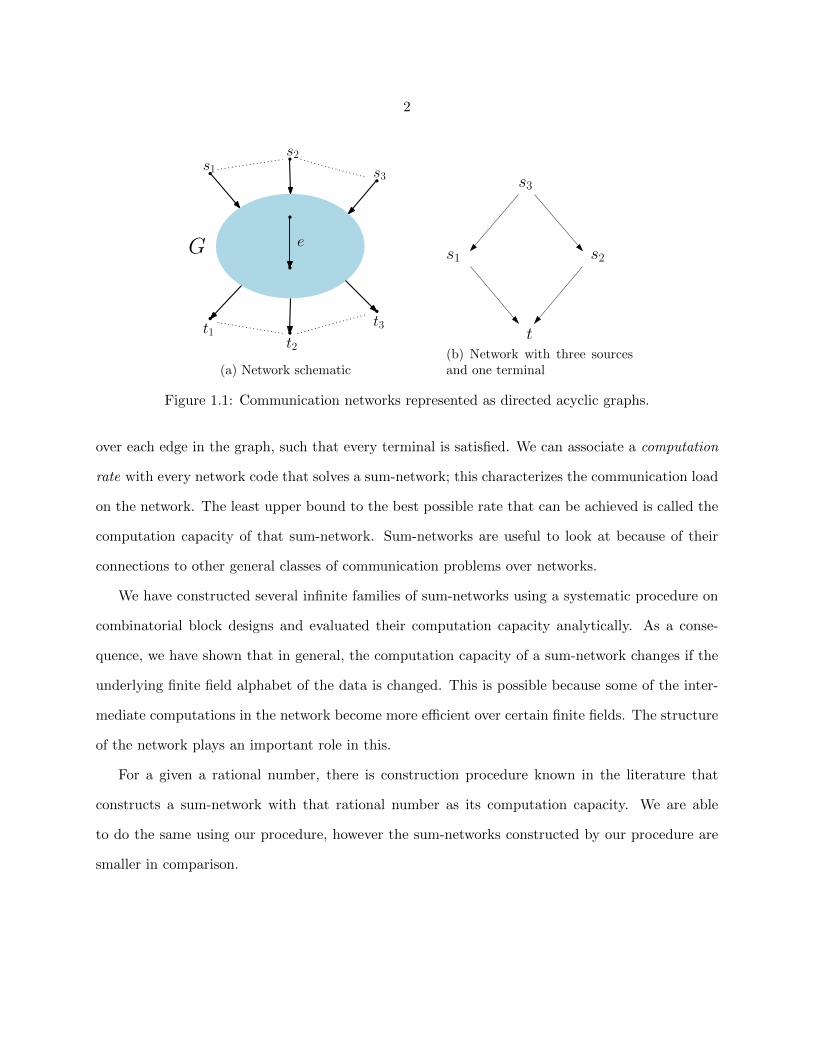
The two components of the graph, i.e., its vertices and edges denote nodes in a network and the

communication links between them, respectively. A subset of the nodes called the sources, denoted

as s1, s2 and s3, observe independent data, which are assumed to be elements of a finite field. A

different subset of nodes called the terminals, are denoted as t1, t2, t3 and each of them wants to

compute with zero error the finite field sum of all the data observed at the source nodes. The edges

in the network, shown as e, are one-way communication links that are error-free. The objective is to

come up with a scheme, called a network code, that specifies what descriptions are to be transmitted

2

G

s1s2

s3

t1t2

t3

e

(a) Network schematic

s3

s1 s2

t(b) Network with three sourcesand one terminal

Figure 1.1: Communication networks represented as directed acyclic graphs.

over each edge in the graph, such that every terminal is satisfied. We can associate a computation

rate with every network code that solves a sum-network; this characterizes the communication load

on the network. The least upper bound to the best possible rate that can be achieved is called the

computation capacity of that sum-network. Sum-networks are useful to look at because of their

connections to other general classes of communication problems over networks.

We have constructed several infinite families of sum-networks using a systematic procedure on

combinatorial block designs and evaluated their computation capacity analytically. As a conse-

quence, we have shown that in general, the computation capacity of a sum-network changes if the

underlying finite field alphabet of the data is changed. This is possible because some of the inter-

mediate computations in the network become more efficient over certain finite fields. The structure

of the network plays an important role in this.

For a given a rational number, there is construction procedure known in the literature that

constructs a sum-network with that rational number as its computation capacity. We are able

to do the same using our procedure, however the sum-networks constructed by our procedure are

smaller in comparison.

3

1.2 Function computation: Using variable-length network codes

Consider now a more specific network shown in Figure 1.1b. Suppose each source observes a

data value that is either 0 or 1, and the terminal wishes to compute with zero error the sum, over

the real numbers, of the three data values. This is the simplest non-tree network structure, and its

computation capacity is known to be log6 4 ≈ 0.77 in the standard network code framework. This

value is obtained after counting the necessary and sufficient number of distinct messages that are

transmitted over the edges (s1, t) and (s2, t).

Suppose now that each of the data values is known to be equally likely to be 0 or 1. A traditional

network code assigns the same amount of communication resources for each edge and each block

of data values. However, by relaxing this requirement, i.e., by letting the edge messages have

variable-length based on the current block of data values, we can use the probability information

to compress the number of bits that can be represented in the messages. This allows us to reduce

the communication load; in this example, we demonstrate a network code with rate 0.8 in the

variable-length network code framework. We describe a method to obtain an upper bound to the

rate in the variable-length code framework. This method is general and can be applied to arbitrary

demand functions.

Previous literature on computation capacity in the variable-length framework is only applicable

to either tree-networks or networks in which the sources are directly connected to the terminal. For

directed acyclic graph networks, existing literature has mainly focused on finding the computation

capacity in the standard fixed-length network code framework.

4

CHAPTER 2. SUM-NETWORKS FROM INCIDENCE STRUCTURES

1 A sum-network is an instance of a function computation problem over a directed acyclic

network in which each terminal node wants to compute the sum over a finite field of the information

observed at all the source nodes. Many characteristics of the well-studied multiple unicast network

communication problem also hold for sum-networks due to a known reduction between the two

problems. In this work, we describe an algorithm to construct families of sum-network instances

using incidence structures. The computation capacity of several of these sum-network families is

evaluated. Unlike the coding capacity of a multiple unicast problem, the computation capacity of

sum-networks depends on the characteristic of the finite field over which the sum is computed. This

dependence is very strong; we show examples of sum-networks that have a rate-1 solution over one

characteristic but a rate close to zero over a different characteristic. Additionally, a sum-network

can have arbitrarily different computation capacities for different alphabets.

2.1 Introduction

Applications as diverse as parallel processing, distributed data analytics and sensor networks

often deal with variants of the problem of distributed computation. This has motivated the study

of various problems in the fields of computer science, automatic control and information theory.

Broadly speaking, one can model this question in the following manner. Consider a directed

acyclic network with its edges denoting communication links. A subset of the nodes observe certain

information, these nodes are called sources. A different subset of nodes, called terminals, wish to

compute functions of the observed information with a certain fidelity. The computation is carried

out by the terminals with the aid of the information received over their incoming edges. The demand

1This chapter is adapted from an article published in the IEEE Transactions on Information Theory. Parts of thiswork have been presented at the 52nd Allerton Conference on Communication, Control and Computing, 2014 andthe 2015 IEEE International Symposium on Information Theory.

5

functions and the network topology are a part of the problem instance and can be arbitrary. This

framework is very general and encompasses several problems that have received significant research

attention.

Prior work [1],[2],[3] concerning information theoretic issues in function computation worked

under the setting of correlated information observed at the sources and simple network structures,

which were simple in the sense that there were edges connecting the sources to the terminal without

any intermediate nodes or relays. For instance, [2] characterizes the amount of information that a

source must transmit so that a terminal with some correlated side-information can reliably compute

a function of the message observed at the source and the side-information. Reference [3] considered

distributed functional compression, in which two messages are separately encoded and given to a

decoder that computes a function of the two messages with an arbitrarily small probability of error.

With the advent of network coding [4],[5], the scope of the questions considered included the

setting in which the information observed at the sources is independent and the network topology

is more complex. Under this setting, information is sent from a source to a terminal over a path of

edges in the directed acyclic network with one or more intermediate nodes in it, these relay nodes

have no limit on their memory or computational power. The communication edges are abstracted

into error-free, delay-free links with a certain capacity for information transfer and are sometimes

referred to as bit-pipes. The messages are required to be recovered with zero distortion. The

multicast scenario, in which the message observed at the only source in the network is demanded

by all terminals in the network, is solved in [4],[5],[6]. A sufficient condition for solvability in

the multicast scenario is that each terminal has a max-flow from the source that is at least the

entropy rate of the message random process [4]. Reference [6] established that linear network codes

over a sufficiently large alphabet can solve this problem and [5] provided necessary and sufficient

conditions for solving a multicast problem instance in an algebraic framework. The work in [5] also

gave a simple algorithm to construct a network code that satisfies it.

Unlike the multicast problem, the multiple unicast problem does not admit such a clean solution.

This scenario has multiple source-terminal pairs over a directed acyclic network of bit-pipes and

6

each terminal wants to recover the message sent by its corresponding source with the help of the

information transmitted on the network. To begin with, there are problem instances where more

than one use of the network is required to solve it. To model this, each network edge is viewed as

carrying a vector of n alphabet symbols, while each message is a vector of m alphabet symbols. A

network code specifies the relationship between the vector transmitted on each edge of the network

and the message vectors, and it solves a network coding problem instance if m = n. It is shown

that linear network codes are in general not sufficient to solve this problem [7]. One can define the

notion of coding capacity of a network as the supremum of the ratio m/n over all network codes

that allow each terminal to recover its desired message; this ratio m/n for a particular network

code is called its rate. The coding capacity of a network is independent of the alphabet used [8].

While a network code with any rational rate less than the coding capacity exists by definition

and zero-padding, a network code with rate equal to coding capacity does not exist for certain

networks, even if the coding capacity is rational [9]. The multi-commodity flow solution to the

multiple unicast problem is called a routing solution, as the different messages can be interpreted

as distinct commodities routed through the intermediate nodes. It is well-known that in the case

of multicast, network coding can provide a gain in rate over traditional routing of messages that

scales with the size of the network [10]. However, evaluating the coding capacity for an arbitrary

instance of the network coding problem is known to be hard in general [11], [12], [13], [14].

Expanding the scope of the demands of the terminals, [15] considered function computation

over directed acyclic networks with only one terminal; the value to be recovered at the terminal

was allowed to be a function of the messages as opposed to being a subset of the set of all mes-

sages. This computation is performed using information transmitted over the edges by a network

code. Analogous to the coding capacity, a notion of computation capacity can be defined in this

case. A rate-m/n network code that allows the terminal to compute its demand function has the

interpretation that the function can be computed by the terminal m times in n uses of the network.

Cut-set based upper bounds for the computation capacity of a directed acyclic network with one

terminal were given in [15],[16]. A matching lower bound for function computation in tree-networks

7

was given in [15] and the computation capacity of linear and non-linear network codes for different

classes of demand functions was explored in [17].

A different flavor of the function computation problem, often called the sum-network problem,

considers directed acyclic networks with multiple terminals, each of which demands the finite-

field sum of all the messages observed at the sources [18], [19]. Reference[20] characterized the

requirements that sum-networks with two or three sources or terminals must satisfy so that each

terminal can recover the sum at unit rate. Similar to the network coding scenario, a sum-network

whose terminals are satisfied by a rate-1 network code are called solvable sum-networks. Reference

[19] established that deciding whether an arbitrary instance of a sum-network problem instance

is solvable is at least as hard as deciding whether a suitably defined multiple unicast instance

is solvable. As a result of this reduction the various characteristics of the solvability problem for

network coding instances are also true for the solvability problem for sum-networks; this establishes

the broadness of the class of sum-networks within all communication problems on directed acyclic

networks.

While solvable sum-networks and solvable network coding instances are intimately related,

the results in this paper indicate that these classes of problems diverge when we focus on cod-

ing/computation capacity, which can be strictly less than one. In [8, Section VI], the coding capac-

ity of networks is shown to be independent of the finite field chosen as the alphabet for the messages

and the information transmitted over the edges. We show that an analogous statement is not true

for sum-networks by demonstrating infinite families of sum-network problem instances whose com-

putation capacity vary depending on the finite field alphabet. Moreover, the gap in computation

capacity on two different finite fields is shown to scale with the network size for certain classes of

sum-networks. For two alphabets F1,F2 of different cardinality and a network N , the authors in [8,

Theorem VI.5] described a procedure to simulate a rate-m2/n2 network code on F2 for N using a

rate-m1/n1 network code on F1 for the same network, such that m2/n2 ≥ (m1/n1)−ε for any ε > 0.

That procedure does not apply for sum-networks. Along the lines of the counterexample given in

[20] regarding minimum max-flow connectivity required for solvability of sum-networks with three

8

sources and terminals, we provide an infinite family of counterexamples that mandate certain value

of max-flow connectivity to allow solvability (over some finite field) of a general sum-network with

more than three sources and terminals. These sum-network problem instances are arrived at using

a systematic construction procedure on combinatorial objects called incidence structures. Incidence

structures are structured set systems and include, e.g., graphs and combinatorial designs [21]. We

note here that combinatorial designs have recently been used to address issues such as the construc-

tion of distributed storage systems [22; 23], coded caching systems [25; 26; 27], and in reducing the

level of file splitting required for distributed computation [53].

This paper is organized as follows. Section 2.2 describes previous work related to the problem

considered and summarizes the contributions. Section 2.3 describes the problem model formally

and Section 2.4 describes the construction procedure we use to obtain the sum-network problem

instances considered in this work. Section 2.5 gives an upper bound on the computation capacity

of these sum-networks and Section 2.6 describes a method to obtain linear network codes that

achieve the upper bound on rate for several families of the sum-networks constructed. Section 2.7

interprets the results in this paper and outlines the key conclusions drawn in this paper. Section

2.8 concludes the paper and discusses avenues for future work.

2.2 Background, related work and summary of contributions

The problem setting in which we will work is such that the information observed at the sources

are independent and uniformly distributed over a finite field alphabet F . The network links are

error-free and assumed to have unit-capacity. Each of the possibly many terminals wants to recover

the finite field sum of all the messages with zero error. This problem was introduced in the work of

[18]. Intuitively, it is reasonable to assume the network resources, i.e., the capacity of the network

links and the network structure have an effect on whether the sum can be computed successfully

by all the terminals in the network. Reference [20] characterized this notion for the class of sum-

networks that have either two sources and/or two terminals. For this class of sum-networks it was

shown that if the source messages had unit-entropy, a max-flow of one between each source-terminal

9

pair was enough to solve the problem. It was shown by means of a counterexample that a max-flow

of one was not enough to solve a sum-network with three sources and terminals. However, it was

also shown that a max-flow of two between each source-terminal pair was sufficient to solve any

sum-network with three sources and three terminals. Reference [28] considered the computation

capacity of the class of sum-networks that have three sources and three or more terminals or vice

versa. It was shown that for any integer k ≥ 2, there exist three-source, n-terminal sum-networks

(where n ≥ 3) whose computation capacity is kk+1 . The work most closely related to this paper

is [29], which gives a construction procedure that for any positive rational number p/q returns

a sum-network whose computation capacity is p/q. Assuming that p and q are relatively prime,

the procedure described in [29] constructs a sum-network that has 2q − 1 +(

2q−12

)sources and

2q +(

2q−12

)terminals, which can be very large when q is large. The authors asked the question if

there exist smaller sum-networks (i.e., with fewer sources and terminals) that have the computation

capacity as p/q. Our work in [30] answered it in the affirmative and proposed a general construction

procedure that returned sum-networks with a prescribed computation capacity. The sum-networks

in [29] could be obtained as special cases of this construction procedure. Some smaller instances of

sum-networks for specific values were presented in [31]. Small sum-network instances can be useful

in determining sufficiency conditions for larger networks. The scope of the construction procedure

proposed in [30] was widened in [32], as a result of which, it was shown that there exist sum-

network instances whose computation capacity depends rather strongly on the finite field alphabet.

This work builds on the contributions in [30; 32]. In particular, we present a systematic algebraic

technique that encompasses the prior results. We also include proofs of all results and discuss the

implications of our results in depth.

2.2.1 Summary of contributions

In this work, we define several classes of sum-networks for which we can explicitly determine the

computation capacity. These networks are constructed by using appropriately defined incidence

structures. The main contributions of our work are as follows.

10

• We demonstrate novel techniques for determining upper and lower bounds on the computation

capacity of the constructed sum-networks. In most cases, these bounds match, thus resulting

in a determination of the capacity of these sum-networks.

• We demonstrate a strong dependence of the computation capacity on the characteristic of the

finite field over which the computation is taking place. In particular, for the same network,

the computation capacity changes based on the characteristic of the underlying field. This is

unlike the coding capacity for the multiple unicast problem which is known to be independent

of the network coding alphabet.

• Consider the class of networks where every source-terminal pair has a minimum cut of value

at least α, where α is an arbitrary positive integer. We demonstrate that there exists a sum-

network within this class (with a large number of sources and terminals) whose computation

capacity can be made arbitrarily small. This implies that the capacity of sum-networks cannot

be characterized just by individual source-terminal minimum cuts.

2.3 Problem formulation and preliminaries

We consider communication over a directed acyclic graph (DAG) G = (V,E) where V is the set

of nodes and E ⊆ V × V × Z+ are the edges denoting the delay-free communication links between

them. The edges are given an additional index as the model allows for multiple edges between two

distinct nodes. For instance, if there are two edges between nodes u and v, these will be represented

as (u, v, 1) and (u, v, 2). Subset S ⊂ V denotes the source nodes and T ⊂ V denotes the terminal

nodes. The source nodes have no incoming edges and the terminal nodes have no outgoing edges.

Each source node si ∈ S observes an independent random process Xi, such that the sequence of

random variables Xi1, Xi2, . . . indexed by time (denoted by a positive integer) are i.i.d. and each

Xij takes values that are uniformly distributed over a finite alphabet F . The alphabet F is assumed

to be a finite field with |F| = q and its characteristic denoted as ch(F). Each edge represents a

communication channel of unit capacity, i.e., it can transmit one symbol from F per time slot.

11

When referring to a communication link (or edge) without its third index, we will assume that it is

the set of all edges between its two nodes. For such a set denoted by (u, v), we define its capacity

cap(u, v) as the number of edges between u and v. We use the notation In(v) and In(e) to represent

the set of incoming edges at node v ∈ V and edge e ∈ E. For the edge e = (u, v) let head(e) = v

and tail(e) = u. Each terminal node t ∈ T demands the sum (over F) of the individual source

messages. Let Zj =∑{i:si∈S}Xij for all j ∈ N (the set of natural numbers); then each t ∈ T wants

to recover the sequence Z := (Z1, Z2, . . . ) from the information it receives on its incoming edges,

i.e., the set In(t).

A network code is an assignment of local encoding functions to each edge e ∈ E (denoted as

φe(·)) and a decoding function to each terminal t ∈ T (denoted as ψt(·)) such that all the terminals

can compute Z. The local encoding function for an edge connected to a set of sources only has

the messages observed at those particular source nodes as its input arguments. Likewise, the input

arguments for the local encoding function of an edge that is not connected to any source are the

values received on its incoming edges and the inputs for the decoding function of a terminal are

the values received on its incoming edges. As we consider directed acyclic networks, it can be seen

that there is a global encoding function that expresses the value transmitted on an edge in terms

of the source messages in the set X := {Xi : si ∈ S}. The global encoding function for an edge e

is denoted as φe(X).

The following notation describes the domain and range of the local encoding and decoding

functions using two natural numbers m and n for a general vector network code. m is the number

of i.i.d. source values that are encoded simultaneously by the local encoding function of an edge that

emanates from a source node. n is the number of symbols from F that are transmitted across an

edge in the network. Thus for such an edge e whose tail(e) = s ∈ S, the local encoding function is

φe(Xs1, Xs2, . . . , Xsm) ∈ Fn. We will be using both row and column vectors in this paper and they

will be explicitly mentioned while defining them. If u is a vector, the uT represents its transpose.

12

• Local encoding function for edge e ∈ E.

φe : Fm → Fn if tail(e) ∈ S,

φe : Fn| In(tail(e))| → Fn if tail(e) /∈ S.

• Decoding function for the terminal t ∈ T .

ψt : Fn| In(t)| → Fm.

A network code is linear over the finite field F if all the local encoding and decoding functions

are linear transformations over F . In this case the local encoding functions can be represented

via matrix products where the matrix elements are from F . For example, for an edge e such that

tail(e) /∈ S, let c ∈ N be such that c = | In(tail(e))| and In(tail(e)) = {e1, e2, . . . , ec}. Also, let each

φei(X) ∈ Fn be denoted as a column vector of size n whose elements are from F . Then the value

transmitted on e can be evaluated as

φe(X) = φe(φe1(X), φe2(X), . . . , φec(X)) = Me

[φe1(X)T φe2(X)T . . . φec(X)T

]T,

where Me ∈ Fn×nc is a matrix indicating the local encoding function for edge e. For the sum-

networks that we consider, a valid (m,n) fractional network code solution over F has the interpre-

tation that the component-wise sum over F of m i.i.d. source symbols can be communicated to all

the terminals in n time slots.

Definition 1 The rate of a (m,n) network code is defined to be the ratio m/n. A sum-network is

solvable if it has a (m,m) network coding solution for some m ∈ N.

Definition 2 The computation capacity of a sum-network is defined as

sup

{m

n:

there is a valid (m,n) network code

for the given sum-network.

}

We use different types of incidence structures for constructing sum-networks throughout this

paper. We now formally define and present some examples of incidence structures.

13

Definition 3 Incidence Structure. Let P be a set of elements called points, and B be a set of

elements called blocks, where each block is a subset of P. The incidence structure I is defined as

the pair (P,B). If p ∈ P, B ∈ B such that p ∈ B, then we say that point p is incident to block B.

In general B can be a multiset, i.e., it can contain repeated elements, but we will not be considering

them in our work. Thus for any two distinct blocks B1, B2 there is at least one point which is

incident to one of B1 and B2 and not the other.

We denote the cardinalities of the sets P and B by the constants v and b respectively. Thus the

set of points and blocks can be indexed by a subscript, and we have that

P = {p1, p2, . . . , pv}, and B = {B1, B2, . . . , Bb}.

Definition 4 Incidence matrix. The incidence matrix associated with the incidence structure I is

a (0, 1)-matrix of dimension v × b defined as follows.

AI(i, j) :=

{1 if pi ∈ Bj,

0 otherwise.

Thus, incidence matrices can be viewed as general set systems. For example, a simple undirected

graph can be viewed as an incidence structure where the vertices are the points and edges are

the blocks (each block is of size two). Combinatorial designs [21] form another large and well-

investigated class of incidence structures. In this work we will use the properties of t-designs which

are defined next.

Definition 5 t-design. An incidence structure I = (P,B) is a t-(v, k, λ) design, if

• it has v points, i.e., |P| = v,

• each block B ∈ B is a k-subset of the point set P, and

• P and B satisfy the t-design property, i.e., any t-subset of P is present in exactly λ blocks.

A t-(v, k, λ) design is called simple if there are no repeated blocks. These designs have been the

subject of much investigation when t = 2; in this case they are also called balanced incomplete

block designs (BIBDs).

14

1

2

3 4 5

67

Figure 2.1: A pictorial depiction of the Fano plane. The point set P = {1, . . . , 7}. The blocksare indicated by a straight line joining their constituent points. The points 2, 4 and 6 lying on thecircle also depict a block.

Example 1 A famous example of a 2-design with λ = 1 is the Fano plane I = (P,B) shown in

Figure 2.1. Letting numerals denote points and alphabets denote blocks for this design, we have:

P = {1, 2, 3, 4, 5, 6, 7},B = {A,B,C,D,E, F,G}, where

A = {1, 2, 3}, B = {3, 4, 5}, C = {1, 5, 6}, D = {1, 4, 7}, E = {2, 5, 7}, F = {3, 6, 7}, G = {2, 4, 6}.

The corresponding incidence matrix AI , with rows and columns arranged in numerical and alpha-

betical order, is shown below.

AI =

1 0 1 1 0 0 0

1 0 0 0 1 0 1

1 1 0 0 0 1 0

0 1 0 1 0 0 1

0 1 1 0 1 0 0

0 0 1 0 0 1 1

0 0 0 1 1 1 0

. (2.1)

It can be verified that every pair of points in P appears in exactly one block in B.

There are some well-known conditions that the parameters of a t-(v, k, λ) design satisfy (see

[21]).

15

• For integer i ≤ t the number of blocks incident to any i-subset of P is the same. We let bi

denote that constant. Then,

bi = λ

(v − it− i

)/

(k − it− i

), ∀i ∈ {0, 1, 2, . . . , t}. (2.2)

We note that b0 is simply the total number of blocks denoted by b. Likewise, b1 represents

the number of blocks that each point is incident to; we use the symbol ρ to represent it.

Furthermore, bt = λ.

It follows that a necessary condition for the existence of a t-(v, k, λ) design is that(k−it−i)

divides λ(v−it−i)

for all i = 1, 2, . . . , t.

• Counting the number of ones in the point-block incidence matrix for a particular design in

two different ways, we arrive at the equation bk = vρ.

2.4 Construction of a family of sum-networks

Let [t] := {1, 2, . . . , t} for any t ∈ N. Our construction takes as input a (0, 1)-matrix A of

dimension r × c.

Definition 6 Notation for row and column of A. Let pi denote the i-th row vector of A for i ∈ [r]

and Bj denote the j-th column vector of A for j ∈ [c] 2.

It turns out that the constructed sum-networks have interesting properties when the matrix A is

the incidence matrix of appropriately chosen incidence structures. The construction algorithm is

presented in Algorithm 1. The various steps in the algorithm that construct components of the

sum-network G = (V,E) are described below.

1. Source node set S and terminal node set T : S and T both contain r + c nodes, one for each

row and column of A. The source nodes are denoted at line 4 as spi , sBj if they correspond

to the i-th row, j-th column respectively. The terminal nodes are also denoted in a similar

manner at line 5. They are added to the vertex set V of the sum-network at line 6.

2A justification for this notation is that later when we use the incidence matrix (AI) of an incidence structure Ito construct a sum-network, the rows and columns of the incidence matrix will correspond to the points and blocks ofI respectively.

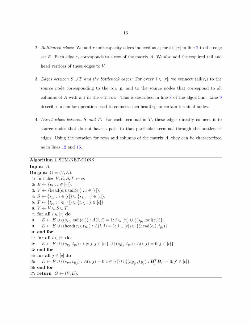
16

2. Bottleneck edges: We add r unit-capacity edges indexed as ei for i ∈ [r] in line 2 to the edge

set E. Each edge ei corresponds to a row of the matrix A. We also add the required tail and

head vertices of these edges to V .

3. Edges between S ∪ T and the bottleneck edges: For every i ∈ [r], we connect tail(ei) to the

source node corresponding to the row pi and to the source nodes that correspond to all

columns of A with a 1 in the i-th row. This is described in line 8 of the algorithm. Line 9

describes a similar operation used to connect each head(ei) to certain terminal nodes.

4. Direct edges between S and T : For each terminal in T , these edges directly connect it to

source nodes that do not have a path to that particular terminal through the bottleneck

edges. Using the notation for rows and columns of the matrix A, they can be characterized

as in lines 12 and 15.

Algorithm 1 SUM-NET-CONS

Input: A.

Output: G = (V,E).

1: Initialize V,E, S, T ← φ.

2: E ← {ei : i ∈ [r]}.3: V ← {head(ei), tail(ei) : i ∈ [r]}.4: S ← {spi : i ∈ [r]} ∪ {sBj : j ∈ [c]}.5: T ← {tpi : i ∈ [r]} ∪ {tBj : j ∈ [c]}.6: V ← V ∪ S ∪ T .

7: for all i ∈ [r] do

8: E ← E ∪ {(sBj , tail(ei)) : A(i, j) = 1; j ∈ [c]} ∪ {(spi , tail(ei))}.9: E ← E ∪ {(head(ei), tBj ) : A(i, j) = 1; j ∈ [c]} ∪ {(head(ei), tpi)}.

10: end for

11: for all i ∈ [r] do

12: E ← E ∪ {(spj , tpi) : i 6= j; j ∈ [r]} ∪ {(sBj , tpi) : A(i, j) = 0; j ∈ [c]}.13: end for

14: for all j ∈ [c] do

15: E ← E ∪ {(spi , tBj ) : A(i, j) = 0; i ∈ [r]} ∪ {(sBj′ , tBj ) : BTj Bj′ = 0; j′ ∈ [c]}.

16: end for

17: return G← (V,E).

17

For an incidence structure I, let AI represent its incidence matrix. The sum-networks con-

structed in the paper are such that the matrix A used in the SUM-NET-CONS algorithm is either

equal to AI or ATI for some incidence structure I. When A = AI , we call the sum-network con-

structed as the normal sum-network for I. Otherwise when A = ATI , we call the sum-network

constructed as the transpose sum-network for I. The following definitions are useful for analysis.

For every p ∈ P, we denote the set of blocks that contain the point p as

〈p〉 := {B ∈ B : p ∈ B}, (2.3)

and for every B ∈ B, the collection of blocks that have a non-empty intersection with B is denoted

by the set

〈B〉 := {B′ ∈ B : B′ ∩B 6= φ} (2.4)

= {B′ ∈ B : BTB′ 6= 0}, (2.5)

where boldface B indicates the column of AI corresponding to block B ∈ B.

The inner product above is computed over the reals. In the sequel, we will occasionally need to

perform operations similar to the inner product over a finite field. This shall be explicitly pointed

out.

We now present some examples of sum-networks constructed using the above technique.

Example 2 Let I be the unique simple line graph on two vertices, with points corresponding to the

vertices and blocks corresponding to the edges of the graph. Denoting the points as natural numbers,

we get that P = {1, 2} and B = {{1, 2}}. Then the associated incidence matrices are as follows.

AI =

1

1

, and ATI =

[1 1

].

Following the SUM-NET-CONS algorithm the two sum-networks obtained are as shown in the

Figure 2.2.

18

s1 s{1,2} s2

t2t{1,2}t1

e2e1

(a)

s1 s{1,2} s2

t{1,2}t1 t2

e{1,2}

(b)

Figure 2.2: Two sum-networks obtained from the line graph on two vertices described in Example2. The source set S and the terminal set T contain three nodes each. All edges are unit-capacityand point downward. The edges with the arrowheads are the bottleneck edges constructed in step2 of the construction procedure. (a) Normal sum-network, and (b) transposed sum-network.

Example 3 In this example we construct a sum-network using a simple t-design. Let I denote

the 2-(3, 2, 1) design with its points denoted by the numbers {1, 2, 3} and its blocks denoted by the

letters {A,B,C}. For this design we have that A = {1, 2}, B = {1, 3}, C = {2, 3} and its associated

incidence matrix under row and column permutations can be written as follows.

AI =

1 1 0

1 0 1

0 1 1

Note that AI = ATI . Hence the normal sum-network and the transposed sum-network are identical

in this case. Following the SUM-NET-CONS algorithm, we obtain the sum-network shown in Figure

2.3.

Remark 1 Note that each edge added in the SUM-NET-CONS algorithm has unit capacity. Propo-

sition 6 in Section 2.7 modifies the SUM-NET-CONS algorithm so that each edge e in the sum-

network has cap(e) = α > 1, α ∈ N.

19

e1

e2

e3

s1 s2 s3

sA sC

sB

t1 t2 t3

tA tC

tB

Figure 2.3: The normal sum-network obtained for the incidence structure I described in Example3. All edges are unit-capacity and directed downward. The edges with the arrowheads are thebottleneck edges, and the edges denoted by dashed lines correspond to the direct edges introducedin step 4 of the construction procedure. For this case, the normal and the transposed sum-networkare identical.

2.5 Upper bound on the computation capacity

In this section, we describe an upper bound on the computation capacity of a sum-network

obtained from a (0, 1)-matrix A of dimension r× c. We assume that there exists a (m,n) fractional

network code assignment, i.e., φe for e ∈ E (and corresponding global encoding functions φe(X))

and decoding functions ψt for t ∈ T so that all the terminals in T can recover the sum of all the

independent sources.

For convenience of presentation, we will change notation slightly and let the messages observed

at the source nodes corresponding to the rows of A as Xpi for i ∈ [r] and those corresponding to

the columns of A as XBj for j ∈ [c]. Each of the messages is a column vector of length m over

F . The set of all source messages is represented by X. We let φe(X) denote the n-length column

vector of symbols from F that are transmitted by the edge e ∈ E, as it is the value returned by the

20

global encoding function φe for edge e on the set of source messages denoted by X. As is apparent,

non-trivial encoding functions can only be employed on the bottleneck edges, i.e., ei for i ∈ [r] as

these are the only edges that have more than one input. For brevity, we denote φi(X) = φei(X).

We define the following set of global encoding functions.

φIn(v)(X) := {φe(X) : e ∈ In(v)}, ∀v ∈ V.

LetH(Y ) be the entropy function for a random variable Y . We let {Yi}l1 denote the set {Y1, Y2, . . . , Yl}

for any l > 1. The following lemma demonstrates that certain partial sums can be computed by

observing subsets of the bottleneck edges.

Lemma 1 If a network code allows each terminal to compute the demanded sum, then the value

X ′pi := Xpi +∑

j:A(i,j)=1XBj can be computed from φi(X), i.e., H(X ′pi |φi(X)

)= 0 for all i ∈ [r].

Similarly for any j ∈ [c] the value X ′Bj :=∑

i:A(i,j)=1Xpi +∑

j′:Bj′∈〈Bj〉XBj′ can be computed from

the set of values {φi(X) : for i ∈ [r], A(i, j) = 1}.

Proof: We let for any i ∈ [r]

Z1 =∑i′ 6=i

Xpi′ , Z2 =∑

j:A(i,j)=1

XBj and Z3 =∑

j:A(i,j)=0

XBj ,

such that the sum Z = Xpi + Z1 + Z2 + Z3 and X ′pi = Xpi + Z2.

By our assumption that each terminal can recover the demanded sum, we know that Z can

be evaluated from φIn(tpi)(X) for all i ∈ [r], i.e., H

(Z|φIn(tpi )

(X))

= 0 for all i ∈ [r]. Since

{Xpi′ : i′ 6= i} and {XBj : A(i, j) = 0} determine the value of Z1 and Z3 respectively and also

determine the values transmitted on each of the direct edges that connect a source node to tpi , we

21

get that

H(Z|φIn(tpi)

(X))

= H(Z|φi(X), {φ(spi′ ,tpi )

(X) : i′ 6= i}, {φ(sBj ,tpi ): A(i, j) = 0}

)(a)

≥ H(Xpi + Z1 + Z2 + Z3|φi(X), {Xpi′ : i′ 6= i}, {XBj : A(i, j) = 0}

)= H

(X ′pi |φi(X), {Xpi′ : i′ 6= i}, {XBj : A(i, j) = 0}

)= H

(X ′pi , {Xpi′ : i′ 6= i}, {XBj : A(i, j) = 0}|φi(X)

)−H

({Xpi′ : i′ 6= i}, {XBj : A(i, j) = 0}|φi(X)

)= H

(X ′pi |φi(X)

)+H

({Xpi′ : i′ 6= i}, {XBj : A(i, j) = 0}|X ′pi , φi(X)

)−H

({Xpi′ : i′ 6= i}, {XBj : A(i, j) = 0}|φi(X)

)(b)= H

(X ′pi |φi(X)

), (2.6)

where inequality (a) follows from the fact that φ(spi′ ,tpi )(X) is a function of Xpi′ for i′ 6= i and

φ(sBj ,tpi )(X) is a function of {XBj : A(i, j) = 0} and equality (b) is due to the fact that X ′pi

is conditionally independent of both {Xpi′ : i′ 6= i} and {XBj : A(i, j) = 0} given φi(X). This

conditional independence can be checked as follows. Let bold lowercase symbols represent specific

realizations of the random variables.

Pr(X ′pi = x′pi , {Xpi′ = xpi′ : i′ 6= i}, {XBj = xBj : A(i, j) = 0}|φi(X) = φi(x)

)(a)=

Pr(X ′pi = x′pi , φi(X) = φi(x)) · Pr({Xpi′ = xpi′ : i′ 6= i}, {XBj = xBj : A(i, j) = 0})Pr(φi(X) = φi(x))

(b)= Pr(X ′pi = x′pi |φi(X) = φi(x)) Pr({Xpi′ = xpi′ : i′ 6= i}, {XBj = xBj : A(i, j) = 0}|φi(X) = φi(x)),

where equalities (a) and (b) are due to the fact that the source messages are independent and φi(x)

is only a function of xpi and the set {xBj : A(i, j) = 1}.

Since terminal tpi can compute Z, H(Z|φIn(tpi)

(X))

= 0 and we get from eq. (2.6) that

H(Xpi + Z2|φi(X)) = 0.

22

For the second part of the lemma, we argue similarly as follows. We let for any j ∈ [c]

Z1 =∑

i:A(i,j)=1

Xpi , Z2 =∑

i:A(i,j)=0

Xpi ,

Z3 =∑

B∈〈Bj〉

XB, Z4 =∑

B/∈〈Bj〉

XB

such that Z = Z1 + Z2 + Z3 + Z4 and X ′Bj = Z1 + Z3. By our assumption, for all j ∈ [c],

H

(Z|φ

In(tBj

)(X)

)= 0. The sets {Xp : p /∈ Bj} and {XB : B /∈ 〈Bj〉} determine the value of

Z2 and Z4 respectively and also the values transmitted on each of the direct edges that connect a

source node to the terminal tBj . Let Φ denote the set {φi(X) : A(i, j) = 1}. Then,

H

(Z|φ

In(tBj

)(X)

)= H

(Z1 + Z2 + Z3 + Z4|Φ, {φ(spi ,tBj )(X) :A(i, j) = 0}, {φ(sB ,tBj ) : B /∈ 〈Bj〉}

)(a)

≥ H (Z1 + Z2 + Z3 + Z4|Φ, {Xpi : A(i, j) = 0}, {XB : B /∈ 〈Bj〉})

= H(X ′Bj |Φ, {Xpi : A(i, j) = 0}, {XB : B /∈ 〈Bj〉}

)= H

(X ′Bj , {Xpi : A(i, j) = 0}, {XB : B /∈ 〈Bj〉}|Φ

)−H ({Xpi : A(i, j) = 0}, {XB : B /∈ 〈Bj〉}|Φ)

= H(X ′Bj |Φ)−H({Xpi :A(i, j) = 0}, {XB :B /∈ 〈Bj〉}|Φ)

+H({Xpi : A(i, j) = 0}, {XB : B /∈ 〈Bj〉}|X ′Bj ,Φ)

(b)= H(X ′Bj |Φ).

Inequality (a) is due to the fact that φ(spi ,tBj )(X) is a function of Xpi and similarly for φ(sB ,tBj )(X).

Equality (b) follows from the fact that Z1 +Z3 is conditionally independent of both {Xpi : A(i, j) =

0} and {XBj′ : B /∈ 〈Bj〉} given the set of random variables {φi(X) : A(i, j) = 1}. This can be

verified in a manner similar to as was done previously. This gives us the result that H(X ′Bj |{φi(X) :

A(i, j) = 1}) = 0.

Next, we show the fact that the messages observed at the source nodes are independent and

uniformly distributed over Fm imply that the random variables X ′pi for all i ∈ [r] are also uniform

i.i.d. over Fm. To do that, we introduce some notation. For a matrix N ∈ Fr×c, for any two

23

index sets R ⊆ [r], C ⊆ [c], we define the submatrix of N containing the rows indexed by R and

the columns indexed by C as N [R, C]. Consider two (0, 1)-matrices N1, N2 of dimensions r1× t and

t× c2 respectively. Here 1 and 0 indicate the multiplicative and additive identities of the finite field

F respectively. The i-th row of N1 is denoted by the row submatrix N1 [i, [t]] ∈ {0, 1}t and the j-th

column of N2 be denoted by the column submatrix N2 [[t], j] ∈ {0, 1}t. Then we define a matrix

function on N1N2 that returns a r1 × c2 matrix (N1N2)# as follows.

(N1N2)#(i, j) =

1,

if the product N1 [i, [t]]N2 [[t], j]

over Z is positive,

0, otherwise.

For an incidence structure I = (P,B) with r×c incidence matrix A, letXp, ∀p ∈ P andXB, ∀B ∈ B

be m-length vectors with each component i.i.d. uniformly distributed over F . We collect all the

independent source random variables in a column vector X having m(r + c) elements from F as

follows

X :=

[XTp1 XT

p2 · · · XTpr XT

B1XTB2· · · XT

Bc

]T.

Recall that pi denotes the i-th row and Bj denotes the j-th column of the matrix A. For all i ∈ [r]

let ei ∈ Fr denote the column vector with 1 in its i-th component and zero elsewhere. Then for

X ′pi , X′Bj

as defined in lemma 1, one can check that (⊗ indicates the Kronecker product of two

matrices)

X′pi =

([eTi pi

]⊗ Im

)X, for all i ∈ [r] and (2.7)

X′Bj =

([BTj (BT

j B1)# . . . (BTj Bc)#

]⊗ Im

)X, (2.8)

for all j ∈ [c] where Im is the identity matrix of size m. By stacking these values in the correct

order, we can get the following matrix equation.[X′Tp1 · · · X

′Tpr X

′TB1· · · X

′TBc

]T= (MA ⊗ Im)X (2.9)

where the matrix MA ∈ F (r+c)×(r+c) is defined as

MA :=

Ir A

AT (ATA)#

. (2.10)

24

Note that the first r rows of MA are linearly independent. There is a natural correspondence

between the rows of MA and the points and blocks of I of which A is the incidence matrix. If

1 ≤ i ≤ r, then the i-th row MA [i, [r + c]] corresponds to the point pi ∈ P and if r+ 1 ≤ j ≤ r+ c,

then the j-th row MA [j, [r + c]] corresponds to the block Bj ∈ B.

Lemma 2 For a (0, 1)-matrix A of size r× c, let X ′pi , X′Bj∈ Fm be as defined in Eqs. (2.7), (2.8)

and matrix MA be as defined in eq. (2.10). Let r + t := rankFMA for some non-negative integer

t and index set S ′ ⊆ {r + 1, r + 2, . . . , r + c} be such that rankFMA [[r] ∪ S ′, [r + c]] = r + t. Let

BS′ := {BS′1 , BS′2 , . . . , BS′t} ⊆ B be the set of blocks that correspond to the rows of MA indexed by

S ′ in increasing order. Then we have

Pr

(X ′p1 = x′1, . . . , X

′pr = x′r, X

′BS′1

= y′1, . . . , X′BS′t

= y′t

)= q−m(r+t), and (2.11)

Pr(X ′pi = x′i

)= Pr

(X ′BS′

j

= y′j

)= q−m, ∀i ∈ [r], j ∈ [t].

Proof: The quantities in the statement of the lemma satisfy the following system of equations

(M[[r] ∪ S ′, [r + c]

]⊗ Im

) [XTp1 · · · XT

pr XTB1· · · XT

Bc

]T=

[X′Tp1 · · · X

′Tpr X

′TBS′1

· · · X′TBS′t

]T.

The vector

[XTp1 · · · XT

pr XTB1· · · XT

Bc

]Tis uniform over Fm(r+c). Since the matrix

M [[r] ∪ S ′, [r + c]] ⊗ Im has full row rank equal to m(r + t), the R.H.S. of the above equation is

uniformly distributed over Fm(r+t), giving the first statement. The second statement is true by

marginalization.

Theorem 1 The computation capacity of any sum-network constructed by the SUM-NET-CONS

algorithm is at most 1.

Proof: By the construction procedure, there is a terminal tpi which is connected to the

sources spi and {sBj : A(i, j) = 1} through the edge ei. By lemmas 1 and 2 we have thatH(φi(X)) ≥

m log2 q bits. From the definition of n the maximum amount of information transmitted on ei is

n log2 q bits and that implies that m ≤ n.

25

Next, we show that the upper bound on the computation capacity exhibits a strong dependence on

the characteristic of the field (denoted ch(F)) over which the computation takes place.

Theorem 2 Let A be a (0, 1)-matrix of dimension r × c and suppose that we construct a sum-

network corresponding to A using the SUM-NET-CONS algorithm. The matrix MA is as defined

in eq. (2.10). If rankFMA = r + t, the upper bound on computation capacity of the sum-network

is r/(r + t).

Proof: Let BS′ ⊆ B be as defined in lemma 2. Then from lemmas 1 and 2, we have

H(X ′pi |φi(X)

)= 0, ∀i ∈ [r] and H

(X ′BS′

j

|{φi(X) : A(i, j) = 1})

= 0, ∀j ∈ [t]. Hence we have

that H({φi(X)}r1) ≥ m(r + t) log q. From the definition of n, we get nr log q ≥ H({φi(X)}r1) ≥

m(r + t) log q =⇒ m/n ≤ r/(r + t).

Proposition 1 We have that rankFMA = r + t if and only if rankF((ATA)# −ATA

)= t. Fur-

thermore, rankFMA = r + c if and only if ch(F) - detZMA, where detZ indicates the determinant

of the matrix with its elements interpreted as 0 or 1 in Z.

Proof: From eq. (2.10), we have that

MA=

Ir A

AT (ATA)#

=

Ir 0

AT Ic

Ir 0

0 (ATA)# −ATA

Ir A

0 Ic

, (2.12)

which gives us the rank condition. Since MA is a (0, 1)-matrix, if it has full rank, then its deter-

minant is some non-zero element of F , where F is the base subfield of F having prime order. We

could also interpret the elements of MA as integers and evaluate its determinant detZMA. Then if

MA has full rank, we have that ch(F) - detZMA.

Example 4 Consider the normal sum-network obtained from using the Fano plane for which

the incidence matrix AI is as defined in eq. (2.1), so that r = c = 7. It can be verified that

rankGF (2)MAI = 7. Hence theorem 2 gives an upper bound of 1 for the computation capacity. In

fact, there is a rate-1 network code that satisfies all terminals in the normal sum-network obtained

using the Fano plane as described later in proposition 4.

26

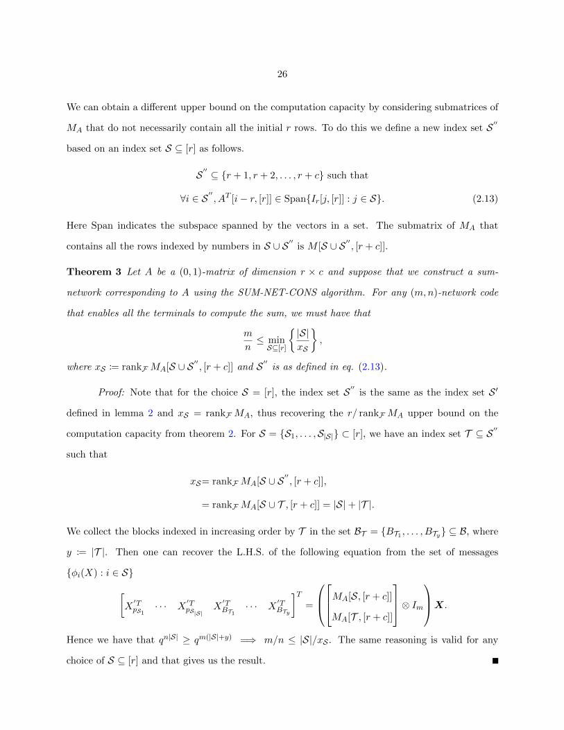
We can obtain a different upper bound on the computation capacity by considering submatrices of

MA that do not necessarily contain all the initial r rows. To do this we define a new index set S ′′

based on an index set S ⊆ [r] as follows.

S ′′ ⊆ {r + 1, r + 2, . . . , r + c} such that

∀i ∈ S ′′ , AT [i− r, [r]] ∈ Span{Ir[j, [r]] : j ∈ S}. (2.13)

Here Span indicates the subspace spanned by the vectors in a set. The submatrix of MA that

contains all the rows indexed by numbers in S ∪ S ′′ is M [S ∪ S ′′ , [r + c]].

Theorem 3 Let A be a (0, 1)-matrix of dimension r × c and suppose that we construct a sum-

network corresponding to A using the SUM-NET-CONS algorithm. For any (m,n)-network code

that enables all the terminals to compute the sum, we must have that

m

n≤ minS⊆[r]

{ |S|xS

},

where xS := rankFMA[S ∪ S ′′ , [r + c]] and S ′′ is as defined in eq. (2.13).

Proof: Note that for the choice S = [r], the index set S ′′ is the same as the index set S ′

defined in lemma 2 and xS = rankFMA, thus recovering the r/ rankFMA upper bound on the

computation capacity from theorem 2. For S = {S1, . . . ,S|S|} ⊂ [r], we have an index set T ⊆ S ′′

such that

xS= rankFMA[S ∪ S ′′ , [r + c]],

= rankFMA[S ∪ T , [r + c]] = |S|+ |T |.

We collect the blocks indexed in increasing order by T in the set BT = {BT1 , . . . , BTy} ⊆ B, where

y := |T |. Then one can recover the L.H.S. of the following equation from the set of messages

{φi(X) : i ∈ S}[X′TpS1

· · · X′TpS|S|

X′TBT1

· · · X′TBTy

]T=

MA[S, [r + c]]

MA[T , [r + c]]

⊗ ImX.

Hence we have that qn|S| ≥ qm(|S|+y) =⇒ m/n ≤ |S|/xS . The same reasoning is valid for any

choice of S ⊆ [r] and that gives us the result.

27

1

4

23

5 6

AB

CD

C

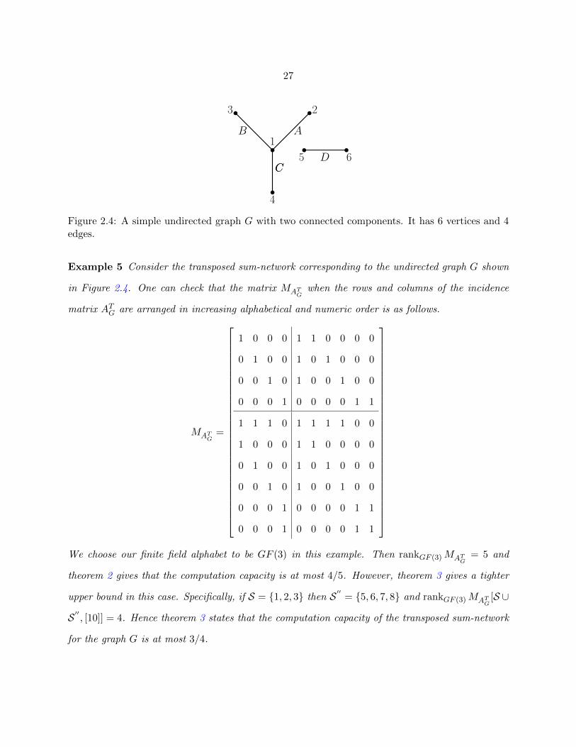
Figure 2.4: A simple undirected graph G with two connected components. It has 6 vertices and 4edges.

Example 5 Consider the transposed sum-network corresponding to the undirected graph G shown

in Figure 2.4. One can check that the matrix MATGwhen the rows and columns of the incidence

matrix ATG are arranged in increasing alphabetical and numeric order is as follows.

MATG=

1 0 0 0 1 1 0 0 0 0

0 1 0 0 1 0 1 0 0 0

0 0 1 0 1 0 0 1 0 0

0 0 0 1 0 0 0 0 1 1

1 1 1 0 1 1 1 1 0 0

1 0 0 0 1 1 0 0 0 0

0 1 0 0 1 0 1 0 0 0

0 0 1 0 1 0 0 1 0 0

0 0 0 1 0 0 0 0 1 1

0 0 0 1 0 0 0 0 1 1

We choose our finite field alphabet to be GF (3) in this example. Then rankGF (3)MATG

= 5 and

theorem 2 gives that the computation capacity is at most 4/5. However, theorem 3 gives a tighter

upper bound in this case. Specifically, if S = {1, 2, 3} then S ′′ = {5, 6, 7, 8} and rankGF (3)MATG[S ∪

S ′′ , [10]] = 4. Hence theorem 3 states that the computation capacity of the transposed sum-network

for the graph G is at most 3/4.

28

We apply the above theorems to obtain characteristic dependent upper bounds on the computation

capacity of some infinite families of sum-networks constructed using the given procedure.

Corollary 1 Let I = (P,B) be an incidence structure obtained from a simple undirected graph

where P denotes the set of vertices and B consists of the 2-subsets of P corresponding to the edges.

Let deg(p) ∈ Z represent the degree of vertex p ∈ P. The incidence matrix AI has dimension

|P| × |B|. The computation capacity of the normal sum-network constructed using AI is at most

|P||P|+|B| for any finite field F .

Let F be the finite field alphabet of operation and define P ′ ⊆ P as P ′ := {p : ch(F) - (deg(p)−

1), p ∈ P}. Consider the set of edges B′ := ∪p∈P ′〈p〉. The computation capacity of the transposed

sum-network is at most |B′||B′|+|P ′| .

Proof: Recall that BTi is the i-th row of ATI for all i ∈ [|B|]. Then the inner product over F

between two rows is

BTi Bj =

2 (mod ch(F)), if i = j,

1,if edges indexed by i and

j have a common vertex,

0, otherwise.

It can be observed that the matrix of interest, i.e., (ATIAI)# − ATIAI = −I|B| has full rank over

every finite field.

The transposed sum-network for I is obtained by applying the SUM-NET-CONS algorithm on

the |B| × |P| matrix ATI , so that the parameters r = |B|, c = |P|. We apply theorem 3 by choosing

the index set S ⊆ [|B|] such that S = {j : Bj ∈ B′}. Defined this way, |S| = |B′| and S ′′ is obtained

from S using eq. (2.13). We collect all the points corresponding to the rows in the submatrix

MATI[S ′′ , [r + c]] in a set PS′′ ⊆ P. Note that PS′′ depends on the set of edges B′. By definitions

of B′ and S ′′ , we have that P ′ ⊆ PS′′ . This is true because B′ consists of all the edges that are

incident to at least one point in P ′ while indices in the set S ′′ correspond to all points that are not

incident to any edge outside B′. For instance, in Example 5 above, as F = GF (3), P ′ = {1}. Then

B′ = {A,B,C} and PS′′ = {1, 2, 3, 4}.

29

We now show that rankFMA[S ∪ S ′′ ] = |B′| + |P ′| and that gives us the result using theorem

3. Recall that pi denotes the i-th row of AI , which corresponds to the vertex pi for all i ∈ [|P|]. It

follows that the inner product between pi,pj over F is

pipTj =

deg(pi) (mod ch(F)), if i = j,

1, if {i, j} ∈ B,

0, otherwise.

Because of the above equation, all the off-diagonal terms in the matrix (AIATI )# − AIA

TI are

equal to zero. We focus on the submatrix M [S ∪ S ′′ , [r + c]] obtained from eq. (2.12), letting

S ′′|B| = {j − |B| : j ∈ S′′} we get that

M [S ∪ S ′′ , [r + c]] =

I|B|[S,S] 0

AI [S′′

|B|,S] I|P|

[S ′′|B|,S

′′

|B|

] · Λ ·

I|B| ATI

0 I|P|

,where

Λ :=

I|B|[S, [|B|]] 0

0((AIA

TI )# −AIATI

) [S ′′|B|, [|P|]

] .

By definition of P ′ the points in the set PS′′ \ P ′ are such that deg(pi) − 1 ≡ 0 (mod ch(F)),

i.e., the diagonal entry corresponding to those points in (AIATI )# −AIATI in the matrix Λ is zero.

Thus, Λ has exactly |B′| + |P ′| rows which are not equal to the all-zero row vector. The first and

third matrices are invertible, and hence we get that rankFMA[S ∪ S ′′ , [r + c]] = |B′|+ |P ′|.

Corollary 2 Let I = (P,B) be a 2-(v, k, 1) design. For the normal sum-network constructed using

the |P| × |B| incidence matrix AI , the computation capacity is at most |P||P|+|B| if ch(F) - (k − 1).

For the transposed sum-network constructed using ATI , the computation capacity is at most |B||P|+|B|

if ch(F) - v−kk−1 .

Proof: We first describe the case of the transposed sum-network. From eq. (2.2) each point

in a 2-(v, k, 1) design is incident to ρ = v−1k−1 blocks. Moreover any two points occur together in

30

exactly one block. Thus, we have the inner product over F as

pipTj =

v−1k−1 (mod ch(F)), if j = i,

1, otherwise.

This implies that AIATI − (AIA

TI )# =

[(v−1k−1 − 1

)]Iv =

[v−kk−1

]Iv and setting its determinant

non-zero gives the result.

For the normal sum-network, we argue as follows. Note that BTi Bi = k (mod ch(F)) for any

i. Since any two points determine a unique block, two blocks can either have one point or none in

common. Hence, for i 6= j, the inner product over F is

BTi Bj =

1, if Bi ∩Bj 6= ∅,

0, otherwise.

Then ATIAI − (ATIAI)# = [(k − 1)] Ib and setting its determinant as non-zero gives the result.

Corollary 3 Let I = (P,B) be a t-(v, k, λ) design, for t ≥ 2. From eq. (2.2), each point is present

in ρ := λ(v−1t−1

)/(k−1t−1

)blocks and the number of blocks incident to any pair of points is given by

b2 := λ(v−2t−2

)/(k−2t−2

). Consider the transposed sum-network constructed using the incidence matrix

ATI which has dimension |B| × |P|. The computation capacity of the transposed sum-network is at

most |B||B|+|P| if

ch(F) - [ρ− b2 + v(b2 − 1)](ρ− b2)v−1.

Proof: By definition, we have that the inner product over F between two rows is

pipTj =

ρ (mod ch(F)), if j = i,

b2 (mod ch(F)), otherwise.

It follows that AIATI − (AIA

TI )# has the value (ρ − 1) on the diagonal and (b2 − 1) elsewhere.

Hence

AIATI − (AIA

TI )# = [(ρ− b2) (mod ch(F))] Iv + [(b2 − 1) (mod ch(F))] Jv,

31

where Jv denotes the square all ones matrix of dimension v. Then by elementary row and columns

operations, det[AIA

TI − (AIA

TI )#

]can be evaluated to be equal to [ρ− b2 + v(b2 − 1)](ρ− b2)v−1

(mod ch(F)).

Corollary 4 Let D = (P,B) be a t-(v, t + 1, λ) design with λ 6= 1 and incidence matrix AD. We

define a higher incidence matrix AD′ of dimension(|P|t

)× |B| such that each row corresponds to a

distinct t-subset of P and each column corresponds to a block in B. AD′ is a (0, 1)-matrix such that

for any i ∈[(vt

)], j ∈ [|B|], its entry AD′(i, j) = 1 if each of the points in the t-subset corresponding

to the i-th row is incident to the block Bj ∈ B and zero otherwise. The computation capacity

of the normal sum-network constructed using AD′ is at most(vt)

(vt)+|B| = t+1λ+t+1 if ch(F) - t. The

computation capacity of the transposed sum-network constructed using ATD′ is at most |B||B|+(vt)

=

λλ+t+1 if ch(F) - (λ− 1).

Proof: The incidence matrix AD′ is a (0, 1) matrix of dimension(vt

)× λ

t+1

(vt

). Let pi,Bu

denote the i-th row and u-th column respectively of AD′ for i ∈[(vt

)], u ∈

[λt+1

(vt

)]. Each row of

AD′ corresponds to a distinct t-subset of P. By t-design criterion, any set of t points belongs to

exactly λ blocks. Since the columns have a one-to-one correspondence with the blocks in B, each

row of AD′ has exactly λ 1’s. Two rows will have a 1 in the same column if the block corresponding

to the column is incident to both the t-subsets corresponding to the two rows. Since each block

has t + 1 points, there cannot be more than one block incident to two different t-subsets. Hence,

for the inner product over F , we have that pipTi = λ (mod ch(F)) and for all i 6= j; i, j,∈

[(vt

)],

pipTj =

1,

if the union of the t-subsets corresponding to

the i-th and j-th rows is a block in B,

0, otherwise.

Then AD′ATD′−(AD′A

TD′)# = [(λ− 1) (mod ch(F))] I(vt)

and that gives the result for the transposed

sum-network.

For the normal sum-network, we look at the columns of AD′ in a similar manner. Each column

of AD′ corresponds to a block in B. Since the size of each block is t + 1, each column has exactly

32

(t+1t

)= t + 1 elements as 1. Also, two different blocks can have at most t points in common, and

only when that happens, will the two columns have a 1 in the same row. Hence, for the inner

product over F , we have that BTuBu = (t+ 1) (mod ch(F)) and for all u 6= v;u, v ∈

[(vt

)],

BTuBv =

1,

if the u-th and v-th blocks have t points

in common,

0, otherwise.

Then ATD′AD′ − (ATD′AD′)# = t (mod ch(F))I λt+1(vt)

and theorem 2 gives the result.

2.6 Linear network codes for constructed sum-networks

In this section, we propose linear network codes for the sum-networks constructed using the

SUM-NET-CONS algorithm. Recall that the algorithm takes a (0, 1)-matrix A that has r rows

and c columns as its input. In Section 2.5, we demonstrated that the incidence matrix of certain

incidence structures result in sum-networks whose capacity can be upper bounded (cf. Corollaries

1, 2, 4). We now demonstrate that under certain conditions, we can obtain network codes whose

rate matches the corresponding upper bound. Thus, we are able to characterize the capacity of a

large family of sum-networks.

We emphasize that random linear network codes that have been used widely in the literature

for multicast code constructions are not applicable in our context. In particular, it is not too hard

to argue that a random linear network code would result in each terminal obtaining a different

linear function or subspace. Thus, constructing codes for these sum-networks requires newer ideas.

We outline the key ideas by means of the following example.

Example 6 Consider the sum-network shown in Figure 2.2a. The matrix AI used in its construc-

tion is of dimension r× c where r = 2, c = 1 and is described in Example 2. It can be observed that

ATIAI −(ATIAI

)#

= 1. Then theorem 2 states that the computation capacity of this sum-network

is at most 2/3. We describe a network code with m = 2, n = 3. The global encoding functions

for the two bottleneck edges are shown in Table 2.1. Using the values transmitted, all three

terminals can recover the sum in the following manner. t1 receives the value of X2 from the direct

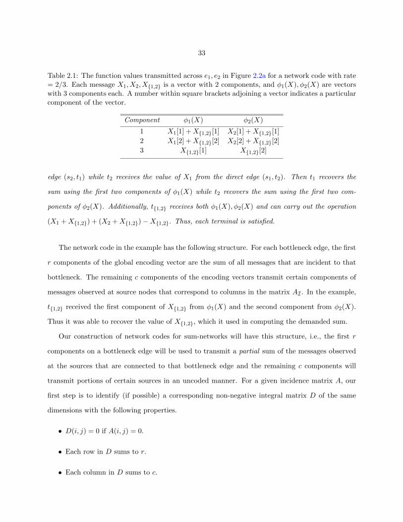
33

Table 2.1: The function values transmitted across e1, e2 in Figure 2.2a for a network code with rate= 2/3. Each message X1, X2, X{1,2} is a vector with 2 components, and φ1(X), φ2(X) are vectorswith 3 components each. A number within square brackets adjoining a vector indicates a particularcomponent of the vector.

Component φ1(X) φ2(X)

1 X1[1] +X{1,2}[1] X2[1] +X{1,2}[1]

2 X1[2] +X{1,2}[2] X2[2] +X{1,2}[2]

3 X{1,2}[1] X{1,2}[2]

edge (s2, t1) while t2 receives the value of X1 from the direct edge (s1, t2). Then t1 recovers the

sum using the first two components of φ1(X) while t2 recovers the sum using the first two com-

ponents of φ2(X). Additionally, t{1,2} receives both φ1(X), φ2(X) and can carry out the operation

(X1 +X{1,2}) + (X2 +X{1,2})−X{1,2}. Thus, each terminal is satisfied.

The network code in the example has the following structure. For each bottleneck edge, the first

r components of the global encoding vector are the sum of all messages that are incident to that

bottleneck. The remaining c components of the encoding vectors transmit certain components of

messages observed at source nodes that correspond to columns in the matrix AI . In the example,

t{1,2} received the first component of X{1,2} from φ1(X) and the second component from φ2(X).

Thus it was able to recover the value of X{1,2}, which it used in computing the demanded sum.

Our construction of network codes for sum-networks will have this structure, i.e., the first r

components on a bottleneck edge will be used to transmit a partial sum of the messages observed

at the sources that are connected to that bottleneck edge and the remaining c components will

transmit portions of certain sources in an uncoded manner. For a given incidence matrix A, our

first step is to identify (if possible) a corresponding non-negative integral matrix D of the same

dimensions with the following properties.

• D(i, j) = 0 if A(i, j) = 0.

• Each row in D sums to r.

• Each column in D sums to c.

34

Under certain conditions on the incidence matrix A, we will show that D can be used to construct

suitable network codes for the sum-networks under consideration.

The existence of our proposed network codes are thus intimately related to the existence of non-

negative integral matrices that satisfy certain constraints. The following theorem [33, Corollary

1.4.2] is a special case of a more general theorem in [34] that gives the necessary and sufficient

conditions for the existence of non-negative integral matrices with constraints on their row and

column sums. We give the proof here since we use some ideas from it in the eventual network code

assignment.

Theorem 4 Let R = (r1, r2, . . . , rm) and S = (s1, s2, . . . , sn) be non-negative integral vectors

satisfying r1 + . . .+ rm = s1 + . . .+ sn. There exists an m× n nonnegative integral matrix D such

that

0 ≤ D(i, j) ≤ cij , ∀i ∈ [m], ∀j ∈ [n],n∑j=1

D(i, j) = ri, ∀i ∈ [m], and

m∑i=1

D(i, j) = sj , ∀j ∈ [n]

if and only if for all I ⊆ [m] and J ⊆ [n], we have that

∑i∈I

∑j∈J

cij ≥∑j∈J

sj −∑i/∈I

ri. (2.14)

Proof: Consider a capacity-limited flow-network modelled using a bipartite graph on m+ n

nodes. The left part has m nodes denoted as xi, ∀i ∈ [m] and the right part has n nodes denoted as

yj ,∀j ∈ [n]. For all i, j there is a directed edge (xi, yj) with capacity cij . There are two additional

nodes in the flow-network, the source node S∗ and terminal node T ∗. There are directed edges

(S∗, xi) with capacity ri for all i ∈ [m] and directed edges (yj , T∗) with capacity sj for all j ∈ [n].

Let xI be the set of all nodes in the left part whose indices are in I and let yJ be the set of all nodes

in the right part whose indices are not in J . Consider a cut separating nodes in {S∗} ∪ xI ∪ yJfrom its complement. Let f∗ be the value of the maximum S∗-T ∗ flow in this network. Then we

35

must have that for all possible choice of subsets I ⊆ [m], J ⊆ [n],

∑i/∈I

ri +∑

(i,j):i∈I,j∈J

cij +∑j /∈J

sj ≥ f∗. (2.15)

In particular, suppose that f∗ =∑

j∈[n] sj in the flow-network. Substituting this in eq. (2.15), we

get the condition that for all possible subsets I ⊆ [m], J ⊆ [n],

∑i∈I

∑j∈J

cij ≥∑j∈J

sj −∑i/∈I

ri. (2.16)

Note that by choosing all possible subsets I, J , we are considering every possible S∗-T ∗ cut in the

network. Then by the maxflow-mincut theorem, the set of conditions of the form of eq. (2.16) for

all I, J are not only necessary but also sufficient for the existence of a flow of value f∗ =∑

j∈[n] sj

in the network.

A feasible flow with this value can be used to arrive at the matrix D as follows. We set the value

of element D(i, j) in the matrix to be equal to the value of the feasible flow on the edge (xi, yj) for

all i ∈ [m], j ∈ [n]. It is easy to verify that the matrix D satisfies the required conditions.

Using the existence theorem for nonnegative integral matrices, we can obtain network codes for

sum-networks constructed from certain incidence structures. The following theorem describes a set

of sufficient conditions that, if satisfied by an incidence structure, allow us to construct a linear

network code that has the same rate as the computation capacity of that sum-network. The proof

of the theorem is constructive and results in an explicit network code.

Theorem 5 Let I = (P,B) be an incidence structure and let AI denote the corresponding inci-

dence matrix of dimension v × b. Suppose that the following conditions are satisfied.

• ATIAI−(ATIAI)# = diag(µ1, . . . , µb) (mod ch(F)), where µi is a non-zero element of F ∀i ∈

{1, 2, . . . , b}.

36

• There exists a matrix DI with integer elements of the same dimension as AI whose entries

satisfy

DI(i, j) = 0, if AI(i, j) = 0, (2.17)

v∑i=1

DI(i, j) = v, and (2.18)

b∑j=1

DI(i, j) = b. (2.19)

Then the computation capacity of the sum-network constructed using AI via the SUM-NET-CONS al-

gorithm is vv+b . This rate can be achieved by a linear network code.

Proof: Note that ATIAI − (ATIAI)# has full rank by assumption, theorem 2 states that

the computation capacity of the sum-network is at most v/(v + b). We construct a (m,n) linear

network code with m = v, n = v + b using the matrix DI . Since m = v, each message vector has v

components. For a vector t ∈ Fv, the notation t[l1 : l2] for two positive integers l1, l2 ∈ [v] denotes a

(l2− l1 +1) length vector that contains the components of t with indices in the set {l1, l1 +1, . . . , l2}

in order. We need to specify the global encoding vectors φi(X) only for the bottleneck edges

ei, i ∈ [v] as all the other edges in the network act as repeaters. The linear network code is such

that the first v components of the vector transmitted along ei ∀i ∈ [v] is

φi(X)[1 : v] = Xpi +∑

j:AI(i,j)=1

XBj .

By construction, each tpi∀i ∈ [v] is connected to the source nodes in {spi′ : i′ 6= i}∪{sBj : AI(i, j) =

0} by direct edges. tpi can then compute the following value from the information received on the

direct edges. ∑i′ 6=i

Xpi +∑

j:AI(i,j)=0

XBj .

Adding the above value to φi(X)[1 : v] enables tpi to compute the required sum. In what follows,

we focus on terminals of the form tBj∀j ∈ [b].

37

Since n = v+ b, each vector φi(X) ∈ Fn has b components that haven’t been specified yet. We

describe a particular assignment for the b components on every φi(X), i ∈ [v] using the matrix DI

that enables each tBj∀j ∈ [b] to compute the sum.

Recall the bipartite flow network constructed in the proof of theorem 4. The nodes in the left

part are denoted as pi∀i ∈ [v] and the nodes in the right part are denoted as Bj∀j ∈ [b]. There is

an edge (pi, Bj) if and only if AI(i, j) = 1. The flow on the edge (pi, Bj) is denoted as f(pi, Bj)

and its value is determined by DI(i, j), i.e., f(pi, Bj) := DI(i, j).

By constraints on the row and column sums ofDI , we conclude that the value of the flow through

any pi∀i ∈ [v] is b and the value of the flow through any Bj∀j ∈ [b] is v. Without loss of generality,

assume that Bj = {p1, p2, · · · , p|Bj |}. We can partition the v components of message vector XBj

into |Bj | parts such that the i-th partition contains f(pi, Bj) distinct components of XBj . Such

a partitioning can be done for all message vectors XBj , j ∈ [b]. Then the flow f(pi, Bj) indicates

that the vector φi(X)[v+ 1 : v+ b] includes f(pi, Bj) uncoded components of XBj . Assigning such

an interpretation to every edge in the flow-network is possible as the total number of components

available in each φi(X) is b and that is also equal to the flow through the point pi.

By construction, terminal tBj is connected to all bottleneck edges in the set {ei : AI(i, j) = 1}.

From the assignment based on the flow, tBj receives f(pi, Bj) distinct components of XBj from

φi(X) for all {i : AI(i, j) = 1}. Since∑v

i=1 f(pi, Bj) = v, it can recover all v components of XBj

in a piecewise fashion.

By adding the first v components transmitted on all the bottleneck edges that are connected to

tBj , it can recover

∑i:AI(i,j)=1

φi(X)[1 : v]

=∑

i:AI(i,j)=1

Xpi +∑

i:AI(i,j)=1

∑l:AI(i,l)=1

XBl ,

=∑

i:AI(i,j)=1

Xpi +∑

Bl∈〈Bj〉

BTj BlXBl .

38

Because of the condition that ATIAI − (ATIAI)# = diag(µ1, µ2, . . . , µb), one can verify that

∑Bl∈〈Bj〉

BTj BlXBl = (µj + 1)XBj +

∑Bl∈〈Bj〉\Bj

XBl .

By the flow-based assignment, each tBj obtains the value of XBj in a piecewise manner. It can

then carry out the following

∑i:AI(i,j)=1

φi(X)[1 : v]− µjXBj

=∑

i:AI(i,j)=1

Xpi + (µj + 1)XBj +∑

Bl∈〈Bj〉\Bj

XBl − µjXBj ,

=∑p∈Bj

Xp +∑

Bl∈〈Bj〉

XBl .

The messages not present in this partial sum, i.e., {Xp : p /∈ Bj} ∪ {XB : B /∈ 〈Bj〉} are available

at tBj through direct edges by construction. Hence, terminals that correspond to a column of AI

are also able to compute the required sum.

We illustrate the linear network code proposed above by means of the following example.

Example 7 Consider the normal sum-network obtained from the undirected simple graph G shown

in Figure 2.5a. A part of the sum-network is shown in Figure 2.5b. The 4 × 5 incidence matrix

AG satisfies the condition of theorem 4 and therefore has an associated matrix DG with row-sum

as 5 and column-sum 4 as shown below. The rows and columns of AG are arranged in increasing

numeric and alphabetical order.

AG =

1 0 0 1 1

1 1 0 0 0

0 1 1 0 1

0 0 1 1 0

, DG =

2 0 0 2 1

2 3 0 0 0

0 1 1 0 3

0 0 3 2 0

.

Using the matrix DG, one can construct a structured linear network code with rate = v/(v+b) = 4/9

as shown in Table 2.2. One can check that it enables all the terminals to compute the required sum.

The flow-network corresponding to DG is shown in Figure 2.5c, and the messages corresponding to

the flow on the solid edges are shown alongside the respective edge.

39

1

2 3

4

A

B

C

D

E

(a)

sA sB sC

sDsE

tA tB tC

tDtE

e1 e2 e3 e4

(b)

XA[1 : 2]XA[3 : 4]

XE[1]

XD[1 : 2]

1

2

3

4

A

B

C

D

E

(c)

Figure 2.5: (a) Undirected graph considered in Example 7. (b) Part of the corresponding normalsum-network constructed for the undirected graph in (a). The full normal sum-network has ninenodes each in the source set S and the terminal set T . However, for clarity, only the five sourcesand terminals that correspond to the columns of the incidence matrix of the graph are shown.Also, the direct edges constructed in Step 4 of the construction procedure are not shown. All edgesare unit-capacity and point downward. The edges with the arrowheads are the bottleneck edgesconstructed in step 2 of the construction procedure. (c) Bipartite flow network as constructed inthe proof of theorem 4 for this sum-network. The message values corresponding to the flow on thesolid lines are also shown.

We can also consider the transposed sum-network for the same graph G. Corollary 1 gives

an upper bound on the computation capacity that depends on F . If F = GF (2), then the subset

of points P ′ = {2, 4} and the upper bound is 4/6. Note that theorem 5 is not applicable here as

the matrix ATGAG − (ATGAG)# does not have all its diagonal elements as non-zero over GF (2).

Proposition 3 gives a condition for the existence of a network code for transposed sum-networks

obtained using irregular graphs. We apply that condition to the transposed sum-network of the

graph G considered here in Example 8.

In the following proposition we show that certain infinite families of incidence structures satisfy the

requirements stated in theorem 5. In particular, the incidence structures considered in Corollaries

1, 2 and 4 satisfy the conditions and hence the computation capacity of the associated sum-networks

can be calculated.

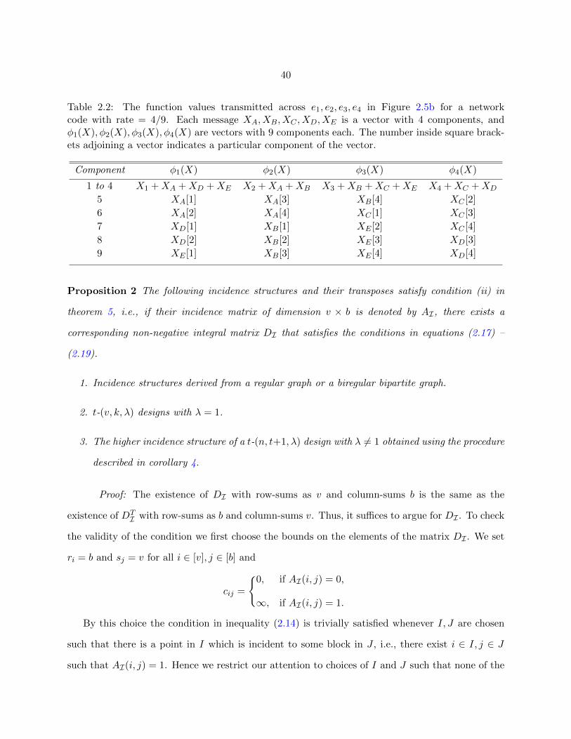
40

Table 2.2: The function values transmitted across e1, e2, e3, e4 in Figure 2.5b for a networkcode with rate = 4/9. Each message XA, XB, XC , XD, XE is a vector with 4 components, andφ1(X), φ2(X), φ3(X), φ4(X) are vectors with 9 components each. The number inside square brack-ets adjoining a vector indicates a particular component of the vector.

Component φ1(X) φ2(X) φ3(X) φ4(X)

1 to 4 X1 +XA +XD +XE X2 +XA +XB X3 +XB +XC +XE X4 +XC +XD

5 XA[1] XA[3] XB[4] XC [2]

6 XA[2] XA[4] XC [1] XC [3]

7 XD[1] XB[1] XE [2] XC [4]

8 XD[2] XB[2] XE [3] XD[3]

9 XE [1] XB[3] XE [4] XD[4]

Proposition 2 The following incidence structures and their transposes satisfy condition (ii) in

theorem 5, i.e., if their incidence matrix of dimension v × b is denoted by AI , there exists a

corresponding non-negative integral matrix DI that satisfies the conditions in equations (2.17) –

(2.19).

1. Incidence structures derived from a regular graph or a biregular bipartite graph.

2. t-(v, k, λ) designs with λ = 1.

3. The higher incidence structure of a t-(n, t+1, λ) design with λ 6= 1 obtained using the procedure

described in corollary 4.

Proof: The existence of DI with row-sums as v and column-sums b is the same as the

existence of DTI with row-sums as b and column-sums v. Thus, it suffices to argue for DI . To check

the validity of the condition we first choose the bounds on the elements of the matrix DI . We set

ri = b and sj = v for all i ∈ [v], j ∈ [b] and

cij =

{0, if AI(i, j) = 0,

∞, if AI(i, j) = 1.

By this choice the condition in inequality (2.14) is trivially satisfied whenever I, J are chosen

such that there is a point in I which is incident to some block in J , i.e., there exist i ∈ I, j ∈ J

such that AI(i, j) = 1. Hence we restrict our attention to choices of I and J such that none of the

41

points in I are incident to any block in J . Under this restriction, the L.H.S. of inequality (2.14) is

0 and the condition is equivalent to (v − |I|)b ≥ |J |v. We will assume that

∃I ⊆ [v], J ⊆ [b] such that (2.20)

AI(i, j) = 0 ∀i ∈ I, j ∈ J, and (v − |I|)b < |J |v,

and show that it leads to a contradiction for each of the three incidence structures considered.

If I corresponds to a d-regular simple graph, then b = dv/2. Consider the point-block incidence

matrix AI , which is a (0, 1)-matrix of size v × b. For the chosen I in eq. (2.20), we look at the

submatrix AI [I, [b]] of size |I| × b that consists of the rows of AI indexed by the points in I and

all the columns. Let l1 be the number of columns with a single 1 in AI [I, [b]] and l2 be the number

of columns with two 1s in AI [I, [b]]. By counting the total number of 1s in AI [I, [b]] in two ways,

we get that

d|I| = l1 + 2l2 ≤ 2(l1 + l2) =⇒ l1 + l2 ≥d|I|2.

Since the number of edges incident to at least one point in I is l1 + l2, any subset J of the edges

that has no incidence with any point in I satisfies |J | ≤ b − d|I|/2. Using these in eq. (2.20) we

get that

(v − |I|)b < |J |v =⇒ (v − |I|)dv2<

(dv

2− d|I|

2

)v,

which is a contradiction.

Now suppose that I corresponds to a biregular bipartite graph, with L vertices having degree dL

in the left part and R vertices having degree dR in the right part. Then b = LdL = RdR. Consider

a subset IL ∪ IR of its vertices. Let EL (resp. ER) be the set of edges which are incident to some

vertex in IL (resp. IR) but not incident to any vertex in IR (resp. IL). The number of edges that

are not incident to any vertex in IL ∪ IR is equal to (L − |IL|)dL − |ER| = (R − |IR|)dR − |EL|.

Suppose there is a choice of I in eq. (2.20) is such that I = IL ∪ IR for some IL, IR. Then we have

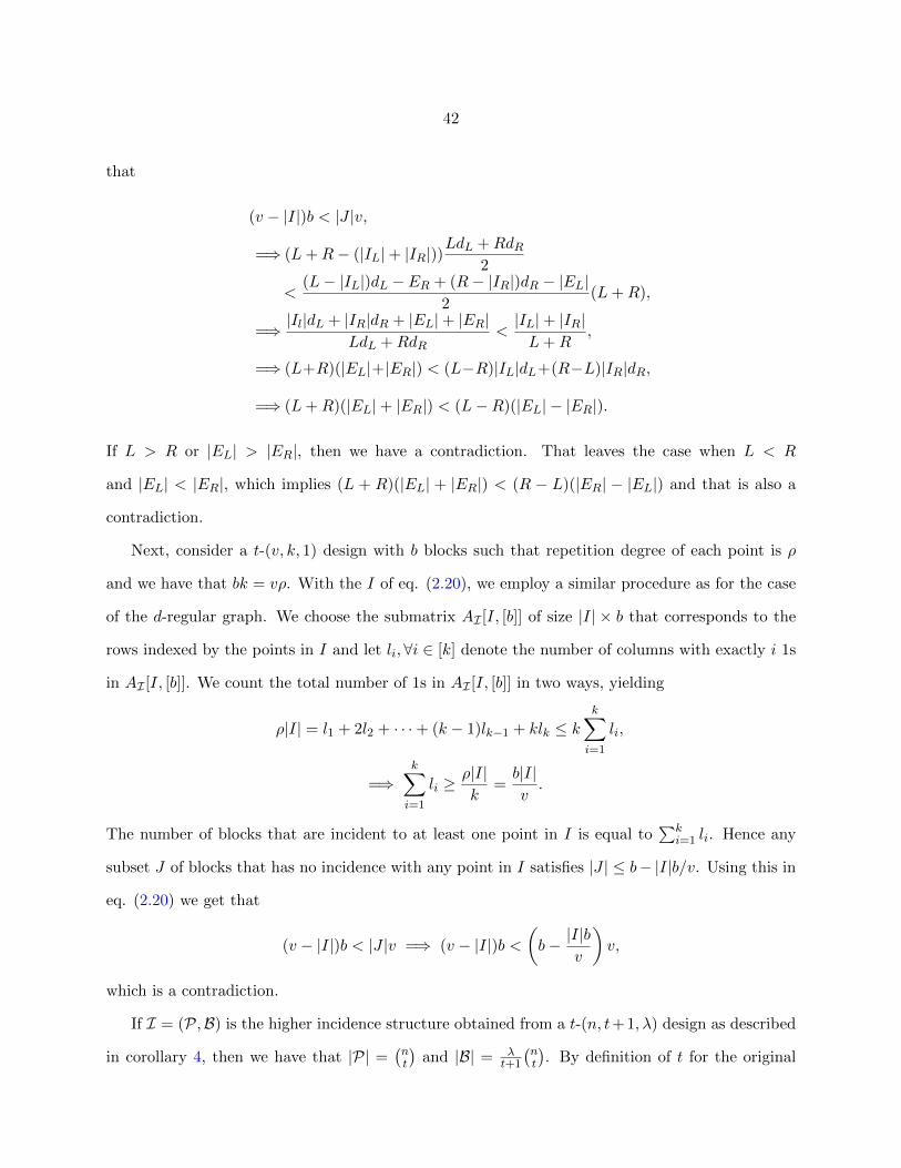
42

that

(v − |I|)b < |J |v,

=⇒ (L+R− (|IL|+ |IR|))LdL +RdR

2

<(L− |IL|)dL − ER + (R− |IR|)dR − |EL|

2(L+R),

=⇒ |Il|dL + |IR|dR + |EL|+ |ER|LdL +RdR

<|IL|+ |IR|L+R

,

=⇒ (L+R)(|EL|+|ER|) < (L−R)|IL|dL+(R−L)|IR|dR,

=⇒ (L+R)(|EL|+ |ER|) < (L−R)(|EL| − |ER|).

If L > R or |EL| > |ER|, then we have a contradiction. That leaves the case when L < R

and |EL| < |ER|, which implies (L + R)(|EL| + |ER|) < (R − L)(|ER| − |EL|) and that is also a

contradiction.

Next, consider a t-(v, k, 1) design with b blocks such that repetition degree of each point is ρ

and we have that bk = vρ. With the I of eq. (2.20), we employ a similar procedure as for the case

of the d-regular graph. We choose the submatrix AI [I, [b]] of size |I| × b that corresponds to the

rows indexed by the points in I and let li,∀i ∈ [k] denote the number of columns with exactly i 1s

in AI [I, [b]]. We count the total number of 1s in AI [I, [b]] in two ways, yielding

ρ|I| = l1 + 2l2 + · · ·+ (k − 1)lk−1 + klk ≤ kk∑i=1

li,

=⇒k∑i=1

li ≥ρ|I|k

=b|I|v.

The number of blocks that are incident to at least one point in I is equal to∑k

i=1 li. Hence any

subset J of blocks that has no incidence with any point in I satisfies |J | ≤ b− |I|b/v. Using this in

eq. (2.20) we get that

(v − |I|)b < |J |v =⇒ (v − |I|)b <(b− |I|b

v

)v,

which is a contradiction.

If I = (P,B) is the higher incidence structure obtained from a t-(n, t+ 1, λ) design as described

in corollary 4, then we have that |P| =(nt

)and |B| = λ

t+1

(nt

). By definition of t for the original

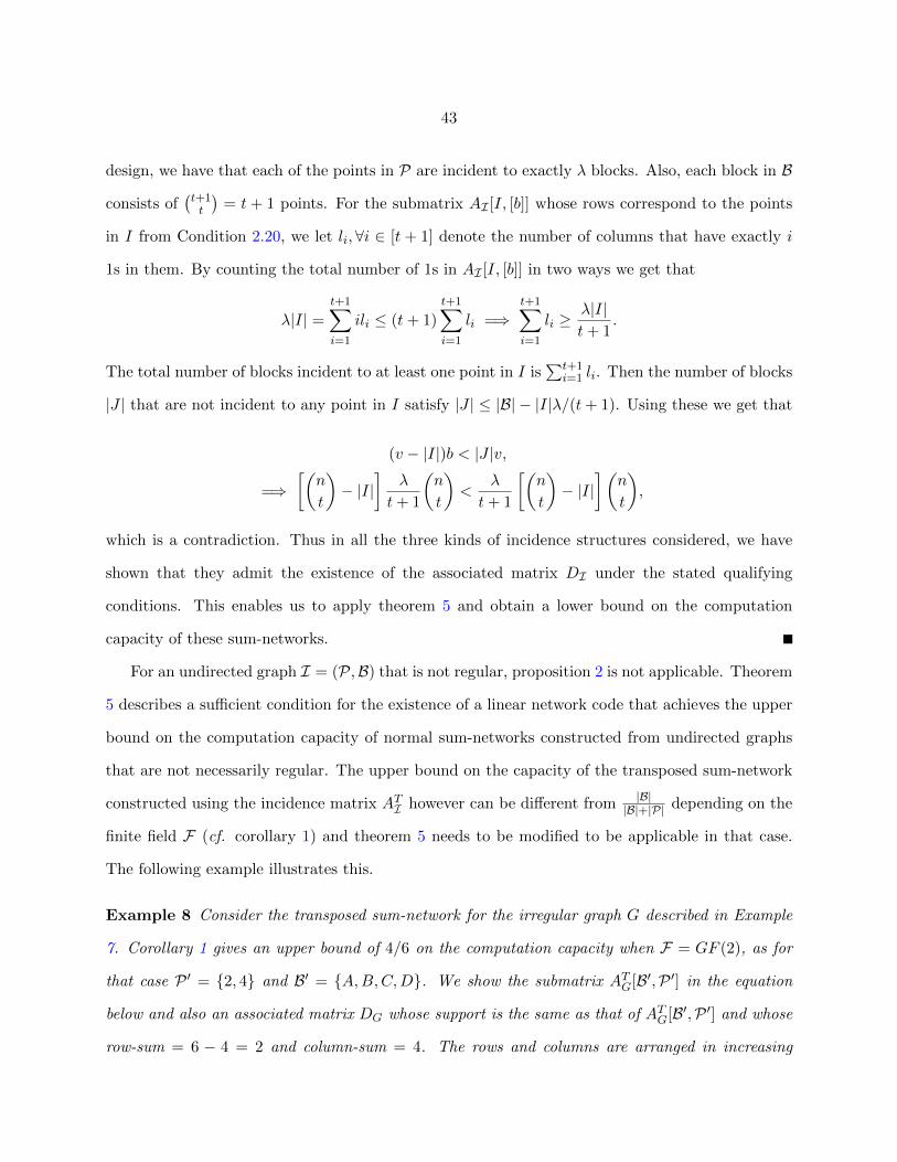
43

design, we have that each of the points in P are incident to exactly λ blocks. Also, each block in B

consists of(t+1t

)= t + 1 points. For the submatrix AI [I, [b]] whose rows correspond to the points

in I from Condition 2.20, we let li,∀i ∈ [t + 1] denote the number of columns that have exactly i

1s in them. By counting the total number of 1s in AI [I, [b]] in two ways we get that

λ|I| =t+1∑i=1

ili ≤ (t+ 1)t+1∑i=1

li =⇒t+1∑i=1

li ≥λ|I|t+ 1

.

The total number of blocks incident to at least one point in I is∑t+1

i=1 li. Then the number of blocks

|J | that are not incident to any point in I satisfy |J | ≤ |B| − |I|λ/(t+ 1). Using these we get that

(v − |I|)b < |J |v,

=⇒[(n

t

)− |I|

]λ

t+ 1

(n

t

)<

λ

t+ 1

[(n

t

)− |I|

](n

t

),

which is a contradiction. Thus in all the three kinds of incidence structures considered, we have

shown that they admit the existence of the associated matrix DI under the stated qualifying

conditions. This enables us to apply theorem 5 and obtain a lower bound on the computation

capacity of these sum-networks.

For an undirected graph I = (P,B) that is not regular, proposition 2 is not applicable. Theorem

5 describes a sufficient condition for the existence of a linear network code that achieves the upper

bound on the computation capacity of normal sum-networks constructed from undirected graphs

that are not necessarily regular. The upper bound on the capacity of the transposed sum-network

constructed using the incidence matrix ATI however can be different from |B||B|+|P| depending on the

finite field F (cf. corollary 1) and theorem 5 needs to be modified to be applicable in that case.

The following example illustrates this.

Example 8 Consider the transposed sum-network for the irregular graph G described in Example

7. Corollary 1 gives an upper bound of 4/6 on the computation capacity when F = GF (2), as for

that case P ′ = {2, 4} and B′ = {A,B,C,D}. We show the submatrix ATG[B′,P ′] in the equation

below and also an associated matrix DG whose support is the same as that of ATG[B′,P ′] and whose

row-sum = 6 − 4 = 2 and column-sum = 4. The rows and columns are arranged in increasing

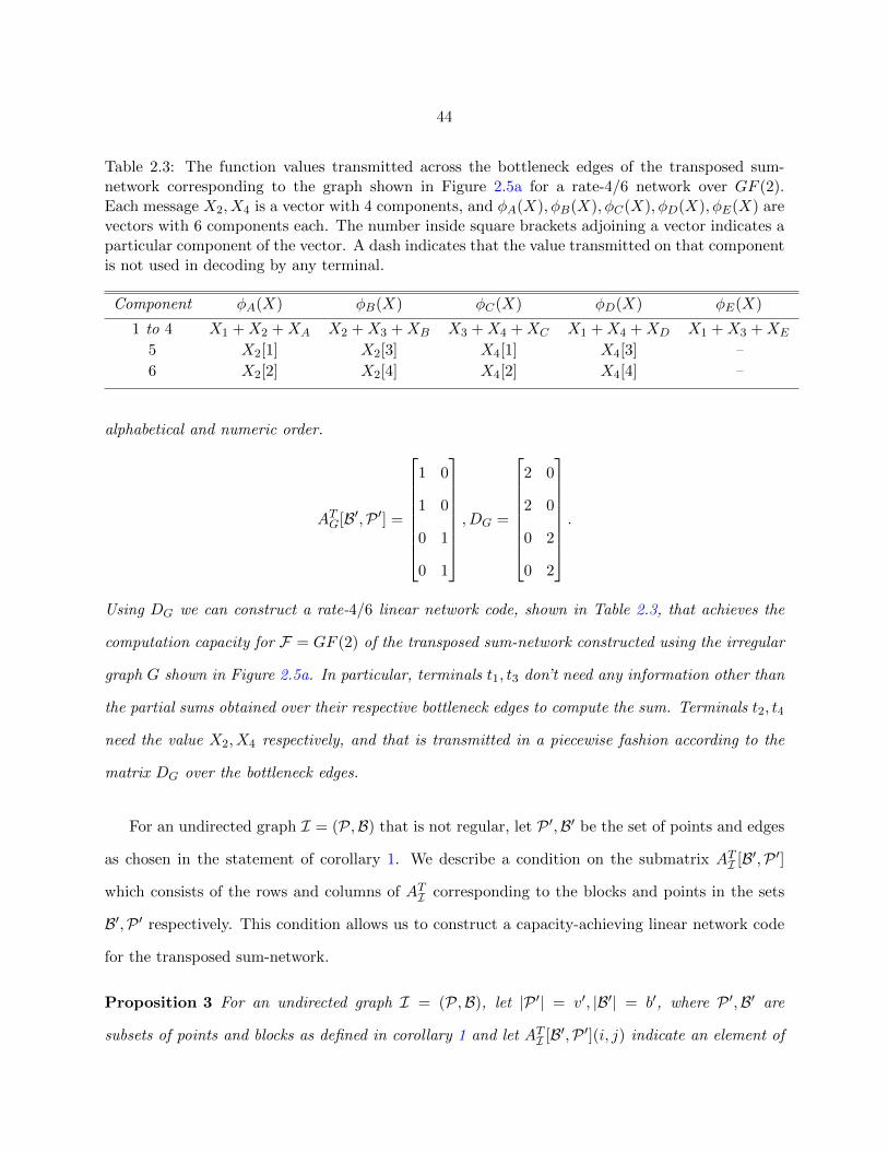
44

Table 2.3: The function values transmitted across the bottleneck edges of the transposed sum-network corresponding to the graph shown in Figure 2.5a for a rate-4/6 network over GF (2).Each message X2, X4 is a vector with 4 components, and φA(X), φB(X), φC(X), φD(X), φE(X) arevectors with 6 components each. The number inside square brackets adjoining a vector indicates aparticular component of the vector. A dash indicates that the value transmitted on that componentis not used in decoding by any terminal.

Component φA(X) φB(X) φC(X) φD(X) φE(X)

1 to 4 X1 +X2 +XA X2 +X3 +XB X3 +X4 +XC X1 +X4 +XD X1 +X3 +XE

5 X2[1] X2[3] X4[1] X4[3] –

6 X2[2] X2[4] X4[2] X4[4] –

alphabetical and numeric order.

ATG[B′,P ′] =

1 0

1 0

0 1

0 1

, DG =

2 0

2 0

0 2

0 2

.

Using DG we can construct a rate-4/6 linear network code, shown in Table 2.3, that achieves the

computation capacity for F = GF (2) of the transposed sum-network constructed using the irregular

graph G shown in Figure 2.5a. In particular, terminals t1, t3 don’t need any information other than

the partial sums obtained over their respective bottleneck edges to compute the sum. Terminals t2, t4

need the value X2, X4 respectively, and that is transmitted in a piecewise fashion according to the

matrix DG over the bottleneck edges.

For an undirected graph I = (P,B) that is not regular, let P ′,B′ be the set of points and edges

as chosen in the statement of corollary 1. We describe a condition on the submatrix ATI [B′,P ′]

which consists of the rows and columns of ATI corresponding to the blocks and points in the sets

B′,P ′ respectively. This condition allows us to construct a capacity-achieving linear network code

for the transposed sum-network.

Proposition 3 For an undirected graph I = (P,B), let |P ′| = v′, |B′| = b′, where P ′,B′ are

subsets of points and blocks as defined in corollary 1 and let ATI [B′,P ′](i, j) indicate an element of

45

the submatrix for indices i ∈ [b′], j ∈ [v′]. Suppose there is a matrix DI of dimension b′ × v′ such

that

DI(i, j) = 0, if ATI [B′,P ′](i, j) = 0,b′∑i=1

DI(i, j) = b′, for all j ∈ [v′], and

v′∑j=1

DI(i, j) = v′, for all i ∈ [b′].

Then there is linear network code of rate b′

b′+v′ that allows each terminal in the transposed sum-

network constructed using I to compute the required sum.

Proof: We describe a rate-b′/(b′ + v′) network code that enables each terminal to compute

the sum. Then by corollary 1 we know that this is a capacity-achieving code. Since this is a

transposed sum-network, the bottleneck edges in the sum-network correspond to the blocks in the

undirected graph I. The first b′ components transmitted over each bottleneck is obtained by the

following equation.

φi(X)[1 : b′] = XBi +∑

j:pj∈Bi

Xpj , for all Bi ∈ B.

We show that this partial sum satisfies all the terminals in the set {tBi : Bi ∈ B} ∪ {tpj : pj /∈ P ′}.

Terminals in {tBi : Bi ∈ B} can recover the sum as all messages not present in the partial sum are

available to tBi through direct edges. For terminals in the set {tp : p /∈ P ′}, they carry out the

following operation as a part of their decoding procedure.

∑i:Bi∈〈p〉

φi(X)[1 : b′] =∑

i:Bi∈〈p〉

XBi +∑

j:pj∈Bi

Xpj

(2.21)

=∑

i:Bi∈〈p〉

XBi +∑

j:{p,pj}∈B

ppTj Xpj + deg(p)Xp. (2.22)

For pj 6= p, we have that ppTj = 1 if {p, pj} ∈ B. Also by condition on the points that are not in

P ′, we have that deg(p) ≡ 1 (mod ch(F)), and hence all the coefficients in the above partial sum

are 1. The messages in the set {XB : B /∈ 〈p〉} ∪ {Xpj : {pj , p} /∈ B} are available to tp through

direct edges and hence it can recover the sum.

46

The remaining v′ components available on the bottleneck edges {ei : Bi ∈ B′} are used to

transmit information that enable the terminals in the set {tp : p ∈ P ′} to compute the sum.

Specifically, we construct a flow on a bipartite graph whose one part corresponds to the points

in P ′ and the other part corresponds to the blocks in B′, with incidence being determined by the

submatrix ATI [B′,P ′]. Since there exists a matrix DI with specified row and column sums, we can

use it to construct a flow on the bipartite graph such that the messages in the set {Xpi : pi ∈ P ′}

are transmitted in a piecewise fashion over the bottleneck edges {ej : Bj ∈ B′} in a manner similar

to the proof of theorem 5. Arguing in the same way, one can show that the network code based on

the flow solution allows each tp ∀p ∈ P ′ to obtain the value of Xp from the information transmitted

over the bottleneck edges in the set {ei : Bi ∈ 〈p〉}. Terminal tp computes the sum in eq. (2.21)

as a part of its decoding procedure. Since deg(p) 6≡ 1 (mod ch(F)), every term in the RHS of

eq. (2.22) except Xp has its coefficient as 1. But since tp knows the value of Xp it can subtract a

multiple of it and recover the relevant partial sum. The messages not present in this partial sum

are available to tp through direct edges and hence it can also compute the value of the sum.

Proposition 2 describes families of incidence structures for which the sum-networks constructed

admit capacity-achieving linear network codes. The upper bound on the computation capacity

of these sum-networks is obtained from Corollaries 1, 2 and 4. We now describe a rate-1 linear

network code for the sum-networks when their corresponding incidence structures do not satisfy

the qualifying conditions for the upper bounds. By theorem 1, the computation capacity of any

sum-network obtained using the SUM-NET-CONS algorithm is at most 1.

Proposition 4 For an incidence structure I = (P,B) and a finite field F , there exists a rate-1

linear network code that satisfies the following listed sum-networks. If

• I is a 2-(v, k, 1) design:

– the normal sum-network with ch(F) | k − 1,

– the transpose sum-network with ch(F) | v−kk−1 ,

• I is a t-(v, t+ 1, λ) design:

47

– the normal sum-network obtained using the higher incidence matrix with ch(F) | t,

– the transpose sum-network obtained using the higher incidence matrix with ch(F) | λ−1.

Proof: Suppose we construct a sum-network using the SUM-NET-CONS algorithm on a

(0, 1)-matrix A of dimension r × c. If ATA = (ATA)#, the following rate-1 linear network code

φi(X) = Xpi +∑

j:Bj∈〈pi〉

XBj , ∀ i ∈ [r],

satisfies every terminal in the sum-network in the following manner. A terminal tpi , ∀i ∈ [r] receives

all the messages not present in the partial sum transmitted along ei through direct edges, and hence

it can compute the sum. A terminal tB, ∀B ∈ B can carry out the following operation.

∑i:pi∈Bj

φi(X)=∑pi∈B

Xpi +∑pi∈B

∑Bj∈〈pi〉

XBj

=∑pi∈B

Xpi +∑

l:Bl∈〈Bj〉

BTl BjXBl .

Since ATA = (ATA)#, all the coefficients in the above sum are 1 and∑

i:pi∈Bj φi(X) is equal to

the sum of all the messages in the set {Xpi : pi ∈ Bj} ∪ {XB : B ∈ 〈Bj〉}. All the messages that

are not present in this set are available to tBj through direct edges.

Such a rate-1 linear network code gives us our proposition in the following manner. Let AI

be the v × v−1k−1 incidence matrix for a 2-(v, k, 1) design and let A′I be the higher incidence matrix

as defined in corollary 2 for a t-(v, t + 1, λ) design with λ 6= 1. Then, we have (from proofs of

Corollaries 2, 4)

ATIAI − (ATIAI)# = (k − 1)I,

AIATI − (AIA

TI )# =

v − kk − 1

I,

A′TI A

′I − (A

′TI A

′I)# = tI,

A′IA′TI − (A′IA

′TI )# = (λ− 1)I.

Thus, whenever any of the above matrices is a zero matrix, we have a scalar linear network code

that achieves the computation capacity of the associated sum-network.

48

2.7 Discussion and comparison with prior work

The discussion in Sections 2.5 and 2.6 establishes the computation capacity for sum-networks

derived from several classes of incidence structures. We now discuss the broader implications of

these results by appealing to existence results for these incidence structures. BIBDs have been the

subject of much investigation in the literature on combinatorial designs. In particular, the following

two theorems are well-known.

Theorem 6 [21, Theorem 6.17] There exists a (v, 3, 1)-BIBD (also known as a Steiner triple sys-

tem) if and only if v ≡ 1, 3 (mod 6); v ≥ 7.

Theorem 7 [21, Theorem 7.31] There exists a (v, 4, 1)-BIBD if and only if v ≡ 1, 4 (mod 12); v ≥

13.

In particular, these results show that there are an infinite family of Steiner triple systems and

BIBDs with block size 4 and λ = 1. Since k = 3 for any Steiner triple system, we can demonstrate

the existence of sum-networks whose computation capacity is greatly affected by the choice of the

finite field F used for communication.

Proposition 5 Consider the normal sum-network constructed using a 2-(v, 3, 1) design. If ch(F) =

2, then the computation capacity of the sum-network is 1. For odd ch(F), the computation capacity

is 65+v . For the normal sum-network constructed using a (v, 4, 1)-BIBD, the computation capacity

is 1 if ch(F) = 3 and 1211+v otherwise.

Proof: The number of blocks in a 2-(v, 3, 1) design is equal to v(v−1)/6. From corollary 2, if

ch(F) is odd, then the computation capacity of the sum-network constructed using a Steiner triple

system is at most vv+v(v−1)/6 = 6

5+v . Moreover by proposition 2, we can construct a linear network

code with rate equal to the upper bound. On the other hand, if ch(F) = 2, then the computation

capacity of the same sum-network is 1 by proposition 4.

The number of blocks in a 2-(v, 4, 1) design is v(v − 1)/12. We can recover the result for the

computation capacity of a normal sum-network constructed using it in a manner similar to the

previous case.

49

Thus, this result shows that for the same network, computing the sum over even characteristic

has capacity 1, while the capacity goes to zero as O(1/v) for odd characteristic. Moreover, this

dichotomy is not unique to the prime number 2. Similar results hold for sum-networks derived from

higher incidence structures (cf. corollary 4).

Theorem 8 [35] For two integers t, v such that v ≥ t + 1 > 0 and v ≡ t (mod (t + 1)!2t+1), a

t-(v, t+ 1, (t+ 1)!2t+1) design with no repeated blocks exists.

The number of blocks in a t-(v, t + 1, (t + 1)!2t+1) design can be evaluated to be(vt

) (t+1)!2t+1

t+1 . We

consider the normal sum-network obtained using the higher incidence matrix of this t-design. If

ch(F) - t, then by corollary 4 and proposition 2, we have that the computation capacity of this

sum-network is (vt

)(vt

)+(vt

) (t+1)!2t+1

t+1

=1

1 + t!2(t+ 1)!2t−1.

On the other hand, if ch(F) is a divisor of t, then by theorem 1 and proposition 4 we have that the

computation capacity of the normal sum-network constructed using the higher incidence matrix is

1. Thus for the same sum-network, computing the sum over a field whose characteristic divides

the parameter t can be done at rate = 1. However, if the field characteristic does not divide t,

zero-error computation of the sum can only be done at a rate which goes to zero as O((

te

)−t2).

Theorem 6 describes an infinite family of BIBDs with k = 3 and λ = 1. There are further

existence results for BIBDs with λ = 1 and k 6= 3. In particular, for λ = 1, k ≤ 9 there exist BIBDs

with value of v as given in Table 3.3 in [36, Section II.3.1]. As an example, if k = 5, then there

exists a 2-(v, 5, 1) design whenever v ≡ 1, 5 (mod 2)0. For any choice of a BIBD from this infinite

family, we can construct a corresponding normal sum-network, whose computation capacity for a

particular finite field can be found using corollary 2 and proposition 2. Even though theorem 4

states the existence of t-designs for v, t that satisfy the qualifying conditions, explicit constructions

of such t-designs with t ≥ 6 are very rare.

For a transposed sum-network obtained from an undirected graph that is not regular, the

computation capacity can show a more involved dependence on the finite field alphabet as the

following example demonstrates.

50

S6 S14 S10

a b c

Figure 2.6: The schematic shown represents an undirected graph with three components: S6, S14

and S10. St denotes the star graph on t + 1 vertices, with only one vertex having degree t whilethe rest have degree 1. The vertices with the maximum degree in the three star graphs are a, b, crespectively. In addition, a is connected to b and b is connected to c, such that deg(a) = 7,deg(b) =16, deg(c) = 11.

Example 9 Consider the transposed sum-network obtained by applying the SUM-NET-CONS al-

gorithm on the undirected graph I shown in Figure 2.6. Corollary 1 gives us an upper bound on

the computation capacity of the transposed sum-network based on the finite field alphabet F . The

upper bound for three different choices of F is as follows.

• F = GF (2): Then P ′ = {b}, so the upper bound is 16/(16 + 1) = 16/17.

• F = GF (3): Then P ′ = {c}, so the upper bound is 11/(11 + 1) = 11/12.

• F = GF (5): Then P ′ = {a}, so the upper bound is 7/(7 + 1) = 7/8.

We use proposition 3 to check if we can construct a linear network code in each case that has the

same rate as the respective upper bound. To do that, we focus on the appropriate submatrix of AI

for each case and see if it satisfies the required condition on row and column sums. The rows of

AI corresponding to the vertices a, b, c (in order) are shown below.16 1 0 · · · 0

06 1 114 1 010

0 · · · 0 1 110

,where 1,0 indicate all-one and all-zero row vectors of size specified by their subscripts. Using

this, one can verify that the appropriate submatrix for each of the three choices of F satisfies the

conditions of proposition 3 and hence we can construct a capacity-achieving linear network code in

each case.

51

Thus, as the previous example demonstrates, the computation capacity of a particular sum-

network need not take just one of two possible values, and can have a range of different values

based on the finite field chosen. We can generalize the example to obtain sum-networks that have

arbitrary different possible values for their computation capacity.

Our constructed sum-networks have a unit maximum flow between any source and any termi-

nal. We can modify our construction so that each edge in the network has a capacity of α > 1.

Specifically, the following result can be shown.

Proposition 6 Let N denote the sum-network obtained by applying the SUM-NET-CONS algo-

rithm on a matrix A of dimension r × c. For an integer α > 1, let Nα denote the sum-network

obtained by modifying the SUM-NET-CONS algorithm such that Nα has the same structure as N

but each edge eα in Nα has cap(eα) = α > 1. Then, if A satisfies the qualifying conditions in

Theorems 2 and 5, the computation capacity of Nα is αrr+c .

Proof: Since A satisfies the conditions in theorem 5, there exists a (m,n) vector linear

network code with m = r, n = r + c. For every unit-capacity edge in N , we have α unit-capacity

edges between the same tail and head in Nα. At the tail of every edge in Nα, we can apply the

same network code except now we have α distinct edges on which we can transmit the encoded

value. Thus we need transmit only r+cα symbols on each of those edges. If r+c

α is not an integer,

one can appropriately multiply both m,n with a constant. This modified network code has rate

= αrr+c . Since A also satisfies the conditions in theorem 2, we have that an upper bound on the

computation capacity of N is r/(r+ c). Applying the same argument on Nα, we get that an upper

bound on the computation capacity of Nα is αrr+c . This matches the rate of the modified vector

linear network code described above.

This result can be interpreted as follows. Consider the class of sum-networks where the maxi-

mum flow between any source-terminal pair is at least α. Our results indicate, that for any α, we

can always demonstrate the existence of a sum-network, where the computation capacity is strictly

smaller than 1. Once again, this indicates the crucial role of the network topology in function

computation.

52

2.7.1 Comparison with prior work

The work of Rai and Das [29] is closest in spirit to our work. In [29], the authors gave a

construction procedure to obtain a sum-network with computation capacity equal to p/q, where

p, q are any two co-prime natural numbers. The procedure involved first constructing a sum-

network whose capacity was 1/q. Each edge in this sum-network had unit-capacity. By inflating

the capacity of each edge in the sum-network to p > 1, the modified sum-network was shown to

have computation capacity as p/q.

Our work is a significant generalization of their work. In particular, their sum-network with

capacity 1/q can be obtained by applying the SUM-NET-CONS algorithm to the incidence matrix

of a complete graph on 2q − 1 vertices [30]. We provide a systematic procedure for constructing

these sum-networks for much larger classes of incidence structures.

In [29], the authors also posed the question if smaller sum-networks (with lesser sources and

terminals) with capacity as p/q existed. Using the procedure described in this paper, we can answer

that question in the affirmative.

Example 10 The normal sum-network for the undirected graph in Figure 2.5a has computation

capacity = 4/9 and has nine sources and terminals. To obtain a sum-network with the same

computation capacity using the method described in [29] would involve constructing the normal

sum-network for a complete graph on 17 vertices, and such a sum-network would have 153 source

nodes and terminal nodes each.

In [20], it was shown by a counter-example that for the class of sum-networks with |S| = |T | = 3,

a maximum flow of 1 between each source-terminal pair was not enough to guarantee solvability

(i.e., no network code of rate 1 exists for the counterexample). It can be observed that their counter-

example is the sum-network shown in Figure 2.2a. Our characterization of computation capacity

for a family of sum-networks provides significantly more general impossibility results in a similar

vein. In particular, note that for the α-capacity edge version of a sum-network, the maximum flow

between any source-terminal pair is at least α. Then suppose we consider the class of sum-networks

53

with |S| = |T | = x = β(β + 1)/2 for some β ∈ N. Consider a complete graph Kβ = (V,E) on β

vertices; then |V |+ |E| = x. Consider the sum-network obtained by applying the procedure on Kβ,

with each edge added having capacity as α. Then the computation capacity of this sum-network

is αβ/x, which is less than 1 if α < (β + 1)/2. This implies that a max-flow of (β + 1)/2 between

each source-terminal pair is a necessary condition for ensuring all sum-networks with |S| = |T | = x

are solvable. When x cannot be written as β(β+ 1)/2 for some β, a similar argument can be made

by finding an undirected graph G = (V,E) (whose incidence matrix AG satisfies the condition in

theorem 5) such that |V | is minimal and |V |+ |E| = x.

2.8 Conclusions and future work

Sum-networks are a large class of function computation problems over directed acyclic net-

works. The notion of computation capacity is central in function computation problems, and

various counterexamples and problem instances have been used by different authors to obtain a

better understanding of solvability and computation capacity of general networks. We provide

an algorithm to systematically construct sum-network instances using combinatorial objects called

incidence structures. We propose novel upper bounds on their computation capacity, and in most

cases, give matching achievable schemes that leverage results on the existence of non-negative in-

teger matrices with prescribed row and column sums. We demonstrate that the dependence of

computation capacity on the underlying field characteristic can be rather strong.

There are several opportunities for future work. Our proposed linear network codes for the con-

structed sum-networks require the correspondence incidence structures to have a specific property.

In particular, our techniques only work in the case when ATA − (ATA)# is a diagonal matrix. It

would be interesting to find capacity achieving network codes in cases when ATA− (ATA)# is not

diagonal. More generally, it would be interesting to obtain achievability schemes and upper bounds

for sum-networks with more general topologies.

54

CHAPTER 3. FUNCTION COMPUTATION ON A DIRECTED ACYCLIC

NETWORK

1 We study the rate region of variable-length source-network codes that are used to compute

a function of messages observed over a network. The particular network considered here is the

simplest instance of a directed acyclic graph (DAG) that is not a tree. Existing work on zero-error

function computation in DAG networks provides bounds on the computation capacity, which is a

measure of the amount of communication required per edge in the worst case. This work focuses on

the average case: an achievable rate tuple describes the expected amount of communication required

on each edge, where the expectation is over the probability measure of the source messages. We

describe a procedure to obtain outer bounds to the rate region for computing an arbitrary demand

function at the terminal. A key fact used to specify these outer bounds is the Schur-concave

property of the entropy function. We evaluate these bounds for certain example demand functions.

When the demand function is the finite field sum of messages from GF (2), we show a network code

that achieves the outer bound. When the demand function is the sum of three bit messages over

the real numbers, there is a gap in the sum-rate between the outer bound and the network code

that we use.

3.1 Introduction

Computing functions of data observed over a network is a well-motivated problem, and different

frameworks addressing the problem have been studied in the literature. Broadly speaking, a general

function computation problem can be modeled in the following manner. A directed acyclic graph

(DAG) is used to model a communication network. Its vertices denote nodes of the network that are

assumed to have unrestricted computational power and storage capacity. The edges denote one-way

1A part of this work was presented at the 2016 IEEE International Symposium on Information Theory.

55

communication links that can be thought of as noiseless bit-pipes. Each node can act as a decoder

on the information received on its incoming edges and as an encoder for information transmitted

on its outgoing edges. Some of the nodes in the network, called the source nodes, observe discrete-

valued source messages that take values in a finite alphabet. The random process generating the

source messages is assumed to be stationary and memoryless. There is a single terminal node

that wishes to compute losslessly a discrete-valued function of all the source messages using the

information it receives on its incoming edges. A solution to such a function computation problem

will specify the communication carried out on each link and the information processing done at

each node of the network. We are interested in finding the minimal communication required for

solving a given problem instance. The amount of communication in a network can be specified by

a rate tuple that has as many entries as the number of edges in the network. Each entry denotes

the rate of the code employed on the corresponding edge in the network. As remarked in [37], this

problem in its full generality encompasses several different areas in information theory, and as such,

existing literature focuses on simplified versions that highlight different aspects of the problem.

If there is just one encoder and one decoder connected by a noiseless communication link, and

the decoder wants to compute the identity function for the message, then it is a standard source

coding problem2. When there is some coded side information available through an additional link

at the decoder, then the optimal rate pair is given by the Ahlswede–Korner–Wyner solution [38,

Thm. 10.2]. Extending this one-help-one solution to a two-help-one scenario is not optimal, as was

demonstrated for a particular two-help-one problem instance by Korner and Marton [1].

Consider now the case of two encoders, connected by two separate links to a decoder which is

interested in computing the identity function on the pair of source messages. The optimal rate pair

for this distributed source coding problem is known to be the Slepian–Wolf rate region, and this

solution can be extended to multiple encoders each of which are directly connected to the decoder

via a separate link [38, Chap. 10].

2If the demand function is not identity, then it is a source coding problem for the random function value, as thefunction can be precomputed in the encoding process.

56

In reproducing the source messages at the terminal in the above scenarios, the coding schemes

allow for an ε-block error that can be made as small as desired by choosing asymptotically large

block lengths. Concurrently, work on zero-error source coding with side information was initiated

by Witsenhausen [39]. With X being the source message and Y the side information, he defined a

confusability graph GX for X that tells us which realizations of X must be given distinct codewords

by the encoder in order to attain zero-error. The optimum number of distinct codewords required

was shown to be the graph chromatic number χ(GX); for encoding multiple (say, k) instances it is

χ(GkX) where GkX denotes the k-wise AND product graph of GX . Thus when χ(GkX) < (χ(GX))k,

block encoding multiple instances allows one to reduce the number of distinct codewords required.

The above idea along with the probability information of X was used to find the expected number

of bits that must be transmitted by the encoder in [40]. For the case when the codewords are

restricted to be prefix-free, their expected length was shown in [40] to be within one bit of the

chromatic entropy Hχ(GX , X) of the probabilistic graph (GX , X). When multiple instances are

block encoded, the asymptotic per-instance expected codeword length is limk→∞1kHχ(G∨kX , Xk),

where G∨kX is the k-wise OR product graph of GX . This limit was shown to be the graph entropy of

(GX , X) in [40]. More information about the possible savings due to encoding multiple instances

can be found in [41, Sec. XI].

In a function computing problem, the terminal would want to compute a general demand

function of the messages and not necessarily the identity function. The work done in [2] considered

computing a function on the setup of the source coding with side information problem, and allowed a

vanishing block-error probability. They defined the conditional graph entropy H(GX , X|Y ) for the

probabilistic graph (GX , X|Y ) of X given Y and showed that it is equal to the optimal number of

bits per-instance of X that must be communicated by the encoder when asymptotically large block

lengths are used. This was extended by the authors in [3] where they defined a conditional chromatic

entropy of a probabilistic graph and showed that limk→∞1kHχ(G∨kX , Xk|Y k) = H(GX , X|Y ). This

gave a graph coloring procedure to obtain codes with rate close to the lower bound of [2].

57

Function computation was also approached in the distributed setting, where two encoders sep-

arately encode X and Y such that the decoder is able to compute F (X,Y ) losslessly. This scenario

is closer to the source coding with side information problem than the distributed source coding

problem because of the following. Any demand function can be computed at the decoder after com-

municating each of the source messages to it, thus the Slepian–Wolf region is an inner bound to the

rate region of a function computation problem on the same network. Korner and Marton showed in

[1] that if the decoder wants to decode just Z, then the rate tuple (RX , RY , RZ) = (H(Z), H(Z), 0)

is achievable for the case when Z = X ⊕ Y , X and Y are a doubly symmetric binary source

pair and ⊕ denotes modulo-2 sum. This rate tuple, with RZ = 0, can be interpreted as the de-

coder wanting to compute the modulo-2 sum using the information obtained from the X and Y

encoders. This view was taken by Han and Kobayashi in [42] where, subject to the constraint

Pr(x, y) > 0, ∀(x, y) ∈ X ×Y, they gave necessary and sufficient conditions on the demand function

F (X,Y ) for which the Slepian–Wolf region for the source pair (X,Y ) coincides with the rate region

of the function computation problem. This gave a dichotomy in the class of bivariate functions

that only depended on the X × Y function realization table and not on Pr(X,Y ), except through

the positivity constraint.

The authors in [3] also considered distributed function computation, where they showed that

if Pr(X,Y ) satisfied a restrictive ‘zigzag’ condition, then coloring the confusability graphs G∨kX

and G∨kY and then using Slepian–Wolf code is optimal for asymptotic block length. This sufficient

condition was relaxed in [43] to a coloring connectivity condition by taking into account the function

value. This condition was shown to characterize the rate region for function computation on one-

stage tree-networks. It also gave an inner bound to the rate region of a general tree network. The

rate region for a multi-stage tree-network when every source message at a vertex in the network

satisfies a local Markovian property was characterized in [44]. The function computation scenarios

described above all allowed for a vanishing block-error probability with asymptotically large block

lengths.

58

In this paper, we study the problem of zero-error function computation over a simple DAG

network that is not a tree, shown in Fig. 3.1. We assume that the three source messages are

independent and the terminal wants to compute an arbitrary specified demand function of the

messages. We allow for block encoding and decoding of multiple instances at the sources and the

terminal. Even with the independence assumption, characterizing the rate region of this function

computation problem is difficult as was observed in [49], where the problem of computing a par-

ticular arithmetic sum demand function on the same DAG network was considered. We describe

works closely related to our problem next.

3.1.1 Related work

Zero-error function computation over a graphical network using network coding [4], [5] was

studied in [45]. There they considered two variants of the communication load on the network,

called worst-case and average-case complexity, depending on whether the probability information

of the source messages was used or not. They characterized the rate region of achievable rate

tuples that allowed zero-error function computation in tree-networks, each entry in a rate tuple

was the rate of a code employed on the corresponding edge in the tree-network. They also made

the observation that finding the rate region of a DAG network is significantly challenging because of

multiple paths between a source node and the terminal, which allows for different ways of combining

information at the intermediate nodes.

Zero-error function computation was also studied in [15], where the authors defined the com-

putation capacity, which is a single number, of a function computation problem instance. This is a

generalization of the coding capacity of a network (c.f. [8, Sec. VI], [9]), which is the supremum of

the ratio kn over all achievable (k, n) fractional coding solutions for that communication network. A

(k, n) fractional network code is one in which k source messages are block encoded at each encoder

and every edge in the network transmits n symbols from the alphabet in one channel use. The

authors in [15] characterized the computation capacity of multi-stage tree-networks by finding the

necessary and sufficient amount of information that must be transmitted across all graph cuts that

59

separate one or more source nodes from the terminal. Upper bounds on the computation capacity

of DAG networks are more complicated and have been obtained in [16], [47]. These upper bounds

were shown to be unachievable for a function computation problem on a particular DAG in recent

work [52, Sec. V]. An illuminating example in the search for improved upper bounds for function

computation on DAG networks has been the problem of computing the arithmetic sum of three

source bits over the network shown in Fig. 3.1. By counting the necessary and sufficient number of

codewords required, the computation capacity for this problem was evaluated to be log6 4 in [15,

Sec. V].

While the upper bounds for DAG networks described above hold for the worst-case scenario,

it can be seen in the arithmetic sum example that we can do better in the average-case scenario

by using the probability information of the source messages. For instance, suppose that the three

source bits observed at s1, s2 and s3 are equally likely to be 0 or 1, i.e., they are independent

Bernoulli(1/2) random variables. By letting the number of symbols transmitted across the edges

be a random variable N (instead of a fixed n for every k source bits as in the (k, n) fractional network

code framework3), it can be seen that the computation rate kEN = 0.8 > log6 4 is achievable (c.f.

Eg. 11). The work in [49] also gave an upper bound of 8/9 for the computation capacity of this

arithmetic sum example in the framework of variable-length network codes.

It can be seen that an upper bound to the computation capacity corresponds to an outer bound

to the rate region of a function computation problem. We use the framework of a source-network

code as used for zero-error network coding in [50]. Correspondingly, the quantity of interest here

is the zero-error function computation rate region, and we provide outer bounds to this rate region

for computing an arbitrary specified demand function on the network shown in Fig. 3.1. We

summarize our contributions below.

3As described in [49], for finding the computation capacity, it can be assumed w.l.o.g. that the message vectorXk

3 is available to both the encoders at s1 and s2. Then the random variable N is defined as a stopping time w.r.t.the pair of random variables transmitted over the edges (s1, t) and (s2, t).

60

3.1.2 Main contributions

• We compute lower bounds on the rates that must be used on the edges of the DAG in Fig.

3.1 in order to compute with zero-error an arbitrary demand function of the messages at the

terminal. This provides us an outer bound to the achievable rate region.

• The technique used for obtaining the lower bounds involved lower bounding the conditional

entropy of the descriptions transmitted on the edges given the demand function value. This

was done by first finding a family of probability mass functions (p.m.f.) that must necessarily

contain the conditional p.m.f. of the descriptions transmitted by any valid source-network

code for the problem. The required lower bound was then obtained by finding the entropy-

minimizing p.m.f. in this family. This p.m.f. was found using the Schur-concave property of

the entropy function.

• Computing the arithmetic sum of three bits over the DAG in Fig. 3.1 was considered in

[49]. For that case, our procedure here gives a tighter lower bound for the sum-rate. We also

demonstrate that our outer bound for the rate region is tight when the demand function is

set to be the sum of three bits over GF (2).

The paper is organized as follows. Section 3.2 describes the problem setup formally and motivates

the use of variable-length network codes as defined in Section 3.2.1. Section 3.3 describes the

procedure used to obtain outer bounds to the rate region for computing an arbitrary demand

function over the network in Figure 3.1. Central to our approach are lower bounds to the conditional

entropy of the descriptions transmitted, and these are described and illustrated using a running

example in Section 3.3.1. We also consider two other example demand functions in Sections 3.3.3

and 3.3.4. Section 3.4 concludes the chapter and lists some avenues for future work.

3.2 Problem formulation

The edges in Figure 3.1 (later denoted by an ordered pair of vertices) have unit-capacity. We use

the notation of a standard network code from [15]. In what follows, all logarithms denoted as log are

61

s3

s1 s2

t

Figure 3.1: A directed acyclic network with three sources, two of which also act as relay nodes, andone terminal.

to the base 2 unless specified otherwise. Suppose that Z is the alphabet used for communication,

and |Z| > 1. Vertices s1, s2, s3 are the three source nodes that observe source messages X1, X2, X3

respectively, each from a discrete alphabet A with size |A| > 1. The sources are assumed to be

i.i.d. uniformly distributed over A. Terminal node t wants to compute with zero error and zero

distortion a known demand function:

f : A×A×A → B

f(X1, X2, X3) 7→ B

where B is a discrete alphabet of size |B| > 1. To avoid trivialities we assume that the demand

function is not constant in any of its three arguments. A (k, n) network code that satisfies the

terminal has the following components.

• An encoding function h(e)(·) associated with every edge e in the network:

h(s3,s1)(Xk3 ) : Ak → Zn

h(s3,s2)(Xk3 ) : Ak → Zn

h(s1,t)(Xk

1 , h(s3,s1)(Xk

3 ))

: Ak ×Zn → Zn

h(s2,t)(Xk

2 , h(s3,s2)(Xk

3 ))

: Ak ×Zn → Zn

Here the notation Xkj , j ∈ {1, 2, 3} denotes a block of k i.i.d. uniform messages.

• A decoding function ψ(·) used by the terminal t:

ψ(h(s1,t)(Xk

1 , h(s3,s1)(Xk

3 )), h(s2,t)(Xk2 , h

(s3,s2)(Xk3 )))

: Zn ×Zn → Bk

62

With slight abuse of notation we let f(Xk1 , X

k2 , X

k3 ) ∈ Bk denote the k values returned

by the demand function f(X1, X2, X3) when applied component-wise on a block of k i.i.d.

(X1, X2, X3) triples. That is,

f(Xk1 , X

k2 , X

k3 ) =

(f(X

(1)1 , X

(1)2 , X

(1)3 ), f(X

(2)1 , X

(2)2 , X

(2)3 ), . . . , f(X

(k)1 , X

(k)2 , X

(k)3 )),

where X(i)j denotes the ith component of Xk

j . By the zero-error criterion we have that

Pr{ψ(h(s1,t)(Xk

1 , Xk3 ), h(s2,t)(Xk

2 , Xk3 ))6= f(Xk

1 , Xk2 , X

k3 )}

= 0,

where the sample space consists of all realizations of the i.i.d. messages Xkj , j ∈ {1, 2, 3}.

If such a set of encoding and decoding functions exist for a choice of positive integers k and

n, we say that the network code computes the demand function and has computation rate =

k log |A|/(n log |Z|). The computation capacity for a particular demand function is defined to be

the supremum of all achievable computation rates.

The above framework is restrictive in the sense that the block length of the network code used

(i.e., the value of n) is the same for each edge in the network. If we know the probability distribution

associated with the message random variables and allow the block length of the network code on

edge e be a random variable Ne, then we can compress the descriptions transmitted on the edges

and obtain savings in the expected length E[Ne].

Example 11 Consider the problem of computing the sum over the real numbers (arithmetic sum)

of three bits, i.e. f(X1, X2, X3) = X1 + X2 + X3, on the network shown in Figure 3.1. The

messages X1, X2, X3 ∈ {0, 1}k and f(X1, X2, X3) ∈ {0, 1, 2, 3}k. This example was first considered

in [15], where they gave an optimal network code having computation rate log6 4 ≈ 0.77 to solve

it. The optimal network code transmits the value of X3 on the edges (s3, s1), (s3, s2) and the values

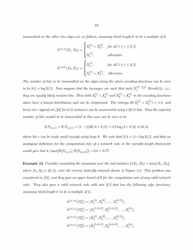
63

transmitted on the other two edges are as follows, assuming block length k to be a multiple of 2.

h(s1,t)(X1, X3) =

X

(i)1 +X

(i)3 , for all 1 ≤ i ≤ k/2

X(i)1 , otherwise.

h(s2,t)(X2, X3) =

X

(i)2 , for all 1 ≤ i ≤ k/2

X(i)2 +X

(i)3 , otherwise.

The number of bits to be transmitted on the edges using the above encoding functions can be seen

to be k(1 + log 3)/2. Now suppose that the messages are such that each X(i)j

i.i.d.∼ Bern(0.5), i.e.,

they are equally likely random bits. Then both X(i)1 +X

(i)3 and X

(i)2 +X

(i)3 in the encoding functions

above have a biased distribution and can be compressed. The entropy H(X(i)1 + X

(i)3 ) = 1.5, and

hence its ε-typical set [46] for k/2 instances can be enumerated using 1.5k/2 bits. Thus the expected

number of bits needed to be transmitted in this case can be seen to be

EN(s1,t) = EN(s2,t) = (1− ε)(3k/4 + k/2) + ε(k log2 3 + k/2) ≈ 5k/4,

where the ε can be made small enough using large k. We note that 5/4 < (1 + log 3)/2, and that an

analogous definition for the computation rate of a network code in the variable-length framework

would give that k/max{E[N(s1,t)],E[N(s2,t)]} = 0.8 > 0.77.

Example 12 Consider computing the maximum over the real numbers f(X1, X2) = max{X1, X2},

where X1, X2 ∈ {0, 1}, over the reverse butterfly network shown in Figure 3.2. This problem was

considered in [52], and they gave an upper bound of 2 for the computation rate of any valid network

code. They also gave a valid network code with rate 3/2 that has the following edge functions,

assuming block length k to be a multiple of 3.

h(s1,r3)(Xk1 ) = (X

(1)1 , X

(2)1 , . . . , X

(k/3)1 ),

h(s1,r1)(Xk1 ) = (X

(1+k/3)1 , X

(2+k/3)1 , . . . , X

(k)1 ),

h(s2,r4)(Xk2 ) = (X

(1)2 , X

(2)2 , . . . , X

(k/3)2 ),

h(s2,r1)(Xk2 ) = (X

(1+k/3)2 , X

(2+k/3)2 , . . . , X

(k)1 ),

64

s1 s2

r1

r3 r4

t

r2

Figure 3.2: A directed acyclic network with two sources, four relay nodes and one terminal.

h(r1,r2)(h(s1,r1)(Xk1 ), h(s2,r1)(Xk

2 )) = (max{X(1+k/3)1 , X

(1+k/3)2 }, . . . ,max{X(k)

1 , X(k)2 }),

h(r2,r3)(h(r1,r2)(h(s1,r1)(Xk1 ), h(s2,r1)(Xk

2 ))) = (max{X(1+k/3)1 , X

(1+k/3)2 }, . . . ,max{X(2k/3)

1 , X(2k/3)2 }),

h(r2,r4)(h(r1,r2)(h(s1,r1)(Xk1 ), h(s2,r1)(Xk

2 ))) = (max{X(1+2k/3)1 , X

(1+2k/3)2 }, . . . ,max{X(k)

1 , X(k)2 }),

h(r3,t)(h(s1,r3)(·), h(r2,r3)(·)) = (h(s1,r3)(·), h(r2,r3)(·)),

h(r4,t)(h(s2,r4)(·), h(r2,r4)(·)) = (h(s2,r4)(·), h(r2,r4)(·)),

where the last two equations state that the edges (r3, t), (r4, t) concatenate their inputs and forward

it, and we have omitted the arguments of certain edge functions (represented by a dot) for brevity.

Now consider the case when each X(i)j

i.i.d.∼ Bern(0.75), i.e., it takes the value 1 with probability

0.75 and 0 with probability 0.25. Since max{X(i)1 , X

(i)2 } has a biased p.m.f., we are able to compress

the descriptions transmitted on the edges. We describe a variable-length network code that has a

similar structure, except that the partitioning of the k components of X1 along the edges (s1, r3)

and (s1, r1) is different from the 1:2 ratio used before, and it uses typical set encoding. For the ith

component, the entropy values H(X(i)j ) ≈ 0.8113 and H(max{X(i)

1 , X(i)2 }) ≈ 0.3373 can be verified.

Set the value c , 1/(2−0.3373/(2 ·0.8113)) ≈ 0.558. Then the description transmitted on the edges

65

(s1, r3) and (s1, r1) are as follows.

h(s1,r3)(X1) = Tε[(X(1)1 , X

(2)1 , . . . , X

(k−ck)1 )]

h(s1,r1)(X1) = Tε[(X(1+k−ck)1 , X

(2+ck)1 , . . . , X

(k)1 )],

where Tε[·] indicates typical set encoding and a similar description of X2 is transmitted on the edges

(s2, r1) and (s2, r4). This partitioning is chosen so as to have the best possible rate within a class

of network codes that have the same structure as the initial network code described, as the following

computations indicate.

EN(s1,r1) = EN(s2,r1) = 0.8113 · ck = 0.4527k, EN(s1,r3) = EN(s2,r4) = 0.8113 · (1− c)k = 0.3586k,

EN(r1,r2) = 0.3373 · ck = 0.1882k, EN(r2,r3) = EN(r2,r4) = 0.1882k/2 = 0.0941k,

EN(r3,t) = EN(r4,t) = 0.0941k + 0.3586k = 0.4527k.

Thus we have that k/(maxall edges e E[Ne]) = k/(0.4527k) = 2.209 > 2.

The above examples illustrate the reduction in communication load that can be achieved by using

the knowledge of the probability distribution of the messages. The objective in this paper is to find

bounds on rates of variable-length network codes that are valid for a given function computation

problem. We first define the framework of variable-length network codes as adapted to the network

in Figure 3.1 next.

3.2.1 Variable-length network code for network in figure 3.1

We use the Source-Network Code framework as described in [50] and adapt it to the function

computation setting described above. The quantity of interest here is the rate region R, which is a

bounded region containing all achievable rate tuples R. Each rate tuple has four components, one

for each edge in the network. We define the source-network code and the admissible rate tuples

below.

Definition 7 Let Z∗ denote the set of all finite-length sequences with alphabet Z. A source-network

code Cf,k for computing f(Xk1 , X

k2 , X

k3 ) in the network of Figure 3.1 has the following components:

66

1. Encoding functions for edges e ∈ {(s3, s1), (s3, s2), (s1, t), (s2, t)}:

φ(s3,s1)(Xk3 ) : Ak → Z∗

φ(s3,s2)(Xk3 ) : Ak → Z∗

φ(s1,t)

(Xk

1 , φ(s3,s1)(Xk3 ))

: Ak ×Z∗ → Z∗

φ(s2,t)

(Xk

2 , φ(s3,s2)(Xk3 ))

: Ak ×Z∗ → Z∗

For brevity, we denote φ(s1,t)

(Xk

1 , φ(s3,s1)(Xk

3 ))

by the random variable Z1, and similarly

define the r.v.s Z2,Z31,Z32.

2. Decoding function for terminal t: ψt : Z∗ ×Z∗ → Bk is such that

Pr{ψt(Z1,Z2) 6= f(Xk1 , X

k2 , X

k3 )} = 0.

Thus the outputs of the encoders are variable length, and the terminal is equipped with a decoder

that takes in a pair of variable length inputs and returns without any error the block of k function

computations on the message tuple. The rate of a source-network code is defined below, taking

into account the different alphabets in which the messages and the codewords reside.

Definition 8 R = (R31, R32, R1, R2) is an admissible rate pair for the code Cf,k if for any ε > 0

there exists a sufficiently large k such that

log |Z|E `(Z1) ≤ k log |A|(R1 + ε)

where E `(Z1) is the expected length (in symbols from Z, and over the probability space of all message

realizations) of the codeword Z1. A similar definition is used for the rates R31, R32 and R2.

3.3 Bounds on the rate region for network in figure 3.1

We use a lower bound, reproduced from [51], on the expected length of the codewords trans-

mitted on the edges in terms of their entropy.

67

Lemma 3 (Adapted from Theorem 3 in [51]) The expected length of the best non-singular

code C?NS(Z) for a r.v. Z satisfies the following lower bound:

E ` (C?NS(Z)) ≥ H|Z|(Z)− 2 log|Z|(H|Z|(Z) + |Z|

).

Proof: Theorem 3 in [51] gives a lower bound for the expected length of a non-singular code

over binary alphabet in terms of the entropy of the source. We adapt their proof procedure for

codes over non-binary alphabet Z.

Let l1 ≤ l2 ≤ · · · ≤ lmax be the lengths over Z of the best non-singular code for Z. We

demonstrate a function g such that the set of lengths {g(li) : i = 1, 2, . . .} satisfy Kraft’s inequality,

i.e.,∑∞

i=1 |Z|−g(li) ≤ 1. Choose g(li) , li + 2blog|Z|(li + |Z| − 1)c. Since there are |Z|li different

non-singular codewords with length li and if lmax > li then all of them must have been used in the

best non-singular code, we have that

∑i

|Z|−li−2blog|Z|(li+|Z|−1)c =

lmax∑l1

|Z|li |Z|−li−2blog|Z|(li+|Z|−1)c ≤∞∑l=1

|Z|−(2blog|Z|(l+|Z|−1)c)

=

|Z|2−|Z|∑l=1

1

|Z|2 +

|Z|3−|Z|∑l=|Z|2−|Z|+1

1

|Z|4 +

|Z|4−|Z|∑l=|Z|3−|Z|+1

1

|Z|6 + · · ·

=|Z| − 1

|Z| +|Z| − 1

|Z|2 +|Z| − 1

|Z|3 + · · · = 1.

The above is also true if lmax → ∞. Thus there exists an uniquely decodable code for Z whose

codeword lengths are {dg(li)e : i = 1, 2, . . .}. Using random variable ` to denote the lengths of the

codewords in the best non-singular code for Z, we have that

H|Z|(Z) ≤ E(`+ 2blog|Z|(`+ |Z| − 1)c) ≤ E `+ 2E log|Z|(`+ |Z| − 1)(i)

≤ E `+ 2 log|Z|(E `+ |Z| − 1)

≤ E `+ 2 log|Z|(1 +H|Z| + |Z| − 1) =⇒ E ` ≥ H|Z|(Z)− 2 log|Z|(|Z|+H|Z|(Z)),

where inequality (i) above is true due to Jensen’s inequality.

Since the identity mapping is also a non-singular code for Z, we have that

E `(Z) =∑z

Pr{Z = z}`(z) ≥ E ` (C?NS(Z)) . (3.1)

68

Because of the zero-error requirement for the decoding function at the terminal, we can give a value

for what the sum rate R31 +R32 must be greater than.

Lemma 4 Consider an equivalence relation on Ak for which x3 ≡ x′3 if and only if for all

(x1,x2) ∈ Ak × Ak, we have that f(x1,x2,x3) = f(x1,x2,x′3). Define the function g(Xk

3 ) which

returns the equivalence class that Xk3 belongs to under the above relation. Then the range of g(Xk

3 )

is a subset of {1, 2, . . . , |A|k} and we have that R31 +R32 ≥ H(g(Xk3 ))/k log |A|.

Proof: Suppose that H|Z|(g(Xk3 )|Z31,Z32) > 0, then one cannot obtain g(Xk

3 ) from the pair

(Z31,Z32), i.e., there exist x3 6≡ x′3 but their associated codewords satisfy z31 = z′31 and z32 = z′32.

There exists a pair (x1,x2) ∈ Ak × Ak such that f(x1,x2,x3) 6= f(x1,x2,x′3). However, since

z31 = z′31 and z32 = z′32, the codewords transmitted on the edges (s1, t), (s2, t) in the two cases

satisfy z1 = z′1 and z2 = z′2. Thus the decoder receives the same input arguments in both the cases

and consequently causes an error.

Thus we have that H|Z|(g(Xk3 )|Z31,Z32) = 0. That gives us H|Z|(g(Xk

3 )) ≤ H|Z|(Z31) +

H|Z|(Z32), and using the upper bound to the entropy in terms of the expected codeword length

(c.f. equation (3.1) and lemma 3), we have the following.

H|Z|(g(Xk3 )) ≤E `(Z31) + 2 log|Z|(H|Z|(Z31) + |Z|) + E `(Z32) + 2 log|Z|(H|Z|(Z32) + |Z|),

=⇒ H(g(Xk3 )) ≤ k(R31 +R32 + ε) log |A|,

the second inequality uses the definition of rate, and ε can be made small enough becauseH|Z|(Z31) ≤

H|Z|(Xk3 ) = k and similarly for H|Z|(Z32).

69

Accordingly, in the rest of the paper, we focus on the quantities R1 and R2. Using inequality (3.1)

and Lemma 3, we can conclude the following for the sum rate R1 +R2.

E `(Z1) + E `(Z2)

2≥H|Z|(Z1) +H|Z|(Z2)

2− log|Z|(H|Z|(Z1) + |Z|)− log|Z|(H|Z|(Z2) + |Z|)

(a)

≥(H|Z|(f(Xk

1 , Xk2 , X

k3 )) +H|Z|(Z1,Z2|f(Xk

1 , Xk2 , X

k3 )))/2

− log|Z|(H|Z|(Z1) + |Z|)− log|Z|(H|Z|(Z2) + |Z|)(b)

≥(H|Z|(f(Xk

1 , Xk2 , X

k3 )) +H|Z|(Z1,Z2|f(Xk

1 , Xk2 , X

k3 ), Xk

3 ))/2

− k(

log|Z|(H|Z|(Z1) + |Z|) + log|Z|(H|Z|(Z2) + |Z|))/k

=⇒ R1 +R2 + ε

2≥ E `(Z1) + E `(Z2)

2k log|Z| |A|

≥α+H|Z|(f(Xk

1 , Xk2 , X

k3 ))/k

2 log|Z| |A|− ε′ for ε, ε′ > 0 and large k, (3.2)

where inequality (a) is because H(Z1,Z2, f(Xk1 , X

k2 , X

k3 )) = H(Z1,Z2) by the zero error criterion,

inequality (b) is true as conditioning reduces entropy, and implication (3.2) is true by the value of

α obtained in Section 3.3.2, by the definition of rate, and the fact that H|Z|(Z1) ≤ H(Xk1 , X

k3 ) =

2k log|Z| |A|.

Focusing on just H|Z|(Zu) for either u = 1 or 2, we have the following inequality.

E`(Zu) ≥ H|Z|(Zu)− 2 log|Z|(H|Z|(Zu) + |Z|)(a)

≥ H|Z|(Zu|Xk3 )− 2(log|Z|(H|Z|(Zu) + |Z|))

(b)

≥ γk − 2k(log|Z|(H|Z|(Zu) + |Z|)/k)

=⇒ Ru + ε ≥ log|A| |Z|E`(Zu)/k ≥ γ/ log|Z| |A| − ε′ for large k, (3.3)

where inequality (a) is true because conditioning reduces entropy. A procedure to obtain the value

of γ in inequality (b) will be described in the next section (c.f. equation (3.5)).

3.3.1 Lower bound on the conditional entropy

In this section we use the structure of the demand function to obtain a lower bound on the

conditional entropy of the descriptions transmitted on the edges (s3, s1) and (s3, s2). This enables

us to find the values of α and γ used in the previous section. To do this, we define quantities

70

which denote the minimum number of distinct (Z1,Z2)-labels that allow the terminal to recover

f(Xk1 , X

k2 , X

k3 ) with zero error. These quantities have been defined generally in [16], [47] and we

adapt them to our particular network instance. Let lowercase letters xj , yj ∈ A denote realizations

of the message random variable Xj , j ∈ {1, 2, 3}. For ease of notation, the ordering of the arguments

of f(X1, X2, X3) is ignored and subscripts indicate which message random variable a particular

realization corresponds to.

References [16], [47] describe a modification of a equivalence relation originally defined in [15]

that is useful in obtaining upper bounds on the computation capacity of general directed acyclic

networks. We apply those modified relations to our particular network instance.

Definition 9 For two different message realizations (x1, x2, x3), (y1, y2, y3) ∈ A3 such that x3 =

y3 , a3, we say4 that x1a3≡ y1|1 if and only if f(x1, x2, a3) = f(y1, y2, a3) for all x2 = y2 ∈ A.

Similarly, for two different message realizations (x1, x2, x3), (y1, y2, y3) ∈ A3 such that x3 = y3 , a3,

we say that x2a3≡ y2|2 if and only if f(x1, x2, a3) = f(y1, y2, a3) for all x1 = y1 ∈ A.

Note that for both u = 1, 2 and any value of a3 , x3 = y3,

• xu = yu implies xua3≡ yu|u,

• xua3≡ yu|u implies yu

a3≡ xu|u, and

• xua3≡ wu|u and wu

a3≡ yu|u implies xua3≡ yu|u.

Thusa3≡ |u is an equivalence relation on A for any demand function f(X1, X2, X3), choice of u ∈

{1, 2} and a3 ∈ A. The number of equivalence classes of A induced bya3≡ |u is denoted as Vu(a3)

for both u = 1 and 2.

Illustration 1 Throughout the paper we will use a running example to illustrate the various quan-

tities defined. In the network of Figure 3.1 we choose the message alphabet to be the finite field of

order 3 (denoted GF (3)) and the demand function5 values are as listed in Table 3.1. From Table

4Read as ‘x1 is a3-equivalent to y1’.5Any function from GF (3)3 → GF (3) can be written as a multivariate polynomial in its arguments. Here it is

X21X

22X3−X2

1X2X23 +X1X

22X

23 +X2

1X2X3 +X1X22X3 +X2

1X23 −X2

2X23 +X2

1X3 +X22X3 +X1X

23 −X2X

23 −X1X3−

X2X3 −X23 + X1 −X2 + X3.

71

Table 3.1: Function table for a demand function to be computed over the network in Figure 3.1.The message alphabet is A = GF (3). Table 3.1a shows the function values for all (X1, X2) pairswhen X3 = 0, table 3.1b shows the function values when X3 = 1 and table 3.1c shows the functionvalues when X3 = 2.

X3 = 0X2

0 1 2

0 0 2 1

X1 1 1 0 2

2 2 1 0

(a)

X3 = 1X2

0 1 2

0 0 0 0

X1 1 0 0 0

2 1 0 0

(b)

X3 = 2X2

0 1 2

0 1 1 0

X1 1 1 1 1

2 1 1 1

(c)

3.1b we have that 01≡ 1|1 and 1

1≡ 2|2. This is because for any value of X2, the entries in the rows

corresponding to X1 = 0 and X1 = 1 in Table 3.1b are the same, giving 01≡ 1|1. A similar state-

ment is true for the columns corresponding to X2 = 1 and X2 = 2 in Table 3.1b. Since 01≡ 1

16≡ 2|1,

we see that the relation1≡ |1 partitions the alphabet A = GF (3) into two equivalence classes i.e.

{0, 1} and {2} and hence V1(1) = 2. From Table 3.1 one can verify the following equivalence classes

of GF (3) for each kind of relation in the considered demand function.

0≡ |1 : {0} ∪ {1} ∪ {2}, 1≡ |1 : {0, 1} ∪ {2}, 2≡ |1 : {0} ∪ {1, 2}, (3.4a)

0≡ |2 : {0} ∪ {1} ∪ {2}, 1≡ |2 : {0} ∪ {1, 2}, 2≡ |2 : {0, 1} ∪ {2}. (3.4b)

Hence for this demand function we have that V1(0) = V2(0) = 3, V1(1) = V2(1) = 2 and V1(2) =

V2(2) = 2.

Lemma 5 (Adapted from Lemma 3 in [47]) The source node s1 is the only source discon-

nected from the terminal if the edge (s1, t) is removed from the network, even though s3 has a

path connecting it to the terminal through the edge (s1, t). A similar statement also holds for the

case of source node s2 and edge (s2, t). For two realizations (x1, x2, x3), (y1, y2, y3) ∈ A3 such that

x3 = y3 = a3 a valid network code must transmit different Z1-labels on the edge (s1, t) if x1

a36≡ y1|1

and different Z2-labels labels on the edge (s2, t) if x2

a36≡ y2|2.

Thus, for a given realization a3 of X3, what matters is whether the function takes different values

for different realizations of X1 for some value of X2 ∈ A. If it does, then those two realizations of

72

X1 belong to differenta3≡ |1 equivalence classes and hence by Lemma 5 must have distinct labels

transmitted over the edge (s1, t). A similar argument can be made for the labels transmitted on the

(s2, t) edge based on thea3≡ |2 equivalence class of X2 ∈ A. For either u = 1 or 2, the

a3≡u relation

has a natural extension to vector realizations xu ∈ Ak. We then have the following lemma, whose

proof is in Appendix B.

Lemma 6 We use lowercase boldface to denote vectors whose length is inferred from the context

henceforth, like a3 ,(a

(1)3 , a

(2)3 , . . . , a

(k)3

). Consider a block of k independent realizations of X1, X2

and X3 and let a3 ∈ Ak be the realization for Xk3 . Then for u ∈ {1, 2}, the number of distinct

Zu-labels that must be transmitted on the edge (su, t) to allow the terminal to recover f(Xk1 , X

k2 , X

k3 )

with zero error is at least Vu(a3) ,∏ki=1 Vu(a

(i)3 ). Equivalently, let

a3≡ |u denote the collection of

equivalence relations of Definition 9 for each component of a3. In this notation, we have that

xua3≡ yu ⇔ x(j)

u

a(j)3≡ y(j)

u ∀j ∈ {1, 2, . . . , k}.

If x1

a3

6≡ y1, then φ(s1,t)(x1,a3) 6= φ(s1,t)(y1,a3), i.e., their Z1 labels must be different. An analogous

statement can be seen to be true for the Z2 label as well.

For either u = 1 or 2 and each i ∈ {1, 2, . . . , k}, the equivalence classes undera(i)3≡ |u are denoted

as Cl(j)u (a

(i)3 ), where the superscript j ∈ {1, 2, . . . , Vu(a

(i)3 )} indexes the classes such that

|Cl(1)u (a

(i)3 )| ≥ |Cl(2)

u (a(i)3 )| ≥ · · · ≥ |Cl

(Vu(a(i)3 ))

u (a(i)3 )|.

As described in the proof above, Ak can be partitioned into Vu(a3) =∏ki=1 Vu(a

(i)3 ) partitions based

on the value of a3 for each component. Thus the partitions of Ak undera3≡ |u can be represented

using a index vector v having k components, each of which satisfies v(i) ∈ {1, 2, . . . , Vu(a(i)3 )} and

xu ∈ Cl(v)u (a3)⇔ x(i)

u ∈ Cl(v(i))

u (a(i)3 ), ∀i ∈ {1, 2, . . . , k}.

Similar to the scalar case, we use a subscript t ∈ {1, 2, . . . , Vu(a3)} for the index vector v such that

the equivalence classes undera3≡ |u satisfy

|Cl(v1)u (a3)| ≥ |Cl(v2)

u (a3)| ≥ · · · ≥ |Cl(vVu(a3)

)u (a3)|.

73

From the definition, for every t ∈ {1, 2, . . . , Vu(a3)}, we have that Cl(vt)u (a3) =×k

i=1 Cl(v

(i)t )

u (a(i)3 ),

i.e., a cartesian product of k scalar equivalence classes and |Cl(vt)u (a3)| = ∏k

i=1 |Cl(v

(i)t )

u (a(i)3 )|.

The following notation is useful in characterizing all valid probability mass functions for Zu for

both u = 1, 2 and also the pair label (Z1,Z2). For any index i of a vector p, we use p[i] to denote

the ith component of p when it is arranged in non-increasing order. For two vectors p, q of the

same length l, the vector p is majorized by q, denoted as p ≺ q, if the following holds.

t∑i=1

p[i] ≤t∑i=1

q[i], for all t = 1, 2, . . . , l − 1, and

l∑i=1

p[i] =l∑

i=1

q[i].

As an example, the vector [0.5 0.5] is majorized by [0.25 0.75]. Note that any vector p is majorized

by itself.

Lemma 6 gives a lower bound on the number of distinct Z1 and Z2 labels that must be used by a

source-network code for a particular realization of Xk3 . Using this and the uniform i.i.d. assumption

on the messages, we can characterize the set of valid p.m.f.s for the conditional probability of the

Zu label given a realization a3 of the message Xk3 .

Lemma 7 Let Z≥0 denote the set of non-negative integers and superscript > indicates the transpose

operation. Consider the partitions of Ak induced by the set of relationsa3≡ |u where a3 is a realization

of Xk3 and u = 1 or 2. Let Lu(a3) ≥ Vu(a3) be the number of distinct zu labels assigned by an

encoding scheme to the |A|k different (Xku ,a3) pairs. Define a vector du(a3) ∈ ZLu(a3)

≥0 as

du(a3) ,

[|Cl

(v1)u (a3)| |Cl

(v2)u (a3)| · · · |Cl

(vVu(a3))

u (a3)| 0Lu(a3)−Vu(a3)

]>,

where 0Lu(a3)−Vu(a3) indicates a zero vector of length Lu(a3)− Vu(a3). Then any valid conditional

p.m.f. p ∈ RLu(a3) for Zu given the value of Xk3 = a3 satisfies p ≺ du(a3)/|A|k.

Proof: We first note that du(a3)/|A|k is a valid p.m.f. as its components are non-negative

and sum up to 1. Suppose that there is an encoding scheme for the Zu label such that Pr(Zu|Xk3 =

a3) , p ⊀ du(a3)/|A|k. Furthermore let p be supported on Lu(a3) components. Then the

74

assumption implies that there is a t < Lu(a3) such that

t∑j=1

p[j] >1

|A|kt∑

j=1

d[j]u =

1

|A|kt∑

j=1

|Cl(vj)u (a3)|.

Since each realization of Xku is equally likely, the RHS in the above equation is the conditional

probability given the value of Xk3 = a3 that a realization xu belongs to one of the t largest

equivalence classes undera3≡ |u. The LHS is equal to the conditional probability of observing the t

most probable Zu labels. Hence the encoding scheme gives a total of t distinct Zu labels to at least

as many (Xku ,a3) pairs for which the realization xu belongs to t + 1 different equivalence classes

undera3≡ |u. This contradicts lemma 6.

In order to obtain a lower bound on H(Zu|Xk3 = a3), we use the order-preserving property of the

entropy function with respect to the majorization relation between two vectors [48]. The entropy

function H : RLu(a3) → R is a strictly Schur-concave function [48, Chap. 3], i.e., for two p.m.f.s

p, q ∈ RLu(a3) that are not equal to each other under any permutation of their components, we

have that

p ≺ q =⇒ H(p) > H(q).

If p and q are equal to each other under some permutation of their components, then obviously

H(p) = H(q). Thus from lemma 7, we have that H|Z|(Zu|Xk3 = a3) ≥ H|Z|(du(a3)/|A|k). The

value of γ in equation (3.3) can be found as follows.

γ ,1

k

∑a3∈Ak

Pr(Xk3 = a3)H|Z|(du(a3)/|A|k) (3.5)

≤ 1

k

∑a3∈Ak

Pr(Xk3 = a3)H|Z|(Zu|Xk

3 = a3) =H|Z|(Zu|Xk

3 )

k.

Illustration 2 We evaluate the vector d1(a3) for the example function and consequently obtain a

lower bound for H(Z1|Xk3 ) and R1 in this case. As shown in the previous illustration, V1(0) = 3

and V1(1) = V1(2) = 2. Suppose Xk3 takes the value a3, where a3 has mt components with value t

for t ∈ {0, 1, 2} such that m0 + m1 + m2 = k. For each component a(i)3 ∈ A, i ∈ {1, 2, . . . , k} the

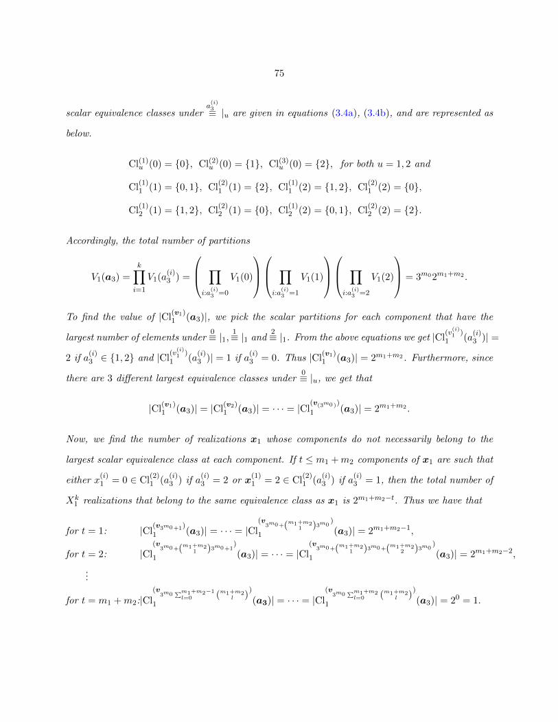
75

scalar equivalence classes undera(i)3≡ |u are given in equations (3.4a), (3.4b), and are represented as

below.

Cl(1)u (0) = {0}, Cl(2)

u (0) = {1}, Cl(3)u (0) = {2}, for both u = 1, 2 and

Cl(1)1 (1) = {0, 1}, Cl

(2)1 (1) = {2}, Cl

(1)1 (2) = {1, 2}, Cl

(2)1 (2) = {0},

Cl(1)2 (1) = {1, 2}, Cl

(2)2 (1) = {0}, Cl

(1)2 (2) = {0, 1}, Cl

(2)2 (2) = {2}.

Accordingly, the total number of partitions

V1(a3) =k∏i=1

V1(a(i)3 ) =

∏i:a

(i)3 =0

V1(0)

∏i:a

(i)3 =1

V1(1)

∏i:a

(i)3 =2

V1(2)

= 3m02m1+m2 .

To find the value of |Cl(v1)1 (a3)|, we pick the scalar partitions for each component that have the

largest number of elements under0≡ |1,

1≡ |1 and2≡ |1. From the above equations we get |Cl

(v(i)1 )

1 (a(i)3 )| =

2 if a(i)3 ∈ {1, 2} and |Cl

(v(i)1 )

1 (a(i)3 )| = 1 if a

(i)3 = 0. Thus |Cl

(v1)1 (a3)| = 2m1+m2. Furthermore, since

there are 3 different largest equivalence classes under0≡ |u, we get that

|Cl(v1)1 (a3)| = |Cl

(v2)1 (a3)| = · · · = |Cl

(v(3m0 ))

1 (a3)| = 2m1+m2 .

Now, we find the number of realizations x1 whose components do not necessarily belong to the

largest scalar equivalence class at each component. If t ≤ m1 +m2 components of x1 are such that

either x(i)1 = 0 ∈ Cl

(2)1 (a

(i)3 ) if a

(i)3 = 2 or x

(1)1 = 2 ∈ Cl

(2)1 (a

(i)3 ) if a

(i)3 = 1, then the total number of

Xk1 realizations that belong to the same equivalence class as x1 is 2m1+m2−t. Thus we have that

for t = 1: |Cl(v3m0+1)

1 (a3)| = · · · = |Cl(v

3m0+(m1+m21 )3m0

)

1 (a3)| = 2m1+m2−1,

for t = 2: |Cl(v

3m0+(m1+m21 )3m0+1

)

1 (a3)| = · · · = |Cl(v

3m0+(m1+m21 )3m0+(m1+m2

2 )3m0)

1 (a3)| = 2m1+m2−2,

...

for t = m1 +m2:|Cl(v

3m0∑m1+m2−1l=0 (m1+m2

l ))

1 (a3)| = · · · = |Cl(v

3m0∑m1+m2l=0 (m1+m2

l ))

1 (a3)| = 20 = 1.

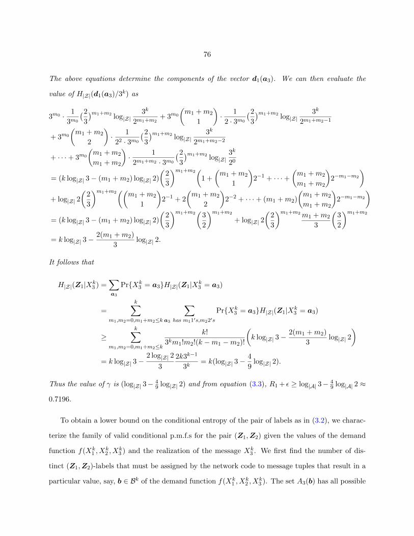
76

The above equations determine the components of the vector d1(a3). We can then evaluate the

value of H|Z|(d1(a3)/3k) as

3m0 · 1

3m0

(2

3

)m1+m2 log|Z|3k

2m1+m2+ 3m0

(m1 +m2

1

)· 1

2 · 3m0

(2

3

)m1+m2 log|Z|3k

2m1+m2−1

+ 3m0

(m1 +m2

2

)· 1

22 · 3m0

(2

3

)m1+m2 log|Z|3k

2m1+m2−2

+ · · ·+ 3m0

(m1 +m2

m1 +m2

)· 1

2m1+m2 · 3m0

(2

3

)m1+m2 log|Z|3k

20

= (k log|Z| 3− (m1 +m2) log|Z| 2)

(2

3

)m1+m2(

1 +

(m1 +m2

1

)2−1 + · · ·+

(m1 +m2

m1 +m2

)2−m1−m2

)+ log|Z| 2

(2

3

)m1+m2((

m1 +m2

1

)2−1 + 2

(m1 +m2

2

)2−2 + · · ·+ (m1 +m2)

(m1 +m2

m1 +m2

)2−m1−m2

)= (k log|Z| 3− (m1 +m2) log|Z| 2)

(2

3

)m1+m2(

3

2

)m1+m2

+ log|Z| 2

(2

3

)m1+m2m1 +m2

3

(3

2

)m1+m2

= k log|Z| 3−2(m1 +m2)

3log|Z| 2.

It follows that

H|Z|(Z1|Xk3 ) =

∑a3

Pr{Xk3 = a3}H|Z|(Z1|Xk

3 = a3)

=k∑

m1,m2=0,m1+m2≤k

∑a3 has m11′s,m22′s

Pr{Xk3 = a3}H|Z|(Z1|Xk

3 = a3)

≥k∑

m1,m2=0,m1+m2≤k

k!

3km1!m2!(k −m1 −m2)!

(k log|Z| 3−

2(m1 +m2)

3log|Z| 2

)

= k log|Z| 3−2 log|Z| 2

3

2k3k−1

3k= k(log|Z| 3−

4

9log|Z| 2).

Thus the value of γ is (log|Z| 3− 49 log|Z| 2) and from equation (3.3), R1 + ε ≥ log|A| 3− 4

9 log|A| 2 ≈

0.7196.

To obtain a lower bound on the conditional entropy of the pair of labels as in (3.2), we charac-

terize the family of valid conditional p.m.f.s for the pair (Z1,Z2) given the values of the demand

function f(Xk1 , X

k2 , X

k3 ) and the realization of the message Xk

3 . We first find the number of dis-

tinct (Z1,Z2)-labels that must be assigned by the network code to message tuples that result in a

particular value, say, b ∈ Bk of the demand function f(Xk1 , X

k2 , X

k3 ). The set A3(b) has all possible

77

realizations a3 of Xk3 that can result in the value of b for the demand function, i.e.,

A3(b) , {a3 ∈ Ak : ∃ x1,x2 ∈ Ak such that f(x1,x2,a3) = b}.

Let M(a3, b) denote the number of distinct (Z1,Z2) pair labels used for input message tuples

that have Xk3 = a3 and f(x1,x2,a3) = b. Consider two message tuples (x1,x2,a3) and (y1,y2,a3)

which satisfy f(x1,x2,a3) = f(y1,y2,a3) = b. If either x1

a3

6≡ y1|1 or x2

a3

6≡ y2|2, then the pair of

labels (Z1,Z2) assigned to the two message tuples must be different. This motivates us to define

the pair index set:

V12(a3, b) ,

(Cl(vj)1 ,Cl

(wt)2 ) :

∃ x1 ∈ Cl(vj)1 (a3),x2 ∈ Cl

(wt)2 (a3) s.t. f(x1,x2,a3) = b,

for all 1 ≤ j ≤ V1(a3), 1 ≤ t ≤ V2(a3)

.

The above discussion then implies that M(a3, b) ≥ |V12(a3, b)|. By the definition, if (Cl(v)1 ,Cl

(w)2 ) ∈

V12(a3, b) then for every i ∈ {1, 2, . . . , k}, the pair of scalar equivalence classes (Cl(v(i))1 ,Cl

(w(i))2 ) ∈

V12(a(i)3 , b(i)).

Illustration 3 Consider block size k = 1 and a realization b = 0 of the demand function of

Table 3.1. In the previous illustration we evaluated that Cl(1)1 (1) = {0, 1}, Cl

(2)1 (1) = {2} and

Cl(1)2 (1) = {1, 2}, Cl

(2)2 (1) = {0}. Then we can evaluate that the pair index set V12(1, 0) =

{(Cl(1)1 ,Cl

(1)2 ), (Cl

(1)1 ,Cl

(2)2 ), (Cl

(2)1 ,Cl

(1)2 )}. Note that the pair (Cl

(2)1 ,Cl

(2)2 ) /∈ V12(1, 0) as the ele-

ments of that pair of equivalence classes do not result in the demand function value of 0, i.e.,

Cl(2)1 (1) = {2}, Cl

(2)2 (1) = {0} but for x1 = 2, x2 = 0, x3 = 1, f(x1, x2, x3) = 1 6= 0.

Thus in this case we have that |V12(1, 0)| = 3. The other pair index sets are given in Table 3.2.

We now explicitly derive a p.m.f. whose entropy is a lower bound to the conditional entropy

H(Z1,Z2|f(Xk1 , X

k2 , X

k3 ) = b, Xk

3 = a3). Let A123(b) ⊆ Ak × Ak × Ak contain all message tuples

that are present in the pre-image of the demand function value of b. We also let A123(b,a3) ⊆

A123(b) denote the subset of message tuples for which the realization of Xk3 is a3. Suppose that

(Cl(v)1 ,Cl

(w)2 ) ∈ V12(a3, b). The number of different message tuples that cause the membership of

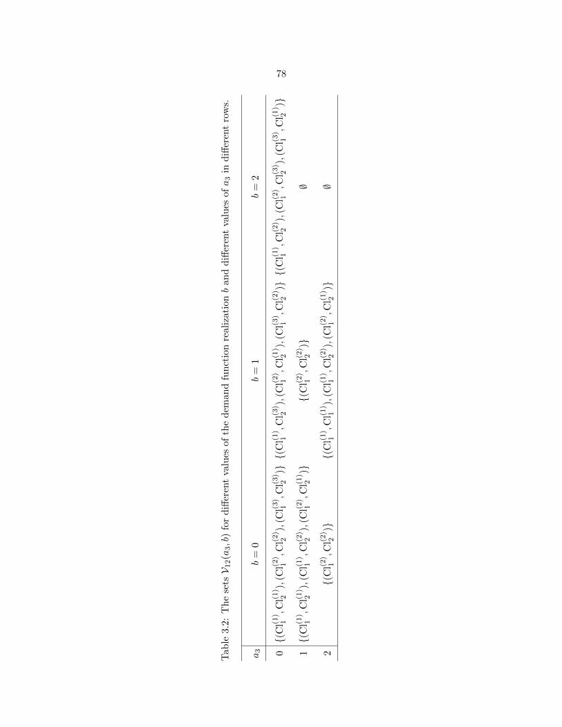
78

Tab

le3.

2:T

he

setsV 1

2(a

3,b

)fo

rd

iffer

ent

valu

esof

the

dem

and

fun

ctio

nre

aliz

atio

nb

and

diff

eren

tva

lues

ofa

3in

diff

eren

tro

ws.

a3

b=

0b

=1

b=

2

0{(

Cl(1

)1,C

l(1)

2),

(Cl(2

)1,C

l(2)

2),

(Cl(3

)1,C

l(3)

2)}{(

Cl(1

)1,C

l(3)

2),

(Cl(2

)1,C

l(1)

2),

(Cl(3

)1,C

l(2)

2)}{(

Cl(1

)1,C

l(2)

2),

(Cl(2

)1,C

l(3)

2),

(Cl(3

)1,C

l(1)

2)}

1{(

Cl(1

)1,C

l(1)

2),

(Cl(1

)1,C

l(2)

2),

(Cl(2

)1,C

l(1)

2)}

{(C

l(2)

1,C

l(2)

2)}

∅

2{(

Cl(2

)1,C

l(2)

2)}

{(C

l(1)

1,C

l(1)

1),

(Cl(1

)1,C

l(2)

2),

(Cl(2

)1,C

l(1)

2)}

∅

79

the equivalence class pair (Cl(v)1 ,Cl

(w)2 ) ∈ V12(a3, b) is denoted as follows.

ha3(v,w) ,∣∣∣{(x1,x2) : x1 ∈ Cl

(v)1 (a3),x2 ∈ Cl

(w)2 (a3), f(x1,x2,a3) = b}

∣∣∣ , (3.6)

= |Cl(v)1 (a3)| · |Cl

(w)2 (a3)|, (3.7)

=k∏i=1

|Cl(v(i))1 (a

(i)3 )| · |Cl

(w(i))2 (a

(i)3 )| =

k∏i=1

ha(i)3

(v(i), w(i)). (3.8)

Equality (3.7) is true above as by Definition 9 every element of an equivalence class undera3≡ |1

results in the same demand function value (while the other message x2 is held constant), and since

(Cl(v)1 ,Cl

(w)2 ) ∈ V12(a3, b), there is at least one x1 ∈ Cl

(v)1 (a3) and one x2 ∈ Cl

(w)2 (a3) such that

f(x1,x2,a3) = b. Hence every other pair of elements in Cl(v)1 (a3)×Cl

(w)2 (a3) would also result in

the same demand function value with Xk3 = a3.

Illustration 4 For block size k = 1 and demand function realization b = 0, we can check that

A3(0) = {0, 1, 2}. Following the indexing of the equivalence partitions and Table 3.2 we have that

h1(1, 1) = |Cl(1)1 (1)| · |Cl

(1)2 (1)| = 4 as Cl

(1)1 (1) = {0, 1} and Cl

(1)2 (1) = {1, 2}. One can similarly

check that h1(1, 2) = h1(2, 1) = 2 and for other values of a3, that h0(1, 1) = h0(2, 2) = h0(3, 3) = 1

and h2(2, 2) = 1.

For block size k = 3 and b = (1, 2, 1) we can check that a3 = (0, 0, 1) ∈ A3(b). Then the

equivalence class pairs under a3 that result in this b can be obtained in the following manner. If

(Cl(v)1 ,Cl

(w)2 ) ∈ V12(a3, b), then for each component, using Table 3.2 we have that

• (Cl(v(1))1 ,Cl

(w(1))2 ) ∈ V12(a

(1)3 , b(1)) = V12(0, 1) = {(Cl

(1)1 ,Cl

(3)2 ), (Cl

(2)1 ,Cl

(1)2 ), (Cl

(3)1 ,Cl

(2)2 )},

• (Cl(v(2))1 ,Cl

(w(2))2 ) ∈ V12(a

(2)3 , b(2)) = V12(0, 2) = {(Cl

(1)1 ,Cl

(2)2 ), (Cl

(2)1 ,Cl

(3)2 ), (Cl

(3)1 ,Cl

(1)2 )},

• (Cl(v(3))1 ,Cl

(w(3))2 ) ∈ V12(a

(3)3 , b(3)) = V12(1, 1) = {(Cl

(2)1 ,Cl

(2)2 )}.

As (Cl(v)1 ,Cl

(w)2 ) = (×3

i=1 Cl(v(i))1 ,×3

i=1 Cl(w(i))2 ), we get that |V12(a3, b)| = 9. One of these nine

equivalence class pairs is the pair (Cl((1,1,2))1 ,Cl

((3,2,2))2 ). Then using equation (3.8) we have that

h(0,0,1)((1, 1, 2), (3, 2, 2)) = h0(1, 3) · h0(1, 2) · h1(2, 2) = 1 · 1 · 1 = 1.

80

The proof of the following lemma is similar in spirit to that of Lemma 7.

Lemma 8 For any a3 ∈ A3(b), define the vector

hb,a3 ,

[ha3 ((v,w)1) ha3 ((v,w)2) · · · ha3

((v,w)|V12(a3,b)|

)0M(a3,b)−|V12(a3,b)|

]>,

where 0t indicates a vector of zeros of length t and subscript j in (v,w)j indexes all the equivalence

class pairs such that

ha3 ((v,w)1) ≥ ha3 ((v,w)2) ≥ · · · ≥ ha3

((v,w)|V12(a3,b)|

).

Then all conditional probability mass functions p ∈ RM(a3,b)≥0 on M(a3, b) valid (z1, z2)-labels given

the value b of the demand function and the realization a3 of Xk3 satisfy p ≺ hb,a3/|A123(b,a3)|.

It will be useful for analysis to define the following index sets of a demand function realization

b ∈ Bk and the message realization a3 ∈ A3(b).

Definition 10 For every p ∈ B, let Ip(b) ⊆ {1, 2, . . . , k} be the index set of components of the

demand function realization b that are equal to p, i.e.,

Ip(b) = {i : b(i) = p, i ∈ {1, 2, . . . , k}}.

We can similarly define the index set Jq(x3) for every q ∈ A.

Illustration 5 We evaluate H(hb,a3/|A123(b,a3)|) for a general block length k of the example

demand function. To specify hb,a3, we need to find |V12(a3, b)| and ha3((v,w)j) for all j ∈

{1, 2, . . . , |V12(a3, b)|}. Suppose the realization b ∈ {0, 1, 2}k has m1 1’s, m2 2’s and k −m1 −m2

0’s, and the realization of Xk3 is some a3 ∈ A3(b). Let tp,q for any p ∈ B, q ∈ A be defined as

tp,q , |Ip(b) ∩ Jq(a3)|. Note that t2,1 = t2,2 = 0 for any choice of b and a3.

|V12(a3, b)| We find the number of non-zero components of hb,a3, i.e. |V12(b,a3)|, as follows.

For every (Cl(v)1 ,Cl

(w)2 ) ∈ V12(a3, b), we have from Table 3.2 that for the index i,

• if i ∈ (I0(b) ∩ J2(a3)) ∪ (I1(b) ∩ J1(a3)), there is only one possible choice for the scalar

equivalence class pair (Cl(v(i))1 ,Cl

(w(i))2 ),

81

• else if i is not in the previous index set, then there are three possible choices for the scalar

equivalence class pair (Cl(v(i))1 ,Cl

(w(i))2 ).

Thus the total number of equivalence class pairs for for the choice of b and a3 is |V12(a3, b)| =

3k−t0,2−t1,1. Next we evaluate the components of the vector hb,a3.

ha3((v,w)1) Based on the subscript indexing of the pair (v,w) and equation (3.8), the value

of ha3((v,w)1) is obtained by counting the number of message tuples in the equivalence class pair

that has the largest scalar equivalence class pair for each component. As evaluated in the previous

illustration, the largest equivalence class pair for every i ∈ I0(b)∩J1(a3) has h1(1, 1) = 4 message

tuples, and for every i ∈ I1(b)∩J2(a3) the largest equivalence class again has h2(1, 1) = 4 message

tuples. For all other values of i, the largest equivalence class has a single input tuple. Hence we

have that ha3((v,w)1) = 4t0,1+t1,2. Note that there are three different choices for the largest scalar

equivalence class when i belongs to one of the following sets.

• i ∈ I0(b) ∩ J0(a3): there are t0,0 = k −m1 −m2 − t0,1 − t0,2 such components,

• i ∈ I1(b) ∩ J0(a3): there are t1,0 = m1 − t1,1 − t1,2 such components, and

• i ∈ I2(b) ∩ J0(a3): there are t2,0 = m2 such components.

Thus there are 3k−m1−m2−t0,1−t0,2 · 3m1−t1,1−t1,2 · 3m2 = 3k−t0,1−t0,2−t1,1−t1,2 components of hb,a3

which have the same value. Let k′ , k − t0,1 − t0,2 − t1,1 − t1,2. Hence we have that

ha3((v,w)1) = ha3((v,w)2) = · · · = ha3((v,w)3k′ ) = 4t0,1+t1,2 .

ha3((v,w)c) for c > 3k′

Next we consider the case when not every component of a message

tuple (x1,x2) ∈ Cl(v)1 × Cl

(w)2 is present in the largest scalar equivalence class pair. Suppose that

(Cl(v)1 ,Cl

(w)2 ) is such that

• at u0 indices from I0(b)∪J1(a3), the equivalence class pair is either (Cl(1)1 ,Cl

(2)2 ) or (Cl

(2)1 ,Cl

(1)2 ),

and

• at u1 indices from I1(b)∪J2(a3), the equivalence class pair is either (Cl(1)1 ,Cl

(2)2 ) or (Cl

(2)1 ,Cl

(1)2 ).

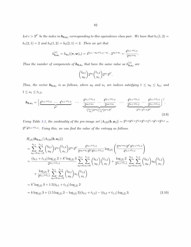
82

Let c > 3k′

be the index in hb,a3 corresponding to this equivalence class pair. We have that h1(1, 2) =

h1(2, 1) = 2 and h2(1, 2) = h2(2, 1) = 2. Then we get that

h(c)b,a3

= ha3((v,w)c) = 4t0,1−u0+t1,2−u1 · 2u0+u1 =4t0,1+t1,2

2u0+u1.

Thus the number of components of hb,a3 that have the same value as h(c)b,a3

are(t0,1u0

)2u0(t1,2u1

)2u13k

′.

Thus, the vector hb,a3 is as follows, where u0 and u1 are indices satisfying 1 ≤ u0 ≤ t0,1 and

1 ≤ u1 ≤ t1,2.

hb,a3 =[

4t0,1+t1,2 · · · 4t0,1+t1,2︸ ︷︷ ︸3k′

· · · 4t0,1+t1,2

2u0+u1· · · 4t0,1+t1,2

2u0+u1︸ ︷︷ ︸(t0,1u0 )2u0(t1,2u1 )2u13k′

· · · 4t0,1+t1,2

2t0,1+t1,2· · · 4t0,1+t1,2

2t0,1+t1,2︸ ︷︷ ︸2t0,12t1,23k′

]>.

(3.9)

Using Table 3.1, the cardinality of the pre-image set |A123(b,a3)| = 3t0,08t0,11t0,23t1,01t1,18t1,23t2,0 =

3k′8t0,1+t1,2. Using this, we can find the value of the entropy as follows.

H|Z|(hb,a3/|A123(b,a3)|)

=

t0,1∑u0=0

t1,2∑u1=0

(t0,1u0

)2u0(t1,2u1

)2u13k

′ 4t0,1+t1,2

2u0+u13k′8t0,1+t1,2log|Z|

(2u0+u13k

′8t0,1+t1,2

4t0,1+t1,2

)

=(t0,1 + t1,2) log|Z| 2 + k′ log|Z| 3

2t0,1+t1,2

t0,1∑u0=0

t1,2∑u1=0

(t0,1u0

)(t1,2u1

)+

log|Z| 2

2t0,1+t1,2

t0,1∑u0=0

t1,2∑u1=0

(t0,1u0

)u0

(t1,2u1

)

+log|Z| 2

2t0,1+t1,2

t0,1∑u0=0

t1,2∑u1=0

(t0,1u0

)u1

(t1,2u1

)= k′ log|Z| 3 + 1.5(t0,1 + t1,2) log|Z| 2

= k log|Z| 3 + (1.5 log|Z| 2− log|Z| 3)(t0,1 + t1,2)− (t0,2 + t1,1) log|Z| 3. (3.10)

83

3.3.2 Value of α

Having evaluated H(hb,a3/|A123(b,a3)|), we can find the value of α as used in equation (3.2)

in the following manner.

H(Z1,Z2|f(Xk1 , X

k2 , X

k3 ), Xk

3 )

=∑b

Pr{f(Xk1 , X

k2 , X

k3 ) = b}

∑x3

Pr{Xk3 = x3|f(Xk

1 , Xk2 , X

k3 ) = b}H(Z1,Z2|f(Xk

1 , Xk2 , X

k3 ) = b, Xk

3 = x3)

≥∑b

Pr{f(Xk1 , X

k2 , X

k3 ) = b}

∑x3

Pr{Xk3 = x3|f(Xk

1 , Xk2 , X

k3 ) = b}H(hb,a3/|A123(b,a3)|) , αk.

(3.11)

The value of Pr{f(Xk1 , X

k2 , X

k3 ) = b} can be found from Table 3.1 and the i.i.d. uniform assumption

on the message tuples. The value of Pr{Xk3 = x3|f(Xk

1 , Xk2 , X

k3 ) = b} can be evaluated by finding

the ratio of the cardinalities of two pre-image sets, i.e., |A123(b,x3)|/|A123(b)|. We carry out this

computation for the illustrated demand function below.

Illustration 6 Consider a realization b with m1 1’s, m2 2’s and k −m1 −m2 0’s. Then we have

that Pr{f(Xk1 , X

k2 , X

k3 ) = b} = (4/9)m1(1/9)m2(4/9)k−m1−m2. The number of different demand

function realizations which have the same number of 1’s, 2’s and 0’s is(

km1,m2,k−m1−m2

). Consider

a realization a3 ∈ A3(b) of the message Xk3 . The number of message tuples that result in the

demand function value b and have their Xk3 realization as a3 is |A123(b,a3)| = 3k

′8t0,1+t1,2, as

evaluated in the previous illustration. The number of message tuples in the pre-image set A123(b)

can be evaluated using Table 3.1 as |A123(b)| = 12m13m212k−m1−m2 = 3k4k−m2. Because of the

uniform i.i.d. assumption, we have that

Pr{Xk3 = x3|f(Xk

1 , Xk2 ,X

k3 ) = b} =

|A123(b,a3)||A123(b)| =

3k′8t0,1+t1,2

3k4k−m2

= (1/4)k−m1−m2−t0,1−t0,2(2/3)t0,1(1/12)t0,2(1/4)m1−t1,1−t1,2(2/3)t1,2(1/12)t1,1 .

Using equations (3.11), (3.10) and the probabilities computed above, the value of α is found in

Appendix C to be

α =8

9log|Z| 2 +

4

12log|Z| 3. (3.12)

84

Using this value of α in equation (3.2), we get that

R1 +R2

2+ ε ≥

α+(

log|Z| 9− 89 log|Z| 4

)2 log|Z| |A|

=89 log|A| 2 + 1

3 log|A| 3 + 2 log|A| 3− 169 log|A| 2

2≈ 1.7725

2.

3.3.3 Example demand function: Arithmetic sum

Suppose the message alphabet is A = {0, 1}, such that the messages X1, X2, X3 are independent

bits each equally likely to be 0 or 1. The demand function f(X1, X2, X3) = X1 + X2 + X3 is the

sum of the messages over the real numbers, such that B = {0, 1, 2, 3}. This case of arithmetic sum

computation in the variable-length network code framework was considered in [49] and we recover

the results there in our general framework. For a given value of the arithmetic sum b ∈ {0, 1, 2, 3}k

the set A3(b) of valid realizations for Xk3 can be described as

A3(b) = {a3 ∈ {0, 1}k : a(i)3 = 0 if b(i) = 0 and a

(j)3 = 1 if b(j) = 3 for all i, j ∈ {1, 2, . . . , k}}.

We consider the equivalence relationa3≡ |1 for the arithmetic sum demand function. Then

x1a3≡ y1|1 ⇔ x1 = y1,

because if x1 6= y1 then for all x2 ∈ {0, 1}k we have that x1 + x2 + a3 6= y1 + x2 + a3. A

similar conclusion also holds true for thea3≡ |2 relation. Thus for both u = 1 and 2, we have

that |Cl(v)u (a3)| = 1 for any class index v and Vu(a3) = 2k. We use the alphabet Z = {0, 1} for

communication. The vector du(a3) defined in Lemma 7 satisfies du(a3) = 12k in this case, where

1t indicates a vector of ones with length t. Using this in equation (3.5), we obtain the value of γ as

γ =1

k

∑a3∈Ak

Pr{Xk3 = a3}H|Z|

(du(a3)

|A|k)

=1

k· k = 1,

and thus Ru + ε ≥ 1/ log|Z| |A| = 1.

For any value of Xk1 , X

k3 and f(Xk

1 , Xk2 , X

k3 ) the value of Xk

2 is fixed by Xk2 = f(Xk

1 , Xk2 , X

k3 )−

Xk1 −Xk

3 . Hence, for every (Cl(v)1 ,Cl

(w)2 ) ∈ V12(a3) there is exactly one message tuple whose Xk

1

and Xk2 belong to the equivalence classes Cl

(v)1 (a3) and Cl

(w)2 (a3) respectively. Thus we have that

ha3(v,w) = 1 for every a3 ∈ A3(b) and (Cl(v)1 ,Cl

(w)2 ) ∈ V12(a3, b).

85

Consider an arithmetic sum realization b with m0 0’s, m1 1’s, m2 2’s and k −m0 −m1 −m2 3’s.

Define tp,q , |Ip(b) ∩ Jq(a3)| for every p ∈ {0, 1, 2, 3} and q ∈ {0, 1}. Then for any choice of b

and a3 ∈ A3(b), t0,1 = t3,0 = 0. The cardinality of the pre-image set |A123(b,a3)| = 2t1,0+t2,1 =

2t1,0+m2−t2,0 . The value of the entropy H(hb,a3/|A123(b,a3)|) = t1,0 +m2− t2,0. From the function

definition, we can check that |A123(b)| = 3m1+m2 . Thus we have that

Pr{Xk3 = x3|f(Xk

1 , Xk2 , X

k3 ) = b} =

|A123(b,a3)||A123(b)| =

2t1,0+m2−t2,0

3m1+m2.

Then the value of α can be found as follows.

αk =∑b

Pr{f(Xk1 , X

k2 , X

k3 ) = b}

∑a3∈A3(b)

Pr{Xk3 = a3|f(Xk

1 , Xk2 , X

k3 ) = b}H(hb,a3/|A123(b,a3)|)

=∑b

Pr{f(Xk1 , X

k2 , X

k3 )=b}

m1∑t1,0=0

m2∑t2,0=0

m1!(2/3)t1,0(1/3)m1−t1,0

t1,0!(m1 − t1,0)!

m2!(2/3)m2−t2,0(1/3)t2,0

t2,0!(m2 − t2,0)!(t1,0+m2−t2,0)

=k∑

m1=0

k−m1∑m2=0

k!2k−m1−m2

m1!m2!(k −m1 −m2)!

(1

8

)k−m1−m2(

3

8

)m1+m2 2(m1 +m2)

3

=2/3

4k

k∑m1=0

k−m1∑m2=0

k!(m1 +m2)

m1!m2!(k −m1 −m2)!

(3

2

)m1+m2

=2/3

4k2 · 3

2k4k−1 = 0.5k.

Putting this value of α in equation (3.2), we get that

R1 +R2

2+ ε ≥ 0.5 + 3− 0.75 log 3

2≈ 2.31128

2.

We note that the lower bound for the sum rate shown above is tighter than the bound R1+R2 > 2.25

obtained in [49] for the same problem. The inequalities considered there were similar to those used

in arriving at the sum rate lower bound in equation (3.2), however, in [49] they did not include Xk3

in the conditioning while lower bounding H|Z|(Z1,Z2|f(Xk1 , X

k2 , X

k3 )) as done here. Instead, they

directly lower bounded H|Z|(Z1,Z2|f(Xk1 , X

k2 , X

k3 )) using a so-called clumpy distribution, which is

a p.m.f. that majorizes any valid conditional p.m.f. of the pair (Z1,Z2) given f(Xk1 , X

k2 , X

k3 ). Since

only a lower bound to the entropy of the clumpy distribution was obtained in [49], the corresponding

lower bound for the sum rate ends up being looser than the value we obtain here. In the following,

we show that for k →∞, conditioning on Xk3 does not cause the bound to be any more looser than

86

that obtained by directly bounding H|Z|(Z1,Z2|f(Xk1 , X

k2 , X

k3 )) using the entropy of the clumpy

distribution.

We first describe a family P of p.m.f.s that must contain the conditional p.m.f.

Pr(Z1,Z2|f(Xk1 , X

k2 , X

k3 )) for any valid labelling scheme.

Lemma 9 Let L12(b) be the number of distinct (z1, z2) labels used by a valid labelling scheme

when Xk1 , X

k2 , X

k3 are such that f(Xk

1 , Xk2 , X

k3 ) = b. That implies L12(b) ≥M(a3, b) and we define

hb,a3 ,[h>b,a3

0L12(b)−M(a3,b)

]>for every a3 ∈ A3(b). The set of all conditional probability mass

functions on L12(b) labels given the function value b can be represented by a family P of vectors

over non-negative reals as below.

P =

p ∈ RL12(b)≥0 : p =

1

|A123(b)|∑

a3∈A3(b)

ga3 , where each ga3 ∈ ZL12(b)≥0 and ga3 ≺ hb,a3

.

Proof: In what follows, by distinct labels we mean distinct (z1, z2)-pair labels. By definitions

of the relevant quantities, there are L12(b) distinct labels that are assigned to the message tuples in

A123(b) and message tuples in A123(b,a3) for any a3 ∈ A3(b) are assigned M(a3, b) distinct labels.

However, for two different a3,a′3 ∈ A3(b), a label assigned to a message tuple in A123(b,a3) can

potentially be also assigned to a message tuple in A123(b,a′3). Since all messages are equally likely,

the conditional probability of observing a particular label then depends on how many message

tuples the label is assigned to across all A123(b,a3)-partitions (for all a3 ∈ A3(b)) of A123(b).

Each component of the vector p denotes the conditional probability of a distinct (z1, z2)-label

given the value b of the demand function. We define the non-negative integer vector ga3 as follows.

The lth component of ga3 , i.e., g(l)a3 records the number of message tuples in A123(b,a3) that are

assigned the (z1, z2) label corresponding to the lth component of p. Thus each component of the

sum∑

a3∈A3(b) ga3 describes the number of message tuples in the pre-image set A123(b) that are

assigned the label corresponding to that component. The conditional p.m.f. of (Z1,Z2) given

the function value b is obtained by dividing the sum by the cardinality of the pre-image set, i.e.,

|A123(b)|.

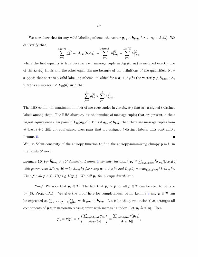
87

We now show that for any valid labelling scheme, the vector ga3 ≺ hb,a3 for all a3 ∈ A3(b). We

can verify thatL12(b)∑j=1

g(j)a3 = |A123(b,a3)| =

M(a3,b)∑l=1

h(l)b,a3

=

L12(b)∑j=1

h(j)b,a3

,

where the first equality is true because each message tuple in A123(b,a3) is assigned exactly one

of the L12(b) labels and the other equalities are because of the definitions of the quantities. Now

suppose that there is a valid labelling scheme, in which for a a3 ∈ A3(b) the vector g 6≺ hb,a3 , i.e.,

there is an integer t < L12(b) such that

t∑j=1

g[j]a3 >

t∑j=1

h[j]b,a3

.

The LHS counts the maximum number of message tuples in A123(b,a3) that are assigned t distinct

labels among them. The RHS above counts the number of message tuples that are present in the t

largest equivalence class pairs in V12(a3, b). Thus if ga3 ⊀ hb,a3 then there are message tuples from

at least t + 1 different equivalence class pairs that are assigned t distinct labels. This contradicts

Lemma 6.

We use Schur-concavity of the entropy function to find the entropy-minimizing clumpy p.m.f. in

the family P next.

Lemma 10 For hb,a3 and P defined in Lemma 9, consider the p.m.f. p? ,∑

a3∈A3(b) hb,a3/|A123(b)|

with parameters M?(a3, b) = V12(a3, b) for every a3 ∈ A3(b) and L?12(b) = maxa3∈A3(b)M?(a3, b).

Then for all p ∈ P, H(p) ≥ H(p?). We call p? the clumpy distribution.

Proof: We note that p? ∈ P. The fact that p? � p for all p ∈ P can be seen to be true

by [48, Prop. 6.A.1]. We give the proof here for completeness. From Lemma 9 any p ∈ P can

be expressed as∑

a3∈A3(b)ga3

|A123(b)| with ga3 ≺ hb,a3 . Let π be the permutation that arranges all

components of p ∈ P in non-increasing order with increasing index. Let p↓ , π(p). Then

p↓ = π(p) = π

(∑a3∈A3(b) ga3

|A123(b)|

)=

∑a3∈A3(b) π(ga3)

|A123(b)| ,

88

so p↓ ∈ P as ga3 ≺ hb,a3 implies that π(ga3) ≺ hb,a3 for any permutation π. Then p? � p↓, as for

any l ∈ L12(b),

l∑i=1

(p

[i]? − p[i]

↓

)=

l∑i=1

(p

(i)? − p(i)

↓

)=

1

|A123(b)|l∑

i=1

∑a3∈A3(b)

h(i)b,a3−

∑a3∈A3(b)

g(π−1(i))a3

,

=1

|A123(b)|l∑

i=1

∑a3∈A3(b)

{h

(i)b,a3− g(π−1(i))

a3

} =1

|A123(b)|∑

a3∈A3(b)

(l∑

i=1

{h

(i)b,a3− g(π−1(i))

a3

})≥ 0,

where the inequality above is again due to the fact that ga3 ≺ hb,a3 implies that π(ga3) ≺ hb,a3

for any permutation π. Since the majorization relation is a preordering and p? � p↓ � p, we get

that p? � p for any p ∈ P. As the entropy function is strictly Schur-concave, H(p) ≥ H(p?), with

equality if and only if p is a permutation of p?.

The number of distinct labels used for message tuples in A123(b,a3) is equal to the number

of positive components of hb,a3 . Thus M?(a3, b) = |V12(a3, b)| for all a3 ∈ A3(b) and the total

number of non-zero entries of p?, which is the same as the number of distinct labels used for all

the message tuples in A123(b) is L?12(b) = maxa3∈A3(b)M?(a3, b).

We use (C1,C2) to denote the codewords whose conditional p.m.f. given the demand function value

b is the clumpy distribution, i.e., Pr{C1,C2|f(Xk1 , X

k2 , X

k3 ) = b} = p?. From the definition of p?

and P, we have that H(C1,C2|f(Xk1 , X

k2 , X

k3 ) = b, Xk

3 = a3) = H(hb,a3/|A123(b,a3)|). Using the

definition of α in Eq. (3.11) and noting that H(hb,a3/|A123(b)|) = H(hb,a3/|A123(b)|), we get that

H(C1,C2|f(Xk1 , X

k2 , X

k3 ), Xk

3 ) = αk. Then we have the following.

(H|Z|(Z1) +H|Z|(Z2))/k ≥ H|Z|(f(Xk1 , X

k2 , X

k3 ))/k +H|Z|(Z1,Z2|f(Xk

1 , Xk2 , X

k3 ))/k

≥ H|Z|(f(Xk1 , X

k2 , X

k3 ))/k +H|Z|(C1,C2|f(Xk

1 , Xk2 , X

k3 ))/k

= H|Z|(f(Xk1 , X

k2 , X

k3 ))/k +H|Z|(C1,C2|f(Xk

1 , Xk2 , X

k3 ), Xk

3 )/k

+ I|Z|(C1,C2;Xk3 |f(Xk

1 , Xk2 , X

k3 ))/k

→ H|Z|(f(Xk1 , X

k2 , X

k3 ))/k + α+ I|Z|(C1,C2;Xk

3 |f(Xk1 , X

k2 , X

k3 ))/k

as k →∞.

Next, we show that when f(Xk1 , X

k2 , X

k3 ) is the arithmetic sum function,

I|Z|(C1,C2;Xk3 |f(Xk

1 , Xk2 , X

k3 ))/k → 0 as k →∞.

89

Definition 11 For p ∈ {0, 1, 2, 3} and q ∈ {0, 1}, define the random variable

Tp,q(Xk3 , f(Xk

1 , Xk2 , X

k3 )) = |Ip(f(Xk

1 , Xk2 , X

k3 )) ∩ Jq(Xk

3 )|.

For arithmetic sum, we have that T0,1(Xk3 , f(Xk

1 , Xk2 , X

k3 )) = T3,0(Xk

3 , f(Xk1 , X

k2 , X

k3 )) = 0.

Conditioned on a particular value of the arithmetic sum, say b, both T1,0(·) and T2,1(·) follow the

Binomial distribution. Suppose b has m1 1’s and m2 2’s. Then we have that

Pr{T1,0(Xk3 , f(Xk

1 , Xk2 , X

k3 )) = t1,0|f(Xk

1 , Xk2 , X

k3 ) = b}

=

(m1

t1,0

)Pr(X3 = 0|f(X1, X2, X3) = 1)t1,0 Pr(X3 = 1|f(X1, X2, X3) = 1)m1−t1,0

=

(m1

t1,0

)(2

3

)t1,0(1

3

)m1−t1,0,

Pr{T2,1(Xk3 , f(Xk

1 , Xk2 , X

k3 )) = t2,1|f(Xk

1 , Xk2 , X

k3 ) = b}

=

(m2

t2,1

)Pr(X3 = 1|f(X1, X2, X3) = 2)t2,1 Pr(X3 = 0|f(X1, X2, X3) = 2)m2−t2,1

=

(m2

t2,1

)(2

3

)t2,1(1

3

)m2−t2,1.

For either p = 1 or 2, consider the random source {X(j)3 ∈ A : j ∈ Ip(b), f(Xk

1 , Xk2 , X

k3 ) = b}, and

define its strongly δ-typical set [54, Chap. 5] as containing all vectors x3 ∈ A|Ip(b)| which satisfy

the following:

if p = 1 :

∣∣∣∣#(0;x3)

m1− 2

3

∣∣∣∣+

∣∣∣∣#(1;x3)

m1− 1

3

∣∣∣∣ ≤ δ=⇒

∣∣∣∣#(0;x3)

m1− 2

3

∣∣∣∣+

∣∣∣∣m1 −#(0;x3)

m1− 1

3

∣∣∣∣ = 2

∣∣∣∣#(0;x3)

m1− 2

3

∣∣∣∣ ≤ δ, (3.13a)

or if p = 2 :

∣∣∣∣#(0;x3)

m2− 1

3

∣∣∣∣+

∣∣∣∣#(1;x3)

m2− 2

3

∣∣∣∣ ≤ δ=⇒

∣∣∣∣m2 −#(1;x3)

m2− 1

3

∣∣∣∣+

∣∣∣∣#(1;x3)

m2− 2

3

∣∣∣∣ = 2

∣∣∣∣#(1;x3)

m2− 2

3

∣∣∣∣ ≤ δ, (3.13b)

where #(q;x3) for q ∈ {0, 1} counts the components in the vector x3 that are equal to q.

Lemma 11 For the arithmetic sum function, I(C1,C2;Xk3 |f(Xk

1 , Xk2 , X

k3 ))/k → 0 as k →∞.

Proof: Let E denote the event in which the sources {X(j)3 ∈ A : j ∈ Ip(b), f(Xk

1 , Xk2 , X

k3 ) =

b} for p = 1 and 2 both belong to their respective strongly δ-typical sets, and 1{E} be its indicator

90

random variable. Let Tβ(f) denote the strongly β-typical set of the arithmetic sum f(Xk1 , X

k2 , X

k3 ).

Then we have the following.

I(Xk3 ;C1,C2|f(Xk

1 , Xk2 , X

k3 )) = I(Xk

3 ;C1,C2|f(Xk1 , X

k2 , X

k3 )) + I(1{E};C1,C2|f(Xk

1 , Xk2 , X

k3 ), Xk

3 )

= I(Xk3 ,1{E};C1,C2|f(Xk

1 , Xk2 , X

k3 ))

= I(1{E};C1,C2|f(Xk1 , X

k2 , X

k3 )) + I(Xk

3 ;C1,C2|f(Xk1 , X

k2 , X

k3 ),1{E})

≤ H(1{E}) +∑

b/∈Tβ(f)

Pr{f(Xk1 , X

k2 , X

k3 ) = b}I(C1,C2;Xk

3 |1{E}, f(Xk1 , X

k2 , X

k3 ) = b)

+∑

b∈Tβ(f)

Pr{f(Xk1 , X

k2 , X

k3 ) = b}I(C1,C2;Xk

3 |1{E}, f(Xk1 , X

k2 , X

k3 ) = b)

≤ 1 +∑

b/∈Tβ(f)

Pr{f(Xk1 , X

k2 , X

k3 ) = b}H(Xk

3 )

+∑

b∈Tβ(f)

Pr{f(Xk1 , X

k2 , X

k3 ) = b}Pr{1{E} = 0|f(Xk

1 , Xk2 , X

k3 ) = b}

· I(C1,C2;Xk3 |1{E} = 0, f(Xk

1 , Xk2 , X

k3 ) = b)

+∑

b∈Tβ(f)

Pr{f(Xk1 , X

k2 , X

k3 ) = b}Pr{1{E} = 1|f(Xk

1 , Xk2 , X

k3 ) = b}

· I(C1,C2;Xk3 |1{E} = 1, f(Xk

1 , Xk2 , X

k3 ) = b).

For a realization b ∈ Tβ(f), we have by definition of the strongly β-typical set∣∣∣∣ |I0(b)|k

− 1

8

∣∣∣∣+

∣∣∣∣m1

k− 3

8

∣∣∣∣+

∣∣∣∣m2

k− 3

8

∣∣∣∣+

∣∣∣∣ |I3(b)|k

− 1

8

∣∣∣∣ ≤ β,=⇒ k(3/8− β) ≤ m1 ≤ k(3/8 + β), k(3/8− β) ≤ m2 ≤ k(3/8 + β) and m1 +m2 ≤ 2k(3/8 + β).

Then for b ∈ Tβ(f) as k →∞, bothm1 →∞ andm2 →∞ and hence Pr(1{E} = 0|f(Xk1 , X

k2 , X

k3 ) =

b) ≤ δ2 + 2(1− δ)δ ≤ 2δ. Then we have

I(Xk3 ;C1,C2|f(Xk

1 , Xk2 , X

k3 ))

≤ 1 +∑

b/∈Tβ(f)

Pr{f(Xk1 , X

k2 , X

k3 ) = b}H(Xk

3 ) +∑

b∈Tβ(f)

Pr{f(Xk1 , X

k2 , X

k3 ) = b}2δH(Xk

3 )

+∑

b∈Tβ(f)

Pr{f(Xk1 , X

k2 , X

k3 ) = b,1{E} = 1}I(C1,C2;Xk

3 |1{E} = 1, f(Xk1 , X

k2 , X

k3 ) = b)

91

≤ 1 + βk log |A|+ 2δk log |A|

+∑

b∈Tβ(f)

Pr{1{E} = 1, f(Xk1 , X

k2 , X

k3 ) = b}

[H(C1,C2|1{E} = 1, f(Xk

1 , Xk2 , X

k3 ) = b)

−H(C1,C2|Xk3 ,1{E} = 1, f(Xk

1 , Xk2 , X

k3 ) = b)

].

Let AE3 (b) ⊆ A3(b) denote the set of realizations of Xk3 which result in the event E occurring.

Then for the clumpy distribution, we have that

H(C1,C2|1{E} = 1, f(Xk1 , X

k2 , X

k3 ) = b) = H

( ∑x3∈AE3 (b) hb,x3∑

x3∈AE3 (b) |A123(b,x3)|

),

H(C1,C2|Xk3 ,1{E} = 1, f(Xk

1 , Xk2 , X

k3 ) = b) =

∑x3∈AE3 (b)

|A123(b,x3)|(∑

x3∈AE3 (b) |A123(b,x3)|)H(

hb,x3

|A123(b,x3)|

).

For the arithmetic sum, we have that |A123(b,a3)| = 2t1,02t2,1 and hb,a3 = 1|A123(b,a3)|. Hence we

get that

H

(hb,x3

|A123(b,x3)|

)= log |A123(b,x3)| = t1,0 + t2,1.

By equations (3.13a), (3.13b), for any b ∈ Tβ(f) and x3 ∈ AE3 (b), we have that 2|t1,0−2m1/3| ≤ δm1

and 2|t2,1 − 2m1/3| ≤ δm2. Then we have that

H

(∑x3∈AE3 (b) |A123(b,x3)|(hb,x3/|A123(b,x3)|)∑

x3∈AE3 (b) |A123(b,x3)|

)≤ max

x3∈AE3 (b)H

(hb,x3

|A123(b,x3)|

)≤ (m1 +m2)(2/3 + δ/2),∑

x3∈AE3 (b)

|A123(b,x3)|(∑

x3∈AE3 (b) |A123(b,x3)|)H(

hb,x3

|A123(b,x3)|

)≥ min

x3∈AE3 (b)H

(hb,x3

|A123(b,x3)|

)

≥ (m1 +m2)(2/3− δ/2).

Thus we have that

I(Xk3 ;C1,C2|f(Xk

1 , Xk2 , X

k3 ))

≤ 1 + βk log |A|+ 2δk log |A|+∑

b∈Tβ(f)

Pr(1{E} = 1, f(Xk1 , X

k2 , X

k3 ) = b)(m1 +m2)δ

≤ 1 + βk log |A|+ 2δk log |A|+∑

b∈Tβ(f)

Pr(1{E} = 1, f(Xk1 , X

k2 , X

k3 ) = b)2k(3/8 + β)δ

92

=⇒ I(Xk3 ;C1,C2|f(Xk

1 , Xk2 , X

k3 ))/k ≤ 1/k + β log |A|+ 2δ log |A|+ 2(3/8 + β)δ.

Choosing β → 0 and δ → 0 and consequently k →∞, gives us the result.

3.3.4 Example demand function: Sum over GF (2)

Suppose the messages X1, X2, X3 ∈ {0, 1} and the terminal wants to compute their finite field

sum over GF (2). For this demand function, we demonstrate that the outer bound to the rate region

is tight. We assume that the alphabet used for communication is Z = {0, 1}.

For X3 we have that 0 6≡ 1, and thus for a function g(Xk3 ) that returns the equivalence class

that Xk3 belongs to, we have that H(g(Xk

3 )) = k. Thus from Lemma 4 we get that R31 +R32 ≥ 1.

For Xu, u = 1 or 2, using the values of the finite field sum, we obtain the following partitions

0≡ |u : {0} ∪ {1} and1≡ |u : {0} ∪ {1}.

Thus, similar to the case of arithmetic sum (c.f. Section 3.3.3), for a GF (2)-sum realization b

and a3 ∈ A3(b), the equivalence classes satisfy |Cl(v)1 (a3)| = |Cl

(w)2 (x3)| = 1 for any class index v

or w and V1(a3) = V2(a3) = 2k. Thus the vector du(a3) defined in Lemma 7 is 12k , and hence

H(du(a3)/2k) = k, giving us the value of γ as

γ = 1 =⇒ Ru + ε ≥ 1.

For any value of Xk1 , X

k3 and f(Xk

1 , Xk2 , X

k3 ) the value of Xk

2 is fixed by Xk2 = f(Xk

1 , Xk2 , X

k3 ) −

Xk1 −Xk

3 , where the subtraction operations are also over GF (2). Hence we have that

ha3(v,w) = 1 for every a3 ∈ A3(b) and (Cl(v)1 ,Cl

(w)2 ) ∈ V12(a3, b).

We enumerate the different (X1, X2) pairs that result in b(i) for the realization a(i)3 in different cases

as below.

• If i ∈ I0(b) ∩ J0(a3): (X1, X2) ∈ {(0, 0), (1, 1)}.

• If i ∈ I0(b) ∩ J1(a3): (X1, X2) ∈ {(0, 1), (1, 0)}.

93

• If i ∈ I1(b) ∩ J0(a3): (X1, X2) ∈ {(0, 1), (1, 0)}.

• If i ∈ I1(b) ∩ J1(a3): (X1, X2) ∈ {(0, 0), (1, 1)}.

Since there are two choices in each case, we have that |A123(b,a3)| = 2k. Thus we have that

hb,a3/|A123(b,a3)| = 12k which gives the value of α as

α = 1 =⇒ (R1 +R2)/2 + ε ≥ (1 +H(f(Xk1 , X

k2 , X

k3 ))/k)/2 = (1 + k/k)/2 = 1.

We describe simple network code that allows t to compute the GF (2)-sum by carrying out the

operation Z1(Xk1 ,Z31(Xk

3 )) + Z2(Xk2 ,Z32(Xk

3 )). The codewords used are

Z31(Xk3 ) = Xk

3 , Z32(Xk3 ) = 0.

Z1(Xk1 ,Z31(Xk

3 )) = Xk1 +Xk

3 , Z2(Xk2 ,Z32(Xk

3 )) = Xk2 .

The sums computed above are component-wise over GF (2). Then E`(Z31) = k,E`(Z32) = 0 and

E`(Z2) = k. If X1, X3 ∼ Unif{0, 1} then X1 + X3 ∼ Unif{0, 1}. Hence E`(Z1) = k. These imply

that the rate tuple achieved is

(R31, R32, R1, R2) = (1, 0, 1, 1),

which match the lower bounds derived above.

3.4 Conclusions and future work

In this paper, we have described a procedure to obtain an outer bound for the rate region

(in the setup of [50]) for computing a function with zero-error over a simple DAG network. The

demand function can be an arbitrary discrete-valued function and only needs to be specified as

a function table. For computing the arithmetic sum of three bits, we show that the outer bound

obtained is tighter than the one in [49]. For computing the GF (2)-sum of three bits, we show that

the lower bounds for the rate tuple obtained using our procedure can also be achieved by a simple

network code. Our method uses the equivalence relations defined in [47] as adapted to the specific

DAG network considered here. Assuming a independent, uniform probability distribution for each

94

of the messages, we compute the probability that the messages belong to a particular equivalence

class. These are used in obtaining a lower bound to the conditional entropy of the descriptions

transmitted on the edges, which imply an outer bound to the rate region.

There are many opportunities for future work. An immediate question is to find the exact

rate region for computing the arithmetic sum over the DAG network considered here. This func-

tion computation problem has been instructive in characterizing the worst-case communication

necessary for computation, and we expect it to play a similar role in finding the rate region for

average-case communication scenario. Progress in this direction should give us insights in obtain-

ing outer bounds for the rate region for computing functions other than the arithmetic sum on

this network. A different direction is to consider function computation over other directed acyclic

graph networks. An interesting question is whether we can ‘overlay’ the probability information, in

a manner similar to as done here, on the various equivalence classes as given in [47] for an arbitrary

DAG network and demand function and obtain corresponding outer bounds on the rate region.

95

CHAPTER 4. CONCLUSIONS AND FUTURE WORK

In our study on computing functions over networks, we have demonstrated certain characteris-

tics of the general problem. We have done this by focusing on certain tractable problem instances.

Sum-networks are function computation instances in which we are interested in computing the

finite field sum of messages observed in a network. The significance of the capacity problem for

a sum-network is underscored by a known reduction in the literature, which relates whether a

multiple-unicast problem can be solved at rate = 1 to whether the computation capacity of an

appropriate sum-network is 1. Multiple-unicast is a very general communication problem in which

several source-terminal pairs communicate their respective messages over a shared network. Finding

the computation capacity of a general sum-network is a well-known hard problem. We were able

to find the computation capacity of an infinite family of sum-networks that were obtained using

incidence structures. Depending on the structure of the sum-network, the computation capacity of

a sum-network was seen to greatly depend on the characteristic of the finite field over which the

sum is computed.

Computing the arithmetic sum of three bits over the directed acyclic graph network considered

in Chapter 3 has served as an illuminating example for various reasons. It is the smallest network

which does not have a tree structure. The computation capacity of networks with a tree structure

is known in the literature. Nevertheless, the worst-case computation capacity for computing the

arithmetic sum over this specific non-tree network was known in the literature through a combi-

natorial argument. However, as we have shown, the average-case computation capacity for this

problem is still unknown. For the average-case, we worked in the framework of a source-network

code and consequently the quantity of interest is a rate-region ⊆ R4≥0. The inner bound to the rate

region demonstrates that we can compute the arithmetic sum by communicating less than what is

required in the worst-case scenario, as one would expect. The technique by which we arrive at the

96

outer bound to the rate region can also be applied to functions other than the arithmetic sum, as

was demonstrated.

Key ideas used in Chapter 2

• We used incidence structures to construct our sum-network problem instances. The symmetry

in the incidence structure then translated into a symmetry in the network structure.

• The incidence between points and blocks of the incidence structure allowed us to determine the

minimum amount of independent information that must be transmitted across the bottleneck

edges in the sum-network. It was equal to the rank of a particular 0-1 matrix, where the

rank was evaluated over the finite field over which the sum is to be computed. This gave us

a finite-field dependent upper bound to the computation capacity of the sum-networks.

• We used certain non-negative integer matrices to obtain network codes whose rate matched

the upper bound. The existence of these matrices was shown using necessary and sufficient

conditions for the existence of integral flows over a flow-network. For several families of

incidence structures, we could verify that they satisfied these conditions by double-counting

the number of 1’s in various submatrices of the associated incidence matrix.

• There are sum-networks whose computation capacity is 1 over a finite field but close to 0 over

a different finite field. This was established using existence results for balanced incomplete

block designs known in the literature.

Key ideas used in Chapter 3

• It is well-known that one can describe a sequence of independent and identically distributed

random variables using codeword whose expected length per symbol is asymptotically close

to the entropy of the random variable. We use this idea to find the length of the codewords

that are generated by the encoders at s1 and s2 in terms of the entropy of the codewords.

This allows us to reduce the average amount of communication required.

97

• It is known in the literature that communicating which equivalence class a message belongs

to is sufficient for correctly computing the function. Using this idea and applying the pigeon-

hole principle, we can specify a family of probability mass functions that must contain the

conditional probability mass function of the codewords given the function value and the

message observed at s3.

• A lower bound to the conditional entropy is found by evaluating the entropy of a probability

mass function that majorizes every other probability mass function in the family. This is

because of the Schur concave property of the entropy function. This lower bound is used to

get an outer bound to the rate region.

4.1 Future work

There are many avenues for future work within the general problem setup of this thesis for

computing functions over networks. Some of them were highlighted in the conclusion sections of

Chapters 2 and 3. Here we outline some other general directions of future work. For example, in the

case of computing the finite field sum, what methods could be used to find the computation capacity

of other sum-networks whose structure is not as symmetric as those obtained using incidence

structures. For the class of sum-networks constructed using our procedure, there exist sum-networks

for which we have an upper bound to the computation capacity but no network code with a matching

rate.

For the particular directed acyclic graph considered in Chapter 3, an immediate question is to

find the exact rate region for the computing arithmetic sum. This problem has been instructive

for finding the worst-case communication necessary for computation, and we expect it to play a

similar role in finding the average-case communication scenario. Progress in this direction should

give us insights for obtaining outer bounds for the rate region for computing functions other than

the arithmetic sum on this network.

98

BIBLIOGRAPHY

[1] J. Korner and K. Marton, “How to encode the modulo-2 sum of binary sources,” IEEE Trans.on Info. Th., vol. 25, no. 2, pp. 219–221, 1979.

[2] A. Orlitsky and J. Roche, “Coding for computing,” IEEE Trans. on Info. Th., vol. 47, no. 3,pp. 903–917, Mar 2001.

[3] V. Doshi, D. Shah, M. Medard, and M. Effros, “Functional compression through graph color-ing,” IEEE Trans. on Info. Th., vol. 56, no. 8, pp. 3901–3917, Aug 2010.

[4] R. Ahlswede, N. Cai, S.-Y. Li, and R. W. Yeung, “Network Information Flow,” IEEE Trans.on Info. Th., vol. 46, no. 4, pp. 1204–1216, 2000.

[5] R. Koetter and M. Medard, “An algebraic approach to network coding,” IEEE/ACM Trans-actions on Networking, vol. 11, no. 5, pp. 782–795, Oct 2003.

[6] S.-Y. R. Li, R. W. Yeung, and N. Cai, “Linear network coding,” IEEE Trans. on Info. Th.,vol. 49, no. 2, pp. 371–381, Feb 2003.

[7] R. Dougherty, C. Freiling, and K. Zeger, “Insufficiency of linear coding in network informationflow,” IEEE Trans. on Info. Th., vol. 51, no. 8, pp. 2745–2759, Aug. 2005.

[8] J. Cannons, R. Dougherty, C. Freiling, and K. Zeger, “Network routing capacity,” IEEE Trans.on Info. Th., vol. 52, no. 3, pp. 777–788, Mar. 2006.

[9] R. Dougherty, C. Freiling, and K. Zeger, “Unachievability of network coding capacity,” IEEETrans. on Info. Th., vol. 52, no. 6, pp. 2365–2372, June 2006.

[10] S. Jaggi, P. Sanders, P. A. Chou, M. Effros, S. Egner, K. Jain, and L. M. G. M. Tolhuizen,“Polynomial time algorithms for multicast network code construction,” IEEE Trans. on Info.Th., vol. 51, no. 6, pp. 1973–1982, June 2005.

[11] S. Huang and A. Ramamoorthy, “An achievable region for the double unicast problem basedon a minimum cut analysis,” IEEE Trans. on Comm., vol. 61, no. 7, pp. 2890–2899, 2013.

[12] S. Huang and A. Ramamoorthy, “On the multiple unicast capacity of 3-source, 3-terminaldirected acyclic networks,” IEEE/ACM Trans. on Networking, vol. 22, no.1, pp. 285–299,2014.

[13] A. R. Lehman and E. Lehman, “Complexity classification of network information flow prob-lems,” in Proceedings of the Fifteenth Annual ACM-SIAM Symposium on Discrete Algorithms,Jan 2004, pp. 142–150.

[14] S. Kamath, D. N. C. Tse, and C. C. Wang, “Two-unicast is hard,” in IEEE Intl. Symposiumon Info. Th., June 2014, pp. 2147–2151.

99

[15] R. Appuswamy, M. Franceschetti, N. Karamchandani, and K. Zeger, “Network coding forcomputing: Cut-set bounds,” IEEE Trans. on Info. Th., vol. 57, no. 2, pp. 1015–1030, Feb2011.

[16] C. Huang, Z. Tan, and S. Yang, “Upper bound on function computation in directed acyclicnetworks,” in IEEE Info. Th. Workshop, April 2015, pp. 1–5.

[17] R. Appuswamy, M. Franceschetti, N. Karamchandani, and K. Zeger, “Linear codes, targetfunction classes, and network computing capacity,” IEEE Trans. on Info. Th., vol. 59, no. 9,pp. 5741–5753, Sept 2013.

[18] A. Ramamoorthy, “Communicating the sum of sources over a network,” in IEEE Intl. Sympo-sium on Info. Th., July 2008, pp. 1646–1650.

[19] B. K. Rai and B. K. Dey, “On network coding for sum-networks,” IEEE Trans. on Info. Th.,vol. 58, no. 1, pp. 50 –63, 2012.

[20] A. Ramamoorthy and M. Langberg, “Communicating the sum of sources over a network,”IEEE J. Select. Areas Comm., vol. 31, no. 4, pp. 655–665, 2013.

[21] D. R. Stinson, Combinatorial Designs: Construction and Analysis. Springer, 2003.

[22] O. Olmez and A. Ramamoorthy, “Fractional repetition codes with flexible repair from combi-natorial designs,” IEEE Trans. on Info. Th., vol. 62, no. 4, pp. 1565 –1591, 2016.

[23] S. E. Rouayheb and K. Ramchandran, “Fractional repetition codes for repair in distributedstorage systems,” in 48th Annual Allerton Conference on Comm., Control & Computing, Sept2010, pp. 1510 –1517.

[24] L. Tang and A. Ramamoorthy, “Coded caching with low subpacketization levels,” in Intl.Symp. on Network Coding (NetCod), Dec 2016, pp. 1–6.

[25] L. Tang and A. Ramamoorthy, “Coded Caching Schemes with Reduced Subpacketization fromLinear Block Codes,” IEEE Trans. on Info. Th., vol. 64, no. 4, pp. 3099–3120, 2018.

[26] L. Tang and A. Ramamoorthy, “Coded caching for networks with the resolvability property,”in IEEE Intl. Symposium on Info. Th., July 2016, pp. 420-424.

[27] L. Tang and A. Ramamoorthy, “Low subpacketization schemes for coded caching,” in IEEEIntl. Symposium on Info. Th., June 2017, pp. 2790-2794.

[28] B. K. Rai and N. Das, “On the capacity of ms/3t and 3s/nt sum-networks,” in IEEE Info.Th. Workshop, Sep. 2013, pp. 1–5.

[29] B. Rai and N. Das, “On the capacity of sum-networks,” in 51st Annual Allerton Conferenceon Comm., Control & Computing, Oct 2013, pp. 1545–1552.

[30] A. Tripathy and A. Ramamoorthy, “Sum-networks from undirected graphs: Construction andcapacity analysis,” in 52nd Annual Allerton Conference on Comm., Control & Computing,Sept 2014, pp. 651–658.

100

[31] N. Das and B. K. Rai, “On the number of sources and terminals of sum-networks with capacityp/q,” in 21st National Conference on Communications (NCC), Feb 2015, pp. 1–6.

[32] A. Tripathy and A. Ramamoorthy, “Capacity of sum-networks for different message alpha-bets,” in IEEE Intl. Symposium on Info. Th., June 2015, pp. 606–610.

[33] R. A. Brualdi, Combinatorial matrix classes. Cambridge University Press, 2006, vol. 13.

[34] L. Mirsky, “Combinatorial theorems and integral matrices,” Journal of Combinatorial Theory,vol. 5, no. 1, pp. 30–44, 1968.

[35] L. Teirlinck, “Non-trivial t-designs without repeated blocks exist for all t,” Discrete Mathe-matics, vol. 65, no. 3, pp. 301–311, 1987.

[36] C. J. Colbourn and J. H. Dinitz, Handbook of combinatorial designs. CRC press, 2006.

[37] A. Giridhar and P. R. Kumar, “Computing and communicating functions over sensor net-works,” IEEE Journal on Selected Areas in Communications, vol. 23, no. 4, pp. 755-764, April2005.

[38] A. E. Gamal and Y.-H. Kim, Network Information Theory. Cambridge University Press, Jan2012.

[39] H. Witsenhausen, “The zero-error side information problem and chromatic numbers (Cor-resp.),” IEEE Trans. on Info. Th., vol. 22, no. 5, pp. 592-593, September 1976.

[40] N. Alon and A. Orlitsky, “Source coding and graph entropies,” IEEE Trans. on Info. Th.,vol. 42, no. 5, pp. 1329-1339, Sep 1996.

[41] J. Korner and A. Orlitsky, “Zero-error information theory,” IEEE Trans. on Info. Th., vol. 44,no. 6, pp. 2207-2229, Oct 1998.

[42] T. S. Han and K. Kobayashi, “A dichotomy of functions F (X,Y ) of correlated sources (X,Y )from the viewpoint of the achievable region,” IEEE Trans. on Info. Th., vol. 33, no. 1, pp.69-76, January 1987.

[43] S. Feizi and M. Medard, “On Network Functional Compression,” IEEE Trans. on Info. Th.,vol. 60, no. 9, pp. 5387-5401, Sept. 2014.

[44] M. Sefidgaran and A. Tchamkerten, “Distributed Function Computation Over a Rooted Di-rected Tree,” IEEE Trans. on Info. Th., vol. 62, no. 12, pp. 7135-7152, Dec. 2016.

[45] H. Kowshik and P. R. Kumar, “Optimal Function Computation in Directed and UndirectedGraphs,” IEEE Trans. on Info. Th., vol. 58, no. 6, pp. 3407–3418, June 2012.

[46] T. Cover and J. Thomas, Elements of Information Theory, ser. Wiley Series in Telecommuni-cations and Signal Processing. Wiley-Interscience, 2006.

[47] X. Guang, S. Yang, and C. Li, “An improved upper bound on network function computationusing cut-set partition,” in IEEE Info. Th. Workshop, Sept 2016, pp. 11–15.

101

[48] A. W. Marshall, I. Olkin, and B. C. Arnold, Inequalities: Theory of Majorization and ItsApplications, ser. Springer Series in Statistics. Springer New York, 2011.

[49] A. Tripathy and A. Ramamoorthy, “On computation rates for arithmetic sum,” in IEEE Intl.Symposium on Info. Th., July 2016, pp. 2354–2358.

[50] L. Song, R. W. Yeung and N. Cai, “Zero-error network coding for acyclic networks,” in IEEETrans. on Info. Th., vol. 49, no. 12, pp. 3129–3139, Dec. 2003.

[51] S. Leung-Yan-Cheong and T. Cover, “Some equivalences between Shannon entropy and Kol-mogorov complexity,” IEEE Trans. on Info. Th., vol. 24, no. 3, pp. 331–338, May 1978.

[52] X. Guang, R. W. Yeung, S. Yang and C. Li, “Improved upper bound on the network functioncomputing capacity,” online at http://arxiv.org/abs/1710.02252.

[53] K. Konstantinidis and A. Ramamoorthy, “Leveraging Coding Techniques for Speeding upDistributed Computing,” online at http://arxiv.org/abs/1802.03049.

[54] R. W. Yeung, A First Course in Information Theory, ser. Information Technology: Transmis-sion, Processing and Storage. Springer US, 2002.

[55] A. Tripathy and A. Ramamoorthy, “Sum-networks from incidence structures: constructionand capacity analysis,” IEEE Trans. on Info. Th., vol. 64, no. 5, pp. 3461–3480, May 2018.

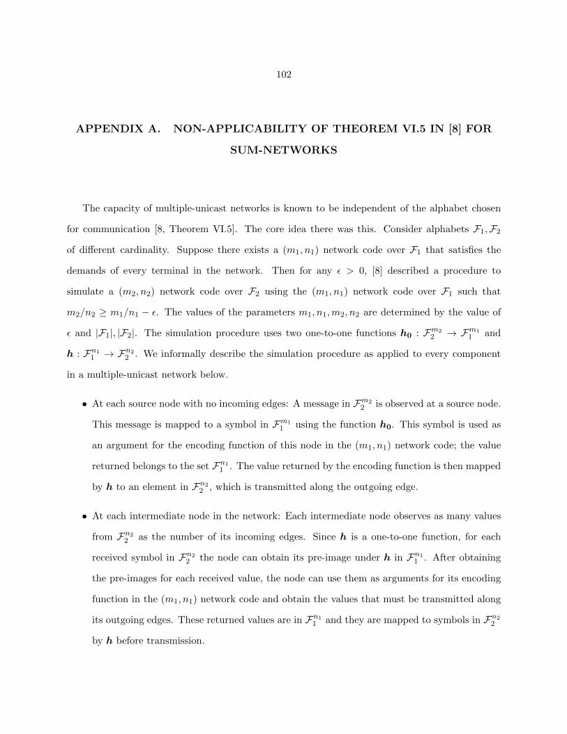
102

APPENDIX A. NON-APPLICABILITY OF THEOREM VI.5 IN [8] FOR

SUM-NETWORKS

The capacity of multiple-unicast networks is known to be independent of the alphabet chosen

for communication [8, Theorem VI.5]. The core idea there was this. Consider alphabets F1,F2

of different cardinality. Suppose there exists a (m1, n1) network code over F1 that satisfies the

demands of every terminal in the network. Then for any ε > 0, [8] described a procedure to

simulate a (m2, n2) network code over F2 using the (m1, n1) network code over F1 such that

m2/n2 ≥ m1/n1 − ε. The values of the parameters m1, n1,m2, n2 are determined by the value of

ε and |F1|, |F2|. The simulation procedure uses two one-to-one functions h0 : Fm22 → Fm1

1 and

h : Fn11 → Fn2

2 . We informally describe the simulation procedure as applied to every component

in a multiple-unicast network below.

• At each source node with no incoming edges: A message in Fm22 is observed at a source node.

This message is mapped to a symbol in Fm11 using the function h0. This symbol is used as

an argument for the encoding function of this node in the (m1, n1) network code; the value

returned belongs to the set Fn11 . The value returned by the encoding function is then mapped

by h to an element in Fn22 , which is transmitted along the outgoing edge.

• At each intermediate node in the network: Each intermediate node observes as many values

from Fn22 as the number of its incoming edges. Since h is a one-to-one function, for each

received symbol in Fn22 the node can obtain its pre-image under h in Fn1

1 . After obtaining

the pre-images for each received value, the node can use them as arguments for its encoding

function in the (m1, n1) network code and obtain the values that must be transmitted along

its outgoing edges. These returned values are in Fn11 and they are mapped to symbols in Fn2

2

by h before transmission.

103

s1 s2t

e1 e2

Figure A.1: A simple sum-network. Both edges can transmit one symbol in F1 from tail to headin one channel use.

• Decoding at each terminal node in the network: At each terminal node, the received values in

Fn22 are mapped to their pre-images in Fn1

1 under h. These pre-images are used as arguments

for the decoding function of this terminal in the (m1, n1) network code. The value returned

by the decoding function is an element of Fm11 that is the image under h0 of the demanded

message at this terminal. Since h0 is also a one-to-one function, each terminal can recover

its required message.

This simulation procedure however cannot be applied to sum-networks as is illustrated by the

example below.

Example 13 Consider a simple sum-network shown in Figure A.1, terminal t wants to evaluate

X1 +X2 where X1, X2 ∈ F1 are random variables observed at source nodes s1, s2 respectively. We

have a scalar network code (rate = 1) that satisfies the problem, described as follows.

1. Edge functions:

φe1(X1) = X1, φe2(X2) = X2.

2. Decoding function:

ψ(φe1(X1), φe2(X2)) = φe1(X1) + φe2(X2) = X1 +X2

and X1 +X2 is the only value terminal t is interested in decoding.

We use the procedure outlined in [8] to extend the network code for another alphabet F2. Let

F1 = GF (3),F2 = GF (2). Setting ε = 21−γ/ log2 3 where γ > 1, we obtain the following values

m1 = n1 = d2γe , n2 =

⌈2γ

log2 3

⌉and m2 = n2 − 1.

104

Let h0 : F2 → F1 be such that

h0(x) =

0 if x = 0,

1 if x = 1.

and let h0 : F1 → F2 be such that h0(h0(x)) = x for all x ∈ F2 and arbitrary otherwise. Then we

can define an injection h0 : Fm22 → Fm1

1 as the component-wise application of h0 to each of the

elements in the argument.

h0(b1, b2, . . . , bm2) =

[h0(b1) h0(b2) . . . h0(bm2) 0m1−m2

]where b1, b2, . . . bm2 ∈ F2 and 0m1−m2 is a zero vector with m1 − m2 components. We define

h0 : Fm11 → Fm2

2 as

h0(a1, a2, . . . , am1) =

[h0(a1) h0(a2) . . . h0(am2)

]where a1, a2, . . . , am1 ∈ F1.

Also we let h : Fn11 → Fn2

2 be an arbitrary injection and h : Fn22 → Fn1

1 is such that h(h(x)) =

x for all x ∈ Fn11 and arbitrary otherwise. This is possible because 3d2

γe ≥ 2d2γ/ log2 3e for any

γ > 1. We now use the extended network code to satisfy the sum network for when the source

random variables take values in the alphabet Fm22 . Suppose a particular realization of X1 ∈ Fm2

2

and X2 ∈ Fm22 is such that

x1 = (1, 1, . . . , 1) = 1m2 and x2 = (1, 1, . . . , 1) = 1m2 .

Following steps in [8] for the decoding function we get that terminal t carries out the following

operation to obtain the value of x1 + x2

h0(ψt(φe1(h0(x1)), φe2(h0(x2)))) = h0(h0(x1) + h0(x2))

= h0([1m2 0m1−m2 ] + [1m2 0m1−m2 ])

= h0([2m2 0m1−m2 ])

where 2m2 is a vector of m2 2’s.

105

Since h0(2) is arbitrarily assigned, h0([2m2 0m1−m2 ]) need not equal 0m2 which is the right

value of x1 +x2. Thus the simulated (m2, n2) network code over F2 does not correctly evaluate the

required sum.

In fact, the computation capacity of sum-networks explicitly depends on the alphabet used in

message generation and communication, as described in Sections 2.5, 2.6. Moreover, the choice of

alphabet can significantly reduce the computation capacity of the same sum-network as discussed

in Section 2.7.

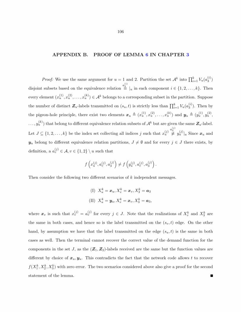
106

APPENDIX B. PROOF OF LEMMA 6 IN CHAPTER 3

Proof: We use the same argument for u = 1 and 2. Partition the set Ak into∏ki=1 Vu(a

(i)3 )

disjoint subsets based on the equivalence relationa(i)3≡ |u in each component i ∈ {1, 2, . . . , k}. Then

every element (x(1)u , x

(2)u , . . . , x

(k)u ) ∈ Ak belongs to a corresponding subset in the partition. Suppose

the number of distinct Zu-labels transmitted on (su, t) is strictly less than∏ki=1 Vu(a

(i)3 ). Then by

the pigeon-hole principle, there exist two elements xu , (x(1)u , x

(2)u , . . . , x

(k)u ) and yu , (y

(1)u , y

(2)u ,

. . . , y(k)u ) that belong to different equivalence relation subsets of Ak but are given the same Zu-label.

Let J ⊆ {1, 2, . . . , k} be the index set collecting all indices j such that x(j)u

a(j)3

6≡ y(j)u |u Since xu and

yu belong to different equivalence relation partitions, J 6= ∅ and for every j ∈ J there exists, by

definition, a a(j)v ∈ A, v ∈ {1, 2} \ u such that

f(x(j)u , a(j)

v , a(j)3

)6= f

(y(j)u , a(j)

v , a(j)3

).

Then consider the following two different scenarios of k independent messages.

(I) Xku = xu, X

kv = xv, X

k3 = a3

(II) Xku = yu, X

kv = xv, X

k3 = a3,

where xv is such that x(j)v = a

(j)v for every j ∈ J . Note that the realizations of Xk

v and Xk3 are

the same in both cases, and hence so is the label transmitted on the (sv, t) edge. On the other

hand, by assumption we have that the label transmitted on the edge (su, t) is the same in both

cases as well. Then the terminal cannot recover the correct value of the demand function for the

components in the set J , as the (Z1,Z2)-labels received are the same but the function values are

different by choice of xu,yu. This contradicts the fact that the network code allows t to recover

f(Xk1 , X

k2 , X

k3 ) with zero error. The two scenarios considered above also give a proof for the second

statement of the lemma.

107

APPENDIX C. CALCULATION FOR EQUATION (3.12)

Using equations (3.11), (3.10) and the probabilities computed in illustration 6, we can find the

value of α as follows.

αk

=∑b

Pr{f(Xk1 , X

k2 , X

k3 ) = b}

∑x3∈A3(b)

Pr{Xk3 = x3|f(Xk

1 , Xk2 , X

k3 )=b}

(k log|Z| 3− (t0,2 + t1,1) log|Z| 3

+(1.5 log|Z| 2− log|Z| 3)(t0,1 + t1,2))

=∑b

Pr{f(Xk1 , X

k2 , X

k3 ) = b}

[k log|Z| 3

+

m1∑t1,1=0

m1−t1,1∑t1,2=0

(m1

t1,1, t1,2,m1 − t1,1 − t1,2

)(1

4)m1−t1,1−t1,2(

2

3)t1,2(

1

12)t1,1((1.5− log|Z| 3)t1,2 − t1,1 log|Z| 3)

·k−m1−m2∑t0,1=0

k−m1−m2−t0,1∑t0,2=0

(k −m1 −m2

t0,1, t0,2, k −m1 −m2 − t0,1 − t0,2

)(1

4)k−m1−m2−t0,1−t0,2(

2

3)t0,1(

1

12)t0,2

+

k−m1−m2∑t0,1=0

k−m1−m2−t0,1∑t0,2=0

(k −m1 −m2

t0,1, t0,2,m1 − t0,1 − t0,2

)(1

4)k−m1−m2−t0,1−t0,2(

2

3)t0,1(

1

12)t0,2

·((1.5 log|Z| 2− log|Z| 3)t0,1 − t0,2 log|Z| 3)

·m1∑

t1,1=0

m1−t1,1∑t1,2=0

(m1

t1,1,t1,2,m1−t1,1−t1,2

)(1

4)m1−t1,1−t1,2(

2

3)t1,2(

1

12)t1,1

]

=∑b

Pr{f(Xk1 , X

k2 , X

k3 ) = b}

[k

(log|Z| 2 +

log|Z| 3

4

)+m2

(− log|Z| 2 +

9

12log 3

)]

=k∑

m1=0

k−m1∑m2=0

(k

m1,m2, k −m1 −m2

)(4

9

)k−m1−m2(4

9

)m1(1

9

)m2

[k

(log|Z| 2 +

log|Z| 3

4

)

+m2

(− log|Z| 2 +

9

12log|Z| 3

)]

= k

(log|Z| 2 +

log|Z| 3

4

)

108

+

(− log|Z| 2 +

9

12log|Z| 3

) k∑m1=0

k−m1∑m2=0

(k

m1,m2, k −m1 −m2

)m2

(1

9

)m2(4

9

)k−m2

= k

(log|Z| 2 +

log|Z| 3

4

)+

(− log|Z| 2 +

9

12log|Z| 3

)k

9.

109

APPENDIX D. LIST OF PUBLICATIONS FROM DISSERTATION

• A. Tripathy and A. Ramamoorthy, ”Sum-Networks From Incidence Structures: Construction

and Capacity Analysis,” in IEEE Transactions on Information Theory, vol. 64, no. 5, pp.

3461-3480, May 2018. doi: 10.1109/TIT.2017.2765661

• Ardhendu Tripathy and Aditya Ramamoorthy, “On computation rates for arithmetic sum,”

2016 IEEE International Symposium on Information Theory (ISIT), Barcelona, 2016, pp.

2354-2358. doi: 10.1109/ISIT.2016.7541720

• Ardhendu Tripathy and Aditya Ramamoorthy, “Capacity of sum-networks for different mes-

sage alphabets,” 2015 IEEE International Symposium on Information Theory (ISIT), Hong

Kong, 2015, pp. 606-610. doi: 10.1109/ISIT.2015.7282526

• Ardhendu Tripathy and Aditya Ramamoorthy, “Sum-networks from undirected graphs: Con-

struction and capacity analysis,” 2014 52nd Annual Allerton Conference on Communication,

Control, and Computing (Allerton), Monticello, IL, 2014, pp. 651-658. doi: 10.1109/ALLER-

TON.2014.7028517