NERS312 ...
100
NERS 312 Elements of Nuclear Engineering and Radiological Sciences II aka Nuclear Physics for Nuclear Engineers Lecture Notes for Chapter 10: Nuclear Properties Supplement to (Krane II: Chapters 1 & 3) Note: The lecture number corresponds directly to the chapter number in the online book. The section numbers, and equation numbers correspond directly to those in the online book. c Alex F Bielajew 2012, Nuclear Engineering and Radiological Sciences, The University of Michigan
Transcript of NERS312 ...
NERS 312
Elements of Nuclear Engineering and Radiological Sciences II
aka Nuclear Physics for Nuclear Engineers
Lecture Notes for Chapter 10: Nuclear Properties
Supplement to (Krane II: Chapters 1 & 3)
Note: The lecture number corresponds directly to the chapter number in the online book.The section numbers, and equation numbers correspond directly to those in the online book.
c©Alex F Bielajew 2012, Nuclear Engineering and Radiological Sciences, The University of Michigan
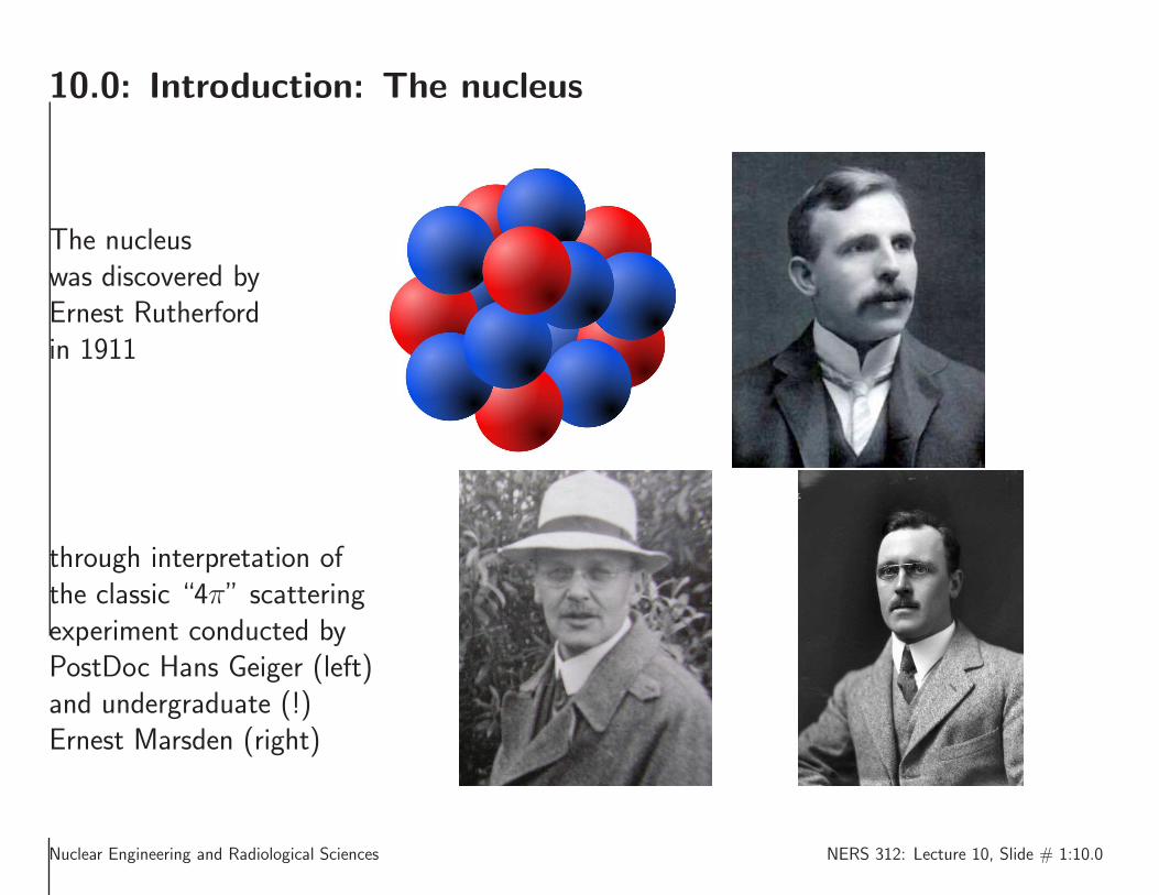
10.0: Introduction: The nucleus
The nucleuswas discovered byErnest Rutherfordin 1911
through interpretation ofthe classic “4π” scatteringexperiment conducted byPostDoc Hans Geiger (left)and undergraduate (!)Ernest Marsden (right)
Nuclear Engineering and Radiological Sciences NERS 312: Lecture 10, Slide # 1:10.0
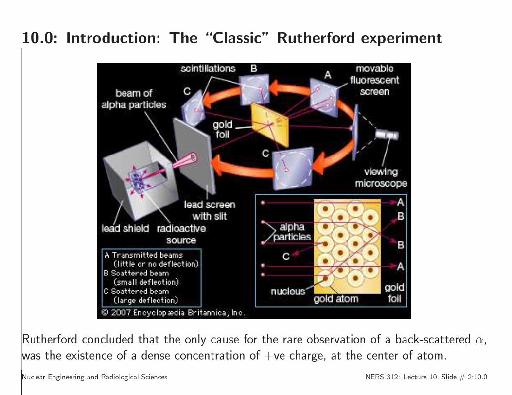
10.0: Introduction: The “Classic” Rutherford experiment
Rutherford concluded that the only cause for the rare observation of a back-scattered α,was the existence of a dense concentration of +ve charge, at the center of atom.
Nuclear Engineering and Radiological Sciences NERS 312: Lecture 10, Slide # 2:10.0

10.0: Introduction: The Nucleons
The nucleus is made up of protons and neutrons a.k.a. the “nucleons”.
Protons were proposed by William Prout in 1815and discovered by Rutherford in 1920
In 1920, Rutherford proposed existence of the neutronlater discovered by James Chadwick in 1932
Nuclear Engineering and Radiological Sciences NERS 312: Lecture 10, Slide # 3:10.0

10.0: Introduction: Characteristics of nucleons
Name mass charge lifetime magnetic moment(symbol) (MeV/c2) e (s) µN = e~/(2mp)
neutron (n) 939.565378(21) 0 881.5(1.5) -1.91304272(45)proton (p) 938.272046(21) 1 stable 2.792847356(23)
Charge Distribution:p all +ve charge peaks at about 0.45 fm, with an exponential die-off to ≈ 2 fmn has a +ve charge that peaks at 0.24 fm, followed by a -ve shell that peaks at 0.95 fmdies off exponentially, to about 2 fm Graphs on the next 2 pages
Properties Common to both nucleonsStructure Composite (quarks)
Radius ≈ 0.8 fmStatistics Fermi-Dirac (fermions)
Family Baryons (3 quarks)Intrinsic Spin 1
2~
Active forces Strong, electromagnetic, weak, gravity
Nuclear Engineering and Radiological Sciences NERS 312: Lecture 10, Slide # 4:10.0
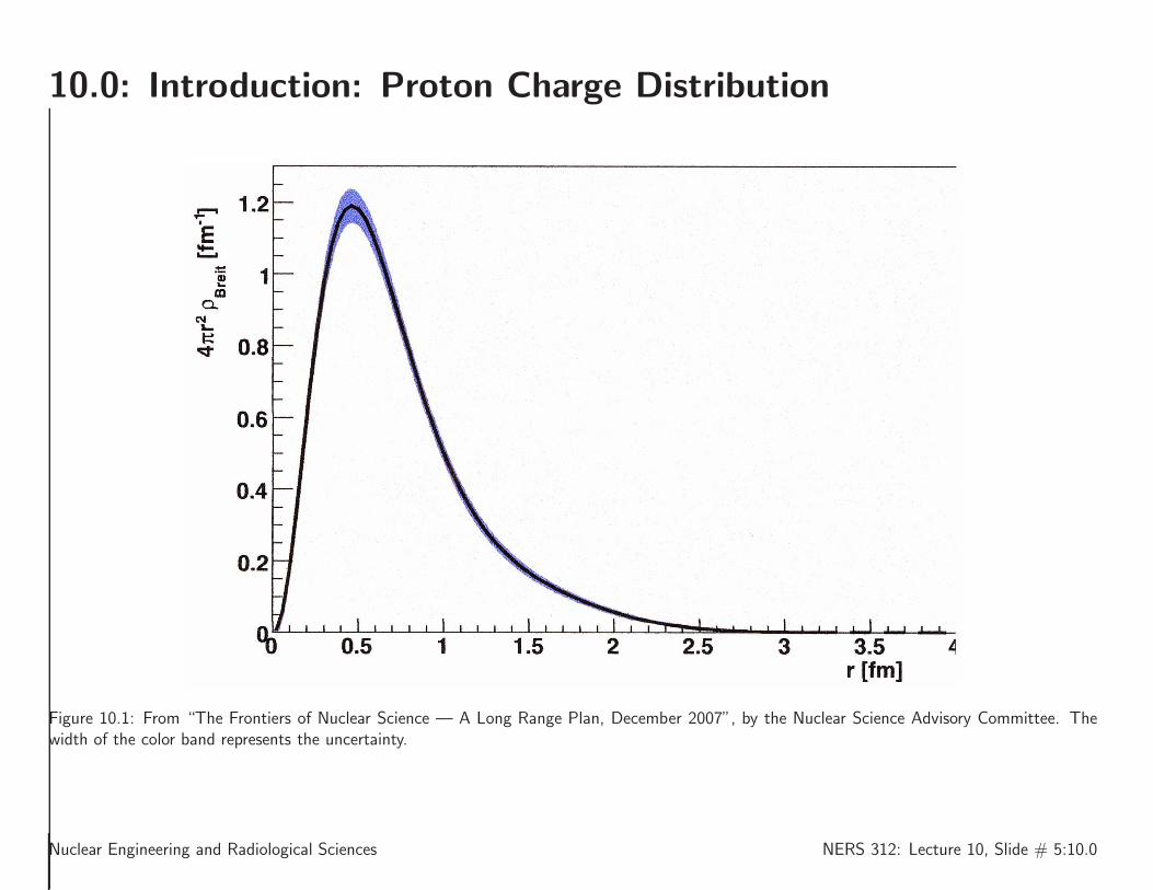
10.0: Introduction: Proton Charge Distribution
Figure 10.1: From “The Frontiers of Nuclear Science — A Long Range Plan, December 2007”, by the Nuclear Science Advisory Committee. Thewidth of the color band represents the uncertainty.
Nuclear Engineering and Radiological Sciences NERS 312: Lecture 10, Slide # 5:10.0
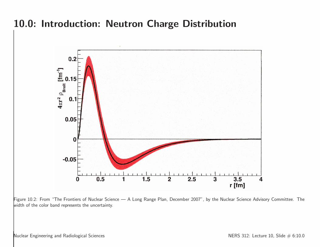
10.0: Introduction: Neutron Charge Distribution
Figure 10.2: From “The Frontiers of Nuclear Science — A Long Range Plan, December 2007”, by the Nuclear Science Advisory Committee. Thewidth of the color band represents the uncertainty.
Nuclear Engineering and Radiological Sciences NERS 312: Lecture 10, Slide # 6:10.0

10.0: Introduction: The nucleon-nucleon force
What binds two nucleons together?
• The nucleon force is a “derivative force”, generated by the underlying constituentparticles, much like an electrostatic dipole field is created by two nearby, equal charges,but of opposite sign.
• The n-n, n-p, and p-p nuclear forces are all almost identical.
• There is a strong short-range repulsive force, of the form:
V repnn (r) ≡ Arep
nn
rexp (−r/rrepnn ); where rrepnn ≈ 0.25 fm
• There is a strong medium-range attractive force, of the form:
V attnn (r) ≡ −A
attnn
rexp (−r/rattnn); where rattnn ≈ 0.36 fm &
Aattnn
Arepnn
≈ 0.67
• The combined force is:
Vnn(r) ≡Arepnn
rexp (−r/rrepnn )−
Aattnn
rexp (−r/rattnn)
Nuclear Engineering and Radiological Sciences NERS 312: Lecture 10, Slide # 7:10.0

10.0: Introduction: The nucleon-nucleon force
r(fm)0.2 0.4 0.6 0.8 1 1.2 1.4 1.6 1.8 2V
nn,rep(r)+Vnn,att(r)(arbitrary
units)
-10
-5
0
5
10
Total nucleon-nucleon force
attractive + repulsive
attractive
repulsive
Figure 10.3: The nucleon-nucleon potential, the sum of the repulsive (upper dashed line) and attractive (lower dash-dot line) nuclear potentials.
Nuclear Engineering and Radiological Sciences NERS 312: Lecture 10, Slide # 8:10.0

10.0: Introduction: The nucleon-nucleon force
The nucleon-nucleon force, key observations and conclusions
• The nuclear force bounds nucleons tightly, it is short-ranged. We can almost think ifit as a “contact” force. (Ping-pong balls covered in VaselineTM.)
• Nucleons are fermions, hence n’s and p’s tend to avoid each other.
• The nuclear part of the nucleon-nucleon force is central. (Ylml)!
• Protons are subject to a repulsive Coulomb force (also central).
• Since n’s and p’s have magnetic moments, they are both subject to magnet and motion(~v × ~B) forces, i.e. , spin-spin, and spin-orbit effects. These have enormous impactbecause the “magnets” are in close proximity.
Nuclear Engineering and Radiological Sciences NERS 312: Lecture 10, Slide # 9:10.0
10.0: Introduction: Some nomenclature
AZXN Isotope notationX Chemical symbol, e.g. Ca, PbA Atomic mass number (sum of n’s and p’s in the nucleus)Z Atomic number (or, proton number), the number of p’s in the nucleusN Neutron number, the number of n’s in the nucleus
Examples 32He1,
4020Ca20,
20882 Pb126
Variants 40Ca, Calcium-40, Ca-40
Note that, once X (which encodes Z) and A are given, the rest of the information isredundant, since A = Z +N . The full form is usually used only for emphasis.
isotope Same Z, different N e.g. 40Ca and 41CaMnemonic: From Greek isos (same) topos (place) (coined by F. Soddy 1913)
i.e. same place in the periodic table
isotone Different Z, same N , e.g. 13C and 12BMnemonic: isotoPe and isotoNe (coined by K. Guggenheimer 1934)
isobar Different Z, and N , but same A, e.g. 12C and 12BMnemonic: From Greek isos (same) baros (weight)
Nuclear Engineering and Radiological Sciences NERS 312: Lecture 10, Slide # 10:10.0
10.0: Introduction: Nucleus formation
How are nuclei formed?
• Because of the short-ranged nature of the nucleon-nucleon force, and its near extinctionat approximately 2 fm, nuclei are tightly bound, and each nucleon in the nuclear core(away from the surface), is bound only by its surrounding neighbors.
• Therefore, the nucleons in the core have their nuclear forces saturated, and it seemsto them, that they are in a constant, central (isotropic), nuclear potential. This is anestablished, experimentally-verified, fact.
• The nucleons near the surface, sometimes called the valence nucleons, are less bound,having fewer neighbors, than their “core” counterparts.
• Nucleons are quantum particles. Quantum particles in bound potentials have quantizedenergy levels.
• n’s and p’s are fermions, and hence subject to the Pauli Exclusion Principle, withintheir own group. Therefore, we may build up the nucleus, much as we did for theelectrons in the atomic shell (as in NERS 311), except that we have two distinctnucleons to account for.
Nuclear Engineering and Radiological Sciences NERS 312: Lecture 10, Slide # 11:10.0
10.0: Introduction: Nucleus formation
How are nuclei formed? (con’t)
• As a nucleus gains nucleons, Coulomb repulsion, a long-range force, is felt by all theprotons in the nucleus, that is, each proton feels the repulsion of all of the otherprotons in the nucleus. At some point, Coulomb repulsion overwhelms the nuclearbinding potential, and the nucleus can not be stable.
• Nuclei can offset this instability by increasing the number of n’s, compared to thenumber of p’s, thereby pushing the p’s to greater average radii. This strategy eventuallyfails for A > 208.
• The heaviest isotope with an equal number of n’s and p’s is calcium. The heavieststable isotope is lead, with A = 208.
• The strength of the nuclear force suggests that all nuclei are spherical in shape. (Thisis very nearly true. Exceptions will be discussed later in the course.) The radius of thenucleus will be discussed in the next section.
Nuclear Engineering and Radiological Sciences NERS 312: Lecture 10, Slide # 12:10.0

10.1: The nuclear radius
We have argued that the nucleus ought to be a spherical object.
Q: How to measure that? A: Bang things together and interpret!
Q: How?A: Bombard the nucleus with e−’s (electrons).
Measure their deflection, from the p’s in the nucleus.
Q: Can you get information about the radius of the nucleus?A: Yes! And as it turns out, that’s the best way to do it!
But, you should account for a few things ... a few very important things.
Nuclear Engineering and Radiological Sciences NERS 312: Lecture 10, Slide # 13:10.1

10.1: e− scattering to measure the radius of the nucleus
What projectile energy should I use?
Here we appeal to Quantum Mechanics:
The effective size of the wave associated with a relativistic electron is:
λ
2π=
~
pe=
~c
pec≈ ~c
Ee=
197 [MeV.fm]
Ee[MeV ]. RN ; RN ≡ radius of the nucleus[fm]
We now know that nuclear radii fall in the range 2–8 fm.
∴ Ee should be 10’s or even 100’s of MeV.
At much greater energy, about 2 GeV, one is able to “see” the quark structure inside anucleon!
How do I analyze the results of the scattering experiments?
Now, this is a long story ...
Nuclear Engineering and Radiological Sciences NERS 312: Lecture 10, Slide # 14:10.1

10.1: e− scattering analysis
It starts with consideration of a factor we’ll call the “scattering amplitude”, F , where
F (~ki, ~kf) = NF 〈ei~kf ·~x|V (~x)|ei~ki·~x〉 , (10.1)
where ...
ei~ki·~x ≡ the initial unscattered e− wavefunction
ei~kf ·~x ≡ the final scattered e− wavefunction~ki ≡ the initial e− wavenumber~kf ≡ the final e− wavenumberV (~x) ≡ the electrostatic Coulomb potential arising from the +ve charge distribution
in the nucleusNF ≡ a proportionality constant to be determined later
Nuclear Engineering and Radiological Sciences NERS 312: Lecture 10, Slide # 15:10.1

10.1: e− scattering analysis (con’t)
Evaluating ...
F (~ki, ~kf) = NF
∫
d~x e−i~kf ·~xV (~x)ei
~ki·~x
= NF
∫
d~x V (~x)ei(~ki−~kf )·~x
= NF
∫
d~x V (~x)ei~q·~x ,
where ~q ≡ ~ki − ~kf is called the momentum transfer.
It is the momentum taken (transferred) from ~ki to produce ~kf , since ~kf = ~ki − ~q .
We see that F is a function of the momentum transform alone:
F (~q) = NF
∫
d~x V (~x)ei~q·~x . (10.2)
We also see that scattering amplitude is proportional to the 3D Fourier Transform of thepotential. We are now, hopefully, in familiar mathematical territory!
Nuclear Engineering and Radiological Sciences NERS 312: Lecture 10, Slide # 16:10.1

10.1: e− scattering analysis (con’t)
We note, that the expression we started with, viz. F (~ki, ~kf) = NF 〈ei~kf ·~x|V (~x)|ei~ki·~x〉is completely general.
The 〈 〉 term is to be interpreted as follows:
V (~x) (whatever that happens to be) is an “action” that operates on the initial
wavefunction exp (i~ki · ~x).
The calculation implied by the 〈 〉, an integration over all space, measures the overlap of
the transformed (i.e. acted upon by V (~x)) initial wavefunction exp (i~ki · ~x), with the final
wavefunction exp (i~kf · ~x) .
How accurate is this “scattering factor”?
There are several approximations implied by our formulation, that we have not spoken of.
Can you suggest what they are?(It turns out that the approximations have little effect on our intended application.)
Nuclear Engineering and Radiological Sciences NERS 312: Lecture 10, Slide # 17:10.1

10.1: e− scattering analysis (con’t) (an aside on accuracy)
In this application...
1. V (~x) is treated as a classical, continuous charge distribution. In fact, the operatoris made up of the quantum mechanical E&M operator over the composite protonwavefunction.
2. The proton charge density is not continuous, nor is it static.
3. The initial and final wavefunctions are not distorted by the potential. This is called theFirst Born Approximation. It happens to work for this application because the E&Mforces are relatively weak.
Returning to our analysis ...
Nuclear Engineering and Radiological Sciences NERS 312: Lecture 10, Slide # 18:10.1

10.1: e− scattering analysis (con’t)
The scattering potential takes the form:
V (~x) = −Ze2
4πǫ0
∫
d~x′ρp(~x
′)
|~x− ~x′| , (10.3)
ρp(~x′) ≡ the “number” density of protons in the nucleus, normalized so that:
∫
d~x′ ρp(~x′) ≡ 1 . (10.4)
The potential at ~x arises from the electrostatic attraction of the elemental charges in d~x,integrated over the nucleus.Putting it all together:
F (~q) = NF
(
−Ze2
4πǫ0
)∫
d~x
∫
d~x′ρp(~x
′)
|~x− ~x′|ei~q·~x . (10.5)
We choose the constant of proportionality in F (~q), to require that F (0) ≡ 1. Themotivation for this choice is that, when ~q = 0, the charge distribution is known to have noeffect on the projectile. If a potential has no effect on the projectile, then we can rewrite(10.5) as
F (0) ≡ 1 = NF
(
−Ze2
4πǫ0
)∫
d~x
∫
d~x′ρp(~x
′)
|~x− ~x′| , or... (10.6)
Nuclear Engineering and Radiological Sciences NERS 312: Lecture 10, Slide # 19:10.1

10.1: e− scattering analysis (con’t)
NF =
[(
−Ze2
4πǫ0
)∫
d~x
∫
d~x′ρp(~x
′)
|~x− ~x′|
]−1
,
and
F (~q) =
[∫
d~x
∫
d~x′ρp(~x
′)
|~x− ~x′|ei~q·~x
]/[∫
d~x
∫
d~x′ρp(~x
′)
|~x− ~x′|
]
Remarkably, we can collapse the expression above significantly.
The details of this calculation will be left to enthusiastic students to discover for them-selves. The final result is:
F (~q) =
∫
d~x ρp(~x)ei~q·~x , (10.7)
and the “scattering amplitude” has been shown to be the 3D Fourier transform of thecharge distribution.
We shall soon see, that√
|F (~q)|2 is a function that can be explicitly measured inexperiments.
First, let’s work out some simple examples of F (~q).
Nuclear Engineering and Radiological Sciences NERS 312: Lecture 10, Slide # 20:10.1

10.1.1: F (~q) for spherical charge distributions
For spherical charge distributions (the usual case), ρp(~x) = ρp(r), (10.7) can be furtherreduced. We start with:
F (~q) =
∫
d~x ρp(~x)ei~q·~x
Now, we convert (x, y, z) −→ (r, θ, φ) and align ~q −→ qz.Since the charge distribution is spherically symmetric, we can choose any axis to align ~qwith, and the z-axis is the most convenient.
F (q) =
∫ 2π
0
dφ
∫ ∞
0
r2dr ρp(r)
∫ π
0
sin θ dθ eiqr cos θ [note F (~q) −→ F (q)] (10.8)
= 2π
∫ ∞
0
r2dr ρp(r)
∫ π
0
sin θ dθ eiqr cos θ [did the integral over φ]
= 2π
∫ ∞
0
r2dr ρp(r)
∫ 1
−1
dµ eiqrµ [change of variable µ = cos θ]
= 2π
∫ ∞
0
rdr ρp(r)
(
2
q
)
sin qr [did the integral over µ]
=4π
q
∫ ∞
0
rdr ρp(r) sin qr [in final form] (10.9)
Nuclear Engineering and Radiological Sciences NERS 312: Lecture 10, Slide # 21:10.1
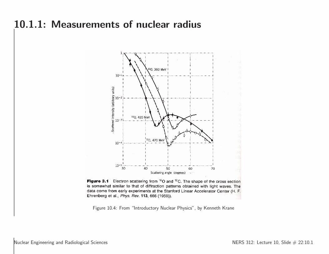
10.1.1: Measurements of nuclear radius
Figure 10.4: From “Introductory Nuclear Physics”, by Kenneth Krane
Nuclear Engineering and Radiological Sciences NERS 312: Lecture 10, Slide # 22:10.1

10.1.1: Measurements of nuclear radius
Figure 10.5: From “Introductory Nuclear Physics”, by Kenneth Krane
Nuclear Engineering and Radiological Sciences NERS 312: Lecture 10, Slide # 23:10.1
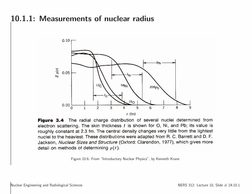
10.1.1: Measurements of nuclear radius
Figure 10.6: From “Introductory Nuclear Physics”, by Kenneth Krane
Nuclear Engineering and Radiological Sciences NERS 312: Lecture 10, Slide # 24:10.1
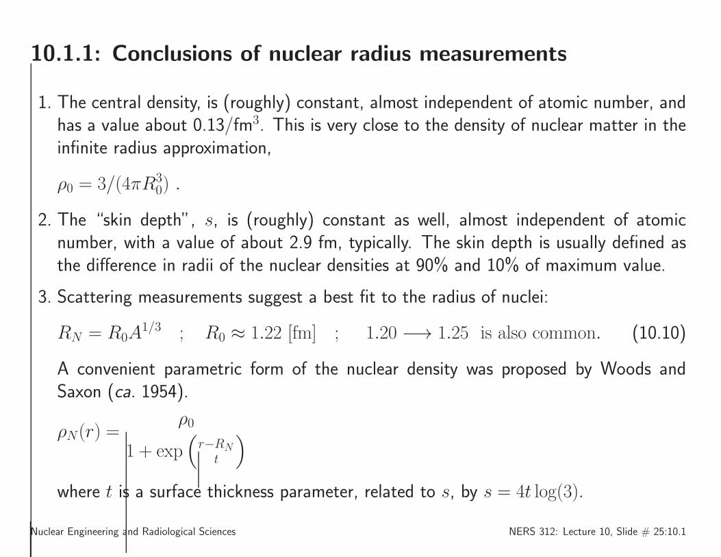
10.1.1: Conclusions of nuclear radius measurements
1. The central density, is (roughly) constant, almost independent of atomic number, andhas a value about 0.13/fm3. This is very close to the density of nuclear matter in theinfinite radius approximation,
ρ0 = 3/(4πR30) .
2. The “skin depth”, s, is (roughly) constant as well, almost independent of atomicnumber, with a value of about 2.9 fm, typically. The skin depth is usually defined asthe difference in radii of the nuclear densities at 90% and 10% of maximum value.
3. Scattering measurements suggest a best fit to the radius of nuclei:
RN = R0A1/3 ; R0 ≈ 1.22 [fm] ; 1.20 −→ 1.25 is also common. (10.10)
A convenient parametric form of the nuclear density was proposed by Woods andSaxon (ca. 1954).
ρN(r) =ρ0
1 + exp(
r−RNt
)
where t is a surface thickness parameter, related to s, by s = 4t log(3).
Nuclear Engineering and Radiological Sciences NERS 312: Lecture 10, Slide # 25:10.1

10.1.1: Conclusions of nuclear radius measurements (con’t)
r(fm)0 2 4 6 8 10 12
ρN(r)(fm
−3)
0
0.02
0.04
0.06
0.08
0.1
0.12
0.14Nucleon number density of nucleus A = 208
Figure 10.7: The Woods-Saxon model of the nucleon number density. In this figure, A = 208, R0 = 1.22 (fm), and t = 0.65 (fm). The skin depthis shown, delimited by vertical dotted lines.
Nuclear Engineering and Radiological Sciences NERS 312: Lecture 10, Slide # 26:10.1
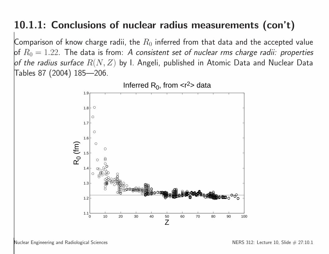
10.1.1: Conclusions of nuclear radius measurements (con’t)
Comparison of know charge radii, the R0 inferred from that data and the accepted valueof R0 = 1.22. The data is from: A consistent set of nuclear rms charge radii: propertiesof the radius surface R(N,Z) by I. Angeli, published in Atomic Data and Nuclear DataTables 87 (2004) 185—206.
0 10 20 30 40 50 60 70 80 90 1001.1
1.2
1.3
1.4
1.5
1.6
1.7
1.8
1.9
Z
R0
(fm
)Inferred R0, from <r2> data
Nuclear Engineering and Radiological Sciences NERS 312: Lecture 10, Slide # 27:10.1

10.1.1: Conclusions of nuclear radius measurements (con’t)
190 195 200 205 210 215
A
1.198
1.2
1.202
1.204
1.206
1.208
1.21
1.212
1.214
1.216
1.218R
0 (
fm)
Inferred R0
for known isotopes of Pb
Nuclear Engineering and Radiological Sciences NERS 312: Lecture 10, Slide # 28:10.1

10.1.1: Conclusions of nuclear radius measurements (con’t)
80 81 82 83 84 85 86 87 88 891.196
1.198
1.2
1.202
1.204
1.206
1.208
1.21
Z
R0
(fm
)Inferred R
0 from A = 208
Nuclear Engineering and Radiological Sciences NERS 312: Lecture 10, Slide # 29:10.1
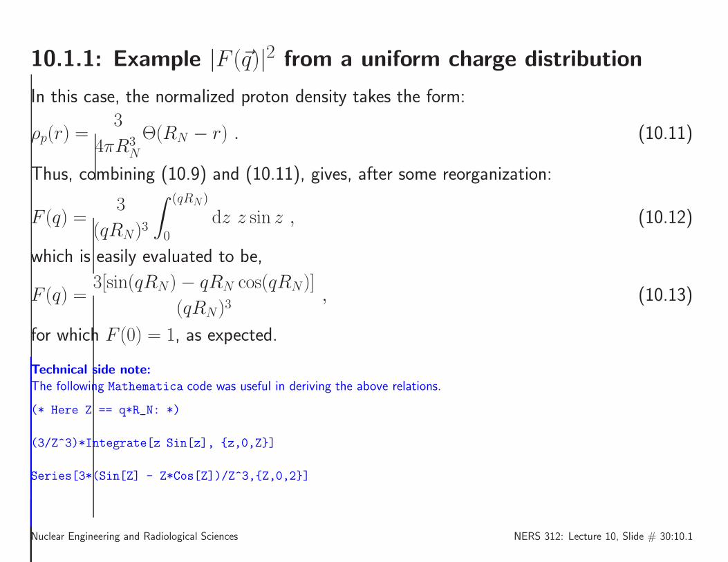
10.1.1: Example |F (~q)|2 from a uniform charge distribution
In this case, the normalized proton density takes the form:
ρp(r) =3
4πR3N
Θ(RN − r) . (10.11)
Thus, combining (10.9) and (10.11), gives, after some reorganization:
F (q) =3
(qRN)3
∫ (qRN )
0
dz z sin z , (10.12)
which is easily evaluated to be,
F (q) =3[sin(qRN)− qRN cos(qRN)]
(qRN)3, (10.13)
for which F (0) = 1, as expected.
Technical side note:
The following Mathematica code was useful in deriving the above relations.
(* Here Z == q*R_N: *)
(3/Z^3)*Integrate[z Sin[z], z,0,Z]
Series[3*(Sin[Z] - Z*Cos[Z])/Z^3,Z,0,2]
Nuclear Engineering and Radiological Sciences NERS 312: Lecture 10, Slide # 30:10.1

10.1.1: ...Example |F (~q)|2 from a uniform charge distribution...
Note the minima when tan(qRN) = qRN . Measurements do not have such deep minima,because: 1) the nuclear edge is blurred, not sharp, 2) the projectiles are polyenergetic,3) the detectors have imperfect resolution.
0 2 4 6 8 10 12 14 16 18 20−6
−5
−4
−3
−2
−1
0
q*RN
log 1
0|f(
q*R
N)|
2
Figure 10.8: Graphical output corresponding to (10.13).
Nuclear Engineering and Radiological Sciences NERS 312: Lecture 10, Slide # 31:10.1

10.1.1: ...Example |F (~q)|2 from a uniform charge distribution...
Technical side note:The following Matlab code was useful in producing the above graph.
N = 1000; fMin = 1e-6; zMax = 20; % Graph data
z = linspace(0,zMax,N); f = 3*(sin(z) - z.*cos(z))./z.^3;
f(1) = 1; % Overcome the singularity at 0
f2 = f.*f;
for i = 1:N
f2(i) = max(fMin,f2(i));
end
plot(z,log10(f2),’-k’)
xlabel(’\fontsize20q*R_N’)
ylabel(’\fontsize20log_10|f(q*R_N)|^2’)
Nuclear Engineering and Radiological Sciences NERS 312: Lecture 10, Slide # 32:10.1
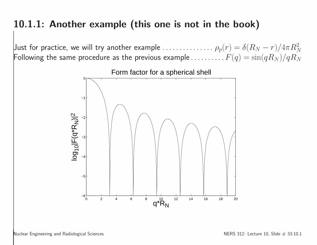
10.1.1: Another example (this one is not in the book)
Just for practice, we will try another example . . . . . . . . . . . . . . . ρp(r) = δ(RN − r)/4πR2N
Following the same procedure as the previous example . . . . . . . . . .F (q) = sin(qRN)/qRN
0 2 4 6 8 10 12 14 16 18 20−6
−5
−4
−3
−2
−1
0
q*RN
log 1
0|F
(q*R
N)|
2Form factor for a spherical shell
Nuclear Engineering and Radiological Sciences NERS 312: Lecture 10, Slide # 33:10.1

10.1.2: Finally ... how to get F (q) from measurements
Technical side note: The mathematical details can be found in the supplemental notes.
The supplementary notes obtain the following, very significant result, that a full quantummechanical derivation of the cross section of e−N scattering obtains the following result:
dσeNdΩ
=dσRutheN
dΩ|F (q)|2 , (10.14)
where dσRutheN /dΩ is the classical Rutherford cross section discussed in NERS311, and|F (q)|2 is the scattering amplitude that we have been discussing.
Hence, we have a direct experimental determination of the form factor, as a ratio ofthe measurement data (the measured cross section), to the theoretical function (theRutherford cross section):
|F (q)|2 =(
dσmeaseN
dΩ
)
/
(
dσRutheN
dΩ
)
. (10.15)
Nuclear Engineering and Radiological Sciences NERS 312: Lecture 10, Slide # 34:10.1

10.1.2: The quantum mechanical Rutherford cross section
All that remains is to take the square root, and invert the Fourier Transform, to get ρ(r).This is always done via a relatively simple numerical process.
Although the form factor |F (q)|2 is given in terms of q, we may cast it into more recog-nizable kinematic quantities as follows. Recall,
q =√
q2 =
√
|~ki − ~kf |2 =√
2k2(1− cos θ) , (10.16)
the final step above being obtained since this is an elastic scattering process, where
k = |~ki| = |~kf | and ~ki · ~kf = k2 cos θ.
Nuclear Engineering and Radiological Sciences NERS 312: Lecture 10, Slide # 35:10.1

10.1.3: Nuclear size from spectroscopy measurements
An ideal probe of the effect of a finite-sized nucleus, would be a 1s atomic state.
The 1s state has the most probability density in the vicinity of the nucleus.
The shift of energy (from 1st-order perturbation theory), of the 1s can be estimated asfollows:
∆E1s = 〈ψ1s|V(r)− V.(r)|ψ1s〉 , (10.17)
where the ψ1s is the 1s wavefunction for the point-like nucleus, V(r) is the Coulombpotential for the finite nucleus, and V.(r) is the point-like Coulomb potential.
Nuclear Engineering and Radiological Sciences NERS 312: Lecture 10, Slide # 36:10.1

10.1.3: Nuclear size from spectroscopy measurements (con’t)
For a uniform sphere of charge, we know from Classical Electrostatics, that V(r) = V.(r)for r ≥ RN .
V.(0 ≤ r <∞) = − Ze2
4πǫ0r
V(r ≤ RN) = − Ze2
4πǫ0RN
[
3
2− 1
2
(
r
RN
)2]
V(r ≥ RN) = V.(r ≥ RN) (10.18)
or
V(r)− V.(r) =Ze2
4πǫ0RN
[
RN
r− 3
2+1
2
(
r
RN
)2]
θ(RN − r)
We evaluate this by combining the above with ∆E1s = 〈ψ1s|V(r)−V.(r)|ψ1s〉 and usingthe hydrogenic wavefunctions given in NERS311 and also in Krane II (Tables 2.2 and 2.5)
ψ1s,(n,l,ml)=(1,0,0) =
Rn=1,l=0(r) [
Yl=0,ml=0(θ, φ)]
=
2
(
Z
a0
)3/2
e−Zr/a0
[
1
4π
]1/2
Nuclear Engineering and Radiological Sciences NERS 312: Lecture 10, Slide # 37:10.1

10.1.3: Nuclear size from spectroscopy measurements (con’t)
and obtain:
∆E1s = 〈ψ1s|V(r)− V.(r)|ψ1s〉∫ 2π
0
dφ
∫ π
0
dθ sin θ
∫ ∞
0
dr r2|ψ1s(~x)|2[V(r)− V.(r)]
e2
4πǫ0
4Z4
a30
1
RN
∫ RN
0
drr2e−2Zr/a0
[
RN
r− 3
2+
1
2
(
r
RN
)2]
, (10.19)
where a0 = 5.2917721092(17)× 10−11 m, i.e., the Bohr radius.
Nuclear Engineering and Radiological Sciences NERS 312: Lecture 10, Slide # 38:10.1

10.1.3: Nuclear size from spectroscopy measurements (con’t)
In unitless quantities, we may rewrite the above as:
∆E1s = Z2α2(mec2)
(
2ZRN
a0
)2 ∫ 1
0
dze−(2ZRN/a0)z
[
z − 3
2z2 +
z4
2
]
. (10.20)
α = e2
4πǫ0~c= 1
137.035999074(44)(fine-structure constant, unitless).
Across all the elements, the dimensionless parameter (2ZRN/a0) spans the range2×10−5 −→≈ 10−2. Hence, the contribution to the exponential, in the integral, is incon-sequential. (You should not make this approximation for muonic atoms [next section].)The remaining integral is a pure number and evaluates to 1/10. Thus, we may write:
∆E1s ≈1
10Z2α2(mec
2)
(
2ZRN
a0
)2
. (10.21)
This correction is about 1 eV for Z = 100 and much smaller for lighter nuclei.
This is a very small difference!
Nuclear Engineering and Radiological Sciences NERS 312: Lecture 10, Slide # 39:10.1

10.1.3: Nuclear size from spectroscopy measurements (con’t)
Not only is this shift in energy small, it measures the shift in energy by introducing arealistic charge distribution, and comparing the bound state energy with the bound-stateenergy arising from a point nucleus.
Point nuclei, do not exist in nature, so, we still have work to do!
We don’t have anything to compare with experiment yet.
So ...
Nuclear Engineering and Radiological Sciences NERS 312: Lecture 10, Slide # 40:10.1

10.1.3: Nuclear size from spectroscopy measurements (con’t)
Nuclear size determination from an isotope shift measurement
Let us imagine how we are to determine the nuclear size, by measuring the energy of thephoton that is given off, from a 2p→ 1s transition.
The Schrodinger equation predicts that the energy of the photon will be given by:
(E2p→1s) = (E2p→1s). + 〈ψ2p|V(r)− V.(r)|ψ2p〉 − 〈ψ1s|V(r)− V.(r)|ψ1s〉 , (10.22)
or,
(∆E2p→1s) = 〈ψ2p|V(r)− V.(r)|ψ2p〉 − 〈ψ1s|V(r)− V.(r)|ψ1s〉 , (10.23)
expressing the change in the energy of the photon, due to the effect of finite nuclear size.
The latter term, 〈ψ1s|V(r)−V.(r)|ψ1s〉, has been calculated in (10.21). We now considerthe former term, 〈ψ2p|V(r)− V.(r)|ψ2p〉...
Nuclear Engineering and Radiological Sciences NERS 312: Lecture 10, Slide # 41:10.1

10.1.3: Nuclear size from spectroscopy measurements (con’t)
0 0.5 1 1.5 2 2.5 3 3.5 4 4.5 50
0.1
0.2
0.3
0.4
0.5
0.6
0.7
0.8
0.9
1
Zr/a0
R/R
max
(0)
R1s/R1s,max
R2p/R2p,max
10*RN
(Pb)
Figure 10.9: Overlap of 1s and 2p electronic orbitals with the nuclear radius. The nuclear radius depicted is for A = 208 and has been scaled upwardby 10 for display purposes.
Figure 10.9 shows the 1s and 2p hydrogenic radial probabilities for the 1s and 2p states,each divided by their respective maxima. The vertical line near the origin is the 10× theradius of an A = 208, Z = 82 nucleus.
Nuclear Engineering and Radiological Sciences NERS 312: Lecture 10, Slide # 42:10.1

10.1.3: Nuclear size from spectroscopy measurements (con’t)
The overlap of the 2p state with the nucleus is ≪ than that of the 1s state. Hence,〈ψ2p|V(r)− V.(r)|ψ2p〉 ≈ 0. Therefore, that the transition photon’s energy is:
∆E2p→1s ≈ −〈ψ1s|V(r)− V.(r)|ψ1s〉 ≈ − 1
10Z2α2(mec
2)A2/3
(
2ZR0
a0
)2
. (10.24)
Still do not have anything we can measure!We can not measure a photon’s energy from a point nucleus!Instead, measure the transition energy for two isotopes of the same element, A and A′.The point nucleus drops out of the equation (and the measurement):
∆E2p→1s(A) − ∆E2p→1s(A′) =
= −〈1s|V(r)− V.(r)|1s〉|A + 〈1s|V(r)− V.(r)|1s〉|A′
= 〈1s|V(r)|1s〉|A′ − 〈1s|V(r)|1s〉|A−〈1s|V.(r)|1s〉|A′ + 〈1s|V.(r)|1s〉|A= 〈1s|V(r)|1s〉|A′ − 〈1s|V(r)|1s〉|A 〈1s|V.(r)|1s〉A − [〈1s|V.(r)|1s〉A′ = 0
=1
10Z2α2(mec
2)
(
2ZR0
a0
)2
(A′2/3 − A2/3) . (10.25)
Nuclear Engineering and Radiological Sciences NERS 312: Lecture 10, Slide # 43:10.1
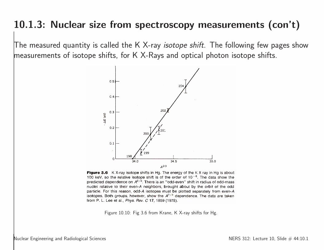
10.1.3: Nuclear size from spectroscopy measurements (con’t)
The measured quantity is called the K X-ray isotope shift. The following few pages showmeasurements of isotope shifts, for K X-Rays and optical photon isotope shifts.
Figure 10.10: Fig 3.6 from Krane, K X-ray shifts for Hg.
Nuclear Engineering and Radiological Sciences NERS 312: Lecture 10, Slide # 44:10.1

10.1.3: Nuclear size from spectroscopy measurements (con’t)
Figure 10.11: Fig 3.7 from Krane, optical shifts for Hg.
Nuclear Engineering and Radiological Sciences NERS 312: Lecture 10, Slide # 45:10.1

10.1.3: Nuclear size from spectroscopy measurements (con’t)
A better probe of nuclear shape can be done by forming muonic atoms, formed from muons(usually from cosmic rays), that replace an inner K-shell electron, and has significantoverlap of its wavefunction with the nucleus.
Figure 10.12: Fig 3.8 from Krane, K X-ray shifts for muonic Fe.
Nuclear Engineering and Radiological Sciences NERS 312: Lecture 10, Slide # 46:10.1
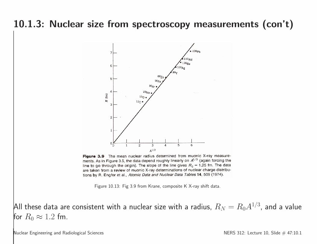
10.1.3: Nuclear size from spectroscopy measurements (con’t)
Figure 10.13: Fig 3.9 from Krane, composite K X-ray shift data.
All these data are consistent with a nuclear size with a radius, RN = R0A1/3, and a value
for R0 ≈ 1.2 fm.
Nuclear Engineering and Radiological Sciences NERS 312: Lecture 10, Slide # 47:10.1

10.1.3: Charge radius from Coulomb energy in mirror nuclei...
Charge radius from Coulomb energy in mirror nuclei
A mirror-pair of nuclei are two nuclei that have the same atomic mass, but the numberof protons in one, is the number of neutrons in the other, and the number of protonsand neutrons in one of the nuclei differs by only 1. So, if Z is the atomic number of thehigher atomic number mirror nucleus, it has Z − 1 neutrons. Its mirror pair has Z − 1protons and Z neutrons. The atomic mass of both is 2Z − 1. Examples of mirror pairsare: 3H/3He, and 39Ca/39K.
These mirror-pairs are excellent laboratories for investigating nuclear radius since thenuclear component of the binding energy of these nuclei ought to be the same, if thestrong force does not distinguish between nucleons. The only remaining difference is theCoulomb self-energy, and that is related to the radius.
Nuclear Engineering and Radiological Sciences NERS 312: Lecture 10, Slide # 48:10.1

10.1.3: ...Charge radius from Coulomb energy in mirror nuclei...
For a charge distribution with Z protons, the Coulomb self-energy is:
EC =1
2
Z2e2
4πǫ0
∫
d~x1ρp(~x1)
∫
d~x2ρp(~x2)1
|~x1 − ~x2|. (10.26)
The factor of 1/2 in front of (10.26) accounts for the double counting of repulsion thattakes place when one integrates over the nucleus twice, as implied in (10.26).For a uniform, spherical charge distribution of the form,
ρp(~x) =3
4πR3N
Θ(RN − r) . (10.27)
As derived on the next pages:
EC =3
5
Z2e2
4πǫ0RN. (10.28)
Nuclear Engineering and Radiological Sciences NERS 312: Lecture 10, Slide # 49:10.1

10.1.3: ...Charge radius from Coulomb energy in mirror nuclei...
For a uniform, spherical charge distribution, given by (10.27):
EC =1
2
Z2e2
4πǫ0
(
3
4πR3N
)2 ∫
|~x1|≤RNd~x1
∫
|~x2|≤RNd~x2
1
|~x1 − ~x2|
=1
2
Z2e2
4πǫ0RN
(
3
4π
)2 ∫
|~u1|≤1
d~u1
∫
|~u2|≤1
d~u21
|~u1 − ~u2|[~x→ r~u for both integrals]
=1
2
Z2e2
4πǫ0RNI , (10.29)
where
I =
(
3
4π
)2 ∫
|~u1|≤1
d~u1
∫
|~u2|≤1
d~u21
|~u1 − ~u2|. (10.30)
From (10.30), one sees that I has the interpretation as a pure number representing theaverage of |~u1 − ~u2|−1, for two vectors, ~u1 and ~u2, integrated uniformly over the interiorof a unit sphere. So, now it just remains, to calculate I . We’ll work this out explicitlybecause the calculation is quite delicate.
Nuclear Engineering and Radiological Sciences NERS 312: Lecture 10, Slide # 50:10.1
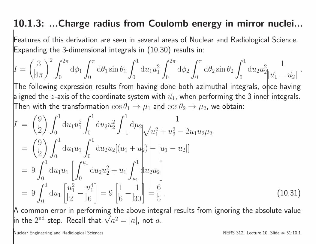
10.1.3: ...Charge radius from Coulomb energy in mirror nuclei...
Features of this derivation are seen in several areas of Nuclear and Radiological Science.Expanding the 3-dimensional integrals in (10.30) results in:
I =
(
3
4π
)2 ∫ 2π
0
dφ1
∫ π
0
dθ1 sin θ1
∫ 1
0
du1u21
∫ 2π
0
dφ2
∫ π
0
dθ2 sin θ2
∫ 1
0
du2u22
1
|~u1 − ~u2|.
The following expression results from having done both azimuthal integrals, once havingaligned the z-axis of the coordinate system with ~u1, when performing the 3 inner integrals.Then with the transformation cos θ1 → µ1 and cos θ2 → µ2, we obtain:
I =
(
9
2
)∫ 1
0
du1u21
∫ 1
0
du2u22
∫ 1
−1
dµ21
√
u21 + u22 − 2u1u2µ2
=
(
9
2
)∫ 1
0
du1u1
∫ 1
0
du2u2[(u1 + u2)− |u1 − u2|]
= 9
∫ 1
0
du1u1
[∫ u1
0
du2u22 + u1
∫ 1
u1
du2u2
]
= 9
∫ 1
0
du1
[
u212− u41
6
]
= 9
[
1
6− 1
30
]
=6
5. (10.31)
A common error in performing the above integral results from ignoring the absolute valuein the 2nd step. Recall that
√a2 = |a|, not a.
Nuclear Engineering and Radiological Sciences NERS 312: Lecture 10, Slide # 51:10.1

10.1.3: ...Charge radius from Coulomb energy in mirror nuclei...
Finally, combining (10.29) and (10.31) gives us the final result expressed in (10.28).The Coulomb energy differences are measured through β-decay endpoint energies (moreon this later in the course), which yield very good information on the nuclear radius. Thedifference in Coulomb energies is given by:
∆EC =3
5
e2
4πǫ0RN[Z2 − (Z − 1)2]
=3
5
e2
4πǫ0RN(2Z − 1)
=3
5
e2
4πǫ0R0A2/3 , (10.32)
where, in the last step, we let RN = R0A1/3.
Recall, A = 2Z − 1 for mirror nuclei.
Nuclear Engineering and Radiological Sciences NERS 312: Lecture 10, Slide # 52:10.1
10.1.3: ...Charge radius from Coulomb energy in mirror nuclei...
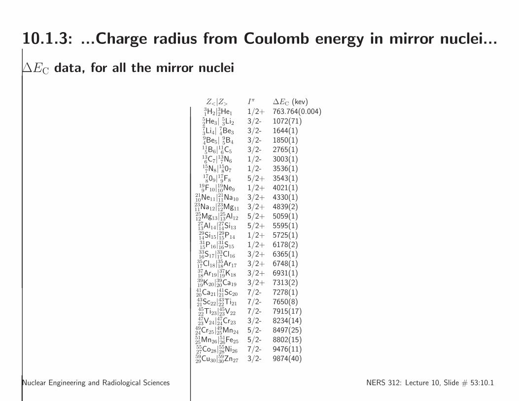
∆EC data, for all the mirror nuclei
Z<|Z> Iπ ∆EC (kev)3
1H2|32He1 1/2+ 763.764(0.004)5
2He3| 5
3Li2 3/2- 1072(71)
73Li4| 7
4Be3 3/2- 1644(1)9
4Be5| 9
5B4 3/2- 1850(1)
11
5B6|116C5 3/2- 2765(1)
136C7|137N6 1/2- 3003(1)15
7N8|15807 1/2- 3536(1)
17
809|179F8 5/2+ 3543(1)
19
9F10|1910Ne9 1/2+ 4021(1)
2110Ne11|2111Na10 3/2+ 4330(1)23
11Na12|2312Mg11 3/2+ 4839(2)
25
12Mg13|2513Al12 5/2+ 5059(1)
2713Al14|2714Si13 5/2+ 5595(1)29
14Si15|2915P14 1/2+ 5725(1)
31
15P16|3116S15 1/2+ 6178(2)33
16S17|3317Cl16 3/2+ 6365(1)
35
17Cl18|3518Ar17 3/2+ 6748(1)
3718Ar19|3719K18 3/2+ 6931(1)39
19K20|3920Ca19 3/2+ 7313(2)
4120Ca21|4121Sc20 7/2- 7278(1)43
21Sc22|4322Ti21 7/2- 7650(8)
45
22Ti23|4523V22 7/2- 7915(17)47
23V24|4724Cr23 3/2- 8234(14)
49
24Cr25|4925Mn24 5/2- 8497(25)
5125Mn26|5126Fe25 5/2- 8802(15)55
27Co28|5528Ni26 7/2- 9476(11)
59
29Cu30|5930Zn27 3/2- 9874(40)
Nuclear Engineering and Radiological Sciences NERS 312: Lecture 10, Slide # 53:10.1
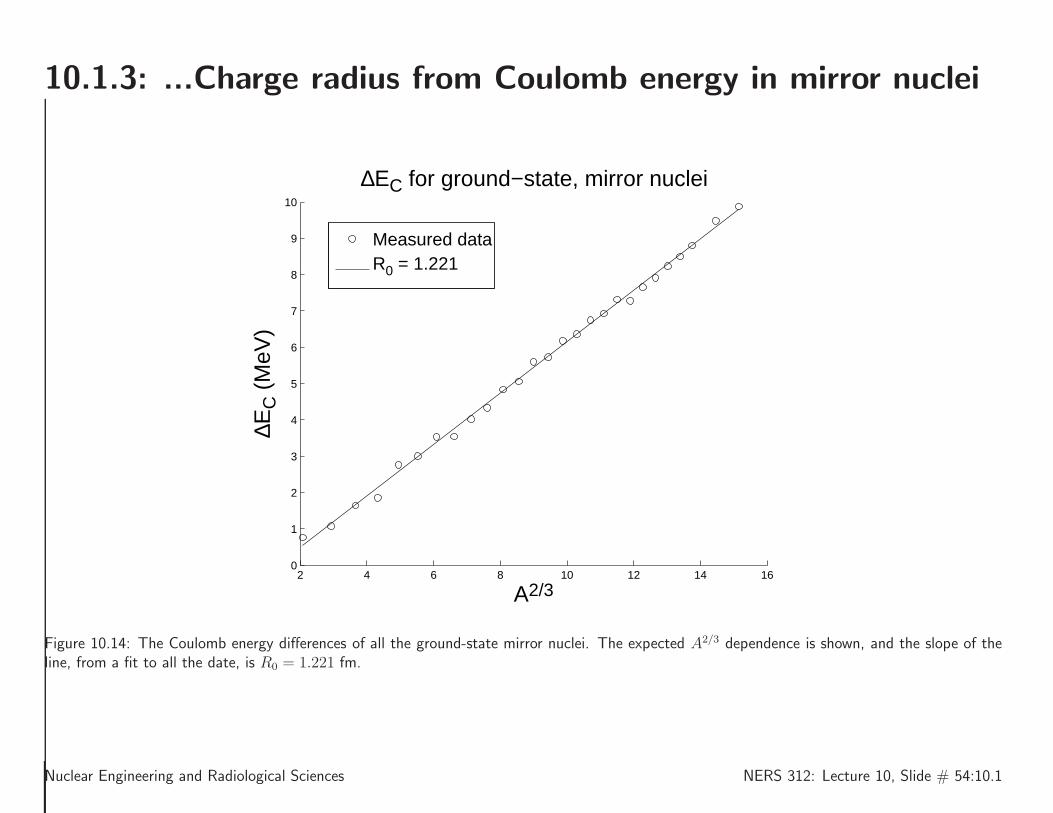
10.1.3: ...Charge radius from Coulomb energy in mirror nuclei
2 4 6 8 10 12 14 160
1
2
3
4
5
6
7
8
9
10
A2/3
∆EC
(M
eV)
∆EC for ground−state, mirror nuclei
Measured dataR0 = 1.221
Figure 10.14: The Coulomb energy differences of all the ground-state mirror nuclei. The expected A2/3 dependence is shown, and the slope of theline, from a fit to all the date, is R0 = 1.221 fm.
Nuclear Engineering and Radiological Sciences NERS 312: Lecture 10, Slide # 54:10.1

10.1.3: ...Charge radius from Coulomb energy in mirror nuclei
0 2 4 6 8 10 12 14 160
1
2
3
4
5
6
7
8
9
10
A2/3
∆EC
(M
eV)
∆EC for ground−state, mirror nuclei
Measured dataR0 = 1.10 for A = [5−15]
R0 = 1.14 for A = [17−39]
R0 = 1.07 for A = [41−59]
The Coulomb energy differences of all the ground-state mirror nuclei, with separate fitswithin shell.
Nuclear Engineering and Radiological Sciences NERS 312: Lecture 10, Slide # 55:10.1
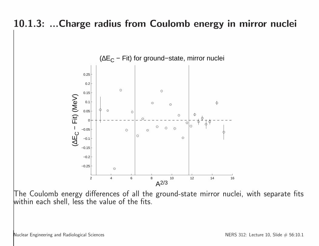
10.1.3: ...Charge radius from Coulomb energy in mirror nuclei
2 4 6 8 10 12 14 16
−0.25
−0.2
−0.15
−0.1
−0.05
0
0.05
0.1
0.15
0.2
0.25
A2/3
(∆E
C −
Fit)
(M
eV)
(∆EC − Fit) for ground−state, mirror nuclei
The Coulomb energy differences of all the ground-state mirror nuclei, with separate fitswithin each shell, less the value of the fits.
Nuclear Engineering and Radiological Sciences NERS 312: Lecture 10, Slide # 56:10.1
10.2: Mass and Abundance of Nuclei
Note to students: Read 3.2 in Krane on your own. You are responsible for this material,but it will not be covered in class.
Nuclear Engineering and Radiological Sciences NERS 312: Lecture 10, Slide # 57:10.2

10.3: Nuclear binding energy
Atomic and Nuclear rest mass energies
The rest mass energy of a neutral atom, mAc2 (often called m(AX)c2) and the rest mass
energy of its nucleus, mNc2, are related by:
mAc2 = m
Nc2 + [Zmec
2 −Be(Z,A)] , (10.33)
where Be(Z,A) is the electronic binding, the sum of the binding energies of all theelectrons in the atomic cloud, i.e.
Be(Z,A) =Z∑
i=1
Bei ,
where Bei is the electronic binding energy of the i’th atomic electron.
Be(Z,A) can be as large as 1 MeV in the heavier atoms!
However, Be(Z,A) is swamped by factors of 105–106 by mNc2 ≈ A× 1000 MeV.
Hence, mAc2 ≈ m
Nc2+Zmec
2 , is used for simplicity, particularly when mass differencesare discussed, as the electronic binding component largely cancels out.
Nuclear Engineering and Radiological Sciences NERS 312: Lecture 10, Slide # 58:10.3

10.3: ...Nuclear binding energy (con’t)...
One may estimate the total electronic binding as done in the following example.
Technical aside: Estimating the electronic binding in Pb:
Lead has the following electronic configuration:1s22s22p63s23p63d104s24p64d105s25p64f 145d106s26p2 ,or, occupancies of 2, 8, 18, 32, 18, 4 in the n = 1, 2, 3, 4, 5, 6 atomic shells. Thus,
Be(82, 208) ≈ (82)2(13.6 eV)
(
2 +8
22+18
32+32
42+18
52+
4
62
)
= 0.8076 MeV .
This is certainly an overestimate, since electron repulsion in the atomic shells has not beenaccounted for. However, the above calculation gives us some idea of the magnitude of thetotal electronic binding. (A more refined calculation gives 0.2074 MeV, indicating thatthe overestimate is as much as a factor of 4.) So, for the time being, we shall ignore thetotal electronic binding but keep it in mind, should the need arise.
Nuclear Engineering and Radiological Sciences NERS 312: Lecture 10, Slide # 59:10.3

10.3: ...Nuclear binding energy (con’t)...
By analogy, the formula for the nuclear binding energy, BN(Z,A), for atom X , withatomic mass m(AX) is
BN(Z,A) =
Zmp +Nmn −[
m(AX)− Zme
]
c2 , (10.34)
or,
BN(Z,A) =[
Z(mp +me) +Nmn −m(AX)]
c2 ,
Using mp +me ≈ m(1H), (10.34) −→BN(Z,A) = [Zm(1H) +Nmn −m(AX)]c2 . (10.35)
Note, with electron binding energy, (10.34) −→BN(Z,A) = [Z(mp +me) +Nm
N−m(AX)]c2 −Be(Z,A) .
Atomic masses usually quoted in atomic mass unit, u, uc2 = 931.494028(23) MeV
Nuclear Engineering and Radiological Sciences NERS 312: Lecture 10, Slide # 60:10.3

10.3: ...Nuclear binding energy (con’t)...
mass defect/mass excess
are common tabulations that are used to infer the nuclear mass/nuclear binding energyCaveat emptor! Definitions can vary. Check your literature.In this course we will use ∆ = [m(AX)− A]c2
Separation energies
neutron separation energy, Sn, energy required to liberate a neutron from the nucleus
Sn = BN
(
AZXN
)
−BN
(
A−1Z XN−1
)
[Use (10.35) to get]
= [Zm(1H) +Nmn −m(
AZXN
)
]c2 − [Zm(1H) + (N − 1)mn −m(A−1Z XN−1)]c
2
=[
m(
A−1Z XN−1
)
−m(
AZXN
)
+mn
]
c2 (10.36)
proton separation energy
Sp = BN
(
AZXN
)
−BN
(
A−1Z−1XN
)
=[
m(
A−1Z−1XN
)
−m(
AZXN
)
+m(
1H)]
c2 . (10.37)
Nuclear Engineering and Radiological Sciences NERS 312: Lecture 10, Slide # 61:10.3
10.3: ...Nuclear binding energy (con’t)...
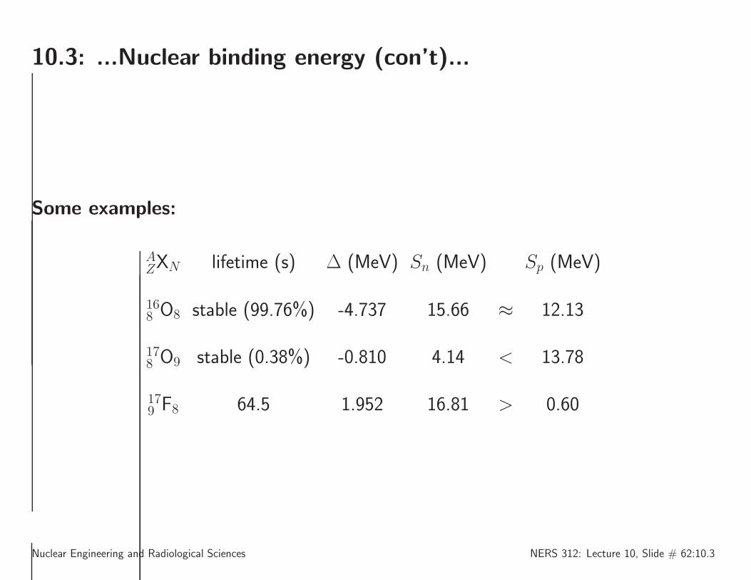
Some examples:
AZXN lifetime (s) ∆ (MeV) Sn (MeV) Sp (MeV)
168 O8 stable (99.76%) -4.737 15.66 ≈ 12.13
178 O9 stable (0.38%) -0.810 4.14 < 13.78
179 F8 64.5 1.952 16.81 > 0.60
Nuclear Engineering and Radiological Sciences NERS 312: Lecture 10, Slide # 62:10.3

10.3: ...Nuclear binding energy (con’t)...
There are:
• 82 stable (i.e.“no measurable decay rate”)20983 Bi has a measured half-life of (19± 2)× 1018 years (α-decay)!
• Those 82 stable elements have 256 stable isotopes.Sn (tin) has 28 known unstable isotopes, ranging from 99Sn–137Sn plus 10 stableisotopes ranging from 112Sn–126Sn.
• These stable isotopes, plus the more than 1000 unstable but usable nuclei (from thestandpoint of living long enough to provide a direct measurement of mass), can havetheir binding energy characterized by a universal fitting function, the semi-empiricalformula for B(Z,A) ≡ BN(Z,A), a five-parameter empirical fit to the 1000+ setof data points. (The subscript N is dropped to distinguish B as the formula derivedfrom data fitting.)
Nuclear Engineering and Radiological Sciences NERS 312: Lecture 10, Slide # 63:10.3

10.3: ...Nuclear binding energy (con’t)...
Semi-empirical Mass Formula – Binding Energy per Nucleon
The formula for B(Z,A) is given conventionally as:
B(Z,A) = aVA (“volume” term)
−aSA2/3 (“surface” term)
−aCZ(Z − 1)A−1/3 (“Coulomb repulsion” term)
−asym(A−2Z)2
A(“symmetry” term)
+ap(−1)Z [1+(−1)A]
2A−3/4 (“pairing” term) (10.38)
ai [MeV] Description Source
aV
15.5 Volume attraction Liquid Drop Model
aS
16.8 Surface repulsion Liquid Drop Model
aC
0.72 Coulomb repulsion Liquid Drop Model + Electrostatics
asym 23 n/p symmetry Shell model
ap 34 n/n, p/p pairing Shell model
Table 10.1: Fitting parameters for the nuclear binding energy
Nuclear Engineering and Radiological Sciences NERS 312: Lecture 10, Slide # 64:10.3

10.3: ...Nuclear binding energy (con’t)...
Contributions from the Liquid Drop Model
Volume attraction represents the attraction of a core nucleon to its surrounding neigh-bors... attractive, and ∝ A, since RN ∝ A1/3... comes from considering the nucleusto be an incompressible fluid of mutually-attracting nucleons, i.e. the Liquid DropModel of the nucleus
Surface attraction accounts for deficit of nuclear force saturation for surface nucleons.... repulsive, and ∝ R2
N ∝ A2/3
Coulomb repulsion is estimated from (10.28)... ∝ 1/RN ∝ A−1/3...Z2 is replaced byZ(Z − 1) since a solitary proton does not repulse itself... the electrostatic charge isconsidered to be spread uniformly through the drop.
Nuclear Engineering and Radiological Sciences NERS 312: Lecture 10, Slide # 65:10.3

10.3: ...Nuclear binding energy (con’t)...
Contributions from the Shell Model
n/p symmetry since nuclei like to form with equal numbers of protons and neutrons(Nuclear Shall Model)... ∝ [(A− 2Z)/A]2...minimizes (vanishes) when Z = N . Thisis a “Fermi pressure” term, meaning that the nucleus wants to maximize the differenceof particle types in the nucleus.
n/n, p/p pairing since the Nuclear Shell Model predicts that nuclei prefer when protonsor neutrons are paired up in n− n, p− p pairs... attractive for an even-even nucleus(both Z and N are even), repulsive for an odd-odd nucleus, and zero otherwise. TheA−3/4 comes from Shell Model calculations, and often varies in the literature. Thisterm comes from the spin-spin interaction. Like magnets (which is sort of, whatnucleons are), want to anti-align their magnetic poles.
Nuclear Engineering and Radiological Sciences NERS 312: Lecture 10, Slide # 66:10.3
10.3: ...Nuclear binding energy (con’t)...
0 20 40 60 80 100 120 140 160 180 2002
4
6
8
10
12
14
A
B(Z
min
,A)/
A (
MeV
)
Binding energy per nucleon vs. A
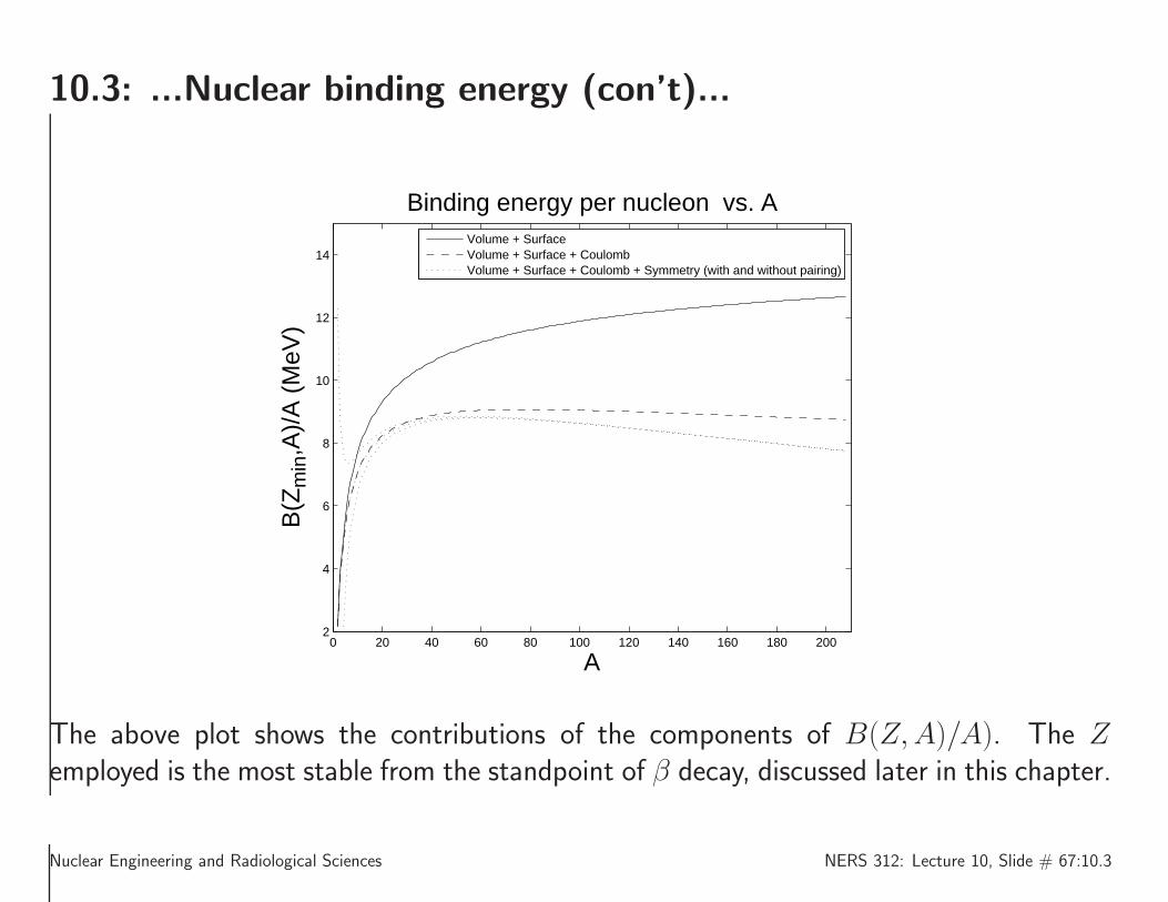
Volume + SurfaceVolume + Surface + CoulombVolume + Surface + Coulomb + Symmetry (with and without pairing)
The above plot shows the contributions of the components of B(Z,A)/A). The Zemployed is the most stable from the standpoint of β decay, discussed later in this chapter.
Nuclear Engineering and Radiological Sciences NERS 312: Lecture 10, Slide # 67:10.3
10.3: ...Nuclear binding energy (con’t)...
0 50 100 150 200 2500
1
2
3
4
5
6
7
8
9
A
B(Z
min
,A)/
A (
MeV
)
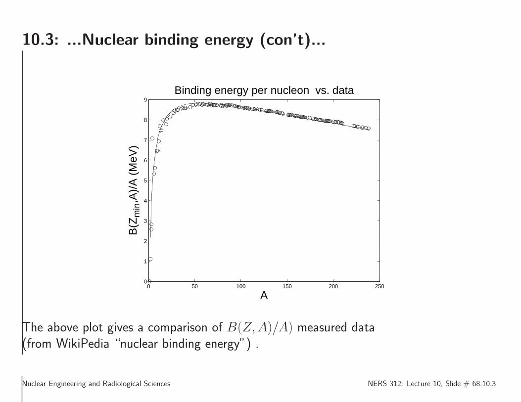
Binding energy per nucleon vs. data
The above plot gives a comparison of B(Z,A)/A) measured data(from WikiPedia “nuclear binding energy”) .
Nuclear Engineering and Radiological Sciences NERS 312: Lecture 10, Slide # 68:10.3

10.3: ...Nuclear binding energy (con’t)...
Binding Energy per Nucleon, major results
B(Z,A)/A ...
• peaks at about A = 56 (Fe). Iron and nickel (the iron core of the earth) are naturalendpoints of the fusion process.
• is about 8 MeV ± 10 % for A > 10.
Nuclear Engineering and Radiological Sciences NERS 312: Lecture 10, Slide # 69:10.3

10.3: ...Nuclear binding energy (con’t)...
Using the expression (10.38), viz.
B(Z,A) = aVA− a
SA2/3 − a
CZ(Z − 1)A−1/3 − asym
(A− 2Z)2
A
+ap(−1)Z[1 + (−1)A]
2A−3/4
and adapting (10.35), viz.
BN(Z,A) = [Zm(1H) +Nmn −m(AX)]c2
we obtain the semi-empirical mass formula:
m(AX) = Zm(1H) +Nmn −B(Z,A)/c2 , (10.39)
that one may use to estimate m(AX) from measured values of the binding energy, orvice-versa.
Nuclear Engineering and Radiological Sciences NERS 312: Lecture 10, Slide # 70:10.3

10.3: ...Nuclear binding energy (con’t)...
Application to β-decay
β-decay occurs when a proton or a neutron in a nucleus converts to the other form ofnucleon, n → p, or p → n. (An unbound neutron will also β-decay.) This processpreserves A. Therefore, one may characterize β-decay as an isobaric (i.e. same A)transition. For fixed A, (10.39) represents a parabola in Z, with the minimum occurringat (Note: There is a small error in Krane’s formula below.):
Zmin =[mn −m(1H)]c2 + a
CA−1/3 + 4asym
2aCA−1/3 + 8asymA
−1. (10.40)
We have to use some caution when using this formula. When A is odd, there is noambiguity. However, when the decaying nucleus is odd-odd, the transition picks up anadditional loss in mass of 2apA
−3/4, because an odd-odd nucleus becomes an even-evenone. Similarly, when an even-even nucleus decays to an odd-odd nucleus, it picks up again of 2apA
−3/4 in mass, that must be more than compensated for, by the energetics ofthe β-decay.
Nuclear Engineering and Radiological Sciences NERS 312: Lecture 10, Slide # 71:10.3

10.3: ...Nuclear binding energy (con’t)...
0 50 100 150 200 2500.38
0.4
0.42
0.44
0.46
0.48
0.5
0.52
ZminA−1 vs. A
Zm
inA
−1
A
Nuclear Engineering and Radiological Sciences NERS 312: Lecture 10, Slide # 72:10.3

10.3: ...Nuclear binding energy (con’t)...
Figure 3.18 in Krane illustrates this for two different decays chains.
Nuclear Engineering and Radiological Sciences NERS 312: Lecture 10, Slide # 73:10.3

10.3: ...Nuclear binding energy (con’t)...
(10.40) can very nearly be approximated by:
Zmin ≈A
2
1
1 + (1/4)(aC/asym)A
2/3. (10.41)
This shows clearly the tendency for Z ≈ N for lighter nuclei. For heavier nuclei, A ≈ 0.41.
Nuclear Engineering and Radiological Sciences NERS 312: Lecture 10, Slide # 74:10.3

10.4: Angular momentum and parity...
Some notation:
Symbol meaningli orbital angular momentum of the i’th nucleonsi intrinsic spin angular momentum of the i’th nucleon
ji total angular momentum of the i’th nucleon, i.e. ~i = ~li + ~si~L sum of all orbital angular momenta in a nucleus i.e. ~L =
∑Ai=1~li
~S sum of all intrinsic spin angular momenta in a nucleus i.e. ~S =∑A
i=1 ~si
The total angular momentum of a nucleus is formed from the sum of the individualconstituents angular momentum, ~l, and spin, ~s, angular momentum. The symbol givento the nuclear angular momentum is I .Thus,
~I =
A∑
i=1
(~li + ~si) = ~L + ~S . (10.42)
Nuclear Engineering and Radiological Sciences NERS 312: Lecture 10, Slide # 75:10.4

10.4: Angular momentum and parity...
These angular momenta add in the Quantum Mechanical sense. That is:
〈~I2〉 = ~2I(I + 1)
I = 0,1
2, 1,
3
2· · ·
〈Iz〉 = ~mI
mI
: −I ≤ mI≤ I
∆mI
: integral jumps (10.43)
Nuclear Engineering and Radiological Sciences NERS 312: Lecture 10, Slide # 76:10.4

10.4: ...Angular momentum and parity...
Since neutron and proton spins are half-integral, and orbital angular momentum is integral,it follows that I is half-integral for odd-A nuclei, and integral for even-A nuclei.Recall that parity is associated with a quantum number of ±1, that is associated with theinversion of space. That is, if Π is the parity operator, acting on the composite nuclearwave function, Ψ(~x;A,Z),
ΠΨ(~x;A,Z) = ±Ψ(−~x;A,Z) . (10.44)
The plus sign is associated with “even parity” and the minus sign with “odd parity”.Total spin and parity are measurable, and a nucleus is said to be in an Iπ configuration.For example, 235U has Iπ = 7
2
−, while 238U has Iπ = 0+.
Nuclear Engineering and Radiological Sciences NERS 312: Lecture 10, Slide # 77:10.4

10.4: ...Angular momentum and parity...
• If the nuclear strong force were completely central, i.e. V (~x) = V (r), thenL, ML, S, MS would all be constants of the motion.
• In atomic physics, and nuclear physics, the spin-orbit force has the form Vso(r)~l · ~s.However, in atomic physics, this effect is small, and splits the spectroscopy lines by asmall amount (called the “fine” structure).
• In atomic physics, and nuclear physics, the spin-spin force has the form Vss(r)~s · ~s.However, in atomic physics, this effect is even smaller, and splits the spectroscopylines by a smaller amount (call the “hyperfine” structure).
• However, in nuclear physics, these forces are very strong, and can not be treated assmall perturbations, leading to great mathematical complexity. Moreover, L, ML,S, MS are not constants of the motion. This has interesting effect, that we shallencounter later. But, total angular momentum, I , is a constant for each nucleus.
• Observational fact: All the even-even nuclei have I = 0, because of the strong pairingforce.
Nuclear Engineering and Radiological Sciences NERS 312: Lecture 10, Slide # 78:10.4

10.5: Nuclear magnetic and electric moments...
An illustration of the preferred spin orientations of the up, down, and strange quarks andantiquarks within a polarized proton. From “The Frontiers of Nuclear Science — A LongRange Plan, December 2007”, by the Nuclear Science Advisory Committee.
An introduction to moments is given in terms of the gravitational force. The handwrittennotes are in Chapter10.pdf, in pdf pages 55-60.
Nuclear Engineering and Radiological Sciences NERS 312: Lecture 10, Slide # 79:10.5

10.6: ...Nuclear magnetic and electric moments...
This is the dipole magnetic field, ~B and the “dipole moment”, ~m or ~µ of a permanentmagnet.
Nuclear Engineering and Radiological Sciences NERS 312: Lecture 10, Slide # 80:10.6

10.7: ...Nuclear magnetic and electric moments...
A moving charge (positive in this case) generates a similar magnetic field and dipolemoment. For a negative charge moving in the same direction, the direction of the magneticmoment would be reversed.
Nuclear Engineering and Radiological Sciences NERS 312: Lecture 10, Slide # 81:10.7
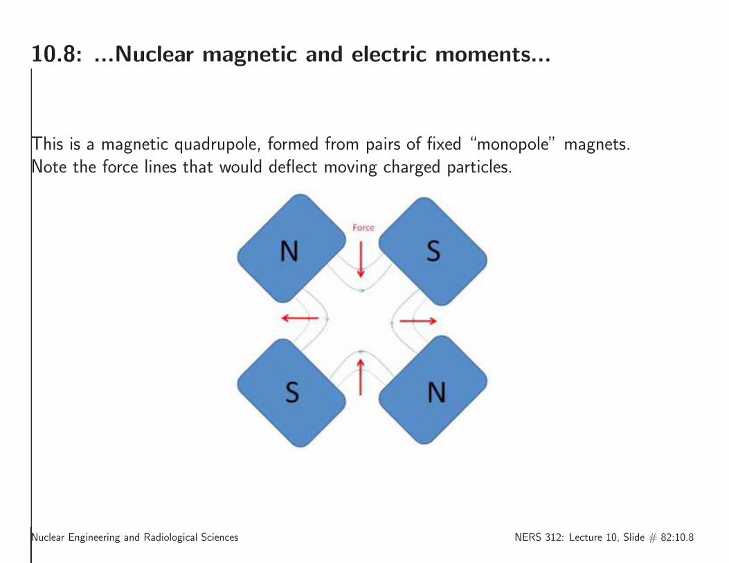
10.8: ...Nuclear magnetic and electric moments...
This is a magnetic quadrupole, formed from pairs of fixed “monopole” magnets.Note the force lines that would deflect moving charged particles.
Nuclear Engineering and Radiological Sciences NERS 312: Lecture 10, Slide # 82:10.8

10.9: ...Nuclear magnetic and electric moments...
Magnetic monopoles do not exist in nature, so quadrupole magnets are made up of 4opposing dipole magnets, in this illustration, electromagnets.
Nuclear Engineering and Radiological Sciences NERS 312: Lecture 10, Slide # 83:10.9

10.10: ...Nuclear magnetic and electric moments...
Pairs of quadrupole magnets, in opposing orientations form a quadrupole lens, used forfocusing beams of charged particles. You can see some of these in the MIBL. (This oneis from the Maier-Leibnitz lab in Munich.
Nuclear Engineering and Radiological Sciences NERS 312: Lecture 10, Slide # 84:10.10

10.10.1: Magnetic dipole of nucleons...
Nucleons, in a tightly-bound nucleus, all in close proximity to each other, all moving withvelocities of about 0.001 → 0.1c. This is a radical departure from the leisurely orbit ofan electron about a nucleus. This is a “mosh pit” of thrashing, slamming nucleons. Theforces between them are considerable, and play a vital role in the determination of nuclearstructure.
The orbital angular momentum can be characterized in classical electrodynamics in termsof a magnetic moment, ~µ:
~µ =1
2
∫
d~x ~x× ~J(~x) , (10.45)
where ~J(~x) is the current density. For the purpose of determining the orbital angularmomentum’s contribution to the magnetic moment, the nucleons can be considered to bepoint-like particles.
Nuclear Engineering and Radiological Sciences NERS 312: Lecture 10, Slide # 85:10.10
10.10.1: ...Magnetic dipole of nucleons...
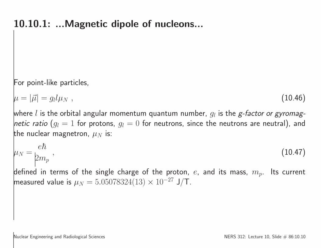
For point-like particles,
µ = |~µ| = gllµN , (10.46)
where l is the orbital angular momentum quantum number, gl is the g-factor or gyromag-netic ratio (gl = 1 for protons, gl = 0 for neutrons, since the neutrons are neutral), andthe nuclear magnetron, µN is:
µN =e~
2mp, (10.47)
defined in terms of the single charge of the proton, e, and its mass, mp. Its currentmeasured value is µN = 5.05078324(13)× 10−27 J/T.
Nuclear Engineering and Radiological Sciences NERS 312: Lecture 10, Slide # 86:10.10
10.10.1: ...Magnetic dipole of nucleons...
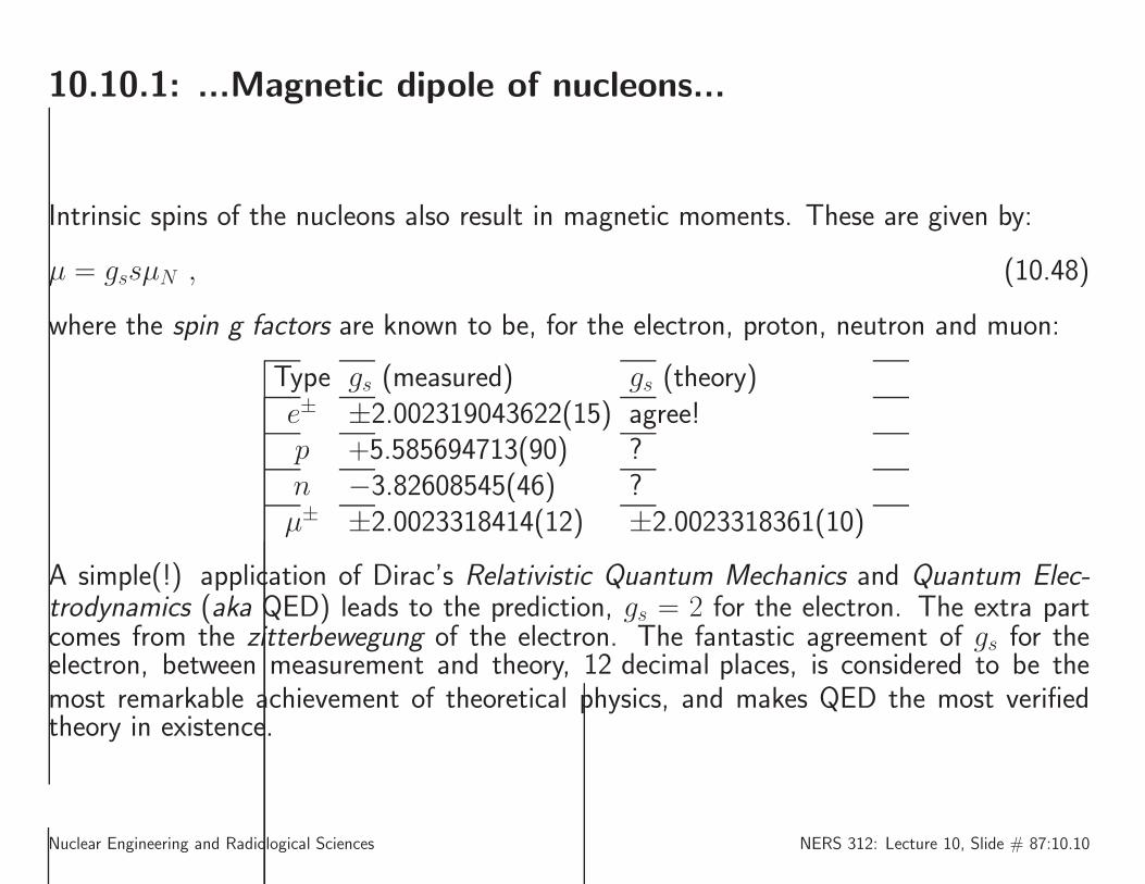
Intrinsic spins of the nucleons also result in magnetic moments. These are given by:
µ = gssµN , (10.48)
where the spin g factors are known to be, for the electron, proton, neutron and muon:
Type gs (measured) gs (theory)e± ±2.002319043622(15) agree!p +5.585694713(90) ?n −3.82608545(46) ?µ± ±2.0023318414(12) ±2.0023318361(10)
A simple(!) application of Dirac’s Relativistic Quantum Mechanics and Quantum Elec-trodynamics (aka QED) leads to the prediction, gs = 2 for the electron. The extra partcomes from the zitterbewegung of the electron. The fantastic agreement of gs for theelectron, between measurement and theory, 12 decimal places, is considered to be themost remarkable achievement of theoretical physics, and makes QED the most verifiedtheory in existence.
Nuclear Engineering and Radiological Sciences NERS 312: Lecture 10, Slide # 87:10.10
10.10.1: ...Magnetic dipole of nucleons...
• There is no theory for the determination of the nucleon g-factors. However, themeasured values allow us to reach an important conclusion: The proton must besomething very different from a point charge (else its gs would be close to 2), and theneutron must be made up of internal charged constituents (else its gs would be 0).
• These observations laid the groundwork for further investigation that ultimately ledto the discovery (albeit indirectly), that neutrons and protons are made up of quarks.(Free quarks have never been observed.) This led to the development of QuantumChromodynamics (aka QCD), that describes the the strong force in fundamental,theoretical terms. The unification of QCD, QED, and the weak force (responsible forβ-decay) is called The Standard Model of particle physics.
• Measurement and Theory differ, however, for the muon’s gs. It has been suggestedthat there is physics beyond The Standard Model that accounts for this.
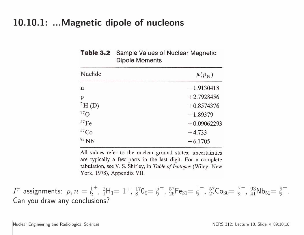
• Table 3.2 in Krane provides some examples. Further exploration awaits our laterdiscussions on nuclear models.
Nuclear Engineering and Radiological Sciences NERS 312: Lecture 10, Slide # 88:10.10
10.10.1: ...Magnetic dipole of nucleons
Iπ assignments: p, n = 12
+, 21H1= 1+, 17
8 09=52
+, 5726Fe31=
12
−, 5727Co30=
72
−, 9341Nb52=
92
+.
Can you draw any conclusions?
Nuclear Engineering and Radiological Sciences NERS 312: Lecture 10, Slide # 89:10.10

10.10.2: Quadrupole moments of nuclei...
The electric quadrupole moment is derived from the following considerations.The electrostatic potential of the nucleus is given by:
V (~x) =Ze
4πǫ0
∫
d~x′ρp(~x
′)
|~x− ~x′| . (10.49)
Now, imagine that we are probing the nucleus from a considerable distance, so far awayfrom it, that we can only just discern the merest details of its shape. Given that ρp(~x
′)is highly localized in the vicinity of the nucleus and our probe is far removed from it, wemay expand (10.49) in a Taylor expansion in |~x′|/|~x|. Thus we obtain:
V (~x) =Ze
4πǫ0
[
1
|~x|
∫
d~x′ ρp(~x′) +
~x
|~x|3 ·∫
d~x′ ~x′ρp(~x′)+
1
2|~x|5∫
d~x′(
3(~x · ~x′)2 − |~x|2|~x′|2)
ρp(~x′) · · ·
]
. (10.50)
Nuclear Engineering and Radiological Sciences NERS 312: Lecture 10, Slide # 90:10.10

10.10.2: Quadrupole moments of nuclei...
This simplifies to:
V (~x) =Ze
4πǫ0
[
1
|~x| +Q
2|~x|3 · · ·]
, (10.51)
where
Q =
∫
d~x(
3z2 − r2)
ρp(~x) . (10.52)
We have used∫
d~x ρp(~x) ≡ 1 for the first integral in (10.50). This is simply a statementof our conventional normalization of ρp(~x). We also used
∫
d~x ~xρp(~x) ≡ 0 in the secondintegral in (10.50). This is made possible by choosing the “center of charge” as the originof the coordinate system for the integral. Finally, the third integral resulting in (10.52),arises from the conventional choice, when there is no preferred direction in a problem, andset the direction of ~x′ to align with the z′-axis, for mathematical convenience.
Nuclear Engineering and Radiological Sciences NERS 312: Lecture 10, Slide # 91:10.10

10.10.2: Quadrupole moments of nuclei...
Technical note: The second integral can be made to vanish through the choice of a centerof charge. This definition is made possible because the charge is of one sign. Generally,when charges of both signs are involved in an electrostatic configuration, and their re-spective centers of charge are different, the result is a non-vanishing term known as theelectric dipole moment. In this case, the dipole moment is given by:
~d =
∫
d~x′ ~x′ρ(~x′) .
Finally, when it is not possible to choose the z-axis to be defined by the direction of ~x,but instead, by other considerations, the quadrupole becomes a tensor, with the form:
Vq(~x) =Ze
4πǫ0
1
|~x|31
2
∑
i,j
Qijninj ,
where
Qij =
∫
d~x(
3x′ix′j − δij|~x′|2
)
ρp(~x′) .
Here the quadrupole part of the potential is Vq(~x) and the ni are the 3 direction compo-nents from the center of mass of the charged object to the point where Vq(~x) is measured.Note that |n| = 1.
Nuclear Engineering and Radiological Sciences NERS 312: Lecture 10, Slide # 92:10.10

10.10.2: Quadrupole moments of nuclei...
The quantum mechanics analog to (10.52) is:
Q =
∫
d~x ψ∗N(~x)(3z
2 − r2)ψN(~x) , (10.53)
where ψN(~x) is the composite nuclear wave function. The electric quadrupole momentof the nucleus is also a physical quantity that can be measured, and predicted by nuclearmodel theories. See Krane’s Table 3.3.
Nuclear Engineering and Radiological Sciences NERS 312: Lecture 10, Slide # 93:10.10

10.10.2: Quadrupole moments of nuclei...
Nuclear Engineering and Radiological Sciences NERS 312: Lecture 10, Slide # 94:10.10

10.11:Nuclear excited states
Nuclear Engineering and Radiological Sciences NERS 312: Lecture 10, Slide # 95:10.11
Chapter 10: Nuclear Properties...
Things to think about ...
Chapter 10.0: Introduction ...
1. Describe the charge distribution of the p and n. What do those charge distributionsimply?
2. Sketch the repulsive and attractive parts of the nucleon-nucleon force. Add themtogether, and sketch that.
3. Recall the components of the nucleon-nucleon force.
4. How are nuclei formed?
Chapter 10.1: The nuclear radius ...
1. What projectile is ideal to probe the nuclear charge distribution? What should itsenergy be?
2. What is momentum transfer? Form factor?
3. What is the characteristic shape of a form factor? What does it mean?
4. How are form factors used to measure the nuclear charge distribution?
Nuclear Engineering and Radiological Sciences NERS 312: Lecture 10, Slide # 96:10.11

Chapter 10: Nuclear Properties...
Chapter 10.1: ...The nuclear radius ...
5. Is the nuclear charge distribution and the nuclear density distribution the same?(Apart from a normalization factor.)
6. What is the Woods-Saxon model of the nuclear charge density?
7. What is RN , R0, and their approximate values?
8. Where does the simple model for RN break down? Why?
9. How can the size of the nucleus be determine from K-shell decays?
10. What is the “isotope” shift?
11. Why are muonic atoms a great tool in these measurements?
12. How can one measure the charge radius of a nucleus from the Coulomb energy inmirror nuclei? How does this experiment work?
13. Show that(
3
4π
)2 ∫
|~u1|≤1
d~u1
∫
|~u2|≤1
d~u21
|~u1 − ~u2|=
6
5
and describe why this integral is so important in nuclear physics. Where does itcome from?
Nuclear Engineering and Radiological Sciences NERS 312: Lecture 10, Slide # 97:10.11

Chapter 10: Nuclear Properties...
Chapter 10.3: Nuclear Binding Energy ...
1. Describe in words, what is the binding energy of the nucleus.
2. Why is atomic binding ignored in all discussions of nuclear binding energy?
3. Explain: BN(Z,A) =
Zmp +Nmn −[
m(AX)− Zme
]
c2.
4. “mass defect/mass excess” What is it?
5. What is the “neutron separation energy”?
6. What is the “proton separation energy”?
7. What is and explain B(Z,A), B(Z,A)/A and the “Semiempirical Mass Formula”
8. Explain and justify, all the components of B(Z,A).
9. Sketch B(Z,A)/A.
10. How is B(Z,A) applied to the energetics of β-decay?
Chapter 10.4: Angular Momentum and Parity ...
1. What do ~s, ~l, ~j, ~S, ~L, ~I mean? How do you calculate/determine/measure them?How do you add them?
2. What does Iπ mean? Are these unique for every isotope? What resource can youuse to find them?
Nuclear Engineering and Radiological Sciences NERS 312: Lecture 10, Slide # 98:10.11
Chapter 10: Nuclear Properties...
Chapter 10.5: Nuclear Magnetic and Electric Moments ...
1. Why can you see only one face of the moon? What percentage of the moon’ssurface can you see from the earth? What is “libration”?
2. What is a magnetic dipole?
3. Why doesn’t a nucleus have an electric dipole moment?
4. What is a quadrupole moment?
5. What are the orbital and spin gyromagnetic factors? What are the values of theangular (not the spin) ones?
6. Show that
V (~x) = lim|~x|≫RN
Ze
4πǫ0
∫
d~x′ρp(~x
′)
|~x− ~x′|
=Ze
4πǫ0
[
1
|~x|
∫
d~x′ ρp(~x′) +
~x
|~x|3 ·∫
d~x′ ~x′ρp(~x′)+
1
2|~x|5∫
d~x′(
3(~x · ~x′)2 − |~x|2|~x′|2)
ρp(~x′) · · ·
]
Nuclear Engineering and Radiological Sciences NERS 312: Lecture 10, Slide # 99:10.11