NEP “Microwave Design” Module

1

NEP “MICROWAVE DESIGN” MODULEDay 1

2

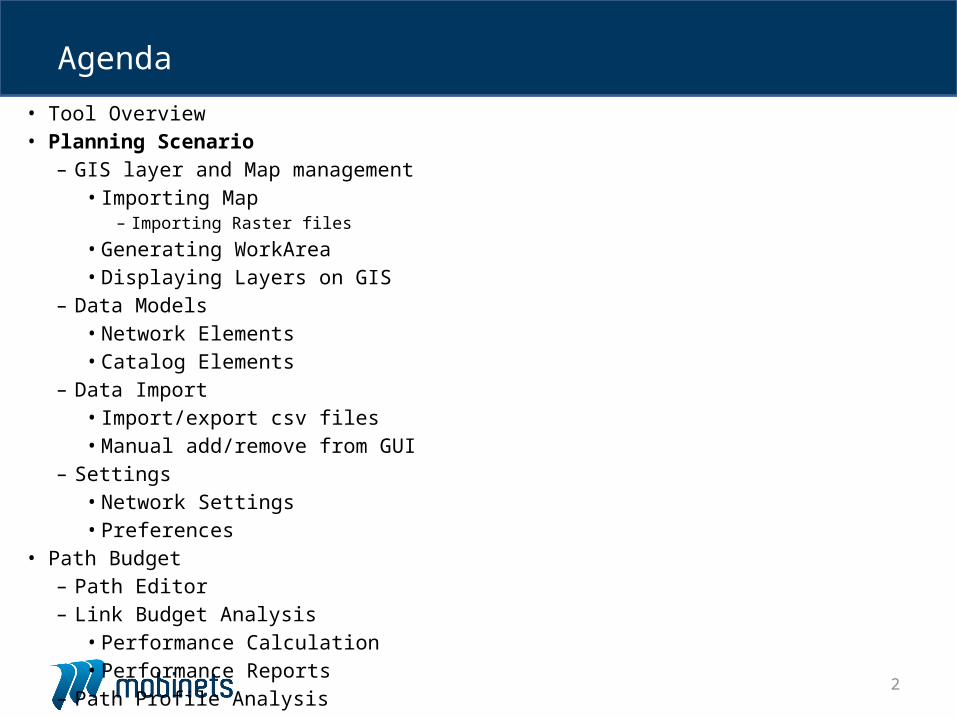
• Tool Overview• Planning Scenario

– GIS layer and Map management• Importing Map

– Importing Raster files

• Generating WorkArea• Displaying Layers on GIS

– Data Models • Network Elements• Catalog Elements

– Data Import • Import/export csv files• Manual add/remove from GUI

– Settings• Network Settings• Preferences

• Path Budget– Path Editor– Link Budget Analysis

• Performance Calculation• Performance Reports

– Path Profile Analysis

Agenda

3

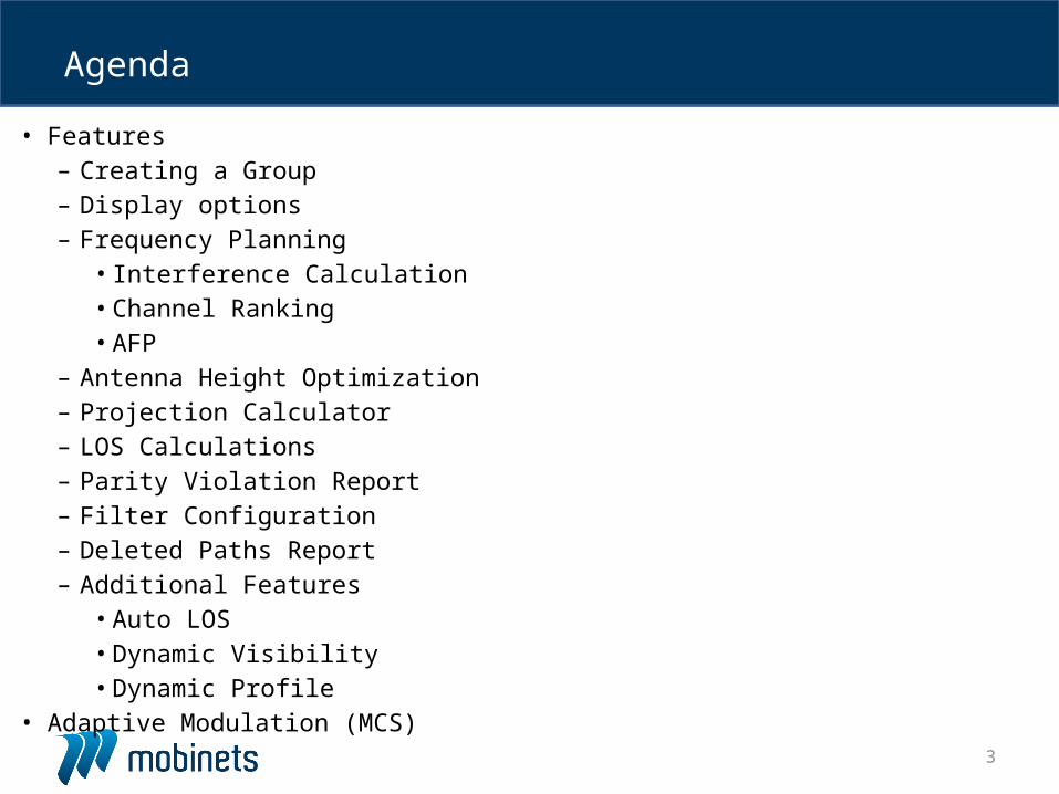
• Features – Creating a Group– Display options– Frequency Planning

• Interference Calculation • Channel Ranking • AFP

– Antenna Height Optimization– Projection Calculator– LOS Calculations– Parity Violation Report– Filter Configuration– Deleted Paths Report– Additional Features

• Auto LOS• Dynamic Visibility• Dynamic Profile

• Adaptive Modulation (MCS)

Agenda

4

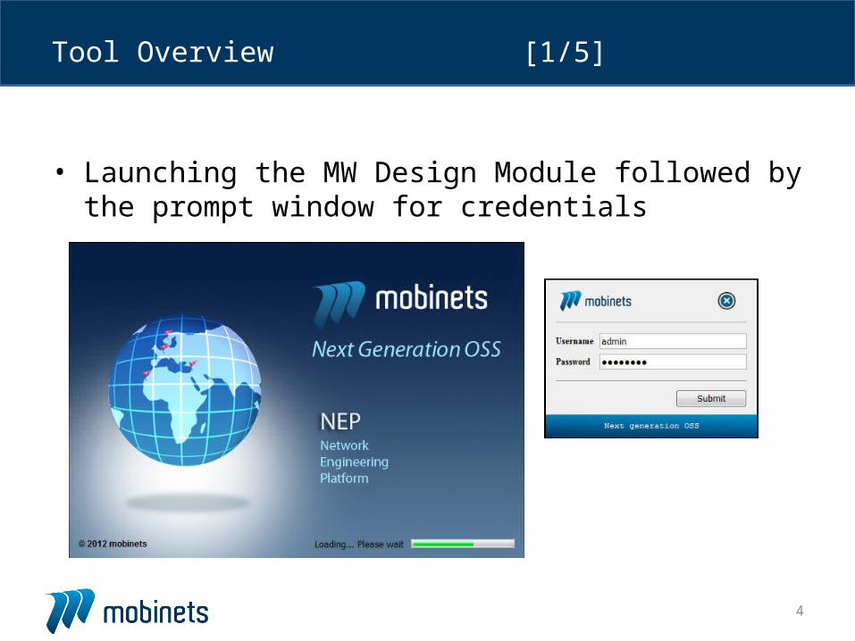
Tool Overview [1/5]

• Launching the MW Design Module followed by the prompt window for credentials

5

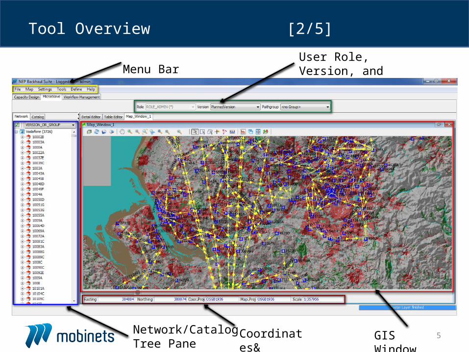
Tool Overview [2/5]

Menu BarUser Role, Version, and Group Name

GIS WindowNetwork/Catalog Tree Pane

Coordinates& Projection

6

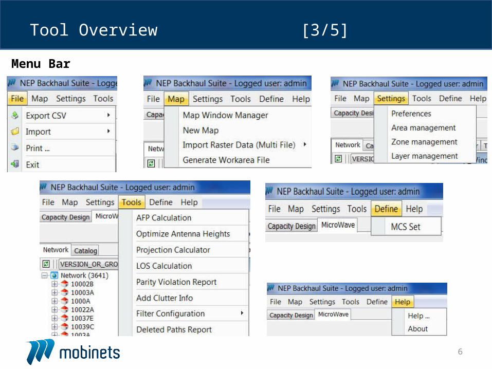
Tool Overview [3/5]

Menu Bar

7

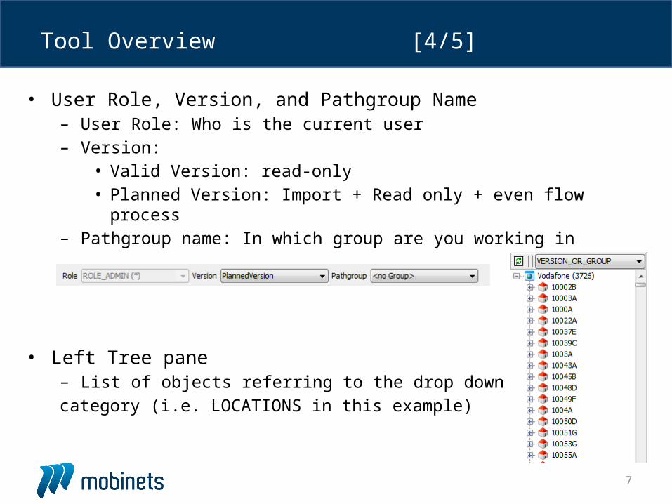
• User Role, Version, and Pathgroup Name– User Role: Who is the current user– Version:

• Valid Version: read-only• Planned Version: Import + Read only + even flow process

– Pathgroup name: In which group are you working in

• Left Tree pane– List of objects referring to the drop down menu

category (i.e. LOCATIONS in this example)

Tool Overview [4/5]

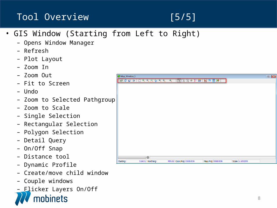
8

• GIS Window (Starting from Left to Right)– Opens Window Manager– Refresh– Plot Layout– Zoom In– Zoom Out– Fit to Screen– Undo– Zoom to Selected Pathgroup– Zoom to Scale– Single Selection– Rectangular Selection– Polygon Selection– Detail Query– On/Off Snap– Distance tool– Dynamic Profile– Create/move child window– Couple windows– Flicker Layers On/Off

Tool Overview [5/5]

9

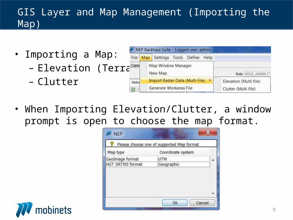
• Importing a Map:– Elevation (Terrain)– Clutter

• When Importing Elevation/Clutter, a window prompt is open to choose the map format.

GIS Layer and Map Management (Importing the Map)

10

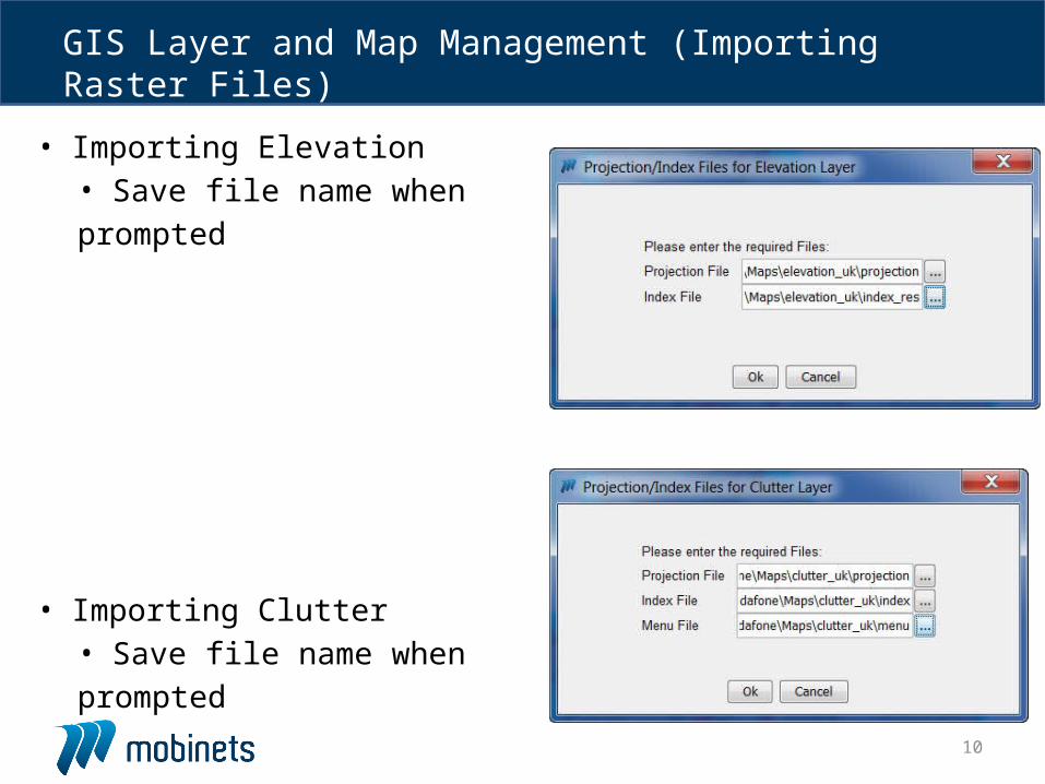
• Importing Elevation• Save file name when

prompted

• Importing Clutter• Save file name when

prompted

GIS Layer and Map Management (Importing Raster Files)

11

GIS Layer and Map Management (Generating Workarea)

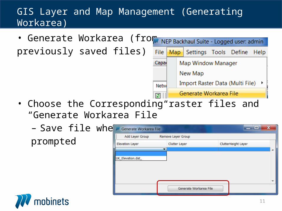
• Generate Workarea (from

previously saved files)

• Choose the Corresponding raster files and “Generate Workarea File”– Save file when

prompted

12

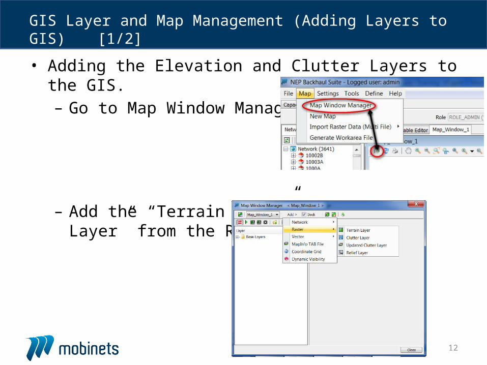
• Adding the Elevation and Clutter Layers to the GIS.– Go to Map Window Manager

– Add the “Terrain Layer” and “Clutter Layer” from the Raster as shown

GIS Layer and Map Management (Adding Layers to GIS) [1/2]

13

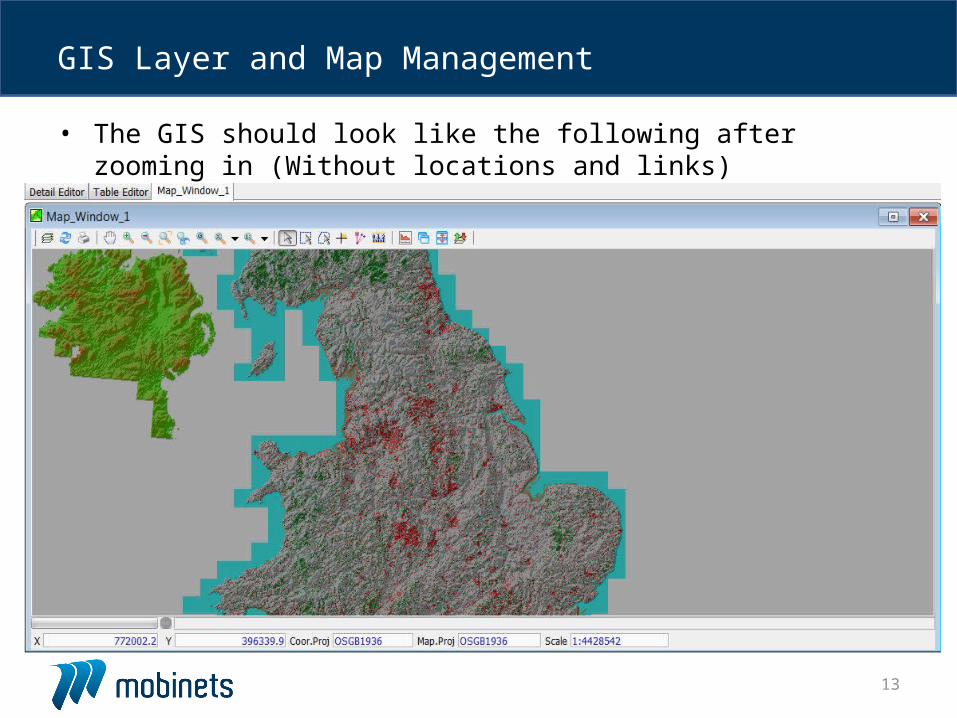
• The GIS should look like the following after zooming in (Without locations and links)

GIS Layer and Map Management

14

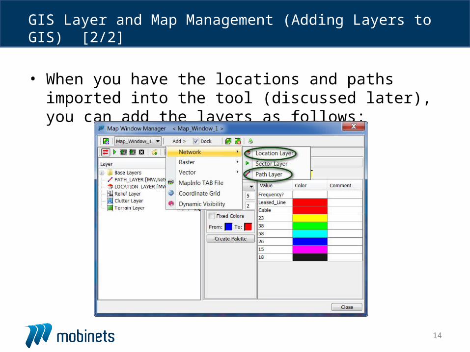
• When you have the locations and paths imported into the tool (discussed later), you can add the layers as follows:

GIS Layer and Map Management (Adding Layers to GIS) [2/2]

15

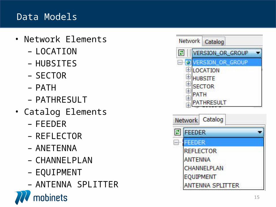
• Network Elements– LOCATION– HUBSITES– SECTOR– PATH– PATHRESULT

• Catalog Elements– FEEDER– REFLECTOR – ANETENNA– CHANNELPLAN– EQUIPMENT– ANTENNA SPLITTER

Data Models

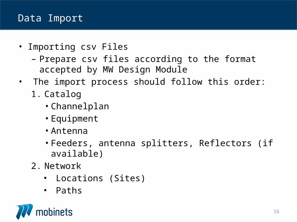
16

• Importing csv Files– Prepare csv files according to the format accepted by

MW Design Module• The import process should follow this order:

1. Catalog• Channelplan• Equipment• Antenna• Feeders, antenna splitters, Reflectors (if available)

2. Network• Locations (Sites)• Paths

Data Import

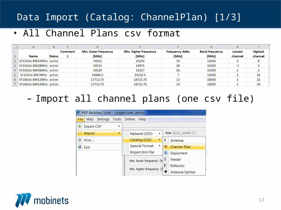
17

• All Channel Plans csv format

– Import all channel plans (one csv file)

Data Import (Catalog: ChannelPlan) [1/3]

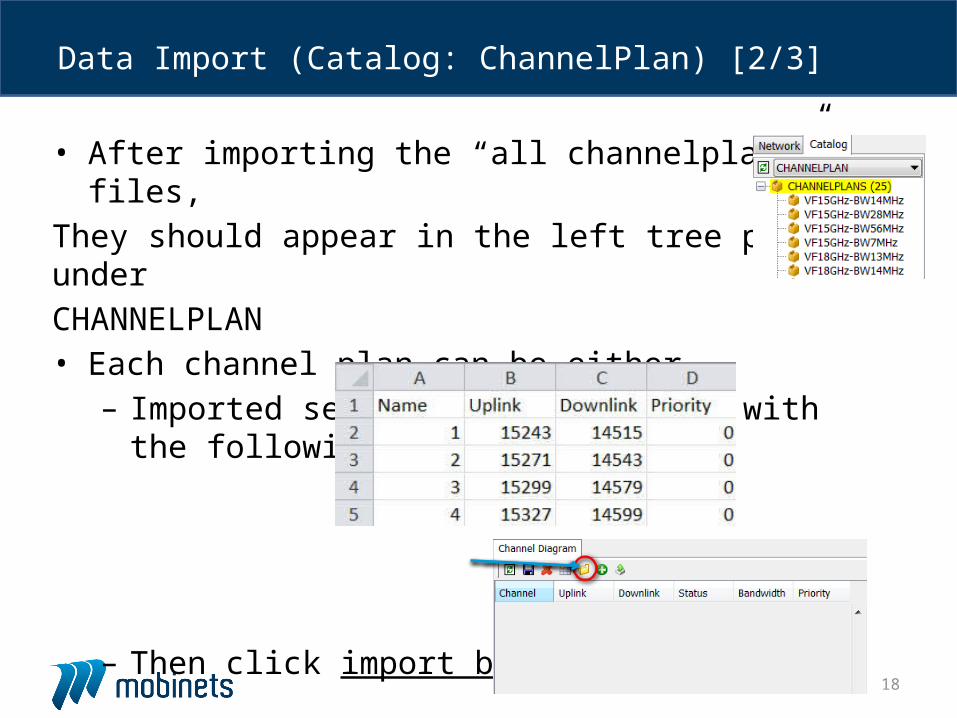
18

• After importing the “all channelplans” csv files,

They should appear in the left tree pane under

CHANNELPLAN• Each channel plan can be either

– Imported separately in csv file with the following format

– Then click import button


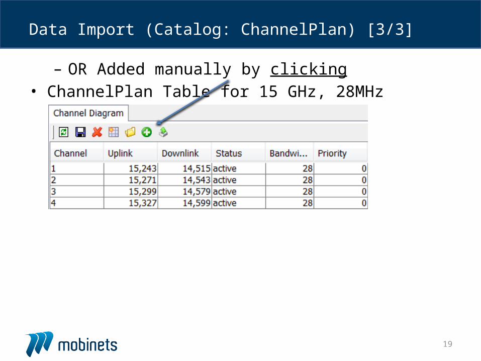
19

– OR Added manually by clicking• ChannelPlan Table for 15 GHz, 28MHz


20

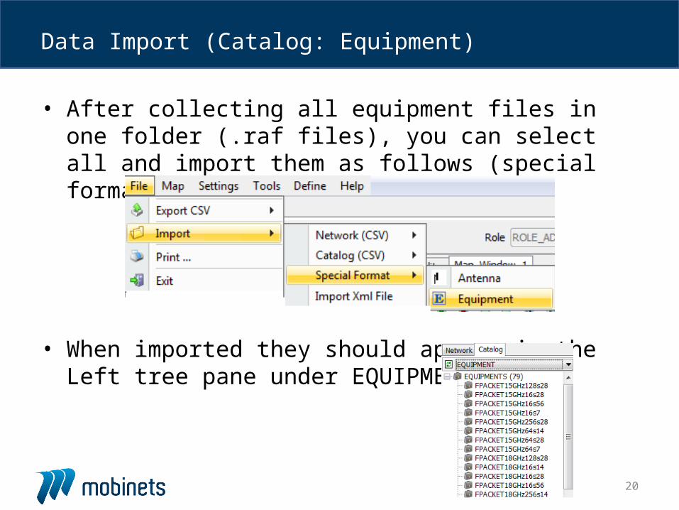
• After collecting all equipment files in one folder (.raf files), you can select all and import them as follows (special format).

• When imported they should appear in the Left tree pane under EQUIPMENT

Data Import (Catalog: Equipment)

21

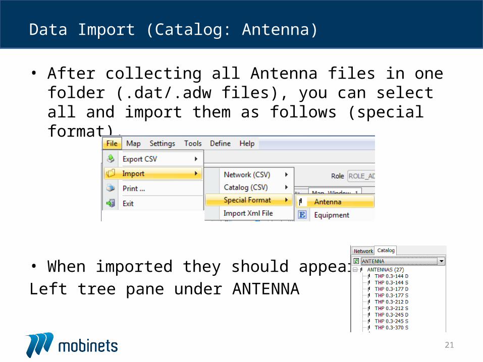
• After collecting all Antenna files in one folder (.dat/.adw files), you can select all and import them as follows (special format).

• When imported they should appear in the

Left tree pane under ANTENNA

Data Import (Catalog: Antenna)

22

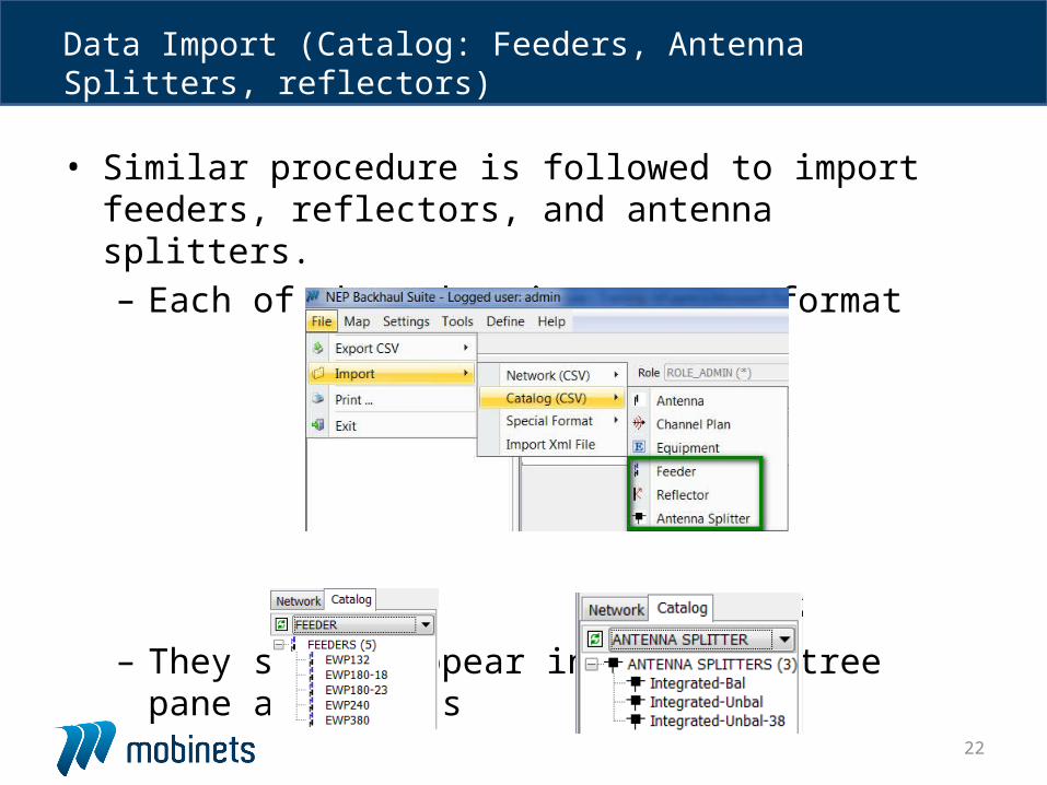
• Similar procedure is followed to import feeders, reflectors, and antenna splitters.– Each of these has its own csv format

– They should appear in the left tree pane afterwards

Data Import (Catalog: Feeders, Antenna Splitters, reflectors)

23

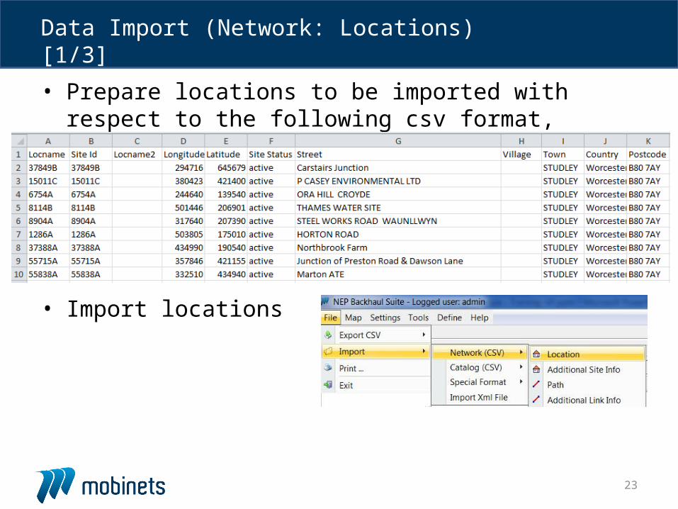
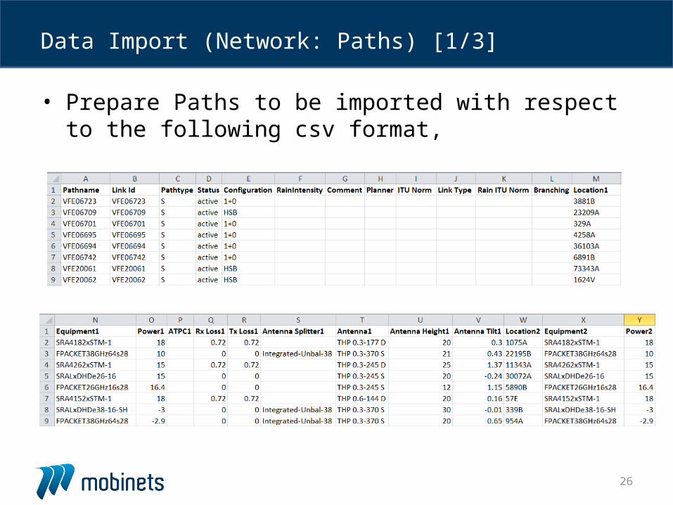
• Prepare locations to be imported with respect to the following csv format,

• Import locations

Data Import (Network: Locations) [1/3]

24

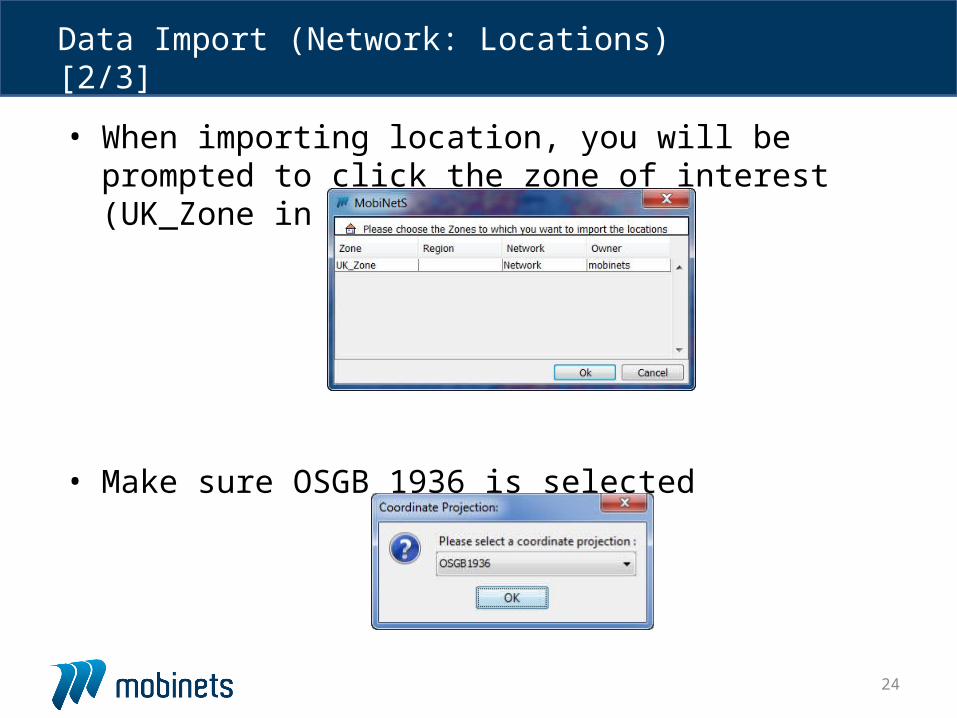
• When importing location, you will be prompted to click the zone of interest (UK_Zone in our case)

• Make sure OSGB 1936 is selected


25

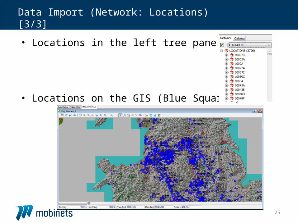
• Locations in the left tree pane

• Locations on the GIS (Blue Squares)


26

• Prepare Paths to be imported with respect to the following csv format,

Data Import (Network: Paths) [1/3]

27

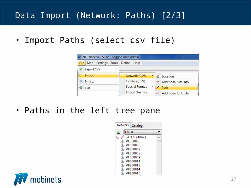
• Import Paths (select csv file)

• Paths in the left tree pane


28

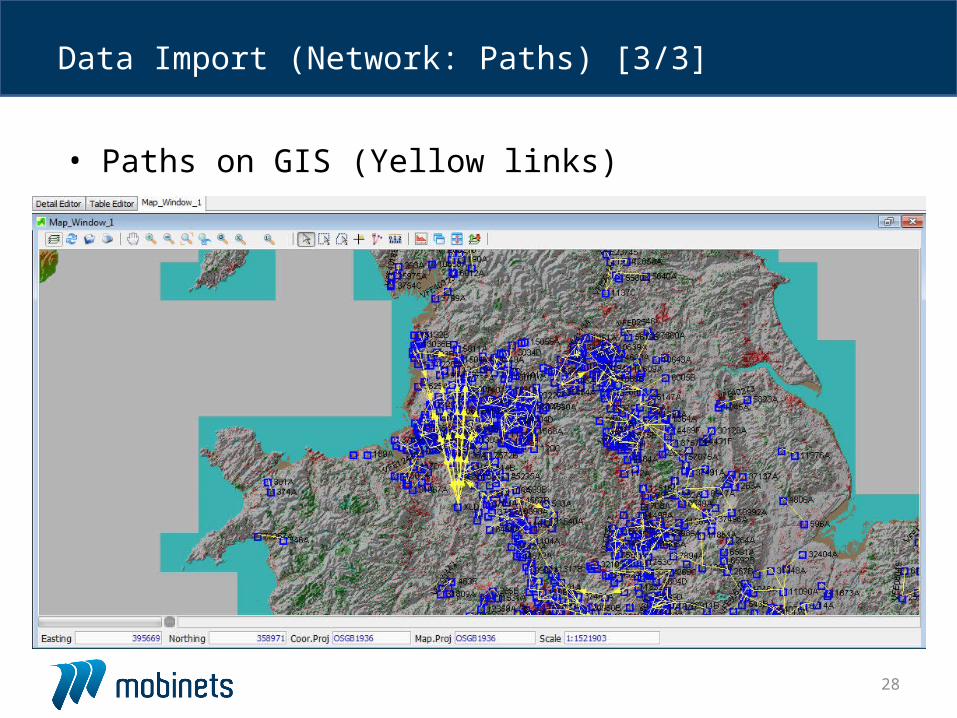
• Paths on GIS (Yellow links)


29

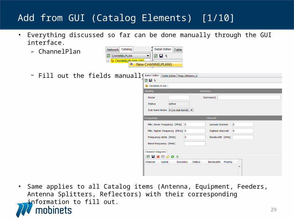
• Everything discussed so far can be done manually through the GUI interface.– ChannelPlan

– Fill out the fields manually

• Same applies to all Catalog items (Antenna, Equipment, Feeders, Antenna Splitters, Reflectors) with their corresponding information to fill out.

Add from GUI (Catalog Elements) [1/10]

30

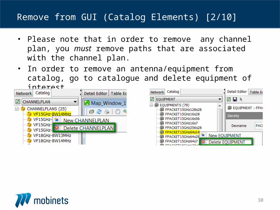
• Please note that in order to remove any channel plan, you must remove paths that are associated with the channel plan.

• In order to remove an antenna/equipment from catalog, go to catalogue and delete equipment of interest.

Remove from GUI (Catalog Elements) [2/10]

31

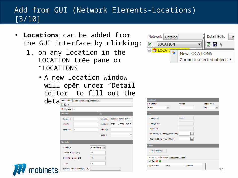
• Locations can be added from the GUI interface by clicking:

1. on any location in the LOCATION tree pane or “LOCATIONS”• A new Location window will open

under “Detail Editor” to fill out the details

Add from GUI (Network Elements-Locations) [3/10]

32

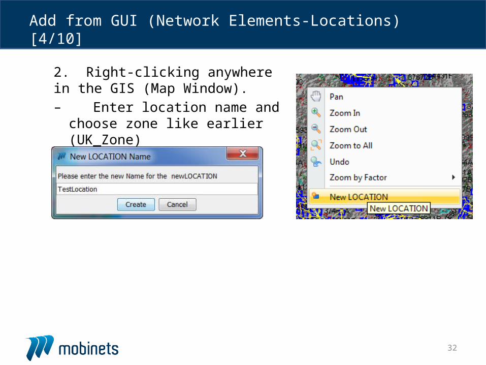
2. Right-clicking anywhere in the GIS (Map Window).– Enter location name and

choose zone like earlier (UK_Zone)

Add from GUI (Network Elements-Locations) [4/10]

33

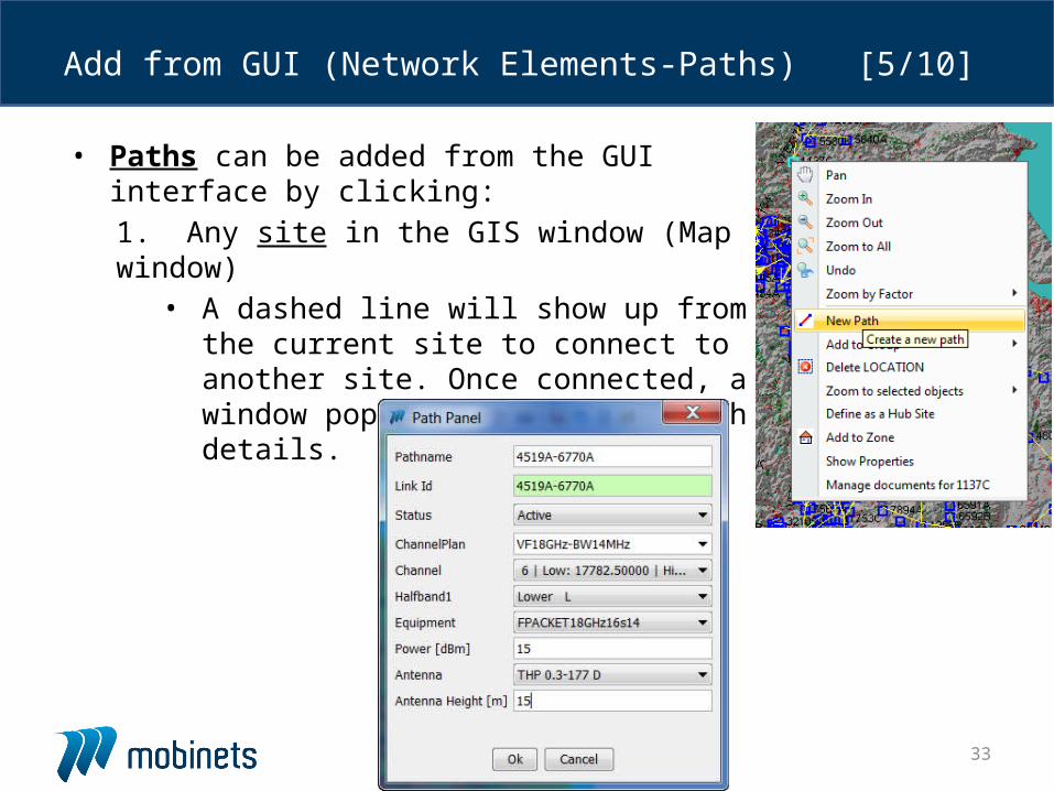
• Paths can be added from the GUI interface by clicking:

1. Any site in the GIS window (Map window)• A dashed line will show up from the

current site to connect to another site. Once connected, a window pops up to fill the path details.

Add from GUI (Network Elements-Paths)[5/10]

34

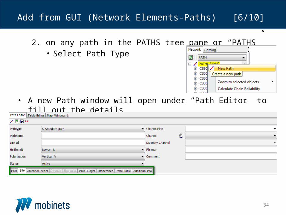
2. on any path in the PATHS tree pane or “PATHS”• Select Path Type

• A new Path window will open under “Path Editor” to fill out the details


35

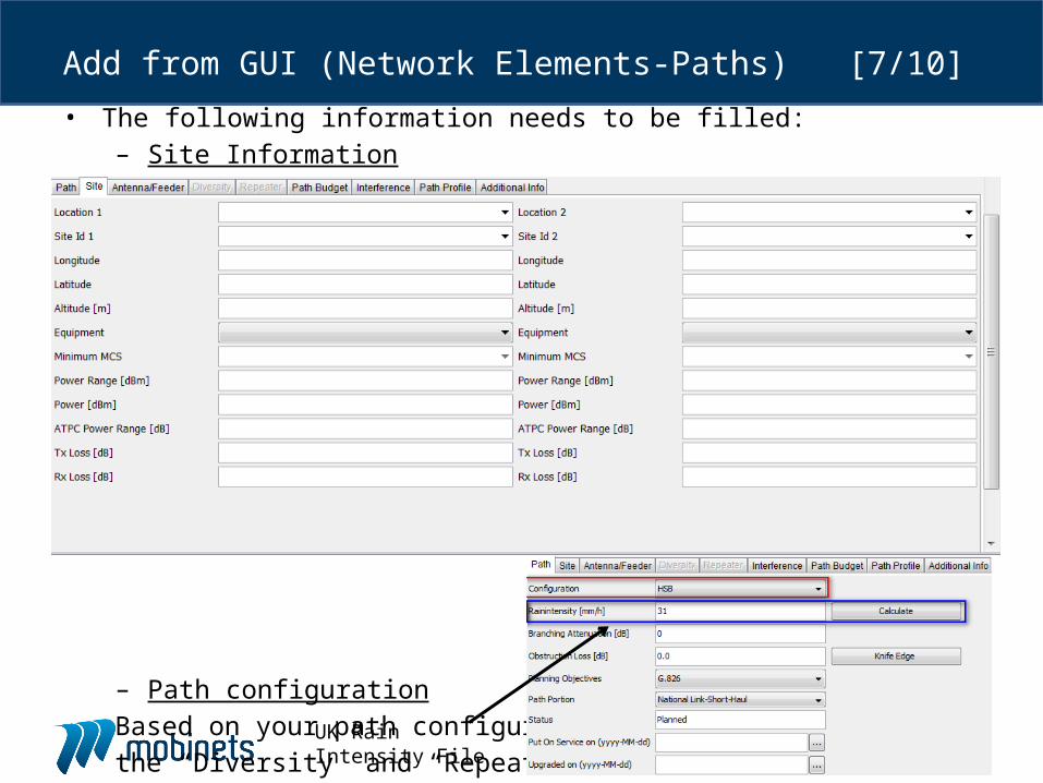
• The following information needs to be filled:– Site Information

– Path configuration

Based on your path configuration

the “Diversity” and “Repeater” tabs

get enabled.


UK Rain Intensity File

36

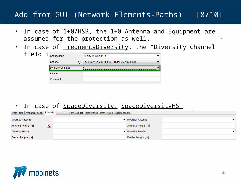
• In case of 1+0/HSB, the 1+0 Antenna and Equipment are assumed for the protection as well.

• In case of FrequencyDiversity, the “Diversity Channel” field is enabled.

• In case of SpaceDiversity, SpaceDiversityHS, Combined2RxDiversity, Combined4RxDiversity, and HSB+SD, “the Diversity” tab is enabled.


37

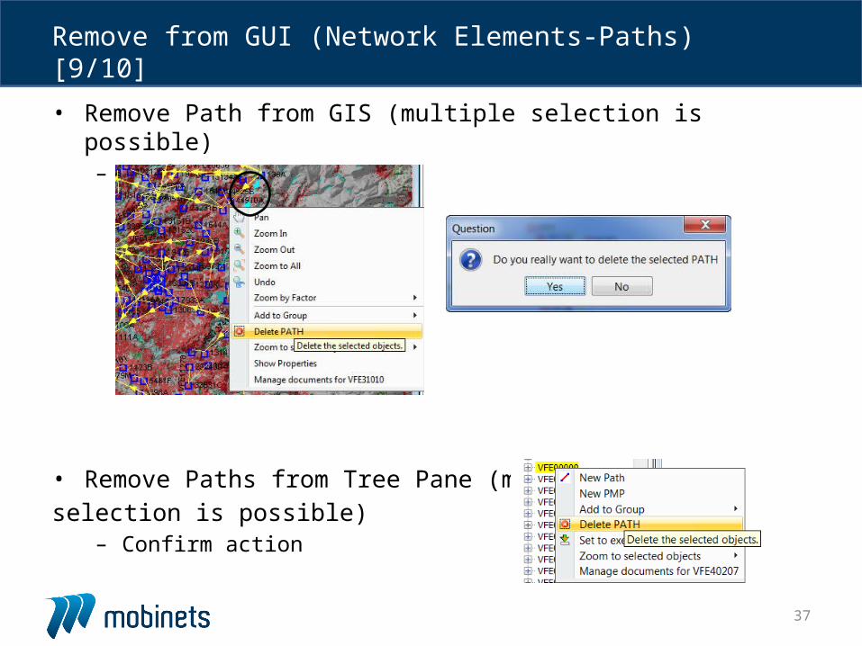
• Remove Path from GIS (multiple selection is possible)– Confirm action

• Remove Paths from Tree Pane (multiple

selection is possible)– Confirm action

Remove from GUI (Network Elements-Paths) [9/10]

38

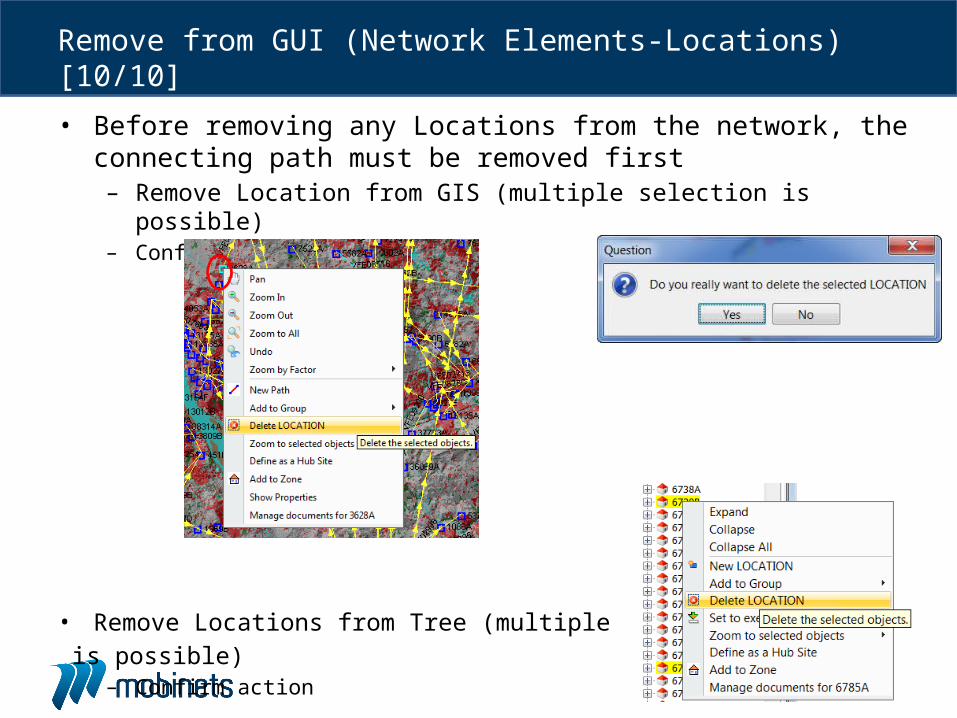
• Before removing any Locations from the network, the connecting path must be removed first– Remove Location from GIS (multiple selection is possible)– Confirm action

• Remove Locations from Tree (multiple selection

is possible)– Confirm action

Remove from GUI (Network Elements-Locations) [10/10]

39

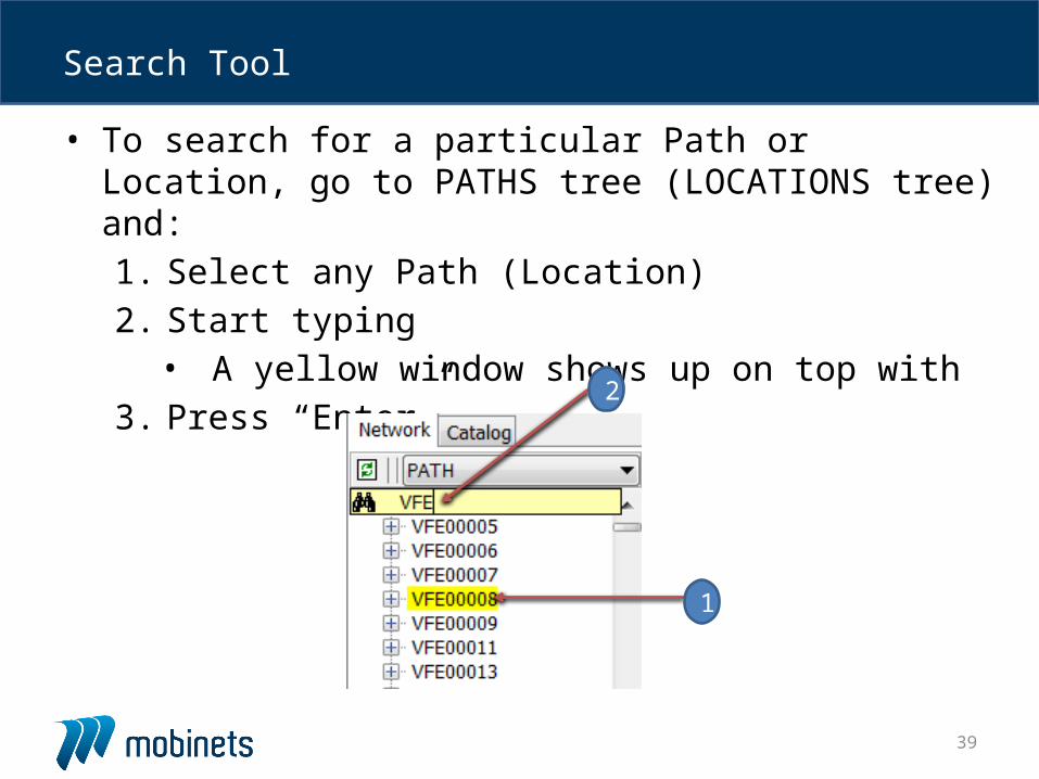
• To search for a particular Path or Location, go to PATHS tree (LOCATIONS tree) and:

1. Select any Path (Location)

2. Start typing• A yellow window shows up on top with

3. Press “Enter”

Search Tool

1

2

40

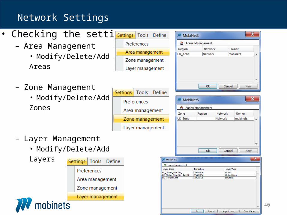
• Checking the settings– Area Management

• Modify/Delete/Add

Areas

– Zone Management• Modify/Delete/Add

Zones

– Layer Management• Modify/Delete/Add

Layers

Network Settings

41

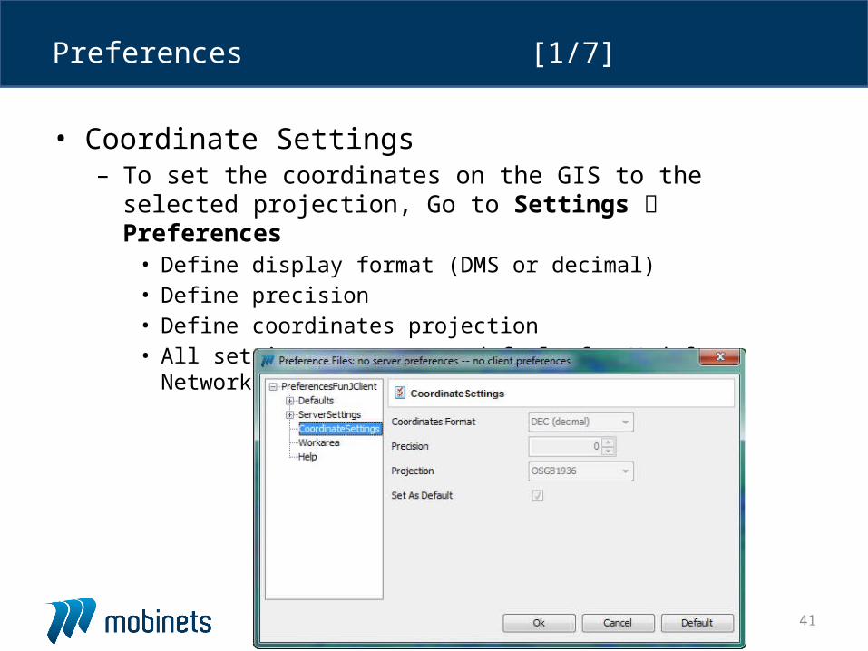
• Coordinate Settings– To set the coordinates on the GIS to the selected projection, Go

to Settings Preferences• Define display format (DMS or decimal)• Define precision• Define coordinates projection• All settings are set as default for Vodafone Network

Preferences [1/7]

42

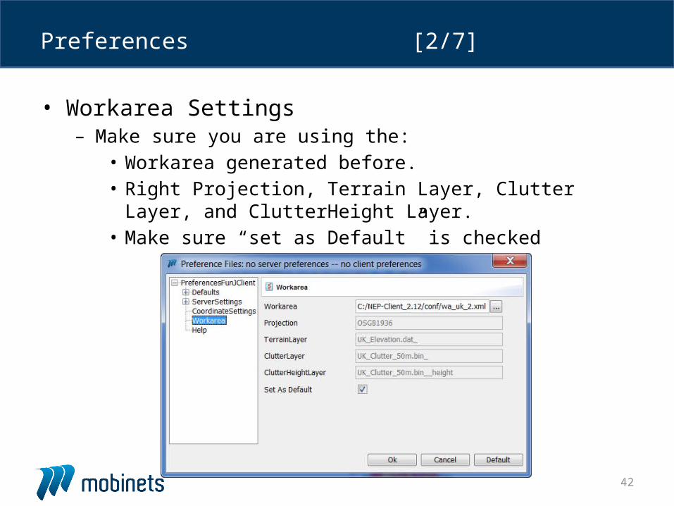
• Workarea Settings– Make sure you are using the:

• Workarea generated before.• Right Projection, Terrain Layer, Clutter Layer, and

ClutterHeight Layer.• Make sure “set as Default” is checked

Preferences [2/7]

43

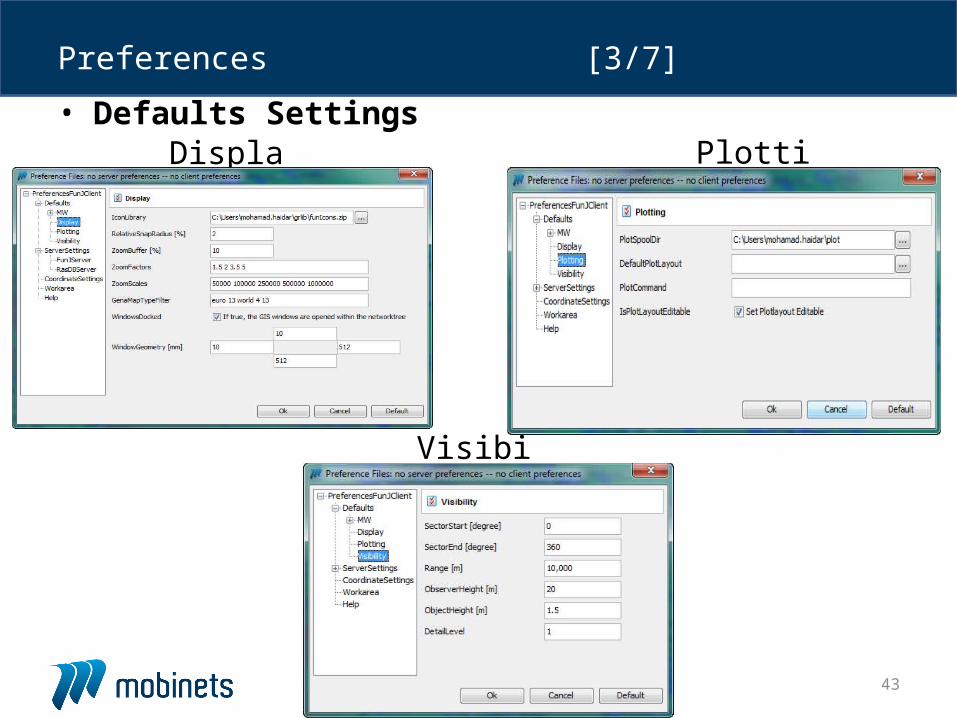
• Defaults Settings

Preferences [3/7]

PlottingDisplay

Visibility

44

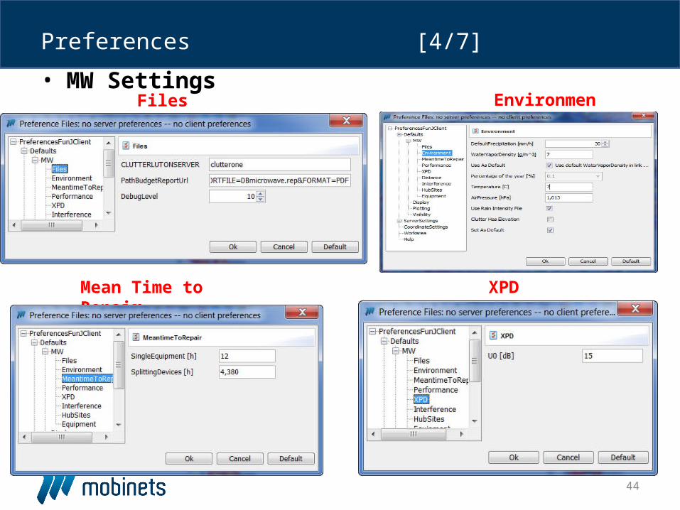
• MW Settings

Preferences [4/7]

Files Environment

Mean Time to Repair XPD

45

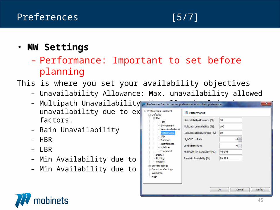
• MW Settings– Performance: Important to set before planning

This is where you set your availability objectives– Unavailability Allowance: Max. unavailability allowed– Multipath Unavailability: Max allowed multipath unavailability due to

external (uncontrolled) factors. – Rain Unavailability– HBR– LBR– Min Availability due to Multipath– Min Availability due to Rain

Preferences [5/7]

46

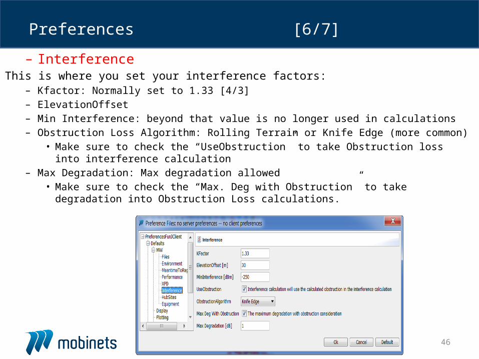
– InterferenceThis is where you set your interference factors:

– Kfactor: Normally set to 1.33 [4/3]– ElevationOffset– Min Interference: beyond that value is no longer used in calculations– Obstruction Loss Algorithm: Rolling Terrain or Knife Edge (more common)

• Make sure to check the “UseObstruction” to take Obstruction loss into interference calculation

– Max Degradation: Max degradation allowed• Make sure to check the “Max. Deg with Obstruction” to take degradation into

Obstruction Loss calculations.

Preferences [6/7]

47

Preferences [7/7]

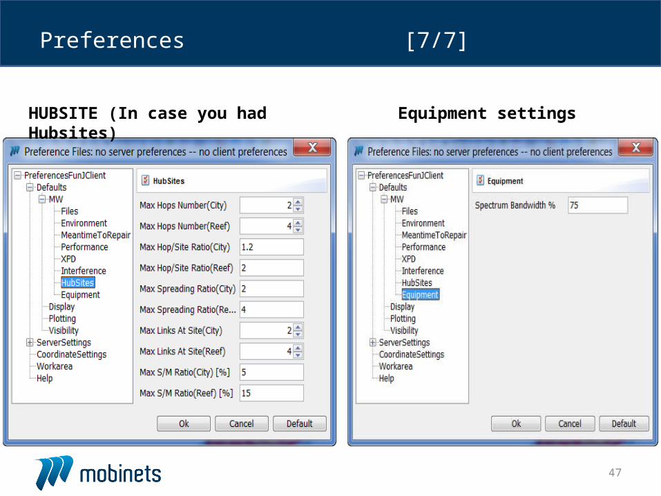
HUBSITE (In case you had Hubsites) Equipment settings

48

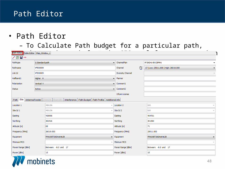
• Path Editor– To Calculate Path budget for a particular path, choose the path from

the GIS or left tree pane then click “Path Editor” tab.

Path Editor

49

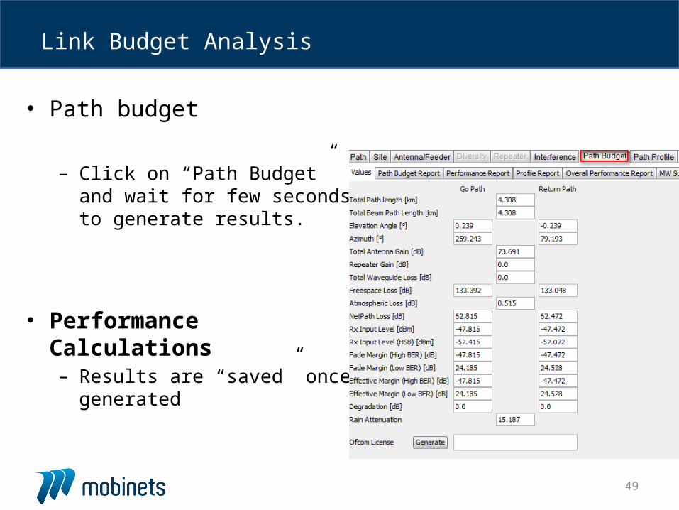
• Path budget

– Click on “Path Budget” and wait for few seconds to generate results.

• Performance Calculations– Results are “saved” once

generated

Link Budget Analysis

50

• Path Budget Report– Summary report of availability objectives due to multipath and

precipitation.

Performance Reports [1/6]

51

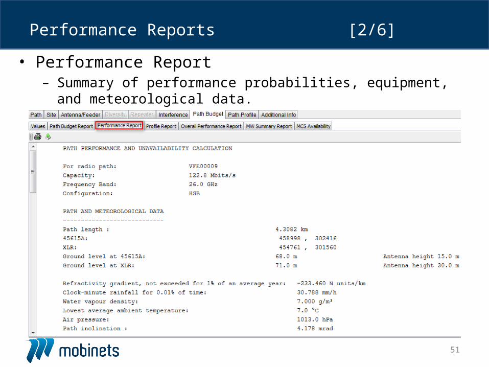
• Performance Report– Summary of performance probabilities, equipment, and

meteorological data.


52

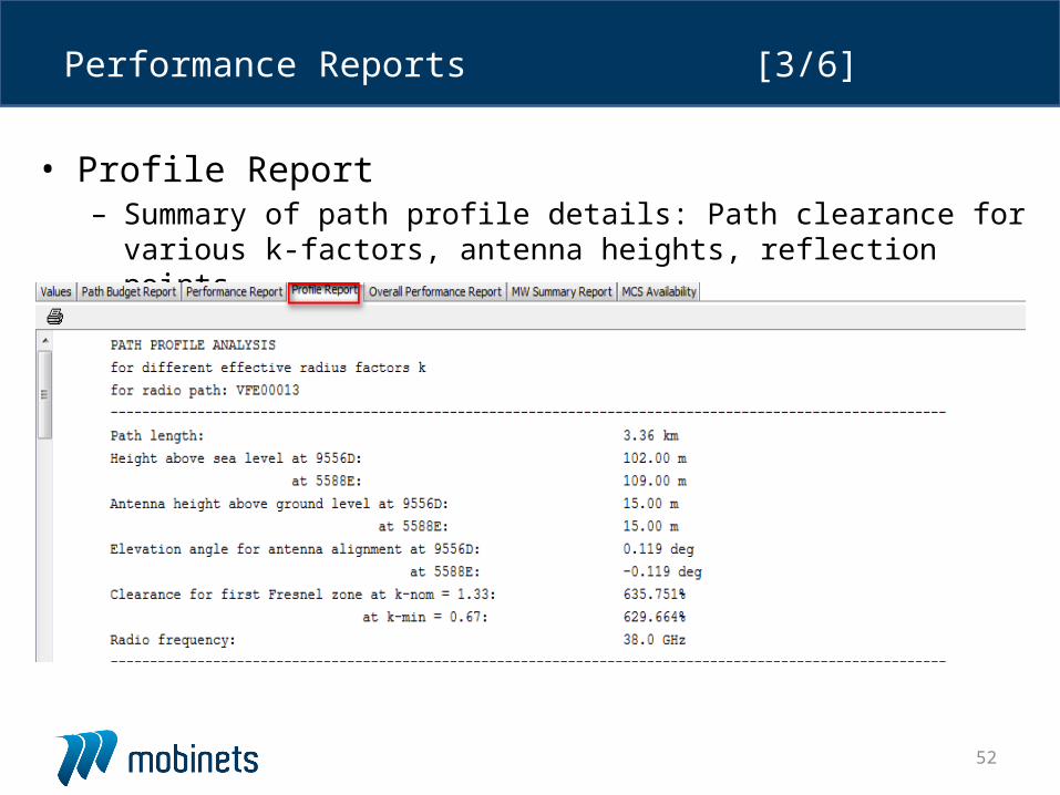
• Profile Report– Summary of path profile details: Path clearance for various k-factors,

antenna heights, reflection points, …


53

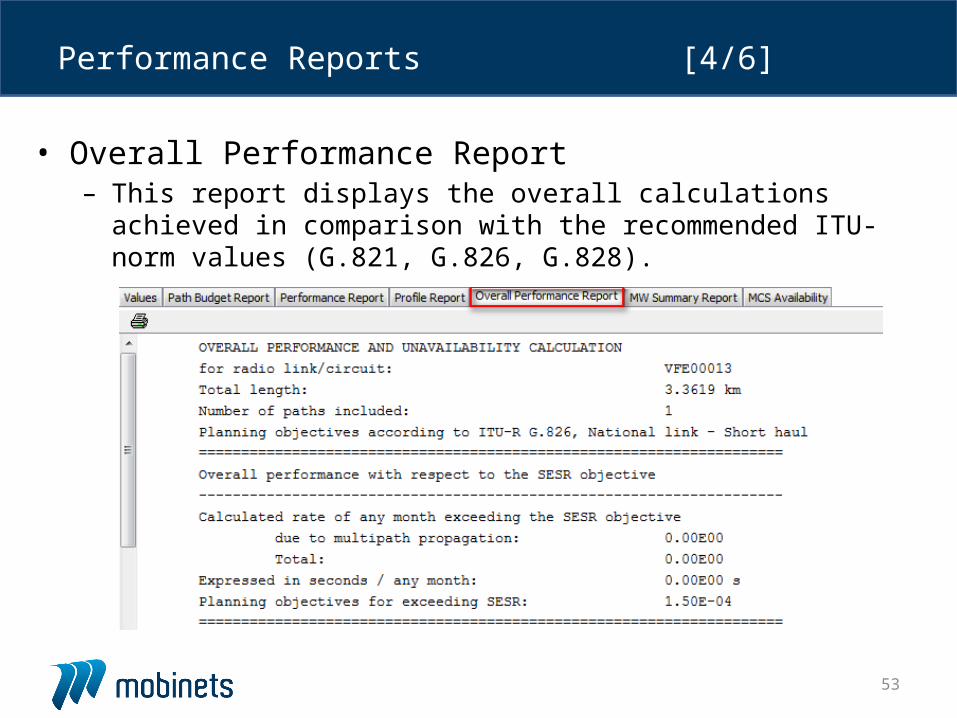
• Overall Performance Report– This report displays the overall calculations achieved in comparison

with the recommended ITU-norm values (G.821, G.826, G.828).


54

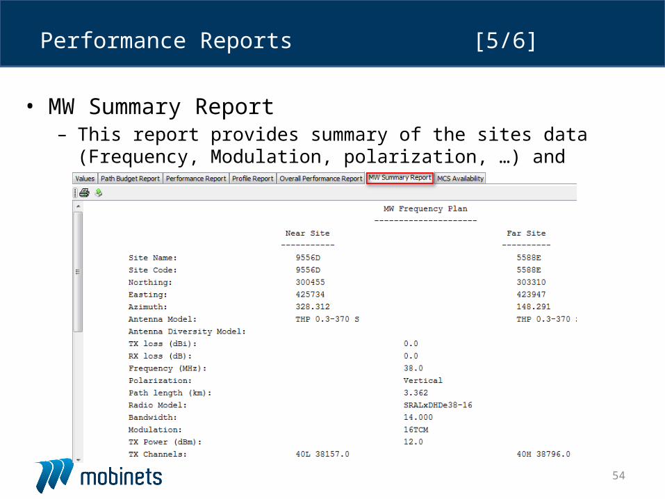
• MW Summary Report– This report provides summary of the sites data (Frequency,

Modulation, polarization, …) and Inventory.


55

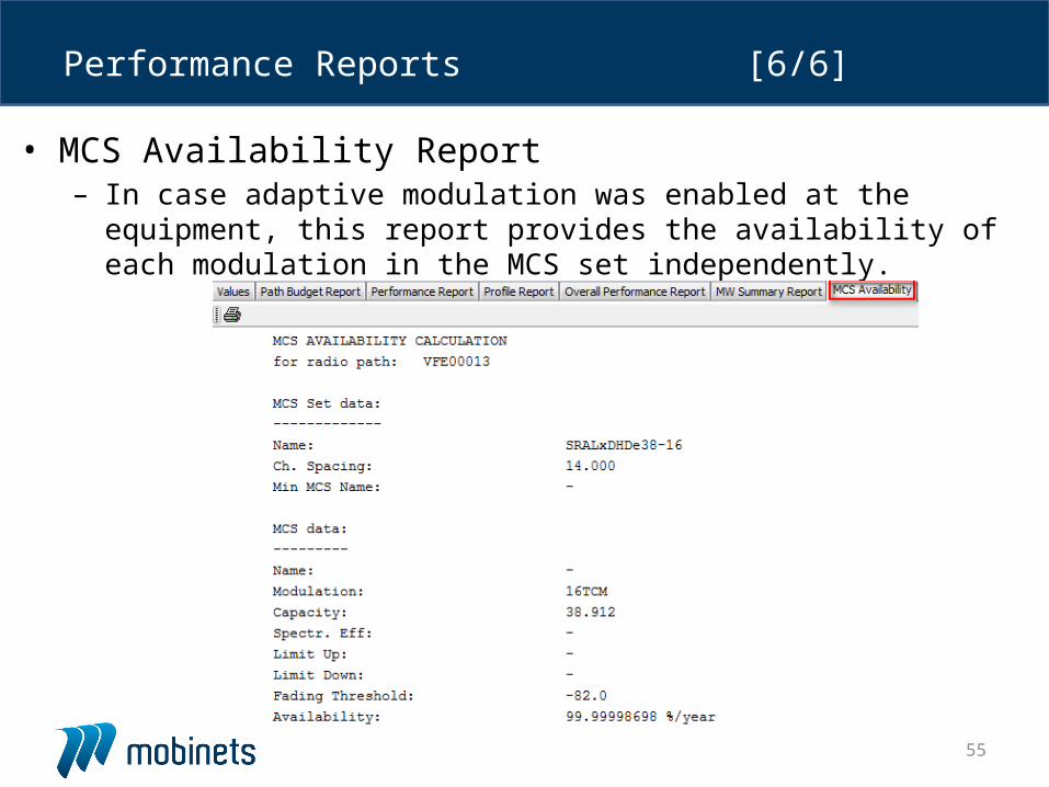
• MCS Availability Report– In case adaptive modulation was enabled at the equipment, this report

provides the availability of each modulation in the MCS set independently.


56

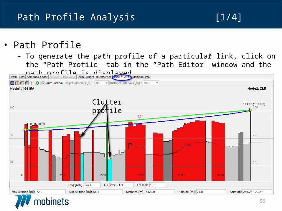
• Path Profile– To generate the path profile of a particular link, click on the “Path Profile” tab in

the “Path Editor” window and the path profile is displayed.

Path Profile Analysis[1/4]

Clutter profile

57

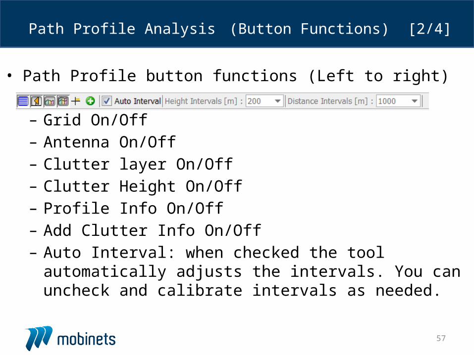
• Path Profile button functions (Left to right)

– Grid On/Off– Antenna On/Off– Clutter layer On/Off– Clutter Height On/Off– Profile Info On/Off– Add Clutter Info On/Off– Auto Interval: when checked the tool automatically adjusts

the intervals. You can uncheck and calibrate intervals as needed.

Path Profile Analysis (Button Functions)[2/4]

58

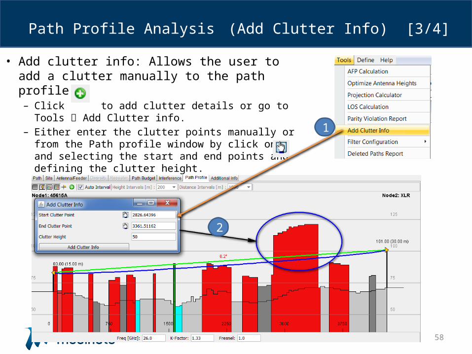
• Add clutter info: Allows the user to add a clutter manually to the path profile.– Click to add clutter details or go to Tools

Add Clutter info.– Either enter the clutter points manually or from

the Path profile window by click on and selecting the start and end points and defining the clutter height.

Path Profile Analysis (Add Clutter Info)[3/4]

1

2

59

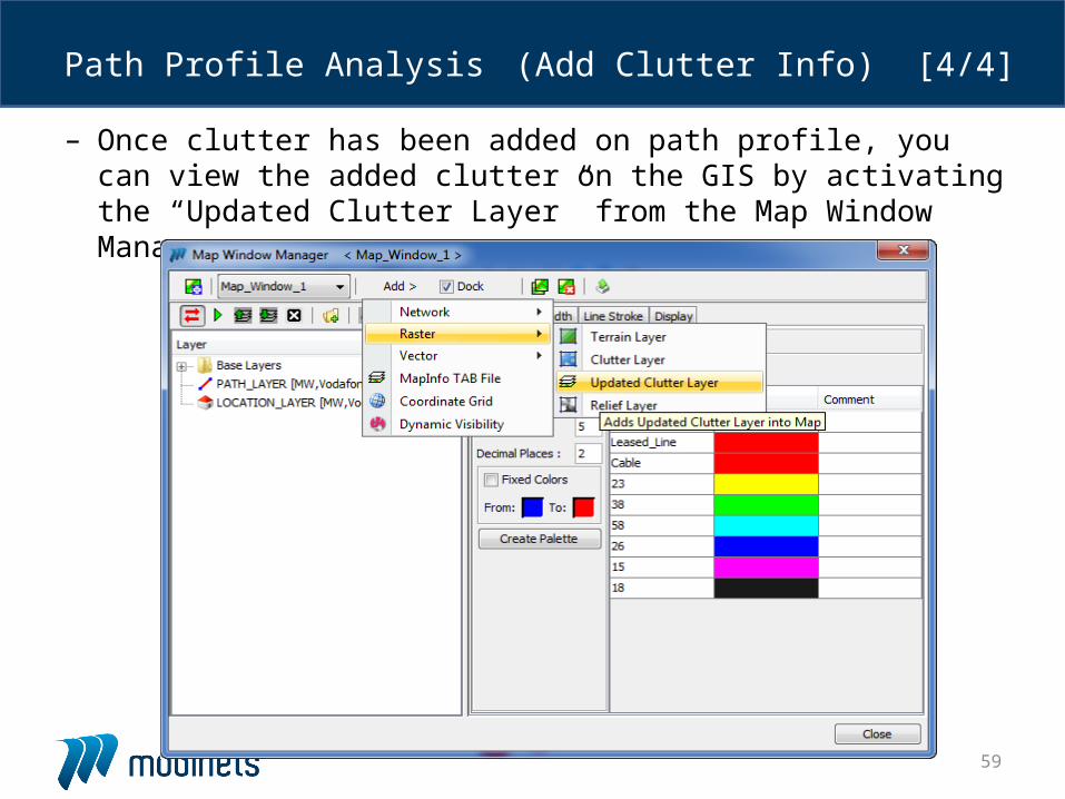
– Once clutter has been added on path profile, you can view the added clutter on the GIS by activating the “Updated Clutter Layer” from the Map Window Manager

Path Profile Analysis (Add Clutter Info)[4/4]

60

• After importing all the catalog/network elements and verifying the settings, we are now able to start applying the features of the tool.

Features

61

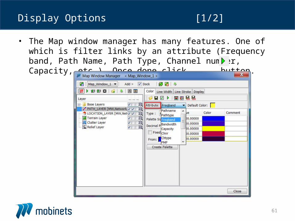
• The Map window manager has many features. One of which is filter links by an attribute (Frequency band, Path Name, Path Type, Channel number, Capacity, etc…). Once done click button.

Display Options [1/2]

62

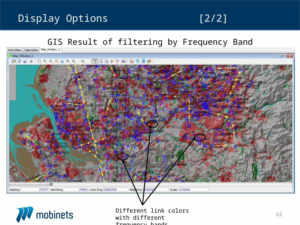
GIS Result of filtering by Frequency Band

Display Options [2/2]

Different link colors with different frequency bands

63

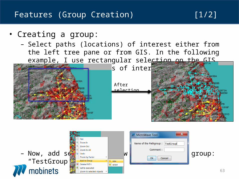
• Creating a group:– Select paths (locations) of interest either from the left tree pane or

from GIS. In the following example, I use rectangular selection on the GIS select the sites/links of interest.

– Now, add selection to new group and name group: “TestGroup”

Features (Group Creation) [1/2]

After selection

64

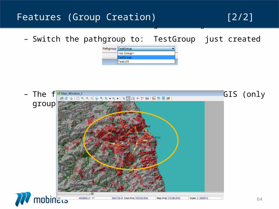
– Switch the pathgroup to: ”TestGroup” just created

– The following should be displayed on the GIS (only group objects)

Features (Group Creation) [2/2]

65

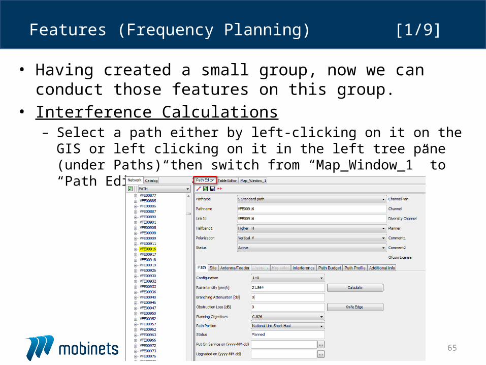
• Having created a small group, now we can conduct those features on this group.

• Interference Calculations– Select a path either by left-clicking on it on the GIS or left clicking on

it in the left tree pane (under Paths) then switch from “Map_Window_1” to “Path Editor”

Features (Frequency Planning) [1/9]

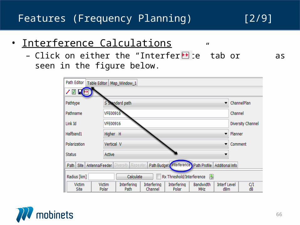
66

• Interference Calculations– Click on either the “Interference” tab or as seen in the figure

below.


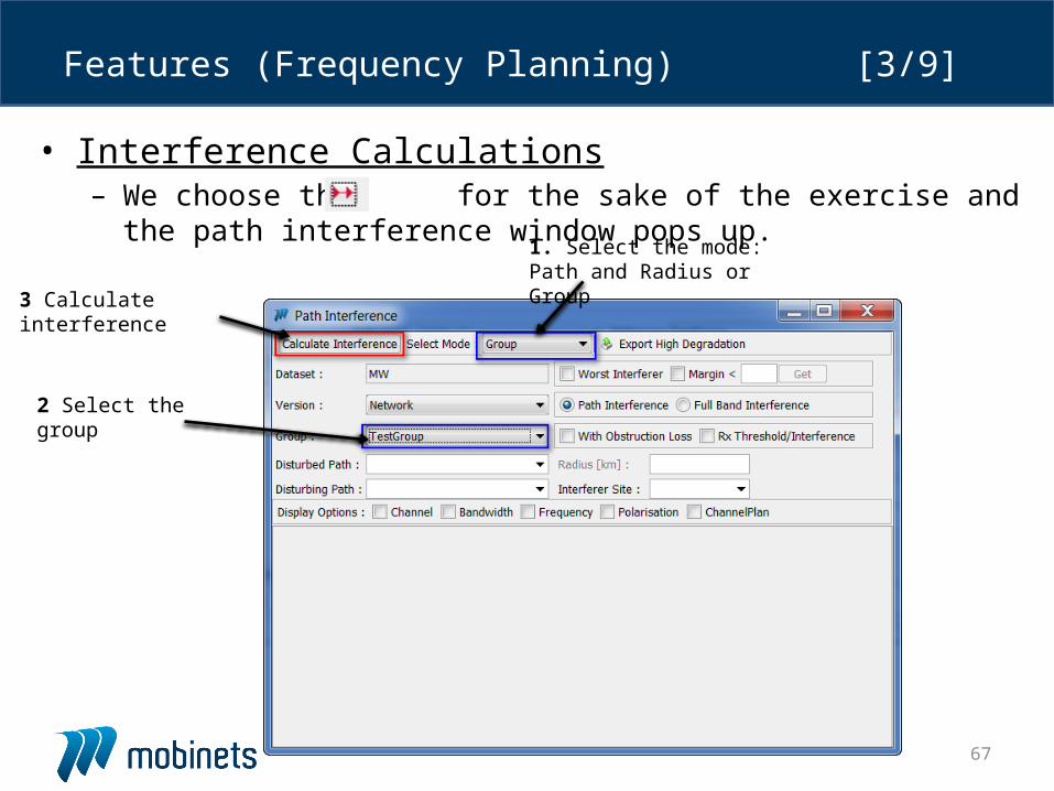
67

• Interference Calculations– We choose the for the sake of the exercise and the path

interference window pops up.


1. Select the mode: Path and Radius or Group

2 Select the group

3 Calculate interference

68

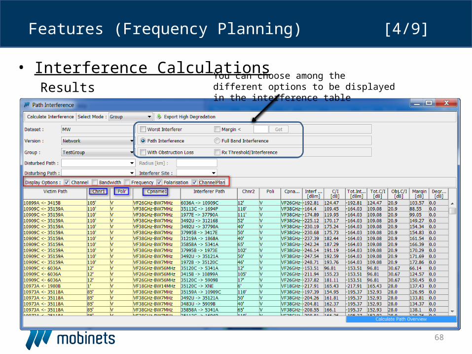
• Interference CalculationsResults


You can choose among the different options to be displayed in the interference table

69

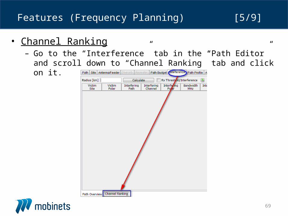
• Channel Ranking– Go to the “Interference” tab in the “Path Editor” and scroll down to

“Channel Ranking” tab and click on it.


70

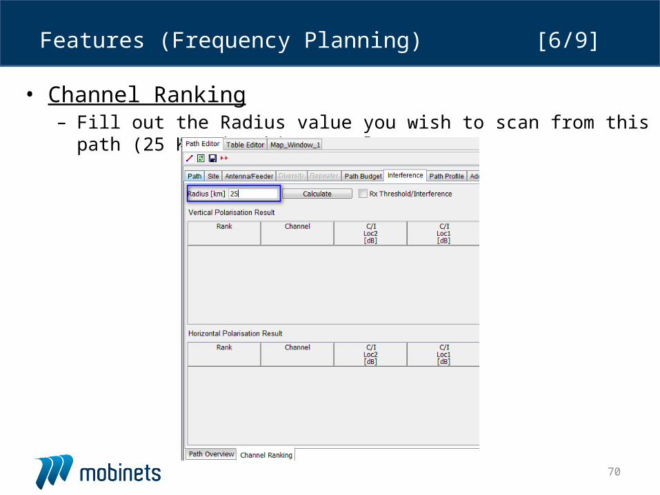
• Channel Ranking– Fill out the Radius value you wish to scan from this path (25 Km) in

this example.


71

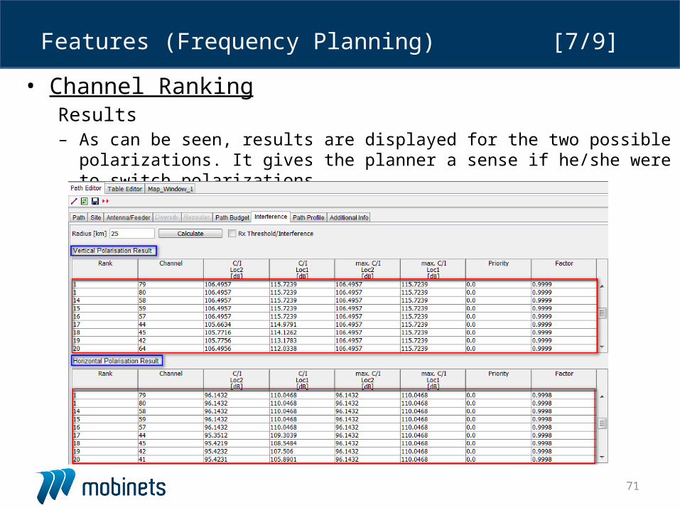
• Channel RankingResults– As can be seen, results are displayed for the two possible polarizations. It

gives the planner a sense if he/she were to switch polarizations.


72

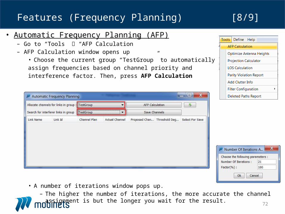
• Automatic Frequency Planning (AFP)– Go to “Tools” “AFP Calculation”– AFP Calculation window opens up

• Choose the current group “TestGroup” to automatically

assign frequencies based on channel priority and

interference factor. Then, press AFP Calculation

• A number of iterations window pops up.– The higher the number of iterations, the more accurate the channel

assignment is but the longer you wait for the result.


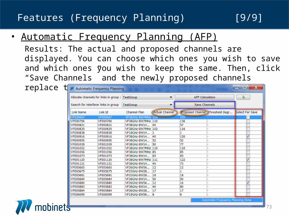
73

• Automatic Frequency Planning (AFP)Results: The actual and proposed channels are displayed. You can choose which ones you wish to save and which ones you wish to keep the same. Then, click “Save Channels” and the newly proposed channels replace the actual ones.


74

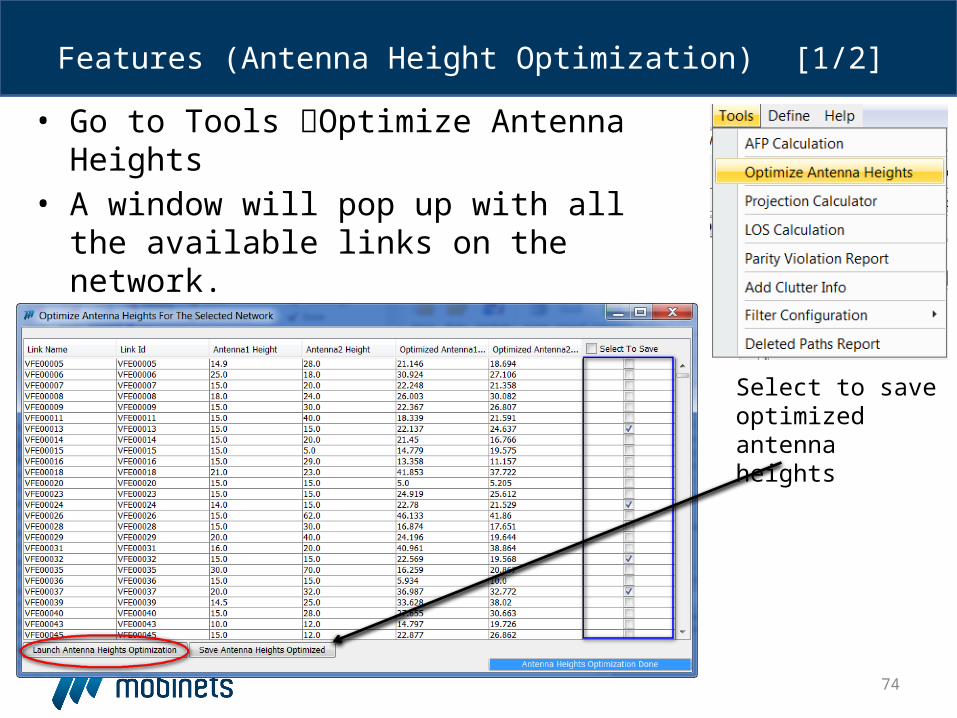
• Go to Tools Optimize Antenna Heights• A window will pop up with all the available

links on the network. • Click “Launch Antenna Height

Optimization”

Features (Antenna Height Optimization) [1/2]

Select to save optimized antenna heights

75

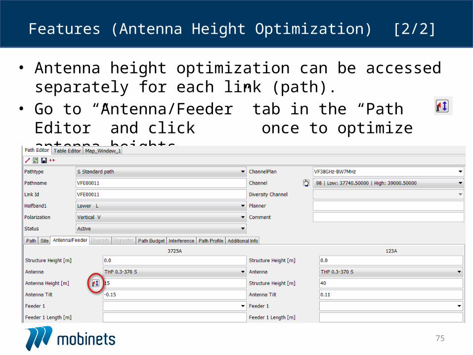
• Antenna height optimization can be accessed separately for each link (path).

• Go to “Antenna/Feeder” tab in the “Path Editor” and click once to optimize antenna heights.

Features (Antenna Height Optimization) [2/2]

76

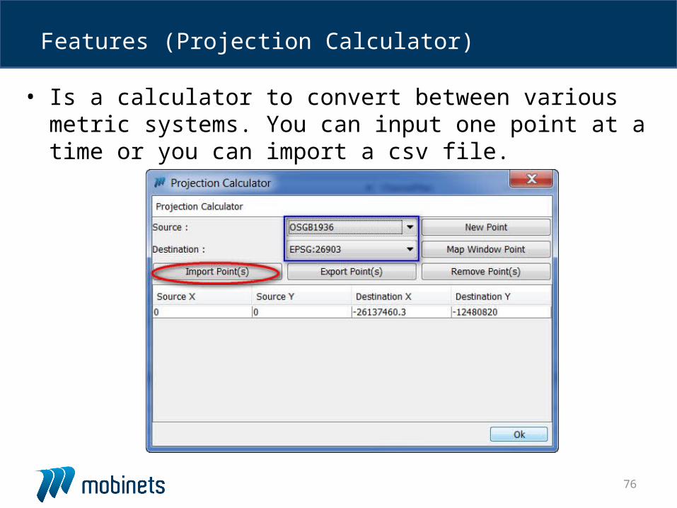
• Is a calculator to convert between various metric systems. You can input one point at a time or you can import a csv file.

Features (Projection Calculator)

77

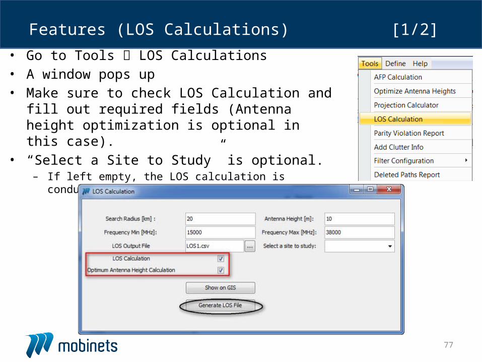
• Go to Tools LOS Calculations• A window pops up• Make sure to check LOS Calculation and fill out

required fields (Antenna height optimization is optional in this case).

• “Select a Site to Study” is optional.– If left empty, the LOS calculation is conducted on the whole

network or group

Features (LOS Calculations) [1/2]

78

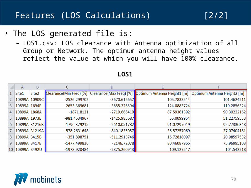
• The LOS generated file is:– LOS1.csv: LOS clearance with Antenna optimization of all Group or

Network. The optimum antenna height values reflect the value at which you will have 100% clearance.

Features (LOS Calculations) [2/2]

LOS1

79

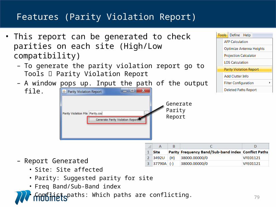
• This report can be generated to check parities on each site (High/Low compatibility)– To generate the parity violation report go to Tools

Parity Violation Report– A window pops up. Input the path of the output file.

– Report Generated• Site: Site affected• Parity: Suggested parity for site• Freq Band/Sub-Band index• Conflict paths: Which paths are conflicting.

Features (Parity Violation Report)

Generate Parity Report

80

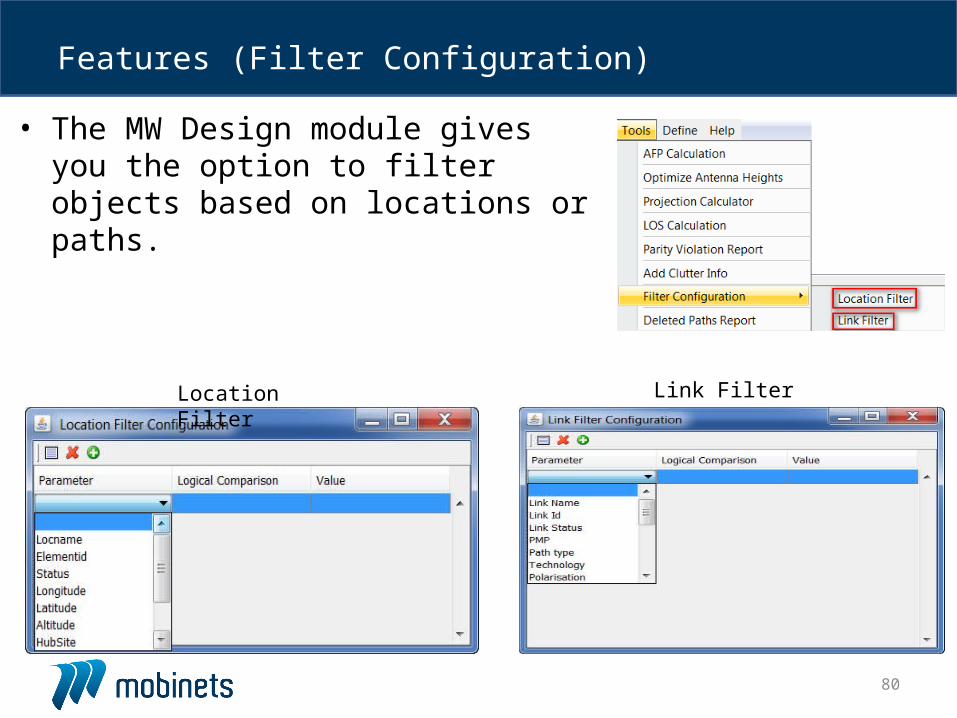
• The MW Design module gives you the option to filter objects based on locations or paths.

Features (Filter Configuration)

Link FilterLocation Filter

81

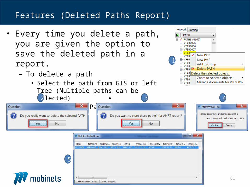
• Every time you delete a path, you are given the option to save the deleted path in a report.– To delete a path

• Select the path from GIS or left Tree (Multiple paths can be selected)

• Click “Delete Path”.

Features (Deleted Paths Report)

1

2 3 4

5

82

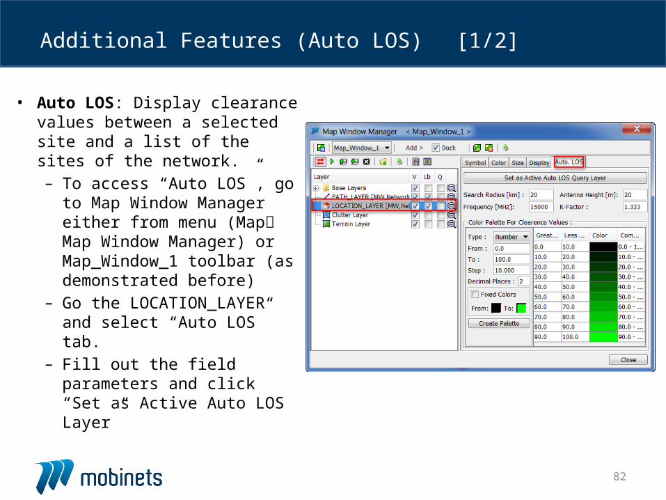
• Auto LOS: Display clearance values between a selected site and a list of the sites of the network.– To access “Auto LOS”, go

to Map Window Manager either from menu (Map Map Window Manager) or Map_Window_1 toolbar (as demonstrated before)

– Go the LOCATION_LAYER and select “Auto LOS” tab.

– Fill out the field parameters and click “Set as Active Auto LOS Layer”

Additional Features (Auto LOS) [1/2]

83

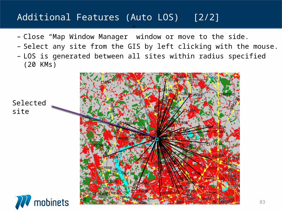
– Close “Map Window Manager” window or move to the side.– Select any site from the GIS by left clicking with the mouse.– LOS is generated between all sites within radius specified (20 KMs)

Additional Features (Auto LOS) [2/2]

Selected site

84

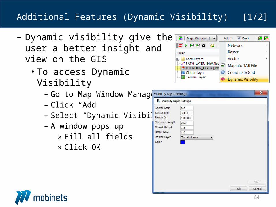
– Dynamic visibility give the user a better insight and view on the GIS

• To access Dynamic Visibility– Go to Map Window Manager– Click “Add”– Select “Dynamic Visibility”– A window pops up

» Fill all fields» Click OK

Additional Features (Dynamic Visibility) [1/2]

85

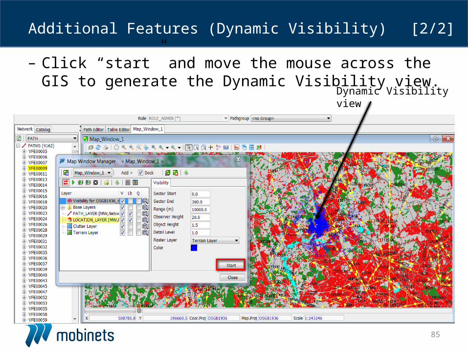
– Click “start” and move the mouse across the GIS to generate the Dynamic Visibility view.

Additional Features (Dynamic Visibility) [2/2]

Dynamic Visibility view

86

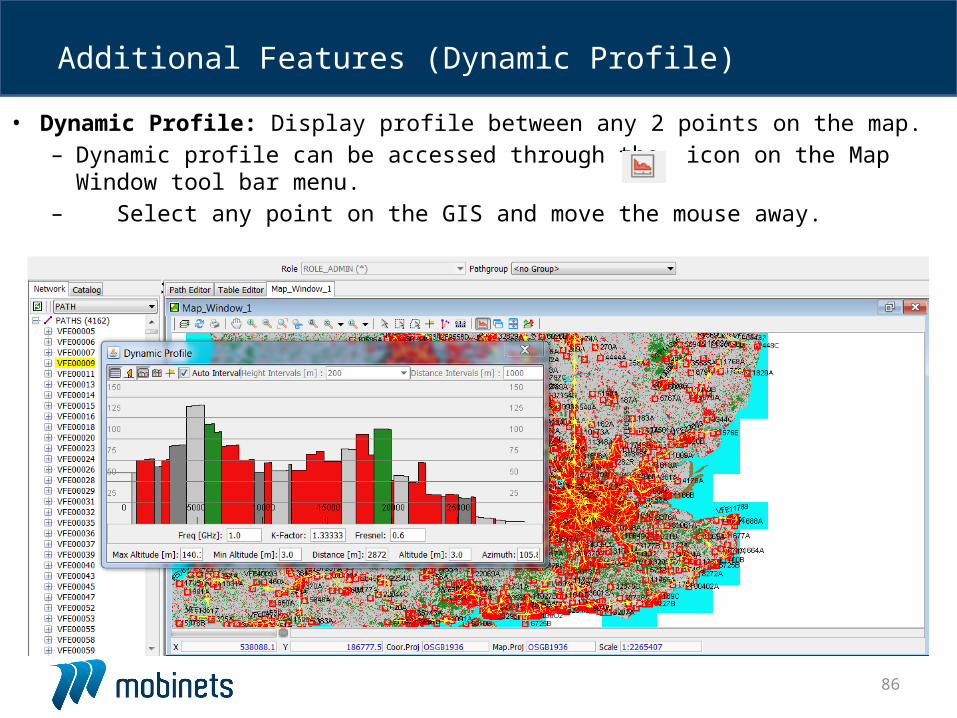
• Dynamic Profile: Display profile between any 2 points on the map.– Dynamic profile can be accessed through the icon on the Map

Window tool bar menu.– Select any point on the GIS and move the mouse away.

Additional Features (Dynamic Profile)

87

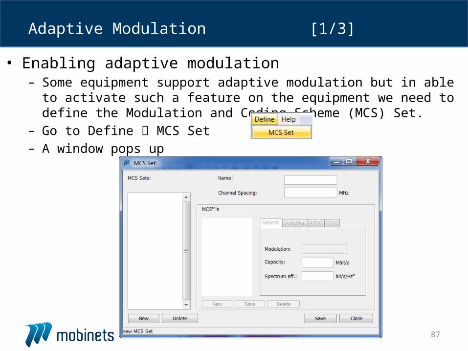
• Enabling adaptive modulation– Some equipment support adaptive modulation but in able to activate

such a feature on the equipment we need to define the Modulation and Coding Scheme (MCS) Set.

– Go to Define MCS Set– A window pops up

Adaptive Modulation [1/3]

88

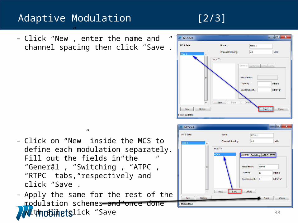
– Click “New”, enter the name and channel spacing then click “Save”.

– Click on “New” inside the MCS to define each modulation separately. Fill out the fields in the “General”, “Switching”, “ATPC”, “RTPC” tabs, respectively and click “Save”.

– Apply the same for the rest of the modulation schemes and once done with all, click “Save”


89

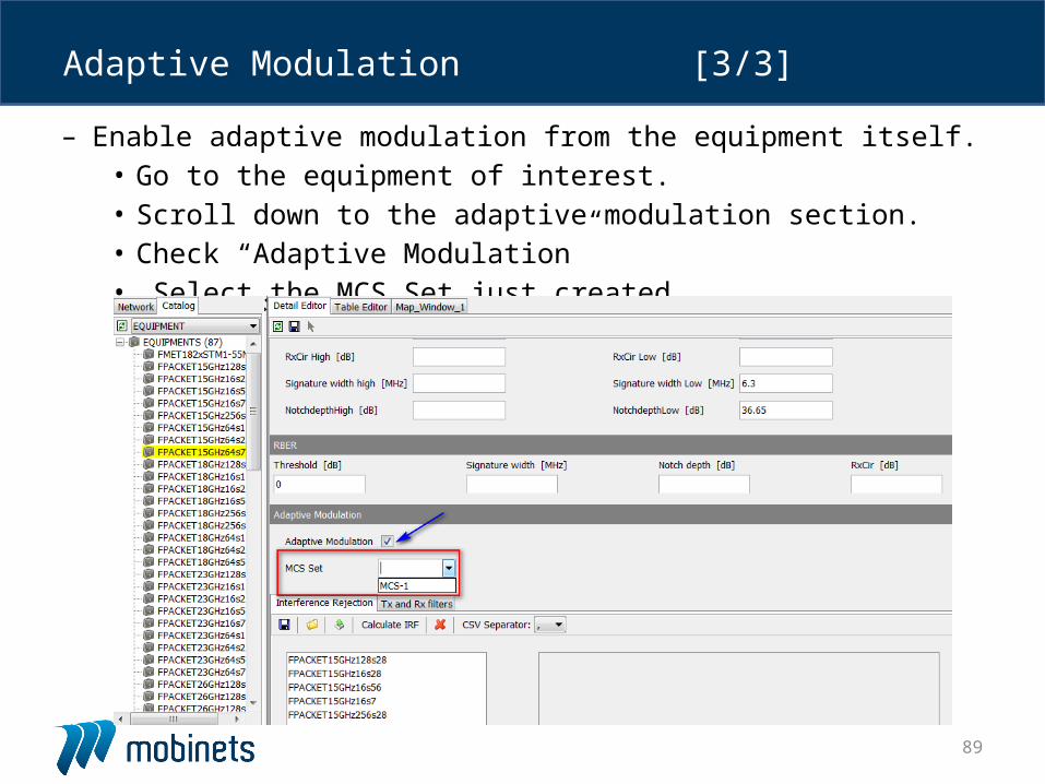
– Enable adaptive modulation from the equipment itself.• Go to the equipment of interest. • Scroll down to the adaptive modulation section.• Check “Adaptive Modulation”• Select the MCS Set just created.


NEP “Microwave Design” Module

Documents

Transcript of NEP “Microwave Design” Module