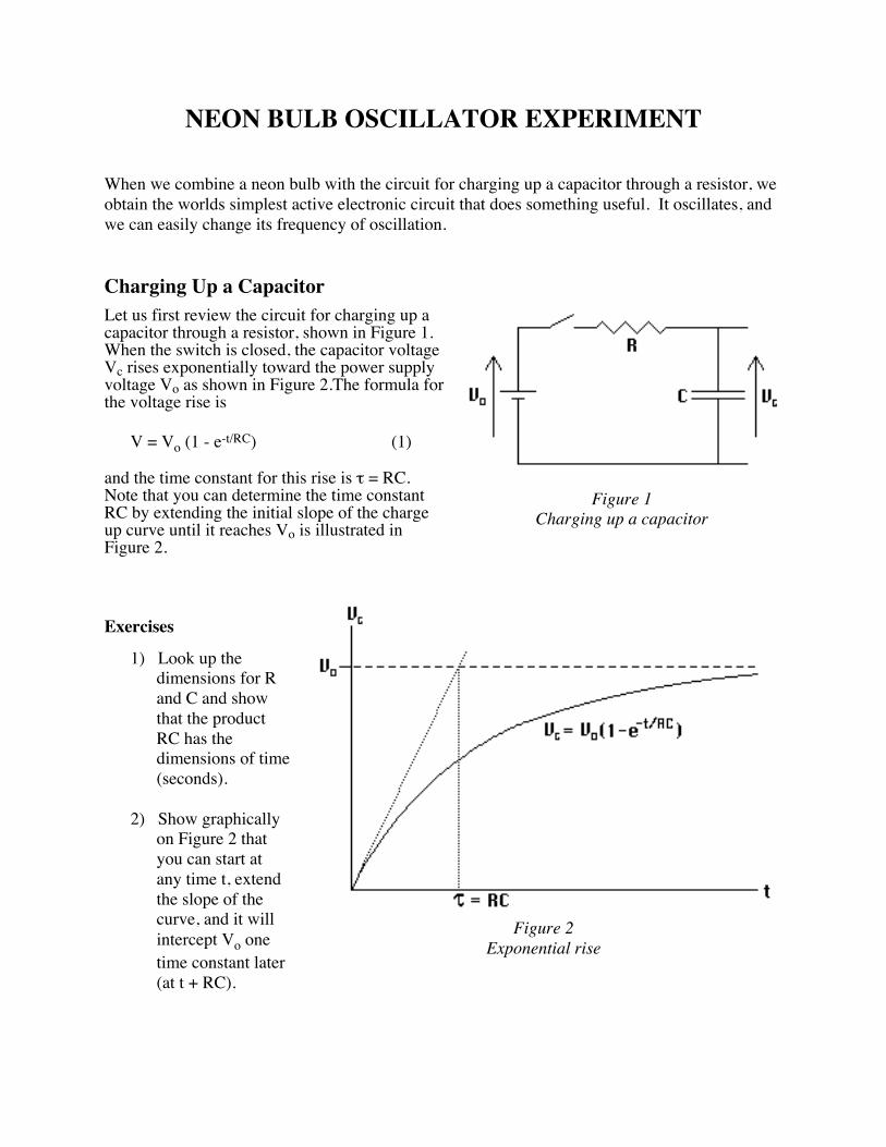
NEON BULB OSCILLATOR EXPERIMENT When we combine a neon bulb with the circuit for charging up a capacitor through a resistor, we obtain the worlds simplest active electronic circuit that does something useful. It oscillates, and we can easily change its frequency of oscillation. Charging Up a Capacitor Let us first review the circuit for charging up a capacitor through a resistor, shown in Figure 1. When the switch is closed, the capacitor voltage Vc rises exponentially toward the power supply voltage Vo as shown in Figure 2.The formula for the voltage rise is V = Vo (1 - e-t/RC) (1) and the time constant for this rise is τ = RC. Note that you can determine the time constant RC by extending the initial slope of the charge up curve until it reaches Vo is illustrated in Figure 2. Exercises

1) Look up the dimensions for R and C and show that the product RC has the dimensions of time (seconds).

2) Show graphically

on Figure 2 that you can start at any time t, extend the slope of the curve, and it will intercept Vo one time constant later (at t + RC).

Figure 1 Charging up a capacitor

Figure 2

Exponential rise

Neon Oscillator

2

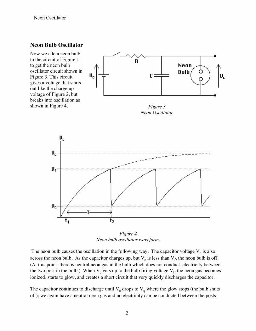
Neon Bulb Oscillator Now we add a neon bulb to the circuit of Figure 1 to get the neon bulb oscillator circuit shown in Figure 3. This circuit gives a voltage that starts out like the charge up voltage of Figure 2, but breaks into oscillation as shown in Figure 4.

The neon bulb causes the oscillation in the following way. The capacitor voltage Vc is also across the neon bulb. As the capacitor charges up, but Vc is less than Vf, the neon bulb is off. (At this point, there is neutral neon gas in the bulb which does not conduct electricity between the two post in the bulb.) When Vc gets up to the bulb firing voltage Vf, the neon gas becomes ionized, starts to glow, and creates a short circuit that very quickly discharges the capacitor. The capacitor continues to discharge until Vc drops to Vq where the glow stops (the bulb shuts off); we again have a neutral neon gas and no electricity can be conducted between the posts

Figure 3 Neon Oscillator

Figure 4 Neon bulb oscillator waveform.

Neon Oscillator

3

inside the bulb. Now the capacitor again charges up through the resistor until Vc reaches Vf and the bulb fires again. This process repeats, giving the wave form shown in Figure 4. Small neon bulbs often have a firing voltage Vf around 100 volts, and a quench voltage Vq around 40 volts. (Some work at lower voltages.) Calculation of the Period of Oscillation To calculate the period T of the oscillation in the neon bulb oscillator, we see from Figure 4 that T = t2 - t1, where t1 is the time when Vc rose up through Vq and t2 is when Vc rose up to the firing voltage Vf. During this time we have the simple charging of a capacitor given by equation 1: Vc = Vo (1 - e-t/RC) (1) Applying Eq. 1 to times t1 (Vc = Vq) and t2 (Vc = Vf) gives Vq = Vo 1 - e-t1/RC (2) Vf = Vo 1 - e-t2/RC (3) Equations (3) and (4) can be rewritten as Voe-t1/RC = Vo - Vq (4) Voe-t2/RC = Vo - Vf (5) Dividing Eq. 4 by Eq. 5 gives

e-t1/RC

e-t2/RC = e t2 - t1 /RC =

Vo - VqVo - Vf (6)

where we used ea/eb = ea-b. Finally taking the logarithm of Eq. 6 gives

T = t2 - t1 = RC Ln

Vo - VqVo - Vf (7)

where Ln is the natural logarithm (Ln ea = a).

Neon Oscillator

4

The Experimental Setup

We could use the experimental setup of Figure 3, putting an oscilloscope across the capacitor and observing Vc directly. This works well with a cathode ray tube (CRT) oscilloscope that can handle the over 100 volts needed to fire the neon bulb. However we will use the computer based oscilloscope MacScope in order to save a record of the wave forms, and MacScope is limited to input voltage in the range of +5 to -5 volts. To use MacScope, we add the voltage divider shown in Figure 5, so that Vc is dropped by a factor of 1000 and can easily be measured by MacScope. The Voltage divider consists of two resistors connected between points A and B of Figure 5. The 107 ohm resistor is so large that very little current flows through it and thus the voltage divider has very little effect on Vc which we wish to measure. MacScope is attached across the 104 ohm resistor, and therefore sees only .1% of the voltage Vc. (Since the same current goes through both resistors, the ratio of the voltages equals the ratio of the resistances.) For safety purposes we put the neon bulb and voltage divider in a single box to reduce the chance of someone putting a finger on one of the high voltage leads. Setting Up the Experiment Since this is one of your first major wiring exercises, we will take you through it in easy steps. Circuit 1 Making sure that the power supply is off, first wire the power supply Vo, the resistance box R, and capacitor box C as shown. The convention in physics and engineering laboratories is that red is positive (+) and black is ground (-). So that you can see what you are doing, use a red wire to go from the red post on the power supply to either of the posts on the resistance box. You might as well use a red wire to go from the other post of the resistance box to the (not low) post of the capacitor box. Finally, use a black wire to go from the "low" post of the capacitor box to the ground (black) post on the power supply. You should now have the circuit shown in figure 6.

Figure 5

Neon oscillator with voltage divider

Figure 6

Basic RC circuit

Neon Oscillator

5

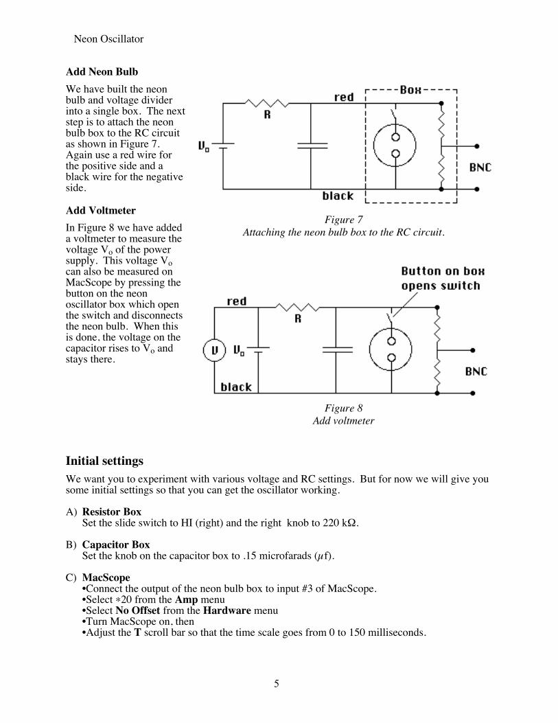
Add Neon Bulb We have built the neon bulb and voltage divider into a single box. The next step is to attach the neon bulb box to the RC circuit as shown in Figure 7. Again use a red wire for the positive side and a black wire for the negative side. Add Voltmeter In Figure 8 we have added a voltmeter to measure the voltage Vo of the power supply. This voltage Vo can also be measured on MacScope by pressing the button on the neon oscillator box which open the switch and disconnects the neon bulb. When this is done, the voltage on the capacitor rises to Vo and stays there. Initial settings We want you to experiment with various voltage and RC settings. But for now we will give you some initial settings so that you can get the oscillator working. A) Resistor Box Set the slide switch to HI (right) and the right knob to 220 kΩ. B) Capacitor Box Set the knob on the capacitor box to .15 microfarads (µf). C) MacScope •Connect the output of the neon bulb box to input #3 of MacScope. •Select *20 from the Amp menu •Select No Offset from the Hardware menu •Turn MacScope on, then •Adjust the T scroll bar so that the time scale goes from 0 to 150 milliseconds.

Figure 7

Attaching the neon bulb box to the RC circuit.

Figure 8

Add voltmeter

Neon Oscillator

6

D) Power Supply Turn the voltage knob all the way down (counter clockwise), and turn the power supply on.

Also turn the standby switch to on. Set the "Volts" - "MA" switch to volts. Now slowly turn up the voltage on the power supply until the neon bulb comes on. The bulb should be flashing. If you turn the voltage up more, it should flash faster. If the voltage is too low, the bulb shuts off, and if too high, it stays on continuously. The interesting range is where it flashes. You should see the saw tooth curve of Figure 9 while the bulb is flashing. Reading MacScope Remember that we have put a 1000 to 1 voltage divider in the circuit, so that each millivolt on the voltage scale actually represents one volt. In addition, in order to get the true voltage values above zero, we have selected No Offset from the Hardware menu as shown in Figure 10. If we had left MacScope on automatic offset, the curve would have been centered and the voltage scale would not have a true zero. (The zero would be at the average of the curve.) Reading Vo The reason for the switch above the neon bulb (shown in Figure 8) is so that we can record the power supply voltage Vo. If we press the button to open the switch, the neon bulb is disconnected from the circuit and the capacitor charges all the way up to Vo. This is read by MacScope. (If you push the button, you see the curve rise to a constant value which is just Vo, corrected by 1000.) Taking data

Figure 9

Saw tooth curve on MacScope

Figure 10 Selecting No Offset and Negative Trigger Slope

Neon Oscillator

7

We can use the trigger capability of MacScope to grab both Vo and the oscillating curve in one data file. Set MacScope on negative trigger as shown in Figure 10, hold down the switch button so that the voltage Vo goes to MacScope, and adjust the MacScope trigger button just below Vo as shown in Figure 11. Now set MacScope on Trigger (as in Figure 12), and start it. When you release the switch, current flows through the bulb and the voltage drops. The dropping voltage activates the negative trigger and MacScope starts recording data.

Figure 11

Neon Oscillator

8

In the resulting curve is shown in Figure 12. The pretrigger data (t < 0) shows Vo, while the post trigger data t > 0 shows the oscillation. Analyzing MacScope Data Once we have the MacScope data, there are a number of ways to get information from it. In Figure 13, we used the cursor to measure the height of Vo. We do this by dragging a rectangle whose height is equal to Vo and reading the height in the rectangle that appears while we are dragging. The answer is 164 volts (remember the factor 1000).

Figure 12

The MacScope trigger captures the curve just when we release the disconnect switch, and the neon bulb is back in the ciorcuit. The pre trigger data (t < 0) shows the power supply voltage Vo.

Figure 13

Using the cursor to measure Vo.

Neon Oscillator

9

A more accurate way to measure Vo is to use the editor as shown in Figure 14, where we have selected data just before and after t = 0. Here we see that Vo is 159.3 volts. The accuracy of this number depends upon how well your MacScope was calibrated.

In Figure 15 we have used the cursor to measure the period of the oscillation and got 45.6 milliseconds or a frequency of about 22 hz. We could also use the editor and numerical data as we did in Figure 14.

Figure 14

Using the numerical values to measure Vo.

Figure 15

Using the cursor to measure the period. The amplitude of the wave was increased using the "V" scroll bar at the top of the

control panel.

Neon Oscillator

10

Finally, we note that the time constant RC = 220 x 103 Ω * .15 x 10-6 F = 33 x 10-3 sec or 33 ms. We drew a rectangle 33 ms wide going up to Vo as shown in Figure 16. Drawing the diagonal we see that it accurately represents the initial slope as expected by theory. (The capacitor is on exponential rise to Vo.) The Experiment The neon bulb oscillator is enormously flexible. By choosing different values of R and C, you can easily have the period range from the order of a millisecond to many seconds. Changing Vo changes the shape of the wave form and also changes the period. What you should do is try different values of R and C to get a broad range of periods. Also change Vo to get different shaped wave forms from the pointed saw tooth waves (Vo >> Vf) to round top waves (when Vo is just above Vf). Record the results as MacScope files for later analysis. As an instructive exercise, adjust Vo down until it is just above Vf, so that the bulb barely fires. Then the curve looks very much like Figure 2 for the charge up of a capacitor. Save this wave form as a MacScope file, and use this as experimental data to (a) verify that the initial slope intercepts Vo at one time constant RC down the T axis, and b) carry out exercise 2 with this data. (Take your MacScope file of this curve home, bring up this curve on your own Macintosh, and adjust the amplification and the time base so that the curve nicely fills the screen. Then do an imagewriter screen dump and do your exercises on the screen dump.)

Figure 16

Demonstration that the initial slope of the curve intersects Vo at one time constant RC.

Neon Oscillator

11

Computer Analysis of RC Circuits

Earlier we considered the analytic solution, first of the discharge, then of the charging up, of a capacitor through a resistor. The results: V = Vo e-t/RC (Discharge) (1) V = Vo (1-e-t/RC) (Charge up) (2) were fairly easy to obtain for the discharge, but took us a whole page when we added one more term to handle charging up. Analytic solutions have the advantage of giving general results that cover a wide range of parameters, but it becomes difficult to obtain analytic solutions when the problem becomes just a bit more complicated. In contrast, computer solutions can be generalized with very little additional work. In this section we will first discuss a computer program for capacitor discharge, show how it is easily modified for charge up, and then modify it some more to describe the neon bulb oscillator. Discharge To analyze the capacitor discharge, we go back to Kirchoff's law and set the sum of the voltage rises equal to zero: Vc - VR = 0

qC - iR = 0

(3)

We now have one equation and two variables q and i. The other equation is obtained by noting that i is the rate charge is leaving the capacitor:

i = - dq

dt (4)

Equations 3 and 4 will be the basis of our computer program. Equation 4 is a differential equation (it involves dq/dt), and therefore needs special handling. First we "undo" the calculus by writing dq = - idt (5) where we think of dt as a small but finite time interval.

Neon Oscillator

12

The quantity dq is the change in the charge q during the time dt. If we call qold the amount of charge in the capacitor before dt, and qnew the charge after dt, then qnew and qold can be related by the command LET qnew = qold + dq (6) Using equation 5 for dq, our command for calculating qnew becomes LET qnew = qold - i *dt (7)

At this point equation 7 is very close to being a command in the computer language BASIC. In BASIC, we can think of each variable, like q, i, and dt as the name on a mailbox (the kind you see in a post office). Inside the mailbox goes a number that is the current value of the variable. When given a LET statement, the computer goes to the right hand side, looks up the values of the variables, performs the indicated operations, and then stores the result in the mailbox whose name is one the left hand side. In the case of equation 7, the computer will look in the mailboxs labeld q, i, and dt, multiply the numerical values of i and dt together, and subtract that product from the numerical value found in mailbox labled q. The computer then goes to the mailbox labled q and replaces the contents with the value just calculated. An automatic consequence of this procedure for a LET statement is that the computer must use old values in order to calculate the right hand side, and the result automatically becomes the new value on the left hand side. Thus it is not necessary to write down the subscripts new and old; that happens automatically and Eq. 7, written as a BASIC statement becomes LET q = q - i *dt (8) Once the computer calculates a new value of q, it needs a new value of i, which it can get from Eq.3 i = q/RC or as a let statement LET i = q/(R*C) (9) Now that the computer has the new value of i from Eq. 9, it goes back and calculates the next new value of q. This process is repeated over and over again in a calculational loop indicated schematically in Eq. 10;

Neon Oscillator

13

(10)

Neon Oscillator

14

The Computer Program Equation (10) is not a complete program for we have to tell the computer what values of R, C, and dt to use; what initial value of q should be used, and how to plot the results as we go along. Figure 1 is a complete program for discharging a 10-8 farad capacitor through a 106 ohm resistor. Let us go through each piece of this program to see how it works. In the first block we tell the computer the experimental constants. Aside from giving the values for R and C. we are saying that we had a 150 volt power supply (V0 = 150). In the initial conditions we are saying that the capacitor is initially fully charged (Vc = Vo, q = CVo at time T = 0). From Ohms law we get VR = iR or i = VR /R From the definition of capacitancewe get q = CVc or Vc = q/C Kirchoff's Law gives Vc - VR = 0, Vc = VR = iR, or i = Vc/R The charge flows out of the capacitor to create the current i, thus i = dq/dt or dq = - i*dt qnew = qold + dq = qold - i*dt The Time Step

Figure 1

Simple program for capacitor Discharge

Neon Oscillator

15

The point of the computer calculation is to break the discharge into small time steps dt, calculate the amount of charge dq that leaves the capacitor during that time step (we had dq = - i*dt ), and then subtract that charge from what remains in the capacitor (qnew = qold + dq). In order to get an accurate calculation, the time step dt must be sufficiently small that the current i does not change much during the time step (otherwise we would not know what value of i to use in dq = i*dt). From our earlier discussion we know that the capacitor voltage drops to 1/e (1/2.7) of its original value in one time constant T = RC. This is a big step, too big for our small time step dt. What we have done in the time step section is choose one tenth of a time constant for our time step. This is still a big time step, but it gives fairly accurate results. (The current i does not change too much in one tenth of a time constant.) The Discharge Loop The discharge loop is bracketed by the commands DO WHILE T < 3*R*C - - - - LET i = Vc/R LET q = q - i*dt LET Vc = q/C LET T = T + dt PRINT "T";TAB(40*Vc/V0);T - - - - LOOP What the computer does when it meets such a loop command is to repeat what is inside the loop while the condition (T < 3*R*C) is met. In this case the loop will be repeated while T is less than 3 time constants (30 steps). Inside the loop we have changed things a little bit from Eq. 10. We put the equation for i first, and replaced q/C by VC since the capacitor voltage VC is what we can observe directly: LET i = Vc/R [was LET i = q/(R*C) ] The next line is our command LET qnew = qold - i*dt with the subscripts new and old dropped. Then we use the definitions of capacitance C = q/Vc to calculate the new capacitor voltage Vc from the new q LET Vc = q/C

Neon Oscillator

16

Then we update our clock with the command. LET Tnew = Told + dt since an amount of time dt elapses every time we go around the loop.

Neon Oscillator

17

Typewriter Plotting It does not do any good to have the computer calculate all these new values for q and Vc is we cannot see the results. In the last, rather peculiar looking line inside the discharge loop, we PRINT out the results using BASIC's version of standard typewriter operations. In the command PRINT "T";TAB(40*Vc/V0);T three printing steps are involved (separated by semicolons). In the first step the computer prints the letter T; this gives us the vertical axis of T's seen in the output of Fig. 1. Next the computer tabs over a number of spaces proportional to Vc. (If Vc = Vo, we go over 40 spaces; if Vc = V0/2, we go over 20 spaces etc.) Finally we print out the numerical value of the time T so that we can see in the plot how much time has elapsed for each step. There are much more precise ways to plot the capacitor voltage Vc, but none give us the time scale as easily. We will discuss other plotting techniques later, typewriter plotting will do for now. Exercise 1 Directly on the output of Figure 1, show that that curve has a time constant of about .01 seconds. Do this by showing that any tangent line intersects the axis one time constant later. A More Accurate Program An inherent weakness of the program in Figure 1 is that we used a relatively large time step dt = RC/10. The computer is perfectly capable of calculating with a much smaller time step and repeating the discharge loop many more times. But if we used a smaller time step in Figure 1, and printed out the value of Vc every time, we would have to look through a very long plot before we see much of a discharge of the capacitor. In order to use a short time step but not print out too much, we have in figure 2 added the following lines to the discharge loop. FOR N = 1 to 10 ---- calculate for ---- one time step dt NEXT N now print out the results

Neon Oscillator

18

In this so called FOR NEXT statement the computer calculates new values of Vc for 10 time steps before printing out the results. However we used a time step dt that was ten times shorter than the time step in Figure 1, (.01 RC instead of .1RC), so that we got essentially the same results. There is a slight difference because the calculation in Figure 2 is more accurate.

Neon Oscillator

19

Exercise 2 Type in the program of Figure 2 and run it to see that you get the same results. Then cut the time step to one thousandths of a time constant and adjust the FOR-NEXT loop so that you get essentially the same results.

Figure 2

Capacitor Discharge with a Shorter Time Step. This is the same calculation as in Figure 1, except that we used a time step 10 times shorter, but then used the FOR NEXT loop to do 10 calculations

of Vc before printing the results.

Neon Oscillator

20

Capacitor Charge Up In our analytic solutions there was a big change when we went from capacitor discharge to capacitor charge up. In a computer program, the change is very small. In Figure 3 we show the circuit, program, and output for the charging of a capacitor. The program of Figure 3 is identical to the program of Figure 2 except for two lines in the charge up loop. In Figure 1, Kirchoff's law required that Vc - VR = Vc - iR = 0 giving the command LET i = Vc/R In Figure 3, Kirchoff's law requires that V0 - VR - Vc = V0 - iR - Vc = 0 giving the new command LET i = V0/R - Vc/R The only other change is that current is now flowing into the capacitor in Figure 3 where it flowed out of C in the discharge of Figures 1 & 2. Thus the sign of i is now reversed in the command LET q = q + i*dt In the output of Figure 3, we see our standard capacitor charge up curve.

Neon Oscillator

21

Exercise 3 Use graphical methods on the output curve of Figure 3 to show that the time constant for this capacitor charge up is approximately.01 seconds. Show what your graphical methods were.

Figure 3

Capacitor chargeup

Neon Oscillator

22

Neon Bulb Oscillator One modification of our charge up program of Figure 3 and we end up with a program for the neon bulb oscillator shown in Figure 4. To effectively add a neon bulb to our circuit, we went to the calculational loop and watched the capacitor voltage Vc. When Vc got up over the bulb firing voltage Vf, we immediately dropped Vc back to the bulb shutoff or quench voltage Vq, and reduced the charge q in the capacitor to the value CVq that it should have at this voltage. We then let the capacitor charge up again, discharge, etc., and get the typical neon bulb oscillator voltage shown. Lab Exercises For several of your experimental neon oscillator results in this weeks lab, use the program of Figure 4 to compare the prediction of this program with your experimental results. This requires in each case using your experimental values for R, C, V0, Vf, and Vq. Then compare the

Figure 4 Neon Bulb Oscillator. We can effectively add a neon bulb to our charge up program by monitoring the capacitor voltage Vc in the

charge up loop. When Vc gets up to the bulb firing voltage Vf, we drop Vc back to the bulb shutoff voltage Vq and reduce the charge q to CVq.

Neon Oscillator

23

shape and timing of the output of your program with the curve you stored as a MacScope file. (Use screen dumps of both to make the comparison). Comment on the results.

Neon Oscillator

24