NEAR EAST UNVERSITY

Faculty of Engineering

Department of Computer Engineering

I

FACE RECOGNITION SYSTEM

Graduation Project Com-400

Student: Azzam Qumsieh

Supervisor: Assoc. Prof. Dr. Adnan Khashman

Nicosia - 2002

ACKNOWLEDGEMENTS

"I would like to thank my supervisor Assoc Prof Dr. Adnan Khashman for his

invaluable advice and the limitless help he had shown.

Also, I thank the Near East University in general and specially Prof Dr Şenol

Bektaş.

And, I would like to dedicate this work to my family who have supported and

encourage me to reach a higher degree of education. Father and Mother, I gave you all

my respects and love for all your support and for believing in me. Also I would give my

thanks and love to my brother and all my sisters spicily to abeer and her husband nader

for all the support they gave me.

Finally, I would also like to thank all my friends for their advice and support. "

ABSTRACT

People in computer vision and pattern recognition have been working on automatic

recognition of human faces for the last 20 years. Given a digital image of a person's

, face, face recognition software matches it against a database of other images. If any of

the stored images matches closely enough, the system reports the sighting to its owner,

and so the efficientway to perform this is to use an ArtificialIntelligence system.

The aim of this project is to discus the development of the face recognition system.

For this purpose the state of the art of the face recognition is given. However, many

approaches to face recognition involving many applications and there eigenfaces to

solve the face recognition system problems is given too. For example, the project

contain a description of a face recognition system by dynamic link matching which

shows a good capabilityto solve the invariant object recognition problem.

A better approach is to recognize the face in unsupervised manner using neural

network architecture. We collect typical faces from each individual, project them onto

the eigenspace and neural networks learn how to classify them with the new face

descriptor as input.

ii

TABLE OF CONTENTS

ACKOWLEDGEMNET ABSTRACT TABLE OF CONTENTS INTRODUCTION CHAPTER ONE: INTRODUCTION TO

FACE RECOGNITION SYSTEMS

i ii iii V

1

1 2234 46 89

10

l. 1 Overview1:;. History and Mathematical Framework

1 .2. 1 The Typical Representational Framework1.2.2 Dealing with the Curse of Dimensionality

1 .3 Person Identification via Face Recognition1.3.l History of Face Recognition1 .3 .2 Current State of the Art1.3.3 Commercial Systems and Applications

1.4 SummaryCHAPTER TWO: APPROACHES TO

FACE RECOGNITION 1010111213131515151616171819 20

2.1 Overview2.2 Face Recognition for Smart Environments2.3 Wearable Recognition Systems2.4 Future of Face Recognition Technology2.5 Geometrical Features2.6 Eigenfaces2.7 Template Matching2.8 Graph Matching2.9 Neural Network Approaches2.1O The ORL Database2.11 Related Works2.12 Karhunen-Loeve Transform2.13 Convolutional Network2. 14 SummaryCHAPTER THREE: AN AUTOMATIC SYSTEM FOR

DETECTION, RECOGNITION AND CODING OF FACES

20212223252830

3.1 Overview3.2 Detection and Alignment3.3 Recognition and coding3.4 Eigenfaces Demo3.5 Modular Eigenspaces: Detection, Coding and Recognition3 .6 Detection Performance on a Large Database3.7 Modular Image Reconstruction

ll l

3.8 Modular Recognition3.9 Summary

3133

CHAPTER FOUR: FACE RECOGNITION BY DYNAMIC LINK MATCHING

34

4. 1 Overview4.2 Architecture and Dynamics4.3 Blob Formation4.4 Blob Mobilization4.5 Layer Interaction and Synchronization4.6 Link Dynamics4.'Y Attention Dynamics4.8 Recognition Dynamics4.9 Bidirectional Connection4.1 O Blob Alignment in Model Domain4.11 Maximum Versus Sum Neurons4.12 Experiments

4. 12.1 Data Base4.12.2 Technical Aspects4. 12.3 Results

4.12 Discussion4.13 SummaryCHAPTER FIVE: PRINCIPAL COMPONENT

ANALYSIS AND NEURAL NETWORK

343640 424345464950505051515153555758

5.1 Overview5.2 Face Detection

5.2.1 Face Model Resize5 .2.2 Edge Removal5.2.3 Illumination Normalization

5.3 Face Recognition5 .3 .1 Eigenspace Representation5.3.2 Neural Network5.3.3 Training Set5.3.4 Normalize Training Set

5.4 SummaryCONCLUSION REFERENCES

585960 60 60 60 616667 686869 71

IV

lN'rRODUC'rlON

Twenty years ago the problem of face recognition was considered among the

hardest in Artificial Intelligence (AI) and computer vision. Surprisingly, however, over

the last decade there have been a series of successes that have made the general person

identification enterprise appear not only technically feasible but also economically

practical.

Face recognition in general and the recognition of moving people in natural

soenes in particular, require a set of visual tasks to be performed robustly.

These include:

(1) Acquisition: the detection and tracking of face-like image patches in

a dynamic scene.

(2) Normalisation: the segmentation, alignment and normalisation of the

face images.

(3) Recognition: the representation and modelling of face images as

identities, and the association of novel face images with known

models.

The project discus the ways that perform these tasks, and it also gives some

results and researches for Face Recognition by several methods. The project consists of

introduction, 5 chapters and conclusion.

Chapter one presents the history of Face Recognition and why it is important,

with some~methodsshows how we can perform the recognition.

Chapter tow presents the approaches to Face Recognition which include many

applications that performs to Face Recognition.

Chapter three describes an .Automaticsystem for detection, recognition and

coding of faces with an eigenfaces demo to show how it works.

V

Chapter four describes a Face Recognition System by Dynamic Link Matching,

the most encouraging aspect of the system is its evident capability to solve the invariant

object recognition problem.

Chapter five describes the principal component analysis and neural network for

Face Recognition, the training set of neural network are described. The efficiency of its

application is analyzed.

Finally conclusion presents the obtained important results and contributions in

the project.

The objectives of this project are:

• Describe the important of face recognition and show where we can use it.

• Show the approaches to face recognition and discus its applications.

• Maintain an automatic system for detection and recognition by given an

eigenfaces demo to show how its work.

• Maintain a face recognition by dynamic link matching and see if it is has

the capability to solve the invariant object recognition problem.

• Use neural network to recognize the human face and analyze its

application to see if its efficiency or not.

Vl

CHAPTER ONE

INTRODUCTION TO

FACE RECOGNITION SYSTEM

1.1 Overview Given the requirement for determining people's identity, the obvious question is

what technology is best suited to supply this information? There are many different

identification technologies available, many of which have been in wide-spread

commercial use for years. The most common person verification and identification

methods today are Password/PIN (Personal Identification Number) systems, and Token" systems (such as your driver's license). Because such systems have trouble with forgery,

theft, and lapses in users' memory, there has developed considerable interest in

biometric identification systems, which use pattern recognition techniques to identify

people using their physiological characteristics. Fingerprints are a classic example of a

biometric; newer technologies include retina and iris recognition.While appropriate for bank transactions and entry into secure areas, such

technologies have the disadvantage that they are intrusive both physically and socially.

They require the user to position their body relative to the sensor, and then pause for a

second to 'declare' themselves. This 'pause and declare' interaction is unlikely to change

because of the fine-grain spatial sensing required. Moreover, there is a 'onıcle-like'.,.· -

aspect to the interaction: since people can't recognize other people using this soft of

data, these types of identification do not have a place in normal human interactions and

social structures.While the 'pause and present' interaction and the oracle-like perception are

useful in high-security applications (they make the systems look more accurate), they

are exactly the opposite of what is required when building a store that recognizes its

best customers, or an information kiosk that remembers you, or a house that knows the

people who live there. Face recognition from video and voice recognition have a natural

place in these next-generation smart environments -- they are unobtrusive (able to

recognize at a distance without requiring a 'pause and present' interaction), are usually

passive (do not require generating special electro-magnetic illumination), do not restrict

user movement, and are now both low-power and inexpensive. Perhaps most important,

1

however, is that humans identify other people by their face and voice, therefore are

likely to be comfortable with systems that use face and voice recognition.

1.2 History and Mathematical Framework Twenty years ago the problem of face recognition was considered among the

hardest in Artificial Intelligence (AI) and computer vision [1]. Surprisingly, however,

over the last decade there have been a series of successes that have made the general

person identification enterprise appear not only technically feasible but also

economically practical.The apparent tractability of face recognition problem combined with the dream

of smart environments has produced a huge surge of interest from both funding agencies

and from researchers themselves. It has also spawned several thriving commercial

enterprises. There are now several companies that sell commercial face recognition

software that is capable of high-accuracy recognition with databases of over 1,000

people.These early successes came from the combination of well-established pattern

recognition techniques with a fairly sophisticated understanding of the image generation

process. In addition, researchers realized that they could capitalize on regularities that

are peculiar to people, for instance, that human skin colors lie on a one-dimensional

manifold (with color variation primarily due to melanin concentration), and that human

facial geometry is limited and essentially 2-D when people are looking toward the

camera. Today, researchers are working on relaxing some of the constraints of existing

face recognition algorithms to achieve robustness under changes in lighting, aging,

rotation-in-depth, expression and appearance (beard, glasses, makeup) -- problems that

have partial solution at the moment.

1.2.1 The Typical Representational Framework

The dominant representational approach that has evolved is descriptive rather

than generative. Training images are used to characterize the range of 2-D appearances

of objects to be recognized. Although initially very simple modeling methods were

used, the dominant method of characterizing appearance has fairly quickly become

estimation of the probability density function (PDF) of the image data for the target

class.

2

For instance, given several examples of a target class Q in a low-dimensional

representation of the image data, it is straightforward to model the probability

distribution functionp(x/Q) of its image-level features x as a simple parametric function

(e.g., a mixture of Gaussians), thus obtaining a low-dimensional, computationally

efficient appearance model for the target class.

Once the PDF of the target class has been learned, we can use Bayes' rule to

perform maximum a posteriori (MAP) detection and recognition. The result is typically

a very simple, neural-net-like representation of the target class's appearance, which can

be used to detect occurrences of the class, to compactly describe its appearance, and to

efficiently compare different examples from the same class. Indeed, this

representational framework is so efficient that some of the current face recognition

methods can process video data at 30 frames per second, and several can compare an

incoming face to a database of thousands of people in under one second -- and all on a

standard PC!

1.2.2 Dealing with the Curse of Dimensionality

To obtain an 'appearance-based' representation, one must first transform the

image into a low-dimensional coordinate system that preserves the general perceptual

quality of the target object's image. This transformation is necessary in order to address

the 'curse of dimensionality' [2]. The raw image data has so many degrees of freedom

that it would require millions of examples to learn the range of appearances directly.

Typical methods of dimensionality reduction include Karhıınen-Loeve transform (KLT)

(also called Principal Components Analysis (PCA)) or the Ritz approximation (also

called 'example-based representation'). Other dimensionality reduction methods are

sometimes also employed, including sparse filter representations (e.g., Gabor Jets,

Wavelet transforms), feature histograms, independent components analysis, and so

forth.These methods have in common the property that they allow efficient

characterization of a low-dimensional subspace with the overall space of raw image

measurements. Once a low-dimensional representation of the target class (face, eye,

hand, etc.) has been obtained, standard statistical parameter estimation methods can be

used to learn the range of appearance that the target exhibits in the new, low­

dimensional coordinate system. Because of the lower dimensionality, relatively few

3

examples are required to obtain a useful estimate of either the PDF or the inter-class

discriminant function.

An important variation on this methodology is discriminative models, which

attempt to model the differences between classes rather than the classes themselves.

Such models can often be learned more efficiently and accurately than when directly

modeling the PDF. A simple linear example of such a difference feature is the Fisher

discriminant. One can also employ discriminant classifiers such as Support Vector

Machines (SVM) which attempt to maximize the margin between classes.

1.3 Person Identification via Face RecognitionThe current literature on face recognition contains thousands of references, most

dating from the last few years. For an exhaustive survey of face analysis techniques the

reader is referred to Chellappa et al. [3], and for current research the reader is referred to

the IEEE Conferences on Automatic Face and Gesture Recognition.

Research on face recognition goes back to the earliest days of AI and computer

vision. Rather than attempting to produce an exhaustive historical account, our focus

will be on the early efforts that had the greatest impact on the community (as measured

by, e.g., citations), and those few current systems that are in wide-spread use or have

received extensive testing.

1.3.1 History ofFace Recognition

The subject of face recognition is as old as computer vision, both because of the

practical importance of the topic and theoretical interest from cognitive scientists.

Despite the fact that other methods of identification (such as fingerprints, or iris scans)

can be more accurate, face recognition has always remains a major focus of research

because of its non-invasive nature and because it is people's primary method of person

identification.

Perhaps the most famous early example of a face recognition system is due to

Kohonen , who demonstrated that a simple neural net could perform face recognition

for aligned and normalized face images. The type of network he employed computed a

face description by approximating the eigenvectors of the face image's autocorrelation

matrix; these eigenvectors are now known as 'eigenfaces.'

4

Kohonen's system was not a practical success, however, because of the need for precise

alignment and normalization. In following years many researchers tried face recognition

schemes based on edges, inter-feature distances, and other neural net approaches. While

several were successful on small databases of aligned images, none successfully

addressed the more realistic problem of large databases where the location and scale of

the face is unknown.

Kirby and Sirovich (1989) [4] later introduced an algebraic manipulation which

made it easy to directly calculate the eigenfaces, and showed that fewer than 100 were

required to accurately code carefully aligned and normalized face images. Turk and

Pentland (1991) [51] then demonstrated that the residual error when coding using the

eigenfaces could be used both to detect faces in cluttered natural imagery, and to

determine the precise location and scale of faces in an image. They then demonstrated

that by coupling this method for detecting and localizing faces with the eigenface

recognition method, one could achieve reliable, real-time recognition of faces in a

minimally constrained environment. This demonstration that simple, real-time pattern

recognition techniques could be combined to create a useful system sparked an

explosion of interest in the topic of face recognition.

A face, bunch graph lscreated from 70 hıcemodels to obta.1ngener~ repreşerıtatlon ofthe face

Given an image the face 1.matched to the face bı.ııchgraph to find ttıe flduclalpolnts

An image graph ls createdusing elastlc graphmatching and çornpared todata.bse of faces forrecognition

5

Figure 1.1 Face Recognition using Elastic Graph Matching

1.3.2 Current State of the Art

By 1993 there were several algorithms claiming to have accurate performance in

minimally constrained environments. To better understand the potential of these

algorithms, DARPA and the Army Research Laboratory established the FERET

program with the goals of both evaluating their performance and encouraging advances

in the technology.There are three algorithms that have demonstrated the highest level of

recognition accuracy on large databases (1196 people or more) under double-blind

testing conditions. These are the algorithms from University of Southern California

(USC) , University of Maryland (UMD) , and the MIT Media Lab . All of these are

participants in the FERET program. Only two of these algorithms, from USC and MIT,

are capable of both minimally constrained detection and recognition; the others require

approximate eye locations to operate. A fourth algorithm that was an early contender,

developed at Rockefeller University , dropped from testing to form a commercial

enterprise. The MIT and USC algorithms have also become the basis for commercial

systems.The MIT, Rockefeller, and UMD algorithms all use a version of the eigenface

transform followed by discriminative modeling. The UMD algorithm uses a linear

discriminant, while the MIT system, seen in Figure 1.3, employs a quadratic

discriminant. The Rockefeller system, seen in Figure 1.2, uses a sparse version of the

eigenface transform, followed by a discriminative neural network. The USC system,

seen in Figure 1.1, in contrast, uses a very different approach. It begins by computing

Gabor 'jets' from the image, and then does a 'flexible template' comparison between

image descriptions using a graph-matching algorithm.

The FERET database testing employs faces with variable position, scale, and

lighting in a manner consistent with mugshot or driver's license photography. On

databases of under 200 people and images taken under similar conditions, all four

algorithms produce nearly perfect performance. Interestingly, even simple correlation

matching can sometimes achieve similar accuracy for databases of only 200 people .

This is strong evidence that any new algorithm should be tested with at databases of at

least 200 individuals, and should achieve performance over 95% on mugshot-like

images before it can be considered potentially competitive.

In the larger FERET testing (with 1166 or more images), the performance of the

four algorithms is similar enough that it is difficult or impossible to make meaningful

6

distinctions between them (especially if adjustments for date of testing, etc., are made).

On frontal images taken the same day, typical first-choice recognition performance is

95% accuracy. For images taken with a different camera and lighting, typical

performance drops to 80% accuracy. And for images taken one year later, the typical

accuracy is approximately 50%. Note that even 50% accuracy is 600 times chance

performance.

Smaff set of featuresfa, Reoeplive fields that are matohed to the looal featuresd the faöe

mouth i•ine oheekbon

Figure 1.2 Face Recognition using Local Analysis

7

a.ea tıc» mı.gıt ıa eııpıeNCıı,,cı a& aIIIQaf a>n1>iıatiQnof ihtl, •İj1JftfırıC~

4.Gwn a test ffi391 it is appıuııimıııtııdas a cnıminatbn of ~bı.cos. Adslance masure is uHd., çr;:ımpa19 thesim~ bahı,9Qn twolınıgııs. p

S(p,

Appearance mod

1. 1'fwo dı.tasitts ,Oı ud .Qı:; are oblainild•one by computin9 iftt~rsonatd'ıffıııwıms (by matching two views d es;ı, indııtiıal il tıı• dı.1&.t) and tother by computing extmperscıı-1diknnceıS {by matching diffoNf'ltjıd,'guals in lht dı1ıHtl ~pee

2. Two Hts d egınfıcits Ut gıneıı.t«iby parfDmıi"9 PCAonMeh cu

3.Simiarlty sa>l9 t»~ two i~ isdtrlYOCI by ak:ubıling s = P(.QıtA).WMl9 A i.S lM diffe,encebııtwNtı a patof m-,.s. 1woiınıgn are Qlll9nrinedto be the sam9 indivclualil S > 0.5

Discriminative mod

Figure 1.3 Face Recognition using Eigenfaces

1.3.3 Commercial Systems and Applications

Currently, several face-recognition products are commercially available.

Algorithms developed by the top contenders of the FERET competition are the basis of

some of the available systems; others were developed outside of the FERET testing

framework. While it is extremely difficult to judge, three systems -- Visionics, Viisage,

and Miros -- seem to be the current market leaders in face recognition.

Visionics' Facelt face recognition software is based on the Local Feature

Analysis algorithm developed at Rockefeller University. Facelt is now being

8

incorporated into a Close Circuit Television (CCTV) anti-crime system called

'Mandrake' in United Kingdom. This system searches for known criminals in video

acquired from 144 CCTV camera locations. When a match occurs a security officer in

the control room is notified.

Viisage, another leading face-recognition company, uses the eigenface-based

recognition algorithm developed at the MIT Media Laboratory. Their system is used in

conjunction with identification cards (e.g., driver's licenses and similar government ID

cards) in many US states and several developing nations.

Miros uses neural network technology for their TrueFace face recognition

software. TrueFace is used by Mr. Payroll for their check cashing system, and has been

deployed at casinos and similar sites in many US states.

1.4 SummaryFace recognition technology has come a long way in the last twenty years.

Today, machines are able to automatically verify identity information for secure

transactions, for surveillance and security tasks, and for access control to buildings etc.

These applications usually work in controlled environments and recognition algorithms

can take advantage of the environmental constraints to obtain high recognition

accuracy.

9

CHAPTER TWO

APPROACHES TO

FACE RECOGNITION

2.1 Overview

Face recognition systems are no longer limited to identity verification and

surveillance tasks. Growing numbers of applications are starting to use face-recognition

as the initial step towards interpreting human actions, intention, and behavior, as a

central part of next-generation smart environments. Many of the actions and behaviors

humans display can only be interpreted if you also know the person's identity, and the

identity of the people around them. Examples are a valued repeat customer entering a

store, or behavior monitoring in an eldercare or childcare facility, and command-and­

control interfaces in a military or industrial setting. In each of these applications identity

information is crucial in order to provide machines with the background knowledge

needed to interpret measurements and observations of human actions.

2.2 Face Recognition for Smart EnvironmentsResearchers today are actively building smart environments (i.e. visual, audio,

and haptic interfaces to environments such as rooms, cars, and office desks) . In these

applications a key goal is usually to give machines perceptual abilities that allow them

to function naturally with people -- to recognize the people and remember their

preferences and peculiarities, to know what they are looking at, and to interpret their

words, gestures, and unconscious cues such as vocal prosody and body language.

Researchers are using these perceptually-aware devices to explore applications

in health care, entertainment, and collaborative work.

Recognition of facial expression is an important example of how face

recognition interacts with other smart environment capabilities. It is important that a

smart system knows whether the user looks impatient because information is being

presented too slowly, or confused because it is going too fast -- facial expressions

provide cues for identifying and distinguishing between these different states. In recent

years much effort has been put into the area of recognizing facial expression, a

capability that is critical for a variety of human-machine interfaces, with the hope of

10

creating a person-independent expression recognition capability. While there are indeed

similarities in expressions across cultures and across people, for anything but the most

gross facial expressions analysis must be done relative to the person's normal facial rest

state -- something that definitely isn't the same across people. Consequently, facial

expression research has so far been limited to recognition of a few discrete expressions

rather than addressing the entire spectrum of expression along with its subtle variations.

Before one can achieve a really useful expression analysis capability one must be able

to first recognize the person, and tune the parameters of the system to that specific

person.

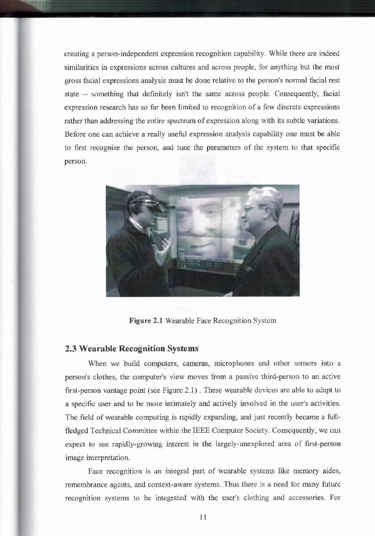
Figure 2.1 Wearable Face Recognition System

2.3 Wearable Recognition SystemsWhen we build computers, cameras, microphones and other sensors into a

person's clothes, the computer's view moves from a passive third-person to an active

first-person vantage point (see Figure 2.1) . These wearable devices are able to adapt to

a specific user and to be more intimately and actively involved in the user's activities.

The field of wearable computing is rapidly expanding, and just recently became a full­

fledged Technical Committee within the IEEE Computer Society. Consequently, we can

expect to see rapidly-growing interest in the largely-unexplored area of first-person

image interpretation.

Face recognition is an integral part of wearable systems like memory aides,

remembrance agents, and context-aware systems. Thus there is a need for many future

recognition systems to be integrated with the user's clothing and accessories. For

11

----

instance, if you build a camera into your eyeglasses, then face recognition software can

help you remember the name of the person you are looking at by whispering their name

in your ear. Such devices are beginning to be tested by the US Army for use by border

guards in Bosnia, and by researchers at the University of Rochester's Center for Future

Health for use by Alzheimer's patients.

.x,

Fusicıınoi~h ifflıd --~

Figure 2.2 Multi-modal Person Recognition System

2.4 Future of Face Recognition TechnologyFace recognition systems used today work very well under constrained

conditions, although all systems work much better with frontal mug-shot images and

constant lighting. All current face recognition algorithms fail under the vastly varying

conditions under which humans need to and are able to identify other people. Next

generation person recognition systems will need to recognize people in real-time and in

much less constrained situations.We believe that identification systems that are robust in natural environments, in

the presence of noise and illumination changes, cannot rely on a single modality, so that

fusion with other modalities is essential (see Figure 2.2). Technology used in smart

12

environments has to be unobtrusive and allow users to act freely. Wearable systems in

particular require their sensing technology to be small, low powered and easily

integrable with the user's clothing. Considering all the requirements, identification

systems that use face recognition and speaker identification seem to us to have the most

potential for wide-spread application.

Cameras and microphones today are very small, light-weight and have been

successfully integrated with wearable systems. Audio and video based recognition

systems have the critical advantage that they use the modalities humans use for

recognition. Finally, researchers are beginning to demonstrate that unobtrusive audio­

and-video based person identification systems can achieve high recognition rates

without requiring the user to be in highly controlled environments .

2.5 Geometrical FeaturesMany people have explored geometrical feature based methods for face

recognition. Kanade [5] presented an automatic feature extraction method based on

ratios of distances and reported a recognition rate of between 45-75% with a database of

20 people. Brunelli and Poggio [6] compute a set of geometrical features such as nose

width and length, mouth position, and chin shape. They report a 90% recognition rate

on a database of 47 people. However, they show that a simple template matching

scheme provides 100% recognition for the same database. Cox et al. [7] have recently

introduced a mixture-distance technique which achieves a recognition rate of95% using

a query database of 95 images from a total of 685 individuals. Each face is represented

by 30 manually extracted distances.Systems which employ precisely measured distances between features may be

most useful for finding possible matches in a large mugshot database. For other

applications, automatic identification of these points would be required, and the

resulting system would be dependent on the accuracy of the feature location algorithm.

Current algorithms for automatic location of feature points do not provide a high degree

of accuracy and require considerable computational capacity [8].

2.6 EigenfacesHigh-level recognition tasks are typically modeled with many stages of

processing as in the Marr paradigm of progressing from images to surfaces to three-

13

dimensional models to matched models [9]. However, Turk and Pentland [10] argue

that it is likely that there is also a recognition process based on low-level, two­

dimensional image processing. Their argument is based on the early development and

extreme rapidity of face recognition in humans, and on physiological experiments in

monkey cortex which claim to have isolated neurons that respond selectively to faces

[11]. However, it is not clear that these experiments exclude the sole operation of the

Marr paradigm.

Turk and Pentland [10] present a face recognition scheme in which face images

are projected onto the principal components of the original set of training images. The-

resulting eigenfaces are classified by comparison with known individuals.

Turk and Pentland present results on a database of 16 subjects with various head

orientation, scaling, and lighting. Their images appear identical otherwise with little

variation in facial expression, facial details, pose, etc. For lighting, orientation, and

scale variation their system achieves 96%, 85% and 64% correct classification

respectively. Scale is renormalized to the eigenface size based on an estimate of the

head size. The middle of the faces is accentuated, reducing any negative affect of

changing hairstyle and backgrounds.

In Pentland et al. [12,13] good results are reported on a large database (95%

recognition of 200 people from a database of 3,000). It is difficult to draw broad

conclusions as many of the images of the same people look very similar, and the

database has accurate registration and alignment [14]. In Moghaddam and Pentland

[14], very good results are reported with the FERET database - only one mistake was

made in classifying 150 frontal view images. The system used extensive preprocessing

for head location, feature detection, and normalization for the geometry of the face,

translation, lighting, contrast, rotation, and scale.

Swets and Weng [15] present a method of selecting discriminant eigenfeatures

using multi-dimensional linear discriminant analysis. They present methods for

determining the Most Expressive Features (MEF) and the Most Discriminatory Features

(MDF). We are not currently aware of the availability of results which are comparable

with those of eigenfaces (e.g. on the FERET database as in Moghaddam and Pentland

[14]).

In summary, it appears that eigenfaces is a fast, simple, and practical algorithm.

However, it may be limited because optimal performance requires a high degree of

14

------

correlation between the pixel intensities of the training and test images. This limitation

has been addressed by using extensive preprocessing to normalize the images.

2. 7 Template Matching

Template matching methods such as [6] operate by performing direct correlation

of image segments. Template matching is only effective when the query images have

the same scale, orientation, and illumination as the training images [7].

2.8 Graph Matching

Another approach to face recognition is the well known method of Graph

Matching. In [16], Lades et al. present a Dynamic Link Architecture for distortion

invariant object recognition which employs elastic graph matching to find the closest

stored graph. Objects are represented with sparse graphs whose vertices are labeled with

a multi-resolution description in terms of a local power spectrum, and whose edges are

labeled with geometrical distances. They present good results with a database of 87

people and test images composed of different expressions and faces turned 15 degrees.

The matching process is computationally expensive, taking roughly 25 seconds to

compare an image with 87 stored objects when using a parallel machine with 23

transputers. Wiskott et al. [17] use an updated version of the technique and compare 300

faces against 300 different faces of the same people taken from the FERET database.

They report a recognition rate of 97.3%. The recognition time for this system was not

gıven.

2.9 Neural Network Approaches

Much of the present literature on face recognition with neural networks presents

results with only a small number of classes (often below 20). We briefly describe a

couple of approaches.

In [18] the first 50 principal components of the images are extracted and reduced

to 5 dimensions using an autoassociative neural network. The resulting representation is

classified using a standard multi-layer perceptron. Good results are reported but the

database is quite simple: the pictures are manually aligned and there is no lighting

variation, rotation, or tilting. There are 20 people in the database.

15

A hierarchical neural network which is grown automatically and not trained with

gradient-descent was used for face recognition by Weng and Huang [19]. They report

good results for discrimination of ten distinctive subjects.

2.10 The ORL Database In [20] a HMM-based approach is used for classification of the ORL database

images. The best model resulted in a 13% error rate. Samaria also performed extensive

tests using the popular eigenfaces algorithm [10] on the ORL database and reported a

best error rate of around 10% when the number of eigenfaces was between 175 and 199.

We implemented the eigenfaces algorithm and also observed around 10% error. In [21]

Samaria extends the top-down HMM of [20] with pseudo two-dimensional HMMs. The

error rate reduces to 5% at the expense of high computational complexity - a single

classification takes four minutes on a Sun Spare II. Samaria notes that although an

increased recognition rate was achieved the segmentation obtained with the pseudo two­

dimensional HMMs appeared quite erratic. Samaria uses the same training and test set

sizes as we do (200 training images and 200 test images with no overlap between the

two sets). The 5% error rate is the best error rate previously reported for the ORL

database that we are aware o£

2.11 Related Works Henry Rowley et. al. [53] have built another neural network-based face detection

system. They first preprocess the image window and then pass it through neural

network to see whether it is a face. Their networks have three types of hidden units: 4

looking at 1 Oxl O pixel subregions, 16 looking at 5x5 pixel subregions and 6 looking at

20x5 pixel subregions. These subregions are chosen to represent facial features that are

important to face detection. Overlapping detections are merged. To improve the

performance of their system, multiple networks are applied. They are trained under

different initial condition and have different self-selected negative examples. The

outputs of these networks are arbitrated to produce the final decision.

Roberto Brunelli and Tomaso Poggio [54] develop two algorithms for face

recognition: geometric feature based matching and template matching. The geometric

feature based matching approach extracts 3 5 facial features automatically such as

eyebrow thickness and vertical position, nose vertical position and width, chin shape

16

and zygomatic breadth. These features form a 35-D vector and recognition is performed

with a Bayes classifier. In the template matching approach, each person is represented

by an image and four masks representing eyes, nose, mouth and face. Recognition is

based on the normalized cross correlation between the unclassfied image and the

database images, each of which returns a vector of matching scores (one per feature).

The person is classified as the one with the highest cumulative score. They also perform

recognition based on single feature and features are sorted by decreasing perform.ace as

eyes, nose, mouth and whole face template.

A face recognition system Visionics Facelt wins the "FERET" face recognition

test 1996 hold by the US Army Research Laboratory. It was originally developed from

the Computational Neuroscience Laboratory at The Rockefeller University. Their face

recognition is based on factorial coding which transforms the image pattern into a large

set of simpler statistically independent elements. The system finds and recognizes face

in real time. User can create their own face database and add new person to the

database. People can be gathered into different groups. A useful functionality is to

unlock the screen if the system recognizes the person. Currently it runs under Windows

95/NT with VFW or MIL video capture device driver and IRIX system 5 with an

external video camero such as SGI IndyCam.

2.12 Karhunen-Loeve Transform The optimal linear method for reducing redundancy in a dataset is the Karhunen­

Loeve (KL) transform or eigenvector expansion via Principle Components Analysis

(PCA) [22]. PCA generates a set of orthogonal axes of projections known as the

principal components, or the eigenvectors, of the input data distribution in the order of

decreasing variance. The KL transform is a well known statistical method for feature

extraction and multivariate data projection and has been used widely in pattern

recognition, signal processing, image processing, and data analysis. Points in an n­

dimensional input space are projected into an m-dimensional space, m'91. The KL

transform is used here for comparison with the SOM in the dimensionality reduction of

the local image samples. The KL transform is also used in eigenfaces, however in that

case it is used on the entire images whereas it is only used on small local image samples

in this work.

17

2.13 Convolutional Networks

The problem of face recognition from 2D images is typically very ill-posed, i.e.

there are many models which fit the training points well but do not generalize well to

unseen images. In other words, there are not enough training points in the space created

by the input images in order to allow accurate estimation of class probabilities

throughout the input space. Additionally, for MLP networks with the 2D images as

input, there is no invariance to translation or local deformation of the images [23].

Convolutional networks (CN) incorporate constraints and achieve some degree of shift

and deformation invariance using three ideas: local receptive fields, shared weights, and

spatial subsampling. The use of shared weights also reduces the number of parameters

in the system aiding generalization. Convolutional networks have been successfully

applied to character recognition [24,25,23,26,27].

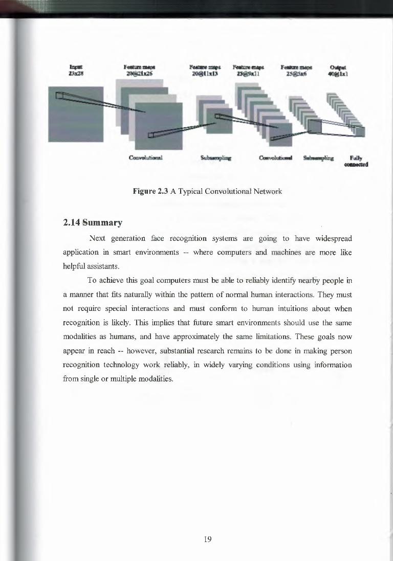
A typical convolutional network is shown in figure 2.3 [24]. The network

consists of a set of layers each of which contains one or more planes. Approximately

centered and normalized images enter at the input layer. Each unit in a plane receives

input from a small neighborhood in the planes of the previous layer. The idea of

connecting units to local receptive fields dates back to the 1960s with the perceptron

and Hubel and Wiesel's [28] discovery of locally sensitive, orientation-selective neurons

in the cat's visual system [23]. The weights forming the receptive field for a plane are

forced to be equal at all points in the plane. Each plane can be considered as a feature

map which has a fixed feature detector that is convolved with a local window which is

scanned over the planes in the previous layer. Multiple planes are usually used in each

layer so that multiple features can be detected. These layers are called convolutional

layers. Once a feature has been detected, its exact location is less important. Hence, the

convolutional layers are typically followed by another layer which does a local

averaging and subsampling operation (e.g. for a subsampling factor of 2:

Yij=(X2i,2j + X2i+ 1,2}+ 1 + X2i+ 1,2}+ 1)/4 where yij is the output of a subsampling

plane at position i, j and Xij is the output of the same plane in the previous layer). The

network is trained with the usual backpropagation gradient-descent procedure [29]. A

connection strategy can be used to reduce the number of weights in the network. For

example, with reference to figure 2.3, Le Cun et al. [24] connect the feature maps in the

second convolutional layer only to 1 or 2 of the maps in the first subsampling layer (the

connection strategy was chosen manually).

18

O!ıfe •.... .. lxl

Figure 2.3 A Typical Convolutional Network

2.14 ,Summary

Next generation face recognition systems are going to have widespread

application in smart environments -- where computers and machines are more like

helpful assistants.

To achieve this goal computers must be able to reliably identifynearby people in

a manner that fits naturally within the pattern of normal human interactions. They must

not require special interactions and must conform to human intuitions about when

recognition is likely. This implies that future smart environments should use the same

modalities as humans, and have approximately the same limitations. These goals now

appear in reach -- however, substantial research remains to be done in making person

recognition technology work reliably, in widely varying conditions using information

from singleor multiplemodalities.

19

CHAPTER THREE

AN AUTOMATIC SYSTEM FOR

DETECTION, RECOGNITION AND CODING OF FACES

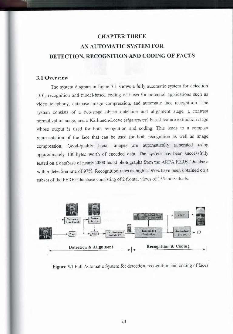
3.1 Overview The system diagram in figure 3. 1 shows a fully automatic system for detection

[30], recognition and model-based coding of faces for potential applications such as

video telephony, database image compression, and automatic face recognition. The

system consists of a two-stage object detection and alignment stage, a contrast

normalization stage, and a Karhunen-Loeve (eigenspace) based feature extraction stage

whose output is used for both recognition and coding. This leads to a compact

representation of the face that can be used for both recognition as well as ımage

compressıon. Good-quality facial images are automatically generated usıng

approximately 100-bytes worth of encoded data. The system has been successfully

tested on a database of nearly 2000 facial photographs from the ARPA FERET database

with a detection rate of 97%. Recognition rates as high as 99% have been obtained on a

subset of the FERET database consisting of 2 frontal views of 155 individuals.

Detection & Alignment Recognition & Coding

Figure 3.1 Full Automatic System for detection, recognition and coding of faces

20

3.2 Detection and Alignment

Face :viasRing ands'1 •• Comrast Xorm.

Original InputImage

Estimated Head Head-Centered Estimated Facial Warped, MaskLocation & scale Image Feature Location Facial Region

Figure 3.2 Detection and Alignment

The process of face detection and alignment consists of a two-stage object

detection and alignment stage, a contrast normalization stage, and a feature extraction

stage whose output is used for both recognition and coding. Figure 3.1 above illustrate

the operation of the detection and alignment stage on a natural test image containing a

human face.

The first step in this process is illustrated in "Estimated Head Position and

Scale" where the ML estimate of the position and scale of the face are indicated by the

cross-hairs and bounding box. Once these regions have been identified, the estimated

scale and position are used to normalize for translation and scale, yielding a standard

"head-in-the-box" format image. A second feature detection stage operates at this fixed

scale to estimate the position of 4 facial features: the left and right eyes, the tip of the

nose and the center of the mouth. Once the facial features have been detected, the face

21

--- ---------

image is warped to align the geometry and shape of the face with that of a canonical

model. Then the facial region is extracted (by applying a fixed mask) and subsequently

normalized for contrast.

3.3 Recognition and Coding

Raw 3.2 KBytes JPEG 530 Bytes

Compare

85 Bytes

"Ma yor White"

Figure 3.3 Recognition and Coding

Once the image is suitably normalized with respect to individual geometry and

contrast, it is projected onto a set of normalized eigenfaces. The figure 3.3 above shows

the first few eigenfaces obtained from a KL expansion on an ensemble of 500

normalized faces. In the system, the projection coefficients are used to index through a

database to perform identity verification and recognition using a nearest-neighbor

search.

Figure 3.4 The First 8 Normalized Eigenfaces

22

In figure 3.4, the geometrically aligned and normalized image is projected onto a

custom set of eigenfaces to obtain a feature vector, which is used for recognition

purposes as well as facial image coding.

3.4 Eigenfaces Demo

Most face recognition experiments to date have had at most a few hundred faces.

Thus how face recognition performance scales with the number of faces is almost

completely unknown. In order to have an estimate of the recognition performance on

much larger databases, we have conducted tests on a database of 7,562 images of

approximately 3,000 people.

The eigenfaces for this database were approximated using a principal

components analysis on a representative sample of 128 faces. Recognition and matching

was subsequently performed using the first 20 eigenvectors. In addition, each image

was then annotated (by hand) as to sex, race, approximate age, facial expression, and

other salient features. Almost every person has at least two images in the database;

several people have many images with varying expressions, headwear, facial hair, etc.

Figure 3.4 Standard Eigenfaces

This database can be interactively searched using an X-windows browsing tool

called Photo book. The user begins by selecting the types of faces they wish to examine;

e.g., senior Caucasian males with mustaches, or adult Hispanic females with hats. This

subset selection is accomplished using an object-oriented database to search through the

23

------

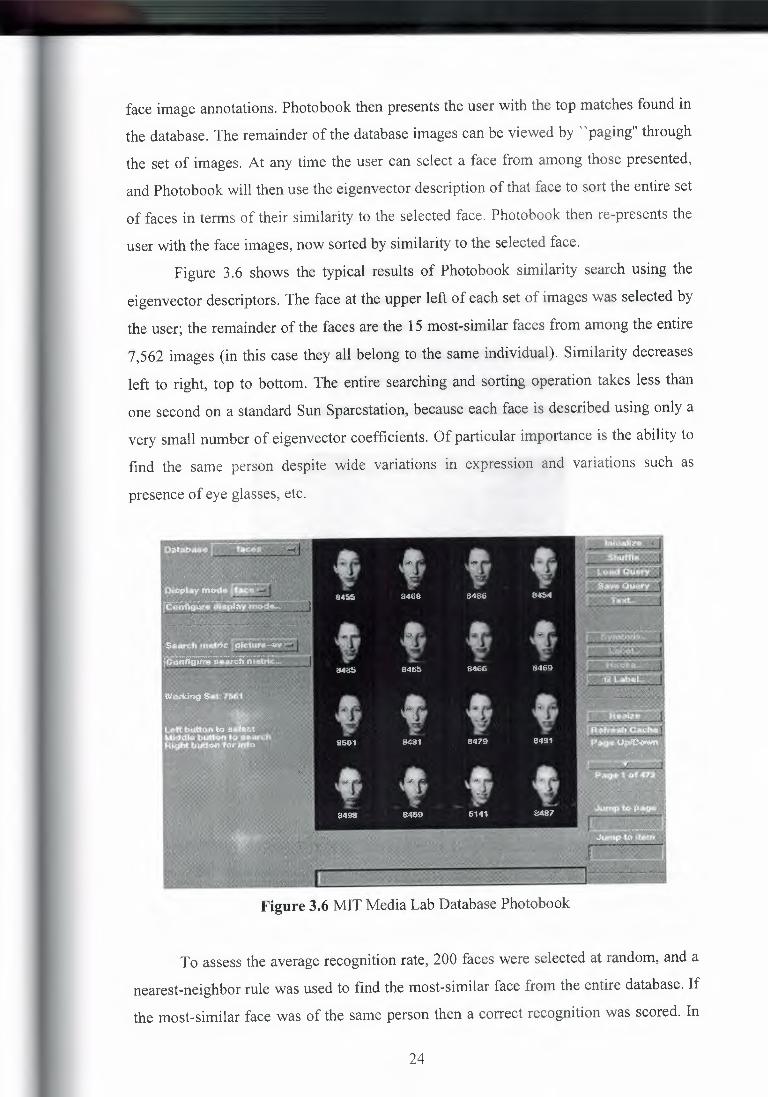
face image annotations. Photobook then presents the user with the top matches found in

the database. The remainder of the database images can be viewed by "paging" through

the set of images. At any time the user can select a face from among those presented,

and Photo book will then use the eigenvector description of that face to sort the entire set

of faces in terms of their similarity to the selected face. Photo book then re-presents the

user with the face images, now sorted by similarity to the selected face.

Figure 3.6 shows the typical results of Photobook similarity search using the

eigenvector descriptors. The face at the upper left of each set of images was selected by

the user; the remainder of the faces are the 15 most-similar faces from among the entire

7,562 images (in this case they all belong to the same individual). Similarity decreases

left to right, top to bottom. The entire searching and sorting operation takes less than

one second on a standard Sun Sparcstation, because each face is described using only a

very small number of eigenvector coefficients. Of particular importance is the ability to

find the same person despite wide variations in expression and variations such as

presence of eye glasses, etc.

Figure 3.6 MIT Media Lab Database Photobook

To assess the average recognition rate, 200 faces were selected at random, and a

nearest-neighbor rule was used to find the most-similar face from the entire database. If

the most-similar face was of the same person then a correct recognition was scored. In

24

this experiment the eigenvector-based recognition system produced a recognition

accuracy of 95%.

3.5 Modular Eigenspaces: Detection, Coding & Recognition

The eigenface technique is easily extended to the description and coding of

facial features, yielding eigeneyes, eigennoses and eigenmouths. Eye-movement studies

indicate that these particular facial features represent important landmarks for fixation,

especially in an attentive discrimination task. Therefore we should expect an

improvement in recognition performance by incorporating an additional layer of

description in terms of facial features. This can be viewed as either a modular or layered

representation of a face, where a coarse (low-resolution) description of the whole head

is augmented by additional (higher-resolution) details in terms of salient facial features.

Figure 3.7 Facial Feature Domains

With this modular technique we require an automatic method for detecting these

features. The standard detection paradigm in computer vision is that of simple

correlation or template matching. The eigenspace formulation, however, leads to a

powerful alternative to simple template matching. The reconstruction error ( or residual)

of the principal component representation (referred to as the distance-from-face-space)

is a an effective indicator of a match. The residual error is easily computed using the

projection coefficients and signal energy. This detection strategy is equivalent to

25

matching with eigentemplates and allows for a greater range of distortions in the input

signal (including lighting, rotation and scale) .

. In the eigenfeature representation the equivalent "distance-from-feature-space"

(DFFS) is effectively used for the detection of features. Given an input image, a feature

distance-map is built by computing the DFFS at each pixel. The globl minimim of this

distance map is then selected as the best feature match. This parallel search process is

illustrated in figures 3.8, 3.9.

Figure 3.8 Input Image

26

----

Figure 3.9 Feature Detections

27

-------

3.6 Detection Performance on a Large Database

Figure 3.10 Training Templates

The DFFS feature detector was used for the automatic detection and coding of

the facial feautres in our large data base of 7562 faces. A representative sample of 128

individuals was used to find a set of eigen features. Above you can see examples of

training templates used for the facial features (left-eye, right_eye, nose and mouth). The

entire database is processed by using independent detectors for each feature ( with the

DFFS computed based on projection on hte first 10 eigenvectors) The mathches are

obtained by independently selecting the global minimum in each of the four distance

maps. Typical detections are shown in figure 3 .1 1 .

28

Figure 3.11 Typical detection

Figure 3.12 Receiver Operating Characteristics: Left-Eye Detection

29

--·---·

The DFFS metric associated with each detection can be used in conjunction with

a threshold --- i.e. only the global minima with a DFFS value less than the threshold are

declared to be a possible match. Consequently we can characterize the detection vs.

false-alarm tradeoff by varying this threshold and generating a receiver operating

characteristics (ROC) curve. Figure above shows the ROC curve for the left eye (the left

eye is the feature which was most accurately registered in the image, thus providing the

most reliable ROC curve). A correct detection was defined as a below-threshold global

minimum within 5 pixels of the mean left eye position. Similarly, a false alarm was

defined as a below-threshold detection located outside the 5-pixel radius. Global

minima above the threshold were undeclared. The peak performance of this detector

corresponds to a 94% detection rate at a false alarm rate of 6%. Conversely, at a zero

false-alarm rate, 52% of the eyes were correctly detected. To calibrate the performance

of the DFFS detector, we have also shown the ROC curve corresponding to a standard

sum-of-square-differences (SSD) template matching technique. The templates used

were the mean features in each case.

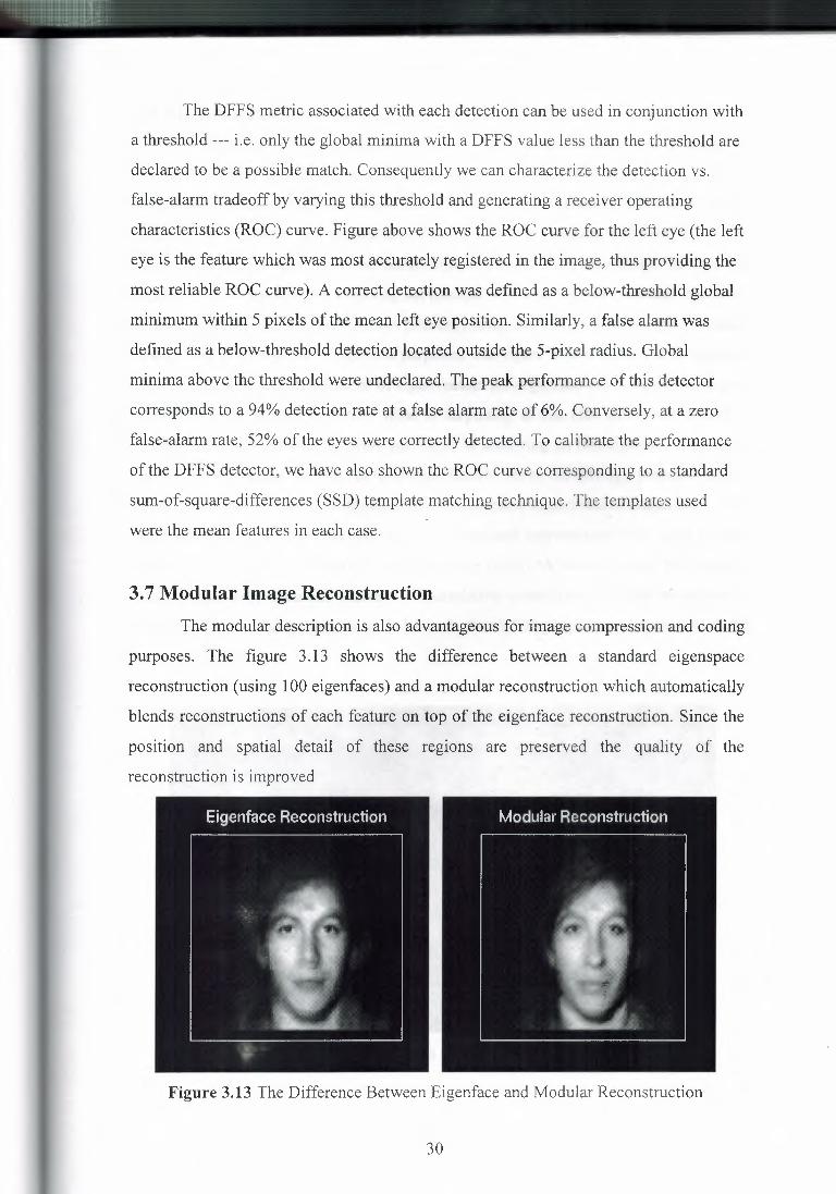
3.7 Modular Image Reconstruction The modular description is also advantageous for image compression and coding

purposes. The figure 3.13 shows the difference between a standard eigenspace

reconstruction (using 100 eigenfaces) and a modular reconstruction which automatically

blends reconstructions of each feature on top of the eigenface reconstruction. Since the

position and spatial detail of these regions are preserved the quality of the

reconstruction is improved

Figure 3.13 The Difference Between Eigenface and Modular Reconstruction

30

3.8 Modular Recognition

With the ability to reliably detect facial features across a wide range of faces, we

can automatically generate a modular representation of a face. The utility of this layered

representation (eigenface plus eigenfeatures) was tested on a small subset of our face

database. We selected a representative sample of 45 individuals with two views per

person, corresponding to different facial expressions (neutral vs. smiling). These set of

images was partitioned into a training set (neutral) and a testing set (smiling). Since the

difference in the facial expressions is primarily articulated in the mouth, this particular

feature was discarded for recognition purposes. The figure below shows the recognition

rates as a function of the number of eigenvectors for eigenface-only, eigenfeature-only

and the combined representation. What is surprising is that (for this small dataset at

least) the eigenfeatures alone were sufficient in achieving an (asymptotic) recognition

rate of 95% (equal to that of the eigenfaces). More surprising, perhaps, is the

observation that in the lower dimensions of eigenspace, eigenfeatures outperformed the

eigenface recognition. Finally, by using the combined representation, we gain a slight

improvement in the asymptotic recognition rate (98%). A similar effect has recently

been reported by Brunelli where the cumulative normalized correlation scores of

templates for the face, eyes, nose and mouth showed improved performance over the

face-only recognition.

Figure 3.14 Recognition Rates Of Multi-layered Representation

31

---

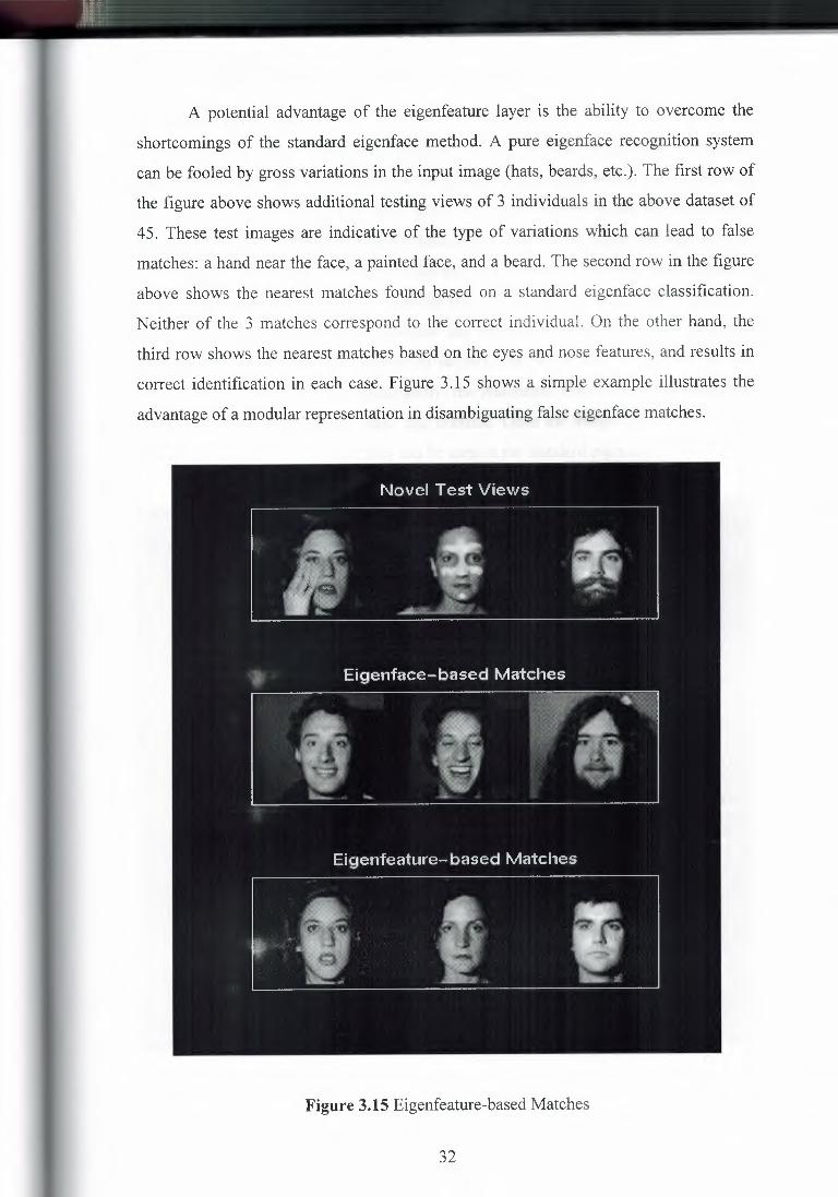
A potential advantage of the eigenfeature layer is the ability to overcome the

shortcomings of the standard eigenface method. A pure eigenface recognition system

can be fooled by gross variations in the input image (hats, beards, etc.). The first row of

the figure above shows additional testing views of 3 individuals in the above dataset of

45. These test images are indicative of the type of variations which can lead to false

matches: a hand near the face, a painted face, and a beard. The second row in the figure

above shows the nearest matches found based on a standard eigenface classification.

Neither of the 3 matches correspond to the correct individual. On the other hand, the

third row shows the nearest matches based on the eyes and nose features, and results in

correct identification in each case. Figure 3 .15 shows a simple example illustrates the

advantage of a modular representation in disambiguating false eigenface matches.

Figure 3.15 Eigenfeature-based Matches

32

3.9 Summary It is a developmeant of an automatic system for recognition and interactive

search in the FERET face database. A recognition accuracy of 99.35% was obtained

using two frontal views of 155 individuals. The figure below shows the result of a

typical similarity search on the FERET database. The face at the upper left was selected

by the user; the remainder of the faces are the most-similar faces from the 575 frontal

views in the FERET database. Note that the first four images (in the top row) are all of

the same individual (with/without glasses and different expressions). Also note this

database represents a realistic application scenario where position, scale, lighting and

background are not uniform. Consequently, the Automatic Face Processing System is

used to correct for translation, scale, and contrast. Once the images are geometrically

and photometrically normalized, they can be used in the standard eigenface technique.

Figure 3.16 Automatic Face Processing System

33

- -------

CHAPTER FOUR

FACE RECOGNITION BY

DYNAMIC LINK MATCIIlNG

4.1 Overview

The intracortical wiring pattern is a fascinating scientific subject, as it seems to

hold the key to the function of the brain, or the part of it that we are accustomed to take

most seriously. That wiring pattern is unnervingly close to being all-to-all. It has been

speculated that signals from any cell in cortex can reach any other by crossing just three

synapses. Although this seems to make sense for a system in which any two data items

may have to contact each other, near-to-complete wiring seems to leave little room for

all the specific structure that according to our present view of the brain resides in its

connections. The experimental techniques of anatomy and neurophysiology are much

too limited to give us more than gross principles of a cortical wiring pattern. These

principles are to a very large extent summarized by speaking about receptive field

structures, columnar organization, regular local interactions of the general type of

difference-of-Gaussians and topographical connection patterns between areas. Beyond

that we are in a dark continent, which may, for all we know, be dominated by

randomness. More likely, however, it is structured by intricate learned patterns that are

too variable from individual to individual and from place to place to ever become a

possible subject of experimental enquiry.We are presenting here a model for invariant object recognition, together with

tests on human face recognition from a large gallery. The model may be relevant to the

discussion at hand since it makes minimal assumptions about genetically generated

connection patterns --- certainly none that go beyond the principles enumerated --- and

relies largely on rapid reversible synaptic seff-organizarion during the recognitionprocess to create the much more specific connections required for a concrete recognition

act. The model relies on Dynamic Link Matching (DLM) the qualitative principle. The

model described here goes beyond previously published versions in being more

complete in its dynamic formulation, including mechanisms for autonomous activity

blob dynamics, attention dynamics, and dynamic interaction between the stored models

to implementthe actual decisionprocess during recognition.

34

A few words are in order to relate the jargon used in the description of the model

to the biological background. The term image refers to a cortical image domain which

corresponds to the primary visual cortex V1 and possibly also to other areas up to

perhaps V4. The image or image domain has the form of a graph. The nodes of the

graph correspond to hypercolumns, that is, to collections of those feature specific

neurons that are activated from one retinal point. In our system we formalize the activity

of the sets of feature cells within hypercolumns as jets. As features we use Gabor-based

wavelets. The links of the image graph correspond to lateral connections between

nodes. An image on the retina selects a subset of the feature cells in the image domain.

The selected neurons are then stochastically activated (these fluctuations not being

driven by the visual signal). It is important that this stochastic activity takes a form that

is characterized by temporal short-range correlations. These correlations express the

neighborhood relations of visual features in the image and are produced by the lateral

connections within the image domain. In our specific system the stochastic signal in the

image domain (and also in the model domain) has the form of a local running blob of

activity that is confined to an attention window. Apart from the local correlations the

details of the activity process are not important, however.

The models (see right side of Figure 4.1) collectively form the model domain.

We imagine this to be identified with some part of inferotemporal cortex. The nodes of

the models again have the form ofjets and are collections of neurons carrying feature

labels. They are laterally connected much like nodes in the image domain. In our system

the different models are totally disjoint. In the biological case models are likely to have

partial overlap, in terms of single nodes or even partial networks. The stochastic activity

process in the models is similar to that in the image domain, except for the interactions

between models, which have the form of local co-operation (correlating activity

between structurally corresponding points) and global competition between entire

models.The image domain and the model domain are bi-directionally connected by

dynamic links. These correspond to connections between primary and infero-temporal

cortex. These connections are assumed to be plastic on a fast time scale (changing

radically during a single recognition event), this plasticity being reversible. The strength

of a connection between any two nodes in the image and a model is controlled by the jet

similarity between them, which roughly corresponds to the number of features that are

common to the two nodes.

35

4.2 Architecture and DynamicsFigure 4.1 shows the general architecture of the system.Faces are represented as

rectangular graphs by layers of neurons. Each neuron represents a node and has a jet

attached. A jet is a local description of the grey-value distribution based on the Gabor

transform (39,50]Topographical relationships between nodes are encoded by excitatory and inhibitory

lateral connections. The model graphs are scaled horizontally and vertically and aligned

manually, such that certain nodes of the graphs are placed on the eyes and the mouth

(cf the Data Base section). Model layers (lOxlO neurons) are smaller than the image

layer (16x17 neurons). Since the face in the image may be arbitrarily translated, the

connectivity between model and image domain has to be all-to-all initially. The

connectivity matrices are initialized using the similarities between the jets of the

connected neurons. DLM serves as a process to restructure the connectivity matrices

and to find the correct mapping between the models and the image (see Figure 4.2). The

models cooperate with the image depending on their similarity. A simple winner-take­

all mechanism sequentially rules out the least active and least similar models, and the

best-fitting one eventually survives.(

(

~...I •I~

n..•

ımage

models

Figure 4.1 Architecture of the DLM Face Recognition System

36

-- .. ----··-- --- ~-

Several models are stored as neural layers of local features on a 1 Oxl O grid, as

indicated by the black dots. A new image is represented by a 16xl 7 layer of nodes.

Initially, the image is connected all-to-all with the models. The task of DLM is to find

the correct mapping between the image and the models, providing translational

invariance and robustness against distortion. Once the correct mapping is found, a

simple winner-take-all mechanism can detect the model that is most active and most

similarto the image.

Figure 4.2 Initial and Final Connectivity for OLM

Image and model are represented by layers of l 6x17 and I Ox I O nodes

respectively. Each node is labeled with a local feature indicated by small texture

patterns. Initially, the image layer and the model layer are connected all-to-all with

synaptic weights depending on the feature similaritiesof the connected nodes, indicated

by arrows of different line widths. The task of DLM is to select the correct links and

establish a regular one-to-one mapping. We see here the initial connectivity at t = O and

37

the final one at t = 10000. Since the connectivity between a model and the image is a

four-dimensional matrix, it is difficult to visualize it in an intuitive way. If the rows of

each layer are concatenated to a vector, top row first, the connectivity matrix becomes

two-dimensional. The model index increases from left to right, the image index from

top to bottom. High similarityvalues are indicated by black squares. A second way to

illustrate the connectivity is the net display shown at the right. The image layer serves

as a canvas on which the model layer is drawn as a net. Each node corresponds to a

model neuron, neighboring neurons are connected by an edge. The location of the nodes

indicate the center of gravity of the projective field of the model neurons considering

synaptic weights as physicalmass. In order to favor strong links, the masses are taken to

the power of three. (see Figure 4.5 for connectivitydevelopment in time)

The dynamics on each layer is such that it produces a running blob of activity

which moves continuously over the whole layer. An activity blob can easily be

generated from noise by local excitation and global inhibition . It is caused to move by

delayed self-inhibition, which also serves as a memory for the locations where the blob

has recently been. Since the models are aligned with each other, it is reasonable to

enforce alignment between their running blobs by excitatory connections between

neurons representing the same facial location. The blobs on the image and the model

layers cooperate through the connection matrices; they tend to align and induce

correlations between corresponding neurons. Then, fast synaptic plasticity and a

normalization rule coherently modify the synaptic weights., and the correct

connectivities between models and image layer can develop. Since the models get

different input from the image, they differ in their total activity. The model with

strongest connections from the image is the most active one. The models compete on

the basis of their total activity. After a while the winner-take-all mechanism suppresses

the least competitive models, and eventually only the best model survives. Since the

image layer may be significantlylarger than the model layers, we introduce an attention

window in form of a large blob. It interacts with the running blob, restricts its region of

motion, and can be shifted by it to the actual face position.

The equations of the system are given in Table 4.1; the respective symbols are

listed in Table 4.2. In the following sections, we will explain the system step by step:

blob formation, blob mobilization, interaction between two layers, link dynamics,

attention dynamics, and recognition dynamics; in order to make the description clearer,

parts of the equations in Table 4.1 corresponding to these functions will be repeated.

38

-·~·----

Table 4.1 Formulas of the DLM Face Recognition System

Layer dyaamics:hf{to) =

hf (t) =

,ıf (to}~(t}

o. LP ~ ( lhP' }.) f:ı. '""" (h· P ) JI-ııi + .t- max Ut-ı1u\ • i' . - ¥h .t- u is' .. - tı:.ıu~

i' rı i'

+"Aıı mr (Wfl tr{kj)) + 1tıı,~ (a(ıır,) - ,8'1t°,) - tfe0(re - rP)

- o

a(h)h:S;OO<h<p h2.p

Attention dynarııiöli:af (to.) = nJırN(..1f)

b.''('t) = l (-a.P + ""'~ ,,,-'al!) - ~ ~ ırlol' }- + ıt-"--a(Ji'))i Q . J .L-ıı__ . .1~-·-" \,'. f'C- .L...ı- .. \ ··i1. ..•••.• . ,··-.f ·_ .·

" i'

Link dynamics:W~4(te.) :;:;: &!J = ma.'f. (S"'.(3l'. :IJ), as)

Y.V,'7(t) = .:\w (u{~ltr(h,)-S ( ,,~fWJ;/~)-ı)) Wfl

Recognition dynamics:rR(to.) = l

i-P(t) = >.r,.P (PP - n},ı{,.,1JV''})Ji'P(t) = Eo-cnn

(1)

(7)

39

- -- ----- -·---- --

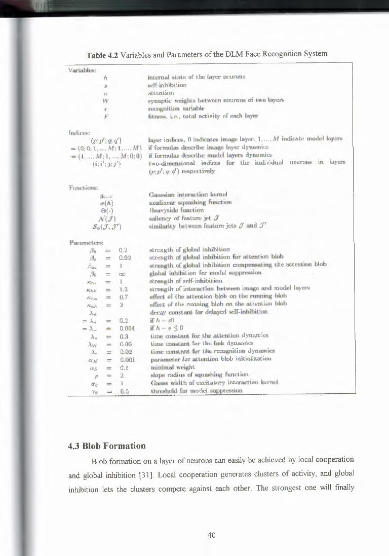
Table 4.2 Variables and Parameters of the OLM Face Recognition System

!IawrF

Jndkes;(p; p1; q; q'}

·- (O• o, 1 M·· 1 "*)- . ~ ~ . ,. ••..••.•• ?'. ~ '1 .•••..••"!" l'Vl .

= [I, ... ,M; I, .•., M;O;O}(fr•'; j;j'}

Parıımdcn:~I;; = 0...:2~.. = Q.02

fJ.,,t., - l,'J(; = 00

Keh;; - lt4Wı - l.;2,.h.. - 0.7nu = 3Jı:,:

=.\+ = o..2l!e A.. l!e 0.004

A,. - oaAw - 11.05

)ıf' - 0.02O{,'tl ; 0.001as = 0.1

p = 2n'ı - lf'& ~ 0.5

4.3 Blob Formation

internal. .ııt.at.e of the !:ayer mrumn'llsrJf~inhihitionat:tartiansynaptic weight& between nıruromı of two lıtyen.~ition variable:fitnesı., i.e.. , tohıl act.ivity of eaclı layer

laJl!f' indk\181 O indicatoo im~ layt:t\ 11 ••• t M irıdicatfımodel ~,en.ıf foclfflllM. d.eecrihe im.aı-e ·h\,tx· dyıw.miaif formulas dıescrlbe model laymı dynamicıı:lwo-diıtlCllNorud lııd.ices for the io.dividwıl nt."W'OW. in li\,J't.ff

(~ 1l;q; ,/} respı:divdy

Gaussian interaction kı~ıılnonlimıar Stıua'fthing fımotion.Htıav)'Kide fwı.ctirmeaailfltle}' qt mature jı:-t :ı~riiı:r bı:tweeıı feature jets :ı ım.d. :!'

strength: of gJobal in)n'bitionst;reu.gtlıof glt)bru inhibition for attention blobst.mngth of global inhibition mmpın:ısııting the atttınlion. blobglobal :iıtıhibition {or- model ı.,u~i,mst;mngth of ıııelf-inhlbit.ionat.mngth of interactfon between im~e and model t.ıverse:ft'eçt. of the attention blob oo t.tre running bloboffootrıf the running blob an the attımtioo blohd'.tf'.ay con~ti.m for delayed d~inlübitionif h =· sOil'l•-t1SOlıiıue amstruıt, fer the attıen.t.iou dyuamicsLiıne con.etmıt fur tlın lmk dynamiaıLi.me mmıtant for tlıe l'tlt:Q,gnİLimı dyrnınıiı:sJmranıeter for aitv.nüım blob initialiutionminimal weight$lope radius or ııquruihiııg fnnı:tiona~ ~,idth ~r ~:ırci~tıocy inwro.ct:iını ken~~\d fttr 11l.Odti ~t:m',ltın

Blob formation on a layer of neurons can easilybe achieved by local cooperation

and global inhibition [31]. Local cooperation generates clusters of activity, and global

inhibition lets the clusters compete against each other. The strongest one will finally

40

-·-·-- ..- -- ----~-~-

suppress all others and grow to an equilibrium size determined by the strengths of

cooperation and inhibition.The corresponding equations are (cf Equations 1, 3, and 4):

fu(t) (8)

u(h)

exp ( - {i ;(1~32) '(1

{

O : h<O.,/fJp ; O<h<p

. 1 : h'?;,p

(9

(Hl

The internal state of the neurons is denoted by hi , where i is a two-dimensional

Cartesian coordinate for the location of the neuron. The neurons are arranged on a

regular square lattice with spacing 1, i.e., i = (0,0), (0,1), (0,2), ... , (1,0), (1,1) , ...

The neural activity (which can be interpreted as a mean firing rate) is determined by the

squashing function oth} of the neuron's internal state h. The neurons are connected

excitatorily through the Gaussian interaction kernel g. The strength of global inhibition

is controlled by /Jh. It is obvious that a blob can only arise if Ph < go = 1 (imagine only

one neuron is active), and that the blob is larger for smaller Ph- Infinite growth of his

prevented by the decay term -h, because it is linear, while the blob formation terms

saturate due to the squashing function oth). The special shape of ath) is motivated by

three factors. Firstly, evanishes for negative values to suppress oscillations in the

simulations by preventing undershooting. Secondly, the high slope for small arguments

stabilizes small blobs and makes blob formation from low noise easier, because for

small values of &the interaction terms dominate over the decay term. Thirdly, the finite

slope region between low and high argument values allows the system to distinguish

between the inner and outer parts of the blobs by making neurons in the center of a blob

more active than at its periphery. Additional multiplicative parameters of the decay or

cooperation terms would only change time and activity scale, respectively, and do not

generate qualitatively new behavior. In this sense the parameter set is complete and

minimal.

41

-~·-------=---

4.4 Blob MobilizationGenerating a running blob can be achieved by delayed self-inhibition, which

drives the blob away from its current location; the blob generates new self-inhibitionat

the new location. This mechanism produces a continuously moving blob (see Figure

4.3). The driving force and the recollection time as to where the blob has been can be

independently controlled by their respective time constants. The corresponding

equations are (cf Equations 1 and 2):

h,(t)

a.O)

-h; + }._: (fı-f1tr(hv)) - Ph E a:(ht1) - K-h,Bi~,, ~

A:t:(~ - ~).

1)1)

(12)

The self-inhibitionsis realized by a leaky integrator with decay constant U. The

decay constant has two different values depending on whether h - s is positive or

negative. This accounts for the two different functions of the self-inhibition.The first

function is to drive the blob forward. In this case h > s, and a high decay constant U is

appropriate. The second function is to indicate where the blob has recently been, i.e., to

serve as a memory and to repel the blob from regions recently visited. In this case h < s

and a low decay constant A- is appropriate. For small layers, A- should be larger than for

large ones, because the blob visits each location more frequently. The speed of the blob

is controlled by A+ and the coupling parameter K h; They may also change the shape of

the blob. Small values such as those used in our simulations allow the blob to keep its

equilibrium shape and drive it slowly; large values produce a fast-moving blob distorted

to a kidney-shape.

42

___ ..•.,., eoı:wnuowıly moviq hlob

- - - - - .•• jllmps of dre blob

•• •=~.I I ı.sc:ı. ..•...J:~.·~· ·~· ~· " ' • ••••.cı ıııı...ıı...;.-ı.ı........ıı~l!!J.

iııııı,..,-,..ı....ı~-L.eI ,H+.,::1-f....W-U

I I :ı.111:.­k,_t : r • , er.:,_,;: Jr,

• :,u,.t:,C]C:= ·, .. , t: - I""::: In ...l- ...ı

, c ı -· a

U:U l••t:t:f tl•. "'..J·

•ı•ı·,· ~ I~ W -~····· ;ı; !I a.•. ,

•••, u3ıd Iii a•

.. ı.g •. ı: , •.••

figure 4.3 A Sequence ofLayer States as Simulated with Equations 11 and 12

The activity blob hshown in the middle row has a size of approximately six

active nodes and moves continuously over the whole layer. Its course is shown in the

upper diagram. The delayed self-inhibition s, shown in the bottom row, follows the

running blob and drives it forward. One can see the self-inhibitorytail that repels the

blob from regions just visited. Sometimes the blob runs into a trap (cf column three)

and has no way to escape from the self-inhibition. It then disappears and reappears

again somewhere else on the layer. (The temporal increment between two successive

frames is 20 time units.)

4.5 Layer Interaction and SynchronizationIn the same way as the running blob is repelled by its self-inhibitorytail, it can

also be attracted by excitatory input from another layer, as conveyed by a connection

matrix. Imagine two layers of the same size mutually connected by the identity matrix,

i.e., each neuron in one layer is connected only with the one corresponding neuron in

the other layer having the same index value. The input then is a copy of the blob of the

other layer. This favors alignment between the blobs, because then they can cooperate

and stabilize each other. This synchronizationprinciple holds also in the presence of the

noisy connection matrices generated by real image data (see Figure 4.4). The

corresponding equation is (cf. Equation 1):

43

- -·--·~--- -·---- -·- ..

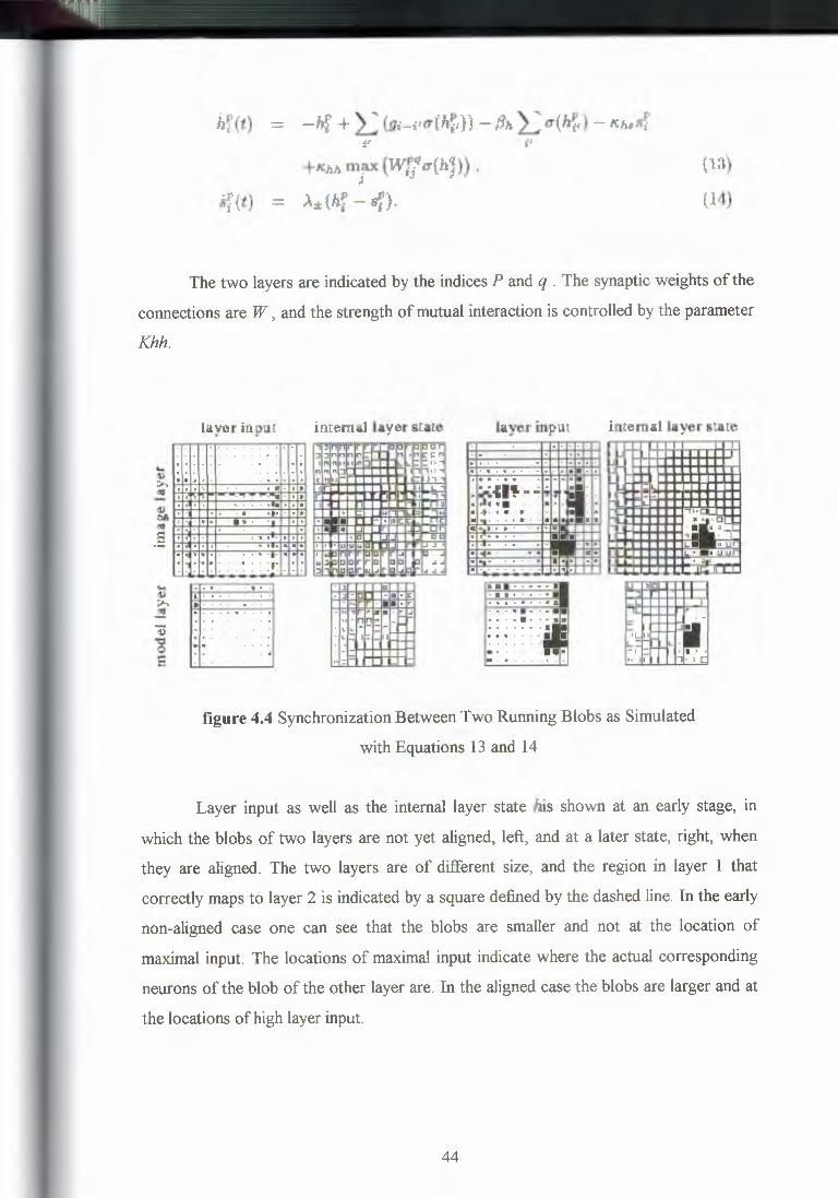
-Jıf + l.: (11,-i10:(hf,H - /J;, l:o-(bf;} - ıı:h#afi! i'

+Rlıh maJ<·(lV'.· "ı.r(h1)}·........ . cJ j., ıj

As (hf - .sf).

(1:l)

(14)

The two layers are indicated by the indices P and q . The synaptic weights of the

connections are W, and the strength of mutual interaction is controlled by the parameter

Khh.

layer input Internal l.ıyer ı;ı:at0

, ..,~,: : : : . : :: ı.~ı~ f-1~1'.:'.l-ttf_··· '.•. t:ı ,ı;n ıı...

' . ,•ı;:,-

internal fayer state

tt::::::=-m~:: ~ ~: :::::::~11uılıııııı ı ıIlayer ınp-ııt

ııı:g_fll

figure 4.4 Synchronization Between Two Running Blobs as Simulated

with Equations 13 and 14

Layer input as well as the internal layer state his shown at an early stage, in

which the blobs of two layers are not yet aligned, left, and at a later state, right, when

they are aligned. The two layers are of different size, and the region in layer I that

correctly maps to layer 2 is indicated by a square defined by the dashed line. In the early

non-aligned case one can see that the blobs are smaller and not at the location of

maximal input. The locations of maximal input indicate where the actual corresponding

neurons of the blob of the other layer are. In the aligned case the blobs are larger and at

the locations of high layer input.

44

---

4.6 Link Dynamics One principle of DLM is that the links between two layers can be cleaned up and

structured on the basis of correlations between pairs of neurons (see Figure 4.5 ). The

correlations result from the layer synchronizationdescribed in the previous section. The

link dynamics typically consists of a growing term and a normalization term. The

former lets the weights grow according to the correlation between the connected

neurons. The latter prevents the links from growing infinitely and induces competition

such that only one link per neuron survives which suppresses all others. The

corresponding equations are (cf Equations 6):

r.İıH( ·)VI'.·."' ti,.;ı

,...pq ( "" t ,rP iJ"l· )oıJ = mu S,ı,,v, ,vf),as.,

Aw ( oilıf)ıT(lıJ) - 0 {ıı,-xtwt1 ISU,) - l)) WU, (15)

Links are initialized by the similarity Srı, between the jets J of connected nodes

[49].The parameter as guarantees a minimalpositive synaptic weight, permitting each

link to suppress others, even if the similarity between the connected neurons is small.

This can be useful to obtain a continuous mapping if a link has a neighborhood of

strong links inducing high correlations between the pre- and postsynaptic neurons of the

weak link. The synaptic weights grow exponentially, controlled by the correlation

between connected neurons defined as the product of their activities ath]',)a(h/) . The

learning rate is additionally controlled by Aw . Due to the Heavyside-function 0,

normalization takes place only if links grow beyond their initial value. Then, the link

dynamics is dominated by the normalization term, with a common negative contribution

for all links converging to the same neuron. Notice that the growth term, based on the

correlation, is different for different links. Thus the link with the highest average

correlation will eventually suppress all others converging to the same neuron. Since the

similarities Srı, cannot be larger than 1, the synaptic weights W are restricted to the

interval [O, ... , 1] .

45

- - ·-

l= o 200 500 1000 1000 5 000 10000

Figure 4.5 Connectivity and Correlations Developing in Time

It can be seen how the correlations develop faster and are cleaner than the

connectivity.Both are iteratively refined on the basis of the other.

4. 7 Attention Dynamics

The alignment between the running blobs depends very much on the constraints,

ı.e., on the size and format of the layer on which they are running. This causes a

problem, since the image and the models have different sizes. We have therefore

introduced an attention blob which restricts the movement of the running blob on the

image layer to a region of about the same size as that of the model layers. Each of the

model layers also has the same attention blob to keep the conditions for their running

blobs similar to that in the image layer. This is important for the alignment. The

attention blob restricts the region for the running blob, but it can be shifted by the latter

into a region where input is especially large and favors activity. The attention blob

therefore automatically aligns with the actual face position (see Figures 4.6, 4.7 ). The

attention blob layer is initialized with a primitive segmentation cue, in this case the

norm of the respective jets [49], · since the norm indicates the presence of textures of

high contrast. The corresponding equations are (cf Equations 1 and 5):

46

- -----

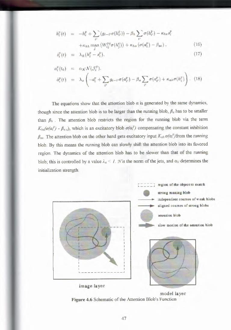
hf{t) = -hf +}.:{u,_,,.,.(h~JJ-Pı.Lo-(hf,)- .1¢A,sffi ,,

+. ıı . nıa.x (ruf_'İalh<J.}·}· +··. Jt.. (a'nf) - R. ·). hh J n,3 .. \. ;. . ..a .·· \."""I ~ııc ,

l;t:(ıı: - .(),

{16)

if(. ı)t .. (l?'

a:(to) = o.Jı.·Nt.Jf),

~{t) = A.ı (·.-ar +Eı1,-,nT(t?) .... fJıı I:a<<,) + Koh6(~))·· > (18·ı ..,t ı .

The equations show that the attention blob a is generated by the same dynamics,

though since the attention blob is to be larger than the running blob, Pa has to be smaller

than Ph . The attention blob restricts the region for the running blob via the term

Kha(a(at} - Pac), which is an excitatory blob a(at) compensating the constant inhibition

Pac- The attention blob on the other hand gets excitatory input Kah a(al)from the running

blob. By this means the running blob can slowly shift the attention blob into its favored

region. The dynamics of the attention blob has to be slower than that of the running

blob; this is controlled by a value Aa < 1 . .Wis the norm of the jets, and aN determines the

initializationstrength.

r-----,L----J reıiOll of Ilı• oltjecı ıo mımtı

ıtronı mnniııı blobio.clepıuıdeııt camın ofwnt: blohsaligned.coıuıea of strong blobii

..•..•.•. .-"1IlıIIIlIIIIII

aueo.ıioc blob

ıılo~· motion.of the aıtenrion blob

image fayer

ı;.., ---- --- - .__ .,.J

model layerFigure 4.6 Schematic of the Attention Blob's Function

47

----~

The attention blob restricts the region in which the running blob can move. The

attention blob, on the other hand, receives input from the running blob. That input will

be strong in regions where the blobs in both layers cooperate and weak where they do

not (see Figure 4.4). Due to this interaction the attention blob slowly moves to the

correct region indicated by the square made of dashed lines. The attention blob in the

model layer is required to keep the conditions for the running blobs symmetrical.

ntteoıtioııblob

image layer:runniagblob

t = 25

t= 500

t: 1000

mııııiııı blob :auentioıı blob

111:odol layer

Figure 4.7 Function of the Attention Blob, Using an Extreme Example of an Initial

Attention Blob Manually Misplaced for Demonstration

At t = 150 the two running blobs ran synchronously for a while, and the

attention blob has a long tail. The blobs then lost alignment again. From t = 500 on, the

48

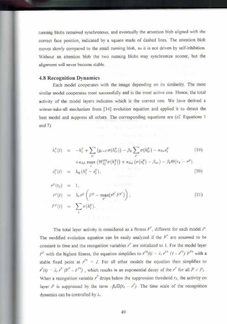
running blobs remained synchronous, and eventually the attention blob aligned with the

correct face position, indicated by a square made of dashed lines. The attention blob

moves slowly compared to the small running blob, as it is not driven by self-inhibition.

Without an attention blob the two running blobs may synchronize sooner, but the

alignment will never become stable.

4.8 Recognition Dynamics Each model cooperates with the image depending on its similarity. The most

similarmodel cooperates most successfully and is the most active one. Hence, the total

activity of the model layers indicates which is the correct one. We have derived a

winner-take-all mechanism from [34] evolution equation and applied it to detect the

best model and suppress all others. The corresponding equations are (cf Equations 1

and 7):

hf(t) (19)

- . . . .. (utP'I (1 9")· - · (. ·(, p)· ıQ 1· ıQ öc·· . J!''>+ıtü mrx . ll'tj tr ''J,. + K.ıia tr a, - !-'<JC - pl}'Q f'(J - 1 Jt

if(t) = .,\;t:(lıf - .sf). (20

rfl(to) = 1,

fP(f} = ~,,.ıı (Fl' - -,.=-t,:P' FP')) ~c, 7\ • ..

F'(t) = L6(hf).t

{21)

The total layer activity is considered as a fitnessF, different for each model P.

The modified evolution equation can be easily analyzed if the F are assumed to be

constant in time and the recognition variables ? are initializedto 1. For the model layer

pb with the·highest fitness, the equation simplifiesto l'b (t) = Ar .,Pb (1 - .,Pb) r" with a

stable fixed point at .,Pb = 1. For all other models the equation then simplifies to

I' (t) = Ar? (F - Fb) , which results in an exponential decay of the? for all Pt- Pb .

When a recognition variable ? drops below the suppression threshold re, the activity on

layer P İs suppressed by the term ~PeG(re - ?). The time scale of the recognition

dynamicscan be controlled by Ar .

49

4.9 Bidirectional Connections The connectivity between two layers is bidirectional and not unidirectional as in

the previous system [38]. This is necessary for two reasons: Firstly, by this means the

running blobs of the two connected layers can more easily align. With unidirectional

connections one blob would systematicallyrun behind the other. Secondly, connections

in both directions are necessary for a recognition system. The connections from model

to image layer are necessary to allow the models to move the attention blob in the image

into a region that fits the models well. The connections from the image to the model

layers are necessary to provide a discrimination cue as to which model best fits the

image. Otherwise, each model would exhibit the same level of activity.

4.10 Blob Alignment in the Model Domain Since faces have a common general structure, it is advantageous to align the

blobs in the model domain to insure that they are always at the same position in the

faces, either all at the left eye or all at the chin etc. This is achieved by connections

between the layers and leads to the term +"fi maxu (gi - ia(f{'iJ) instead of

+'2:i(g; - la(f{iJ) in Equation 1. If the model blobs were to run independently, the image

layer would get input from all face parts at the same time, and the blob there would

have a hard time to align with a model blob, and it would be very uncertain whether it

would be the correct one. The cooperation between the models and the image would

depend more on accidental alignment than on the similaritybetween the models and the

image, and it would then be very likely that the wrong model was picked up as the

recognition result. One alternative is to let the models inhibit each other such that only

one model can have a blob at a time. The models then would share time to match onto

the image, and the best fitting one would get most of the time. This would probably be

the appropriate setup if the models were very different and without a common structure,

as it is for general objects. The disadvantage is that the system needs much more time to

decide which model to accept, because the relative layer activities in the beginning

depend much more on chance than in the other setup.

4.11 Maximum versus Sum Neurons

The model neurons used here use the maximum over all input signals instead of

the sum. The reason is that the sum would mix up many different signals, while only

one can be the correct one, i.e., the total input would be the result of one correct signal

50

--- ------~---

and many misleadingones. Hence the signal-to-noise ratio would be very low. We have

observed an example where even a model identical to the image was not picked up as

the correct one, because the sum over all the accidental input signals favored a

completely different-looking person. For that reason we introduced the maximum input

function, which is reasonable since the correct signal is likely to be the strongest one.

The maximumrule has the additional advantage that the dynamic range of the input into

a single cell does not vary much when the connectivity develops, whereas the signal

sum would decrease significantlyduring synaptic re-organization and let the blobs loose

their alignment.

4.12 Experiments

4.12.1 Data Base As a face data base we used galleries of 111 different persons. Of most persons

there is one neutral frontal view, one frontal view of different facial expression, and two

views rotated in depth by 15 and 30 degrees respectively. The neutral frontal views

serve as a model gallery, and the other three are used as test images for recognition. The

models, i.e., the neutral frontal views, are represented by layers of size lOxlO (see

Figure 4.1). Though the grids are rectangular and regular, i.e., the spacing between the

nodes is constant for each dimension, the graphs are scaled horizontally in the x- and

vertically in the y-direction and are aligned manually: The left eye is always represented

by the node in the fourth column from the left and the third row from the top, the mouth

lies on the fourth row from the bottom, etc. The x-spacing ranges from 6.6 to 9.3 pixels

with a mean value of 8.2 and a standard deviation of0.5. They-spacing ranges from 5.5

to 8.8 pixels with a mean value of 7.3 and a standard deviation of 0.6. An input image

of a face to be recognized is represented by a 16xl7 layer with an x-spacing of 8 pixels

and a y-spacing of 7 pixels. The image graphs are not aligned, since that would already

require recognition. The variations of up to a factor of 1.5 in the x- and y-spacings must

be compensated for by the DLM process.

4.12.2 Technical Aspects

DLM in the form presented here is computationally expensive. We have

performed single recognition tasks with the complete system, but for the experiments

referred to in Table 4.3 we have modified the system in several respects to achieve a

51

-= ~----- -·-- - -

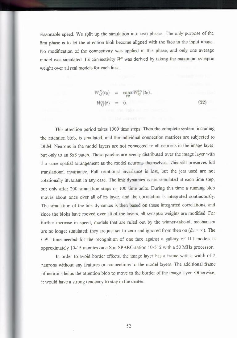
reasonable speed. We split up the simulation into two phases. The only purpose of the

first phase is to let the attention blob become aligned with the face in the input image.

No modification of the connectivity was applied in this phase, and only one average

model was simulated. Its connectivity W was derived by taking the maximum synaptic

weight over all real models for each link:

ı..ı,~a{t· ) - . ,Uf'Pff(J ).rr,1 ,o - ~;x nt, ı.o ,

ff'İj(f) = o. (22)

This attention period takes 1000 time steps. Then the complete system, including

the attention blob, is simulated, and the individual connection matrices are subjected to

DLM. Neurons in the model layers are not connected to all neurons in the image layer,

but only to an 8x8 patch. These patches are evenly distributed over the image layer with

the same spatial arrangement as the model neurons themselves. This still preserves full

translational invariance. Full rotational invariance is lost, but the jets used are not

rotationally invariant in any case. The link dynamics is not simulated at each time step,

but only after 200 simulation steps or 100 time units. During this time a running blob

moves about once over all of its layer, and the correlation is integrated continuously.

The simulation of the link dynamics is then based on these integrated correlations, and

since the blobs have moved over all of the layers, all synaptic weights are modified. For

further increase in speed, models that are ruled out by the winner-take-all mechanism

are no longer simulated; they are just set to zero and ignored from then on (/Jo = oo). The

CPU time needed for the recognition of one face against a gallery of 111 models is

approximately 10-15 minutes on a Sun SPARCstation 10-512 with a 50 MHz processor.

In order to avoid border effects, the image layer has a frame with a width of 2

neurons without any features or connections to the model layers. The additional frame

of neurons helps the attention blob to move to the border of the image layer. Otherwise,

it would have a strong tendency to stay in the center.

52

~

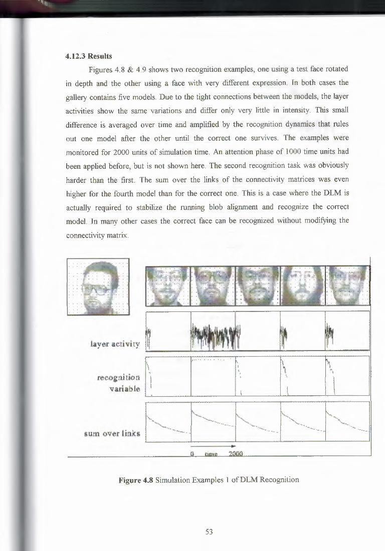
4.12.3 Results Figures 4.8 & 4.9 shows two recognition examples, one using a test face rotated

in depth and the other using a face with very different expression. In both cases the

gallery contains five models. Due to the tight connections between the models, the layer

activities show the same variations and differ only very little in intensity. This small

difference is averaged over time and amplified by the recognition dynamics that rules

out one model after the other until the correct one survives. The examples were

monitored for 2000 units of simulation time. An attention phase of I 000 time units had

been applied before, but is not shown here. The second recognition task was obviously

harder than the first. The sum over the links of the connectivity matrices was even

higher for the fourth model than for the correct one. This is a case where the DLM is

actually required to stabilize the running blob alignment and recognize the correct

model. In many other cases the correct face can be recognized without modifying the

connectivitymatrix.

"-.<,sum over links ı -~..__

layer a,ctivity

ıeeogni tion 1 ·1variable , l

Figure 4.8 Simulation Examples I ofDLM Recognition

53

~ -----·-

layer aetl vi ty II

reeegni tionvariable

sum over Ilnks

·ı-.,«l\'Ilı, t',....•.. ··ı

t'

..,...•.~ ..~-.. ....•......••.....__ ..,_,..,

Figure 4.9 Simulation Examples 2 ofDLM Recognition

The test images are shown on the left with 16x17 neurons indicated by black

dots. The models have lOxlO neurons and are aligned with each other. The respective

total layer activities, i.e., the sum over all neurons of one model, are shown in the upper

graphs. The most similar model is usually slightly more active than the others. On that

basis the models compete against each other, and eventually the correct one survives, as

indicated by the recognition variable. The sum over all links of each connection matrix

is shown in the lower graphs. It gives an impression of the extent to which the matrices

self-organizebefore the recognition decision is made.

Recognition rates for galleries of 20, 50, and ll 1 models are given in Table 4.3. As is

already known from previous work [39], recognition of depth-rotated faces is in general

less reliable than, for instance, recognition of faces with an altered expression (the

examples in Figures 4.8 & 4.9 are not typical in this respect). It is interesting to consider

recognition times. Although they vary significantly, a general tendency is noticeable:

Firstly, more difficult tasks take more time, i.e., recognition time is correlated with error

rate. This is also known from psychophysical experiments. Secondly, incorrect

54

recognition takes much more time than correct recognition. Recognition time does not

depend very much on the size of the gallery.

Table 4.3 Recognition Results Against a Gallery

of 20, 50, and 111 Neutral Frontal Views

Gallery Correct ll,ocog,tıition Time forSize Test Images Rec .• Correct Inoorrectngnıtıon

:# 11.ue % fi - 't' ]lecmmitıon... .:.c: ___ c,,-ll l.00

111 rotatıed faces (15 degrees) 106 95.5, sıo :ı:: 400 5120 ±357:020 110 rot.ated faces (30 degrees) 91 82.1 900 ±1910 4070 ±4810

100 thıntal vie'\\'S (tll'imace) 102 93.6 3HJ ± 420 487() ±6010111 mtat.ed faces (15 degrees) 104. 93.7 370 ± 450 8530±5800

50 110 rotated faces (30 degrees) sa 75.5 · · s-ıo: 140 541 O ::i: 7270109 frontal views (grimace) 95 87.2 440 ±1000 2670 ±1660111 rotated faces {15 degrees) 102 91.9

..

450 ± 100 2fül0 ±2000...

HJ l 10 rotated f34-;es (30 degre,.s) 73 66.4 1180 ±14.'lO 4400±4820llliJ frontal views (grimace) 93 85.3 480 :I: 720 3440±2830

Recognition time (with two iterations of the differential equations per time unit)

ıs the time required until all but one models are ruled out by the winner-take-all

mechanism.

4.13 Discussion The model for visual object recognition we are presenting here marks the

extreme end of a scale, relying minimally on pre-existing structure. In fact, all it needs

is some natural intracortical connection patterns, one stored example for each object to

be recognized, and a simple mechanism of on-line self-organization in the form of rapid

reversible synaptic plasticity. This distinguishes it from many alternative neural models

for object recognition, which require extensive control structures [32] or specific feature

hierarchies, to be created by training [35,40], before the first object can be recognized.

The lateral connections within the image domain and the model domain of our system

encode the a priori constraint of conservation of spatial continuity during the match.

The match itself is realized with the help of the rapid self-organization of the synaptic

connections between image and models. This self-organization is controlled by signal

correlations and by feature similarity between image points and model points. For each

object to be recognized just a single model needs to be stored, which can be done with

the help of simple mechanisms of associative memory [48]. (For the accommodation of

55

~ ~~~~-

substantial rotation in depth the object needs to be inspected from many angles and the

resulting models need to be fused into one model graph. From these properties of our

system results a very clear-cut message concerning the issue of intracortical

connections: visual object recognition can be understood on the basis of simple

connectivity structures and mechanisms of plasticity that are already known today or at

least are well within the reach of existing experimental techniques!

The model leaves open a number of questions regarding the structure of lateral

connections, especially in the model domain. The global interaction between models

could be realized with the help of a single cardinal cell per model, or it could take the

form of a distributed set of connections between model neurons. The anatomy of the

local interaction between models, second term on the right-hand side of Equation 1, can

only be discussed after the relative anatomical placement of different models has

become clear. Also, the extent and the nature of the overlap between models in terms of

common neurons and common connections must be clarified first. Two extreme

versions are imaginable, ( 1) models are laid down in mutual register in terms of internal

position, and (2) there is a fixed spatial array of feature types in infero-temporal cortex,

and laying down a model consists in selecting appropriate feature cells and"connecting

these as required by the inner structure of the model. In the first case, the lateral model

connections would be tidy and local within the cortical tissue (at least their excitatory

part), in the second they would form a diffuse fiber plexus without any apparent

anatomical structure. A further aspect of intracortical connectivity that we are totally

ignoring in the present system concerns intra-hypercolumnar connectivity. This is

implicitly present, being required to organize the necessary feature specificity, and

probably also for the evaluation of the feature similarity between a pair of

hypercolumns(''nodes") in image and model.

Last, and by no means least, we have given short shrift to the issue of inter-areal

organization of connections, by lumping all primary areas into one image domain and

all infero-temporal areas into one model domain. Within the image domain, two

extreme views could be taken. i) The different areas (Vl, V2, V4, for instance)

represent different mixtures of feature specificities and are tied together by rigid

retinotopically organized connections. In that case areal structure could be ignored for

the purposes of our present system, and neurons in different areas but subserving the

same retinal point could just be lumped together into one "hyper-hypercolumn." ii) The

synaptic projection systems between areas are substantially reorganized during the

56

recognition process, areas perhaps forming sequential layers connecting Vl indirectly

with IT. Perhaps such an indirect connectivity scheme can reduce the enormous number

of fibers required by our system for connecting any pair of points in image and models.

There is one apparent mismatch between the system and the reality of object recognition

in the brain of adults: the time taken by the process. There are reports that objects of

different type can be distinguished by human subjects in less than a tenth of a second

[44]. In contrast, our system requires for the process many hundred sequential steps. It

is not easy to interpret these sequential steps in terms of biological real time. The

essential parameter seems, however, to be the temporal resolution with which signal

correlations can be evaluated in our brain. This issue is at present under heated

discussion [42,43], but there is little hope that this resolution is better than one or a few

milliseconds. In this case the hundreds of sequential steps required by our system

translate into many hundred milliseconds, which is unrealistically long. Dynamic Link

Matching needs this time to reduce the enormous ambiguity in the feature similarities

between image and object points to a sparse set of connections between corresponding

points. If this ambiguity could be decisively reduced with the help of highly specific

feature types (which in an extreme case were private to one object type), recognition

time could be cut drastically. The feature types we are using, Gabor-based wavelets, are

very general and unspecific. It is likely that highly specific features can only be

generated by a learning mechanism. It is our view that the basic mechanism of our

system is used by the young animal to store and recognize objects early in its life. At

first, each recognition process may take seconds, but the mechanism can be the basis for

very efficient learning of specific feature types, a process that due to the Dynamic Link

Mechanism is not hampered by confusion between different objects.

4.14 Summary The most encouraging aspect of the system is its evident capability to solve the

invariant object recognition problem in spite of all the difficulties and adversities posed

by real images and in spite of large numbers and great structural overlap of objects to be

distinguished. This puts it in sharp contrast to proposed recognition mechanisms that

work only on simple toy examples. We therefore feel that this system is a foot in the

door, and its remainingdifficultiescan be solved gradually.

57

CHAPTER FIVE

PRINCIPAL COMPONENT

ANALYSIS AND NEURAL NETWORK

5.1 Overview The problem can be described as following. Given an image of human face,

compare it with models in the database and report who it is if a match exists. Here the

image is gray scale, vertically oriented frontal view. Normal expression variation is

allowed and the image is prepared under roughly constant illumination.

Because usually images are bigger than the actual faces, the first problem is to

find the face in the image, or face detection which is another closely related problem.

We use the face detection code by Kah-Kay Sung from MIT Artificial Intelligence Lab.

We make some change to the code to make it run faster and locate face more accurately.

Principal component analysis is applied to find the aspects of face which are important

for identification. Eigenvectors (eigenfaces) are calculated from the initial face image

set. New faces are projected onto the space expanded by eigenfaces and represented by

weighted sum of the eigenfaces. These weights are used to identify the faces.

Neural network is used to create the face database and recognize the face. Each

person have a separate network. The input face is projected onto the eigenface space

first and get a new descriptor. The new descriptor is used as network input and applied

to each person's network. The one with maximum output is selected and reported as the

host if it passes predefined recognition threshold.

Figure 5.1 Face recognition structure

58

5.2 Face Detection

The problem before face recognition is face detection which finds the face in the

image. We use the code from the MIT Artificial Intelligence Lab [52] (below we call it

face detection code ) to locate the face inside the image and cut it out for recognition.

Using the face detection code to prepare the face not only facilitates the recognition

problem, but also set a uniform standard as to which part of the image should be used as

face which can't be achieved through hand segmentation.

The face detection code search the face by exhaustively scanning the image at all

possible scales. Kah-Kay Sun started the face pattern size from 20x20 pixels and

increased it by a scalar (O. 1). In our situation, we search a specific portion of the image

(usually from 40% to 80% ) for the face. It will help to speed the face detection

procedure. If the actual face size is big, linear increase of the face pattern size will lead

to coarse face location. So we increase the face pattern size arithmatically by 4 pixels at

each step to locate the face more accurately.

For each window pattern, a series of 3 templates is applied sequentially to

determine whether the input image is a face. If the output of any test fails to pass the

predefined threshold (usually 0.5), it is rejected immediately. A face is reported only

after the window pattern passes all the tests and the minimum of the 3 test results will

be selected as the final output. In our environment, we can assume that there is no more

than one face in the image. We set the threshold dynamically by replacing it with the

maximum output up to the searching point. This greatly reduces the time cost on

searching by avoiding unnecessary template tests.

If the image contains more than one person, we have to set a predefined

threshold for face finding. For each face inside the image, most of the time the code will

find multiple face templates for it with small location shift and size change. Finally all

the face templates are packed to give only one face for each person in the image.

In our tests, most of the time the face detection code can find the face. It gives higher

outputs on upright face images than those from images with orientation change. But the

objective of the face detection code is to find faces inside images. Its aim is not to cut

faces from images for recognition purpose. We have found that sometimes the face

templates located by the code are smaller than their actual size or not central to the

actual faces.

59

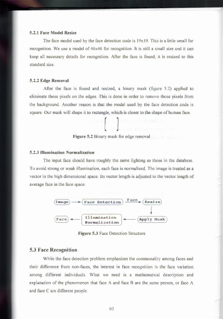
5.2.1 Face Model Resize

The face model used by the face detection code is 19xl9. This is a little small for

recognition. We use a model of 46x46 for recognition. It is still a small size and it can

keep all necessary details for recognition. After the face is found, it is resized to this

standard size.

5.2.2 Edge Removal

After the face is found and resized, a binary mask (figure 5.2) applied to

eliminate those pixels on the edges. This is done in order to remove those pixels from

the background. Another reason is that the model used by the face detection code is

square. Our mask will shape it to rectangle, which is closer to the shape of human face.

[ ]Figure 5.2 Binary mask for edge removal

5.2.3 Illumination Normalization

The input face should have roughly the same lighting as those in the database.

To avoid strong or weak illumination, each face is normalized. The image is treated as a

vector in the high dimensional space. Its vector length is adjusted to the vector length of

average face in the face space.

(I111Age)--+ (Faoe Deteotıon) F~ce ( Reııı.:i.ze)

1ı:ll.um:Lna t.ion

orınaıJ.zat.i.c:m(11pp1y Kask)

Figure 5.3 Face Detection Structure

5.3 Face RecognitionWhile the face detection problem emphasizes the commonality among faces and

their difference from non-faces, the interest in face recognition is the face variation

among different individuals. What we need is a mathematical description and

explanation of the phenomenon that face A and face B are the same person, or face A

and face C are different people.

60

Unlike the face detection where there are only two classes of objects, faces and

non-faces, here each individual is a separate class. All faces have the same facial

features and are basically very similar in overall configuration. It makes the face

recognition a difficult and fine discrimination problem. Another thing which makes it

more complicated is that each individual's face can have many variations because of the

change in orientation, expression and lighting. While we hope that the system could

handle a wide range of variation in real tests, the number of examples in learning a

specific individual's face is always limited.

A face image is a two dimensional array of intensity values. In our experiments

the standard size is 46x46. It can also be treated as a vector or a point in a space of

dimension 2116. But face images are not randomly distributed in this high dimensional

space. The fact that all faces are basically very similar to each other and have the same

facial features such as eyes, nose and mouth makes all the faces a subset of the whole

image space, in other words, the dimension of the face space is smaller than that of the

ımage space.Sirovich and Kirby [54] and Kirby and Sirovich [55] first applied the principal

component analysis in efficient face representation. In this technique a new coordinate

system is created for the faces where coordinates are part of the eigenvectors of a set of

face images. New faces can be approximately reconstructed with only part of their

projection onto the new low-dimensional space.

Matthew Turk and Alex Pentland [51] expanded the idea to face recognition. Faces are

encoded by a small set of weights corresponding to their projection onto the new

coordinate system, and are recognized by comparing them with those of known

individuals.

5.3.1 Eigenspace Representation First we prepare an initial set of face images [Xl, X2, ... , Xn]. The average face

of the whole face distribution isX = (XI + X2 + ... + Xn )/n

Then the average face is removed from each face,Xi'= Xi - X, i = 1, 2, ... , n

The eigenvectors are calculated from the new image set [XI', X2', ... Xn'] as

[Yl, Y2, ... , Yn]. These eigenvectors are orthonormal to each other. They do not

correspond directly to any face features like eyes, nose and mouth. Instead they look

61

like sort of face and are refered as eigenfaces. They are a set of important features

which describe the variation in the face image set. The dimension of the complete

eigenspace is n-I because the eigenvalue of the remaining eigenface is O. Our eigenface

space is created with 593 face images (Figure 5.4).

Figure 5.4 Part Of The Face İmages Used To Create Eigenspacee

As a property to the eigenvector, each of them has an eigenvalue associated with

it. More important, eigenvectors with bigger eigenvalues provide more information on

the face variation than those with smaller eigenvalues. This is in contrast to the

Euclidian space representation where all axes are of the same importance. Figure 5.5

and 5.6 show the eigenfaces with high and low eigenvalues respectively.

62

Figure 5.5 The First 20 Eigenfaces With The Highest Eigenvalues

Figure 5.6 Eigenfaces With Eigenvalues Ranked From 141 To 160

63

-~-~-------~

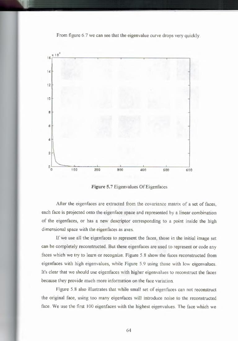
From figure 6.7 we can see that the eigenvalue curve drops very quickly.

-12 .

jQ!r- ~

e

2~\ -

ao HUl zee aeo ,eo 500 600

Figure 5.7 Eigenvalues OfEigenfaces

After the eigenfaces are extracted from the covariance matrix of a set of faces,

each face is projected onto the eigenface space and represented by a linear combination

of the eigenfaces, or has a new descriptor corresponding to a point inside the high

dimensional space with the eigenfaces as axes.

If we use all the eigenfaces to represent the faces, those in the initial image set

can be completely reconstructed. But these eigenfaces are used to represent or code any

faces which we try to learn or recognize. Figure 5.8 show the faces reconstructed from

eigenfaces with high eigenvalues, while Figure 5.9 using those with low eigenvalues.

It's clear that we should use eigenfaces with higher eigenvalues to reconstruct the faces

because they provide much more information on the face variation.

Figure 5.8 also illustrates that while small set of eigenfaces can not reconstruct

the original face, using too many eigenfaces will introduce noise to the reconstructed

face. We use the first 100 eigenfaces with the highest eigenvalues. The face which we

64

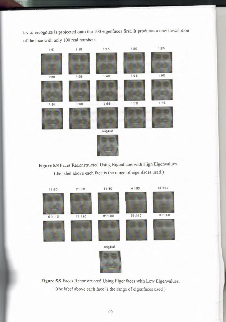
try to recognize is projected onto the 100 eigenfaces first. It produces a new description

of the face with only 100 real numbers.

t:10 1 :i5 1 :20 l :25

Figure 5.8 Faces Reconstructed Using Eigenfaces with High Eigenvalues.

(the label above each face is the range of eigenfaces used.)

11 :60

6Mt0

21 :70

7f:i2G

31:90 41:Sffl

Ot :UQ HH:150

Figure 5.9 Faces Reconstructed Using Eigenfaces with Low Eigenvalues.

(the label above each face is the range of eigenfaces used.)

65

Because projection onto the eigenface space describes the variation of face

distribution, it's natural to use these new descriptors of faces to classify them. Faces are

recognized by comparing the new face descriptor with the face database which has been

encoded in the same way. One approach to find the face pattern is to calculate the

Euclidian distance between the input face descriptor and each known face model in the

database. All faces of the same individual are supposed to be close to each other while

different persons have different face clusters. But actually we don't have any prior

knowledge on the distribution of the new face descriptors. We can't assume it to be

Gaussian distribution and each individual will make one cluster. We have found that

usage of this method is not sufficient in real tests.

A better approach is to recognize the face in unsupervised manner using neural

network architecture. We collect typical faces from each individual, project them onto

the eigenspace and neural networks learn how to classify them with the new face

descriptor as input.

5.3.2 Neural Network

The neural network has a general backpropagation structure with three layers.

The input layer has 100 nodes from the new face descriptors. The hidden layer has 1 O

nodes. The output unit gives a result from O.O to 1.0 telling how much the input face can

be thought as the network's host.

mput wyeı-(100)(New Fa<::€! De;saipt<:<r)

()gtput Unit (D.O - 1.0)

O~o· ·.· ··./.· .o - ~~. · .. . · · · o________-·· .... o:~········· ·.i .. ··o - o

Figure 5.10 Neural Network Structure

In order to make the training of neural network easier, one neural net is created

for each person. Each neural net identifies whether the input face is the network's host

or not. The recognition algorithm selects the network with the maximum output. If the

output of the selected network passes a predefined threshold, it will be reported as the

host of the input face. Otherwise the input face will be rejected.

66

5.3.3 Training Set

After the neural network structure is set, the most important thing is to prepare

the training examples. In the beginning of the training, we select a number of face

images from each person that are well aligned frontal view. Any of them can represent

their host clearly. All the faces here are extracted or cut by the face detection code.

These faces will be used as positive examples for their own networks and negative

examples for other networks.

Here we only deal with images which assume that they are always faces. In our

tests, most of the time the face detection code can find the face if it exists. The database

is not supposed to handle non-face images because in our situation it's unnecessary and

it will make network training very difficult.

After the basic neural networks are created, we run them over new faces from

the individuals in our database. If the image fails to pass the face detection test, it will

be ignored. If the face detection code reports a face in the image, it will be applied to

the face recogniton code. We check the recognition result to find more faces for

training. Here each face will fall into one of the four categories as following:

1. Faces have high output on their own networks and low output on other

networks. No action here.

2. Faces have high output on both their own networks and some other

networks. These faces will be used as negative examples for other

networks.

3. Faces are well-aligned frontal view and clearly represent their hosts.

They have low output on their own networks. These faces will be used as

both positive examples for their own networks and negative examples for

other networks.

4. Faces are not well cut and can't represent their hosts clearly. They have

low output on their own networks. If they have high output on some

67

other networks, they will be included as negative examples for other

networks. Otherwise they will be ignored.

5. Once we get these new faces, we add them to training examples and

retrain the neural networks. Recognition errors will be corrected and the

total performance will be improved. While adding some examples from a

specific individual will improve the performance of his own network, it

will also influence the performance of other networks. In an experiments,

the network training process continues until no significant recognition

errors are found.

5.3.4 Normalize Training Set If we use the original face descriptors from the training examples as neural

network input, it will be difficult to make the network converge. What we do is to make

the average of the training set to zero and unify its standard derivation.

5.4 Summary Neural network is used to create the face database and recognize the face. Each

person has a separate network. The input face is projected onto the eigenface space first

and get a new descriptor. The new descriptor is used as network input and applied to

each person's network. The one with maximum output is selected and reported as the

host if it passes predefined recognition threshold.

68

CONCLUSION

Face recognition is one of the several approaches for recognısıng people.

There are several methods that can be used for that purpose. Some of the most common

are using PCA or eigenfaces. Thought there are other new techniques more simple to

understand use and implement but also with very good performance.

Face recognition technology has come a long way in the last twenty years.

Today, machines are able to automatically verify identity information for secure

transactions, for surveillance and security tasks, and for access control to buildings.

These applications usually work in controlled environments and recognition algorithms

that can take advantage of the environmental constraints to obtain high recognition

accuracy. However, next generation face recognition systems are going to have

widespread application in smart environments, where computers and machines are more

like helpful assistants. A major factor of that evolution is the use of neural networks in

face recognition. A different filed of science that also is very fast becoming more and

more efficient, popular and helpful to other applications.

The combination of these two fields of science manage to achieve the goal of

computers to be able to reliably identify nearby people in a manner that fits naturally

within the pattern of normal human interactions. They must not require special

interactions and must conform to human intuitions about when recognition is likely.

This implies that future smart environments should use the same modalities as humans,

and have approximately the same limitations. These goals now appear in reach

however, substantial research remains to be done in making person recognition

technology work reliably, in widely varying conditions using information from single or

multiple modalities.The important of Face Recognition is shown with many application in which the

face recognition is approached, using an eigenfaces demo we described the work of an

automatic system for detection, recognition and coding. Also we described how we can

perform a Face Recognition system by Dynamic Link Matching which involve the blob

formation and mobilization, and also the link, attention and recognition dynamics. By

performing a training set for Neural Network face recognition is realized.

69

.

The capability of the dynamic link matching to solve the invariant object

recognition problem is proofed and the efficiency of the neural network application is

analyzed and maintained.

70

REFERENCES

[1] web page http://www-white.media.mit.edu/tech-reports/TR-516/node3.html.

[2] web page http://www-white.media.mit.edu/tech-reports/TR-516/node5.html.

[3] R.Chellappa, C.L.Wilson, andS.Sirohey, Human and Machine Recognition of Faces:

A Survey, Proceedings of the IEEE, 83(5), 1995.[4] M. Kirby and L. Sirovich, "Application of the karhunen-loeve procedure for the

characterization of human faces, " IEEE Pattern Analysis and Machine Intelligence,

vol. 12, no. 1, pp. 103-108, 1990.[5] T. Kanade, "Picture Processing by Computer Complex and Recognition of Human

Faces", PhD thesis, Kyoto University, 1973.[6] R. Brunelli and T. Poggio, Face recognition: Features versus templates, IEEE

Transactions on Pattern Analysis and Machine Intelligence, 15(1O):1042-1052,October

1993.[7] Ingemar J. Cox, Joumana Ghosn, and Peter N. Yianilos, Feature-based face

recognition using mixture-distance, In Computer Vision and Pattern Recognition. IEEE

Press, 1996.[8] K. Sutherland, D. Renshaw, and P.B. Denyer, Automatic face recognition, In First

International Conference on Intelligent Systems Engineering, pages 29-34, Piscataway,

NJ, 1992. IEEE Press.[9] D. Marr, Vision., W. H. Freeman, San Francisco, 1982.[10] M. Turk and A. Pentland, Eigenfaces for recognition, J of Cognitive Neuroscience,

3:71-86, 1991.[1 l]Perret, Rolls, and Caan,Visual neurones responsive to faces in the monkey temporal

cortex, Experimental Brain Research, 47:329-342, 1982.[12] A. Pentland, T. Starner, N. Etcoff, A. Masoiu, O. Oliyide, and M. Turk,

Experiments with eigenfaces,In Looking at People Workshop, International Joint

Conference on Artificial Intelligence 1993, Chamberry, France, 1993.

[13] A. Pentland, B. Moghaddam, and T. Starner, View-based and modular eigenspaces

for face recognition, In IEEE Conference on Computer Vision and Pattern Recognition,

1994.[14] B. Moghaddam and A. Pentland, Face recognition using view-based and modular

eigenspaces, In Automatic Systems for the Identification and Inspection of Humans,

SP IE, volume 2257, 1994.

71

[15] D.L. Swets and J.J. Weng, Using discriminant eigenfeatures for image retrieval,

IEEE Transactions on Pattern Analysis and Machine Intelligence, to appear, 1996.

[16] Martin Lades, Jan C. Vorbrüggen, Joachim Buhmann, Jörg Lange, Christoph von

der Malsburg, Rolf P. Würtz, and Wolfgang Konen, Distortion invariant object

recognition in the dynamic link architecture, IEEE Transactions on Computers,

42(3):300-311, 1993.[17] Laurenz Wiskott, Jean-Marc Fellous, Norbert Krüger, and Christoph von der

Malsburg, Face recognition and gender determination, In Proceedings of the

International Workshop on Automatic Face and Gesture Recognition, Zürich, 1995.

[18] David DeMers and G.W. Cottrell, Non-linear dimensionality reduction, In S.J.

Hanson, J.D. Cowan, and C. Lee Giles, editors, Advances in Neural Information

Processing Systems 5, pages 580-587, San Mateo, CA, 1993. Morgan Kaufmann

Publishers.[19] J. Weng, N. Ahuja, and T.S. Huang, Learning recognition and segmentation of 3-d

objects from 2-d images, In Proceedings of the International Conference on Computer

Vision, ICCV93, pages 121-128, 1993.[20] F.S. Samaria and A.C. Harter, Parameterisation of a stochastic model for human

face identification, In Proceedings of the 2nd IEEE workshop on Applications of

Computer Vision, Sarasota, Florida, 1994.[21] F.S. Samaria, Face Recognition using Hidden Markov Models, PhD thesis, Trinity

College, University of Cambridge, Cambridge, 1994.[22] K. Fukunaga, Introduction to Statistical Pattern Recognition, Second Edition,

Academic Press, Boston, MA, 1990.[23] Y. Le Cun and Yoshua Bengio, Convolutional networks for images, speech, and

time series, In Michael A. Arbib, editor, The Handbook of Brain Theory and Neural

Networks, pages 255-258. MIT Press, Cambridge, Massachusetts, 1995.

[24] Y. Le Cun, B. Boser, J.S. Denker, D. Henderson, R. Howard, W. Hubbard, and L.

Jackel, Handwritten digit recognition with a backpropagation neural network, In D.

Touretzky, editor, Advances in Neural Information Processing Systems 2, pages 396-

404. Morgan Kaufmann, San Mateo, CA, 1990.[25] Y. Le Cun, Generalisation and network design strategies, Technical Report CRG-

TR-89-4, Department of Computer Science, University of Toronto, 1989.

[26] L. Bottou, C. Cortes, J.S. Denker, H. Drucker, I. Guyon, L. Jackel, Y. Le Cun, U.

Muller, E. Sackinger, P. Simard, and V.N. Vapnik, Comparison of classifier methods: A

72

case study in handwritten digit recognition, In Proceedings of the International

Conference on Pattern Recognition, Los Alamitos, CA, 1994. IEEE Computer Society

Press.[27] Yoshua Bengio, Y. Le Cun, and D. Henderson, Globally trained handwritten word

recognizer using spatial representation, space displacement neural networks and hidden

Markov models,In Advances in Neural Information Processing Systems 6, San Mateo

CA, 1994. Morgan Kaufmann.

[28] D.H. Hubel and T.N. Wiesel, Receptive fields, binocular interaction, and functional

architecture in the cat's visual cortex, Journal of Physiology (London), 160:106-154,

1962.

[29] S. Haykin, Neural Networks, A Comprehensive Foundation, Macmillan, New

York, NY, 1994.

[30] web page http://www.white.media.mit.edu/vismod/demos/facerec.

[31 J S. Amari. Dynamics of pattern formation in lateral-inhibition type neural fields.

Biological Cybernetics, 27:77--87, 1977.

[32] C. H. Anderson and C. V. van Essen. Shifter circuits: A computational strategy for

dynamic aspects of visual processing. Proceedings of the National Academy of Sciences

USA, 84:6297--6301, 1987.

[33] V. Bruce, T. Valentine, and A. Baddeley. The basis of the 3/4 view advantage in

face recognition. Applied Cognitive Psychology, 1: 109--120, 1987.

[34] M. Eigen. The hypercycle.Naturwissenschaften, 65:7--41, 1978.

[35] K. Fukushima, S. Miyake, and T. Ito. Neocognitron: A neural network model for a

mechanism of visual pattern recognition. IEEE Transactions on Systems, Man, and

Cybernetics, 13:826--834. Also appeared in J. A. Anderson and E. Rosenfeld, editors,

Neurocomputing, 526--534, MIT Press, Cambridge, MA, 1983.

[36] P. Kalocsai, I. Biederman, and E. E. Cooper. To what extent can the recognition of

unfamiliar faces be accounted for by a representation of the direct output of simple

cells. In Proceedings of the Association for Research in Vision and Ophtalmology,

ARVO, Sarasota, Florida, 1994.

[37] W. Konen, T. Maurer, and C. von der Malsburg. A fast dynamic link matching

algorithm for invariant pattern recognition.Neural Networks, 7:1019--1030, 1994.

[38] W. Konen and J. C. Vorbrüggen. Applying dynamic link matching to object

recognition in real world images. S. Gielen and B. Kappen, editors, Proceedings of the

73

International Conference on Artificial Neural Networks, !CANN, 982--985, London.

Springer-Verlag, 1993. [39] M. Lades, J. C. Vorbrüggen, J. Buhmann, J. Lange C. von der Malsburg, R. P.

Würtz, and W. Konen. Distortion invariant object recognition in the dynamic link

architecture. IEEE Transactions on Computers, 42(3):300--311, 1993.

[40] Y. LeCun, B. Boser, J. Denker, D. Henderson, R. Howard, W. Hubbard, and L.

Jackel. Backpropagation applied to handwritten zip code recognition. Neural

Computation, 1(4):541--551, 1989. [ 41] K. Reiser. Learning persistent structure. Doctoral thesis, res. report 584, Hughes

Aircraft Co., 3011 Malibu Canyon Rd. Malibu, CA 90265, 1991.

[42] M. N. Shadlen and W. T. Newsome. Is there a signal in the noise? Current Opinion

in Neurobiology, 5:248--250, 1995. [ 43] W. Softky. Simple codes vs. efficient codes. Current Opinion in Neurobiology,

5:239--247, 1995. [44] S. Subramaniam, I. Biederman, P. Kalocsai, and S. Madigan. Accurate

identification, but chance forced-choice recognition for rsvp pictures. In Proceedings of

the Association for Research in Vision and Ophtalmology, AR VO, Ft. Lauderdale,

Florida, 199 5. [45] K. Tanaka. Neuronal mechanisms of object recogntition. Science, 262:685--688,

1993. [ 46] C. von der Malsburg. The correlation theory of brain function. Internal report, 81-

2, Max-Planck-Institut für Biophysikalische Chemie, Postfach 2841, 3400 Göttingen,

FRG, 1981. [47] C. von der Malsburg. Nervous structures with dynamical links. Ber. Bunsenges.

Phys. Chem., 89:703--710, 1985. [ 48] C. von der Malsburg. Pattern recognition by labeled graph matching. Neural

Networks, 7:1019--1030, 1988. [ 49] L. Wiskott. Labeled Graphs and Dynamic Link Matching for Face Recognition

and Scene Analysis. PhD thesis, Fakultat für Physik und Astronomie, Ruhr-Universitat

Bochum, D-44780 Bochum, 1995. [50] L. Wiskott, J.-M. Fellous, N. Krüger, and C. von der Malsburg. Face recognition

and gender determination. In Proceedings of the International Workshop on Automatic

Face- and Gesture-Recognition, IWAFGR 95, 92--97, Zurich, 1995.

74

[51] M. Turk and A. Pentland, "Eigenfaces for recognition", Journal of Cognitive

Neuroscience, vol. 3, no. 1, pp.71-86, 1991

[52] K. Sung and T. Poggio, "Example-based learning for view-based human face

detection", A.I. Memo No.1521, Artificial Intelligence Laboratory, Massachusetts

Institute of Technology, 1994 [53] Henry A. Rowley, Shumeet Baluja and Takeo Kanade, "Human face detection in

visual scenes", CMU-CS-95-158R, Carnegie Mellon University, November 1995

[54] Roberto Brunelli and Tomaso Poggio, "Face recognition: feature versus

templates", IEEE Transactions on Pattern Analysis and Machine Intelligence,

15(1O):1042-1052, 1993 [55] L. Sirovich and M. Kirby, "Low-dimensional procedure for the characterization of

human faces", Journal of the Optical Society of America A, 4(3 ), 519-524, 1987

75