NCGIANational Center for Geographic

Information and Analysis

Two Papers on TriangulatedSurface Modeling

by:

Carlos Felgueiras

Divisao de Processamento de Imagens (DPI)Instituto Nacional de Pesquisas Espaciais (INPE)

Sfio Jose dos Campos, Sao Paulo, Brazil

and

Michael F. Goodchild

University of California, Santa Barbara

Technical Report 95-2

January 1995

Simonett Center for Spatial Analysis State University of New York University of MaineUniversity of California 301 Wilkeson Quad, Box 610023 348 Boardman Hall35 10 Phelps Hall Buffalo NY 14261-0001 Orono ME 04469-5711Santa Barbara, CA 93106-4060 Office (716) 645-2545 Office (207) 581-2149Office (805) 893-8224 Fax (716) 645-5957 Fax (207) 581-2206Fax (805) 893-8617 ncgia@ubvms.cc.buffalo.edu ncgia@spatial.maine.eduncgia@ncgia.ucsb.edu

1

Title:

A COMPARISON OF THREE TIN SURFACE MODELING METHODS AND

ASSOCIATED ALGORITHMS

Authors and affiliations:

CARLOS A. FELGUEIRAS

Divisão de Processamento de Imagens (DPI), Instituto Nacional de Pesquisas Espaciais

(INPE), São José dos Campos, São Paulo, Brazil.

MICHAEL F. GOODCHILD

National Center for Geographic Information and Analysis (NCGIA), Geography Department

University of California Santa Barbara (UCSB), California, USA.

Keywords:

triangulation, interpolation, surface fitting, digital terrain model, fractal.

Short title :

A comparison of three TIN surface modeling methods.

Name and address of the author for correspondence:

Carlos A. Felgueiras

DPI - INPE (Instituto Nacional de Pesquisas Espaciais)

Av. dos Astronautas 1758 - Jardim da Granja - São José dos Campos - SP

CEP 12227 010 - C.P. 515 - São Paulo - Brasil

Fone: 011 55 123 418977 ext 372

Fax: 011 55 123 21 87 43

E-mail: carlos@dpi.inpe.br

Acknowledgments:

We want to express our gratitude to Uwe Deichmann and Julio C. L. D’Alge for helpful

suggestions. We also would like to thank Jonathan Gottesegen and Darrel Lamb for their useful

remarks and comments on earlier drafts of this paper. This work was performed while the first

author was at the National Center for Geographic Information and Analysis (NCGIA) at the

University of California Santa Barbara.

2

A comparison of three TIN surface modeling methods and associated algorithms

Abstract. This paper describes the implementation of three methods for fitting

surfaces: linear, quintic and stochastic. It uses qualitative (visual) and quantitative

(statistical) criteria to compare the three approaches. The digital terrain model is

based on a triangular irregular network (TIN) structure and the comparison is

performed using a mathematically defined function and real data obtained from a

raster digital elevation model (DEM) from a United States Geological Survey

(USGS) elevation file.

1. Introduction

Digital surface representation from a set of three-dimensional samples is an important issue of

computer graphics that has applications in different areas of study such as engineering, geology,

geography, meteorology, medicine, etc. The digital model allows important information to be

stored and analyzed without the necessity of working directly with the real surface. In addition,

we can integrate products from Digital Terrain Model (DTM ) manipulation with other data in a

Geographical Information System (GIS) environment. MacCullagh (1988) presents a detailed

study of DTMs, considering their merge with image processing and database systems.

The main objective of this work is the comparison of different methodologies to model

surfaces from a set of scattered three dimensional samples. The basic structure used to represent

the surface is the triangular irregular network, whose triangle vertices are the sample points.

Another goal of the work is the evaluation of the relative precision of digital models for

representing spatial variation as exactly as possible.

3

This work presents three methods for triangular surface fitting: linear, quintic and stochastic.

It also gives a qualitative (visual) and a quantitative (statistical) analysis of the three methods

using both a mathematically defined function and digital elevation model data, hereafter called

DEM-USGS, as supplied by the United States Geological Survey.

Section 2 introduces the basic concepts related to surface fitting for TIN model structures.

Section 3 describes the methodology used to compare the surface fitting interpolators. Section 4

shows and analyzes the results achieved using the proposed methodology. Section 5 presents the

conclusions and some suggestions for future research related to this work.

2. Triangular Irregular Networks

This work compares the accuracy of different algorithms to fit surfaces for TIN models. De

Floriani (1992), Falcidieno (1993) and Tsai (1993) are recent contribuitions to the vast literature

on the study and implementation of DTMs based on TIN structures. In this section we present

only the principal characteristics of TIN models.

A TIN represents a surface as a set of non-overlapping contiguous triangular facets, of

irregular size and shape (Chen 1987). TIN uses the data on the irregularly spaced samples as the

basis of a system of triangulation (Burrough 1986). It is created directly from the set of samples, i.

e. the vertices of the triangles are the samples. Commonly a TIN is constructed using the

bidimensional projection of the sample points in the xy plane. When the sample set is too dense, it

is necessary to apply an algorithm that chooses a subset, the very important points (VIP ), that

better represents the original surface. This approach reduces the number of points used to create

the TIN model. Lee (1991) performs a comparison of 3 algorithms to reduce the number of points

4

to construct TIN models from rectangular grid DEMs. In some cases, as when the samples are

contour lines, it is imperative to use algorithms for cartographic generalization.

The most popular TIN model, used in commercial software, is the Delaunay TIN. The

Delaunay triangulation is the straight-line dual of the Voronoi diagram and is constructed by

connecting the points whose associated Voronoi polygons share a common edge. The Delaunay

TIN has the following properties:

• It is unique and;

• It maximizes the minimum internal angles of each triangle, i. e. the minimum angle of its

triangles is maximum over all triangulations. This characteristic avoids the creation of thin

triangles, i. e. each triangle is as equilateral as possible.

The circumference that passes through the three vertices of a Delaunay triangle does not

contain any other sample point. This property is known as the empty circle criterion (Tsai 1993).

This property is used to construct the TIN model directly from the sample set. Figure 1 illustrates

the use of the empty circle criterion condition to determine whether a triangle is Delaunay or not.

Another interesting triangular model is the greedy TIN. This network is constructed with

triangles that have the shortest possible edges. Greedy triangulation has been used to hasten the

task to find the nearest neighborhood of a sample point. Preparata (1988) describes some methods

to create greedy triangulations.

2.1. Fitting surfaces for TIN models

In this work we are interested in DTMs whose basic structures are triangular networks. Each

basic element of the TIN, a triangle, can be described by a local polynomial surface whose

parameters depend on its own vertices and, usually, on its triangular neighborhood. This section

5

will discuss three different approaches to interpolate TIN models: linear, quintic and stochastic

triangular surface fitting.

2.1.1. Linear fitting

Each triangle of the TIN model defines a plane that is used to determine the z value of every

point (x, y) inside the triangle. The equation of a plane surface can be expressed as:

Ax + By + Cz + D = 0; (1)

To calculate the coefficients A, B, C and D of the equation 1 it is enough to use the z value

of the 3 vertices of the triangle. Suppose that the three vertices of the triangle have the

coordinates: (x1, y1, z1), (x2, y2, z2) and (x3, y3, z3). These three points define the following linear

equation system:

(A/D)xi + (B/D)yi + (C/D)zi = -1; where i = 1,2,3 (2)

6

The solution of this system, using Cramer's rule for example, gives:

A = y1 (z2 - z3) + y2(z3 - z1) + y3(z1 - z2); (3)B = z1 (x2 - x3) + z2(x3 - x1) + z3(x1 - x2); (4)C = x1 (y2 - y3) + x2(y3 - y1) + x3(y1 - y2) and; (5)D = -x1 (y2z3 - y3z2) - x2(y3z1 - y1z3) - x3 (y1z2 - y2z1); (6)

This linear approach guarantees that the planar surfaces match along the common side of two

adjacent triangles, i. e. the surface has no cliffs. This means that the resulting surface has zero-

order continuity only. The surface has undefined tangents along triangle edges and sharp changes

of slope. To get a higher order continuity along the edges of the adjacent triangular surfaces, it is

necessary to use polynomials of order greater than 1.

2.1.2. Smooth fitting

Akima (1975 and 1978) presents a method of bivariate interpolation and smooth surface

fitting that is applicable to z values given at irregularly distributed samples in the xy plane. Akima

proposed a method based on local procedures. The resulting surface passes through all the given

samples and has continuity of order 2, i. e. slopes and curvatures change smoothly, even across

triangle edges. In sum, it is an algorithm to smoothly fit surfaces over every basic element of a

triangular mesh. A more detailed study of smoothness and derivatives can be found in Lancaster

(1986).

Akima proposed to fit a quintic polynomial function for each triangle. He used the following

fifth-degree polynomial in x and y to evaluate the function at any point (x, y) inside the triangle:

z x y ijq ix jyj

i

i( , ) == ∑∑∑∑

==

−−

== 0

5

0

5

(7)

7

To determine the 21 coefficients qij , in order to solve the equation 7, one has to use the

information from the 3 vertex points ( p1= (x1, y1, z1), p2=(x2, y2, z2) and p3=(x3, y3, z3) ) of the

triangle and their neighbors. For these vertices one must obtain:

• • The z values of the vertex points:

z1, z2 and z3;

• • The first order partial derivatives:

∂∂∂∂

∂∂∂∂

∂∂∂∂

∂∂∂∂

∂∂∂∂

∂∂∂∂== == == == == ==

zx

zx

zx

zy

zy

andzyp p p p p p p p p p p p1 2 3 1 2 3

, , , , ;

• • The second order partial derivatives:

∂∂∂∂

∂∂∂∂

∂∂∂∂

∂∂∂∂

∂∂∂∂

∂∂∂∂

∂∂∂∂

∂∂∂∂

∂∂∂∂

== == == == == == == == ==

2

21

2

22

2

23

2

21

2

22

2

23

2

1

2

2

2

3

z

x

z

x

z

x

z

y

z

y

z

y

zxy

zxy

zxy

p p p p p p p p p p p p p p p p p p

, , , , , , , , ;

• • The partial derivative of the function differentiated in the normal direction to each side,

n⊥⊥s, of the triangle. This is a polynomial of degree three, at most, in the variable

measured in the direction of the side of the triangle (Akima 1978). These assumptions

yield 3 additional conditions related to the three sides of the triangle:

∂∂∂∂

∂∂∂∂

∂∂∂∂⊥⊥ ⊥⊥ ⊥⊥

zn

zn

andznn s n s n s1 2 3

, .

To calculate the partial derivatives in every data point Pk (k=1,2,3,...n; where n is the total

number of data points) one has to use the point itself and its nc closest neighbors. Akima suggests

a number among 3 and 5 for nc.

The evaluation of the partial derivative on a given data point Pk begins with the determination

of the vector normal to the surface at this point. This vector is calculated by performing the

summation of the vectors obtained from the vector product of every pair of vectors formed by Pk

8

and two different neighbors points. The vector product of Pk = (xk, yk, zk) and two of its

neighborhood, Pi = (xi, yi, zi) and Pj = (xj, yj, zj) ιι ≠≠ ϕϕ, can be evaluated by the following

equations:

dzikj = (xi - xk)(yj - yk) - (yi - yk)(xj - xk) (8)

dxikj = (yi - yk)(zj - zk) - (zi - zk)(yj - yk) (9)

dyikj = (zi - zk)(xj - xk) - (xi - xk)(zj - zk) (10)

where dzikj , dxikj and dyikj are the three components of the vector product.

If dzikj < 0 it is necessary to multiply the elements dzikj , dxikj and dyikj by -1 to assure that the

direction of the vector normal to the surface is positive. To calculate the gradient vector, in the x

and y directions, it is necessary to solve the following equations:

∂∂∂∂

== ∑∑∑∑ ∑∑∑∑== == ++

−−

==

−−

== ++

−−

==

−−zx

dx dzp pk

ikjj i

nc

i

nc

ikjj i

nc

i

nc

1

1

0

2

1

1

0

2 (11)

∂∂∂∂

== ∑∑∑∑ ∑∑∑∑== == ++

−−

==

−−

== ++

−−

==

−−zy

dy dzp pk

ikjj i

nc

i

nc

ikjj i

nc

i

nc

1

1

0

2

1

1

0

2 (12)

where dzikj , dxikj and dyikj are evaluated by equations 8, 9 and 10 respectively.

A similar approach can be used to calculate the second derivatives. In this case the

coordinates xi, yi and zi are substituted by ∂∂∂∂

∂∂∂∂== ==

zx

zyp pi p pi

, and 1 in equations 8, 9 and 10.

2.1.3. Stochastic fitting

The most popular stochastic models to represent curves and surfaces are based on fractal

concepts. A fractal is a geometrical or physical structure having an irregular or fragmented

9

shape at all scales of measurement. In addition, a fractal is self-similar meaning that each part of

its structure is similar to the whole.

Smoothed curves and surfaces are subjects of Euclidean geometry, and are adequate to

represent artificial shapes like parts of mechanical and aeronautical projects, furniture, toys, etc..

Natural objects like clouds, coastlines and mountains have irregular or fragmented features.

These are better represented by the Fractal geometry that was first formalized by Mandelbrot

(1982).

Natural phenomena are not exactly self-similar, but statistically self-similar, i. e. each part of

the structure is statistically (averages and standard deviations) similar to the whole. Indeed, real

objects often look similar to pieces of themselves when examined at different cartographic scales

and have forms that manifest significant randomness. Polidori (1991), Finlay (1993) and Fournier

(1982) deal with the description of terrain as a fractal surface.

Fractal dimension (D) is an index that measures the complexity or irregularity of a graphic

object (curve, surface, etc.) that represents a phenomenon. The fractal dimension of a line can be

determined by the relation:

D = log (ni /nj) / log (sj /si) (13)

where: si and sj are two different step sizes used to measure the length of a line and;

ni and nj are the number of si and sj steps to span the line respectively.

Lam (1993) presents some measurement methods to evaluate the fractal dimension for curves

and surfaces.

Brownian motion is the most popular model used to perform fractal interpolations from a

set of samples. Brownian motion, first observed by Robert Brown in 1827, is the motion of small

10

particles caused by continual bombardment by other neighboring particles. Brown found that the

distribution of the particle position is always Gaussian with a variance dependent only on the

length of the time of the movement observation (Finlay 1993).

The Fractional Brownian motion (fBm), derived from Brownian motion, can be used to

simulate topographic surfaces. fBm provides a method of generating irregular, self-similar

surfaces that resemble topography and that have a known fractional dimension (Goodchild 1987).

The fBm functions can be characterized by variograms (graphic that plots the phenomenon

variation against the spatial distance between two points) of the form:

E[(zi - zj)]2 = K*(d ij )

2H (14)

where E denotes the statistical expectation, zi and zj represent the heights of the surface at the

points i and j and dij is the spatial distance between these points. K is a constant of

proportionality and is related to a vertical scale factor S that controls the roughness of the surface.

H is a parameter in the range 0 to 1. H describes the relative smoothness at different scales and

has the following relation with the fractal dimension D:

D = 3 - H (15)

When H is .5 we get the pure Brownian motion. The smaller H, the larger D and the more

irregular is the surface. On the contrary, the larger H, the smaller D and the smoother the surface

(Goodchild 1980).

Fournier (1982) presents recursive procedures to render curves and surfaces based on

stochastic models. He describes two methods to construct two-dimensional fractal surface

primitives. The first one is based on a subdivision of polygons to create fractal polygons while the

second approach is based on the definition of stochastic parametric surfaces.

11

The subdivision of polygons is based on the fractal polyline subdivision method. A fractal

polyline subdivision is a recursive procedure that interpolates intermediate points of a polyline.

The algorithm recursively subdivides the closest extreme intervals and generates a scalar value at

the midpoint which is proportional to the current standard deviation σσc times the scale or

roughness factor S. So, the zm value of the middle point between two consecutive points, i and j,

of a polyline is determined by the following equation:

zm = (zi + zj)/2 + S*σσc *N(0,1) (16)

where σσc varies according to equation 14 and N(0,1) is a Gaussian random variable with zero

mean and unit variance. Press (1988) presents some algorithms to calculate random numbers with

different distributions including the Gaussian.

The subdivision of polygons method is suitable to create stochastic surfaces based on TIN

digital models. Each triangle of the TIN model can be subdivided into four smaller triangles by

connecting the midpoints of the triangles. The z value of the midpoints is calculated by the fractal

polyline subdivision method presented above. The subdivision can be continued until the area or a

side of the current triangle reaches a predefined limit. So the original triangle is transformed into a

fractal triangle whose irregular surface consists of many small triangular facets. Some care must

be taken to ensure internal and external consistency among the adjacent triangles during the

construction of the stochastic TIN model.

As pointed out by Fournier, the presented methods for rendering curves and surfaces are

satisfactory approximations of fractional Brownian motion. They allow us to create realistic

surfaces in faster time than with exact calculations. Another advantage of these approaches is the

possibility of computing surfaces to arbitrary levels of detail without increasing the database.

12

Figure 2 illustrates the behavior of fractal curves created using fractional Brownian motion,

different values of H, and a constant vertical scale factor. The curves were rendered using the

fractal polyline subdivision method.

3. Methodology

This section describes the methodology used to analyze and to compare the different

approaches for surface fitting on TIN models.

We can divide the methodology into five steps:

1. Definition of the input sample set;

2. Construction of a TIN model;

13

3. Surface fitting for a mathematically defined function;

4. Surface fitting for a DEM-USGS data file and;

5. Statistical analysis for rectangular regular grid models.

3.1. Definition of the input sample set

The first step for modeling surfaces is the definition of the input sample set that will be used

to construct the surface. This sample set must be representative of the phenomenon to be

modeled.

To compare the two initial approaches for surface fitting, linear and quintic, we chose two

different patterns. The first pattern of comparison was the following mathematically defined

function that will be called the sinc function hereafter:

z(x, y) = sinc(di) = sin(di)/di (17)

The parameter di in equation 17 means the bi-dimensional euclidean distance from a generic

point Pi (xi, yi) to the point origin P0(0., 0.) , that is, the di parameter is defined by the equation:

di2 = xi

2 + yi2 (18)

This is an interesting test function because it has continuity of degree greater than 0, i. e. is a

smooth function, and has intrinsic positive and negative derivatives.

A DEM-USGS data file was used as the second pattern to evaluate the results with real

elevation data. In this case the stochastic approach was included in the analysis because of the

characteristics of the data and the interpolator.

The sample set was defined by choosing the very important points (VIP ) from rectangular

regular grids obtained from the sinc function and from the DEM-USGS data file. To get the very

14

important sample points from a rectangular regular grid, a variation of the algorithm proposed by

Chen (1987) was used. His method is based on a numerical evaluation of the importance of each

element of the rectangular grid. The algorithm assumes that the greater the elevation difference

between the sample point and its 8 neighbors, the more important it is.

The Chen algorithm was improved by giving a high value, greater than the maximum

possible, to the local maximum or minimum grid points. This assumption guarantees that all peaks

and pits, including the small ones, will be included among the very important points.

3.2. TIN model construction

The next step involves the use of the sample set to construct the basic structure of the DTM

model. Here the input samples were transformed on the vertices of the triangles of a TIN model.

Some important characteristics of the TIN algorithm implemented are:

• It is an incremental algorithm, i. e. the sample points are introduced, one at a time, into

the previous triangulation which is then refined;

• It creates a Delaunay triangulation;

• It uses the Delaunay empty circle criterion locally during the incremental process in order

to avoid local thin triangles and;

• It uses a recursive function to create the final Delaunay triangulation.

Figure 3 depicts six Delaunay triangulations constructed from 93, 253, 505, 757, 997, and

2017 input samples. These input points were defined by the algorithm that chose the very

important points from a rectangular regular grid. The z value for each point of the grid was

obtained from the sinc function.

15

3.3. Surface fitting for mathematical function data

The linear and quintic interpolation approaches were implemented following the concepts

presented in sections 2.1.1 and 2.1.2 respectively. The linear approach depends only on the

vertices of the triangle and is straightforward. To implement the quintic approach two important

details of implementation can be noted here:

• The derivatives at the vertices of the triangles were evaluated and stored during the

quintic interpolation fitting. This avoided the unnecessary calculation of derivatives at the

vertices of triangles that were not used during the process of rectangular grid creation.

• • To evaluate the derivative in the vertices of a chosen triangle it was necessary to find the

neighborhood of each vertex point that formed the triangle. This was accomplished using

the vertices of the triangles that were neighbors of the chosen triangle.

The linear and quintic interpolation functions were compared using the sinc function. To

perform this task rectangular grids (50 x 50 points) were constructed using z values calculated

from the sinc function, from the linear interpolation and from the quintic interpolation. In addition,

two more grids were created representing the difference between the linear and the original

surface, and the quintic and the original surface.

Figures 4 and 5 show the perspective view of rectangular grids fitted by linear and Akima

methodologies. They also show the difference between those models and the model defined by the

sinc function.

16

17

18

19

3.4. Surface fitting for DEM-USGS data

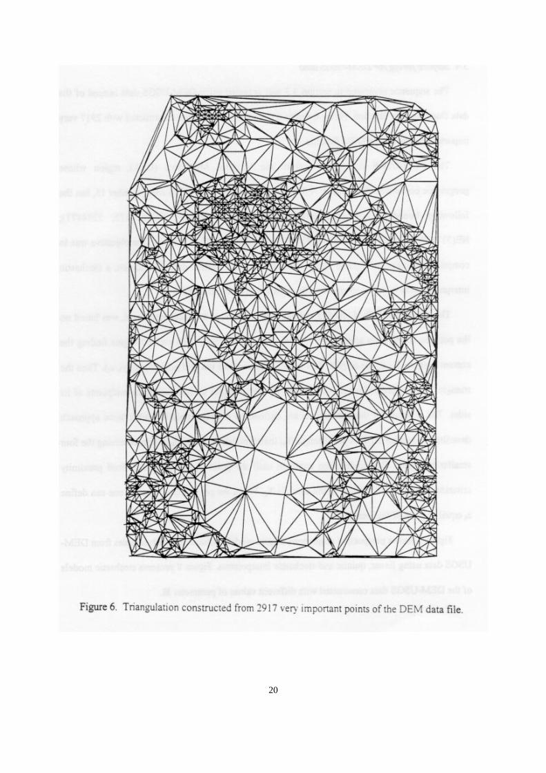
The sequence presented in section 3.3 was repeated using DEM-USGS data instead of the

data from the sinc function. Figure 6 shows a Delaunay triangulation constructed with 2917 very

important points from a DEM data file.

The DEM-USGS data used is from the Virginia, Minnesota (USA), region whose geographic

coordinate reference is: N 43o30’ and W 92o30’. The UTM zone, number 15, has the following

bounding box planimetric coordinates (in meters): NW(528175, 5274471); NE(537568,

5274524); SW(528242, 5260579) and; SE(537658, 5260632). The objective was to compare the

linear and quintic interpolators using real elevation data. In addition, a stochastic interpolator was

included to create surfaces with more natural looks.

The stochastic method, used to estimate the z values of the rectangular grid, was based on

the polygon subdivision approach presented in Fournier (1982). The method begins finding the

current triangle Tc, of the original TIN model, that contains the grid point Pi (xi, yi, zi). Then the

triangle Tc is subdivided recursively in four smaller triangles by connecting the midpoints of its

sides. The z values of these midpoints are defined by a fractal polyline subdivision approach

described in section 2.1.3. A new triangle Tc, that contains the point Pi, is chosen among the four

smaller triangles. The subdivisions continue until the point Pi is within a defined proximity

criterion of one of the vertices of the triangle Tc. When the proximity is reached one can define zi

equal to the z of this vertex.

Figure 7 shows perspective projections of grid models constructed with samples from DEM-

USGS data using linear, quintic and stochastic interpolators. Figure 8 presents stochastic models

of the DEM-USGS data constructed with different values of parameter H.

20

21

22

23

3.5. Statistical analysis of the grid models

In order to perform a quantitative analysis of the surfaces rendered by the three interpolator

approaches, we compared them with the real, or original, surfaces. This was achieved by

comparing the regular rectangular grids created by the interpolators with the real grids.

For each point of a regular rectangular grid we can calculate the error function Er defined as

the difference between the real elevation zr and the estimated elevation ze in that point. The Er

function is defined as:

Er = zr - ze (19)

Suppose that we have npt points representing the surface. To evaluate the average (Av),

variance (Var ) and standard deviation (Std) of the error function (Er ) we can use the following

equations:

Av Er nptkk

npt== ∑∑

==

−−

0

1 (20)

(( ))Var Er npt Av nptkk

npt== ∑∑

−−

−−==

−−2

0

12 1* (21)

Std Var== (22)

We used the sinc function and the DEM-USGS data file as source of real data zr on each

point of the grid. The value of ze, in each point of the grid, was estimated using the linear, quintic

and stochastic interpolators.

24

4. Results and analysis

Table 1 contains the results of the statistical analysis, in meters, of the error function defined

by the linear and quintic interpolators. The sample set was obtained from the sinc function. The

range in elevation is about 120 m.

Table 2 presents the statistical results, in feet, obtained when using very important samples

from DEM-USGS data files. In the studied area the elevation varies 105 feet approximately.

A quantitative analysis of the figures and the tables presented on sections 3 and 4,

respectivelly, leads to the following notes:

• • An already predicted result is that the linear interpolator is computationally more efficient

than the quintic interpolator. This is easy to explain because of the number of calculations

required for each approach. For the quintic approach, the necessity to calculate the first

and second derivatives in the samples creates a significant time overhead.

• Table 1 shows that an increase in the number of input samples leads to more accurate

models. However, satisfactory results, depending on the requirements, can be obtained

after reducing the sample set by a VIP algorithm. This reduction saves memory space and

can increase substantially the speed of the programs designed to create the digital models.

The triangulation shown on Figure 6 was constructed with approximately 2% of the total

number of samples contained in the original DEM-USGS data file.

From Table 1 we can conclude that the quintic interpolator performs better than the linear

interpolator for samples chosen from the sinc function. This was expected because the sinc

surface has continuity greater than 0.

25

Interpolator Number ofSamples

Average Variance StdDeviation

linear 93 0.72 19.60 4.43quintic 93 0.36 10.94 3.31linear 253 0.42 12.22 3.50quintic 253 0.49 6.93 2.63linear 505 -0.39 3.97 1.99quintic 505 -0.23 2.49 1.58linear 757 -0.22 1.81 1.35quintic 757 -0.21 0.96 0.98linear 997 -0.35 1.09 1.04quintic 997 -0.37 0.62 0.79linear 2017 0.03 0.06 0.24quintic 2017 0.00 0.01 0.11

Table 1. Statistical analysis of the error function forvery important samples from the sinc function

Interpolator Average Variance StdDeviation

Linear .79 7.97 2.82Quintic .78 9.27 3.04

StochasticH=.9

.78 8.21 2.86

StochasticH=.5

.82 9.54 3.09

StochasticH=.2

.9 23.27 4.87

Table 2. Statistical analysis of the error function forvery important samples from the DEM data

26

• As shown in Table 2, no significant statistical difference was found between the linear and

quintic approaches to model DEM-USGS data. The important question here is: Does the

real elevation surface have smooth behavior? If the elevation data has continuity of order

0, that means continuous but not differentiable, it is satisfactory to use a linear

interpolator instead of high degree polynomial interpolators

• Table 2 also shows that the error analysis of the stochastic approach, when H=.9, gets

similar results to the linear and the quintic methods. So, the stochastic methods can be

successfully used when the real surface represents a natural phenomenon like elevation.

The major problem seems to be the definition of the appropriate parameters H and S to

best represent the variations of the real surface.

A qualitative analysis of the figures presented on section 3 leads to the following

considerations:

• From Figures 4 and 5 we see that the greater the number of very important points the

better is the appearance of the final modeled surface. In addition, these figures show the

differences between the fitted models and the model defined by the sinc function. The

latter gives us an idea of the spatial distribution of the error function along the surface.

• Figures 4 and 5 also show us that, for the same sample set of the sinc function, the

model fitted by a quintic interpolator is smoother than the model fitted by a linear

interpolator.

• Figure 7 reveals that we get a more natural looking surface by using stochastic

interpolator, compared with linear and quintic interpolators, although the statistical

analysis does not confirm this improvement. In addition, the fractal behavior is more

27

apparent just on the areas with little density of samples. In these regions it is common for

artifacts, like flat or too smoothed surfaces, to appear when linear and quintic

interpolators are used.

• As expected, the Figure 8 shows that different values of parameter H, and therefore

different fractal dimensions, lead to different surface representations. The smaller the H,

the more irregular is the surface, and vice-versa.

5. Concluding remarks

To compare the surfaces fitted by linear, quintic and stochastic methods we studied and

implemented an algorithm to chose the very important points from a rectangular grid model, an

algorithm to create the Delaunay triangulation, and three interpolators that fit linear, quintic and

stochastic surfaces for TIN models. The algorithms were implemented in the C programming

language in a UNIX operational system environment. In addition, perspective projections and

statistical tables were created to accomplish the qualitative and quantitative analysis of the models

rendered.

The most important conclusion the presented results is that the quality of a digital terrain

model depends on the type of object, or surface, that is been modeled. A representation that is

useful for engineering object modeling may not be suitable to represent natural forms manipulated

by geographers, for example. Specifically, linear interpolation is recommended for modeling

natural terrain surfaces in GIS where the landscape is dominated by sharp ridges and incised

valleys, and when interest lies in creating an accurate representation. Quintic interpolation is

recommended for accurate modeling of natural terrain surfaces dominated by smoothing

processes, such as glaciation, and also for modeling surfaces of other variables, particularly such

28

environmental variables as atmospheric temperature or groundwater depth, where physical laws

tend to require higher order continuity. Finally, fractal interpolation is recommended for

modeling natural terrain surfaces when interest lies in visualization, and when the parameters of

the fractal interpolation can be adjusted to create a realistic-looking representation. Since all

three methods achieved similar levels of accuracy against the admittedly limited testing carried out

in this paper, it seems that the choice of interpolation method is more likely to be driven by

conceptual understanding of the behavior of the real-world phenomenon, the need for credible

visualization, and the practical limitations of software and computing resources, than by strict

concern for accuracy.

Future research topics, to improve this work, should address the following questions: What

are the errors involved in considering the DEM-USGS data as good representations of real

elevation surfaces? and, How can we calculate the fractal dimension from a sample set to get a

more natural look for the modeled surface?

References

AKIMA H., 1975, A method of bivariate interpolation and smooth surface fitting for values given

at irregularly distributed points. Office of Telecommunications Report 75-70, U.S. Govt.

Printing Office, Washington DC.

AKIMA H., 1978, A method of bivariate interpolation and smooth surface fitting for irregularly

distributed data points. ACM Transactions on Mathematical Software, 4, 148-159.

BURROUGH, P. A., 1986, Principles of Geographical Information Systems for Land Resources

Assessment (Oxford: Clarendon Press).

29

CHEN Z. and GUEVARA J. A., 1987, Systematic selection of very important points (VIP) from

digital terrain model for constructing triangular irregular networks. In Proceedings of Eight

International Symposium on Computer-Assisted Cartography - AutoCarto 8, (Baltimore:

Mariland), pp. 50-56.

DE FLORIANI L. and PUPPO E., 1992, An on-line algorithm for constrained Delaunay

triangulation. CVGIP: Graphical Models and Image Processing, 54, 290-300.

FALCIDIENO B. and SPAGNUOLO M., 1991, A new method for the characterization of topographic

surfaces. International Journal of Geographical Information Systems, 5, 397-412.

FINLAY M. and BLANTON K. A., 1993, Real-World Fractals (New York: M&T Books).

FOURNIER A. , FUSSELL D. and CARPENTER L., 1982, Computer rendering of stochastic models.

Communications of the ACM, 25, 371-384.

GOODCHILD M. F., 1980. Fractals and the accuracy of geographical measures. Mathematical

Geology, 12, 85-98.

GOODCHILD M. F. and MARK D. M., 1987, The fractal nature of the geographic phenomena.

Annals of the Association of American Geographers, 77, pp. 265-278.

LAM N. S. and DE COLA L., 1993, Fractals in Geography (Englewood Cliffs: Prentice Hall).

LANCASTER P. and SALKAUSKAS K., 1986, Curve and Surface Fitting: An Introduction. (London:

Academic Press).

LEE J., 1991, Comparison of existing methods for building triangular irregular network models of

terrain from grid digital elevation models. International Journal of Geographical

Information Systems, 5, 267-285.

30

MANDELBROT B. B., 1982, The Fractal Geometry of Nature (New York: W. H. Freeman and

company).

MCCULLAGH M. J., 1988, Terrain and surface modeling systems: theory and practice.

Photogrammetric Record, 12, 747-779.

POLIDORI L., CHOROWICZ J. and GUILLANDE R., 1991, Description of terrain as a fractal surface

and application to digital elevation model quality assesment. Photogrametric Engeneering

& Remote Sensing, 57, 1329-1332.

PREPARATA F. P. and SHAMOS M. I., 1988, Computational Geometry: An Introduction (New

York: Springer-Verlag).

PRESS W. H., FLAWNERY B. P., TEUKOLSKY S. A. and VETTERLING W. T., 1988, Numerical

Recipes in C The Art of Scientific Computing (Cambridge: Cambridge University Press).

TSAI V. J. D. 1993, Delaunay triangulations in TIN creations: an overview and a linear-time

algorithm. International Journal of Geographical Information Systems, 7, 501-524.

31

AN INCREMENTAL CONSTRAINED DELAUNAY TRIANGULATION

CARLOS A. FELGUEIRASMICHAEL F. GOODCHILD

Abstract: This work addresses the problem of constructing Triangular Irregular

Network (TIN) models from irregularly distributed samples with constrained lines.

The implementation of an incremental constrained Delaunay triangulation is

described and compared qualitatively with the unconstrained Delaunay

triangulation.

1. Introduction

The Triangular Irregular Network (TIN) models are very popular among the Geographical

Information Systems (GISs) that are currently available in the market. Relevant information, such

as slope, aspect, contour and visibility maps, can be extracted from this models for further

integration with other information stored in the GIS database. The TIN models are used to

represent the behavior of a phenomenon defined in a limited region of the earth surface. Elevation,

temperature, population density, geological characteristic and others are among the most common

phenomena represented by a TIN model. The spatial position of the phenomenon is represented in

the xy coordinate system while the value of the phenomenon itself is represented in the z

coordinate axis. Unless previously mentioned, this work will consider that the z coordinate is

representing elevation.

32

Various commercial software packages provide the facility to construct Delaunay

triangulations from a defined input sample set. When the sample set contains just sample points

that do not have connections among them then the Delaunay TIN seems to be perfect to represent

the surface behavior. Problems arise when the Delaunay TIN is created over a sample set that also

contains opened lines and closed lines (polygons). Sometimes these lines are defined as barriers,

ridge and river lines for example, that cannot be crossed by triangle edges. In another situation, as

in contour lines, the triangles whose 3 vertices are in the same contour line, defining flat areas,

must be avoided.

This work describes a method to construct an incremental Delaunay triangulation taking into

account the constrained lines included in the sample set. The final triangulation is not strictly a

Delaunay triangulation because it contains Delaunay triangles only in the areas far from

constrained lines. Some authors call this network a Constrained Delaunay Triangulation (CDT)

(Falcidieno 1990 and Floriani 1992).

The idea consists in constructing an initial Delaunay triangulation with the restriction that

constrained segments, that are part of constrained lines, can not be crossed by any triangle edge.

In a second step the initial triangulation is changed to avoid flat areas created by triangles whose

three vertex points belong to the same contour line.

Section 2 presents some relevant concepts related to TIN models creation, including

Delaunay triangulation and constrained Delaunay triangulation. Section 3 addresses some

problems that occur when the TIN model is constructed using only the Delaunay conditions

without considering constrained segments. Section 4 describes details of the implementation of a

constrained Delaunay triangulation. Some qualitative results are shown and discussed in section 5.

33

Section 6 presents relevant conclusions and some suggestions for further research related to the

subject of this work.

2. Triangular Irregular Network Models

A TIN represents a surface as a set of non-overlapping contiguous triangular facets, of

irregular size and shape (Chen 1987). A TIN uses the data on the irregularly spaced samples as

the basis of a system of triangulation (Burrough 1986). It is created directly from the set of

samples, i. e. the vertices of the triangles are the samples. Commonly a TIN is constructed using

the bidimensional projection of the sample points in the xy plane. Another popular digital terrain

model is the regular rectangular grid that represents the surface as a regularly distributed set of

points.

The main advantage of using TIN models, instead of rectangular grid models, is that the TIN

can include a great number of points where the surface is rugged and changing rapidly and can

contain a minimum of points in areas where the surface is relatively uniform (Kumler 1992). In

addition, the points used to create the triangular network are the same input sample points while

the network of a rectangular grid is formed by interpolated points, unless the sample points are

located exactly in the vertices of the rectangular grid. Another reason for the interest in

triangulation models has been that they are ideally suited to constrained information, like cliffs and

break lines, insertion. If the locations of these special lines are entered as a logically connected set

of data points, the triangulation process will include them and will automatically relate them to the

rest of the data set (McCullagh 1988).

34

One of the disadvantage of TINs is the necessity to store the spatial position, xy, with each

point of the network. This can be memory consuming if the number of points in the sample set is

big. On the other hand, the spatial position of each point of a regular rectangular grid can be

calculated since the geographic reference and the resolutions x and y of the grid were previously

stored.

The most popular TIN model, used in commercial software, is the Delaunay triangulation.

The Delaunay TIN is the straight-line dual of the Voronoi diagram and is constructed by

connecting the points whose associated Voronoi polygons share a common edge. The Delaunay

TIN has the following properties:

35

• It is unique and;

• It maximizes the minimum internal angles of each triangle, i. e. the minimum angle of its

triangles is maximum over all triangulations (Preparata 1988). This characteristic avoids

the creation of thin triangles, i. e. each triangle is as equilateral as possible.

The circumference that passes through the three vertices of a Delaunay triangle does not

contain any other sample point. This property is known as the empty circle criterion (Tsai 1993),

or Delaunay test, and is used to construct the TIN model directly from the sample set. Figure 1

illustrates the use of the empty circle criterion condition to determine whether a triangle is

Delaunay or not.

A constrained triangulation is a TIN constructed taken into account the topographic

features, or the characteristic lines, of the surface. A good representation of the terrain should

contain all the specific features of the surface shape including points (peaks and pits); lines (rivers,

ridges and cliffs) and; surfaces (slopes, lakes). The segments that form the lines and the surfaces

must me considered as barriers that can not be crossed during the process of triangulation. Some

authors prefer to use the concept of visibility among the samples to construct the TIN. This means

that a sample cannot be connected to other, to build an edge of a triangle, if there is a constrained

segment between them.

A constrained Delaunay triangulation is a triangulation network that contains constrained

edges and Delaunay edges. Constrained edges are forced to maintain the original characteristics of

the terrain. The main objective of this work is to describe the implementation of a constrained

Delaunay triangulation.

36

37

3. Problems created by non constrained Delaunay triangulation

This section describes some undesirable problems that occur when one creates a pure

Delaunay triangulation, i. e. a Delaunay TIN without considering the topographic features of the

surface.

3.1. Crossing constrained segments

Constrained segments are defined as segments created by consecutive points of the same

constrained line. The figure 2(a) shows an example of Delaunay triangulation that creates

undesirable artifacts in the surface to be represented. Suppose that the points A and B belong to a

river line and the points C and D do not belong to the same river line and in addition they have

elevations higher than those of the points A and B. The Delaunay triangulation, without

constraints, creates a shape that is not acceptable in this surface because the river cannot climb a

hill to follow its normal course. In this case it is better to create the triangles showed in the figure

2(b) even they fail to satisfy the empty circle criterion.

3.2. Triangles created with all vertices from the same constrained line

This problem is more harmful when the constrained lines are contour lines. The same z value

is assigned to all the sample points that define a contour line. The figure 3(a) shows two triangles

T1 and T2 of a Delaunay triangulation created without considering the contour lines as

constrained lines. The triangle T1 is formed by three points of the same contour line. If one

considers that each triangle defines a plane in the space, then the surface inside T1 is a flat surface

(parallel to the xy plane). An alternative triangulation is shown in the figure 3(b). In these figures

the triangles T1 and T2 are not Delaunay triangles but the flat triangular surface is avoided.

38

4. The incremental constrained Delaunay TIN algorithm

This section describes details of the data structure and the algorithm used to implement the

incremental constrained Delaunay triangulation.

The constrained Delaunay triangulation was built using a two step algorithm. In the first step

an incremental algorithm constructs an initial constrained Delaunay triangulation. The only

restriction applied in this initial Delaunay triangulation is that the segments of the constrained lines

cannot be crossed by triangular edges. In this step the points of the constrained lines are inserted

first followed by the other samples. The second step is responsible for creating the final

constrained Delaunay triangulation by eliminating flat triangles from the initial triangulation.

This implementation was performed in language C. The structure used to create a computer

representation of the samples is shown below.

struct{int npt; float c[3]; int line;int linetype; float dz1[2]; float dz2[3];

} SAMPLE;

In the structure SAMPLE, the variable npt is the number of the point; the vector c[3]

contains its coordinates x, y and z; line refers to the number of the line that contains the point

(line = -1 means that the sample does not belong to any line); linetype, such as contour, ridge,

river, fault, etc., is useful to define whether a sample line must be considered as constrained line or

not; dz1[2] stores the first partial derivatives (δz/δx and δz/δy) and; dz2[3] the second partial

derivatives (δ2z/δx2, δ2z/δy2 and δ2z/δxδy). The partial derivative information was not used in this

implementation but will be helpful to fit smooth surfaces to the triangulation (Akima 1978 and

39

Lancaster 1986). The sample structure defined above is enough to allow one to discover if two

points belong to the same constrained line and whether they are consecutive or not. These are the

two basic conditions used to create the constrained TIN model presented in this work.

The structure that represents each triangle of the triangulation is presented below.

struct{int v[3];int n[3]; float bb[4];

} TRIANGLE;

Each triangle is represented by: a point vector v[3] that stores the numbers of the points of

its vertices; a neighbor vector n[3] that contains the numbers of its 3 neighbor triangles (-1 means

no neighbor) and; a bounding box vector bb[4] that stores its spatial bounding box, x minimum, y

minimum, x maximum and y maximum. The neighbor vector is useful to perform local triangle

tests (as the empty circle criterion to create a Delaunay TIN) and to use recursive processes to

propagate these tests to other neighborhoods. During the incremental process the bounding box

of each triangle is used to accelerate the search for the triangle that contains one new sample.

Some important characteristics of the TIN algorithm implemented are:

• It is an incremental algorithm, i. e. the sample points are introduced, one at a time, into

the previous triangulation which is then refined;

• The sample points of the constrained lines are inserted before the other samples;

• It creates a constrained Delaunay triangulation;

• It uses a constrained Delaunay empty circle criterion, or constrained Delaunay test,

locally during the incremental process in order to avoid local thin triangles and;

• It uses a recursive function to create the final constrained Delaunay triangulation.

40

The general sequence of the incremental algorithm used to create the initial constrained

Delaunay triangulation is presented below:

CONSTRAINED TIN FUNCTIONBegin Calculate the bounding box rectangle of the samples

Create two initial triangles using the bounding box and one of its diagonals

For each new sample point Pn Begin

Find the triangle Tp that contains Pn

Create three new triangles using Pn and the vertices of Tp

Apply the constrained Delaunay test between each new triangle andthe respective neighbor of Tp

Discard the triangle Tp End

Apply the constrained Delaunay test recursively in the current triangulationEnd

The constrained Delaunay test, mentioned in the algorithm above, means that the Delaunay

test between two neighbor triangles will be applied only if their common edge is not formed by

two consecutive points of the same constrained line.

The next step of the algorithm is to change the initial triangulation to eliminate flat triangles.

This is performed recursively between triangles that are neighbors. The test applied here is:

A common edge of two neighbor triangles must be changed if:

(a) the common edge is formed by two non consecutive points of a same constrained line

and;

(b) the new edge is not formed by two non consecutive points of a same constrained line.

Once the result of the test above is true the common edge must be changed even if the new

triangles are not Delaunay. As already mentioned in the section 3 this test is useful when the

41

sample set contains contour lines. This second step can be defined as optional by the user. For

example, when the sample set does not include contour lines, the user would prefer to create the

constrained triangulation without this last restriction.

5. Results

The pure Delaunay triangulation and the constrained Delaunay triangulation, presented in

section 4, were applied to 3 different sample sets and the results are illustrated, compared and

discussed in this section.

42

43

Figure 4 shows the Delaunay and the constrained Delaunay triangulations of a simple set of 4

constrained lines. In the figure 4(a) the triangles marked with letters A are examples where the

Delaunay triangulation crosses constrained segments. The triangles marked with letter B, in the

same figure, are examples of undesirable flat triangles when the constrained lines are contour

lines. The triangulation pictured in figure 4(b) is the constrained Delaunay triangulation of the

same sample set used on the figure 4(a).

Figure 5 shows the Delaunay and the constrained Delaunay triangulations of another simple

set of 3 contour lines. In this example we can observe, in figure 5(a), too many flat triangles

created by the pure Delaunay triangulation. These flat triangles are avoided when we use the

constrained Delaunay triangulation as showed in figure 5(b).

Figure 6 depicts the Delaunay and the constrained Delaunay triangulations of a more complex

set of constrained lines.

An analysis of the results presented on figures 4, 5 and 6 can led us to the following question:

Are the constrained Delaunay triangulations more representative than the pure Delaunay

triangulation? In order to answer this question we can consider two different applications, the

extraction of a contour map and the derivation of a slope map, that can be performed using the

triangulations pictured in this section.

Contour map: Suppose that we want to recover the same contour lines that we use as

samples in the figures 4, 5 and 6, using only the triangulations pictured in those figures. Although

an algorithm to extract contour lines from a TIN was not implemented, it seems to be obvious

that one can get more accurate lines from the triangulations of figures 4(b), 5(b) and 6(b) than

from those triangulations pictured in figures 4(a), 5(a) and 6(a). An algorithm that recovers the

44

contour lines should decide what path, immediately above or immediately below, must be

followed when a flat area is searched. In addition, on areas where the constrained lines were

crossed, the resulting contour lines can be quite different from the original sample.

Slope map: Suppose that the lines presented in the figure 4 are contour lines with different z

values associated to them. If we consider a linear surface fitting for each triangle of the

triangulation, the regions inside the triangles marked with letter A in the figure 4(a) are examples

of areas with slope equal to zero. A visual analysis of that figure shows us that those regions have

slopes different from zero and this is better represented in figure 4(b).

6. Conclusions

Although the comparative analysis was only qualitative, the constrained Delaunay

triangulation presented in this work seems to be an interesting alternative to take advantage of the

properties of the Delaunay triangulation while keeping the final triangulation consistent with the

constrained information stored in the input sample set.

When compared to the pure Delaunay triangulation, the constrained Delaunay triangulation

requires more computer memory, because of the more complex data structures, and is more time

consuming, since it is a two step algorithm. This result was expected and is the price to be paid to

have a better result in the final triangulation model. The memory increment is easy to evaluate.

The time overhead will be evaluated in future research.

45

Although the triangulation implemented is a two step algorithm, it avoids complex global

analysis each time we have to decide if a sample can be connected to another to create an edge of

a new triangle in the triangulation.

Future research in the subject of this work involves a quantitative evaluation of the

improvement provided by the constrained Delaunay triangulation described in this work. This

must be accomplished by using constrained lines and samples from real surfaces or from

mathematically defined functions.

References

AKIMA H., 1978, A method of bivariate interpolation and smooth surface fitting for irregularly

distributed data points. ACM Transactions on Mathematical Software, 4, 148-159.

BURROUGH, P. A., 1986, Principles of Geographical Information Systems for Land Resources

Assessment (Oxford: Clarendon Press).

CHEN, Z. -T. and Guevara, J. A., 1987, Systematic selection of very important points (VIP) from

digital terrain model for constructing triangular irregular networks. Proceedings of AUTO-

CARTO 8, Baltimore, MO, U.S.A., pp. 50-56.

DE FLORIANI L. and PUPPO E., 1992, An on-line algorithm for constrained Delaunay

triangulation. CVGIP: Graphical Models and Image Processing, 54, 290-300.

FALCIDIENO B. and PIENOVI C., 1990, Natural surface approximation by constrained stochastic

interpolation. Computer Aided Design,, 22, 3, 167-172.

KUMLER M. P., 1992, An Intensive comparison of TINs and DEMs. PhD Dissertation in

Geography. University of California, Santa Barbara, USA.

46

LANCASTER P. and SALKAUSKAS K., 1986, Curve and Surface Fitting: An Introduction. (London:

Academic Press).

MCCULLAGH M. J., 1988, Terrain and surface modeling systems: theory and practice.

Photogrammetric Record, 12, 747-779.

PREPARATA F. P. and SHAMOS M. I., 1988, Computational Geometry: An Introduction (New

York: Springer-Verlag).

TSAI V. J. D. 1993, Delaunay triangulations in TIN creations: an overview and a linear-time

algorithm. International Journal of Geographical Information Systems, 7, 501-524.