NBER WORKING PAPER SERIES WHY DO … WORKING PAPER SERIES WHY DO SOME FIRMS GIVE STOCK OPTIONS TO...

NBER WORKING PAPER SERIES

WHY DO SOME FIRMS GIVESTOCK OPTIONS TO ALL EMPLOYEES?:

AN EMPIRICAL EXAMINATION OF ALTERNATIVE THEORIES

Paul OyerScott Schaefer

Working Paper 10222http://www.nber.org/papers/w10222

NATIONAL BUREAU OF ECONOMIC RESEARCH1050 Massachusetts Avenue

Cambridge, MA 02138January 2004

We thank Corey Rosen and Ryan Weeden for providing the NCEO data, John Bishow, Anthony Barkume,and John Ruser for their assistance with the BLS data, Paul Pfleiderer and Robert McDonald for theirassistance with option valuation, and Anthony Barkume, Brian Hall, Edward Lazear, Jonathan Levin, KevinJ. Murphy, Jan Zabojnik, Jeffrey Zweibel, an anonymous referee, and participants in numerous seminars forcomments. The views expressed herein are those of the authors and not necessarily those of the NationalBureau of Economic Research.

©2003 by Paul Oyer and Scott Schaefer. All rights reserved. Short sections of text, not to exceed twoparagraphs, may be quoted without explicit permission provided that full credit, including © notice, is givento the source.

Why Do Some Firms Give Stock Options to All Employees?:An Empirical Examination of Alternative TheoriesPaul Oyer and Scott SchaeferNBER Working Paper No. 10222January 2004JEL No. J31, J33, L23, M40, M50, G32

ABSTRACT

Many firms issue stock options to all employees. We consider three potential economic justifications

for this practice: providing incentives to employees, inducing employees to sort, and helping firms

retain employees. We gather data on firms' stock option grants to middle managers from three

distinct sources, and use two methods to assess which theories appear to explain observed granting

behavior. First, we directly calibrate models of incentives, sorting and retention, and ask whether

observed magnitudes of option grants are consistent with each potential explanation. Second, we

conduct a cross-sectional regression analysis of firms' option-granting choices. We reject an

incentives-based explanation for broad-based stock option plans, and conclude that sorting and

retention explanations appear consistent with the data.

Paul OyerGraduate School of BusinessStanford University518 Memorial WayStanford, CA 94305-5015and [email protected]

Scott SchaeferKellogg School of ManagementNorthwestern University2001 Sheridan RoadEvanston, IL [email protected]

1 Introduction

The use of stock option grants in compensation plans for middle- and lower-level employees has

attracted ample attention in recent years. The increase in the prevalence of this practice presents

a challenge to economists interested in firms’ relations with their employees.1 Because the eventual

value of a stock option is tied to the value of a single firm, this form of compensation subjects

employees to a considerable amount of risk. In order for broad option grants to be optimal, there

must therefore be offsetting benefits. In this paper, we propose and empirically examine a number

of potential sources of benefits stemming from stock-option-based compensation.

We focus our analysis on three possible benefits to firms from stock-option usage. First, option

grants may provide incentives to employees. Linking an employee’s wealth to the value of the firm

may overcome agency problems and motivate the employee to take actions that are in the firm’s

interest. Second, option grants may induce sorting. As with any form of non-cash compensation,

potential employees may have heterogeneous assessments of the value of a firm’s option grant. We

consider the case where employees differ in their beliefs regarding the firm’s prospects, providing an

opportunity for firms to reduce compensation costs by using options to attract optimistic employees.

Third, options may help firms retain employees. Any form of deferred compensation will make it

costly for employees to leave. However, options may be especially useful for this purpose when stock

prices and labor market conditions are positively correlated because they can index employees’

deferred compensation to their outside opportunities.

We gather data from three distinct sources and seek to determine which explanation is most

consistent with the option grants we observe. Our data sources offer offsetting strengths and

weaknesses. Our first source, a survey conducted in 2000 by the National Center for Employee

Ownership (NCEO) provides detailed information regarding salary and option packages offered

to middle-level executives. However, because the NCEO surveyed only those firms it believed to

have broad-based stock option plans, this sample is not useful for exploring across-firm variation

in option-granting behavior.

Second, we randomly choose 1,000 publicly traded firms that filed both annual reports and

proxy statements with the Securities and Exchange Commission (SEC) in calendar 1999. From

these disclosures, we gather information on the number of options granted to employees in the

1Mehran and Tracy (2001) document the increase in employee stock option grants at large, publicly traded

companies during the 1990’s.

1

preceding fiscal year. While this data source is representative and allows us to use detailed firm-

level information, the financial disclosures do not offer detailed information regarding grants made

to middle-level employees.

Our third data source is the Bureau of Labor Statistics’ (BLS) Pilot Survey of option grants

made in 1999. This survey offers fairly detailed information regarding option grants, and is also

selected to be representative of the U.S. economy as a whole. The main limitation of this data source

is confidentiality — to insure high response rates, the BLS restricts researchers from learning the

identities of the individual firms that responded. Thus, we are unable to link option-granting

behavior to firm characteristics. Because of these limitations, we use the BLS data only to describe

the broad patterns of stock option usage in the U.S.

We apply two distinct empirical methods to distinguish between the theories proposed above.

First, we devise economic models of each theory, and calibrate these models using our NCEO data.

To do this, we assume the option packages observed in our NCEO data are the product of firms’

optimization over possible grant sizes. Given this, we can ask what the underlying parameters of

each model must be in order to give rise to the observed option grants. We ask, for example, what

an employee’s production function must look like if observed option packages are optimal incentive

instruments. How optimistic must employees be regarding the firm’s prospects if option grants are

driven by sorting? How large must short-run wage variation be if option grants are designed for

retention? Second, we use our SEC sample to estimate a series of regressions that relate firms’

decisions to adopt a broad-based stock option plan to firm and industry characteristics.

Our calibration of the agency model indicates that the risk premiums associated with many

firms’ option grants are several orders of magnitude larger than the cost to employees of the resulting

increases in effort. This finding confirms the intuition that observed option grants are too small

to provide strong incentives for middle-level managers. We conclude that middle-manager options

are sensible for incentive purposes only under a very limited set of circumstances — namely, if

employees can take actions that have very large value implications for the firm, the costs to the

employee of taking these actions is very small, and it is extremely difficult for firms to observe

whether employees are taking these actions.

Our results are far more consistent with the assertions that sorting and retention concerns

drive broad-based stock option granting decisions. Our calibrations, for example, indicate that a

somewhat risk-averse employee who expects his firm’s stock to increase by about 25% annually

would prefer observed option-plus-salary packages to a cash-only compensation plan that costs

2

the employer the same amount. We also find that, if spot salaries for middle managers fluctuate

by five to twenty thousand dollars within a few years, firms may find it more cost effective to

issue stock options to middle managers than to try to adjust wages as market wages fluctuate.

Finally, we interpret our cross-sectional results as further evidence consistent with options creating

attraction and retention benefits. Specifically, we show that broad-based stock option plans are

more common at smaller firms, firms with more volatile stock returns (and especially firms in more

volatile industries), and firms with negative cash flow.

Two recent papers, Core and Guay (2001) and Kedia and Mozumdar (2002), study factors

that affect option grants to non-executives. These papers use a cross-sectional approach that is

methodologically similar to our logit analysis. Both papers, however, define “non-executives” as

any employee other than the five highest-paid executive officers. At the cost of imposing some

assumptions on the distribution of grants within firms, we attempt to improve on this definition so

as to better capture grants to employees who are not senior managers. This difference in approach,

as well as the insights we gain from our calibrations, lead to different conclusions. For example, Core

and Guay (2001) and Kedia and Mozumdar (2002) conclude that firms’ option-granting decisions

are driven, at least in part, by concern for the provision of incentives.

Other authors, including Sesil, Kroumova, Blasi and Kruse (2002) and Ittner, Lambert and

Larcker (2003), have studied performance effects of stock option plans. This work generally treats

the adoption of stock option plans as an exogenous event, or at least takes adoption as given. Sesil

et al. (2002) study differences in financial outcomes for firms with and without stock options. Ittner

et al. (2003) study determinants of grants in a sample of firms that have stock option plans and

measure the success of these plans against the firms’ stated objectives. Our work complements this

by identifying sources of performance improvements.2

Another body of work studies employee profit sharing (see, for example, Kruse (1993) and

Weitzman and Kruse (1990).) Like stock options, profit sharing links compensation to firm per-

formance. This literature has generally found small to negligible incentive and retention effects of

profit sharing. Some of our analysis is similar to the profit sharing literature in that we establish

characteristics of firms that issue stock options broadly.

2While we take as given that firms choose options as the form of equity to grant to employees, a few other papers

have studied the choice between stock grants and stock option grants. Barron and Waddell (2003b) and Oyer and

Schaefer (2003) study this decision for grants to executives and non-executives, respectively.

3

2 Incidence of Broad-Based Stock Option Plans

We first examine the incidence of broad-based stock option plans, using two distinct sources of

data. First, we obtain a representative random sample of U.S. for-profit establishments from the

Bureau of Labor Statistics. Second, we select a random sample of 1,000 publicly traded U.S. firms,

and collect information about option-granting behavior from their 1999 financial disclosures.

In 2000, the Bureau of Labor Statistics (BLS), an agency within the U.S. Department of La-

bor, conducted a survey of employee stock option grants during 1999. A total of 1,437 for-profit

establishments, employing 680,000 people, provided complete answers to the survey. The data gen-

erated by the BLS survey have several desirable properties for providing descriptive background on

the incidence of option grants. First, the BLS gets a very high response rate (over 75%) because

respondents know the confidentiality of their responses will be strictly guarded.3 Second, the BLS

provides establishment-level weights that account for the distribution of establishment types in the

United States, and for non-response. We use these weights so that all of our analysis, subject to

standard sampling error issues, is representative of the U.S. economy in 1999.4

We generate two indicator variables intended to capture the breadth of establishment-level stock

option grants. First, we set “Any Options” equal to one for any establishment that granted any

stock options to any “non-owners” in 1999.5 Just 2.7% of U.S. establishments granted stock options

to non-owners in 1999. A second indicator variable is intended to mimic the NCEO measure of

broad-based stock option grants that we introduce below. The NCEO survey defines a program

as broad if at least half the employees at a firm are eligible for stock option grants. We cannot

compute a directly comparable measure using the BLS data, because the survey asks only about

actual grants made within calendar 1999. Even in firms where all employees are eligible for grants,

it may be the case that only a small fraction actually receive them within a given year. We

therefore approximate the NCEO measure with the indicator variable “Broad Plan,” which we set

equal to one at any establishment that granted options to at least 20% of employees in 1999. Only

3The BLS data is available only to researchers who are granted Intergovernmental Personnel Act assignments. All

our work with this data was done on-site at the BLS in Washington, DC.

4While the BLS data are useful for descriptive purposes, their usefulness for other analysis is limited by the fact

that sampling was done as the establishment (rather than firm) level and that firm anonymity prevents us from

matching the option grant information to other financial information.

5There is some ambiguity in the term “owner.” Technically, anyone holding a share of stock is an owner. It

appears, however, that respondents interpreted “owner” as owner/operators, rather than as anyone holding shares.

4

Table 1: BLS Sample Summary StatisticsPublic and Private Firms Public Firms

All Firms with any grant All Firms with any grant

(1) (2) (3) (4)

B-S value of grants per $50 $3,331 $414 $3,508

employee (1,975) (15,826) (5,882) (16,833)

Average Salary per employee $31,107 $36,081 $35,438 $38,444

(54,843) (63,330) (55,629) (67,028)

% of employees with Salary < $35K 68.0% 65.8% 64.6% 66.0%

% of employees with Salary > $75K 6.0% 6.7% 6.7% 7.0%

Publicly Traded 11.2% 91.0% 100% 100%

New Economy 1.9% 31.3% 7.7% 34.%

“Broad Plan” 1.4% 52.0% 11.8% 53.5%

Sample Size 1437 150 373 137

Weighted Share of Sample 100% 2.7% 11.2% 2.5%

Establishment data are from the Bureau of Labor Statistics’ 1999 Pilot Survey of Stock Option Grants. Non-profit

firms and firms that did not provide complete information are not included. BLS sample weights have been applied

to all numbers. “Broad Plan” indicates at least 20% of employees at the establishment were granted stock options

in 1999. “New Economy” indicates primary SIC code is 3570-3579, 3661, 3674, 5045, 5961, or 7370-7379. Standard

deviations in parentheses.

1.4% of establishments in the U.S. economy meet this broad plan criteria, though almost 12% of

establishments that are part of public companies qualify as having broad plans.

Table 1 shows summary statistics for the BLS data. We provide averages for all public and

private establishments, all establishments with option grants, all public establishments, and all

public establishments with option grants.6 From Column (1) we note that the value of options

granted at a typical firm is not very high. The average establishment issues $50 in Black-Scholes

value per employee, though the value is $414 at public companies and over $3,000 among firms

that issued any options.7 Establishments that make option grants have somewhat higher salaries

on average, though they do not have a noticeably different fraction of high salary (over $75K) or

6While columns (2) and (4) include 10% and 37% of their relative samples, respectively, these proportions fall to

2.7% and 22.1% when BLS sampling weights are applied.

7In computing these Black-Scholes values, we assume all options expire in ten years. Also, because we do not

observe the identity of the individual firm, we cannot use historical stock volatilities or implied volatilities from actual

option markets to value these options. Instead, we use 2-digit SIC-level averages of stock volatilities.

5

low salary (under $35K) workers than establishments in the sample as a whole. Not surprisingly,

so-called “new economy” firms are over-represented among firms that grant options.8

The total Black-Scholes value of options granted equals approximately 3.55% of wages for all

firms and 25% of wages at firms that issue some options. Of the total options granted, executives

received 31.2% of the Black-Scholes value though they comprise only 2.4% of sample employment

and 1% of employment at option-granting public and private establishments. Non-executives with

annual salaries over $75,000, who comprise 3.7% of sample employment and 5.7% of employment

at public and private establishments that grant options, received 61.1% of the value of options

granted. Employees earning under $35,000 annually comprise 67.1% of sample employment and

received just 1.6% of the value of all options granted.

The BLS statistics make it clear that stock options are an important component of compensation

for non-executives at a large group of firms. While most firms do not distribute options widely, non-

executive options comprise a significant majority of total grants. At those firms that grant options,

options compensation is an important part of total labor costs. Therefore, understanding why these

firms adopt this practice is an important question in understanding compensation practices.

Our second source of data is the SEC’s EDGAR internet-based database of financial disclosures.

From the approximately 7,000 firms that filed both a proxy statement (DEF 14A) and an annual

report (10-K) with EDGAR during calendar 1999, we randomly select a sample of 1,000.9 We

gather data from these disclosures regarding the number of employee stock options issued. We

match this to data on accounting and stock returns from Compustat and CRSP.

The major drawback of the SEC data is its high level of aggregation; firms report how many

options were granted in total, but there is no detailed information regarding the options holdings

of employees other than top executives. Our aim is to construct measures of whether the firm has

a stock option plan for most employees and, if so, how many options (and of what value) a typical

employee holds. To construct these measures, we make use of two additional sources of information:

(1) how option holdings are distributed among the firm’s five most highly paid executives, and (2)

8Largely following Ittner et al. (2003), we define firms as being part of the new economy if they manufacture

computers, semiconductors, or telephone equipment, if they wholesale computer-related products, or if they create

software. We augment Ittner et al.’s (2003) list with codes 3575, 7375, and 7379 because the SEC and NCEO firms

in these industries are internet-related.

9For most companies in our sample, the financial statements we use refer to the fiscal year coinciding with calendar

1998. We refer to our analysis as relating to 1998, though the period covered includes part of 1997 or 1999 for some

firms.

6

data from the NCEO survey on option grants.10

We begin by constructing an estimate of the number of options granted to non-executives. Core

and Guay (2001) and Kedia and Mozumdar (2002) define non-executive stock option grants as

all grants to employees that are not among the five highest paid workers at the firm. While this

measure is easy to construct consistently across firms, it undoubtedly overestimates the number

of options granted to non-executives because, at many firms, the sixth, seventh, etc. highest paid

executives also receive very large option grants.11 Because our aim is to study option grants to

middle-level employees, it does not seem appropriate to include grants to these top executives in

our measure.

Improving on a simple top five executive cutoff comes at the cost of imposing some assumptions,

however. CEOs often receive a significantly greater option grant than anyone else at the firm, so we

start by focusing on the executives with the second through fifth largest grants. We assume that

the highest 10% of employees at the firm receive an average grant one tenth as large as the average

executive in the second through fifth compensation rank. We subtract these shares and shares

granted to the top five executives from the total grants to employees, and assume the difference

is the total shares granted to non-executives. If the difference is negative, then we assume there

were no grants to non-executives. We define an indicator variable (SEC Plan) that equals one if

the number of shares granted to non-executives represents at least 0.5% of the shares outstanding

in 1998.12

Table 2 displays summary statistics for the firms in the SEC dataset. All firms are included

in the first column, while columns (2) and (3) partition the firms into groups with SEC Plan = 1

10We know with certainty whether or not the firms in the NCEO sample have a broad-based option plan. We

compare the survey data from the NCEO with the information in NCEO firms’ SEC disclosures. Loosely, our approach

attempts to maximize the number of NCEO sample firms for which we accurately predict option plan status.

11To show the importance of option grants to executives who miss the top five cutoff, we used the Execucomp

dataset to look at option grants at companies that report compensation details for more than five executives in a

given proxy statement. There are 3,236 firm/year observations with more than five listed executives between 1996

and 2002. 57.4% of this sample made option grants to the fifth highest paid executive, while 33.4% made grants

to the sixth highest paid. Among those who received grants, Execucomp’s valuation of the Black-Scholes value of

the grants for the average (median) executive is $802K ($266K) for fifth highest executives and $782K ($253K) for

sixth highest paid. Average and median grant values are similar for seventh and eigth highest paid executives in the

firm/years where details are provided.

12In Section 5 below, we construct two alternative indicators for the presence of a broad-based stock option plan

using our SEC data. Reproducing Table 2 with these indicators yields similar patterns.

7

Table 2: SEC Sample Summary StatisticsAll Firms Option Plan No Option Plan

(1) (2) (3)

Black-Scholes value of non-exec $17,891 $36,982 $288

grants per employee (52,351) (70,829) (1,285)

Grants to non-execs/Total Shares 2.2% 4.4% 0.1%

(4.2%) (5.2%) (0.1%)

Employees 5,684 970 10,032

(18,742) (2,519) (25,112)

Employee Growth 26.0% 38.2% 14.3%

(168%) (237%) (34%)

Market Value $1,660 $450.6 $2,815

12/98 – ($MM) (10,451) (1,605) (14,446)

Fraction with Positive Cash Flow 78.0% 61.9% 92.8%

1997 Stock Return 24.0% 20.0% 27.4%

(61.8%) (67.3%) (56.6%)

1998 Stock Return 5.9% 8.1% 4.2%

(82.5%) (108.1%) (49.8%)

1999 Stock Return 33.1% 62.0% 6.3%

(161.8%) (213.5%) (82.2%)

Monthly Volatility 17.5% 20.9% 14.2%

(9.6%) (10.2%) (7.7%)

New Economy 16.2% 26.2% 6.6%

Sample Size 798 390 408

Data are from a random sample of 1,000 firms that filed 10-Ks and proxy statements with the SEC in calendar

1999. The final sample of 798 firms includes those for whom we were able to gather stock return and other financial

information. Column (2) includes firms that, during the covered fiscal year, we estimate issued options on at least

0.5% of its outstanding shares to employees who were not in the top 10% of its management ranks. Column (3)

includes firms that did not meet this criterion. This rate of grant is capped at 30%. “New economy” indicates

primary SIC code is 3570-3579, 3661, 3674, 5045, 5961, or 7370-7379. Standard deviations in parentheses.

8

and SEC Plan = 0, respectively. We find 48.9% of the firms in our sample had broad-based stock

option plans in 1998, though, because these plans are more common at small firms, only 8.3% of

employees in the sample worked at firms with SEC Plan = 1. Employees at SEC Plan = 1 firms

received average grants worth in excess of $36,000 (though the average option value at the median

firm with SEC Plan = 1 is only $6,551.) Table 2 makes clear that SEC Plan = 1 firms are strikingly

smaller, faster growing, and their stock returns are more volatile.13 New economy firms make up a

substantial portion of the firms with broad plans. Also, note that only three-fifths of the firms with

broad plans generated positive cash flow in 1998 (defined as earnings before extraordinary items

plus depreciation), while more than 90% of the SEC Plan = 0 firms generated cash.

3 Models and Empirical Implications

In this section, we outline several models that may help explain why firms elect to issue options to a

broad group of employees. We summarize the implications of each model to motivate the empirical

analysis that follows.

3.1 Incentives

We first describe an incentives-based justification for use of equity in compensation. Suppose the

value of the firm, V , depends on an employee’s effort, e, as follows:14

V = ve+ εv,

where εv is a normal random variable with mean zero and variance σ2v . Let the employee be

risk averse with coefficient of absolute risk aversion ϕ.15 Suppose further that the employee has

13Our adjustment to Core and Guay’s (2001) method of measuring grants to non-executives appears to be im-

portant. Had we defined our SEC Plan variable similarly but without adjusting for possible grants to non-top-five

executives, then we would have concluded that broad option plans are more common at larger firms. This suggests

that Core and Guay’s (2001) finding that option-based incentives for non-executives are stronger at larger firms may

be an artifact of their data collection methodology. It may simply reflect that larger firms grant more options to

non-top-five executives.

14Here, we follow the linear contracting agency model studied by Holmstrom and Milgrom (1987, 1991). While

this model’s assumptions of linear contracts and normal disturbances are unlikely to be met in the option-based-pay

context we study here, it is convenient for its analytic simplicity. In our calibration below, we develop an agency

model that is more closely tailored to the stock-option context.

15We denote by ϕ a coefficient of absolute risk aversion, and by ρ a coefficient of relative risk aversion.

9

quadratic effort costs, with second derivative c.

The optimal contract in this case is linear in firm value, and maximizes the total certainty

equivalent subject to the employee’s incentive constraint. If b is the share of the firm that is owned

by the employee, then the optimal contract features

b =v2

v2 + ϕcσ2v

.

This analysis yields the standard comparative statics of agency theory. The employee’s share is

higher when the variance of firm value, conditional on the employee’s effort, is smaller; the marginal

return to effort, v, is higher; the second derivative of the employee’s cost of effort function, c , is

smaller; and the employee is less risk averse.

While the second through fourth comparative statics are difficult to test without detailed infor-

mation about the production function or employees’ preferences, one may think to test this theory

using the first. In fact, there is a large literature testing this comparative static using the pay-

for-performance contracts of top executives. Murphy (2000) surveys many of the relevant papers.

Aggarwal and Samwick (1999) and Jin (2002), for example, confirm the negative risk/incentive

relationship for Chief Executive Officers, while Barron and Waddell (2003a) confirm the relation-

ship for the top five executives at a given firm. Many other papers have analyzed this relationship

using the compensation data provided for five executives in proxy statements or for a slightly larger

group of top managers surveyed by consulting firms (see, for example, Bushman, Indjejikian and

Smith (1995) and Keating (1997).) We test this prediction of the incentive model in our cross-firm

analysis of option plans in Section 5 below.

Previous cross-sectional tests of the risk/incentive relationship, as well as our test below, are

complicated by several factors, however. First is the potential correlation between the marginal

return to effort and the variance of the firm’s market value. Given that the econometrician cannot

observe the marginal return to effort, any cross-sectional analysis of the link between incentives and

firm risk suffers a potential omitted variable bias. If effort is more valuable in high-risk environments

(as Prendergast (2002) suggests it may be in some cases), then employees’ ownership may appear

to be increasing in firm risk due to this correlation.

Second, equity-based instruments are not the only way in which firms can provide incentives to

employees. Firms use many measures that reflect actions of individual employees. Agency theory

suggests that if an individual employee’s performance is measured less precisely, then the firm

will substitute toward other measures, such as overall firm performance. Note the econometrician

typically cannot observe the efficacy of individual performance measures, so again cross-sectional

10

tests suffer from an omitted variable bias. Indeed, Core and Guay (2001) take this observation to

something of an extreme, arguing that “monitoring costs” (which one can interpret as the absence

of good measures of individual employee performance) are increasing in firm size, thus predicting

that larger firms should make greater use of option-based compensation. This prediction is the

opposite of what one might expect given that the variance of market value is typically higher for

larger firms.

Because of the difficulty in measuring theoretically important constructs such as the marginal

return to effort and the variance of measures of individual performance, it is not clear what pattern

in cross-sectional data could reject an incentives-based explanation for stock option use. Given these

problems with cross-sectional tests, we therefore supplement standard methods with a different

approach. In Section 4.1 below, we directly calibrate an agency model, and ask whether the

observed option packages offered to middle managers appear to be an efficient means for providing

incentives.

3.2 Sorting

Next, we consider the possibility that firms may offer option-based compensation to induce workers

to sort into the most efficient employment matches. Traditional models of sorting (see, for example,

Lazear (2001) ) suggest firms may want to tie some of its employees’ pay to firm performance as

a means of attracting able employees to work at the firm. However, non-executives generally have

sufficiently little effect on firm value that even a small amount of risk aversion would make the risk

costs of options dwarf the benefits of this sorting. We therefore consider a model where employees

are heterogeneous in their beliefs regarding the firm’s prospects. Given this assumption, the firm

may benefit by using stock options to attract the optimistic employees. If employees value the firm’s

stock options at more than their market price, then the firm can reduce its overall compensation

expenses by offering option-based pay packages.

There are three reasons why it may be advantageous to include such compensation as part

of an employment relationship, as opposed to simply letting optimistic employees purchase the

firm’s shares in their own account. First, if optimistic employees are relatively willing to invest

in firm-specific human capital, to work hard, or are otherwise more productive, the firm needs

to make options a condition of employment to insure more productive workers self-select into the

firm. Second, there is a tax advantage. The employment relationship allows the employee to avoid

11

paying taxes on the options until he exercises them.16 This allows the options to compound tax-

free (though the tax advantage is not large.) Finally, it may be that the firm can somehow reduce

overall transaction costs by making these grants centrally.17

This explanation for firms’ option granting behavior has several empirical implications. First,

option grants will increase with employees’ tax rates because the tax benefits of being paid in

options will be greater. Given progressive income taxation, this suggests option grants should be

larger for higher-paid workers. Second, option grants will increase in the variance of employees’

beliefs about the value of options. If the variance of beliefs is greater, the firm will be able to

extract a larger compensation discount from the most optimistic workers. Finally, firms will be

more likely to grant options as the relative productivity of optimistic workers increases relative to

other workers.

3.3 Retention

Because options granted to employees typically have a vesting period attached, they have the effect

of increasing the costs to employees of departing the firm. Options may therefore help firms retain

employees. What is unclear, though, is why firms would use stock options for this purpose — any

form of compensation that is forfeited if employees leave will help with retention. Given that using

options for this purpose loads risk onto employees, one may wonder why firms would not simply

defer cash payments if retention is their aim.

The model in Oyer (2003) suggests an answer. If labor market conditions in a given industry

are positively correlated with firms’ share prices, then options serve to index deferred compensation

16Firms issue two types of stock options to employees – “incentive stock options” (ISOs) and “non-qualified stock

options” (NQSOs). ISOs create significant tax complications because they have the potential advantage of recognizing

more income as capital gains, but they can lead to Alternative Minimum Tax consequences. This has minimal effect

on our analysis because the IRS restricts issuance of ISOs and, therefore, a significant majority of stock options issued

to individuals below the top executive level are NQSOs. Our BLS data show that 77% of the people who received

options grants in 1999 received only NQSOs, 15% received only ISOs, and 8% received both. The ISOs are skewed

towards senior executives. Some non-executives do receive ISOs and, therefore, our analysis slightly understates the

average (but not the median) tax advantages of stock options. See McDonald (2003) for details on employer tax

considerations in issuing options. We proceed under the assumption that the options we analyze are NQSOs.

17Employees may also gather inside information that enhances the value of the options they are granted (see

Huddart and Lang (2003)). However, employees can make full use of this information (and optimize given their

individual risk preferences) by trading on their own accounts. Thus, the presence of such inside information cannot

by itself explain why firms elect to issue options to employees.

12

to employees’ outside options. Consider a firm that is contemplating offering $100,000 in deferred

cash compensation versus $100,000 in Black-Scholes value of stock options. If it turns out that

labor markets are exceptionally tight, then the $100,000 in deferred cash may not be sufficient to

induce the employee to stay with the firm. However, if the employee holds options, then it is likely

that the value of the option package will be substantially higher than $100,000 in the event that the

employee receives an attractive outside offer. The states of the world in which the firm incurs costs

from replacing the employee (if he leaves) or negotiating over a new wage (if he can be convinced

to stay) is smaller given the option package.

If, on the other hand, labor markets are slack, then the firm must still pay the employee the

$100,000 in deferred cash. For the option package, though, the realized value may be considerably

less than the initial Black-Scholes value. Given the widely held view that it is difficult for firms

to cut nominal salaries, the option package may be an effective way to link total compensation

to labor market conditions without resorting to nominal wage cuts. In Oyer’s (2003) model, the

adoption of broad-based stock option plans increases with the firm’s costs of replacing workers, the

variance of common shocks to firms participating in a given labor market, employee risk tolerance,

and variance in local market wages.

3.4 Other Explanations

We focus on the preceding three explanations in our analysis, but briefly recount some others here.

3.4.1 Financing Constraints

Some have suggested that cash-constrained firms offer stock options to their employees as a substi-

tute for salary. This explanation may hold some intuitive appeal, especially given the prevalence

of option-based pay in new ventures. There is a substantial literature (see Stein (2001)) examining

information asymmetries in financial markets; frictions in markets may lead to a preference for

internal finance.

We have two reservations regarding this hypothesis. First, the evidence on the relationship

between financing constraints and option grants is, at best, mixed. Core and Guay (2001) find that

option grants to “non-executives” are greater at firms that have larger cash flow shortfalls from

operations. Kedia and Mozumdar (2002) look for an association between option grants and several

proxies for financing constraints. They find that options grants are higher at firms with higher

losses carried forward, though they find that option grants are not related to interest coverage or

13

dividend payout. Ittner et al. (2003), on the other hand, find “no evidence that cash constrained

new economy firms make greater use of equity-based compensation to conserve cash” using cash on

hand per employee and cash flow per employee as proxies for cash constraints. Finally, Bergman

and Jenter (2003) find that non-executive grants are positively related to high cash levels and not

to leverage, interest burden, or distress. They argue that, “these findings contradict the notion

that option compensation is used to alleviate financing constraints.”

Second, we argue this hypothesis is difficult to support with economic theory unless one allows

for the possibility that employees may have optimistic assessments of firm value. Corporate finance

theory suggests that firms should seek the lowest-cost forms of financing; therefore, this “options-

as-finance” explanation is sensible only if asking employees to take a discount in salary is the

lower-cost way to financing than, say, doing a seasoned equity offering. While there are transaction

costs associated with any equity offerings, there are a number of reasons why we would expect

the costs of using middle-level employees as financiers would be higher. First, the informational

asymmetries afflicting financial markets would presumably affect attempts to finance through the

labor market as well. While employees may have the opportunity to gather ample information

regarding the firm’s operations after they take the job, the decision by an employee to accept a

lower salary in exchange for equity is made before much of this information is gathered. Second,

even if a firm’s employees are advantaged relative to outside financiers in observing management’s

actions, the weak control rights associated with small option grants means there is little employees

can do to protect their investments. Third, specialist financial intermediaries would presumably

have more expertise in assessing new ventures and greater risk tolerances than would middle-level

employees.

Thus, to make sense of financing constraints as an explanation for option usage, one needs to

identify conditions under which employees are the lowest-cost source of capital. Given that risk-

averse employees would demand a higher return than other investors, it must be that employees who

provide capital to their employers expect higher returns than other investors. This could result,

for example, from a potential employee having inside information from a friend working at the

company or from the employee simply having relatively high expectations for a firm or its industry.

This suggests that employees are the cheapest source of capital when they are more optimistic than

alternative investors regarding the firm’s prospects, which is precisely the sorting idea we discussed

in Section 3.2.18

18The uncertain prospects of many start-up firms are likely to make it difficult for them to reward employees

14

While we claim that the financing constraints hypothesis is an incomplete form of the sorting

model, note that financing constraints are not a necessary condition for the sorting model to hold.

Firms that have plenty of cash on hand would still have an incentive to use options as a form of

compensation if some potential employees value those options more highly than equity markets. In

fact, Oyer and Schaefer (2003) argue that sorting may explain Microsoft’s long tradition of broad

equity grants even though Microsoft has plenty of cash available to fund current compensation

expenses.19 If sorting is an important determinant of broad option plans, but only some of the

time broad options help firms avoid raising money externally, this could explain the inconsistent

empirical correlation between option grants and proxies for financing constraints.

3.4.2 Favorable Accounting Treatment

As Hall and Murphy (2003) emphasize, stock-option-based compensation receives a favorable ac-

counting treatment. If a firm pays an employee an additional $100 in wages, then this payment is

counted as an expense for the firm, and the firm’s reported net income in the current period is lower

by $100. If, on the other hand, a firm gives an employee a stock option grant worth $100, then the

firm may elect not to recognize this as a compensation expense. Under this accounting regime, a

firm interested in boosting its share price in the short run may try to reduce compensation expense

by using options rather than cash. Magnitudes of option grants, however, must be disclosed. (Such

disclosures are the source of our SEC data set.) Unless equity prices fail to reflect this publicly

available information, attempts to fool the market by shifting to option-based pay will fail. It is

not clear how precisely stock prices incorporate option grant information. Based on several papers,

including Aboody (1996), Huson, Scott and Wier (2001), and Aboody, Barth and Kasznik (2001),

it is generally accepted that market valuations are affected by this information. Bell, Landsman,

Miller and Yeh (2002) confirm that option grants affect valuations, but suggest that their findings

“call into question whether investors assess correctly the effect of [employee stock options] on prof-

itable software firm value.” Also, Garvey and Milbourn (2002) propose a trading rule based on the

through self-enforcing implicit contracts based on subjective measures of performance (see Bull (1987)). These firms

may therefore substitute toward explicit contracts based on share prices. While we believe this explanation may be

of some value in explaining the use of options in small startup firms, it cannot explain why a large, established firm

would grant options to all employees.

19Oyer and Schaefer (2003) also argue that the financing constraints explanation for option grants suggests that

firms should issue stock, not options, to employees, because doing so results in smaller employee risk premiums.

15

market’s failure to perfectly incorporate option grant data.

Even if the market is not systematically fooled by firms’ attempts to hide compensation expense

using stock options, top managers may still issue options to lower level employees if they naively

believe the market can be fooled, or if their own compensation depends more on accounting earnings

than share prices. This reasoning suggests that a corporate governance problem underlies firms’

decisions to issue options, as the separation of ownership and control permits managers to take

actions that owners would undo if they could.

While we acknowledge that accounting may have some effect, we argue that this rationale

is not solely responsible for the decision by firms to adopt broad-based option plans. We base

this on the implied cost of the corporate governance problem that would generate observed non-

executive option grants and on the fact that there is little evidence of any connection between

broad option grants and lax corporate governance. Oyer and Schaefer (2003) estimate that, if the

only benefit of non-executive grants is favorable accounting treatment, a typical firm with a broad-

based stock option plan incurs real costs of about $3,000 per middle manager per year in order to

increase reported pre-tax income by about $9,000. In addition, a typical firm with a broad-based

plan exhibits a marginal willingness to pay $0.64 of actual costs (in the form of risk premium to

employees) in order to increase pre-tax income by one dollar. Given that compensation costs are

an important component of these firms’ cost structure, it is difficult to imagine these firms could

stay competitive if they wasted resources at that rate.

There are several well-established facts that, taken together, suggest there is no connection

between lax corporate governance and broad option grants. First, ownership of equity by Chief

Executives rose dramatically during the 1990s (Murphy (2000)), which is the same time period as

option grants to non-executives grew (Hall and Murphy (2003)). Second, many firms that used

broad plans (such as Microsoft and Oracle) are managed by founders with very large equity stakes.

Third, corporate governance is no weaker (and perhaps somewhat stronger) among the types of firms

(for example, small firms and technology-based firms) that we show below to be relatively likely to

issue options broadly (Gompers, Ishii and Metrick (2003)). Finally, some privately held firms elect

to issue stock options to employees. Accordingly, we take as our starting point the assertion that

broad-based stock option plans are in shareholders’ interests, and search for underlying sources of

value creation.

16

4 Calibrations

In this section, we fit data on stock option grants to the incentive, sorting, and retention models

discussed above. Here, we rely on the 2000 Survey on Current Practices in Broad-Based Stock

Option Plan Design conducted by the National Center for Employee Ownership (NCEO). The

NCEO is a private, non-profit organization that provides members with information about employee

ownership programs. In March of 2000, they sent questionnaires to compensation administrators

at approximately two thousand companies seeking detailed information about their stock option

plans. The list of surveyed companies was compiled from several sources and all were thought likely

to have a stock option plan that covered at least half the company’s employees. The NCEO received

247 detailed responses from firms that had stock option plans covering the majority of employees.

For each of these firms, we search the 2000 Ward’s Business Directory for basic firm-level data,

such as primary SIC code, number of employees, year founded, and annual revenue. This survey

was not designed to cover a random sample of firms that might issue options, so we use the survey

only to analyze characteristics of observed plans.

4.1 Incentives

We begin by considering an incentives-based explanation for stock option use. As noted above,

agency theory suggests that the marginal return to effort and the efficacy of alternative performance

measures should be key determinants of the use of equity-based compensation. The fact that these

constructs are not observed by the econometrician makes assessing an agency-theoretic explanation

for option use very difficult in cross-sectional data. Because firms do not frequently vary the

variable that is of interest to us (namely, the existence of a broad option plan), we are limited to

cross-sectional data. As such, we supplement our across-firm analysis with a different approach.

The intuition underlying our incentives calibration is the following: If observed option grants are

optimal, then the marginal benefit to the firm of making additional grants must equal the marginal

cost. The marginal benefit comes from additional effort leading to additional productivity, while

the marginal cost comes from the fact that an employee must be compensated for bearing addi-

tional risk. We calibrate the firm’s first-order condition, using observed option packages, observed

variances of firms’ market values, and information about individuals’ typical levels of risk aversion.

This allows us to calculate the value, gross of risk and effort costs, associated with observed stock

option grants. We can also compute the employee’s effort cost and risk premium. Given these fig-

17

ures, we can ask whether observed option grants appear to be consistent with an incentives-based

justification for stock option use.

Formally, we let v0 be the value of the firm as of the date of an option grant. Suppose the

employee makes an effort choice e that affects the terminal value of the firm (v1).20 Let the

cumulative distribution function of v1 conditional on e be represented by F (v1; e). We normalize

effort such that one unit increases the mean of v1 by $1. Let b be the fraction of any appreciation

in the firm’s value that is given to the employee as part of the option grant. If the firm grants

options on n shares to an employee and has N shares outstanding, then b = nn+N . The final payoff

to the employee from his grant of stock options is therefore given by max[b(v1 − v0), 0].

Suppose the employee has constant absolute risk aversion with coefficient ϕ. We use a Taylor

series approximation of the employee’s utility function to write the employee’s certainty equivalent

when holding random payoff x as E(x)− (1/2)ϕVar(x). Let the employee’s utility in his next best

job be given by u.

The firm’s problem is to select a salary s and an option grant b to maximize its profits. The as-

sumption of no wealth effects allows us to simplify the firm’s problem by substituting the employee’s

participation constraint into the firm’s objective. The firm selects b to maximize the total certainty

equivalent of the two parties less effort costs, subject to the employee’s incentive constraint:

maxb

∫ ∞0

v1 dF (v1; e)− c(e)− 12ϕb2ξ(e)

subject to

e ∈ arg maxe

b

∫ ∞v0

v1 dF (v1; e)− c(e)− 12ϕb2ξ(e).

Here, we have defined ξ(e) to be the variance of max[v1− v0, 0] conditional on the employee’s effort

level.

The employee’s first-order condition for effort is given by

b

∫ ∞v0

v1f2(v1; e) dv1 − c′(e)−12ϕb2ξ′(e) = 0, (1)

where f2 is the derivative of the density of the firm’s terminal value with respect to the employee’s

effort choice. We define e(b) as the solution to this equation — it is the employee’s optimal effort

choice conditional on the firm’s option grant.

20While we model this as though the agent works in isolation, e can be interpreted as the sum of all effort that is

distasteful (on the margin) to the employee and can include monitoring of co-workers. Also, the mapping of e to firm

value can include complementarities across workers so that the marginal contributions of individual workers can be

greater than the total firm value.

18

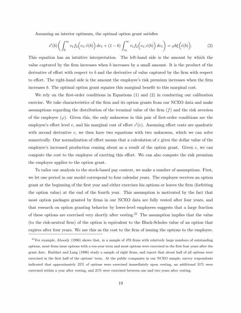
Assuming an interior optimum, the optimal option grant satisfies

e′(b)(∫ v0

0v1f2

(v1; e(b)

)dv1 + (1− b)

∫ ∞v0

v1f2

(v1; e(b)

)dv1

)= ϕbξ

(e(b)

). (2)

This equation has an intuitive interpretation. The left-hand side is the amount by which the

value captured by the firm increases when b increases by a small amount. It is the product of the

derivative of effort with respect to b and the derivative of value captured by the firm with respect

to effort. The right-hand side is the amount the employee’s risk premium increases when the firm

increases b. The optimal option grant equates this marginal benefit to this marginal cost.

We rely on the first-order conditions in Equations (1) and (2) in conducting our calibration

exercise. We take characteristics of the firm and its option grants from our NCEO data and make

assumptions regarding the distribution of the terminal value of the firm (f) and the risk aversion

of the employee (ϕ). Given this, the only unknowns in this pair of first-order conditions are the

employee’s effort level e, and his marginal cost of effort c′(e). Assuming effort costs are quadratic

with second derivative c, we then have two equations with two unknowns, which we can solve

numerically. Our normalization of effort means that a calculation of e gives the dollar value of the

employee’s increased production coming about as a result of the option grant. Given c, we can

compute the cost to the employee of exerting this effort. We can also compute the risk premium

the employee applies to the option grant.

To tailor our analysis to the stock-based pay context, we make a number of assumptions. First,

we let one period in our model correspond to four calendar years. The employee receives an option

grant at the beginning of the first year and either exercises his options or leaves the firm (forfeiting

the option value) at the end of the fourth year. This assumption is motivated by the fact that

most option packages granted by firms in our NCEO data are fully vested after four years, and

that research on option granting behavior by lower-level employees suggests that a large fraction

of these options are exercised very shortly after vesting.21 The assumption implies that the value

(to the risk-neutral firm) of the option is equivalent to the Black-Scholes value of an option that

expires after four years. We use this as the cost to the firm of issuing the options to the employee.

21For example, Aboody (1996) shows that, in a sample of 478 firms with relatively large numbers of outstanding

options, most firms issue options with a ten-year term and most options were exercised in the first four years after the

grant date. Huddart and Lang (1996) study a sample of eight firms, and report that about half of all options were

exercised in the first half of the options’ term. At the public companies in our NCEO sample, survey respondents

indicated that approximately 25% of options were exercised immediately upon vesting, an additional 31% were

exercised within a year after vesting, and 21% were exercised between one and two years after vesting.

19

Second, we assume that the distribution of the terminal value of the firm follows a log-normal

distribution. The mean of this distribution is given by v0(1 + r)4 + e, where v0 is the value of the

firm at time zero, r is the annual expected return on the firm’s shares, and e is the effort level chosen

by the employee. We set r = 10% in our analysis. The standard deviation of this distribution is

given by 2σv0, where σ is the expected annual standard deviation of the firm’s return.

For public companies in our NCEO sample, we estimate a historical value of σ using stock

return data from the Center for Research in Securities Prices (CRSP) from 1995 through 2000. For

the 86 companies that are private or for which historical stock returns are insufficient, we compute

a historical σ using the predicted level from a regression of σ on the firm’s number of employees

using the 130 companies for which we can compute historical volatilities. For our calculation of

option values, we would like to apply expectation of future stock volatility, rather than the historical

volatility we compute. Implied volatilities from options markets show that future and historical

levels are similar in short forward-looking horizons (a year or two), but markets going out four

years do not exist. We therefore assume that future volatilities will be the minimum of 0.75 and

75% as high as the computed historical volatilities.

We consider two possible values for the employee’s level of risk aversion, and two possible

employee cost-of-effort functions. Friend and Blume (1975) and Hall and Murphy (2002) argue

that 2.5 is a rough lower bound on the average person’s coefficient of relative risk aversion (ρ).

To allow for the possibility that option-based pay attracts a selection of risk-tolerant employees,

however, we use a relative risk aversion value of one in our basic specification. We convert this to

an Arrow-Pratt measure of absolute risk aversion (as required by our agency model) by dividing

by the employee’s wealth level, which we assume to be five times the annual salary paid by the

firm to middle managers. We also consider the case where middle managers are of “average” risk

tolerance (that is, ρ = 2.5). In our basic specification, we assume quadratic effort costs with second

derivative c. We also apply c(e) = 14ce

4.

In Table 3, we present a summary of the results from this exercise. We select four firms, one

from each employment size quartile, from our NCEO data. Note first that the value of option

grants to middle managers varies considerably in the sample. The typical firm grants options

with a Black-Scholes value equal to approximately one year of salary, though the “Large Firm” in

column (4) grants three years of salary to new middle managers (worth a total of over a quarter of

a million dollars.) Note, however, that while some of these firms make valuable grants, the middle

manager typically owns a very small fraction of the firm (less than one one-thousandth of a percent

20

Table 3: Calibration — IncentivesSmall Firm Med-Small Firm Med-Large Firm Large Firm Medians

(1) (2) (3) (4) (5)

Employees < 50 < 100 ∼300 10,000+ 180

Middle Manager Salary $38 $100 $90 $90 90

Employee Share (b) 0.015% 0.052% 0.009% 0.00011% 0.0404%

Firm Value (April 2000 – $millions) < $100 ∼$200 ∼ $300 >$50,000 $230

Stock Volatility (σ) > 75% > 75% < 75% >50% 72%

Black-Scholes Value $52 $95 $11 $272 $92

Case One: ρ = 1, c(e) = 12ce2

Effort (e) $10.2 $9.3 $0.18 $63.5 $8.71

Cost of Effort (c(e)) $0.0026 $0.0014 $0.000005 $0.000023 $0.0010

Risk Premium $4.6 $4.3 $0.088 $22.6 $2.76

Case Two: ρ = 2.5, c(e) = 12ce2

Effort (e) $50.6 $35.9 $0.457 $1,511.5 $148.5

Cost of Effort (c(e)) $0.011 $0.0054 $0.000012 $0.0005 $0.011

Risk Premium $11.5 $10.9 $0.22 $56.5 $6.92

Case Three: ρ = 1, c(e) = 14ce4

Effort (e) $31.7 $29.1 $0.683 $223.5 $28.5

Cost of Effort (c(e)) $0.0040 $0.0023 $0.000010 $0.0004 $0.0019

Risk Premium $4.6 $4.3 $0.088 $22.6 $2.76

Risk-free rate is assumed to be 5%. Options assumed to expire in ten years and fully vest in four years. All dollar

values are in thousands except firm value.

21

in the case of the large firm). In contrast, “senior managers” of these same firms get grants of

approximately eight times as many shares and the top executives of some of the bigger firms get

grants that are several orders of magnitude greater than grants to middle managers.22 Therefore,

though the BLS statistics in Section 2 indicate that high paid non-executives, such as the middle

managers we study, receive the majority of total option grants, we expect the incentive effects of

these grants to be very different from those for top executive analyzed by, for example, Hall and

Murphy (2002).

We present results from three calibrations for each of the four firms in the table. The first

calibration assumes quadratic effort costs and absolute risk aversion of one divided by five times

salary. The second assumes quadratic effort costs and absolute risk aversion of 2.5 divided by salary.

The third assumes effort costs of 14ce

4 and absolute risk aversion of one divided by five times salary.

Because one period in our model corresponds to four calendar years, we annualize all figures in our

table by dividing by four. We also display the sample medians for all values in the table.

We focus first on the smallest firm, listed in Column (1). This firm has a small number of

employees, and makes modest option grants to middle-level managers. Assuming quadratic effort

costs and a coefficient of absolute risk aversion of one, our model computes that the employee’s

additional productivity coming about as a result of the option grant is $10,200, annually. The

risk premium the employee attaches to his annual compensation on account of the option grant is

$4,600. The annual cost to the employee of exerting this additional effort is $2.60.

The second calibration for this firm yields larger figures for effort and effort costs. To see the

intuition for this, recall that our model solves for effort using the firm’s first-order condition, which

states that the marginal benefit and marginal cost associated with additional option grants must be

equal. If employees are more risk averse, then the marginal cost to the firm of using option-based

pay is higher. Hence, firms are willing to make the observed grants only if the responsiveness of

effort to incentives is higher. For the small firm, the model indicates that the option grant causes

a middle-level employee to produce an additional $50,600 annually, at annual risk and effort costs

of $11,500 and $11, respectively. The third calibration also yields higher effort figures than did

22The difference between non-executives and top 5 proxy-listed executives (which is the group typically studied) is

very stark in the Execucomp dataset. Using 1996-2002, we used our methodology to estimate the value of grants to

executives and non-executives at firms that meet our “SEC Plan1” criteria. The average (median) grants to the CEO

73 (89) are times as great as grants per non-executive. The average (median) grants to a non-CEO top 5 executive

are 17 (22) times as great as grants per non-executive.

22

the first. The cost-of-effort function here is flatter, meaning employees are more responsive to

low-powered incentives. For the small firm, the model indicates that the option grant causes a

middle-level employee to produce an additional $31,700 annually, at annual risk and effort costs of

$4,600 and $4, respectively.

Calibrations for the three other firms yield widely differing magnitudes. Our medium-large firm

is notable in that it makes small option grants to middle managers. These grants impose small

risk costs on employees, so the model infers that the value created and effort costs incurred by

employees must be small as well. Our largest firm makes grants with a large Black-Scholes value,

but because the firm has a very large number of shares outstanding, the employee’s resulting share

(b) is very small. The model therefore infers that weak incentives must motivate employees to

create a large amount of value. For this firm, the employee creates an additional $63,500 annually,

at risk and effort costs of $22,600 and 2.3 cents.

We conclude from this exercise that the provision of incentives does not appear very plausible

as an explanation for option-based pay. We base this conclusion on the following observation: In

the case of the small firm and the first set of assumptions, options bring $10,200 of additional

benefits into the employee/firm relationship at a total cost (not including the risk costs) of less

than three dollars. If this were the case, it seems clear that the parties’ inability to contract on

effort is generating a very substantial underprovision of effort. This difference, which strikes us as

implausibly large, is implied by our agency model combined with the assumption that observed

option grants reflect optimal incentives. This comparison is even more dramatic in the case of the

large firm, where the additional benefits and costs of options are $63,500 and about two cents,

respectively.

The question we are left with is the following: Couldn’t the firm, at a cost of less than $22,600,

devise some other means of identifying whether an employee has taken actions that increase the

value of the firm at trivial cost to the employee, and then reward the employee directly for these

actions? Or, put another way, if additional effort would bring some amount on the order of $63,500

into the employment relationship at a cost of a few cents, wouldn’t the firm and employee figure

out some way to split that surplus that did not require the employee to bear so much risk that

the surplus was largely depleted? Even if “effort” cannot be objectively measured, it appears to

us relatively straightforward for firms to use various forms of subjective performance evaluation

to reward employees for value they create. Given our calculations here, we find it very difficult

to believe that stock options could be the most efficient incentive mechanism available to firms.

23

The most favorable case that can be made for options-as-incentives is this: options are sensible for

incentive purposes under a very limited set of circumstances — namely, if employees take actions

that have large value implications for the firm, the costs to the employee of taking these actions

are very small, and it is extremely difficult for firms to observe whether employees are taking these

actions.

4.2 Sorting

We now consider the sorting model discussed in Section 3.2, where potential employees vary in their

beliefs about the firm’s prospects. The intuition underlying our sorting calibration is the following:

If sorting drives observed option grants, then the employee must prefer receiving the observed

option package to an all-cash compensation package that costs the firm the same amount. Hence,

we proceed by first computing the cost to the firm (salary plus Black-Scholes value of options) of

observed compensation packages. We assume the firm would be willing to offer the employee an

all-cash package costing the same amount, and then compute the set of values for employee risk

tolerance and beliefs as to the firm’s expected return under which the employee prefers the observed

option package to the all-cash package.

We vary our analysis somewhat from the prior section while retaining most of the same basic

assumptions. Let one period of our model correspond to four calendar years. Suppose again that

options vest after four years, and that the employee exercises all options immediately upon vesting.

Let v1 be the terminal value of the firm, and suppose the employee believes it to be log-normally

distributed with mean v0(1 + r∗)4 and standard deviation 2σv0, where σ is the annual standard

deviation of returns. We determine the options’ value when issued (which we use as the cost to the

firm) using Black-Scholes assuming expiration in four years. Let the employee have constant relative

risk aversion with initial wealth equal to his annual salary.23 We make assumptions regarding tax

rates applied to three types of income: current salary, options profits, and additional cash salary the

employee would receive if he got no stock options. Current salary is inframarginal in this analysis,

so we apply τs = 20% to capture an estimate of average tax rates in calculating utility. The other

two types of earnings are marginal, so we apply τb = 40%.

Results are displayed graphically in Figures 1 through 4. To produce these graphs, we place

the employee’s coefficient of relative risk aversion on the x-axis and his expectation as to the

23While constant absolute risk aversion allowed us to simplify our analysis in the previous section, constant relative

risk aversion is likely more realistic.

24

0%

5%

10%

15%

20%

25%

30%

0.1 0.2 0.3 0.4 0.5 0.6 0.7 0.8 0.9 1.0 1.1 1.2 1.3 1.4 1.5 1.6 1.7 1.8 1.9 2.0 2.1 2.2 2.3 2.4 2.5 2.6 2.7 2.8 2.9 3.0

CRRA Coefficient

Expe

cted

Ann

ual S

tock

Ret

urn

Agent prefers observed cash plus option

package.

Agent would prefer all-cash alternative.

Tax advantage makes option package

preferable.

Figure 1: Small firm employee’s preferences over compensation plans for different values of r∗ and

ρ.

firm’s annual stock return on the y-axis. For each point on this plane, we can compute whether

an employee with these preferences and beliefs prefers the observed option package or an all-cash

package that costs the firm the same amount. We also identify a region in which the tax advantages

tips the employee’s preference toward the option package. The four firms shown in the figures are

the same four that we highlighted in Table 3.

We first consider an employee with coefficient of relative risk aversion 2.5 who expects his

firm’s share price to increase by 10% per year. At our small, medium-small, and large firms

(Figures 1, 2, and 4), such an employee prefers an all-cash package costing the firm the same

amount. The medium-large firm makes small option grants, and such an employee would prefer

the observed salary plus option package because of the tax advantages. These conclusions do not

change markedly when the employee is less risk averse. Lowering the employee’s ρ to 1 does not

justify the use of options at the small, medium-small, or large firm, but the gap between the cost

to the firm and the employee’s valuation becomes smaller.

Next, we keep the employee’s risk aversion relatively low, but assume he expects 25% annual

stock appreciation (four-year appreciation of 144%). The employees at all of the four firms in

25

0%

5%

10%

15%

20%

25%

30%

0.1 0.2 0.3 0.4 0.5 0.6 0.7 0.8 0.9 1.0 1.1 1.2 1.3 1.4 1.5 1.6 1.7 1.8 1.9 2.0 2.1 2.2 2.3 2.4 2.5 2.6 2.7 2.8 2.9 3.0

CRRA Coefficient

Expe

cted

Ann

ual S

tock

Ret

urn


package.



preferable.

Figure 2: Med-Small firm employee’s preferences over compensation plans for different values of r∗

and ρ.

Figures 1 through 4 now prefer the option package, as do the employees at 205 of the 216 firms in

our sample. While 25% may seem like an excessively optimistic expectation, it is well below the

average return at these firms in 1999. If employees naively believe there is momentum in share

prices, then perhaps this figure is not far from accurate.

As discussed in Section 3.2, one reason why firms may attach options to the employment re-

lationship (as opposed to simply letting employees trade on their own accounts) is if optimistic

employees are more productive. If this is the case, then our assertion above that firms are indiffer-

ent between offering observed option packages and an all-cash package costing the firm the same

amount is inaccurate. Firms would strictly prefer the option package if granting it also attracts a

more productive employee. In this case, we can use our estimates from Table 3 to provide an esti-

mate of what level of productivity differences would justify the options grants in the NCEO data.

The expected return in these estimates is 10%, suggesting the employee is only mildly optimistic.

Depending on which firm we consider and what level of risk aversion we assume, optimistic em-

ployees would have to be anywhere from less than $100 to over $50,000 more productive annually.

The required productivity differences at some extreme firms (especially the “large firm” in column

26

0%

5%

10%

15%

20%

25%

30%

0.1 0.2 0.3 0.4 0.5 0.6 0.7 0.8 0.9 1.0 1.1 1.2 1.3 1.4 1.5 1.6 1.7 1.8 1.9 2.0 2.1 2.2 2.3 2.4 2.5 2.6 2.7 2.8 2.9 3.0

CRRA Coefficient

Expe

cted

Ann

ual S

tock

Ret

urn


package.



preferable.

Figure 3: Med-Large firm employee’s preferences over compensation plans for different values of r∗

and ρ.

(4)) seem implausible. However, the differences at the other firms and at the median firm appear

consistent with the possibility that firms are willing to compensate optimistic workers for part of

the risk premium of options compensation in order to attract more productive workers.

In general, we believe these results suggest that the sorting model could be at least a contributing

factor in explaining why some firms offer stock options to lower level employees. If potential

employees are somewhat risk tolerant and have optimistic views about the future of the firm,

then employees will value cash-plus-options packages at more than their cost (net of productivity

differences) to the firm. Full confirmation of this model will require an examination of across-firm

variation in who uses stock options. Our calculations here indicate that, holding the employee’s risk

aversion constant, firms with lower stock volatility can more efficiently use stock options. Firms

in the NCEO sample tend, however, to have very high volatilities. The fact that high-volatility

firms use options is consistent with sorting only if these firms hire a selection of very risk tolerant

employees, if the firm can locate extremely optimistic employees, or if optimistic employees are

significantly more productive.

27

0%

5%

10%

15%

20%

25%

30%

0.1 0.2 0.3 0.4 0.5 0.6 0.7 0.8 0.9 1.0 1.1 1.2 1.3 1.4 1.5 1.6 1.7 1.8 1.9 2.0 2.1 2.2 2.3 2.4 2.5 2.6 2.7 2.8 2.9 3.0

CRRA Coefficient

Expe

cted

Ann

ual S

tock

Ret

urn


package.



preferable.

Figure 4: Large firm employee’s preferences over compensation plans for different values of r∗ and

ρ.

4.3 Retention

We now consider Oyer’s (2003) explanation of option-based pay as a means for indexing the value of

employees’ deferred compensation to their outside options. The intuition underlying our retention

calibration is the following: If options are intended to help firms index wages to market conditions,

then short-run variation in the value of option packages must be of the same order of magnitude as

short-run variation in spot wages. Given our detailed NCEO data on option grants, we can compute

the short-run variation in the value of option packages, and use this to infer firms’ expectations

regarding wage variation.

We adjust the timing of our discussion somewhat to reflect the additional complexity of this

model. Whereas previously we allowed one period in our model to represent four calendar years, we

now assume that one period represents one calendar year. We assume a firm hires an employee at

time t = 0. Between t = 0 and t = 1, one of three states of the world is realized. With probability

qg (qb), industry conditions are revealed to be “good” (“bad”). Conditions are “unchanged” with

probability 1− qg − qb. The firm operates until time t = 4, and then the model ends.

28

Industry conditions affect both labor and financial markets. If industry conditions are good,

then the employee could, at time t = 1 obtain a job offer from another employer that pays wage

Sg. If conditions are unchanged or bad, then the best offer the employee can get is Su or Sb ,

respectively, with Sg > Su > Sb. Share prices are affected as follows:

E[v1 |Good state] = vg

E[v1 |Unchanged state] = vu

E[v1 |Bad state] = vb.

We let the unconditional expectation of v1 equal vu, which implies qh(vg − vu) = qb(vu − vb). We

also assume Var[v1 | s] = (3/5)σ2 for each state s ∈ {g, u, b}. In words, the variance of firm value

conditional on industry prospects is equal to 60% of the unconditional variance, which means 40% of

the total variance is determined by industry conditions.24 To compute the v values, we first assume

an expected rate of return, r, on the firm’s shares. This determines vu, as E[v1] = vu = (1 + r)v0.

We then solve for magnitudes vg and vb so that the unconditional variance of the firm’s return is

equal to σ2.

When making hiring decisions, the firm must decide between offering spot wages and offering

an option-based package. If the firm chooses spot wages, then it pays the employee Su in the first

year. If industry conditions then turn good, the employee seeks an outside offer prior to t = 1. The

firm matches the offer and incurs transaction cost k in doing so.25 If conditions turn bad, then the

firm cannot adjust the employee’s wage downward. After the first-period uncertainty is revealed, no

further changes in industry conditions occur, and the employee works for three additional periods

at the set wage. Hence, the expected cost to the firm of offering the spot wage job is

Su + 3(qgSg + (1− qg)Su

)+ qgk.

An option-based compensation package consists of a salary Sopt and an option grant consisting of

n options with initial Black-Scholes value BS(v0). We assume that the employee decides whether to

24We experimented with other allocations of risk between firms and industries, but found that it made surprisingly

little difference. The choice of 60% idiosyncratic risk is based on several regressions we ran of individual firm returns

on the NASDAQ composite index or the Dow Jones Internet Commerce and Internet Service Indexes. In practice,

the amount of idiosyncratic risk is often reduced by firms’ lowering the strike price of options.

25Alternatively, the parameter k can be interpreted as a turnover cost — if the employee leaves, then the firm hires

a new employee at the prevailing spot wage. Such a cost can arise from training or search.

29

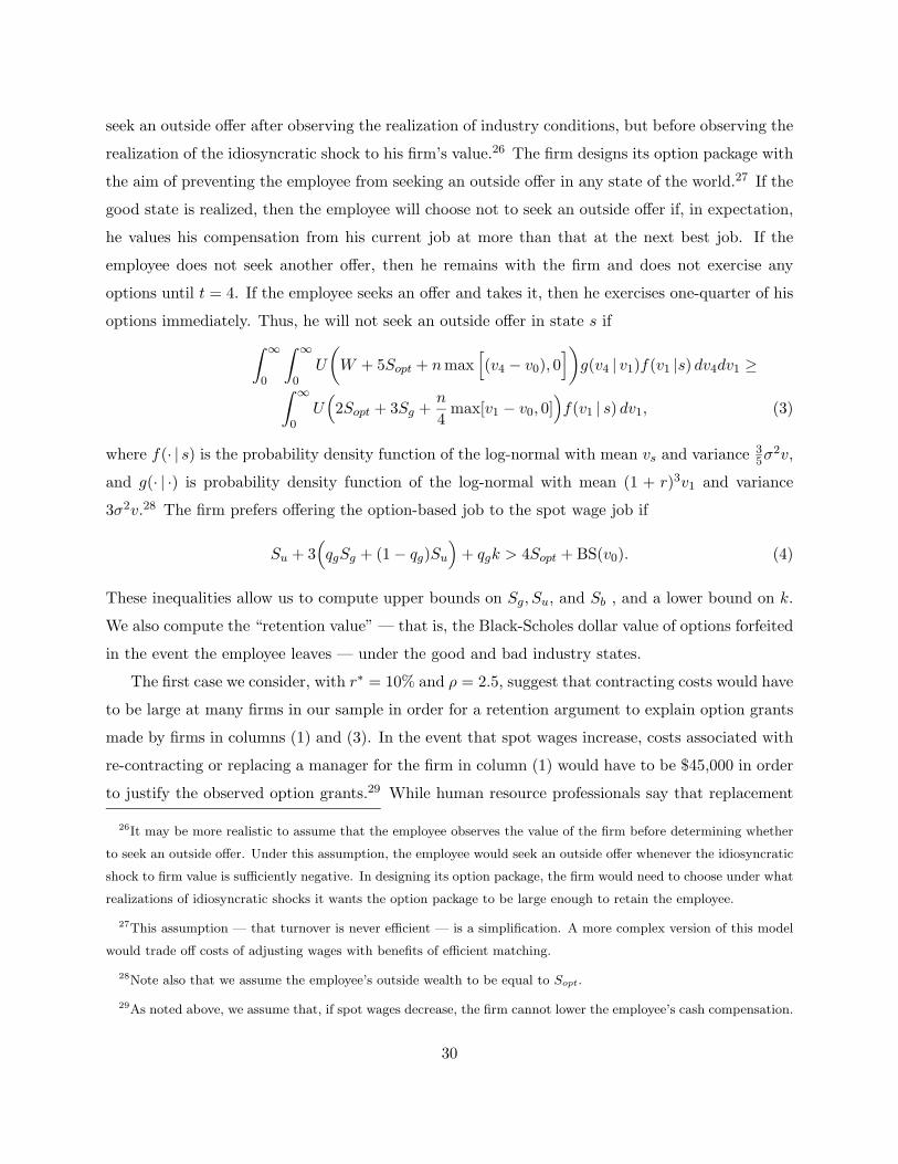
seek an outside offer after observing the realization of industry conditions, but before observing the

realization of the idiosyncratic shock to his firm’s value.26 The firm designs its option package with

the aim of preventing the employee from seeking an outside offer in any state of the world.27 If the

good state is realized, then the employee will choose not to seek an outside offer if, in expectation,

he values his compensation from his current job at more than that at the next best job. If the

employee does not seek another offer, then he remains with the firm and does not exercise any

options until t = 4. If the employee seeks an offer and takes it, then he exercises one-quarter of his

options immediately. Thus, he will not seek an outside offer in state s if∫ ∞0

∫ ∞0

U

(W + 5Sopt + nmax

[(v4 − v0), 0

])g(v4 | v1)f(v1 |s) dv4dv1 ≥∫ ∞

0U(

2Sopt + 3Sg +n

4max[v1 − v0, 0]

)f(v1 | s) dv1, (3)

where f(· | s) is the probability density function of the log-normal with mean vs and variance 35σ

2v,

and g(· | ·) is probability density function of the log-normal with mean (1 + r)3v1 and variance

3σ2v.28 The firm prefers offering the option-based job to the spot wage job if

Su + 3(qgSg + (1− qg)Su

)+ qgk > 4Sopt + BS(v0). (4)

These inequalities allow us to compute upper bounds on Sg, Su, and Sb , and a lower bound on k.

We also compute the “retention value” — that is, the Black-Scholes dollar value of options forfeited

in the event the employee leaves — under the good and bad industry states.

The first case we consider, with r∗ = 10% and ρ = 2.5, suggest that contracting costs would have

to be large at many firms in our sample in order for a retention argument to explain option grants

made by firms in columns (1) and (3). In the event that spot wages increase, costs associated with

re-contracting or replacing a manager for the firm in column (1) would have to be $45,000 in order

to justify the observed option grants.29 While human resource professionals say that replacement

26It may be more realistic to assume that the employee observes the value of the firm before determining whether

to seek an outside offer. Under this assumption, the employee would seek an outside offer whenever the idiosyncratic

shock to firm value is sufficiently negative. In designing its option package, the firm would need to choose under what

realizations of idiosyncratic shocks it wants the option package to be large enough to retain the employee.

27This assumption — that turnover is never efficient — is a simplification. A more complex version of this model

would trade off costs of adjusting wages with benefits of efficient matching.

28Note also that we assume the employee’s outside wealth to be equal to Sopt.

29As noted above, we assume that, if spot wages decrease, the firm cannot lower the employee’s cash compensation.

30

Table 4: Calibration — RetentionSmall Firm Med-Small Firm Med-Large Firm Large Firm Median

(1) (2) (3) (4) (5)

Annual Cash Compensation (from NCEO survey)

$38 $100 $90 $90 $90

Case One: r∗ = 10%, ρ = 2.5

Initial Spot Wage (Su) $41.3 $109.1 $92.3 $126.4 $92.6

High Spot Wage (Sg) $42.7 $112.6 $93.5 $139.5 $93.7

Low Spot Wage (Sb) $39.1 $104.1 $90.9 $113.3 $90.5

Retention Value – High $44.8 $71.6 $9.7 $190.8 $71.0

Retention Value – Low $6.7 $10.7 $1.5 $60.1 $15.6

Transaction Cost (k) $45.3 $10.9 $0 $14.0 $33.3

Case Two: r∗ = 10%, ρ = 1

Initial Spot Wage (Su) $44.6 $113.9 $92.6 $144.6 $99.4

High Spot Wage (Sg) $48.3 $121.2 $94.1 $166.5 $104.6

Low Spot Wage (Sb) $40.1 $105.6 $91.0 $123.6 $91.6



Transaction Cost (k) $0 $0 $0 $0 $0

Case Three: r∗ = 25%, ρ = 1

Initial Spot Wage (Su) $51.5 $126 7 $95.2 $241.7 $113.1

High Spot Wage (Sg) $57.8 $138.7 $97.7 $284.7 $125.3

Low Spot Wage (Sb) $44.4 $113.4 $92.5 $199.1 $100.6



Transaction Cost (k) $0 $0 $0 $0 $0

Risk-free rate is assumed to be 5%. “Initial spot wage” is the implied market wage when middle manager receives

the options grant and, if there is no common shock, one year later. “High spot wage” (“Low spot wage”) is the

implied maximum market wage for a middle manager one year after the options are granted and after a positive

(negative) common shock. “Transaction cost” is the minimum expected costs the firm would incur over a four year

period due to changes in the agent’s compensation package and/or replacing the agent in order to justify the

amount of stock options it grants to a middle manager. “Retention value” indicates expected Black-Scholes value

(assuming he expects to exercise options four years after they are issued) forfeited if the employee takes the outside

offer, given the value of the common shock.

31

costs can be 25 to 50% of annual wages for some jobs, our estimates for the small firm and the

median firm are at the high end of this range.

The second case, which assumes the worker is risk averse but less so (ρ = 1), lead to much more

plausible estimates of the turnover or renegotiation costs necessary to justify the use of options.

In all four firms in the table, for the median firm, and for a total of 134 of the 216 firms in our

sample, our estimates suggest that firms benefit from using options even if they do not lower the

cost of raising an employee’s wage. That is, the firms in the table can justify the use of options

at any positive turnover cost.30 However, for this conclusion to be credible, the model suggests

that options can be used for retention purposes if spot wages fluctuate up or down anywhere from

$2,000 to $20,000 over a short period. In this second set of estimates, the turnover or renegotiation

costs are negligible and the amount of unvested option value would have a significant effect on

employee retention. Therefore, the results suggest that the retention model can justify the use

of stock options, if market wages for managers in this sample really vary by as much as Table 4

suggests.

The third case combines the sorting and retention models, by assuming the employee is opti-

mistic regarding the firm’s share price. Here, the retention argument can explain option grants even

if spot wages vary $5,000 to $40,000 over a short horizon. The retention values grow as employees

value their holdings more highly, and the critical values of turnover costs fall even further below

zero. Note that the assumptions underlying the retention model reinforce the sorting model be-

cause, by assuming stock options only expose the employee to idiosyncratic risk on the margin, they

lower the risk premium the employee would otherwise need to be paid. We therefore believe that

the last two subsections and the bottom part of Table 4 provide evidence that some combination

of sorting and retention could be contributing to decisions to issue stock options firm-wide.

As a result, our estimates of renegotiation costs only relate to the case of retaining the worker if his spot market wage

increases.

30All else equal, options are relatively more attractive to employees in this section’s analysis than in section 4.2

because employees are exposed to some risk regardless of what form their compensation takes. If the firm offers the

spot wage job, the employee’s compensation will fluctuate due to changes in spot wages.

32

5 Cross-Firm Variation in Option Plans

In this section, we analyze cross-sectional variation in option plan adoption using our SEC data.31

We estimate a series of logit models using “SEC Plan,” as defined in Section 2, as our dependent

variable. To verify that our findings are not sensitive to the definition of our dependent variable,

we define two additional indicators of option plans. SEC Plan2 equals one if the Black-Scholes

value of options granted per non-executive employee in 1998 was at least $1,000. Option grants

are disproportionately made to new employees, so we construct a third indicator — SEC Plan3

— that adjusts for the possibility that option granting behavior depends on employment growth.

We assume that all non-executive grants are given to new employees, and estimate the number of

new employees to be the sum of the 1997 to 1998 increase in employment and 10% of the 1997

employment. We then set SEC Plan3 equal to one if the Black-Scholes value of options granted to

each new employee is at least $2,500. Because these additional variables are constructed using the

market value of options granted, they are, by definition, related to firm and/or industry volatility.

In regressions using these variables, we omit firm and industry volatility.

The explanatory variables include measures related to the comparative static implications of

each model, as well as control variables. All of our analyses include controls for the log of the

number of employees at the firm, the growth in number of employees from 1997 to 1998, and

an indicator variable for “new economy” status, as defined above. Note the predicted effects of

these controls on option usage do not vary in a way that would allow us to distinguish between

the models. In unreported specifications, we also controlled for two-digit SIC code. This did not

materially affect the results.

Agency theory predicts a negative relationship between risk and incentives, so the incentive

model implies that option plans should be less common at high volatility firms. If higher volatility

also reflects higher variance in people’s beliefs about a firm, then the sorting model predicts that

higher volatility firms (or firms in higher volatility industries) will be more likely to make broad

option grants. The retention model predicts that non-executive option plans will be negatively

related to idiosyncratic firm volatility, but positively related to the volatility of the set of firms that

compete for a given group of employees. To test these implications, we use two volatility measures

as explanatory variables. First, we include monthly firm stock volatility. In addition, we include

31We use the SEC data because it constitutes a random sample of public firms. However, we redid the analysis in

this section for each year from 1996 through 2001 using all firms in Standard & Poors Execucomp dataset. Virtually

without exception, that analysis led to the same conclusions as the results we present below.

33

“industry volatility,” which we define as the standard deviation of the monthly average return for

all CRSP firms in a given 4-digit SIC code industry.32

The retention model predicts that option plans will be more common at firms whose returns

are more closely related to the returns of other firms that compete for the same set of workers. To

test this implication, we generated a variable that we refer to as “industry volatility share.” To

construct this variable, we first run regressions of each CRSP firm’s monthly returns on industry

returns.33 We average the R2 from these regressions and define this as the industry volatility share.

Finally, we include variables that proxy for variance in potential employees’ beliefs about future

returns and financing constraints. These include an indicator variable for positive cash flow in

1998, 1998 cash flow as a fraction of beginning-of-year capital, and 1998 investment as a fraction

of beginning-of-year capital. We also include cash flow and investment as a fraction of beginning-

of-year market capitalization.

Results are in Table 5. First, note that option plans are more common at smaller firms and new

economy firms. Firms with more employees are significantly less likely to have broad stock option

plans. A firm with 10% more employees than another firm is one to one-and-a-half percentage

points less likely to have a broad-based plan.34 New economy firms have a 33 percentage point

higher probability of using a broad-based plan, holding the other factors in column (1) constant.

In contrast to the basic agency theory of an inverse risk/incentive relationship, we find that

a firm with volatility that is 10 percentage points higher than another firm is more likely by 13

percentage points (that is, the probability increases by about one third) to have a broad plan. This

provides further support for our conclusion in Section 4.1 that incentives are not an important

cause of firms’ decision to adopt broad option plans. The dramatically higher volatility of plan

firms (and, as discussed below, their industries) contradicts every “informativeness” agency model.

Column (2) shows that the positive relationship between risk and option plans is largely driven

by industry volatility rather than idiosyncratic firm volatility. Industry volatility is positively (and

32We exclude observations where there are not at least eight firms available to construct industry return.

33For inclusion here, we require firms to have twelve observations of monthly returns.

34Core and Guay (2001) report the opposite result, namely that the value of options grants per employee increases

with firm size. Recall from our discussion in Section 2 that they define any option grant to an employee other than

the five highest paid executives as a grant to a “non-executive.” When we apply their definition, we also find that the

likelihood of broad option plans increases with firm size. Thus, it seems their finding may be indicative that non-top

five executives receive larger option grants at larger firms. Also note that this negative size/option plan relationship

holds up in every year of the Execucomp dataset.

34

significantly) related to option plans and, when controlling for industry volatility, firm volatility is

not significantly related to option plans. This is consistent with the industry versus firm volatility

prediction of the retention model.35 While the sorting model does not have as explicit a prediction

about the relative importance of industry and firm volatility, this model is also consistent with the

results in Table 5 if volatility is correlated with variance in employees’ expectations about future

returns.

We also add “industry volatility share” as an explanatory variable in column (2) and in the

logits that use SEC Plan2 and SEC Plan3 as the dependent variable. While this variable does not

show a significant relationship to option plan status in columns (2) and (6), it is positively and

significantly related to SEC Plan2. This is consistent with the retention model because it suggests

that firms are more likely to grant options if their returns are more closely related to other firms

that could employ their workers.

In column (2), we find that positive cash flow is associated with a 22 percentage point lower

probability (that is, it drops by approximately two thirds) of implementing a broad-based stock

option plan. While this provides some potential support for the financing constraints hypothesis,

columns (4) show that the other controls for financing constraints are not related to option grants.

When we use SEC Plan2 or SEC Plan3 as the dependent variable, we find that firms that are

making large investments relative to capital are more likely to have option plans. However, firms

that are making larger investments relative to the value of their equity are, if anything, less likely

to have option plans.

We believe the relationship between cash flow and option plans (and between investments and

option plans) is consistent with the sorting model. Making investments (either in capital or in

funding negative cash flow operations) does not necessarily indicate that a firm faces financing

constraints. On the other hand, it does seem that investing firms are likely to be firms where

future returns are variable and where the expectations about future returns vary across potential

employees. If this is true, this suggests that firms are financing through employees when there are

employees whose beliefs make them a relatively inexpensive source of capital.

We believe that the results in Table 5 are consistent with both the sorting and retention models,

but they provide little reason to reverse our belief that incentive effects are not important in broad-

based option plans. Though the negative association between employees and option plans would

35Carter and Lynch (2003) provide related cross-sectional support for the importance of retention. They show that

option repricing is correlated with reductions in employee turnover.

35

Table 5: SEC Option Plan LogitsDependent Variable SEC Plan SEC Plan SEC Plan SEC Plan SEC Plan2 SEC Plan3

(1) (2) (3) (4) (5) (6)

Log Employees -0.1472 -0.1188 -0.1209 -0.1231 -0.1770 -0.1226

(0.0146) (0.0172) (0.0196) (0.0181) (0.0228) (0.0190)

Employee Growth 0.0763 0.0817 0.0310 0.0562 0.0702 -0.0449

(0.0441) (0.0485) (0.0383) (0.0478) (0.0545) (0.0163)

Firm Volatility 1.3232 0.6306 0.3029 0.5436

(0.3279) (0.4071) (0.4212) (0.4183)

New Economy 0.3291 0.2764 0.2512 0.2815 0.3512 0.1912

(0.0676) (0.0738) (0.0757) (0.0749) (0.0775) (0.0666)

Positive Cash Flow -0.2215 -0.2256 -0.2225 -0.2371 0.0574

(0.0745) (0.0749) (0.0827) (0.0779) (0.0710)

Industry Volatility 2.3205 1.9704 2.1861

(0.9440) (0.9881) (0.9497)

Industry Volatility Share -0.0831 0.5065 0.1888

(0.1780) (0.2106) (0.1878)

Investment/Value -0.1125 -0.6078 -0.3424

(0.1919) (0.2741) (0.2227)

Investment/Capital 0.1123 0.1832 0.3473

(0.0602) (0.0719) (0.0776)

Cash Flow/Value -0.0504

(0.1475)

Cash Flow/Capital 0.0016

(0.0040)

Pseudo-R2 0.2818 0.2763 0.3057 0.2822 0.3962 0.2234

Sample Size 765 573 479 549 479 439

Dependent variables, described in the text, are various indicator variables for whether a firm has a

broad-based stock option plan. Data are from a random sample of 1,000 firms that filed annual reports and

proxy statements with the SEC in 1999. Sample size in each logit is based on the number of firms for

which financial information, as well as industry stock return, was available. “New Economy” indicates

primary SIC code is 3570-3579, 3661, 3674, 5045, 5961, or 7370-7379. Coefficients are marginal effects on

the probability that the firm has a plan. Standard errors are in parentheses.

36

lend some support to the moral hazard explanation of option use, our previous numerical analysis

suggests that the marginal effects of the number of employees on incentives dissipate quickly as

a firm grows and that these firms are generally above the level where we would expect such an

association between size and incentives. More importantly, the strong positive relationship between

risk and option plans contradicts a central prediction of the incentive model.

6 Conclusion

Using firm-level data on stock option grants and financial information, we have tried to reconcile the

fact that some firms issue stock options to lower-level employees with economic theory. We focused

on three classes of model – moral hazard, sorting on worker beliefs about the firm’s prospects, and

stock options as a relatively inexpensive way to adjust worker compensation to market conditions.

Using details on the stock option plans for middle managers at a sample of over 200 firms, we

showed that stock options appear to be an incredibly inefficient means of providing incentives to

employees. By calibrating an agency model to data on actual grants of stock options to middle-level

employees, we computed that risk premia associated with these grants are typically several orders

of magnitude larger than the cost to employees of the resulting increases in effort. Our calibrations

suggest that, if a typical firm in our sample were granting options to middle managers as a means of

inducing them to increase effort, the firm would be paying each employee many thousands of dollars

in risk premium in order to generate added effort that the employee values at less (often much less)

than $100. We conclude, based on these calculations, that stock options are an inefficient incentive

mechanism for middle managers.

Though we cannot conclusively determine how important either model is, we interpret our

analysis as consistent with both the sorting and retention models. We show that, if workers are

sufficiently optimistic about their employers’ prospects, stock options may be an efficient means

of compensation. That is, despite demanding compensation for risk, optimistic employees may

be willing to accept a large enough reduction in cash compensation to warrant using options as

compensation. We also show that, if spot labor market rates are fairly variable and reducing worker

wages is costly, then the correlation between the value of a worker’s stock option holdings and his

reservation utility may induce the firm to issue stock options.

We believe that neither accounting treatment of option grants, cash constraints, nor any of the

three models we examined in this paper can single-handedly explain the use of broad-based stock

37

option plans. The belief that the accounting treatment of options is solely responsible for their

widespread use seems inconsistent with the cross-sectional variation in adoption of option plans

and with the fact that so many firms with broad plans have been successful for long periods. As

we discussed in Section 3.4, employees are too expensive a source of capital to justify the cash

constraints explanation. We believe our estimates in Section 4.1 rule out the incentive model as a

primary (much less exclusive) justification for broad option plans.

We think that the evidence in this paper suggests that sorting or retention may be first-order

determinants of a typical firm’s decision to adopt a broad-based stock option plan. But neither

explanation can stand completely on its own. The sorting model begs a critical question of why firms

and employees would agree to make employees’ beliefs part of an inflexible employment contract,

given that the tax advantages of using options are not very large relative to cash compensation. We

also believe that, while we have demonstrated that stock options can be a useful tool for making

compensation vary with an employee’s market wage, it is a fairly crude tool for this purpose. If firms

received no other benefits from option grants besides savings on the costs of adjusting compensation

agreements, it seems likely they would try to find more specialized measures of employee’s market

value that did not expose the employee to so much idiosyncratic firm risk. It is therefore our

belief that the firms that adopt broad option plans are those where the returns to cost effectively

attracting and retaining employees is particularly high. But those firms may well choose option

plans (as opposed to stock grants, profit sharing, or other pay mechanisms) as a means towards

these ends for secondary reasons such as accounting treatment or a need to find a simple metric

upon which to base pay.

38

References

Aboody, D.: 1996, Market valuation of employee stock options, Journal of Accounting and Economics

22, 357–391.

Aboody, D., Barth, M. E. and Kasznik, R.: 2001, SFAS 123 stock-based compensation expense and equity

market values, Research Paper 1694, Graduate School of Business, Stanford University.

Aggarwal, R. and Samwick, A. A.: 1999, The other side of the tradeoff: The impact of risk on executive

compensation, Journal of Political Economy 108, 65–105.

Barron, J. M. and Waddell, G. R.: 2003a, Executive rank, pay and project selection, Journal of Financial

Economics 67, 305–349.

Barron, J. M. and Waddell, G. R.: 2003b, Hard work versus good intentions: Stock options as compensation.

Purdue University and University of Oregon.

Bell, T., Landsman, W., Miller, B. and Yeh, S.: 2002, The valuation implications of employee stock-option

accounting for profitable computer software firms, Accounting Review 77, 971–996.

Bergman, N. and Jenter, D.: 2003, A note on employee sentiment and stock option compensation. Sloan

School, Massachusetts Institute of Technology.

Bull, C.: 1987, The existence of self-enforcing implicit contracts, Quarterly Journal of Economics 102, 147–

160.

Bushman, R. M., Indjejikian, R. J. and Smith, A.: 1995, Aggregate performance measures in business

unit manager compensation: The role of intrafirm interdependencies, Journal of Accounting Research

33, 101–128.

Carter, M. E. and Lynch, L. J.: 2003, The effect of stock option repricing on employee turnover. The

Wharton School, University of Pennsylvania and Darden Graduate School of Business, University of

Virginia.

Core, J. E. and Guay, W. R.: 2001, Stock option plans for non-executive employees, Journal of Financial

Economics 60, 253–267.

Friend, I. and Blume, M. R.: 1975, The demand for risky assets, American Economic Review 65, 900–922.

Garvey, G. T. and Milbourn, T. T.: 2002, Do stock prices incorporate the potential dilution of employee

stock options? Claremont Graduate School and Washington University.

Gompers, P. A., Ishii, J. L. and Metrick, A.: 2003, Corporate governance and equity prices, Quarterly

Journal of Economics 118, 107–155.

Hall, B. J. and Murphy, K. J.: 2002, Stock options for undiversified executives, Journal of Accounting and

Economics 33. 3-42.

39

Hall, B. J. and Murphy, K. J.: 2003, The trouble with stock options, Journal of Economic Perspectives 17.

Forthcoming.

Holmstrom, B. and Milgrom, P. R.: 1987, Aggregation and linearity in the provision of intertemporal

incentives, Econometrica 55, 308–328.

Holmstrom, B. and Milgrom, P. R.: 1991, Multi-task principal-agent analyses: Incentive contracts, asset

ownership and job design, Journal of Law, Economics and Organization 7, 524–552.

Huddart, S. and Lang, M.: 1996, Employee stock option exercises: An empirical analysis, Journal of Ac-

counting and Economics 21, 5–43.

Huddart, S. and Lang, M.: 2003, Information distribution within firms: Evidence from stock option exercises,

Journal of Accounting and Economics 34, 3–31.

Huson, M. R., Scott, T. W. and Wier, H. A.: 2001, Earnings dilution and the explanatory power of earnings

for returns, Accounting Review 76, 589–612.

Ittner, C. D., Lambert, R. A. and Larcker, D. F.: 2003, The structure and performance of equity grants to

employees of new economy firms, Journal of Accounting and Economics 34, 89–127.

Jin, L.: 2002, CEO compensation, diversification, and incentives, Journal of Financial Economics 66, 29–63.

Keating, A. S.: 1997, Determinants of divisional performance evaluation practices, Journal of Accounting

and Economics 24, 243–273.

Kedia, S. and Mozumdar, A.: 2002, Performance impact of employee stock options. Working Paper, Harvard

Business School.

Kruse, D. L.: 1993, Profit Sharing: Does it Make a Difference?, W.E. Upjohn Institute for Employment

Research, Kalamazoo, MI.

Lazear, E. P.: 2001, Output-based pay: Incentives, retention or sorting? Stanford University.

McDonald, R. L.: 2003, The tax (dis)advantage of a firm issuing options on its own stock, Journal of Public

Economics . Forthcoming.

Mehran, H. and Tracy, J.: 2001, The effect of employee stock options on the evolution of compensation in

the 1990s, Federal Reserve Bank of New York Economic Policy Review 7, 17–34.

Murphy, K. J.: 2000, Executive compensation, in O. Ashenfelter and D. Card (eds), Handbook of Labor

Economics, Vol. 3, North-Holland, Amsterdam.

Oyer, P.: 2003, Why do firms use incentives that have no incentive effects?, Journal of Finance . Forthcoming.

Oyer, P. and Schaefer, S.: 2003, A comparison of options, restricted stock, and cash for employee compen-

sation. Stanford Graduate School of Business.

40

Prendergast, C.: 2002, The tenuous trade-off between risk and incentives, Journal of Political Economy

110, 1071–1102.

Sesil, J. C., Kroumova, M. K., Blasi, J. R. and Kruse, D. L.: 2002, Broad-based employee stock options in

U.S. ‘new economy’ firms, British Journal of Industrial Relations 40, 273–294.

Stein, J. C.: 2001, Agency, information, and corporate investment, in G. Constantinides, M. Harris and

R. Stulz (eds), Handbook of the Economics of Finance, Vol. 1, North-Holland.

Weitzman, M. L. and Kruse, D. L.: 1990, Profit sharing and productivity, in A. S. Blinder (ed.), Paying for

Productivity, The Brookings Institution.

41

NBER WORKING PAPER SERIES WHY DO … WORKING PAPER SERIES WHY DO SOME FIRMS GIVE STOCK OPTIONS TO...

Documents

Transcript of NBER WORKING PAPER SERIES WHY DO … WORKING PAPER SERIES WHY DO SOME FIRMS GIVE STOCK OPTIONS TO...