NBER WORKING PAPER SERIES

THE MARKET PRICE OF CREDIT RISK:

AN EMPIRICAL ANALYSIS OF INTEREST RATE SWAP SPREADS

Jun Liu

Francis A. Longstaff

Ravit E. Mandell

Working Paper 8990

http://www.nber.org/papers/w8990

NATIONAL BUREAU OF ECONOMIC RESEARCH

1050 Massachusetts Avenue

Cambridge, MA 02138

June 2002

We are grateful for the many helpful comments and contributions of Don Chin, Qiang Dai, Robert Goldstein,

Gary Gorton, Peter Hirsch, Antti Ilmanen, Deborah Lucas, Josh Mandell, Yoshihiro Mikami, Jun Pan,

Monica Piazzesi, Walter Robinson, Pedro Santa-Clara, Janet Showers, Ken Singleton, Suresh Sundaresan,

Abraham Thomas, Rossen Valkanov, Toshiki Yotsuzuka, and seminar participants at Barclays Global

Investors, Citigroup, Greenwich Capital Markets, Invesco, Mizuho Financial Group, Simplex Asset

Management, UCLA, the 2001 Western Finance Association meetings, the 2002 American Finance

Association meetings, and the Risk Conferences on Credit Risk in London and New York. We are

particularly grateful for the comments and suggestions of the editor William Schwert and an anonymous

referee. All errors are our responsibility. The views expressed herein are those of the authors and not

necessarily those of the National Bureau of Economic Research.

© 2002 by Jun Liu, Francis A. Longstaff and Ravit E. Mandell. All rights reserved. Short sections of text,

not to exceed two paragraphs, may be quoted without explicit permission provided that full credit, including

© notice, is given to the source.

The Market Price of Credit Risk: An Empirical Analysis of Interest Rate Swap Spreads

Jun Liu, Francis A. Longstaff and Ravit E. Mandell

NBER Working Paper No. 8990

June 2002

JEL No. E4

ABSTRACT

This paper studies the market price of credit risk incorporated into one of the most important

credit spreads in the financial markets: interest rate swap spreads. Our approach consists of jointly

modeling the swap and Treasury term structures using a general five-factor affine credit framework and

estimating the parameters by maximum likelihood. We solve for the implied special financing rate for

Treasury bonds and find that the liquidity component of on-the-run bond prices can be significant. We

also find that credit premia in swap spreads are positive on average. These premia, however, vary

significantly over time and were actually negative for much of the 1990s.

Jun Liu Francis A. Longstaff Ravit E. Mandell

UCLA UCLA Salomon Smith Barney

Anderson School Anderson School

110 Westwood Plaza, Box 951481

Los Angeles, CA 90095-1481

and NBER

francis.longstaff@anderson.ucla.edu

1. INTRODUCTION

One of the most fundamental issues in finance is how the market compensates investorsfor bearing credit risk. Events such the flight to quality that led to the hedge fundcrisis of 1998 demonstrate that changes in the willingness to bear credit risk can havedramatic effects on the financial markets. Furthermore, these events indicate thatvariation in credit spreads may reflect both changes in perceived default risk and inthe relative liquidity of bonds. Understanding the risk and return tradeoffs for thesetypes of securities may become even more important in the future if the supply of U.S.Treasury securities available in the market decreases.

This paper studies the market price of credit risk incorporated into what is rapidlybecoming one of the most important credit spreads in the financial markets: interestrate swap spreads. Since swap spreads represent the difference between swap ratesand Treasury bond yields, they reflect the difference in the default risk of the financialsector quoting Libor rates and the U.S. Treasury. In addition, swap spreads mayinclude a significant liquidity component if the relevant Treasury bond trades specialin the repo market. Thus, swap spreads represent an important data set for examininghow both default and liquidity risks influence security returns. The importance of swapspreads derives from the dramatic recent growth in the notional amount of interestrate swaps outstanding relative to the size of the Treasury bond market. For example,the total amount of Treasury debt outstanding at the end of June 2001 was $5.7trillion. In contrast, the Bank for International Settlements (BIS) estimates that thetotal notional amount of interest rate swaps outstanding at the end of June 2001 was$57.2 trillion, representing ten times the amount of Treasury debt.

Since swap spreads are fundamentally credit spreads, our approach consists ofjointly modeling the interest rate swap and Treasury term structures using the reduced-form credit framework of Duffie and Singleton (1997, 1999). To capture the rich dy-namics of the swap and Treasury curves, we use a five-factor affine term structuremodel which allows the swap spread to be correlated with the riskless rate. In ad-dition, our specification allows market prices of risk to vary over time to reflect thepossibility that the willingness of investors to bear credit and liquidity risk may change.We estimate the parameters of the model by maximum likelihood. The data for thestudy spans nearly the full history of the swap market. We show that both the swapand Treasury term structures are well described by the five-factor affine model.

A number of interesting results emerge from this analysis. First, we solve for theshort-term riskless rate implied by Treasury bond prices. We find that the impliedriskless rate can differ substantially from the Treasury-bill rate and is often muchhigher. This is consistent with the widespread view on Wall Street that because of

1

the extreme liquidity of Treasury bills, their yields tend to underestimate the effectiveriskless rate. Since the implied short-term riskless rate could also be interpreted asspecial repo rate for the on-the-run Treasury bonds in the sample, we contrast themwith repo rates for generic or general Treasury collateral.1 We find that these impliedspecial repo rates are slightly less than the general repo rates on average, suggestingthat the prices of the on-the-run Treasury bonds in the sample include premia for theirliquidity or specialness relative to off-the-run Treasury securities. These specialnesspremia can be large in economic terms. For example, the specialness premium for theten-year Treasury note can be as much as 0.57 percent of its notional amount. Theestimated specialness premia match closely those implied by a sample of market termspecial repo rates provided to us.

We then solve for the implied spread process. We find that this spread variessignificantly over time, but is nearly zero for an extended period during the mid tolatter 1990s. Interestingly, much of the variation in the implied credit spread is relatedto the difference between the general and implied special repo rates, suggesting thatchanges in the liquidity of Treasury bonds may be one of the major driving factors ofswap spreads.

Finally, we examine the implications of the model for the market prices of interest-rate and credit-related risk. Consistent with previous research, we find that there aresignificant time-varying term premia embedded in Treasury bond prices. We also findthat there are significant credit premia embedded in the swap curve. On average,these premia are positive, ranging from 0.1 basis points for a one-year horizon to 45basis points for a ten-year horizon. These credit premia also display substantial timevariation. Surprisingly, we find evidence that credit premia were often negative duringan extended period in the 1990s. These results suggest that there have been majorchanges over time in the expected returns from bearing the default and liquidity riskinherent in interest rate swaps.

This paper complements and extends the recent paper by Duffie and Singleton(1997) who apply a reduced-form credit modeling approach to the swap curve andexamine the properties of swap spreads. Our results support their finding that bothdefault-risk and liquidity components are present in swap spreads. By modeling boththe swap and Treasury curves simultaneously, however, we are also able to addressthe issue of how credit risk is priced in the market, which is the primary focus ofthis paper. Another related paper is He (2000) who independently uses a multi-factoraffine term structure framework similar to ours in modeling swap spreads. While Hedoes not estimate the parameters of his model, our empirical results provide supportfor both swap spread modeling frameworks. Grinblatt (2001) models the swap spread

1In a recent paper, Duffie (1996) studies the causes and effects of special repo ratesin the Treasury repo market. See also Sundaresan (1994), Jordan and Jordan (1997),Buraschi and Menini (2001), and Krishnamurthy (2001).

2

as the annuitized value of an instantaneous convenience yield. If this convenience yieldis interpreted as the liquidity component of the spread process, then our results canalso be viewed as providing support for the implications of his model. Other relatedpapers include Sun, Sundaresan, and Wang (1993) who study the extent to whichcounterparty credit risk affects market swap rates, and Collin-Dufresne and Solnik(2001) who focus on the spread between Libor corporate rates and swap rates.

The remainder of this paper is organized as follows. Section 2 explains the frame-work used to model the swap and Treasury term structures. Section 3 describes thedata. Section 4 discusses the maximum likelihood estimation of the model. Section5 focuses on the implications of the results for the liquidity of Treasury securities.Section 6 discusses the empirical results about the properties of swap spreads. Sec-tion 7 presents the results about the pricing of default and liquidity risk. Section 8summarizes the results and makes concluding remarks.

2. MODELING SWAP SPREADS

To understand how the market prices credit risk over time, we need a framework forestimating expected returns implied by the swap and Treasury term structures. Inthis section, we use the Duffie and Singleton (1997, 1999) credit modeling approachas the underlying framework in which to analyze the behavior of swap spreads. Inparticular, we jointly model the swap and Treasury term structures using a five-factoraffine framework and estimate the parameters of the model by maximum likelihood.2

Recall that under standard no-arbitrage assumptions, the value D(t, T ) of a risk-less zero-coupon bond with maturity date T can be expressed as

D(t, T ) = EQ exp −T

t

rs ds , (1)

where r denotes the instantaneous riskless rate and the expectation is taken withrespect to the risk-neutral measure Q rather than the objective measure P . In theDuffie and Singleton (1997, 1999) framework, default is modeled as the realization of aPoisson process with an intensity which may be time varying. Under some assumptionsabout the nature of recovery in the event of default, they demonstrate that the valueof a risky zero-coupon bond C(t, T ) can be expressed in the following form

2Other examples of affine credit models include Duffee (1999, 2002), He (2000), Duffie,Pedersen, and Singleton (2000), Duffie and Liu (2001), and Colin-Dufresne and Solnik(2001).

3

C(t, T ) = EQ exp −T

t

rs + λs ds , (2)

where λ is a credit-spread process.3 They also show that this credit-spread process maybe viewed as the product of the time-varying Poisson intensity and the recovery-rateprocess. Furthermore, they argue that the credit-spread process could also include atime-varying liquidity component which may be either positive or negative. In thispaper, we simply refer to λ as the credit-spread process, keeping in mind, however,that λmay include both default-risk and liquidity components. Consequently, the termcredit risk is used in a general sense throughout this paper, reflecting that variationin credit or swap spreads may be due to changes in either default risk or liquidity.

In applying this credit model to swaps, we are implicitly making two assump-tions. First, we assume that there is no counterparty credit risk. This is consistentwith recent papers by Grinblatt (2001), Duffie and Singleton (1997), and He (2000)that argue that the effects of counterparty credit risk on market swap rates shouldbe negligible because of the standard marking-to-market or posting-of-collateral andhaircut requirements almost universally applied in swap markets.4 Second, we makethe relatively weak assumption that the credit risk inherent in the Libor rate (whichdetermines the swap rate) can be modeled as the credit risk of a single defaultableentity. In actuality, the Libor rate is a composite of rates quoted by 16 banks and,as such, need not represent the credit risk of any particular bank.5 In this sense, thecredit risk implicit in the swap curve can be viewed essentially as the average creditrisk of the most representative banks providing quotations for Eurodollar balances.6

3In the Duffie and Singleton (1999) model, the recovery rate is linked to the valueof the bond immediately prior to the default event. While this assumption has beencriticized, the fact that Libor is computed from a set of banks that may change overtime if some banks experience a deterioration in their credit rating argues that thisassumption may be more defensible when applied to the swap curve.

4Even in the absence of these requirements, the effects of counterparty credit riskfor swaps between similar counterparties are very small relative to the size of theswap spread. For example, see Cooper and Mello (1991), Sun, Sundaresan, and Wang(1993), Bollier and Sorensen (1994), Longstaff and Schwartz (1995), Duffie and Huang(1996), and Minton (1997).

5The official Libor rate is determined by eliminating the highest and lowest four bankquotes and then averaging the remaining eight. Furthermore, the set of 16 banks whosequotes are included in determining Libor may change over time. Thus, the credit riskinherent in Libor may be “refreshed” periodically as low credit banks are droppedfrom the sample and higher credit banks are added. The effects of this “refreshing”phenomenon on the differences between Libor rates and swap rates are discussed inColin-Dufresne and Solnik (2001).

6For discussions about the economic role that interest-rate swaps play in financial mar-

4

To model the discount bond prices D(t, T ) and C(t, T ), we next need to specifythe dynamics of r and λ. In doing this, we parallel the approach used by Duffieand Kan (1996), Duffie and Singleton (1997), Duffee (1999), Dai and Singleton (2000,2001), and others by working within a general affine framework. In particular, weassume that the dynamics of r and λ are driven by a vector X of five state variables,X = [X1, X2, X3, X4, X5]. Following Dai and Singleton (2000), we assume that

r = δ0 +X1 +X2 +X3 +X4, (3)

where δ0 is a constant. Thus, the dynamics of the riskless term structure are drivenby the first four state variables. This four-factor specification of the riskless termstructure is consistent with recent evidence by Dai and Singleton (2001) and Duffee(2002) about the number of significant factors affecting Treasury yields.7

In modeling the dynamics of the spread λ, we assume that

λ = δ1 + γr +X5, (4)

where δ1 and γ are constants which may be positive or negative. Note that thisspecification allows the spread λ to depend on the state variables driving the risklessterm structure in both direct and indirect ways. Specifically, λ depends directly onthe first four state variables through the term γr in Eq. (4). Indirectly, however,the spread λ may be correlated with the riskless term structure through correlationsbetween X5 and the other state variables.

The advantage of allowing for both a direct and an indirect relation between thespread λ and the factors driving the riskless term structure is that it enables us toexamine in more depth the determinants of swap spreads. For example, our approachallows us to examine whether the swap spread is an artifact of the difference in thetax treatment given to Treasury securities and Eurodollar deposits. Specifically, in-terest from Treasury securities is exempt from state income taxation while interestfrom Eurodollar deposits is not. Thus, if the spread λ were determined entirely by thedifferential tax treatment, the parameter γ would represent the marginal state tax rate

kets, see Bicksler and Chen (1986), Turnbull (1987), Smith, Smithson, and Wakeman(1988), Wall and Pringle (1989), Macfarlane, Ross, and Showers (1991), Sundare-san (1991), Litzenberger (1992), Sun, Sundaresan, and Wang (1993), Brown, Harlow,and Smith (1994), Minton (1997), Gupta and Subrahmanyam (2000), and Longstaff,Santa-Clara, and Schwartz (2001).

7Also see the empirical evidence in Litterman and Scheinkman (1991), Knez, Lit-terman, and Scheinkman (1994), Piazzesi (1999), and Longstaff, Santa-Clara, andSchwartz (2001) indicating the presence of at least three significant factors in termstructure dynamics.

5

of the marginal investor and might be on the order of .05 to .10. In contrast, struc-tural models of default risk such as Merton (1974), Black and Cox (1976), Longstaffand Schwartz (1995) (also see Duffee (1998)), suggest that credit spreads should beinversely related to the level of r, implying a negative sign for γ. These hypothesescan be tested directly within our framework.

It is also important to note that this specification implies that all five state vari-ables impact the swap curve. Thus, this framework should be viewed as providinga four-factor model of the Treasury curve and a five-factor model of the swap curve.Because of the direct and indirect dependence of λ on the first four state variables, thisframework should not be characterized as a single-factor model of the swap spread.Note also that we assume that the value of λ is the same under both the objectiveand risk-neutral measures. This assumption is standard and allows the parameters ofthe model to be identified by maximum likelihood estimation.8

To close the model, we need to specify the dynamics of the five state variablesdriving r and λ. Following Duffie and Kan (1996), Dai and Singleton (2000), andothers, we assume that under the risk-neutral measure, the state variable vector Xfollows the general Gaussian process,

dX = −βXdt+ ΣdBQ, (5)

where β is a diagonal matrix, BQ is a vector of independent standard Brownianmotions, Σ is lower diagonal (with elements denoted by σij), and the covariance matrixof the state variables ΣΣ is of full rank and allows for general correlations amongthe state variables. As shown by Dai and Singleton (2000), this is most generalGaussian or A5(0) structure that can be defined under the risk neutral measure. Sinceλ is linear in the state variables, this Gaussian specification implies that the spreadcould potentially be negative. There are several reasons why this assumption may beappropriate in this context. First, the process λ reflects the differential credit betweenthe swap and Treasury curves. While swap spreads have been uniformly positive inthe U.S., swap spreads have occasionally been negative in other currencies, and areactually currently negative in Japan. Allowing λ to take on negative values enables themodel to be applied more generally. Secondly, λ also reflects potential differences inliquidity. Again, while the liquidity of Treasury bonds has been very high historically,the liquidity of the swaps market is growing rapidly while the total notional amountof Treasury debt is not. Finally, Dai and Singleton (2001) argue that Gaussian modelsare more successful in capturing the dynamic behavior of risk premia in the class ofaffine models.

8Dai and Singleton (2002) show that if this assumption is relaxed, then the parametersof the model may not be identifiable from historical data and additional assumptionsabout objective default probabilities need to be appended to implement the model.

6

To study how the market compensates investors over time for bearing credit risk,it is important to allow a fairly general specification of the market prices of risk inthis affine A0(5) framework. Accordingly, we assume that the dynamics of X underthe objective measure are given by

dX = −κ(X − θ)dt+ ΣdBP , (6)

where κ is a diagonal matrix, θ is a vector, and BP is a vector of independent standardBrownian motions. This specification has the advantages of being both tractable andallowing for general time varying market prices of risk for each of state variables.9

Given the risk-neutral dynamics of the state variables, closed-form solutions forthe prices of riskless zero-coupon bonds are given by

D(t, T ) = exp(a(t) + b (t)X), (7)

where

a(t) = −δ0(T − t) + 12L β−1ΣΣ β−1L(T − t)

− L β−1ΣΣ β−2(I − e−β(T−t))L+i,j

1− e−(βii+βjj)(T−t)2βiiβjj(βii + βjj)

(ΣΣ )ijLiLj ,

b(t) = β−1 e−β(T−t) − I L,

and where L = [1, 1, 1, 1, 0], and I is the identity matrix. Similarly, the prices of riskyzero-coupon bonds are given by

C(t, T ) = exp(c(t) + d (t)X), (8)

9It is important to note, however, that even more general specifications for the marketprices of risk are possible. In principle, for example, the diagonal matrix κ could begeneralized to allow nonzero off-diagonal terms. Our specification, however, alreadyrequires the estimation of ten market price of risk parameters which approaches thepractical limits of our computational techniques. Adding more market price of riskparameters also raises the risk of creating identification problems.

7

where

c(t) = −δ1(T − t) + 12M β−1ΣΣ β−1M(T − t)

−M β−1ΣΣ β−2(I − e−β(T−t))M +i,j

1− e−(βii+βjj)(T−t)2βiiβjj(βiiβjj)

(ΣΣ )ijMiMj ,

d(t) = β−1 e−β(T−t) − I M,

and whereM = [1+γ, 1+γ, 1+γ, 1+γ, 1]. With these closed-form solutions, marketprice of bonds can be inverted to solve directly for the latent state variables.

3. THE DATA

Given this framework for modeling the swap and Treasury term structures, the nextstep is to estimate the parameters of the model using historical market data. In doingthis, we use one of the most extensive sets of U.S. swap data available, covering theperiod from January 1988 to February 2002. This period includes most of the activehistory of the U.S. swap market.

The swap data for the study consist of weekly (Friday) observations of the three-month Libor rate and midmarket constant maturity swap (CMS) rates for maturitiesof two, three, five, and ten years. These maturities represent the most liquid andactively-traded maturities for swap contracts. All of these rates are based on end-of-trading-day quotes available in New York to insure comparability of the data. Inestimating the parameters, we are careful to take into account daycount differencesamong the rates since Libor rates are quoted on an actual/360 basis while swap ratesare semiannual bond equivalent yields. There are two sources for the swap data. Theprimary source is the Bloomberg system which uses quotations from a number of swapbrokers. The data for Libor rates and for swap rates from the pre-1990 period areprovided by Salomon Smith Barney. As an independent check on the data, we alsocompare the rates with quotes obtained from Datastream; the two sources of data aregenerally very consistent.

The Treasury data consists of weekly (Friday) observations of the constant ma-turity Treasury (CMT) rates published by the Federal Reserve in the H-15 releasefor maturities of two, three, five, and ten years. These rates are based on the yieldsof on-the-run Treasury bonds of various maturities and reflects the Federal Reserve’sestimate of what the par or coupon rate would be for these maturities. CMT rates arewidely used in financial markets as indicators of Treasury rates for the most-actively-traded-bond maturities. Since CMT rates are based heavily on the most-recently-auctioned bonds for each maturity, CMT rates provide accurate estimates of yields

8

for liquid on-the-run Treasury bonds. As such, these rates are more likely to reflectactual market prices than quotations for less-liquid off-the-run Treasury bonds. SinceCMT rates are based on more-recently-issued bonds, however, they may incorporatethe effects of any special repo financing that may be associated with these bonds. Thepossibility that these bonds may trade special in the repo market is taken into accountexplicitly in the estimation of the model. The sources of this data are the same asfor swaps. Finally, data on three-month general collateral repo rates are provided bySalomon Smith Barney, who also provided us with a set of term special repo rates forJune 30, 2000. Data for three-month Treasury bill rates are obtained from the FederalReserve.

Table 1 presents summary statistics for the swap and Treasury data, as well asthe corresponding swap spreads. In this paper, we define the swap spread to be thedifference between the CMS rate and the corresponding-maturity CMT rate. Fig. 1plots the two-year, three-year, five-year, and ten-year swap spreads over the sampleperiod. As shown, swap spreads average between 40 and 60 basis points during thesample period, with standard deviations on the order of 20 to 25 basis points. Thestandard deviations of weekly changes in swap spreads are only on the order of sixto eight basis points. Note, however, that there are weeks during which swap spreadsnarrow or widen by as much as 45 basis points. In general, swap spreads are lessserially correlated than the interest rates. The first difference of swap spreads, however,displays significantly more negative serial correlation. This implies that there is astrong mean reverting component to swap spreads.

4. ESTIMATING THE TERM STRUCTURE MODEL

In this section, we describe the empirical approach used in estimating the term struc-ture model and report the maximum likelihood parameter estimates. The empiricalapproach closely parallels that of the recent papers by Duffie and Singleton (1997), Daiand Singleton (2000), and Duffee (2002). This approach also draws on other papers inthe empirical term structure literature such as Longstaff and Schwartz (1992), Chenand Scott (1993), Pearson and Sun (1994), Duffee (1999), and many others.

In this five-factor model, the parameters of both the objective and risk-neutraldynamics of the state variables need to be estimated. In addition, we need to solvefor the value of the state variable vector X for each of the 734 weeks in the sampleperiod. At each date, the information set consists of observations of four points alongthe Treasury curve and five points along the swap curve. Specifically, we use theCMT2, CMT3, CMT5 and CMT10 rates for the Treasury curve, and the three-monthLibor, CMS2, CMS3, CMS5, and CMS10 rates for the swap curve. Since the modelinvolves only five state variables, using nine observations at each date provides us withsignificant additional cross-sectional pricing information from which the parametersof the risk-neutral dynamics can be more precisely identified.

9

We focus first on how the five values of the state variables are determined. Similarto Chen and Scott (1993), Duffie and Singleton (1997), Dai and Singleton (2000),Duffee (2002), and others, we solve for the value of X by assuming that specific ratesare observed without error each week. In particular, we assume that the CMT2,CMT3, and CMT10 rates, along with the three-month Libor and CMS10 rates, areobserved without error. These rates include the shortest and longest maturity ratesalong both curves and are among the most-liquid maturities quoted, and hence, themost likely to be observed with a minimum of error. Note that Libor is given simplyfrom the expression for a risky zero-coupon bond,

Libor =a

360

1

C(t, t+ 1/4)− 1 , (9)

where a is the actual number of days during the next three months. Since CMT andCMS rates represent par rates, they are also easily expressed as explicit functions ofthe values of riskless and risky zero coupon bonds,

CMTT = 21−D(t, t+ T )2Ti=1D(t, t+ i/2)

, (10)

CMST = 21− C(t, t+ T )2Ti=1 C(t, t+ i/2)

. (11)

Given a parameter vector, we can then invert the closed-form expressions for thesefive rates to solve for the corresponding values of the state variables using a standardnonlinear optimization technique. While this process is straightforward, it is compu-tationally very intensive since the inversion must be repeated for every trial value ofthe parameter vector utilized by the numerical search algorithm in maximizing thelikelihood function.

To define the log likelihood function, let R1,t be the vector of the five ratesassumed to be observed without error at time t, and let R2,t be the vector of theremaining four observed rates. Using the closed-form solution, we can solve for Xtfrom R1t

Xt = h(R1,t,Θ), (12)

where Θ is the parameter vector. The conditional log likelihood function for Xt+∆t is

−12(Xt+∆t − θ −K(Xt − θ)) Ω−1(Xt+∆t − θ −K(Xt − θ)) + ln | Ω | , (13)

10

where K is a diagonal matrix with i-th diagonal term e−κii∆t, and Ω is a matrix withij-th term given by

Ωij =1− e−(κii+κjj)∆t

κii + κjj(ΣΣ )ij .

Let t+∆t denote the vector of differences between the observed value of R2,t+∆t andthe value implied by the model.10 Assuming that the terms are independently dis-tributed normal variables with zero means and variances η2i , the log likelihood functionfor t+∆t is given by

−12 t+∆t Σ

−1t+∆t − 1

2ln | Σ |, (14)

where Σ is a diagonal matrix with diagonal elements η2i , i = 1, . . . , 4.

Since Xt+∆t and t+∆t are assumed to be independent, the log likelihood function for[Xt+∆t, t+∆t] is simply the sum of Eqs. (13) and (14).

The final step in specifying the likelihood function consists of changing variables fromthe vector [Xt, t] of state variables and error terms to the vector [R1,t, R2,t] of ratesactually observed. It is easily shown that the determinant of the Jacobian matrix is

given by | Jt |=| ∂h(R1,t)∂R1,t

| . Summing over all observations gives the log likelihoodfunction for the data

−12

T−1

t=1

(Xt+∆t − θ −K(Xt − θ)) Ω−1(Xt+∆t − θ −K(Xt − θ))

+ ln | Ω | + t+∆t Σ−1

t+∆t + ln | Σ | + 2 ln | Jt | (15)

Given this specification, likelihood function depends explicitly on 37 parameters.

From this log likelihood function, we now solve directly for the maximum like-lihood parameter estimates using a standard nonlinear optimization algorithm. Indoing this, we initiate the algorithm at a wide variety of starting values to insure thatthe global maximum is achieved. Furthermore, we check the results using an alter-native genetic algorithm which has the property of being less susceptible to findinglocal minima. These diagnostic checks confirm that the algorithm converges to the

10We assume that the terms are independent. In actuality, the terms could becorrelated. As is shown later, however, the variances of the terms are very smalland the assumption of independence is unlikely to have much effect on the estimatedmodel parameters.

11

global maximum and that the parameter estimates are robust to perturbations of thestarting values.

Table 2 reports the maximum likelihood parameter estimates and their asymp-totic standard errors. As shown, there are clear differences between the objective andrisk-neutral parameters. These differences have major implications for the dynamicsof the key variables r and λ which we consider in the next two sections. The differ-ences themselves reflect the market prices of risk for the state variables and also haveimportant implications for the expected returns from bearing credit and liquidity risk.We note that the β and κ parameters are all estimated to be positive; the estimationprocedure does not constrain these parameters to be positive. One key result thatemerges from the maximum likelihood estimation is that the five-factor model fits thedata well, at least in its cross-sectional dimension. For example, the standard devia-tions of the pricing errors for the CMS2, CMS3, CMS5, and CMT5 rates (given by η1,η2, η3, and η4, respectively) are 12.2, 9.0, 6.4, and 6.0 basis points respectively. Theseerrors are fairly small and are on the same order of magnitude as those reported inDai and Singleton (1997) and Duffee (2002). Note, however, that we are estimatingboth the Treasury and swap curves simultaneously. In addition, with the exceptionof a few of the parameters of Σ, all of the parameters of the model are statisticallysignificant based on their asymptotic standard errors.

Table 3 reports the correlation matrix for the state variables implied by the max-imum likelihood estimates of the parameters defining Σ. As shown, a number of thecorrelations are negative. As pointed out by Duffee (2002) and Dai and Singleton(2002), it is not possible to capture the empirically-observed humped term structureof interest rate volatility within an affine model unless there are negative correlationsamong some of the factors. Thus, our results are consistent with these empiricalproperties.

5. THE IMPLIED FINANCING RATE

The instantaneous riskless rate r plays a central role in many continuous-time termstructure models. In addition to being the shortest-maturity rate, r can also beviewed as the cost of borrowing on short-term riskless loans such as those fully securedby riskless Treasury bond collateral. Traditionally, the cost of riskless borrowing isequated to the Treasury-bill rate since this is the rate at which the U.S. Treasurycan borrow short-term funds. Among practitioners, however, the Treasury-bill rate isgenerally viewed as a noisy measure of the true riskless rate (see also recent academicwork by Duffee (1996)). The reason for this is the widespread belief that the extremeliquidity of Treasury bills makes them worth slightly more than the present value oftheir cash flows, and hence, that Treasury-bill rates can represent downward biasedestimates of the true cost of riskless borrowing. Some recent papers (for example,Longstaff (2000)) suggest considering general collateral Treasury repo rates as an

12

alternative measure of the riskless rate. The rationale for this measure is that repoloans that are overcollateralized by default-free Treasury bonds are essentially risklessshort-term loans. Because repo loans are financial contracts rather than securities,however, they may be less affected by liquidity events such as short squeezes (althoughthere are many examples of illiquid financial contracts).

A useful feature of our approach is that we can solve for the value of r endoge-nously and then contrast it with market rates. This allows us to explore directly thequestion of whether the implied value of r more closely resembles Treasury-bill ratesor repo rates. In this model, the implied rate r represents the cost of carrying a posi-tion in the longer-term Treasury bonds defining the CMT rates. If these longer-termbonds do not have special liquidity value, then r should represent the riskless interestrate for the market. On the other hand, if longer-term Treasury bonds have liquidityvalue, then the estimated value of r takes on the interpretation of a special repo ratein the sense of Duffie (1996). Specifically, since r is implied from the cross section ofCMT rates (and from the swap rates), r represents the average or typical short-termspecial repo rate for the on-the-run bonds in the sample.11 In this case, r may then beless than the true riskless rate. To reflect the unique role that r plays in this model,we designate r the implied financing rate.

To make estimates of the implied financing rate comparable with the three-monthgeneral collateral repo and Treasury-bill rates in the sample, we redefine the impliedfinancing rate slightly to be the yield implied by a three-month riskless zero couponbond.12 Using the maximum likelihood parameter values, the values of the state vari-ables are implied from the data as described previously. Given the values of the statevariables, the value of the riskless bond is obtained directly from the closed-form ex-pression in Eq. (7). Table 4 reports summary statistics for the three-month generalcollateral repo rates, implied financing rates, and Treasury-bill rates along with thespreads between these rates. Fig. 2 graphs the difference between the implied financ-ing rate and the Treasury-bill rate, and the difference between the repo rate and theimplied financing rate.

As shown, the implied financing rate generally lies between the general collateralrepo rate and the Treasury-bill rate. On average, the implied financing rate is 8.0basis points below the repo rate, but 27.6 basis points above the Treasury-bill rate.The median implied financing rate is 2.9 basis points below the median repo rate, but

11We are using a slightly broader interpretation of the special repo rate since specialrepo rates are typically associated with a specific Treasury bond. The advantage ofthis approach, however, is that since these implied special repo rates are based on thedynamics of r, they reflect not only the current liquidity of the bonds, but also thepossibility of future increases in their liquidity. Thus, this interpretation lends itselfwell to comparisons with term special repo rates.12See Chapman, Long, and Pearson (1999) for a discussion of the effects of usingthree-month rates as a proxy for instantaneous rates.

13

27.5 basis points above the median Treasury-bill rate. These results are consistentwith the view that the general collateral repo rate may be closer to the actual risklessrate than the Treasury-bill rate.

The spread between the implied financing rate and the Treasury-bill rate canbe interpreted as a measure of the relative liquidity of Treasury bills and on-the-runTreasury bonds. As shown in Fig. 2, this spread is typically positive, suggesting thatTreasury bills tended to be more liquid than Treasury bonds during much of the sampleperiod. During the 1990-93 period, however, the liquidity of Treasury bonds and billsappears to converge. After the hedge fund crisis of 1998, the implied financing rateactually dips below the Treasury-bill rate, which suggests that longer-term on-the-runTreasury bonds may have become more liquid that Treasury bills. This could possiblybe related to the fact that the U.S. Treasury no longer auctions one-year Treasurybills on a regular basis.

Note that our estimates of this liquidity spread are consistent with those estimatedby Amihud and Mendelson (1991) and Kamara (1994) from the differences betweenthe yields on off-the-run Treasury notes and Treasury bills. For example, Amihudand Mendelson find that the spread between off-the-run Treasury notes and T-billsaverages 42.8 basis points. Kamara reports an average difference between Treasurynote and bill yields of 34 basis points. Since we use on-the-run bonds while Amihudand Mendelson and Kamara use off-the-run bonds in computing the liquidity pre-mium in Treasury bills, one would expect our estimate to be less than theirs by theamount of the liquidity difference between on-the-run and off-the-run Treasury bonds.Subtracting our estimate of 27.6 basis points from their estimates implies a liquid-ity difference between off-the-run and on-the-run bonds of 6.4 to 15.2 basis points.While we acknowledge that that comparing spreads from different studies (calculatedusing different data and time periods) is far from a rigorous analysis, it is intriguingthat these estimates are very consistent with the evidence from term repo rates to bepresented later in this section.

If one is willing to equate the general collateral repo rate with the riskless rate,then the difference between the repo rate and the implied financing rate could be givena simple interpretation of the average implied specialness of the on-the-run Treasurybonds used to compute CMT rates. Fig. 2 shows that this implied specialness variessignificantly over time. During the first part of the sample period, the implied special-ness is as high as 40 basis points, suggesting that the prices of Treasury bonds have alarge liquidity component. During the 1994-1998 period, the implied specialness of theTreasury bonds essentially disappears and the implied financing rate approximates thegeneral collateral repo rate. After the hedge-fund crisis of 1998, however, the impliedspecialness of the bonds increases dramatically, reaching a high of more than 75 basispoints near the end of the sample period.

To provide a simple “back-of-the-envelope” estimate of the size of the liquidity orspecialness component in the prices of on-the-run Treasury bonds, we do the following.

14

First, we denote the implied specialness (general collateral repo rate - the impliedfinancing rate) by St, and assume that St follows a standard Ornstein-Uhlenbeckprocess. Estimating the parameters of this process by maximum likelihood gives thefollowing dynamic specification for St,

dS = 5.91812 ( .000842 − S ) dt + .00799 dB, (16)

where B is a standard Brownian motion. For a zero-coupon Treasury bond withmaturity T , the present value benefit or specialness premium from being able to borrowat the special repo rate rather than the general repo rate equals

D(T ) − D(T ) E exp −T

0

St dt , (17)

under the assumptions that B is independent of the other Brownian motions in theterm structure model and that the market price of risk for S is zero. Evaluatingthis expectation (using the Vasicek (1977) interest rate model) allows us to obtainestimates of the size of the liquidity or specialness premia in the prices of the Treasurybonds. Summary statistics for these premia are reported in Table 5.

As shown, the value of liquidity or specialness premium in the prices of on-the-run Treasury bonds can be substantial. For the two-year Treasury note, the premiumranges from about four cents to 14 cents during the sample period per $100 notionalamount, which translates roughly to a two to seven basis point effect on the yield.Thus, there is significant time variation in the value of the premium. For the ten-year Treasury note, the premium was typically in excess of 42 cents per $100 notionalor roughly six basis points in terms of yield to maturity. During the latter portionof the sample period, the premium was as high as 57 cents, or eight basis points ofyield. These results indicate that the value of liquidity can represent an importanttime-varying component of the value of a Treasury bond.

As an additional diagnostic for the estimated specialness premia, we also use aset of term special repo rates provided to us by Salomon Smith Barney. This data setreports the longest term special repo rates for individual Treasury bonds available inthe market as of June 30, 2000, along with the general collateral repo rate for the sameterm. The implied premium per $100 value of the bond is given by simply taking thedifference between the general collateral and special repo rates and multiplying by theterm of the repo measured in years. This makes clear that the value of the specialnesspremium can be viewed as the interest savings an investor who finances his purchaseof the bond would receive by being able to finance at the special repo rate rather thanthe general collateral repo rate. Table 6 reports the special and general collateral ratesfor the bonds with maturities of ten years or less along with the implied specialness

15

premia. The two-year, five-year, and ten-year on-the-run bonds are denoted by anasterisk.

As shown in Table 6, a number of Treasury bonds trade special in the repo mar-ket. For many of these bonds, the difference between the term special and generalcollateral repo rates is small, and the implied specialness premium is likewise small.For the on-the-run bonds, however, the value of the specialness premia is substantial.In particular, the specialness premia for the two-year, five-year, and ten-year on-the-run bonds given in Table 6 are 8.0 cents, 50.5 cents, and 64.3 cents respectively.13 Thisagrees well with the average implied specialness premia reported in Table 5. Further-more, as discussed earlier, these estimates of the liquidity premia in on-the-run specialbonds are also in broad agreement with the estimated liquidity premia in Treasurybills relative to on-the-run bonds shown in Table 5 and the average liquidity premiafor Treasury bills relative to off-the-run bonds reported by Amihud and Mendelson(1991) and Kamara (1994) (see also Boudoukh and Whitelaw (1993), Longstaff (1995),Jordan and Jordan (1997), Buraschi and Menini (2001), and Krishnamurthy (2001)).This provides additional evidence that the model is capturing key features of theTreasury and swap term structures.14

6. THE SPREAD PROCESS

The spread process λ plays a particularly important role in the Duffie and Singleton(1997) credit modeling framework. Recall that in this framework, the spread λ mayconsist of both default-risk and liquidity components. Since the Libor rate is fittedexactly in the maximum likelihood estimation, the implied spread λ can be thought ofas the difference between the Libor rate and the implied financing rate. From Eqs. (3)and (4), λ is a function of all five state variables. Table 2 reports that the maximumlikelihood estimate of the parameter γ is -.07126, which implies that there is a strongnegative relation between the level of λ and the level of the riskless rate r. Thisrelation is consistent with the negative relation between rates and spreads implied bya number of fundamental models of credit spreads including Merton (1974), Blackand Cox (1976), and Longstaff and Schwartz (1995) and documented by Duffee (1998)and others. As discussed earlier, an additional influence on the value of γ could betaxation, since Treasury bills are not taxable for state income tax purposes while Liborcash flows are. That γ is negative, however, argues against the hypothesis that swapspreads are primarily an artifact of differential taxation.

13There is no on-the-run three-year bond on June 30, 2000 because the Treasury hadpreviously stopped auctioning three-year bonds.

14Conversations with market practitioners indicate that there are occasional periodsduring which the specialness premia for some on-the-run Treasury issues implied bymarket term special repo rates are on the order of twice those shown in Table 6.

16

Fig. 3 graphs the time series of λ for the sample period. As illustrated, the spreadλ varies significantly over time. For example, at the beginning of the sample period,the spread is on the order of 80 basis points. During the latter 1990s, however, thespread decreases significantly and becomes nearly zero. The period during which thespread is nearly zero coincides with the period in which there is little apparent liquiditycomponent in Treasury bonds as measured by the implied specialness estimate. Thissuggests that this period may represent a time when the market viewed both theliquidity of the swap market as identical to that of Treasury bonds and the probabilitythat banks quoting Libor rates could default as essentially zero. Although the modelallows the spread to become negative, relatively few observations are actually (slightly)negative.

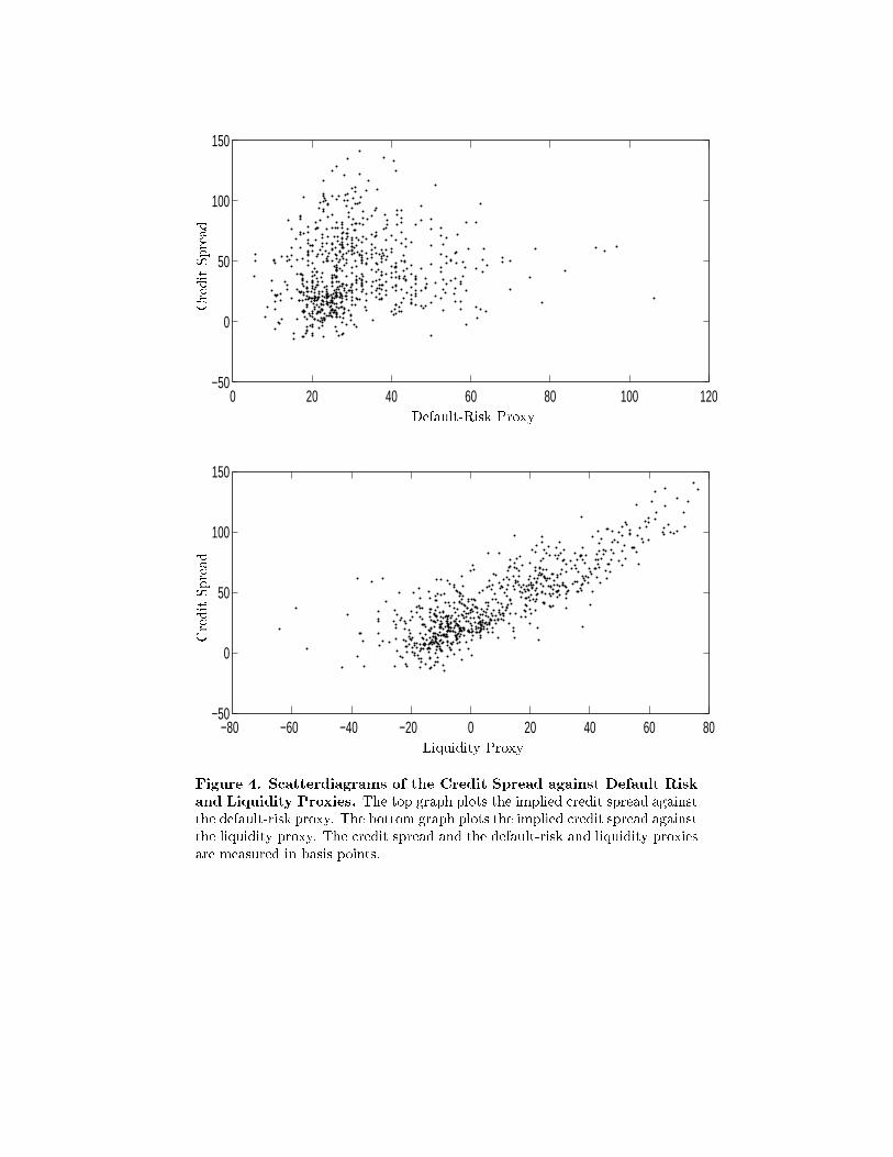
In theory, the spread λ could include both default-risk and liquidity components.Although there is no simple way to decompose the spread into these two components,it is interesting to compare the spread with several variables which may be correlatedwith these components. For example, the spread between the general repo rate and theimplied financing rate can be viewed as a proxy for Treasury liquidity. Similarly, thespread between the Libor rate and the general repo rate should contain informationabout the default risk of banks quoting Libor rates. To explore this, Fig. 4 presentsscatterdiagrams of the credit spread against these two variables. As illustrated, thecorrelation between the spread and the proxy for liquidity is much higher than thecorrelation between the spread and the proxy for default risk. In particular, thecorrelation of the spread with the default-risk proxy is .126 while the correlation ofthe spread with the liquidity proxy is .830. Furthermore, the correlation of weeklychanges in the spread with changes in in the default-risk proxy is -.115 while thecorrelation of weekly changes in the spread with changes in the liquidity proxy is .558.Taken together, these results are supportive of the view that much of the variation inspreads is driven by changes in liquidity.

7. THE MARKET PRICE OF CREDIT RISK

A major objective of this paper is to examine how the market prices the credit risk ininterest rate swaps. To this end, we focus on the premia that are incorporated intothe expected returns of bonds implied by the estimated term structure model. Thesepremia are given directly from the differences between the objective and risk-neutralparameters of the model.

To provide some perspective for these results, however, it is useful to also examinethe implications of the model for the term premia in Treasury bond prices. ApplyingIto’s Lemma to the closed-form expression for the value of a riskless zero-coupon bondgiven in Eq. (7) results in the following expression for its instantaneous expectedreturn

17

r + b (t)((β − κ)Xt + κθ)). (18)

The first term in this expression is the riskless rate and the sum of the remaining termsis the instantaneous term premium for the bond. This term premium is time varyingsince it depends explicitly on the state variables. To solve for the unconditional termpremium, we take the expectation over the objective measure of the state variableswhich gives b (t)βθ.

Now applying Ito’s Lemma to the closed-form expression for the price of therisky zero-coupon bond given in Eq. (8) leads to the following expression for theinstantaneous expected return

r + d (t)((β − κ)Xt + κθ)). (19)

The first term in this expression is again the instantaneous risky rate. The sum ofthe remaining terms can be interpreted as the combined term premium and creditpremium. To solve for the credit premium separately, we simply take the differencebetween the expected return of a risky zero-coupon bond and the expected return ona riskless zero-coupon bond with the same maturity. As before, the credit premiumis time varying through its dependence on the state variables. Taking the expectationwith respect to the objective measure for the state variables and subtracting theexpression for the unconditional term premium gives (d(t)− b(t)) βθ.

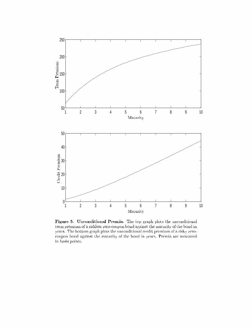
Focusing first on the unconditional premia, Table 7 reports the unconditionalterm premia for riskless zero-coupon bonds with maturities ranging from one to tenyears. Table 7 also reports the unconditional credit premia for risky zero-couponbonds with the same maturities. These unconditional premia are also graphed inFig. 5. As shown, the mean term premia are positive and monotonically increasingfunctions of time to maturity. Mean term premia range from about 97 basis points fora one-year horizon to about 321 basis points for a ten-year horizon. These estimatesof unconditional term premia are similar to those reported by Fama (1984), Fama andBliss (1987), and others.

Table 7 and Fig. 5 also show that unconditional credit premia are positive andincreasing functions of maturity. The mean credit premium for a one-year horizon isonly 0.1 basis points. Thus, there is very little compensation on average for bearingshort-term credit risk. At longer horizons, however, the mean credit premium is muchlarger. For example, the mean credit premium for a ten-year horizon is 45 basispoints. The convex shape of the unconditional credit premium curve indicates thatinvestors require sharply higher credit premia as the maturity of the bond increases.This pattern contrasts with that observed for the unconditional term premia.

To give some sense of the time variation in term and credit premia, Fig. 6 graphsthese premia for a ten-year maturity zero-coupon bond. As illustrated, the term

18

premium displays a significant amount of variation. The term premium is usuallypositive, but has generally tended downward throughout the sample period and issignificantly negative at the end of the sample period.

The time series of the credit premium displays a number of surprising features.Recall that the average credit premium for a ten-year horizon is about 45 basis points.Fig. 6 shows that the conditional credit premium varies significantly over time and isoften large in absolute terms. Most surprisingly, the credit premium is negative fornearly one half of the sample period. The credit premium first becomes negative inapproximately 1992 and remains generally negative until the fall of 1998. This is aboutwhen the Russian government defaulted on a large issue of its ruble-denominated debt.Despite the variation, however, the credit premium appears to be less volatile than theterm premium. Although not shown, a very similar pattern holds for credit premia inbonds with shorter maturities.

8. CONCLUSION

This paper examines how the market prices the credit and liquidity risk inherent ininterest rate swaps relative to Treasury bonds. A number of key results emerge fromthis analysis. For example, we find that on-the-run Treasury bonds have a significantliquidity component to their value. This liquidity component can be as much as 0.57percent of the notional amount of a ten-year Treasury bond. The value of this liquiditycomponent varies significantly over time. In addition, we find that the market pricesthe credit risk of swaps. The market price of credit risk, however, varies over time andwas occasionally negative for during the 1990s.

There are a number of possible extensions to this research. For example, theapproach of solving for the implied financing rate could be applied to the term struc-tures for corporate bond issuers and then used to identify the liquidity components oftheir spreads.15 One major puzzle is why the credit premia implicit in swap spreadswere negative during the 1990s, and only became significantly positive again afterthe hedge-fund crisis of 1998. Certainly, these results are difficult to reconcile with aview of the market in which investors are aware of the historical variability in swapspreads and where expected returns compensate investors for their exposure to risk.A possible resolution of this puzzle may be that most of the credit risk reflected inswap spreads may actually represent the liquidity risk of Treasury bonds. From thisperspective, Treasury bonds may be subject to a unique risk which does not affectpure contracts such as swaps, and may be priced accordingly in the market. Clearly,further research is necessary to resolve this issue.

15Huang and Huang (2000) focus on the estimation of the liquidity components incorporate bond prices.

19

REFERENCES

Amihud, Y. and H. Mendelson, 1991, Liquidity, Maturity, and the Yields on U. S.Treasury Securities, The Journal of Finance 46, 1411-1425.

Bicksler, J. and A. H. Chen, 1986, An Economic Analysis of Interest Rate Swaps,Journal of Finance 41, 645-655.

Black, F. and J. Cox, 1976, Valuing Corporate Securities: Some Effects of Bond Inden-ture Provisions, The Journal of Finance 31, 351-367.

Bollier, T., and E. Sorensen, 1994, Pricing Swap Default Risk, Financial Analysts Jour-nal, May-June, 23-33.

Boudoukh, J. and R. Whitelaw, 1993, Liquidity as a Choice Variable: A Lesson from theJapanese Government Bond Market, The Review of Financial Studies 6, 265-292.

Brown, K., W. Harlow, and D. Smith, 1994, An Empirical Analysis of Interest RateSwap Spreads, Journal of Fixed Income, March, 61-78.

Buraschi, A. and D. Menini, 2001, Liquidity Risk and Special Repos: How Well DoForward Repo Spreads Price Future Specialness, Journal of Financial Economics,forthcoming.

Chapman, D., J. Long, Jr., and N. Pearson, 1999, Using Proxies for the Short Rate:When are Three Months Like an Instant?, Review of Financial Studies 12, 763-806.

Chapman, D., and N. Pearson, 2001, Recent Advances in Estimating Term-StructureModels, Financial Analysts Journal July/August, 77-95.

Chen, R. R. and L. Scott, 1993, Maximum Likelihood Estimation for a MultifactorEquilibrium Model of the Term Structure of Interest Rates, Journal of Fixed Income3, 14-31.

Collin-Dufresne, P. and B. Solnik, 2001, On the Term Structure of Default Premia inthe Swap and Libor Markets, The Journal of Finance, forthcoming.

Cooper, I. and A. Mello, 1991, The Default Risk on Swaps, The Journal of Finance 46,597-620.

Dai, Q. and K. Singleton, 2000, Specification Analysis of Affine Term Structure Models,The Journal of Finance 55, 1943-1978.

Dai, Q. and K. Singleton, 2001, Expectations Puzzles, Time-Varying Risk Premia, andDynamic Models of the Term Structure, Journal of Financial Economics, forthcom-ing.

Dai, Q. and K. Singleton, 2002, Term Structure Dynamics in Theory and Reality, Work-ing Paper, Stanford University.

Duffee, G., 1996, Idiosyncratic Variation of Treasury Bill Yield Spreads, Journal ofFinance 51, 527-552.

Duffee, G., 1998, The Relation Between Treasury Yields and Corporate Bond YieldSpreads, Journal of Finance 53, 2225-2241.

Duffee, G., 1999, Estimating the Price of Default Risk, The Review of Financial Studies12, 197-226.

Duffee, G., 2002, Term Premia and Interest Rate Forecasts in Affine Models, Journalof Finance 57, 405-443.

Duffie, D., 1996, Special Repo Rates, The Journal of Finance 51, 493-526.

Duffie, D. and M. Huang, 1996, Swap Rates and Credit Quality, The Journal of Finance51, 921-949.

Duffie, D. and R. Kan, 1996, A Yield-Factor Model of Interest Rates, MathematicalFinance 6, 379-406.

Duffie, D. and J. Liu, 2001, Floating-Fixed Credit Spreads, Financial Analysts Journal57, May/June, 76-87.

Duffie, D., L. Pedersen, K. Singleton, 2000, Modeling Sovereign Yield Spreads: A CaseStudy of Russian Debt, Working paper, Stanford University.

Duffie, D. and K. Singleton, 1997, An Econometric Model of the Term Structure ofInterest Rate Swap Spreads, The Journal of Finance 52, 1287-1321.

Duffie, D. and K. Singleton, 1999, Modeling Term Structures of Defaultable Bonds, TheReview of Financial Studies 12, 687-720.

Fama, E. , 1984, Term Premiums in Bond Returns, Journal of Financial Economics 13,529-546.

Fama, E. and R. Bliss, 1987, The Information in Long-Maturity Forward Rates, Amer-ican Economic Review 77, 680-692.

Grinblatt, M., 2001, An Analytical Solution for Interest Rate Swap Spreads, Review ofInternational Finance, forthcoming.

Gupta, A. and M. Subrahmanyam, 2000, An Empirical Investigation of the ConvexityBias in the Pricing of Interest Rate Swaps, Journal of Financial Economics 55,239-279.

He, H., 2000, Modeling Term Structures of Swap Spreads, Working paper, Yale Univer-sity.

Huang, J., and M. Huang, 2000, How Much of the Corporate-Treasury Yield Spreadis Due to Credit Risk?: Results from a New Calibration Approach, Working paper,Stanford University.

Jordan, B. and S. Jordan, 1997, Special Repo Rate: An Empirical Analysis, The Journalof Finance 52, 2051-2072.

Kamara, A., 1994, Liquidity, Taxes, and Short-Term Treasury Yields, Journal of Fi-nancial and Quantitative Analysis 29, 403-417.

Knez, P., R. Litterman, and J. Scheinkman, 1994, Explorations into Factors ExplainingMoney Market Returns, The Journal of Finance 49, 1861-1882.

Krishnmurthy, A., 2001, The Bond/Old-Bond Spread, Working paper, NorthwesternUniversity.

Litterman, R. and J. Scheinkman, 1991, Common Factors Affecting Bond Returns, TheJournal of Fixed Income 1, 54-61.

Litzenberger, R., 1992, Swaps: Plain and Fanciful, The Journal of Finance 42, 831-850.

Longstaff, F., 2000, The Term Structure of Very Short-Term Rates: New Evidence forthe Expectations Hypothesis, Journal of Financial Economics 58, 397-415.

Longstaff, F. and E. Schwartz, 1992, Interest Rate Volatility and the Term Structure:A Two-Factor General Equilibrium Model, The Journal of Finance 47, 1259-1282.

Longstaff, F. and E. Schwartz, 1995, A Simple Approach to Valuing Risky Fixed andFloating Rate Debt, The Journal of Finance 50, 789-819.

Longstaff, F., P. Santa-Clara, and E. S. Schwartz, 2001, The Relative Valuation of Capsand Swaptions: Theory and Empirical Evidence, Journal of Finance 56, 2067-2109.

Macfarlane, J., D. Ross, and J. Showers, 1991, The Interest Rate Swap Market: YieldMathematics, Terminology, and Conventions, in Interest Rate Swaps, ed. Carl R.Beidleman, (Business One Irwin, Homewood, IL).

Merton, R. C., 1974, On the Pricing of Risky Debt: The Risk Structure of InterestRates, The Journal of Finance 29, 449-470.

Minton, B., 1997, An Empirical Examination of Basic Valuation Models for Plain VanillaU.S. Interest Rate Swaps, Journal of Financial Economics 44, 251-277.

Pearson, N. and T-S. Sun, 1994, An Empirical Examination of the Cox, Ingersoll, and

Ross Model of the Term Structure of Interest Rates Using the Method of MaximumLikelihood, The Journal of Finance 54, 929-959.

Piazzesi, M., 1999, An Econometric Model of the Yield Curve with MacroeconomicJump Effects, Working paper, UCLA.

Smith, C. W., C. W. Smithson, and L. M. Wakeman, 1988, The Market for InterestRate Swaps, Financial Management 17, 34-44.

Sun, T., S. M. Sundaresan, and C. Wang, 1993, Interest Rate Swaps: An EmpiricalInvestigation, Journal of Financial Economics 36, 77-99.

Sundaresan, S. M., 1991, Valuation of Swaps, in Sarkis J. Khoury, ed., Recent Devel-opments in International Banking and Finance, vol 5, New York: Elsevier SciencePublishers.

Sundaresan, S. M., 1994, An Empirical Analysis of U.S. Treasury Auctions: Implicationsfor Auction and Term Structure Theories, Journal of Fixed Income, 35-50.

Turnbull, S., 1987, Swaps: Zero-Sum Game?, Financial Management 16, 15-21.

Vasicek, O., 1977, An Equilibrium Characterization of the Term Structure, Journal ofFinancial Economics 5, 177-188.

Wall, L. D. and J. J. Pringle, 1989, Alternative Explanations of Interest Rate Swaps:A Theoretical and Empirical Analysis, Financial Management 16, 15-21

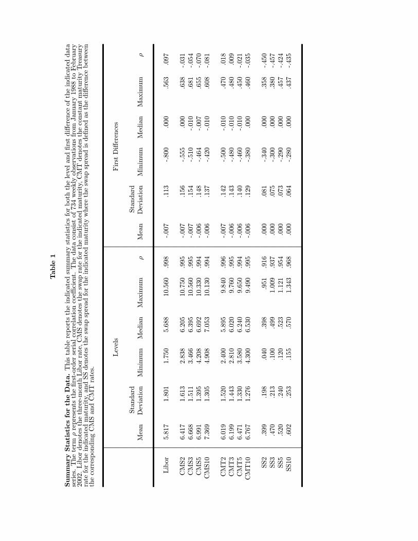
Table1

SummaryStatisticsfortheData.Thistablereportstheindicatedsummarystatisticsforboththelevelandfirstdifferenceoftheindicateddata

series.Theterm

ρrepresentsthefirst-orderserialcorrelationcoefficient.Thedataconsistof734weeklyobservationsfrom

January1988toFebruary

2002.Libordenotesthethree-monthLiborrate,CMSdenotestheswapratefortheindicatedmaturity,CMTdenotestheconstantmaturityTreasury

ratefortheindicatedmaturity,andSSdenotestheswapspreadfortheindicatedmaturitywheretheswapspreadisdefinedasthedifferencebetween

thecorrespondingCMSandCMTrates.

Levels

FirstDifferences

Standard

Standard

Mean

Deviation

Minimum

Median

Maximum

ρMean

Deviation

Minimum

Median

Maximum

ρ

Libor

5.817

1.801

1.750

5.688

10.560

.998

-.007

.113

-.800

.000

.563

.097

CMS2

6.417

1.613

2.838

6.205

10.750

.995

-.007

.156

-.555

.000

.638

-.031

CMS3

6.668

1.511

3.466

6.395

10.560

.995

-.007

.154

-.510

-.010

.681

-.054

CMS5

6.991

1.395

4.208

6.692

10.330

.994

-.006

.148

-.464

-.007

.655

-.070

CMS10

7.369

1.305

4.908

7.053

10.130

.994

-.006

.137

-.420

-.010

.608

-.081

CMT2

6.019

1.520

2.400

5.895

9.840

.996

-.007

.142

-.500

-.010

.470

.018

CMT3

6.199

1.443

2.810

6.020

9.760

.995

-.006

.143

-.480

-.010

.480

.009

CMT5

6.471

1.330

3.580

6.240

9.650

.994

-.006

.140

-.460

-.010

.450

-.021

CMT10

6.767

1.276

4.300

6.530

9.490

.995

-.006

.129

-.380

.000

.460

-.035

SS2

.399

.198

.040

.398

.951

.916

.000

.081

-.340

.000

.358

-.450

SS3

.470

.213

.100

.499

1.009

.937

.000

.075

-.300

.000

.380

-.457

SS5

.520

.240

.120

.523

1.121

.954

.000

.073

-.290

.000

.457

-.424

SS10

.602

.253

.155

.570

1.343

.968

.000

.064

-.280

.000

.437

-.435

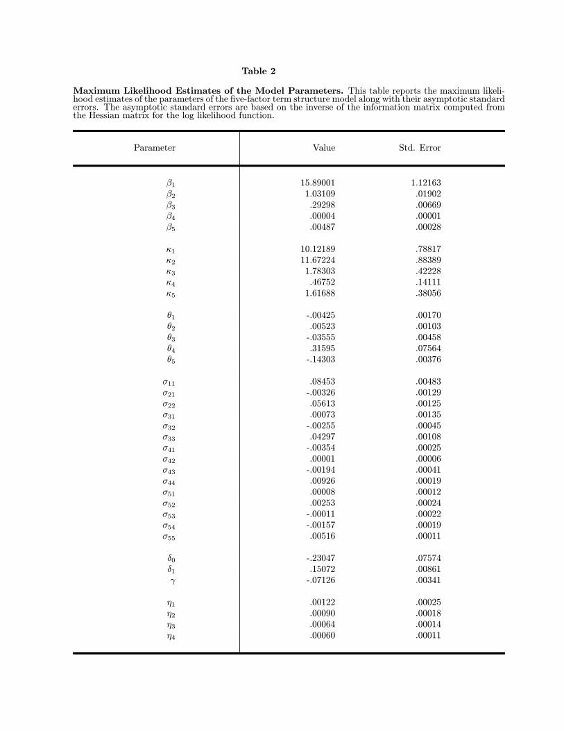
Table 2

Maximum Likelihood Estimates of the Model Parameters. This table reports the maximum likeli-hood estimates of the parameters of the five-factor term structure model along with their asymptotic standarderrors. The asymptotic standard errors are based on the inverse of the information matrix computed fromthe Hessian matrix for the log likelihood function.

Parameter Value Std. Error

β1 15.89001 1.12163β2 1.03109 .01902β3 .29298 .00669β4 .00004 .00001β5 .00487 .00028

κ1 10.12189 .78817κ2 11.67224 .88389κ3 1.78303 .42228κ4 .46752 .14111κ5 1.61688 .38056

θ1 -.00425 .00170θ2 .00523 .00103θ3 -.03555 .00458θ4 .31595 .07564θ5 -.14303 .00376

σ11 .08453 .00483σ21 -.00326 .00129σ22 .05613 .00125σ31 .00073 .00135σ32 -.00255 .00045σ33 .04297 .00108σ41 -.00354 .00025σ42 .00001 .00006σ43 -.00194 .00041σ44 .00926 .00019σ51 .00008 .00012σ52 .00253 .00024σ53 -.00011 .00022σ54 -.00157 .00019σ55 .00516 .00011

δ0 -.23047 .07574δ1 .15072 .00861γ -.07126 .00341

η1 .00122 .00025η2 .00090 .00018η3 .00064 .00014η4 .00060 .00011

Table 3

Correlation Matrix for the State Variables. This table reports the instantaneous correlationmatrix for the state variable vector implied by the maximum likelihood estimates of the parametersin Table 2.

X1 X2 X3 X4 X5

X1 1.0000

X2 -.0579 1.0000

X3 .0169 -.0602 1.000

X4 -.3505 .0209 -.1972 1.0000

X5 .0132 .4226 -.0440 -.2422 1.0000

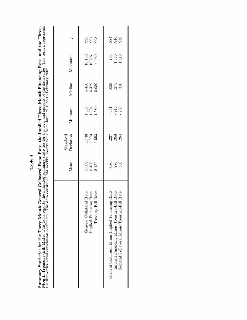
Table4

SummaryStatisticsfortheThree-MonthGeneralCollateralRepoRate,theImpliedThree-MonthFinancingRate,andtheThree-

MonthTreasury-BillRate.Thistablereportstheindicatedsummarystatisticsforthelevelandspreadsofthedataseries.Theterm

ρrepresents

thefirst-orderserialcorrelationcoefficient.Thedataconsistof734weeklyobservationsfrom

January1988toFebruary2002.

Standard

Mean

Deviation

Minimum

Median

Maximum

ρ

GeneralCollateralRate

5.509

1.748

1.560

5.450

10.150

.998

ImpliedFinancingRate

5.428

1.773

1.004

5.479

10.297

.997

Treasury-BillRate

5.152

1.553

1.580

5.050

9.030

.998

GeneralCollateralMinusImpliedFinancingRate

.080

.237

-.641

.029

.764

.884

ImpliedFinancingMinusTreasury-BillRate

.276

.358

-.716

.275

1.556

.946

GeneralCollateralMinusTreasury-BillRate

.356

.264

-.200

.310

1.410

.930

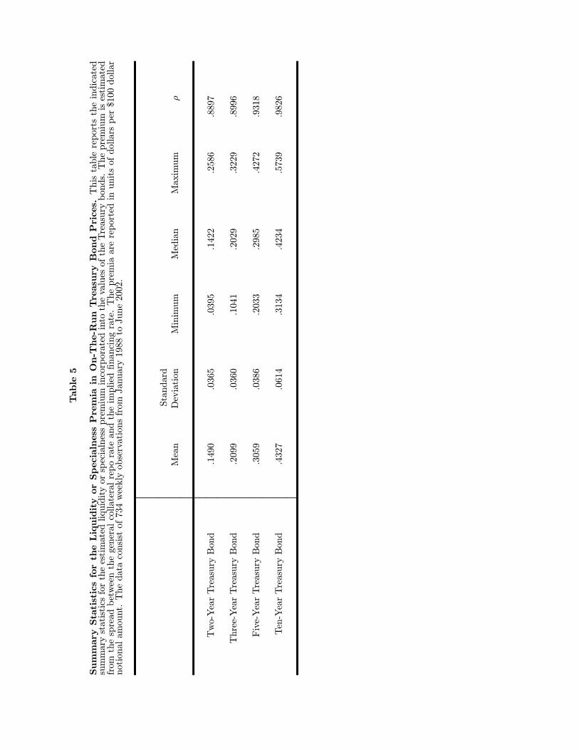
Table5

Summary

StatisticsfortheLiquidityorSpecialnessPremiainOn-The-RunTreasury

BondPrices.Thistablereportstheindicated

summarystatisticsfortheestimatedliquidityorspecialnesspremiumincorporatedintothevaluesoftheTreasurybonds.Thepremiumisestimated

from

thespreadbetweenthegeneralcollateralreporateandtheimpliedfinancingrate.Thepremiaarereportedinunitsofdollarsper$100dollar

notionalamount.Thedataconsistof734weeklyobservationsfrom

January1988toJune2002.

Standard

Mean

Deviation

Minimum

Median

Maximum

ρ

Two-YearTreasuryBond

.1490

.0365

.0395

.1422

.2586

.8897

Three-YearTreasuryBond

.2099

.0360

.1041

.2029

.3229

.8996

Five-YearTreasuryBond

.3059

.0386

.2033

.2985

.4272

.9318

Ten-YearTreasuryBond

.4327

.0614

.3134

.4234

.5739

.9826

Table6

SpecialandGeneralCollateralTerm

RepoRatesandtheImpliedSpecialnessPremiaforTreasuryBondsasofJune30,2000.This

tablereportsthelongestquotedterm

specialreporatesfortheindicatedTreasurybondsalongwiththecorrespondingterm

generalcollateralrepo

rate.Theimpliedspecialnessiscomputedbymultiplyingthedifferencebetweenthetworatesbytheterm

ofthereporatesmeasuredinyearsand

representsthespecialnesspremiumper$100value.Theon-the-runissuesaredenotedbyanasterisk.

LongestRepo

GeneralCollateral

SpecialTerm

Implied

Coupon

Maturity

TerminDays

TermRepoRate

RepoRate

Difference

Specialness

5.875

30-Nov-01

92.06461

.06450

.00011

.003

6.625

31-May-02

78.06424

.06050

.00374

.080

6.375∗

30-Jun-02

32.06346

.05550

.00796

.070

5.250

15-Aug-03

92.06461

.06400

.00061

.016

4.250

15-Nov-03

286

.06714

.06650

.00064

.050

4.750

15-Feb-04

92.06461

.06350

.00111

.028

6.000

15-Aug-04

92.06461

.06400

.00061

.016

5.875

15-Nov-04

92.06461

.06300

.00161

.041

6.750∗

15-May-05

358

.06765

.06250

.00515

.505

6.500

15-May-05

93.06462

.06350

.00112

.029

5.625

15-Feb-06

93.06462

.06400

.00062

.016

6.875

15-May-06

93.06462

.06400

.00062

.016

7.000

15-Jul-06

93.06462

.06350

.00112

.029

6.500

15-Oct-06

93.06462

.06400

.00062

.016

6.250

15-Feb-07

92.06461

.06400

.00061

.015

6.625

15-May-07

93.06462

.06400

.00062

.016

6.125

15-Aug-07

93.06462

.06400

.00062

.016

5.500

15-Feb-08

93.06462

.06400

.00062

.016

5.625

15-May-08

93.06462

.06400

.00062

.016

4.750

15-Nov-08

183

.06592

.06500

.00092

.046

5.500

15-May-09

259

.06687

.06600

.00087

.062

6.000

15-Aug-09

298

.06724

.06600

.00124

.101

6.250∗

15-Feb-10

354

.06763

.06100

.00663

.643

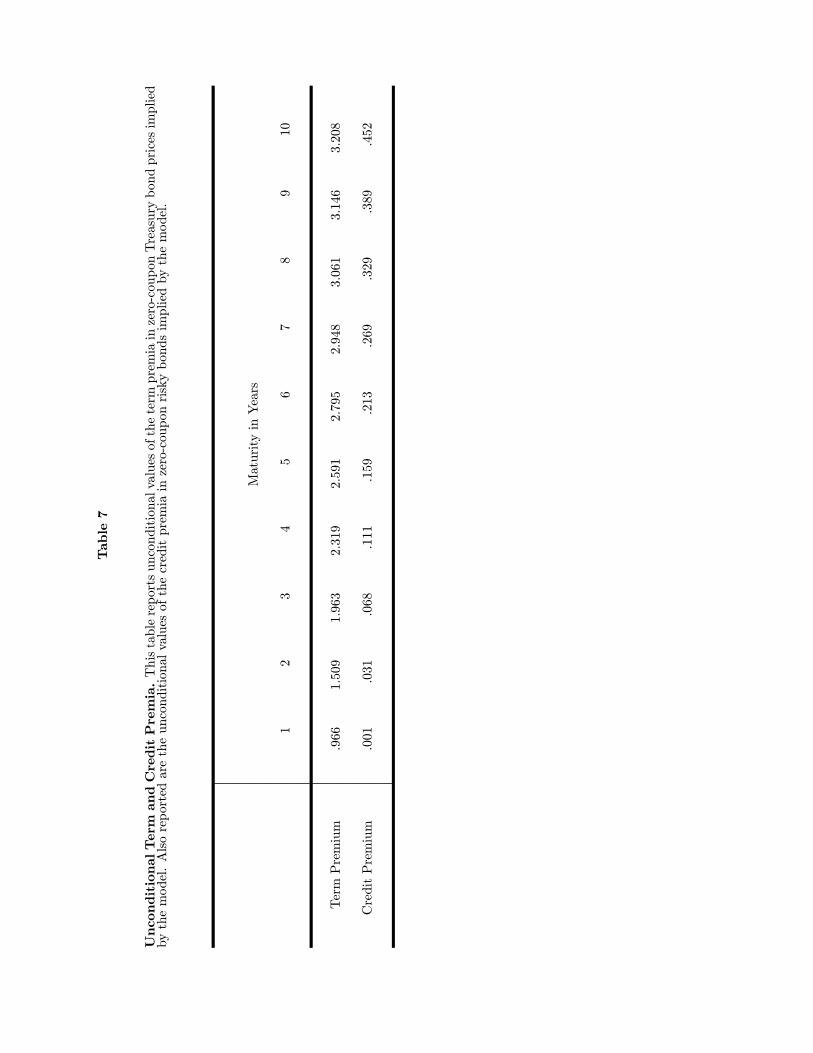
Table7

UnconditionalTerm

andCreditPremia.Thistablereportsunconditionalvaluesofthetermpremiainzero-couponTreasurybondpricesimplied

bythemodel.Alsoreportedaretheunconditionalvaluesofthecreditpremiainzero-couponriskybondsimpliedbythemodel.

MaturityinYears

12

34

56

78

910

TermPremium

.966

1.509

1.963

2.319

2.591

2.795

2.948

3.061

3.146

3.208

CreditPremium

.001

.031

.068

.111

.159

.213

.269

.329

.389

.452

88 90 92 94 96 98 00 020

50

100

150

88 90 92 94 96 98 00 020

50

100

150

88 90 92 94 96 98 00 020

50

100

150

88 90 92 94 96 98 00 020

50

100

150

88 90 92 94 96 98 00 02

−50

0

50

100

150

88 90 92 94 96 98 00 02

−50

0

50

100

150

! " #

$%!

&' ( )

( ' $% &' (

88 90 92 94 96 98 00 02

0

20

40

60

80

100

120

140

!

' '

0 20 40 60 80 100 120−50

0

50

100

150

−80 −60 −40 −20 0 20 40 60 80−50

0

50

100

150

*# +,

- . +,

%

%

! "# ( ' (

, ( ' (

. , ' . ,

1 2 3 4 5 6 7 8 9 1050

100

150

200

250

1 2 3 4 5 6 7 8 9 100

10

20

30

40

50

/

/

+

% +

$ % " ( '

0' (

( ' ' 0

' ( +

88 90 92 94 96 98 00 02

−0.3

−0.2

−0.1

0

0.1

0.2

0.3

0.4

88 90 92 94 96 98 00 02

−0.05

0

0.05

0.1

+

% +

& " ( '

0' (

' ' 0'