NBER WORKING PAPER SERIES

THE FINANCE UNCERTAINTY MULTIPLIER

Iván AlfaroNicholas Bloom

Xiaoji Lin

Working Paper 24571http://www.nber.org/papers/w24571

NATIONAL BUREAU OF ECONOMIC RESEARCH1050 Massachusetts Avenue

Cambridge, MA 02138May 2018

We would like to thank our formal discussants Nicolas Crouzet, Ian Dew-Becker, Simon Gilchrist, Po-Hsuan Hsu, Howard Kung, Gill Segal, Toni Whited, and the seminar audiences at the Adam Smith Conference, AEA, AFA, Beijing University, BI Norwegian Business School, CEIBS, Econometric Society, European Finance Association, Macro Finance Society Workshop, Melbourne Institute Macroeconomic Policy Meetings, Midwest Finance Association, Minneapolis Fed, NY Fed, Society for Nonlinear Dynamics and Econometrics, Stanford, The Ohio State University, UBC Summer Finance Conference, University College London, University of North Carolina at Chapel Hill, University of St. Andrews, University of Texas at Austin, University of Texas at Dallas, University of Toronto, Utah Winter Finance Conference, World Congress. The NSF and Alfred Sloan Foundation kindly provided research support. The views expressed herein are those of the authors and do not necessarily reflect the views of the National Bureau of Economic Research.

NBER working papers are circulated for discussion and comment purposes. They have not been peer-reviewed or been subject to the review by the NBER Board of Directors that accompanies official NBER publications.

© 2018 by Iván Alfaro, Nicholas Bloom, and Xiaoji Lin. All rights reserved. Short sections of text, not to exceed two paragraphs, may be quoted without explicit permission provided that full credit, including © notice, is given to the source.

The Finance Uncertainty MultiplierIván Alfaro, Nicholas Bloom, and Xiaoji LinNBER Working Paper No. 24571May 2018JEL No. E0,G0

ABSTRACT

We show how real and financial frictions amplify the impact of uncertainty shocks. We build a model with real frictions, and find adding financial frictions roughly doubles the impact of uncertainty shocks. Higher uncertainty alongside financial frictions induces the standard real-options effects on investment and hiring, but also leads firms to hoard cash, further reducing investment and hiring. We then test the model using a panel of US firms and a novel instrumentation strategy for uncertainty exploiting differential firm exposure to exchange rate and price volatility. These results highlight why in periods with greater financial frictions uncertainty can be particularly damaging.

Iván AlfaroDepartment of FinanceBI Norwegian Business School Nydalsveien 37N-0484 OsloNorwayivan.alfaro@bi.no

Nicholas BloomStanford University Department of Economics 579 Serra MallStanford, CA 94305-6072 and NBERnbloom@stanford.edu

Xiaoji LinDepartment of FinanceOhio State University2100 Neil AveColumbus, OH 43210lin.1376@osu.edu

1 Introduction

This paper seeks to address two related questions. First, why are uncertainty shocks in some

periods - like the 2007-2009 global financial crisis - associated with large drops in output, while

in other periods - like the Brexit vote or 2016 US election - are accompanied by economic

growth? Second, as Stock and Watson (2012) noted, uncertainty shocks and financial shocks

are highly correlated. Are these the same shock, or are they distinct shocks with an interrelated

impact, in which uncertainty is amplified by financial frictions?

To address these questions we build a heterogeneous firms dynamic model with two key

extensions. First, real and financial frictions: on the real side investment incurs fixed cost,1 and

on the financing side issuing equity involves a fixed cost.2 Second, uncertainty and financing

costs are both stochastic, with large temporary shocks. The model is calibrated, solved and

then simulated as a panel of heterogeneous firms.

We show two key results. Our first key result is a Finance Uncertainty Multiplier

(hereafter FUM). Namely, adding financial frictions to the classical model of stochastic-

volatility uncertainty shocks - as in Dixit and Pindyck (1994), Abel and Eberly (1996) or

Bloom (2009) - roughly doubles the negative impact of uncertainty shocks on investment and

hiring. In our simulation an uncertainty shock with real and financial frictions leads to a peak

drop in output of 2.3%, but with only real frictions a drop of 1.2%. So, introducing financial

costs roughly doubles the impact of uncertainty shocks on output.

Our second key result is that uncertainty shocks and financial shocks have an almost

additive impact on output. In our simulations, uncertainty shocks or financial shocks in

models with real and financial frictions each individually reduce output by 2.3% and 2.1%

respectively, but jointly reduce output by 3.5%.

We summarize these two results below. This reports the peak drop in aggregate output in

our calibrated model with only real frictions and an uncertainty shock is 1.2% (top left box).

1For example, Bertola and Caballero (1990), Davis and Haltiwanger (1992), Dixit and Pindyck (1994),Caballero, Engel, and Haltiwanger (1995), Abel and Eberly (1996), or Cooper and Haltiwanger (2006).

2See, for example, Hennessy and Whited (2005), Hennessy and Whited (2007), Bolton, Chen, and Wang(2013), Eisfeldt and Muir (2016), etc.

2

Adding financial frictions almost doubles the size of an uncertainty shock to 2.3% (bottom left

box). Finally, adding a financial shock (as well as an uncertainty shock) increases the impact

by another one half, yielding a drop in output of 3.5% (bottom right). So collectively going

from the classic uncertainty model to one with financial frictions and simultaneous financial

shocks roughly triples the impact of uncertainty shocks, and can help explain why uncertainty

shocks during periods like 2007-2009 were associated with large drops in output.

Key results in simulation

Uncertainty Uncertainty

shock + financial shocks

Real frictions 1.2% n/a

Real+financial frictions 2.3% 3.5%

Notes: Results from simulations of 30,000 firms in the calibrated model (see section 3.4.1).

Alongside the negative impact of uncertainty and finance shocks on investment and

employment, the model also predicts these shocks will lead firms to accumulate cash and

reduce equity payouts, as higher uncertainty causes firms to take a more cautious financial

position. As Figure 1 shows this is consistent with macro-data. It plots the quarterly VIX

index - a common proxy for uncertainty - alongside aggregate real and financial variables.

The top two panels show that times of high uncertainty (VIX) are associated with periods of

low investment and employment growth. The middle two panels show that cash holding is

positively associated with the VIX, while dividend payout and equity repurchase are negatively

related to the VIX. The bottom panels also considers debt and shows that the total debt (the

sum of the short-term and long-term debt) growth and the term structure of the debt growth

(short-term debt growth to long-term debt growth ratio) are both negatively related with the

VIX, implying firms cut debt (and particularly short-term debt) when uncertainty is high.

The additional complexity required to model: (a) real and financial frictions, and (b)

uncertainty and financial shocks, required us to make some simplifying assumptions. First, we

ignore labor adjustment costs - including these would likely increase the impact of uncertainty

shocks, since labor accounts for 2/3 of the cost share in our model. Second, we ignore general

3

equilibrium (GE) effects - including these would likely reduce the impact of uncertainty shocks

by allowing for offsetting price effects. As a partial response to this we also run a pseudo-GE

robustness test where we allow interest rates, prices (of output and capital) and real wages

to move after uncertainty shocks following typical changes observed in the data, and find our

results on the negative impact of uncertainty-finance shocks on output are about 30% smaller

but qualitatively similar.3

The second part of the paper tests this model using a micro-data panel of US firms with

measures of uncertainty, investment, employment, cash, debt and equity payments. To address

obvious concerns over endogeneity of uncertainty4 we employ a novel instrumentation strategy

for uncertainty exploiting differential firm exposure to exchange rate, factor price and policy

uncertainty. This identification strategy works well delivering a strong first-stage F-statistics

and passing Hansen over-identification tests. We find that higher uncertainty significantly

reduces investment (in tangible and intangible capital) and hiring, while also leading firms

to more cautiously manage their financial polices by increasing cash holdings and cutting

dividends, debt, and stock-buy backs, consistent with the model (and macro data).

Our paper relates to three main literatures. First, the large uncertainty literature studying

the impact of heightened uncertainty and volatility on investment and employment.5 We build

on this literature to show the joint importance of real and financial frictions for investment,

3One reason is that wages and real interest rates do not move substantially over the cycle (e.g. King andRebelo (1999)), and second increased uncertainty widens the Ss bands so that the economy is less responsiveto price changes (e.g. Bloom, Floetotto, Jaimovich, Saporta-Eksten, and Terry (2016)).

4See, for example, Nieuwerburgh and Veldkamp (2006), Bachmann and Moscarini (2012), Pastor andVeronesi (2012), Orlik and Veldkamp (2015), Berger, Dew-Becker, and Giglio (2016), and Falgelbaum, Schaal,and Taschereau-Dumouchel (2016), for models and empirics on reverse causality with uncertainty and growth.

5Classic papers on uncertainty and growth included Bernanke (1983), Romer (1990), Ramey and Ramey(1995), Leahy and Whited (1996), Guiso and Parigi (1999), Bloom (2009), Bachmann and Bayer (2013),Fernandez-Villaverde, Quintana, Rubio-Ramirez, and Uribe (2011), Fernandez-Villaverde, Guerron-Quintana,Kuester, and Rubio-Ramirez (2015), and Christiano, Motto, and Rostagno (2014). Several other papers look atuncertainty shocks - for example, Bansal and Yaron (2004) and Segal, Shaliastovich, and Yaron (2015) look atthe consumption and financial implications of uncertainty, Handley and Limao (2012) look at uncertainty andtrade, Ilut and Schneider (2014) model ambiguity aversion as an alternative to stochastic volatility, and Basuand Bundick (2017) examine uncertainty shocks in a sticky-price Keynesian model, and Berger, Dew-Becker,and Giglio (2016) study news vs uncertainty. A related literature on disaster shocks - for example, Rietz(1988), Barro (2006), and Gourio (2012) - is also connected to this paper, in that disasters can be interpretedas periods of combined uncertainty and financial shocks, and indeed can lead to uncertainty through beliefupdating (e.g. Orlik and Veldkamp (2015)).

4

hiring and financial dynamics, and importantly how adding financial shocks can roughly double

the impact of uncertainty shocks.

Second, the literature on financial frictions and business cycles.6 We build on this literature

to argue it is not a choice between uncertainty shocks and financial shocks as to which

drives recessions, but instead these shocks amplify each other so they cannot be considered

individually.

Finally, the finance literature that studies the determinants of corporate financing choices.7

We are complementary to these studies by showing that uncertainty shocks have significant

impact on firms’ real and financial flows, examined in both calibrated macro models and well

identified micro-data estimations.

The rest of the paper is laid out as follows. In section 2 we write down the model. In

section 3 we present the main quantitative results of the model. In section 4 we describe the

instrumentation strategy and international data that we use in the paper. In section 5 we

present the empirical findings on the effects of uncertainty shocks on both real and financial

activity of firms. Section 6 concludes.

2 Model

The model features a continuum of heterogeneous firms facing uncertainty shocks and financial

frictions. Furthermore, financial adjustment costs vary over time and across firms. Firms

choose optimal levels of physical capital investment, labor, and cash holding each period to

maximize the market value of equity.

6For example, Alessandri and Mumtaz (2016) and Lhuissier and Tripier (2016) show in VAR estimates astrong interaction effect of financial constraints on uncertainty. More generally, Gilchrist and Zakrajsek (2012),Jermann and Quadrini (2012), Christiano, Motto, and Rostagno (2014), and Gilchrist, Sim, and Zakrajsek(2014), Arellano, Bai, and Kehoe (2016), show that financial frictions are important to explain the aggregatefluctuations for the recent financial crisis. Caggiano et al (2017) show that uncertainty shocks have a biggerimpact during recessions.

7For example, Rajan and Zingales (1995), Gomes (2001), Welch (2004), Moyen (2004), Hennessy andWhited (2005), Riddick and Whited (2009), DeAngelo, DeAngelo, and Whited (2011), Bolton, Chen, andWang (2011), Rampini and Viswanathan (2013), Chen, Wang, and Zhou (2014), and Chen (2016) study theimpact of various frictions on firms’ financing policies, including equity, debt, liquidity management, etc.

5

2.1 Technology

Firms use physical capital (Kt) and labor (Lt) to produce a homogeneous good (Yt). To save

on notation, we omit the firm index whenever possible. The production function is Cobb-

Douglas, given by

Yt = ZtKαt L

1−αt , (1)

in which Zt is firms’ productivity. The firm faces an isoelastic demand curve with elasticity

(ε),

Qt = BP−εt , (2)

where B is a demand shifter. These can be combined into a revenue function

R (Zt, B,Kt, Lt) = Z1−1/εt B1/εK

α(1−1/ε)t (Lt)

(1−α)(1−1/ε) . For analytical tractability we define

a = α (1− 1/ε) and b = (1− α) (1− 1/ε) , and substitute Z1−a−bt = Z

1−1/εt B1/ε. With these

redefinitions we have

S (Zt, Kt, Lt) = Z1−a−bt Ka

t Lbt . (3)

Wages are normalized to 1 denoted as W . Given employment is flexible, we can obtain optimal

labor.8 Note that labor can be pre-optimized out even with financial frictions which will be

discussed later.

Productivity is defined as a firm-specific productivity process, following an AR(1) process

zt+1 = ρzzt + σtεzt+1 (4)

in which zt+1 = log(Zt+1), εzt+1 is an i.i.d. standard normal shock (drawn independently across

firms), and ρz, and σt are the autocorrelation and conditional volatility of the productivity

process.

The firm stochastic volatility process is assumed for simplicity to follow a two-point Markov

8Pre-optimized labor is given by(bWZ1−a−bt Ka

t

) 11−b .

6

chains

σt ∈ {σL, σH} ,where Pr (σt+1 = σj|σt = σk) = πσk,j. (5)

Physical capital accumulation is given by

Kt+1 = (1− δ)Kt + It, (6)

where It represents investment and δ denotes the capital depreciation rate.

We assume that capital investment entails nonconvex adjustment costs, denoted as Gt,

which are given by:

Gt = ckSt1{It 6=0}, (7)

where ck > 0 is constant. The capital adjustment costs include planning and installation costs,

learning to use the new equipment, or the fact that production is temporarily interrupted.

The nonconvex costs ckSt1{It 6=0} capture the costs of adjusting capital that are independent

of the size of the investment.

We also assume that there is a fixed production cost F ≥ 0. Firms need to pay this cost

regardless of investment and hiring decisions every period. Hence firms’ operating profit (Πt)

is revenue minus wages and fixed cost of production, given by

Πt = St − WLt − F. (8)

2.2 Cash holding

Firms save in cash (Nt+1) which represents the liquid asset that firms hold. Cash accumulation

evolves according to the process

Nt+1 = (1 + rn)Nt +Ht, (9)

7

where Ht is the investment in cash and rn > 0 is the return on holding cash. Following

Cooley and Quadrini (2001) and Hennessy, Levy, and Whited (2007), we assume that return

on cash is strictly less than the risk free rate rf (i.e., rn < rf ). This assumption is consistent

with Graham (2000) who documents that the tax rates on cash retentions generally exceed

tax rates on interest income for bondholders, making cash holding tax-disadvantaged. Lastly,

cash is freely adjusted.

2.3 External financing costs

When the sum of investment in capital, investment adjustment cost and investment in cash

exceeds the operating profit, firms can take external funds by issuing equity. External equity

financing is costly for firms. The financing costs include both direct costs (for example,

flotation costs - underwriting, legal and registration fees), and indirect (unobserved) costs due

to asymmetric information and managerial incentive problems, among others.9

Because equity financing costs will be paid only if payouts are negative, we define the

firm’s payout before financing cost (Et) as operating profit minus investment in capital and

cash accumulation, less investment adjustment costs

Et = Πt − It −Ht −Gt. (10)

Furthermore, external equity financing costs vary over time and across firms.10 The micro-

foundations of time-varying financing conditions include endogenous time-varying adverse

selection problems in Eisfeldt (2004), Kurlat (2013), and Bigio (2015) who show that

uncertainty increases the adverse selection cost from equity offerings (raising financing costs),

9These costs are estimated to be substantial. For example, Altinkilic and Hansen (2000) estimate theunderwriting fee ranging from 4.37% to 6.32% of the capital raised in their sample. In addition, a fewempirical papers also seek to establish the importance of the indirect costs of equity issuance. Asquith andMullins (1986) find that the announcement of equity offerings reduces stock prices on average by −3% andthis price reduction as a fraction of the new equity issue is on average −31%.

10Erel, Julio, Kim, and Weisbach (2012) show that firms’ access to external finance markets also changeswith macroeconomic conditions. Kahle and Stulz (2013) find that net equity issuance falls more substantiallythan debt issuance during the recent financial crisis suggesting that shocks to the corporate credit supply arenot likely to be the cause for the reduction in firms’ capital expenditures in 2007-2008.

8

agency frictions varying over time as in Bernanke and Gertler (1989) and Carlstrom and

Fuerst (1997), and time-varying liquidity as in Pastor and Stambaugh (2003). Furthermore,

empirically, Choe, Masulis, , and Nanda (1993) find that the adverse selection costs measured

as negative price reaction to SEO announcement is higher in contractions and lower in

expansions, suggesting changes in information symmetries between firms and investors are

likely to vary over time. Lee and Masulis (2009) show that seasoned equity issuance costs are

higher for firms with poor accounting information quality.

As such, we use ηt to capture the time-varying financing conditions that also vary across

firms; it is assumed for simplicity to follow a two-point Markov chain

ηt ∈ {ηL, ηH} ,where Pr(ηt+1 = ηj|ηt = ηk

)= πηk,j. (11)

We do not explicitly model the sources of the equity financing costs. Rather, we attempt to

capture the effect of the costs in a reduced-form fashion. The external equity costs Ψt are

assumed to scale with firm size as measured by the revenue:

Ψt = φ (ηt, σt)St1{Et<0}. (12)

Firms do not incur costs when paying dividends or repurchasing shares. So φ (ηt, σt) captures

the marginal cost of external financing which affects both optimal investment and cash holding

policies, similar to Eisfeldt and Muir (2016) who model a time-varying financing condition by

an AR(1) process.

Finally, note that the marginal external equity financing cost depends on both time-varying

financing condition ηt and time-varying uncertainty σt. This assumption captures the fact that

periods of high external financing costs are associated with heightened uncertainty, consistent

with Caldara, Fuentes-Albero, Gilchrist and Zakrajsek (2016) who document that change in

VIX and change in CDS spread are positively correlated. As such, we assume φ (ηt, σt) = ηt+λ

with λ > 0 when σt = σH , and φ (ηt, σt) = ηt when σt = σL, to capture the positive correlation

9

between financing cost and uncertainty shock in the data.

2.4 Firm’s problem

Firms solve the maximization problem by choosing capital investment, labor, and cash holding

optimally:

Vt = maxIt,Lt,Kt+1,Nt+1

[Et −Ψt + βEtVt+1] , (13)

subject to firms’ capital accumulation equation (Eq. 6) and cash accumulation equation (Eq.

9), where Et −Ψt captures the net payout distributed to shareholders.

3 Main results

This section presents the model solution and the main results. We first calibrate the model,

then we simulate the model and study the quantitative implications of the model for the

relationship between uncertainty shocks, financial shocks, and firms’ real activity and financial

flows.

3.1 Calibration

The model is solved at a quarterly frequency. Table 1 reports the parameter values used in the

baseline calibration of the model. The model is calibrated using parameter values reported

in previous studies, whenever possible, or by matching the selected moments in the data. To

generate the model’s implied moments, we simulate 3, 000 firms for 1, 000 quarterly periods.

We drop the first 800 quarters to neutralize the impact of the initial condition. The remaining

200 quarters of simulated data are treated as those from the economy’s stationary distribution.

Firm’s technology and uncertainty parameters. We set the share of capital in the production

function at 1/3, and the elasticity of demand ε to 4 which implies a markup of 33%. The

capital depreciation rate δ is set to be 3% per quarter. The discount factor β is set so that

the real firms’ discount rate rf = 5% per annum, based on the average of the real annual S&P

10

index return in the data. This implies β = 0.988 quarterly. We set the return on cash holding

rn = 0.8rf to match the cash-to-asset ratio at 5% for the firms holding non-zero cash in the

data. The fixed investment adjustment cost ck is set to 1% and the fixed operating cost F

is set to 20% of average revenue (set as the 20% of the median revenue on the revenue grid),

consistent with the average SGA-to-sales ratio of 20% in the data. Wage rate W is normalized

to 1. We set the persistence of firms’ micro productivity as ρz = 0.95 following Khan and

Thomas (2008). Following Bloom, Floetotto, Jaimovich, Saporta-Eksten, and Terry (2016),

we set the baseline firm volatility as σL = 0.051, the high uncertainty state σH = 4 ∗ σL, and

the transition probabilities of πσL,H = 0.026 and πσH,H = 0.94.

Financing cost parameters. We set the baseline external equity financing cost parameter

ηL = 0.005 and the high financing cost state ηH = 10ηL = 0.05.11 Because there is no readily

available estimate for the transition probabilities of financial shock in the data, and to keep

this symmetric with uncertainty to facilitate interpretation of the results, we set them the same

as those of the uncertainty shock.12 In addition, we set λ = 4% so that the implied correlation

between the external financing cost and the uncertainty is 69%, close to the correlation between

Baa-Aaa spread and the VIX in the data in our sample. The calibrated financial costs are

also average 1.78% of the sales (conditional on firms issuing equity), within the range the

estimates in Altinkilic and Hansen (2000) and Hennessy and Whited (2005).

3.2 Policy functions

In this section, we analyze the policy functions implied by two different model specifications:

1) the model with real fixed investment costs only (real-only), and 2) the benchmark model

with both real fixed investment costs and fixed financing costs (real and financial - the

benchmark). Figures 2A and 2B plot the optimal investment policies associated with low

and high uncertainty states of the real-only model (top left) and the benchmark model (top

11We have also solved the model with ηH/ηL = {2, 5, 8, 16, 20} and find the quantitative results remainrobust.

12We also solved the model with different transition probabilities for financial shocks, e.g., πηL,H = 5% and

πηH,H = 50%. The quantitative result is similar to the benchmark calibration.

11

right), respectively. In both figures, we fix the idiosyncratic productivity and cash holding at

their median grid points and the financial shock at the low state.13 In the real-only model,

optimal investment displays the classic Ss band behavior. There is an investing region when

the firm size (capital) is small, an inaction region when the firm size is in the intermediate

range, and an disinvestment region when the firm is large. Moreover, the Ss band expands with

higher uncertainty, due to the real-option effects inducing greater caution in firms investment

behavior. Turning to the benchmark model, we see that the Ss band associated with high

uncertainty state is bigger than the low uncertainty state, similar to the real-only model.

However, optimal investment in the benchmark model displays a second flat region, which

arises when the firm is investing but only financed by internal funds. This happens because

firms are facing binding financial constraints (Et = 0), and are not prepared to pay the fixed

costs of raising external equity. When uncertainty is higher the real-option value of this

financing constraint is larger, so the binding constraint region is bigger. This shows how real

and financial constraints interact to expand the central region of inaction in Ss models.

Figure 2C plots the payout of the benchmark model (bottom left) of low and high

uncertainty by fixing the idiosyncratic productivity and cash holding at their median grid

points and financial shock at its low state. We see that firms both issue less equity and

payout less in high uncertainty state.

3.3 Benchmark model result

In this subsection, we compare panel regression data from the model simulation with

specifications, and also compare this to the real data. Specifically, we regress the rates of

investment, employment growth, cash growth and payout-to-capital ratio (defined as positive

payout scaled by capital) on the growth of volatility (∆σt) at quarterly frequency, alongside

a full set of firm and year fixed-effects. Using the true volatility growth in the model allows

us to mimic the IV regressions for the real data regressions.

13Note that in the model with fixed investment costs only, optimal investment policies do not depend oncash holding since optimal cash holding is zero. Thus, figure 2A does not vary with different values of cash.

12

Table 2 starts in Row A by presenting the results from the real data (discussed in section

5) as a benchmark. As we see investment, employment and equity payouts significantly

drop after an increase in uncertainty while cash holdings rises.14 Row D below presents

the benchmark simulation results (Real+financial frictions), and finds similar qualitative

results with again drops in investment, employment and equity payouts and rising cash

holdings15. In Row B we turn to the classic real frictions only model and see that the impact

of uncertainty on investment and employment growth falls from −0.080 to −0.042 and −0.028

to −0.014 respectively. This implies a finance-uncertainty-multiplier of 1.90 (= 0.080/0.042)

for investment and 2.0 (= 0.028/0.014) for employment. So introducing financial frictions to

the classic uncertainty model roughly doubles the impact of uncertainty shocks.

In Row C we instead simulate a model with just financial frictions, and interestingly we

still get a (smaller) negative impact of uncertainty on investment and employment, driven by

firms desire to hoard cash when uncertainty increases, alongside a (larger) impact on increasing

cash and cutting dividends. Hence, both the “real only” and “financial only” adjustment cost

models have similar implications that uncertainty shocks reduce investment, employment and

dividends and increase cash holdings. But, the real model has larger real (investment and

employment) impacts and smaller dividend impacts and no cash impacts (without financial

costs cash is zero). Finally, Row (E) models firms with no adjustment costs, resulting in very

small positive Oi-Hartman-Abel impacts on investment and employment, no cash impacts,

and larger dividend impacts due to more fluctuations in equity payouts.

3.4 Inspecting the mechanism

In this section, we inspect the model mechanism by first studying the impulse responses of the

real and financial variables in the benchmark model and then compare them to the real-only

model and the model with fixed financial costs only (financial-only). Furthermore, we also

14All results in this table are significant at the 1% (with firm-clustered standard errors), hence we do notreport t-statistics for simplicity.

15The real data results (Row A) and benchmark results (Row D) have similar quantitative magnitudesnoting we did not calibrate our parameters to meet these moments.

13

run panel regressions in different model specifications to understand the marginal effect of

real and financial frictions.

3.4.1 Impulse responses

To simulate the impulse response, we run our model with 30, 000 firms for 800 periods and

then kick uncertainty and/or financing costs up to its high level in period 801 and then let

the model to continue to run as before. Hence, we are simulating the response to a one period

impulse and its gradual decay (noting that some events - like the 2007-2009 financial crisis -

likely had more persistent initial impulses).

Uncertainty shocks Figure 3 plots the impulse responses of the real and financial

variables of the benchmark model to a pure uncertainty shock. Starting with the classic “real

adjustment cost” only model (black line, x symbols) we see a peak drop in output of 1.2% and

a gradual return to trend. This is driven by drops and recoveries in capital, labor and TFP.

Capital and labor drop and recover due to increased real-option effects leading firms to pause

investing (and thus hiring by the complementarity of labor and capital), while depreciation

continues to erode capital stocks. TFP falls and recovers due to the increased mis-allocation of

capital and labor after uncertainty shocks - higher uncertainty leads to more rapid reshuffling

of productivity across firms, which with reduced investment and hiring leads to more input

mis-allocation. Dividend payout rises because firms with excess capital disinvest more with

high uncertainty and hence payout more.

Turning to the benchmark model (red line, triangle symbols) with “real and financial

adjustment costs” we see a much larger peak drop in output of 2.3%, alongside larger drops in

capital and labor. This is driven by the interaction of financial costs with uncertainty which

generates a desire by the firms to increase cash holdings (dividend payout falls but the drop

is rather small) when uncertainty is high. Hence, we again see that adding financial costs to

the classic model roughly doubles the impact of uncertainty shocks.

Finally, the model with only “financial adjustment costs” (blue line, circles) leads to a

14

similar 1.0% peak drop in output. This is driven by a similar mix of a drop in capital as

financial adjustment costs leads firms to hoard cash after an uncertainty shock, labor also

drops (since this is complementary with capital), as does TFP due to less investment and

hiring raising mis-allocation. The one notable difference in the impact of uncertainty shocks

with real vs financial adjustment costs is the time profile on output, capital and labor. Real

adjustment costs lead to a sharp drop due to the Ss band expansion which freezes investment

after the shock, but with a rapid bounce-back as the Ss bands contract and firms realize pent-

up demand for investment. With financial costs the uncertainty shock only reduces investment

by firms with limited internal financing, but this impact is more durable leading to a slower

drop and recovery.

Financial shocks Figure 4 in contrast analyzes the impact of a pure financial shock -

that is a shock to the cost of raising external finance, η, in equation (11) - for the simulation

with real, financial and real+financial adjustment costs.

Starting first with real adjustment costs only (black line, x symbol) we see no impact

because there are no financial adjustment costs in this model. Turning to the financial frictions

but no real frictions model (blue line, circle symbols) we see only small impacts of financial

shocks of 0.7% on output. The reason is with financial (but no real) frictions firms can easily

save/dis-save in capital, so they are less reliant on external equity. Firms increase cash holdings

and cut dividend payout due to increased financing costs. Finally, in the benchmark model

(red line, triangle symbols) we see that, as before, the impact is roughly twice the size of the

no financial costs model, with a drop in output of up to 2%, with similar falls in capital and

labor. The reason is intuitive - if financial costs are temporarily increased firms will postpone

raising external finance for investment, which reduces the capital stock and hence labor (by

complementarity with capital). Moreover, cash holding and dividend payout displays sharper

and more persistent rise and drop, respectively. TFP also shows a more modest drop due

to the increase in mis-allocation (as investment falls), although this is smaller than for an

uncertainty shock as firm-level TFP does not increase in volatility.

15

Combined uncertainty and financial shocks As Stock and Watson (2012) suggest

combined financial and real shocks are a common occurrence, and indeed these both occurred

in 2007-2009, so we examine the impact of this in Figure 5. This plots the impact in the

benchmark model of an uncertainty shock (black line, + symbols), a financial shock (blue

line, circle symbols) and both shocks simultaneously (red line, triangle symbols).

The main result from Figure 5 is that both uncertainty and financial shocks individually

lead to drops in output, capital, labor and TFP of broadly similar sizes (financial shocks

cut capital and labor a bit more, uncertainty cuts aggregate TFP more; on financial flows,

financial shocks increase cash holding and cut dividend payout much more than uncertainty

shocks). But collectively their impact is significantly larger and more persistent - for example,

the drop in output from an uncertainty or financial shock alone is 2.3% and 2.1% respectively,

while jointly they lead to an output fall of 3.5%. This highlights that combined financial

and uncertainty shocks lead to substantially larger drops in output, investment and hiring,

alongside increases in cash holdings and reductions in equity payouts. As we saw in Figure 1

this occurred in 2007-2009, suggesting modeling this as a joint finance-uncertainty shock in a

model will come closer to explaining the magnitude of this recession.

3.4.2 Robustness

In this section we consider - changes in parameter values and general equilibrium. These are

plotted in Figure 6 and presented in Table A1.

Changes in parameter values We start by evaluating one-by-one changes a series of

the parameter values listed in Table 2. The broad summary is that while the quantitative

results vary somewhat across different parameter values, the qualitative results are robust -

uncertainty shocks lead to drops and rebounds in output, capital and labor (alongside rises

in cash and drops in equity payouts), and these are roughly doubled by adding in financial

adjustment costs.

In particular, we lower the high financing-cost-state-to-low-cost-state ratio (ηH/ηL ) from

16

10 to 5 (while keeping the low financial cost state ηL = 0.005). This leads to a similar drop in

output but with a faster recovery as it is now less expensive for constrained firms to finance

investment (dark blue line with squares, Figure 6). Next, rather than set the transition

probabilities of the financial shock to be the same as the uncertainty shock we set πηL,H = 0.05

and πηH,H = 0.5, which implies that financial shocks expected every 5 years and the average

time of the economy in high financing cost state is 10% (similar to the calibration of the credit

shocks in Khan and Thomas (2013)). As we see (black line, circles) this leads to a very similar

drop but faster recovery from the uncertainty-finance shock because the finance shocks is now

less persistent.

We also try reducing the fixed production cost (F ) to 10% of the sales rather than 20%

in the baseline calibration. We see (blue-dash line, crosses) this produces almost identical

drop and recovery of output to the baseline calibration from the uncertainty-finance shocks

because financial constraints are not significantly loosened with a smaller fixed operating

leverage. Furthermore, we increase the investment adjustment cost (ck) to 2% of the sales

instead of 1% in the baseline and we see this change also leads to a similar drop of output to

the baseline but somewhat faster recovery (yellow line, stars). Lastly, we increase the share

of capital in the production function (α) to 1 rather than 1/3 in the baseline calibration.

Effectively, the share of labor, the costlessly adjustable input in the baseline, is zero. This

implies that all factors (capital here) are costly to adjust. We see that setting α = 1 leads

to a bigger peak drop in output to around 4.2% (3.5% in the baseline) and a slower recovery

after the uncertainty-finance shock (black-dash line, right triangles).

General equilibrium Currently the model is in a partial equilibrium setting. A

general equilibrium set-up would require a Krusell and Smith (1998) type of model with its

additional loop and simulation to solve for prices and expectations. In prior work, for example

Bloom, Floetotto, Jaimovich, Saporta-Eksten, and Terry (2016), this reduced the impact of

uncertainty shocks by around 1/3 but did not radically change their character. The reason

is two-fold: first, prices (interest rates and wages) do not change substantially over the cycle,

17

and second the Ss nature of the firms’ investment decision makes the policy correspondence

insensitive in the short-run to price changes. However, to investigate this we do run a pseudo-

GE experiment, whereby we allow prices to change by an empirically realistic amount after

an uncertainty shock. In particular, we allow interest rates to be 10% lower, prices (of output

and capital) 0.5% lower, and wages 0.3% lower, during periods of high uncertainty. We find

broad robustness of our results on the impact of uncertainty shocks with a slightly smaller

drop but somewhat faster rebound (pink-dash line with pluses in Figure 6).

4 Data and instruments

We first describe the data and variable construction, then the identification strategy.

4.1 Data

Stock returns are from CRSP and annual accounting variables are from Compustat. The

sample period is from January 1963 through December 2016. Financial, utilities and public

sector firms are excluded (i.e., SIC between 6000 and 6999, 4900 and 4999, and equal to or

greater than 9000). Compustat variables are at the annual frequency. Our main firm-level

empirical tests regress changes in real and financial variables on 12-month lagged changes

in uncertainty (i.e., lagged uncertainty shocks), where the lag is both to reduce concerns

about contemporaneous endogeneity and because of natural time to build delays. Moreover,

our main tests include both firm and time (calendar year) fixed effects. The regressions of

changes in outcomes on lagged annual changes in uncertainty restricts our sample to firms

with at least 3 consecutive non-missing data values. The firm fixed effect further eliminates

singletons. To ensure that the changes are indeed annual, we require a 12 month distance

between fiscal-year end dates of accounting reports from one year to the next. We drop any

firm-year observations having zero or negative employment, total assets, and/or sales.

In measuring firm-level uncertainty we employ both realized annual uncertainty from CRSP

18

stock returns and option-implied uncertainty from OptionMetrics. Realized uncertainty is the

standard-deviation of daily cum-dividend stock returns over the course of each firm’s fiscal

year (which typically spans roughly 252 trading days).16 For implied volatility we use the 252-

day average of daily implied volatility values from OptionMetrics. Data from OptionMetrics is

available starting January 1996. Our daily implied volatility data corresponds to at-the-money

365-day forward call options. Additional information about OptionMetrics, Compustat, and

CRSP data is provided in Appendix ( B).

For changes in variables we define growth following Davis and Haltiwanger (1992), where

for any variable xt this is ∆xt = (xt − xt−1)/(12xt + 1

2xt−1) , which for positive values of

xt and xt−1 yields growth rates bounded between -2 and 2. The only exceptions are CRSP

stock returns (measured as the compounded fiscal-year return of daily stock returns RET from

CRSP) and capital formation. For the latter, investment rate (implicitly the change in gross

capital stock) is defined asIi,t

Ki,t−1, where Ki,t−1 is net property plant and equipment at the end

of fiscal year t− 1, and Ii,t is the flow of capital expenditures (CAPX from Compustat) over

the course of fiscal year t. After applying all filters to the data, all changes and ratios of real

and financial variables are then winsorized at the 1 and 99 percentiles.

Our main tests include standard controls used in the literature on both real investment

and capital structure. In particular, in addition to controlling for the lagged level of Tobin’s Q

we follow Leary and Roberts (2014) and include controls for lagged levels of firm tangibility,

book leverage, return on assets, log sales, and stock returns. The Appendix ( B) details the

construction of these variables.

4.2 Identification strategy

Our identification strategy exploits firms’ differential exposure to aggregate uncertainty

shocks in energy, currency, policy, and treasuries to generate exogenous changes in firm-level

16We drop observations of firms with less than 200 daily CRSP returns in a given fiscal year. Our sampleuses securities appearing on CRSP for firms listed in major US stock exchanges (EXCHCD codes 1,2, and 3for NYSE, AMEX and the Nasdaq Stock Market (SM)) and equity shares listed as ordinary common shares(SHRCD 10 or 11).

19

uncertainty. The idea is that some firms are very sensitive to, for example, oil prices (e.g.

energy intensive manufacturing and mining firms) while others are not (e.g. retailers and

business service firms), so that when oil-price volatility rises it shifts up firm-level volatility in

the former group relative to the latter group. Likewise, some industries have different trading

intensity with Europe versus Mexico (e.g. industrial machinery versus agricultural produce

firms), so changes in bilateral exchange rate volatility generates differential moves in firm-level

uncertainty. Finally, some industries - like defense, health care and construction - are more

reliant on the Government, so when aggregate policy uncertainty rises (for example, because

of elections or government shutdowns) firms in these industries experience greater increases

in uncertainty.

Our estimation approach is conceptually similar to the classic Bartik identification strategy

which exploits different regions exposure to different industry level shocks, and builds on the

paper by Stein and Stone (2013).

Estimation of sensitivities The sensitivities to energy, currencies, treasuries, and

policy are estimated at the industry level as the factor loadings of a regression of a firm’s

daily stock return on the price growth of energy and currencies, return on treasury bonds,

and changes in daily policy uncertainty. That is, for firms i in industry j , sensitivityci = βcj

is estimated as follows

rrisk adji,t = αj +∑c

βcj · rct + εi,t (14)

where rrisk adji,t is the daily risk-adjusted return on firm i (explained below), rct is the change

in the price of commodity c, and αj is industry j’s intercept. The sensitivities are estimated

at the industry level using 3-digit Standard Industrial Classification (SIC) codes. Estimating

the main coefficients of interest, βcj, at the SIC 3-digit level (instead of at the firm-level)

reduces the role of idiosyncratic noise in firm-level returns, and thus increases the precision

of the estimates. Moreover, we allow these industry-level sensitivities to be time-varying

by estimating them using 10-year rolling windows of past daily data. Further, as explained

20

below, we exploit these time-varying factor exposures to construct pre-estimated sensitivities

and instruments that are free of look-ahead bias concerns in our main regressions, which run

second-stage 2SLS specifications of real and financial outcomes on past uncertainty shocks.

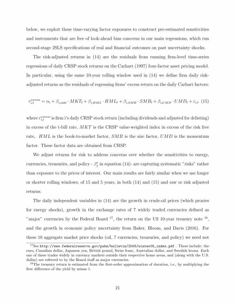
The risk-adjusted returns in (14) are the residuals from running firm-level time-series

regressions of daily CRSP stock returns on the Carhart (1997) four-factor asset pricing model.

In particular, using the same 10-year rolling window used in (14) we define firm daily risk-

adjusted returns as the residuals of regressing firms’ excess return on the daily Carhart factors:

rexcessi,t = αi + βi,mkt ·MKTt + βi,HML ·HMLt + βi,SMB · SMBt + βi,UMD ·UMDt + εi,t (15)

where rexcessi,t is firm i’s daily CRSP stock return (including dividends and adjusted for delisting)

in excess of the t-bill rate, MKT is the CRSP value-weighted index in excess of the risk free

rate, HML is the book-to-market factor, SMB is the size factor, UMD is the momentum

factor. These factor data are obtained from CRSP.

We adjust returns for risk to address concerns over whether the sensitivities to energy,

currencies, treasuries, and policy - βcj in equation (14)- are capturing systematic ”risks” rather

than exposure to the prices of interest. Our main results are fairly similar when we use longer

or shorter rolling windows, of 15 and 5 years, in both (14) and (15) and raw or risk adjusted

returns.

The daily independent variables in (14) are the growth in crude-oil prices (which proxies

for energy shocks), growth in the exchange rates of 7 widely traded currencies defined as

”major” currencies by the Federal Board 17, the return on the US 10-year treasury note 18,

and the growth in economic policy uncertainty from Baker, Bloom, and Davis (2016). For

these 10 aggregate market price shocks (oil, 7 currencies, treasuries, and policy) we need not

17See http://www.federalreserve.gov/pubs/bulletin/2005/winter05_index.pdf . These include: theeuro, Canadian dollar, Japanese yen, British pound, Swiss franc, Australian dollar, and Swedish krona. Eachone of these trades widely in currency markets outside their respective home areas, and (along with the U.S.dollar) are referred to by the Board staff as major currencies.

18The treasury return is estimated from the first-order approximation of duration, i.e., by multiplying thefirst difference of the yield by minus 1.

21

only their daily returns (for calculating the sensitivities βcj in equation (14)) but also their

implied volatilities σct as measures of aggregate sources of uncertainty.

Construction of instruments To instrument for firm-level uncertainty shocks, ∆σi,t,

we also require data on aggregate uncertainty shocks, ∆σct . We define the annual uncertainty

on oil, currency, and 10-year treasuries as the 252-day average of daily implied volatility of

oil and currencies from Bloomberg and for treasuries we use the 252-day average of daily

implied volatility for the 10-year US Treasury Note from the Cboe/CBOT (ticker TYVIX).

Likewise, for annual policy uncertainty we employ the 365-day average of the US economic

policy uncertainty index from Baker, Bloom, and Davis (2016). These 10 annual aggregate

uncertainty measures, σct , are used in constructing cross-industry exposures to aggregate

uncertainty shocks, | βc,weightedj | ·∆σct .

We do this in two steps. First, we adjust the factor sensitivities estimated in (14) for their

statistical significance. In particular, within each industry we construct significance-weighted

sensitivities βc,weightedj = ωcj · βcj, where the first term is a sensitivity weight constructed from

the ratio of the absolute value of the t-statistic of each instrument’s sensitivity to the sum

of all t-statistics in absolute value of instruments within the industry, ωcj =abs(tcj)c∑abs(tcj)

. Thus,

we adjust the sensitivities within each industry by their statistical power in (14). However,

in constructing the weights ωcj we first set to zero each individual t-statistic for which the

corresponding sensitivity is statistically insignificant at the 10% level. This is done both

before taking the absolute value of each t-statistic and the sum of their absolute values. Thus,

the significance-weighted sensitivities βc,weightedj can be zero for certain industries. However,

recalling that the raw sensitivities βcj in (14) are estimated in rolling windows, the significance-

weighted sensitivities βc,weightedj need not be zero at every moment in time. Indeed, our sample

shows that 3-SIC industries fluctuate both in their extensive and intensive exposure to the each

of our 10 instruments over time. Our weighting scheme captures and exploits both margins.

Second, we construct 10 composite terms | βc,weightedj | ·∆σct , which we refer to as the

industry-by-year exposure for uncertainty shocks, where the first term is the absolute value

22

of the significance-weighted sensitivity explained above and ∆σct is the annual growth in the

aggregate implied volatility of the instrument. Thus, our instrumental variables estimation

uses 10 instruments, the oil exposure term, the seven currencies exposure terms, the 10-

year treasury exposure term, and the policy-uncertainty exposure term. These 10 composite

industry-by-year exposure for uncertainty shocks are the instruments used in our 2SLS

regressions that instrument for firm-level uncertainty shocks.

Finally, to disentangle second moment effects from first moment effects of our 10

instruments, we also include as controls in the second stage of the 2SLS regressions the

exposure to the returns of each instrument (i.e., first moment controls). That is, in the

regressions we also include 10 first moment composite terms βc,weightedj · rct .19 Thus, our

empirical examination focuses on the effects of uncertainty shocks above and beyond first

moment effects. At the firm-level, our main set of controls further includes each individual

firms’ measure of first moment effects, i.e., the CRSP stock return of the firm, ri,t (which

accounts for discount rate channel effects).

5 Empirical findings

We start by examining how volatility shocks relate to firm-level capital investment rates,

followed by other real outcomes -intangible capital investment, employment, and cost of goods

sold- and then by financial variables -debt, payout, and cash holdings.

5.1 Investment results

Table 3 examines how uncertainty influences future capital investment rates. Column 1

presents the univariate Ordinary Least Squares regression results of investment rate on lagged

annual realized stock return volatility shocks. We observe highly statistically significant

coefficients (t-stat of 20.075) on return volatility, showing that firms tend to invest more when

19For economic policy uncertainty we measure rct as growth from one year to the next in the 4-quarteraverage of the level of government expenditure as a share of GDP. For currencies, oil, and treasuries returnsrct are the 252-day average of daily returns.

23

their firm-specific uncertainty is low. Column 4 presents the corresponding OLS univariate

regression results of investment rate on lagged firm-level implied volatility shocks (from

OptionMetrics). The sign of the coefficient is consistent with realized volatility shocks, but

the size is more than twice as large, potentially because implied volatility is a better measure

of uncertainty.20

One obvious concern with these OLS regressions is endogeneity - for example, changes in

firms’ investment plans could change stock-prices. Using lagged uncertainty mitigates some

of these concerns, but given stock prices are forward looking movements in returns still suffer

from endogeneity concerns. Therefore. we try to address endogeneity concerns with our

instrumentation strategy. In particular, columns 2 and 3 instrument lagged realized volatility

shocks using the full set of 10 instruments while columns 5 and 6 instrument lagged implied

volatility shocks. Columns 2 and 5 are univariate while 3 and 6 are multivariate with a full set

of controls. In all cases we find that uncertainty shocks lead to significant drops in firm-level

investment.

The point estimates of the coefficients on instrumented uncertainty shocks with the full

set of controls are roughly of comparable magnitude to the univariate OLS point estimates

(e.g., columns 3 and 1). Our full set of lagged controls includes Tobin’s Q, log sales and stock-

returns to control for firm moment shocks, as well as book leverage, profitability (return on

assets) and tangibility to control for financial conditions. Our multivariate specifications also

include firm and time fixed effects and cluster standard errors at the 3-SIC industry (which

is the same level at which our instrumentation strategy estimates factor exposures). In all

instrumented cases, rises in uncertainty is a strong predictor of future reductions in capital

investment rates.

In terms of magnitudes the results imply that a two-standard deviation increase in realized

volatility (see the descriptive statistics in Table A2) would reduce investment by between 4%

to 6% (using the results from our preferred multivariate specifications in column (3) and (6)).

20We reestimate both specifications in columns (1) and (4) on a common sample of 17,391 observations intable (A5) and find the realized and implied volatility coefficients are -0.033 and -0.079.

24

This is moderate in comparison to firm-level investment fluctuations which have a standard

deviation of 24.7%, but is large when considering that annual investment rates drop between

2% to 6% during recessions as show in Figure 1.

5.1.1 First stage results

The first stage instrumental investment results are shown in Table 4. Columns (1) and (2)

report the first stages for the univariate IV columns (2) and (4) from table 3. We see that

the F-statistics indicate a well identified first stage with respective values of 157.6 and 78.37

for the Cragg-Donald (CD) F-Statistics (robust standard-errors), and 18.58 and 14.96 for the

Kleibergen-Paap (KP) F statistic (SIC-3 digit clustering). We also find the Hansen over-

identifying test does not reject the validity of our instruments with p-values of 0.349 and

0.625. As another check of our identification strategy we would like to see that each of our

instruments is individually positively, and generally significantly correlated with uncertainty

shocks. Indeed, we see in columns (1) and (2) that all 10 instruments are positive and mostly

significant in the first stage.

We repeat the above examination but adding our full set of controls, where columns (3)

and (4) in Table 4 present the first stage for the multivariate IV regressions of columns (3)

and (6) from table 3. Even when we add our full set of controls we see a well satisfied

relevance condition, with CD F-statistics of 171.1 and 58.59, and KP F-statistics of 17.57 and

11.14, respectively, and non-rejected Sargan-Hansen validity test p-values of 0.955 and 0.950.

Moreover, each instrument remains individually positively correlated with uncertainty shocks.

5.2 Intangible capital, employment, and cost of goods sold

Table 5 examines the predictive and causal implications of uncertainty shocks on the growth

of other real outcomes. In particular, Panel A examines investment in intangible capital (as

measured by expenditure on general and administration and R&D, which extends the approach

of Eisfeldt and Papanikolaou (2013)), Panel B examines employment, and Panel C examines

25

the cost of goods sold. In each panel we present the same 6 specification results presented

for investment in Table 3. but to preserve space we drop the point coefficient estimates on

controls and keep only the estimates on lagged uncertainty shocks.

The three panels show that realized and implied volatility shocks are negatively related to

future changes in intangible capital investment, employment, and cost of goods sold. As with

investment, these regressions show a strong first-stage with 3-SIC clustering KP F-statistics

in the range of 9.62 to 17.46 in all multivariate specifications that include a full set of controls,

columns (3) and (6). In our preferred specification of column (3), which instruments realized

lagged uncertainty shocks, both intangible capital investment and cost of good sold drop upon

higher realized uncertainty (significant at the 5 and 1 percent, respectively), while the response

of employment is negative but not statistically significant.

Overall, the three panels confirm the robustness of the causal impact of uncertainty shocks

on real firm activity, even in the presence of extensive first-moment and financial condition

controls, plus an extensive instrumentation strategy for uncertainty shocks.

5.3 Financial variables

Table 6 examines how firm uncertainty shocks affect future changes in financial variables.

In particular, Panel A examines total debt, Panel B dividend payout, and Panel C cash

holdings. Panel A indicates that increases in uncertainty reduce the willingness of firm’s to

increases their overall debt. The correlations are strong and significant in both the OLS and

instrumental variable regressions. Panel B indicates that firm’s take a more cautious financial

approach toward corporate payout. Consistent with a precautionary savings motive, rises in

firm uncertainty causes a large reduction in cash dividend payout. Similarly, Panel C further

evidences a precautionary savings channel as cash holdings increase upon large uncertainty

shocks. In particular, firms accumulate cash reserves and short-term liquid instruments

following uncertainty rises.

For the preferred specifications in columns (3) and (6) all three panel show highly significant

26

point estimates (at the 5% and 1%), strong first stage F-statistics (all KP F-statistics above

11.1), and non-rejections on the Sargan-Hansen over-identifying test. This highlights that our

instrumental strategy based on exchange rate and factor price volatility works well not only

for real outcomes but also for financial.

5.4 Instrument and credit supply robustness

In Appendix Table A3 we investigate the main multivariate investment results dropping each

instrument one-by-one in columns (2) to (9) to show our results are not being driven by

any particular instrument (noting in column (10) we drop the oil and treasury instruments

together to allow us to extend our sample size to 42,388)21. As we see across the columns the

first stage results for investment are impressively robust - the tougher KP F-test test is in

the range of 12.09 to 19.84 in all specifications (the CD F–test is always above 99), and the

Hansen over-identifying test does not reject in any specification with p-values of 0.9 or above.

Moreover, all real and financial variables examined in baseline column (1) are robust. Taken

together, the results across all columns indicate that our identification results are not driven

by one particular instrument, but instead are driven by the combined identification of energy,

exchange rate, policy, and treasury uncertainty driving firm-level uncertainty fluctuations and

firm decisions. This suggests that our identification strategy will likely be broadly useful for

a wide-range of models of the causal impact of uncertainty on firm behavior.

In Appendix Table A4 we investigate the robustness of the results to both adjusting

volatility shocks by firm leverage and including controls for financial constraints. In columns

(1) and (1A) we regress all main real and financial outcomes on lagged leverage-adjusted

realized and implied volatility shocks, respectively. Here we adjust uncertainty effects by

multiplying either volatility by firm’s book leverage, i.e., σi,t · Ei,t

Ei,t+Di,twhere E is book equity

(CEQ in Compustat) and D is total debt. The results are robust to these levered-volatility

measures. Moreover, one concern could be that uncertainty reduces financial supply - for

21Oil and 10-year treasury daily implied volatility data starts in March 2003, whereas implied volatility dataon the Euro-USD bilateral exchange rate starts in 1999 and policy in 1985.

27

example, banks are unwilling to lend in periods of high uncertainty - which causes the results

we observe. To try to address this we include a variety of different controls for firms financial

conditions and show our baseline results are robust to this. In particular for both the realized

and implied volatility specifications we include controls for firm: CAPM-beta (defined as the

covariance of the firms daily returns with the market returns in the past year, scaled by the

variance of the market) in columns 2 and 2A, a broad set of firm financial constraint controls

in columns 3 and 3A - which include the lags for the Whited and Wu (2006) index, size and age

(SA) index of Hadlock and Pierce (2010), the Kaplan and Zingales (1997) index, reciprocal of

total assets, reciprocal of employees, and reciprocal of age -where age is the number of years

since firm incorporation-, the firms long-term credit rating from S&P in columns 4 and 4A

(which consist of a full set of dummies based on every possible credit rating category given

to firms by S&P on long-term debt, where the omitted dummy is for no credit ratings), and

all of the previous measures combined in columns 5 and 5A. In summary, as we can see from

Table A4 including these financial supply variables does not notably change our results. So

while these are not perfect controls for financial conditions, the robustness of our results to

their inclusion helps address concerns that financial supply conditions are the main driver of

our results.

In Appendix Table A5 we re-examine our main investment Table 3 but holding the sample

of firm-time observations to be the same across specifications (1) to (6). In particular, our

sample is constrained by the availability of OptionMetrics data on firm-level implied volatility,

which gives a total of 17,391 observations across all columns. Compared to the main Table 3

the point estimates on the coefficients are largely comparable in both magnitude and statistical

significance. Therefore, differences in point estimates across specifications (2SLS vs OLS,

univariate vs multivariate, and realized vs implied volatility shocks) are primarily due to the

underlying specifications themselves and not due to differences in sample size.

Finally, in Appendix Table A6 we further present dividend payout results when defined as

a ratio of lagged total assets (Payouti,tATi,t−1

). The causal effects of uncertainty shocks are robust to

28

using this alternative definition of dividend payout, which complements the dividend growth

results presented in Panel B of Table 6.

5.5 The finance uncertainty multiplier

Finally, Table 7 shows the results from running a series of finance-uncertainty interactions

on the data during the core Jan. 2008-Dec. 2009 period of the financial crisis. By running

double and triple interaction of uncertainty with financing frictions we attempt to tease out the

finance-uncertainty multiplier effects examined in the model of section 2. In particular, Table

7 examines the impact of realized volatility shocks on investment for financially constrained

and unconstrained firms during financial crisis and non-crisis years. We do this by running

the following specification and subsets of it:

Ii,t/Ki,t−1 = β0 + β1∆σi,t−1 + β2Dcrisis year,t

+β3Dcrisis year,t ·∆σi,t−1 + β4Dfin.constrained,i,t−1 + β5Dfin.constrained,i,t−1 ·∆σi,t−1

+β6Dcrisis year,t ·Dfin.constrained,i,t−1 + β7Dcrisis year,t ·Dfin.constrained,i,t−1 ·∆σi,t−1 (16)

where ∆σi,t−1is firm i′s growth of realized annual vol from year t − 2 to t − 1, Dcrisis year,t is

a dummy that takes value of 1 for all firm fiscal-year observations of investment rate ending

in calendar years 2008 and 2009, i.e., core years of the financial crisis which comprise the

core months of the great recession in which firms would have observed at least 6 months

of heightened financial frictions in their annual accounting reports, zero otherwise, and

Dfin.constrained,i,t−1is a dummy that takes value of 1 for firms classified as financially constrained

(e.g., according to Whited-Wu index) in year t−1, zero otherwise. The coefficient β7 indicates

whether the effect of uncertainty on investment is different for financially constrained firms

during crisis years relative to unconstrained firms.22

22There is a large literature on measuring firm-level financial constraints. Any proxies are usually subjectto critiques on whether they truly capture constraints or just noise. We employ a total of 6 different proxiesto take rough cuts to our Compustat data. We thank Toni Whited for suggestions on this front, e.g., addingthe SA index.

29

Column (1) presents our baseline 2SLS multivariate specification with full set of controls

presented in Table 3 column (3). Column (2) interacts past uncertainty shocks with the

contemporaneous crisis dummy, Dcrisis year,t. The regression indicates that the effects of

uncertainty shocks on investment are much larger in the period of high financing frictions

in the core crisis years of the great recession, as seen in the highly significant interaction

term Dcrisis year,t ·∆σi,t−1. This is consistent with the main thesis in this paper that financial

constraints substantially amplify the impact of uncertainty shocks.

To disentangle and further understand these financing frictions vs uncertainty effects,

columns (3) to (8) run the full difference-in-difference-in-difference specification in 16 , where

we employ a total of 6 proxies for financing frictions to classify firms into financially constrained

and unconstrained groups. For example, in column (4) using each firm’s financial constraint

Whited-Wu index at every fiscal year t−1 we classify firms into constrained and unconstrained

groups using the 40 and 60 percentile cutoffs obtained from the cross-sectional fiscal-year

distribution of the given index. We consider a firm constrained if its t− 1 index value is equal

to or greater than the 60 percentile and unconstrained if equal to or less than the 40 percentile.

We exclude firm-time observations in the middle 50+/-10 percentiles to increase precision in

the classification of firms.23 We do this in all but the S&P credit-rating financial constraint

measure, column (3). Here we follow Duchin, Ozbas, and Sensoy (2010) and consider a firm

constrained if it has positive debt and no bond rating and unconstrained otherwise (which

includes firms with zero debt and no debt rating).24

In sum the 6 measures of financial constraints are constructed using S&P ratings column

(3), Whited-Wu index column (4), reciprocal of employees column (5), reciprocal of total

assets column (6), reciprocal of age column (7) in which age is defined as the number of

years since firm incorporation, and the SA index based on size and age of Hadlock and Pierce

23Our inferences are similar if we expand or reduce the window of observations dropped in the middle: 50+/-15 and/or 50+/-5 percentiles, i.e., comparing top vs bottom 30% and/or 45% of firms. Moreover, results aresimilar if we classify firms as ex-ante financially constrained or unconstrained using two-year past indexes offinancial constraints.

24For ratings data we use Compustat-Capital IQ’s ratings data from WRDS, where ratings dummies arebased on variable SPLTICRM (S&P Domestic Long-Term Issuer Credit Rating).

30

(2010) column (8). In all specifications we include both firm and calendar-year fixed effects,

and cluster standard errors at the 3 digit SIC industry. All specifications include full set of

controls of baseline specification column (1).

Using the Whited-Wu index column (4) to classify firms, the results indicate that

investment rates drop upon larger uncertainty shocks (negative and significant β1 coefficient

on uncertainty shock ∆σi,t−1, at the 5%), the drop is more pronounced during the core crisis

years of 2008 and 2009 (negative and significant β3 coefficient on the double interaction term

Dcrisis year,t ·∆σi,t−1, at the 1%), and the negative real effect on investment is amplified for ex-

ante financially constrained firms during the core crisis years (as determined by the negative

and significant β7 coefficient on the triple interaction term Dcrisis year,t · Dfin.constrained,i,t−1 ·

∆σi,t−1, at the 5%).

Using other measures of financial constraints in columns (3) to (8) give similar inferences:

uncertainty matters (causally), it matters even more during periods of financial constraints,

and it matters most for the most ex-ante constrained firms. Hence, overall Table 7 provides

important empirical evidence in support of the testable predictions of the model of section 2

for an interactive effect of financial constraints and uncertainty in deterring firm investment

activities during the 2008-2009 period of the financial crisis.

To show this graphically in the raw data Figure 7 plots investment rates for financially

constrained and unconstrained firms from 2003 to 2013. We normalize the investment rates

of both groups of firms to their respective values of investment rates in 2006. Financial

constraints are defined as a firm having short or long-term debt but no public bond rating

(see, e.g., Faulkender and Petersen (2006) and Duchin, Ozbas, and Sensoy (2010)). Volatility is

the annual realized stock return volatility of all firms in the sample. It is clear that constrained

and unconstrained firms’ investment rates track each other closely until the Great Recession,

at which point the constrained firms’ investment drop substantially more than unconstrained

firms. As uncertainty recedes post 2012 the gaps start to recede again as the investment rates

begin to converge. There are of course many ways to explain this difference (e.g. small vs

31

large firms), but it is at least consistent with the model of uncertainty shocks mattering more

for more financially constrained firms.

As a robustness Appendix Table A7 repeats the examination done in Table 7, but using

option-implied firm-level uncertainty shocks instead of realized uncertainty shocks. The

inferences on the economic and financial importance of uncertainty shocks are robust to these

forward-looking uncertainty data.

6 Conclusion

This paper studies the impact of uncertainty shocks on firms’ real and financial activity both

theoretically and empirically. We build a dynamic model which adds two key components:

first, real and financial frictions, and second, uncertainty and financial shocks. This delivers

three key insights. First, combining real and financial frictions roughly doubles the impact

of uncertainty shocks - this is the finance uncertainty multiplier. Second, combining an

uncertainty shock with a financial shock in this model increases the impact by about another

two thirds, since these shocks have an almost additive effect. Since uncertainty and financial

shocks are highly collinear (e.g. Stock and Watson 2012) this is important for modelling their

impacts. Finally, in this model uncertainty shocks not only reduce investment and hiring, but

also raise firms cash holding, while cutting equity payouts. Collectively, these predictions of a

large impact of uncertainty shocks on real and financial variables matches the evidence from

the recent financial crisis.

We then use empirical data on U.S. listed firms to test the model using a novel

instrumentation strategy. Consistent with the testable implications, uncertainty shocks reduce

firm investment (tangible and intangible) and employment on the real side, and increase cash

holdings, while reducing payouts and debt on the financial side.

In all, our theoretical and empirical analyses show that real and financial frictions are

quantitatively crucial to explain the full impact of uncertainty shocks on real and financial

activity.

32

References

Abel, A., and J. Eberly (1996): “Optimal Investment With Costly Reversibility,” Reviewof Economic Studies, 63, 581–593.

Alessandri, P., and H. Mumtaz (2016): “Financial regimes and uncertainty shocks,”QMW mimeo.

Altinkilic, O., and R. S. Hansen (2000): “Are There Economies of Scale in UnderwritingFees? Evidence of Rising External Financing Costs,” Review of Financial Studies, 13, 191–218.

Arellano, C., Y. Bai, and P. J. Kehoe (2016): “Financial Frictions and Fluctuationsin Volatility,” Working Paper.

Asquith, P., and D. Mullins (1986): “Equity issues and offering dilution,” Journal ofFinancial Economics, 15, 61–89.

Bachmann, R., and C. Bayer (2013): “Wait-and-See Business Cycles?,” Journal ofMonetary Economics, 60(6), 704–719.

Bachmann, R., and G. Moscarini (2012): “Business Cycles and EndogenousUncertainty,” Working Paper, University of Notre Dame and Yale University.

Baker, S., N. Bloom, and S. Davis (2016): “Measuring Economic Policy Uncertainty,”Forthcoming Quarterly Journal of Economics.

Bansal, R., and A. Yaron (2004): “Risks for the long run: A potential resolution of assetpricing puzzles.,” Journal of Finance, 59, 1481–1509.

Barro, R. (2006): “Rare disasters and asset markets in the twentieth century,” QuarterlyJournal of Economics, 121(3), 823–866.

Basu, S., and B. Bundick (2017): “Uncertainty Shocks in a Model of Effective Demand,”NBER Working Paper No. 18420.

Berger, D., I. Dew-Becker, and S. Giglio (2016): “Contractionary volatility or volatilecontractions?,” Working paper, Northwestern University.

Bernanke, B., and M. Gertler (1989): “Agency costs, net worth, and businessfluctuations,” American Economic Review, 79(1), 14–31.

Bernanke, B. S. (1983): “Irreversibility, Uncertainty, and Cyclical Investment,” QuarterlyJournal of Economics, 98(1), 85–106.

Bertola, G., and R. J. Caballero (1990): “Kinked Adjustment Costs and AggregateDynamics,” NBER Macroeconomics Annual, 5, 237–296.

Bigio, S. (2015): “Endogenous liquidity and the business cycle,” American Economic Review,105(6), 1883–1927.

Bloom, N. (2009): “The Impact of Uncertainty Shocks,” Econometrica, 77, 623–685.Bloom, N., M. Floetotto, N. Jaimovich, I. Saporta-Eksten, and S. Terry

(2016): “Really uncertain business cycles,” National Bureau of Economic Research, StanfordUniversity.

Bolton, P., H. Chen, and N. Wang (2011): “A unified theory of Tobin’s q, corporateinvestment, financing, and risk management,” Journal of Finance, 66, 1545–1578.

Bolton, P., H. Chen, and N. Wang (2013): “Market timing, investmentand riskmanagement,” Journal of Financial Economics, 109, 40–62.

Caballero, R., E. Engel, and J. Haltiwanger (1995): “Plant-level adjustment andaggregate investment dynamics,” Brookings Papers on Economic Activity, 2, 1–54.

33

Carhart, M. (1997): “On Persistence in Mutual Fund Performance,” Journal of Finance,52,1, 57–82.

Carlstrom, C. T., and T. S. Fuerst (1997): “Agency costs, net worth, and businessfluctuations: A computable general equilibrium analysis,” American Economic Review,87(5), 893–910.

Chen, G. (2016): “Corporate Savings, Financingand Investment with Aggregate UncertaintyShocks,” Working Paper, Nanyang Technological University.

Chen, H., H. Wang, and H. Zhou (2014): “Stock Return Volatility and Capital StructureDecisions,” PBCSF-NIFR, Tsinghua University, 13,04.

Choe, H., R. Masulis, , and V. Nanda (1993): “Common Stock Offerings across theBusiness Cycle: Theory and Evidence,” Journal of Empirical Finance, 1, 3–31.

Christiano, L. J., R. Motto, and M. Rostagno (2014): “Risk Shocks,” AmericanEconomic Review, 104, 27–65.

Cooley, T. F., and V. Quadrini (2001): “Financial markets and firm dynamics,”American Economic Review, 91, 1286–1310.

Cooper, R., and J. Haltiwanger (2006): “On the nature of capital adjustment costs,”Review of Economic Studies, 73, 611–633.

Davis, S. J., and J. Haltiwanger (1992): “Gross Job Creation, Gross Job Destruction,and Employment Reallocation,” The Quarterly Journal of Economics, MIT Press, 107,3,819–863.

DeAngelo, H., L. DeAngelo, and T. M. Whited (2011): “Capital structure dynamicsand transitory debt,” Journal of Financial Economics, 99, 235–261.

Dixit, A. K., and R. S. Pindyck (1994): Investment under Uncertainty. Princeton:Princeton University Press, Princeton, N.J.

Duchin, R., O. Ozbas, and B. Sensoy (2010): “Costly external finance, corporateinvestmentand the subprime mortgage credit crisis,” Journal of Financial Economics, 97,418–435.

Eisfeldt, A. (2004): “Endogenous liquidity in asset markets,” Journal of Finance, 59(1),1–30.

Eisfeldt, A., and T. Muir (2016): “Aggregate External Financing and Savings Waves,”Journal of Monetary Economics, 84, 116–133.

Erel, I., B. Julio, W. Kim, and M. Weisbach (2012): “Macroeconomic Conditions andCapital Raising,” Review of Financial Studies, 25, 341–376.

Falgelbaum, P., E. Schaal, and M. Taschereau-Dumouchel (2016): “UncertaintyTraps,” Forthcoming, Quarterly Journal of Economics.

Faulkender, M., and M. Petersen (2006): “Does the source of capital affect capitalstructure?,” Review of Financial Studies, 19, 45–79.

Fernandez-Villaverde, J., P. Guerron-Quintana, K. Kuester, and J. Rubio-Ramirez (2015): “Fiscal Volatility Shocks and Economic Activity,” American EconomicReview, 105(11), 33523384.

Fernandez-Villaverde, J., P. G. Quintana, J. F. Rubio-Ramirez, and M. Uribe(2011): “Risk Matters: The Real Effects of Volatility Shocks,” American Economic Review,101,6, 2530–61.

Gilchrist, S., J. Sim, and E. Zakrajsek (2014): “Uncertainty, Financial Frictions andInvestment Dynamics,” Boston University mimeo.

34

Gomes, J. (2001): “Financing investment,” American Economic Review, 65(2), 467–494.Gourio, F. (2012): “Disaster Risk and Business Cycles,” American Economic Review,

102(6), 2734–2766.Graham, J. (2000): “How big are the tax benefits of debt?,” Journal of Finance, 55(5),

1901–1941.Guiso, L., and G. Parigi (1999): “Investment and Demand Uncertainty,” Quarterly Journal

of Economics, 114, 185–227.Hadlock, C. J., and J. R. Pierce (2010): “New Evidence on Measuring Financial

Constraints: Moving Beyond the KZ Index,” The Review of Financial Studies, 23(5), 1909–1940.

Handley, K., and N. Limao (2012): “Trade and Investment under Policy Uncertainty:Theory and Firm Evidence,” NBER Working Paper 17790.

Hennessy, C. A., A. Levy, and T. M. Whited (2007): “Testing Q theory with financingfrictions,” Journal of Financial Economics, 83(3), 691–717.

Hennessy, C. A., and T. M. Whited (2005): “Debt Dynamics,” Journal of Finance, 60,1129–1165.

(2007): “How costly is external financing? Evidence from a structural estimation,”Journal of Finance, 62, 1705–1745.

Ilut, C., and M. Schneider (2014): “Ambiguous Business Cycles,” American EconomicReview, 104(8), 2368–99.

Jermann, U., and V. Quadrini (2012): “Macroeconomic Effects of Financial Shocks,”American Economic Review, 102(1), 238–71.

Kahle, K., and R. Stulz (2013): “Access to Capital, Investment, and the Financial Crisis,”Journal of Financial Economics, 110(2), 280–299.

Kaplan, S., and L. Zingales (1997): “Do investment cash-flow sensitivities provide usefulmeasures of financing constraints?,” Quarterly Journal of Economics, 112, 169–215.

Khan, A., and J. Thomas (2008): “Idiosyncratic Shocks and the Role of Nonconvexitiesin Plant and Aggregate Investment Dynamics,” Econometrica, 76,2, 395–436.

Khan, A., and J. K. Thomas (2013): “Credit shocks and aggregate fluctuations in aneconomy with production heterogeneity,” The Review of Financial Studies, 121(6), 1055–1107.

King, R., and S. Rebelo (1999): Handbook of Macroeconomics. North-Holland,Amsterdam, Netherlands, Resuscitating real business cycles.

Krusell, P., and A. A. Smith (1998): “Income and Wealth Heterogeneity in theMacroeconomy,” Journal of Political Economy, 106(5), 867–896.

Kurlat, P. (2013): “Lemons markets and the transmission of aggregate shocks,” AmericanEconomic Review, 103(4), 1463–1489.

Leahy, J. V., and T. Whited (1996): “The Effect of Uncertainty on Investment: SomeStylized Facts,” Journal of Money, Creditand Banking, 28, 64–83.

Leary, M. T., and M. R. Roberts (2014): “Do Peer Firms Affect Corporate FinancialPolicy?,” Journal of Finance, 69(1), 139–178.

Lee, G., and R. W. Masulis (2009): “Seasoned equity offerings: Quality of accountinginformation and expected flotation costs,” Journal of Financial Economics, 92(3), 443–469.

Lhuissier, S., and F. Tripier (2016): “Do uncertainty shocks always matter for businesscycles?,” CEPII working paper.

35

Moyen, N. (2004): “Investment-cash flow sensitivities: Constrained versus unconstrainedfirms,” Journal of Finance, 59, 2061–2092.

Nieuwerburgh, S. V., and L. Veldkamp (2006): “Learning Asymmetries in RealBusiness Cycles,” Journal of Monetary Economics, 53, 753–772.

Orlik, A., and L. Veldkamp (2015): “Understanding Uncertainty Shocks and the Role ofthe Black Swan,” Working paper, NYU.

Pastor, L., and R. Stambaugh (2003): “Liquidity Risk and Expected Stock Returns,”Journal of Political Economy, 111, 642–685.

Pastor, L., and P. Veronesi (2012): “Uncertainty about Government Policy and StockPrices,” Journal of Finance, 67, 1219–1264.

Rajan, R. G., and L. Zingales (1995): “What do we know about capital structure? Someevidence from international data,” Journal of Finance, 50, 1421–1460.

Ramey, V., and G. Ramey (1995): “Cross-country evidence on the link between volatilityand growth,” American Economic Review, 85,5, 1138–51.

Rampini, A., and S. Viswanathan (2013): “Collateral and capital structure,” Journal ofFinancial Economics, 109, 466–492.

Riddick, L. A., and T. M. Whited (2009): “The corporate propensity to save,” Journalof Finance, 64, 1729–1766.

Rietz, T. (1988): “The equity premium: a solution,” Journal of Monetary Economics, 22(1),117131.

Romer, C. (1990): “The Great Crash and the Onset of the Great Depression,” QuarterlyJournal of Economics, 105(3), 597–624.

Segal, G., I. Shaliastovich, and A. Yaron (2015): “Good and Bad Uncertainty:Macroeconomic and Financial Market Implications,” Journal of Financial Economics, 117,369–397.

Stein, L., and E. Stone (2013): “The effect of uncertainty on investment, hiring and RD:causal evidence from equity options,” Arizona State University mimeo.

Stock, J., and M. Watson (2012): “Disentangling the channels of the 2007-09 recession,”Brookings Papers on Economic Activity, 1, 81–135.

Welch, I. (2004): “Capital Structure and Stock Returns,” Journal of Political Economy,112, 106–131.

Whited, T., and G. Wu (2006): “Financial constraints risk,” Review of Financial Studies,19, 531–559.

36

Table

1P

ara

mete

rvalu

es

under

bench

mark

calibra

tion

Desc

rip

tion

Nota

tion

Valu

eJu

stifi

cati

on

Tech

nolo

gy

Su

bje

ctiv

ed

isco

unt

fact

or

β0.

988

Lon

g-ru

nav

erag

eof

U.S

.fi

rm-l

evel

dis

cou

nt

rate

Ret

urn

onsa

vin

gr n

0.01

80%

ofth

eri

sk-f

ree

rate

(th

eca

shto

asse

tra

tio

for

cash

hold

ing

firm

s)

Sh

are

onca

pit

alα

0.33

Cap

ital

shar

ein

outp

ut

ison

e-th

ird

,la

bor

shar

eis

two-

thir

ds

Mar

ku

pε

433

%m

arku

p.

Wit

hco

nst

ant

retu

rns

tosc

ale

yie

lds

a+

b=

0.7

5

Wag

ew

1W

age

rate

nor

mal

ized

to1

Rat

eof

dep

reci

atio

nfo

rca

pit

alδ

0.03

Cap

ital

dep

reci

atio

nra

teas

sum

ed3%

per

qu

arte

r

Fix

edco

stof

inve

stm

ent

c k0.

011%

ofqu

arte

rly

reve

nu

e(A

lso

trie

d2%

&4%

)

Fix

edop

erat

ing

cost

F0.

2F

irm

s’av

erag

eS

G&

Ato

sale

sra

tio

Un

cert

ain

tysh

ock

(2st

ate

Mark

ov)

Con

dit

ion

alvo

lati

lity

ofp

rod

uct

ivit

yσL

0.05

1B

asel

ine

un

cert

ainty

(Blo

omet

al20

16)

Con

dit

ion

alvo

lati

lity

inh

igh

un

cert

ainty

state

σH

0.20

9U

nce

rtai

nty

shock

s4.

1*b

asel

ine

un

cert

ainty

(Blo

omet

al

2016)

Tra

nsi

tion

pro

bab

ilit

ylo

wto

hig

hu

nce

rtai

nty

πσ L,H

2.60

%U

nce

rtai

nty

shock

sex

pec

ted

ever

y9.

6ye

ars

(Blo

omet

al

2016)

Tra

nsi

tion

pro

bab

ilit

yre

main

ing

inh

igh

un

cert

ainty

πσ H,H

94%

Qu

arte

rly

pro

bab

ilit

yof

rem

ain

ing

inh

igh

un

cert

ainty

(Blo

om

etal

2016)

Per

sist

ence

oflo

gge

did

iosy

ncr

atic

pro

du

ctiv

ity

ρz

0.95

Qu

arte

rly

per

sist

ence

ofid

iosy

ncr

atic

pro

du

ctiv

ity

(Kh

an

&T

hom

as

2008)

Sto

chast

icfi

nan

cin

gcost

(2st

ate

Mark

ov)

Low

exte

rnal

fin

anci

ng

cost

stat

eηL

0.00

5L

owco

st.5

%of

outp

ut

(Alt

inkil

ican

dH

anse

n20

00)

Hig

hex

tern

alfi

nan

cin

gco

stst

ate

ηH

0.05

Hig

hco

st5%

ofou

tpu

t(A

ltin

kil

ic&

Han

sen

2000

).R

ob

ust

2.5

%,1

0%

Tra

nsi

tion

pro

bab

ilit

ylo

wto

hig

hfi

nan

cin

gco

stst

ate

πη L,H

2.60

%S

ame

asu

nce

rtai

nty

shock

(Als

otr

ied

5%)

Tra

nsi

tion

pro

b.

rem

ain

ing

inh

igh

fin

anci

ng

cost

stat

eπη H,H

94%

Sam

eas

un

cert

ainty

shock

(Als

otr

ied

50%

)

Imp

act

ofu

nce

rtai

nty

onfi

nan

cial

cost

λ0.

04C

orre

lati

onb

etw

een

the

Baa

-Aaa

spre

adan

dV

IX

Th

ista

ble

pre

sents

the

pre

det

erm

ined

and

the

calib

rate

dp

aram

eter

valu

esof

the

ben

chm

ark

mod

el.

37

Table 2Coefficient on changes in volatility for real and financial variables

Real Financial

I/K ∆Emp ∆Cash Div/K

A: Data

∆Volatility -0.089 -0.074 0.227 -0.019

B: Real frictions

∆Volatility -0.042 -0.014 na -0.007

C: Financial frictions

∆Volatility -0.021 -0.004 1.032 -0.036

D: Real+financial frictions

∆Volatility -0.080 -0.028 0.487 -0.012

E: No frictions

∆Volatility 0.003 0.006 na -0.021

Row (A) Data reports the results for investment rate, employment growth, cash growth, and equity payoutto assets ratio from columns (2) of tables (3), (5), (6), (A6) respectively. Rows (B) to (E) reports the modelcounterparts from regressions using simulation data on volatility (σi,t) growth. The reported statistics in themodel are from simulated data with 3000 firms and 200 quarterly observations. I/K is the investment rate,∆Emp is the employment growth, ∆Cash is the cash growth rate, and Div/K the dividend scaled by capitalin the model and cash dividend plus repurchase scaled by total assets in the data. For comparability all theregressions (in the data and model) include firm and time fixed effects and all are significant at the 1% levelwith firm-clustered standard errors. The only difference is employment is annual in the real data (since noquarterly real employment data is available).

38

Table 3Investment rate

(1) (2) (3) (4) (5) (6)

Investment ratei,t OLS IV IV OLS IV IV

Realized Realized Realized Implied Implied Implied

∆Volatilityi,t−1 -0.032*** -0.089*** -0.030*** -0.090*** -0.225*** -0.078**

(-20.075) (-3.923) (-2.948) (-10.449) (-4.235) (-2.454)

Book Leveragei,t−1 -0.050*** -0.037***

(-8.173) (-5.583)

Stock Returni,t−1 0.008*** 0.005*

(2.953) (1.808)

Log Salesi,t−1 -0.023*** -0.022***

(-7.330) (-5.290)

Return on Assetsi,t−1 0.142*** 0.132***

(5.558) (3.910)

Tangibilityi,t−1 -0.115*** -0.123***

(-5.801) (-3.355)

Tobin’s Qi,t−1 0.049*** 0.054***

(9.892) (8.341)

1st moment 10IVi,t−1 No No Yes No No Yes

Firm, time FE Yes Yes Yes Yes Yes Yes

SE cluster(3SIC) Yes Yes Yes Yes Yes Yes

Observations 124,206 28,419 28,132 26,030 17,572 17,391

F 1st st. Cragg-D 157.6 171.1 78.37 58.59

F 1st st. Kleib.-P 18.58 17.57 14.96 11.14

p-val Sargan–H J 0.349 0.955 0.625 0.950

Table presents OLS and 2SLS annual regression results of firm-level investment rate on 1-year lagged changesin firm-level volatility and lagged level of firm-level controls. Investment rate at fiscal year t is defined asIt/Kt−1 (capx/lagged net property plant & equipment from Compustat). Sample period is from 1963 to2016. Specifications 1,2,4, and 5 are univariate, while 3 and 6 multivariate. Only 1 and 4 are OLS while allothers 2SLS. The latter instrument lagged changes in firm-level volatility with industry-level (3SIC) exposureto 10 aggregate lagged uncertainty shocks. These include the lagged exposure to annual changes in expectedvolatility of energy, currencies, and 10-year treasuries (as proxied by at-the-money forward-looking impliedvolatilities of oil, 7 widely traded currencies, and TYVIX) and economic policy uncertainty from Baker, Bloom,and Davis (2016). Annual realized volatility is the 12-month standard deviation of daily stock returns fromCRSP. Implied volatility is the annual average of daily (365-day) implied volatility of at-the-money-forwardcall options from OptionMetrics. Regressors lagged by 1-year. Both firm and calendar-year fixed effects areincluded. Standard errors are clustered at the 3-digit SIC industry. To tease out the impact of 2nd momentuncertainty shocks we also include as controls the lagged exposure to changes in the return on each of the 10aggregate instruments (i.e., 1st moment shocks). Data availability on implied volatility of treasuries and oilrestrict the start of the 2SLS sample to fiscal year 2006. Statistical significance: *** p<0.01, ** p<0.05, *p<0.1, † p<0.15. t-statistics are in parentheses. See section 4 for data details.

39

Table 4Investment rate - 2SLS 1st stage results

Specification: Univariate Multivariate

Set-up: ∆Volatilityi,t−1 Realized Implied Realized Implied

∆Vol Exposure Cadi,t−1 3.643*** 1.442*** 3.353*** 1.234***

(4.64) (3.66) (4.54) (3.35)

∆Vol Exposure Euroi,t−1 1.338*** 0.643*** 1.211*** 0.479***

(4.34) (3.57) (4.13) (2.80)

∆Vol Exposure Jpyi,t−1 2.117*** 0.244 2.096*** 0.298

(3.53) (0.55) (3.55) (0.68)

∆Vol Exposure Audi,t−1 5.142*** 1.769*** 5.395*** 1.763***

(7.44) (5.64) (8.90) (5.72)

∆Vol Exposure Seki,t−1 4.236*** 1.277*** 4.914*** 1.575***

(7.56) (3.57) (7.73) (4.10)

∆Vol Exposure Chfi,t−1 2.046*** 1.300*** 2.319*** 1.360***

(5.75) (6.10) (5.90) (5.44)

∆Vol Exposure Gbpi,t−1 2.971*** 1.841*** 2.697*** 1.655***

(5.05) (4.24) (5.05) (4.51)

∆Vol Exposure Policyi,t−1 588.990*** 239.159* 616.792*** 195.837*

(3.02) (1.94) (3.32) (1.72)

∆Vol Expos.Treasuryi,t−1‡ 3.116*** 1.100*** 2.969*** 0.811***

(8.43) (4.45) (8.31) (4.10)

∆Vol Exposure Oili,t−1 3.132*** 1.938*** 4.549*** 1.796***

(9.79) (10.33) (5.90) (6.06)

Observations 28,419 17,572 28,132 17,391

F-test 1st stage Cragg-Donald 157.6 78.37 171.1 58.59

F-test 1st stage Kleibergen-Paap 18.58 14.96 17.57 11.14

p-value Hansen-Sargan J 0.349 0.625 0.955 0.950

Table presents the 2SLS first stage regression results of firm-level investment rate on 1-year lagged changes infirm-level volatility and lagged level of firm-level controls. Columns 1 and 2 are the first stage results for theunivariate specifications (2) and (5) in Table 3, while columns 3 and 4 are the multivariate first stage resultsof specifications (3) and (6). We instrument lagged changes in firm-level volatility with industry-level (3SIC)exposure to 10 aggregate lagged uncertainty shocks. These include the lagged exposure to annual changes inexpected volatility of energy, currencies, and 10-year treasuries (as proxied by at-the-money forward-lookingimplied volatilities of oil, 7 widely traded currencies, and TYVIX) and economic policy uncertainty fromBaker, Bloom, and Davis (2016). Annual realized volatility is the 12-month standard deviation of daily stockreturns from CRSP. Implied volatility is the annual average of daily (365-day) implied volatility of at-the-money-forward call options from OptionMetrics. Regressors lagged by 1-year. Both firm and calendar-yearfixed effects are included. Standard errors are clustered at the 3-digit SIC industry. To tease out the impactof 2nd moment uncertainty shocks we also include as controls the lagged exposure to changes in the returnon each of the 10 aggregate instruments (i.e., 1st moment shocks). Data availability on implied volatility oftreasuries and oil restrict the start of the 2SLS sample to fiscal year 2006. ‡ :The coefficients on treasuries arescaled upward by a factor of 1000 for presentational purposes. Statistical significance: *** p<0.01, ** p<0.05,* p<0.1, † p<0.15. t-statistics are in parentheses. See section 4 for data details.

40

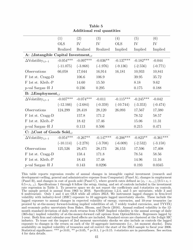
Table 5Additional real quantities

(1) (2) (3) (4) (5) (6)

OLS IV IV OLS IV IV

Realized Realized Realized Implied Implied Implied

A: ∆Intangible Capital Investmenti,t

∆Volatilityi,t−1 -0.054*** -0.097*** -0.036** -0.137*** -0.182*** -0.044

(-11.075) (-3.868) (-1.976) (-9.136) (-2.556) (-0.771)

Observations 66,058 17,044 16,914 16,181 10,933 10,841

F 1st st. Cragg-D 106.6 106.9 39.95 35.72

F 1st st. Kleib.-P 14.60 15.50 8.18 9.62

p-val Sargan–H J 0.236 0.295 0.175 0.188

B: ∆Employmenti,t

∆Volatilityi,t−1 -0.037*** -0.074*** -0.011 -0.115*** -0.245*** -0.042

(-12.166) (-2.684) (-0.359) (-10.744) (-3.353) (-0.474)

Observations 124,299 28,418 28,120 26,093 17,567 17,380

F 1st st. Cragg-D 157.8 171.2 78.52 58.57

F 1st st. Kleib.-P 18.42 17.46 15.06 11.31

p-val Sargan–H J 0.113 0.506 0.215 0.471

C: ∆Cost of Goods Soldi,t

∆Volatilityi,t−1 -0.054*** -0.267** -0.147*** -0.206*** -0.823** -0.361***

(-10.114) (-2.278) (-3.708) (-6.009) (-2.532) (-3.158)

Observations 125,526 28,471 28,173 26,153 17,596 17,408

F 1st st. Cragg-D 158.4 171.8 78.54 58.56

F 1st st. Kleib.-P 18.43 17.48 14.96 11.16

p-val Sargan–H J 0.143 0.0296 0.193 0.0345

This table reports regression results of annual changes in intangible capital investment (research anddevelopment+selling, general and administrative expense from Compustat) (Panel A), changes in employment(Panel B), and changes in cost of goods sold (Panel C), where growth rates defined as (xt − xt−1)/(0.5 ∗ xt +0.5 ∗ xt−1). Specifications 1 through 6 follow the setup, timing, and set of controls included in the investmentrate regression in Table 3. To preserve space we do not report the coefficients and t-statistics on controls.The sample period is annual from 1963 to 2016. Specifications 1,2,4, and 5 are univariate, while 3 and6 multivariate. Only 1 and 4 are OLS while all others 2SLS. We instrument lagged changes in firm-levelvolatility with industry-level (3SIC) exposure to 10 aggregate lagged uncertainty shocks. These include thelagged exposure to annual changes in expected volatility of energy, currencies, and 10-year treasuries (asproxied by at-the-money forward-looking implied volatilities of oil, 7 widely traded currencies, and TYVIX)and economic policy uncertainty from Baker, Bloom, and Davis (2016). Annual realized volatility is the 12-month standard deviation of daily stock returns from CRSP. Implied volatility is the annual average of daily(365-day) implied volatility of at-the-money-forward call options from OptionMetrics. Regressors lagged by1-year. Both firm and calendar-year fixed effects are included. Standard errors are clustered at the 3-digit SICindustry. To tease out the impact of 2nd moment uncertainty shocks we also include as controls the laggedexposure to changes in the return on each of the 10 aggregate instruments (i.e., 1st moment shocks). Dataavailability on implied volatility of treasuries and oil restrict the start of the 2SLS sample to fiscal year 2006.Statistical significance: *** p<0.01, ** p<0.05, * p<0.1, † p<0.15. t-statistics are in parentheses. See section4 for data details.

41

Table 6Financial outcomes

(1) (2) (3) (4) (5) (6)

OLS IV IV OLS IV IV

Realized Realized Realized Implied Implied Implied

A: ∆Total Debti,t∆Volatilityi,t−1 -0.079*** -0.275*** -0.168** -0.202*** -0.776*** -0.616***

(-9.669) (-3.609) (-2.490) (-6.794) (-5.216) (-3.764)

Observations 124,631 28,298 28,116 25,978 17,473 17,369

F 1st st. Cragg-D 157.1 171.5 77.26 58.32

F 1st st. Kleib.-P 18.29 17.41 14.97 11.18

p-val Sargan–H J 0.131 0.342 0.829 0.865

B: ∆Payouti,t∆Volatilityi,t−1 -0.164*** -0.554*** -0.310*** -0.523*** -1.461*** -0.846***

(-13.965) (-4.882) (-2.656) (-8.806) (-4.771) (-2.656)

Observations 125,538 28,471 28,173 26,153 17,596 17,408

F 1st st. Cragg-D 158.4 171.8 78.54 58.56

F 1st st. Kleib.-P 18.43 17.48 14.96 11.16

p-val Sargan–H J 0.394 0.635 0.990 0.990

C: ∆Cash holdingi,t∆Volatilityi,t−1 0.030*** 0.227*** 0.166** 0.117*** 0.699*** 0.570***

(3.488) (3.289) (2.504) (3.571) (4.165) (2.756)

Observations 125,511 28,468 28,170 26,150 17,593 17,405

F 1st st. Cragg-D 158.4 171.7 78.49 58.53

F 1st st. Kleib.-P 18.44 17.49 14.96 11.17

p-val Sargan–H J 0.545 0.458 0.380 0.345

This table reports regression results of annual changes in total debt (Panel A), changes in firm payout (cashdividend + share repurchase) (Panel B), and changes in cash holdings (cash and short-term investments)(Panel C), where growth rates are defined as (xt − xt−1)/(0.5 ∗ xt + 0.5 ∗ xt−1). Specifications 1 through 6follow the setup, timing, and set of controls included in the investment rate regression in Table 3. To preservespace we do not report the coefficients and t-statistics on controls. The sample period is annual from 1963to 2016. Specifications 1,2,4, and 5 are univariate, while 3 and 6 multivariate. Only 1 and 4 are OLS whileall others 2SLS. We instrument lagged changes in firm-level volatility with industry-level (3SIC) exposure to10 aggregate lagged uncertainty shocks. These include the lagged exposure to annual changes in expectedvolatility of energy, currencies, and 10-year treasuries (as proxied by at-the-money forward-looking impliedvolatilities of oil, 7 widely traded currencies, and TYVIX) and economic policy uncertainty from Baker, Bloom,and Davis (2016). Annual realized volatility is the 12-month standard deviation of daily stock returns fromCRSP. Implied volatility is the annual average of daily (365-day) implied volatility of at-the-money-forwardcall options from OptionMetrics. Regressors lagged by 1-year. Both firm and calendar-year fixed effects areincluded. Standard errors are clustered at the 3-digit SIC industry. To tease out the impact of 2nd momentuncertainty shocks we also include as controls the lagged exposure to changes in the return on each of the 10aggregate instruments (i.e., 1st moment shocks). Data availability on implied volatility of treasuries and oilrestrict the start of the 2SLS sample to fiscal year 2006. Statistical significance: *** p<0.01, ** p<0.05, *p<0.1, † p<0.15. t-statistics are in parentheses. See section 4 for data details.

42

Table

7Im

pact

of

realize

dvola

tility

on

invest

ment

for

financi

ally

const

rain

ed

and

unco

nst

rain

ed

firm

sduri

ng

financi

al

cris

isand

non-c

risi

syears

Cri

sis

per

iod

:Jan

-01-2

008

toD

ec-3

1-20

092S

LS

wit

hfu

llse

tof

contr

ols

(1-8

)

Inve

stm

ent

Ratet

(1)

(2)

(3)

(4)

(5)

(6)

(7)

(8)

Fin

anci

alC

onst

rain

tM

easu

reS

&P

Rat

ings

Wh

ited

-Wu

Em

plo

yees

Ass

ets

Age

Siz

e&A

ge

∆V

olat

ilit

yi,t−

1(R

eali

zed

)-0

.030

***

-0.0

13-0

.010

-0.0

25**

-0.0

25**

-0.0

22**

-0.0

21**

-0.0

17*

Dcrisis,t

--

--

--

-

Dcrisis,t·∆

Vol

atil

ityi,t−

1-0

.091

***

-0.0

74**

*-0

.068

***

-0.0

64**

*-0

.104

***

-0.0

60**

-0.0

91***

Dfin

constrained,i,t−

1-0

.005

*0.

009

0.0

11-0

.002

--0

.027

Dfin

constrained,i,t−

1·∆

Vol

atil

ityi,t−

1-0

.008

0.01

80.

021†

0.00

90.

002

0.0

16

Dcrisis,t·D

fin

constrained,i,t−

10.

003

-0.0

10†

-0.0

12*

-0.0

15**

-0.0

00-0

.011**

Dcrisis,t·D

fin

constrained,i,t−

1·∆

Vol

atil

ityi,t−

1-0

.028

-0.0

52**

-0.0

55**

*-0

.043

*-0

.013

-0.0

47**

Ob

serv

atio

ns

28,1

3228

,132

28,1

3221

,132

21,1

3821

,132

22,1

3121,1

53

F-t

est

1st

stag

eC

ragg-

D17

1.1

88.4

843

.34

29.4

637

.26

24.0

536

.52

28.8

6

F-t

est

1st

stag

eK

leib

.-P

.17

.57

6.25

4.16

4.26

9.55

5.34

3.35

5.6

3

p-v

alS

arga

n–H

anse

nJ

0.95

50.

789

0.53

10.

369

0.84

40.

721

0.94

50.4

95

Tab

lep

rese

nts

the

imp

act

ofex

ogen

ous

firm

-lev

elre

aliz

edvol

atil

ity

onin

vest

men

tra

tes

offi

nan

cial

lyco

nst

rain

edan

du

nco

nst

rain

edfi

rms

du

ring

fin

anci

alcr

isis

and

non

-cri

sis

years

.A

llre

gres

sion

sar

e2S

LS

ofin

vest

men

tra

te-

obse

rved

atfi

scal

yeart

and

defi

ned

asI t/K

t−1

(cap

x/la

gged

net

pro

per

typla

nt

&eq

uip

men

tfr

omC

omp

ust

at)-

on1-

year

lagg

edch

ange

sin

firm

-lev

elre

aliz

edvo

lati

lity

and

afu

llse

tof

lagg

edfi

rm-l

evel

contr

ols

.A

llsp

ecifi

cati

ons

foll

owth

ese

tup

,ti

min

g,an

dco

ntr

ols

incl

ud

edin

spec

ifica

tion

(3)

inT

able

3.C

olu

mn

1re

stat

esth

eb

ench

mar

kre

gre

ssio

n(3

)in

Tab

le3.

Col

um

n2

furt

her

add

sth

ein

tera

ctio

nof

lagg

edch

ange

inre

aliz

edvo

lati

lity

wit

ha

fin

anci

al-c

risi

sd

um

my

vari

able

that

takes

valu

e1

for

all

firm

-fisc

al-y

ear

obse

rvat

ion

sof

inve

stm

ent

rate

end

ing

inb

etw

een

Jan

.1

2008

and

Dec

.31

2009

,ze

root

her

wis

e.T

his

per

iod

com

pri

ses

the

gre

at

rece

ssio

n.

Col

um

ns

3to

8ru

nfu

rth

erin

tera

ctla

gged

chan

ges

invol

atil

ity

wit

hst

and

ard

mea

sure

sof

fin

anci

alco

nst

rain

tsan

dth

ecr

isis

du

mm

y.In

par

ticu

lar,

usi

ng

each

firm

’sfi

nan

cial

con

stra

int

ind

exat

ever

yfi

scal

yea

rt−

1w

ecl

assi

fyfi

rms

into

con

stra

ined

and

un

con

stra

ined

grou

ps

usi

ng

the

40an

d60

per

centi

lecu

toff

sob

tain

edfr

omth

ecr

oss-

sect

ion

alfi

scal

-yea

rd

istr

ibu

tion

ofth

eu

nd

erly

ing

fin

anci

alco

nst

rain

tin

dex

.W

eco

nsi

der

afi

rmco

nst

rain

edif

itst−

1in

dex

valu

eis

equ

alto

orgr

eate

rth

anth

e60

per

centi

lean

du

nco

nst

rain

edif

equ

alto

or

less

than

the

40p

erce

nti

le.

We

excl

ud

efi

rm-t

ime

obse

rvat

ion

sin

the

mid

dle

50+

/-10

per

centi

les

toin

crea

sep

reci

sion

inth

ecl

assi

fica

tion

offi

rms.

We

do

this

inal

lb

ut

the

S&

Pcr

edit

-rati

ng

fin

anci

alco

nst

rain

tm

easu

re.

Her

ew

efo

llow

Du

chin

,O

zbas

,an

dS

enso

y(2

010)

and

con

sid

era

firm

con

stra

ined

ifit

has

pos

itiv

ed

ebt

and

no

bon

dra

tin

gan

du

nco

nst

rain

edot

her

wis

e(w

hic

hin

clu

des

firm

sw

ith

zero

deb

tan

dn

od

ebt

rati

ng)

.T

he

oth

er5

mea

sure

sof

fin

anci

alco

nst

rain

tsar

eco

nst

ruct

edu

sin

gth

eW

hit

ed-W

uin

dex

,re

cip

roca

lof

emp

loye

es,

reci

pro

cal

ofto

tal

asse

ts,

reci

pro

cal

ofag

e,an

dth

eS

Ain

dex

bas

edon

size

and

age

of

Had

lock

and

Pie

rce

(201

0).

Bot

hfi

rman

dca

len

dar

-yea

rfi

xed

effec

tsar

ein

clu

ded

.S

tan

dar

der

rors

are

clu

ster

edat

the

3d

igit

SIC

ind

ust

ry.

Dat

aav

ail

abil

ity

onim

pli

edvo

lati

lity

oftr

easu

ries

and

oil

rest

rict

the

star

tof

the

2SL

Ssa

mp

leto

fisc

alye

ar20

06.

Sta

tist

ical

sign

ifica

nce

:**

*p<

0.01

,**

p<

0.0

5,

*p<

0.1,†

p<

0.15

.t-

stat

isti

csin

par

enth

eses

.S

eese

ctio

ns

4fo

rd

ata

det

ails

.

43

Figu

re 1

: Unc

erta

inty

, rea

l out

com

es a

nd fi

nanc

ial f

low

s

Not

es:

Inve

stm

ent

rate

from

inve

stm

ent

and

capi

tal

data

from

BEA

NIP

Sta

bles

.Em

ploy

men

tse

ason

ally

adju

sted

tota

lpr

ivat

eem

ploy

men

t,BL

SID

CES

0500

0000

25.S

hort-

term

debt

,lon

g-te

rmde

bt,a

ndca

shfro

mth

eN

IPA

Inte

grat

edM

acro

econ

omic

Acco

unts

Tabl

eS.

5.q

nonf

inan

cial

corp

orat

ebu

sine

ss,

defla

ted

byth

eC

PI(N

IPA

tabl

e1.

1.4,

line

1).S

hort-

term

debt

sum

ofop

enm

arke

tpap

er(li

ne12

3)an

dsh

ort-t

erm

loan

s(li

ne12

7).L

ong-

term

debt

sum

ofbo

nds

(line

125)

and

mor

tgag

es(li

ne13

0).C

ash

sum

ofcu

rrenc

yan

dtra

nsfe

rabl

ede

posi

ts(li

ne97

)an

dtim

ean

dsa

ving

sde

posi

ts(li

ne98

).Ag

greg

ate

real

divi

dend

from

Shille

r'sw

ebpa

geht

tp://

ww

w.e

con.

yale

.edu

/~sh

iller/d

ata.

htm

.Gro

wth

rate

sof

varia

bles

mov

ing

aver

age

with

aw

indo

wof

4qu

arte

rsah

ead.

44

Figu

re 2

: Inv

estm

ent a

nd P

ayou

t Pol

icy

Func

tions

Not

es:

Figu

res

2Aan

d2B

plot

the

optim

alin

vest

men

tpo

licie

sas

soci

ated

with

low

and

high

unce

rtain

tysh

ock

stat

esof

the

mod

elw

ithre

alin

vest

men

tco

sts

only

(top

left)

and

the

benc

hmar

km

odel

(top

right

),re

spec

tivel

y.In

both

figur

es,

we

fixth

eid

iosy

ncra

ticpr

oduc

tivity

and

cash

atth

eir

med

ian

grid

poin

tsan

dth

efin

anci

alsh

ock

atth

elo

wst

ate.

Figu

re2C

plot

sth

epa

yout

ofth

ebe

nchm

ark

mod

el(b

otto

mle

ft)w

ithlo

wan

dhi

ghun

certa

inty

byfix

ing

the

idio

sync

ratic

prod

uctiv

ityan

dca

shat

thei

rm

edia

ngr

idpo

ints

and

the

finan

cial

shoc

kat

itslo

wst

ates

.

Figu

re2A

:Rea

lfix

edco

sts

only

Figu

re2B

:Ben

chm

ark:

real

and

finan

cial

fixed

cost

s

Figu

re2C

:Ben

chm

ark:

real

and

finan

cial

fixed

cost

s

Investment

Investment

Payout

45

Figu

re3:

The

Impa

ctof

apu

reU

ncer

tain

tySh

ock

Not

es:W

epl

otth

epe

rcen

tdev

iatio

nsof

aver

age

outp

ut,l

abor

,cap

ital,

cash

,div

iden

dan

dag

greg

ate

TFP

from

thei

rval

ues

inqu

arte

r0of

thre

em

odel

spec

ifica

tions

:i)t

hem

odel

with

real

cost

only

(bla

ckx-

mar

k);i

i)th

em

odel

with

finan

cial

cost

only

(blu

eci

rcle

),an

diii)

the

benc

hmar

kw

ithbo

thre

alan

dfin

anci

alco

sts

(red

trian

gle)

.Al

lplo

tsar

eba

sed

onsi

mul

atio

nsof

30,0

00fir

ms

of10

00-q

uarte

rle

ngth

.We

impo

sean

unce

rtain

tysh

ock

inth

equ

arte

rla

belle

d1,

allo

win

gno

rmal

evol

utio

nof

the

econ

omy

afte

rwar

ds.

46

Figu

re4:

The

Impa

ctof

apu

reFi

nanc

ialS

hock

Not

es:W

epl

otth

epe

rcen

tdev

iatio

nsof

aver

age

outp

ut,l

abor

,cap

ital,

cash

,div

iden

dan

dag

greg

ate

TFP

from

thei

rval

ues

inqu

arte

r0of

thre

em

odel

spec

ifica

tions

:i)t

hem

odel

with

real

cost

only

(bla

ckx-

mar

k);i

i)th

em

odel

with

finan

cial

cost

only

(blu

eci

rcle

),an

diii)

the

benc

hmar

kw

ithbo

thre

alan

dfin

anci

alco

sts

(red

trian

gle)

.All

plot

sar

eba

sed

onsi

mul

atio

nsof

30,0

00fir

ms

of10

00-q

uarte

rlen

gth.

We

impo

sea

finan

cial

shoc

kin

the

quar

terl

abel

led

1,al

low

ing

norm

alev

olut

ion

ofth

eec

onom

yaf

terw

ards

.

47

Figu

re 5

: The

Impa

ct o

f Unc

erta

inty

and

Fin

anci

al S

hock

s

Not

es:W

epl

otth

epe

rcen

tdev

iatio

nsof

aver

age

outp

ut,l

abor

,cap

ital,

cash

,div

iden

dan

dag

greg

ate

TFP

from

thei

rval

ues

inqu

arte

r0

ofth

ebe

nchm

ark

mod

elw

ithbo

thre

alan

dfin

anci

alco

sts.

Allp

lots

are

base

don

sim

ulat

ions

of30

,000

firm

sof

1000

-qua

rter

leng

th.

We

impo

sean

unce

rtain

tysh

ock

(bla

ckx-

mar

k),

afin

anci

alsh

ock

(blu

eci

rcle

)an

da

com

bine

dun

certa

inty

and

finan

cial

shoc

ks(re

dtri

angl

e)in

the

quar

terl

abel

led

1,al

low

ing

norm

alev

olut

ion

ofth

eec

onom

yaf

terw

ards

.

48

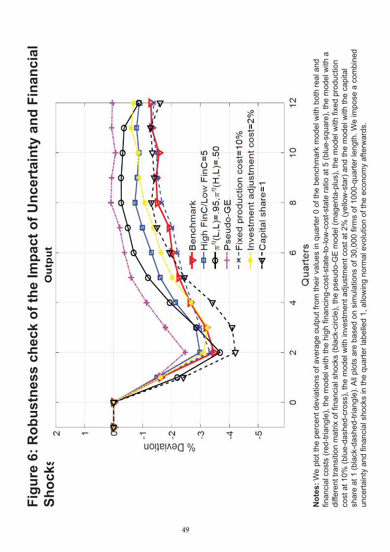
Figu

re 6

: Rob

ustn

ess

chec

k of

the

Impa

ct o

f Unc

erta

inty

and

Fin

anci

al

Shoc

ks

Not

es: W

e pl

ot th

e pe

rcen

t dev

iatio

ns o

f ave

rage

out

put f

rom

thei

r val

ues

in q

uarte

r 0 o

f the

ben

chm

ark

mod

el w

ith b

oth

real

and

fin

anci

al c

osts

(red

-tria

ngle

), th

e m

odel

with

the

high

fina

ncin

g-co

st-s

tate

-to-lo

w-c

ost-s

tate

ratio

at 5

(blu

e-sq

uare

), th

e m

odel

with

a

diffe

rent

tran

sitio

n m

atrix

of f

inan

cial

sho

cks

(bla

ck-c

ircle

), th

e ps

eudo

-GE

mod

el (m

agen

ta-p

lus)

, the

mod

el w

ith fi

xed

prod

uctio

n co

st a

t 10%

(blu

e-da

shed

-cro

ss),

the

mod

el w

ith in

vest

men

t adj

ustm

ent c

ost a

t 2%

(yel

low

-sta

r) an

d th

e m

odel

with

the

capi

tal

shar

e at

1 (b

lack

-das

hed-

trian

gle)

. All

plot

s ar

e ba

sed

on s

imul

atio

ns o

f 30,

000

firm

s of

100

0-qu

arte

r len

gth.

We

impo

se a

com

bine

d un

certa

inty

and

fina

ncia

l sho

cks

in th

e qu

arte

r lab

elle

d 1,

allo

win

g no

rmal

evo

lutio

n of

the

econ

omy

afte

rwar

ds.

s

49

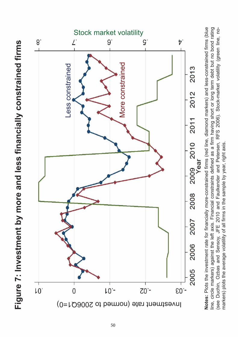
Figu

re 7

: Inv

estm

ent b

y m

ore

and

less

fina

ncia

lly c

onst

rain

ed fi

rms

Not

es:P

lots

the

inve

stm

entr

ate

forf

inan

cial

lym

ore-

cons

train

edfir

ms

(red

line,

diam

ond

mar

kers

)and

less

-con

stra

ined

firm

s(b

lue

line,

circ

lem

arke

rs)

agai

nstt

hele

ftax

is.F

inan

cial

cons

train

tsde

fined

asa

firm

havi

ngsh

orto

rlo

ngte

rmde

btbu

tno

bond

ratin

g(s

eeD

uchi

n,O

zbas

and

Sens

oy,

JFE

2010

and

Faul

kend

eran

dPe

ters

en,

RFS

2006

).St

ock-

mar

ket

vola

tility

(gre

enlin

e,no

-m

arke

rs)p

lots

the

aver

age

vola

tility

ofal

lfirm

sin

the

sam

ple

byye

ar,r

ight

axis

.

Investment rate (normed to 2006Q1=0)Stock market volatility

Less

con

stra

ined

Mor

e co

nstra

ined

50

Appendix For Online Publication

A Numerical algorithm

We use the value function iteration procedure to solve the firm’s maximization problemnumerically. We specify the two grids of 82 points for capital and 312 points for cash,respectively, with upper bounds k and n that are large enough to be non-binding. Thegrid for capital is constructed recursively given the pre-specified lower and upper bounds k

¯and k, following ki = ki−1/(1 − δ), where i = 1,...,s is the index of grids points. The gridfor cash is constructed recursively using a similar approach, following ni = ni−1/(1 + rn),where i = 1,...,s is the index of grids points given pre-specified lower and upper bounds n

¯and n. The advantage of this construction approach is that it does not require off-grid pointsinterpolation. For robustness check, we also construct a different grid of 60 points for cash,with upper bound n that is large enough to be non-binding. The grid for cash is constructedrecursively, that is, ni = ni−1 + cn1 exp(cn2(i − 2)), where i = 1,...,s is the index of gridspoints and cn1 and cn2 are two constants chosen to provide the desired number of grid pointsand two upper bound n, given pre-specified lower bounds n

¯. The advantage of this recursive

construction is that more grid points are assigned around n¯

, where the value function has mostof its curvature. Linear interpolation is used to obtain optimal investment and cash holdingthat do not lie directly on the grid points. We find two construction approaches producesimilar quantitative results.

We discretize the firm-specific productivity with two-state Markov process of time-varyingconditional volatility into a 5 (productivity level) by 2 grid. In all cases, the results are robustto finer grids for the level of productivity process as well. Once the discrete state space isavailable, the conditional expectation can be carried out simply as a matrix multiplication.Finally, we use a simple discrete global search routine in maximizing the firm’s problem.

B Data

Data used in the empirical analysis is described in detail in this section. Sources includeCompustat, CRSP, OptionMetrics, Bloomberg, CBOE, St. Louis Fed, and Baker, Bloom,and Davis (2016). Table A2 presents descriptive statistics of main variables used in the firm-level panel regressions. Our annual sample period begins in 1963 and ends in 2016.25

B.1 Company financial reports and realized stock return volatility

We draw financial information for US publicly held companies from Compustat. Sampleis annual from 1963 to December 2016. We use Compustat fiscal-year annual company datafrom balance sheet, income statement, and cash flow statement. Financial, utilities, and publicsector firms are excluded from the sample. In particular, we exclude firms with historical SICcodes in the range of 6000 to 6999, 4900 to 4999, and equal to or greater than 9000.26 When

25OLS and 2SLS regressions are run in STATA v.15 using the package REGHDFE.26In general we do not use the current or “header” SIC code of a company (which is time invariant

and only representative of the company’s industry at the time of Compustat data download), but rather

I

Compustat reports more than one annual data for the same-company in a given fiscal year (e.g.,when a company changes its fiscal-year end month) we drop the first chronologically datedobservations and keep only the last data for that fiscal year, ensuring only one data pointper firm-fiscal year. We drop any firm-year observations having zero or negative employment,total assets, and/or sales.

Our main empirical tests involve either variables in ratios, levels, and/or in changes fromone fiscal year to the next. To ensure that the latter changes are indeed annual, we requirea 12 month distance between fiscal-year end dates of accounting reports. Moreover, whenmeasuring changes from one year to the next we define the growth rate as in Davis andHaltiwanger (1992), where for any variable xt the growth rate is ∆xt = (xt − xt−1)/(12xt +12xt−1), which for positive values of xt and xt−1 yields growth rates bounded between -2 and

2. Moreover, whenever both xt and xt−1 are zero we set the corresponding growth rate equalto zero (which avoids losing information to undefined values and because in fact the growthrate is zero in this case).

Our set of dependent variables starts with capital formation. We measure firm investmentrate (implicitly the change in gross capital stock) as

CAPXi,t

Ki,t−1where K is net property plant

and equipment, and CAPX is capital expenditures. We bound investment rate above at 0.5and below at -0.10. For all other variables, we winsorize the levels, ratios, and growths everyfiscal semester at the 1 and 99 percentiles. Aside from investment, we also explore additionalreal outcomes which include employment, EMP in Compustat , Intangible Capital, definedas SG&A + R&D (sales, general and administration plus research and development), andcost of goods sold, COGS. Our set of financial outcomes include corporate payout definedas Payout = DV + PRSTKC , where DV is cash dividends and PRSTKC is purchase ofcommon and preferred stock from Compustat. Cash holdings is the level of cash and short-term investments, CHE. Total debt is Total Debt = DLC+DLTT , where DLC and DLTTare short-term and long-term debt from Compustat, respectively.

Our main set of firm-level controls includes the following variables (in levels). Stock Returnis a firm’s compounded fiscal-year return, using CRSP daily returns (including dividendsand adjusted for delisting, RET ) within the corresponding 12-month fiscal-year period.Tangibilityt = PPEGT/AT, where PPEGT is gross property, plant, and equipment andAT is total assets. Book leverage = (DLC + DLTT )/(DLC + DLTT + CEQ) , whereCEQ is Compustat common book equity. Tobin’s Q is computed as in Duchin, Ozbas, andSensoy (2010), Qi,t = (market value of assets) /(0.9 ∗ book assets+ 0.1 ∗ market value ofassets), where market value of assets is ( AT +ME+CEQ−TXDB ), ME is CRSP marketvalue of equity (i.e. stock price times shares outstanding), book assets is AT, and TXDB isdeferred taxes. We handle outliers in Tobin’s Q by bounding Q above at 10. Return on assets,ROAt = EBIT/AT , where EBIT is earnings before interest and tax. We further control forfirm size, defined as log SALE .

As for our main variable of interest firm-level uncertainty shocks, ∆σi,t, we measureuncertainty in two ways, realized and option-implied uncertainty. Realized uncertainty is

classify companies each year based on their historical industry SICH codes (i.e., standard industrialclassification -historical, from Compustat), or when missing in a given year we replace it with the closestbackward-looking non-missing historical code. We backfill any remaining codes using the first non-missingSICH code in the time-series. When none of the above are available we employ the firm’s current (header)SIC code for all years.

II

the annual volatility of the firm’s realized CRSP stock return. Specifically, we estimate itas the 12-month fiscal-year standard deviation of daily CRSP returns. We annualize thisstandard deviation by multiplying by the square root of 252 (average trading days in a year).This makes the standard deviation comparable to the annual volatility implied by call options,which we describe in the next subsection. We drop observations of firms with less than 200daily CRSP returns in a given fiscal year. Our sample uses securities appearing on CRSP forfirms listed in major US stock exchanges (EXCHCD codes 1,2, and 3 for NYSE, AMEX andthe Nasdaq Stock Market (SM)) and equity shares listed as ordinary common shares (SHRCD10 or 11).

B.2 Implied volatility

Although our main measure of firm-level uncertainty is realized annual stock return volatility,we further proxy for uncertainty by using OptionMetrics’ 365-day implied volatility of at-the-money-forward call options.

OptionMetrics provides daily implied volatility from January 1996 onward for securitieswith exchange-traded equity options. Each security has a corresponding series of call andput options which differ in their expiration dates and strike prices. For each of these options,OptionMetrics imputes an implied volatility for each trading day using the average of theend-of-day best bid and offer price quotes. To be consistent with the annual Compustat dataused throughout, our main tests focus only on 365-day implied volatility. We further restrictour analysis to call options. Note that a call option and a put option on a given underlyingasset with the same strike price and expiration date have the same implied volatilities; thedifference in their prices comes from the fact that interest rates and dividends affect the valueof call and put options in opposite directions. Therefore, our principal proxy for uncertaintyis 365-day implied volatility of at-the-money-forward call options.

B.3 Currency exchange rates and implied volatility

We use bilateral exchange rate data from the Federal Reserve Board. Although there is a largenumber of bilateral currencies available, we restrict our attention to the exchange rates betweenthe U.S. dollar and the 7 “major” currencies used by the Board in constructing the nominal andreal trade-weighted U.S. dollar Index of Major Currencies27.These include the Euro, Canadiandollar, Japanese Yen, British Pound, Swiss Franc, Australian Dollar, and Swedish Krona.Each one of these trades widely in currency markets outside their respective home areas, and(along with the U.S. dollar) are referred to by the Board staff as major currencies. Thesedaily currency spot prices are used in the daily regression described in equation 14 .

In addition to the daily currency prices, our instrumental variables approach furtherrequires measures of forward-looking implied volatility for each of the 7 currencies. For thesewe use daily data on three-month implied exchange rate volatilities for each bilateral rate,from Bloomberg. Specifically, we extract these data using the VOLC function available atBloomberg terminals.

27See: http://www.federalreserve.gov/pubs/bulletin/2005/winter05_index.pdf .

III

B.4 Energy prices and implied volatility

We employ shocks to oil price as a general proxy for energy prices. We collect oil price andimplied volatility data from Bloomberg. In particular, Bloomberg provides price and 30-day implied volatility data for one-month crude oil futures. Specifically, we use data on theNew York Mercantile Exchange Division’s light, sweet crude oil futures contract (BloombergCL1). This contract is the world’s most liquid, largest-volume futures contract on a physicalcommodity. The contract size is 1,000 U.S. barrels and delivery occurs in Cushing, Oklahoma.Our data on oil futures implied volatility starts in 1Q 2003.

As with exchange rates above, we construct our annual industry-by-year instrument for oilby averaging the daily implied volatility data for oil over the corresponding 252-day backward-looking window for each fiscal-year month-end date of a company.

B.5 Timing alignment of firm-level volatility and instruments

Most of our empirical analysis examines the effect of 1-year lagged changes in annual firm-leveluncertainty ∆σi,t−1 on the changes in both real and financial outcomes ∆yi,t. In defining thechange in any variable xt, growth is ∆xt = (xt − xt−1)/(12xt + 1

2xt−1) . This applies to our

outcomes ∆yi,t, lagged instruments for energy prices, exchange rates, treasuries, and policy

uncertainty,| βc,weightedj | ·∆σct−1, and also our main uncertainty measure of the lagged growthin firm i′s realized annual volatility, ∆σi,t−1. Given that our regressions are predictive fromyear t − 1 to year t, our first-stage 2SLS regressions involve a regression of firms’ laggeduncertainty shock ∆σi,t−1 = (σi,t−1 − σi,t−2)/(

12σi,t−1 + 1

2σi,t−2) on the 10 lagged composite

exposures to aggregate uncertainty shocks IV ct−1 = | βc,weightedj | ·∆σct−1 where for instrument

c the growth in the lagged uncertainty shock is ∆σct−1 = (σct−1 − σct−2)/(12σct−1 + 1

2σct−2) , and

| βc,weightedj | is the significance-weighted cross-industry exposure estimated 36 months priorto the firm’s fiscal-year end month of the dependant variable, ∆yi,t.

Taking into account that daily data on implied volatility of treasuries (TYVIX TheCboe/CBOT ) starts in 1Q 2003, our main 2SLS regression sample containing the full setof 10 instruments (oil, 7 exchange rates, 10-year treasuries, and policy) effectively starts forany firm in fiscal year 2006. Our sample ends in December 2016.

IV

Table A1

Coefficient on changes in volatility for real and financial variables

Real Financial

I/K ∆Emp ∆Cash Div/K

A: Benchmark

∆Volatility -0.080 -0.028 0.487 -0.012

B: H/L = 5

∆Volatility -0.090 -0.031 0.462 -0.007

C: Different transition matrix of ηt∆Volatility -0.086 -0.030 0.465 -0.009

D: Pseudo-GE

∆Volatility -0.053 -0.020 0.610 -0.020

E: F = 0.10

∆Volatility -0.071 -0.025 0.820 -0.018

F:ck= 0.02

∆Volatility -0.093 -0.031 0.169 -0.004

G:α = 1

∆Volatility -0.086 na -0.082 -0.002

This table reports the model regression results of real and financial variables on volatility growth. The reportedstatistics in the model are from simulated data with 3000 firms and 200 quarterly observations. We reportthe cross-simulation averaged annual moments. I/K is the investment rate, ∆Emp is the employment growth,∆Cash is the cash growth rate, and Div/K is the ratio of dividend to capital in the model and cash dividendplus repurchase to total assets in the data. Panel A is the benchmark calibration. Panels B lowers the highfinancing-cost-state-to-low-cost-state ratio (ηH/ηL ) to 5 while keeping the low financial cost state ηL = 0.005.Panel C sets the transition probabilities of financial shocks of πσL,H = 0.05 and πσH,H = 0.5. Panel D is thepseudo-GE model with interest rates, prices and wages as functions of uncertainty shock. Panel E is the modelwith smaller fixed production cost F = 0.10. Panel F is the model with bigger investment adjustment costck = 0.02. Panel G is the model with the share of capital α = 1. All the regressions include firm and timefixed effects and all results for the model are significant at the 1% level with firm-clustered standard errors.

V

Table A2

Descriptive statistics

Variables in 2SLS Obs. Mean S. Dev P1 P10 P50 P90 P99

Dependent

Investment Rate 125,596 0.248 0.152 0.012 0.067 0.215 0.500 0.500

∆Employment 125,690 0.026 0.231 -0.765 -0.192 0.021 0.258 0.744

∆Intangible Cap. Invest. 66,977 0.077 0.198 -0.535 -0.137 0.077 0.292 0.642

∆Cost of Goods Sold 126,913 0.080 0.283 -0.929 -0.177 0.080 0.342 1.024

∆Debt Total 126,022 0.046 0.669 -2.000 -0.514 0.000 0.738 2.000

∆Payout 126,925 0.066 0.919 -2.000 -1.185 0.000 1.482 2.000

∆Cash Holdings 126,899 0.043 0.702 -1.727 -0.839 0.043 0.934 1.797

Independent

∆Realized Volatility 126,925 -0.001 0.303 -0.673 -0.376 -0.012 0.386 0.780

∆Implied Volatility 26,759 -0.015 0.200 -0.435 -0.259 -0.026 0.247 0.513

Book Leverage 125,460 0.322 0.279 0.000 0.000 0.291 0.672 1.287

Stock Return 126,925 0.176 0.674 -0.765 -0.458 0.066 0.847 2.781

Log Sales 126,680 5.092 2.140 -0.246 2.452 5.043 7.887 9.979

Return on Assets 126,914 0.049 0.181 -0.784 -0.108 0.082 0.194 0.326

Tangibility 126,545 0.550 0.363 0.037 0.140 0.479 1.057 1.657

Tobin’s Q 125,795 1.482 0.833 0.569 0.791 1.215 2.539 4.690

Instruments

∆Vol Exposure Cad 44,220 3e-04 0.006 -0.015 -0.001 0.000 0.002 0.020

∆Vol Exposure Euro 43,773 -2e-04 0.011 -0.030 -0.004 0.000 0.001 0.047

∆Vol Exposure Jpy 50,607 1e-04 0.005 -0.011 -0.001 0.000 0.000 0.015

∆Vol Exposure Aud 50,607 3e-05 0.006 -0.018 -0.003 0.000 0.003 0.022

∆Vol Exposure Sek 44,220 2e-04 0.007 -0.021 -0.004 0.000 0.002 0.032

∆Vol Exposure Chf 50,607 1e-04 0.009 -0.021 -0.003 0.000 0.001 0.032

∆Vol Exposure Gbp 50,607 1e-04 0.005 -0.014 -0.001 0.000 0.000 0.018

∆Vol Exposure Oil 29,016 6e-05 0.011 -0.040 -0.001 0.000 0.001 0.029

∆Vol Exposure Policy 50,607 3e-07 2e-05 -8e-05 0.000 0.000 0.000 8e-05

∆Vol Expos.Treasury 29,195 -0.637 8.503 -32.100 -4.564 0.000 2.286 26.640

This table presents summary statistics of all main variables used in the empirical panel regression analysis.Sample period is annual from 1963 to 2016. Notation ∆x stands for growth rate of variable x, defined as(xt − xt−1)/(0.5 ∗ xt + 0.5 ∗ xt−1), standard deviation is S. Dev., while. P1, P10, P50, P90 and P99 standfor the 1, 10, 50, 90 and 99 percentiles, respectively. Data sources include CRSP, Compustat, OptionMetrics,Bloomberg, CBOE, St. Louis Fed, and Baker, Bloom, and Davis (2016). See sections 4 and 5 for the detailson the construction of variables.

VI

Table

A3

2SL

SSensi

tivit

yto

indiv

idual

inst

rum

ents

(1)

(2)

(3)

(4)

(5)

(6)

(7)

(8)

(9)

(10)

IVD

rop

ped

Non

eC

adE

uro

Jpy

Au

dS

ekC

hf

Gb

pP

olic

yO

il+

Tre

asu

ries

Rea

lV

aria

ble

s

Inve

stm

ent

Rat

e i,t

-0.0

30**

*-0

.032*

**-0

.029

***

-0.0

30**

*-0

.034

***

-0.0

35**

*-0

.030

***

-0.0

30**

*-0

.031

***

-0.0

36**

∆In

tan

g.C

ap

.In

vest

. i,t

-0.0

36**

-0.0

35*

-0.0

34*

-0.0

38**

-0.0

40**

-0.0

30†

-0.0

42**

-0.0

40**

-0.0

33*

-0.0

35†

∆E

mp

loym

ent i,t

-0.0

11-0

.009

-0.0

08-0

.011

-0.0

10-0

.037

-0.0

17-0

.010

-0.0

090.0

16

Fin

anci

alV

aria

ble

s

∆D

ebt

Tot

ali,t

-0.1

68**

-0.1

54*

*-0

.156

**-0

.167

**-0

.200

***

-0.2

03**

*-0

.163

**-0

.168

**-0

.170

**-0

.218**

∆P

ayou

t i,t

-0.3

10**

*-0

.331*

**-0

.291

***

-0.3

06**

*-0

.379

***

-0.2

86**

-0.2

74**

-0.3

03**

-0.3

02**

-0.4

87***

∆C

ash

Hol

din

gsi,t

0.166

**0.

153*

*0.

164*

*0.

159*

*0.

202*

**0.

175*

*0.

124*

0.15

7**

0.16

1**

0.2

65**

1st

mom

ent

10IV

i,t−

1Y

esY

esY

esY

esY

esY

esY

esY

esY

esY

es

Fir

m,

tim

eF

EY

esY

esY

esY

esY

esY

esY

esY

esY

esY

es

SE

clu

ster

(3S

IC)

Yes

Yes

Yes

Yes

Yes

Yes

Yes

Yes

Yes

Yes

Inve

stm

ent

Rat

eS

tats

Ob

serv

atio

ns

28,1

3228

,132

28,1

3228

,132

28,1

3228

,132

28,1

3228

,132

28,1

3242,3

88

F1s

tst

age

Cra

gg-D

171.

1178

.718

2.8

187.

516

1.6

150.

817

318

2.4

184.

999.1

7

F1s

tst

age

Kle

ib.-

P.

17.

5719

.84

19.3

518

.34

14.0

917

.88

18.4

016

.97

18.3

112.0

9

p-v

alS

arga

n–H

ans

J0.9

550.

946

0.93

90.

921

0.96

10.

950

0.92

10.

938

0.92

00.9

92

Th

ista

ble

pre

sents

2SL

Sm

ult

ivar

iate

regr

essi

onre

sult

sfo

ral

lou

rm

ain

real

and

fin

anci

alou

tcom

eva

riab

les

(wit

hfu

llse

tof

contr

ols)

wh

enw

ed

rop

ind

ivid

ual

inst

rum

ents

one

ata

tim

efr

omou

rb

ench

mar

kse

tof

10in

stru

men

tal

vari

able

s(I

Vs)

.In

the

last

colu

mn

(10)

we

dro

pb

oth

oil

an

dtr

easu

ryIV

sas

thes

eco

nst

rain

the

star

tof

the

sam

ple

tofi

scal

year

2006

,w

her

eas

kee

pin

gon

lycu

rren

cies

and

pol

icy

IVs

allo

wan

add

itio

nal

4ye

ars

of

pan

eld

ata

-wit

hfi

rst

fisc

alye

arof

dep

end

ent

vari

able

star

tin

gin

2002

.S

amp

lep

erio

den

ds

inD

ecem

ber

2016

.T

he

coeffi

cien

tan

dst

atis

tics

rep

ort

edin

(1)

are

from

the

ben

chm

ark

2SL

Sm

ult

ivar

iate

regr

essi

onon

lagg

edfi

rm-l

evel

real

ized

vola

tili

tysh

ock

sp

rese

nte

din

colu

mn

(3)

acro

ssT

ab

les

3,

5,

an

d6.

Th

est

atis

tics

un

der

”Inve

stm

ent

Rat

eS

tats

”co

rres

pon

dto

the

1st

stag

ere

sult

sof

the

mu

ltiv

aria

te2S

LS

regr

essi

onof

inve

stm

ent

rate

on

lagged

chan

gein

real

ized

vola

tili

tyan

dm

ain

set

ofla

gge

dle

vel

contr

ols.

1st

Sta

gest

atis

tics

for

oth

erre

alan

dfi

nan

cial

esti

mat

ion

sar

ela

rgel

yco

mp

ara

ble

toth

eir

ben

chm

ark

spec

ifica

tion

sw

ith

the

full

set

ofin

stru

men

ts.

Fir

man

dca

len

dar

-yea

rfi

xed

effec

tsin

clu

ded

.Sta

nd

ard

erro

rscl

ust

ered

at

the

3d

igit

SIC

ind

ust

ry.

To

teas

eou

tth

eim

pac

tof

2nd

mom

ent

unce

rtai

nty

shock

sw

eal

soin

clu

de

asco

ntr

ols

the

lagg

edex

pos

ure

toth

ere

turn

on

each

of

the

10ag

greg

ate

inst

rum

ents

(i.e

.,1s

tm

om

ent

shock

s).

Dat

aav

aila

bil

ity

onim

pli

edvo

lati

lity

oftr

easu

ries

and

oil

rest

rict

the

star

tof

the

2SL

Ssa

mp

leto

fisc

alyea

r20

06.

Sta

tist

ical

sign

ifica

nce

:**

*p<

0.01

,**

p<

0.05

,*

p<

0.1,†

p<

0.15

.t-

stat

isti

csar

ein

par

enth

eses

.S

eese

ctio

n4

for

dat

adet

ails.

VII

Table

A4

2SL

SR

obust

ness

test

s

(1)

(2)

(3)

(4)

(5)

(1A

)(2

A)

(3A

)(4

A)

(5A

)

Vola

tili

tyIn

stru

mente

dR

eali

zed

Rea

lize

dR

eali

zed

Rea

lize

dR

eali

zed

Imp

lied

Imp

lied

Imp

lied

Imp

lied

Imp

lied

Real

Vari

ab

les

Inve

stm

ent

Rat

e i,t

-0.0

33**

*-0

.030

***

-0.0

30**

*-0

.031

***

-0.0

30**

*-0

.082

*-0

.077

**-0

.083

**-0

.081**

-0.0

83**

∆In

tan

gib

leC

ap

.In

vest

. i,t

-0.0

42**

-0.0

34*

-0.0

32*

-0.0

33*

-0.0

29†

-0.0

79-0

.036

-0.0

44-0

.036

-0.0

26

∆E

mp

loym

ent i,t

-0.0

05-0

.010

-0.0

12-0

.011

-0.0

110.

045

-0.0

39-0

.046

-0.0

45

-0.0

41

Fin

an

cia

lV

ari

ab

les

∆D

ebt

Tot

ali,t

-0.1

84**

-0.1

67**

-0.1

70**

-0.1

69**

-0.1

68**

*-0

.843

***

-0.6

02**

*-0

.623

***

-0.6

20***

-0.6

12***

∆P

ayou

t i,t

-0.3

58**

-0.2

95**

-0.3

33**

*-0

.313

***

-0.3

20**

*-1

.419

**-0

.798

**-0

.927

***

-0.8

47***

-0.8

77***

∆C

ash

Hol

din

gsi,t

0.18

3**

0.16

0**

0.15

4**

0.16

4**

0.15

1**

0.81

8**

0.56

7***

0.58

2***

0.5

69***

0.5

79***

Lev

erag

e-ad

just

ed∆

Vol

atil

ityi,t−

1Y

esY

es

Mai

nfi

rm-l

evel

contr

ols i,t−

1Y

esY

esY

esY

esY

esY

esY

esY

esY

esY

es

Cov

aria

nce

w/

mar

keti,t−

1Y

esY

esY

esY

es

Fin

anci

alco

nst

rain

tin

dex

esi,t−

1Y

esY

esY

esY

es

S&

Pcr

edit

rati

ngsi,t−

1Y

esY

esY

esY

es

1st

mom

ent

contr

ols

10IV

i,t−

1Y

esY

esY

esY

esY

esY

esY

esY

esY

esY

es

Fir

m,

tim

eF

EY

esY

esY

esY

esY

esY

esY

esY

esY

esY

es

SE

clu

ster

ing

(3SIC

ind

ust

ry)

Yes

Yes

Yes

Yes

Yes

Yes

Yes

Yes

Yes

Yes

Invest

ment

Rate

Sta

ts

Ob

serv

atio

ns

28,0

7828

,132

28,0

5828

,132

28,0

5817

,358

17,3

9117

,345

17,3

91

17,3

45

F1s

tst

age

Cra

gg-D

onal

dW

ald

96.7

218

2.6

170.

317

118

1.8

12.5

264

.958

.17

59.0

665.0

5

F1s

tst

age

Kle

iber

gen

-Paa

pW

ald

14.3

019

.39

17.5

017

.61

19.3

24.

8913

.04

11.3

811.2

813.3

1

p-v

alS

arga

n–H

anse

nJ

Ch

i-sq

0.8

910.

955

0.92

80.

950

0.92

20.

846

0.94

90.

938

0.9

50

0.9

34

Th

ista

ble

pre

sents

2SL

Sro

bu

stn

ess

resu

lts

for

allou

rre

alan

dfi

nan

cial

outc

ome

vari

able

sex

amin

edin

mai

nT

able

s3,

5,an

d6.

All

spec

ifica

tion

sin

clu

de

full

set

ofco

ntr

ols.

Inco

lum

ns

(1)

and

(1A

)w

ein

vest

igat

ew

het

her

the

resu

lts

are

rob

ust

toad

just

ing

vola

tili

tyby

firm

leve

rage

,i.

e.,σi,t·

Ei,t

Ei,t

+D

i,t

wh

ereE

isb

ook

equ

ity

andD

isto

tald

ebt.

Ad

dit

ion

alco

ntr

ols

incl

ud

e:co

vari

ance

w/

mar

ket

,w

hic

had

ds

firm

lagg

edC

AP

Mb

eta,

fin

anci

alco

nst

rain

tin

dex

es,

wh

ich

add

ase

tof

6la

gge

dfi

rm-l

evel

contr

ols

for

firm

fin

anci

alco

nst

rain

ts.

Th

ese

incl

ud

eth

ela

gged

Wh

ited

-Wu

ind

ex,

lagg

edS

Ain

dex

of

Had

lock

and

Pie

rce

(201

0),

the

Kap

lan-Z

inga

les

ind

ex,

reci

pro

cal

ofto

tal

asse

ts,

reci

pro

cal

ofem

plo

yees

,an

dre

cip

roca

lof

age.

Th

eS

&P

cred

itra

tin

gs

colu

mn

furt

her

add

sa

full

set

ofd

um

mie

sb

ase

don

ever

yp

ossi

ble

cred

itra

tin

gca

tego

rygi

ven

by

S&

Pon

lon

g-te

rmd

ebt.

Om

itte

dd

um

my

isfo

rn

ocr

edit

rati

ngs

.F

irm

and

cale

nd

ar-y

ear

fixed

effec

tsar

ein

clu

ded

.S

tan

dar

der

rors

clu

ster

edat

the

3-d

igit

SIC

ind

ust

ry.

Sta

tist

ical

sign

ifica

nce

:***

p<

0.01

,**

p<

0.05

,*

p<

0.1,†

p<

0.15

.t-

stati

stic

sar

ein

par

enth

eses

.S

eese

ctio

n4

for

dat

ad

etai

ls.

VIII

Table A5

Investment rate, using same panel across specifications

(1) (2) (3) (4) (5) (6)

Investment ratei,t OLS IV IV OLS IV IV

Realized Realized Realized Implied Implied Implied

∆Volatilityi,t−1 -0.033*** -0.086*** -0.029** -0.079*** -0.225*** -0.078**

(-4.642) (-3.527) (-2.470) (-7.447) (-4.184) (-2.454)

Book Leveragei,t−1 -0.040*** -0.037***

(-6.203) (-5.583)

Stock Returni,t−1 0.006** 0.005*

(2.194) (1.808)

Log Salesi,t−1 -0.023*** -0.022***

(-5.419) (-5.290)

Return on Assetsi,t−1 0.138*** 0.132***

(4.087) (3.910)

Tangibilityi,t−1 -0.126*** -0.123***

(-3.491) (-3.355)

Tobin’s Qi,t−1 0.055*** 0.054***

(8.089) (8.341)

1st moment 10IVi,t−1 No No Yes No No Yes

Firm, time FE Yes Yes Yes Yes Yes Yes

SE cluster(3SIC) Yes Yes Yes Yes Yes Yes

Observations 17,391 17,391 17,391 17,391 17,391 17,391

F 1st st. Cragg-D 131.5 140.1 77.94 58.59

F 1st st. Kleib.-P 15.40 15.29 14.99 11.14

p-val Sargan–H J 0.590 0.918 0.659 0.950

This table presents all investment rate regression results shown in main Table 3 but holding the sampleof firm-time observations fixed across specifications. The sample is restricted to firms that have both non-missing lagged realized and implied volatilities every fiscal year. Investment rate at fiscal year t is defined asIt/Kt−1 (capx/lagged net property plant & equipment from Compustat). Sample period is from 1963 to 2016.Specifications 1 and 4 are OLS while all others 2SLS. We instrument lagged changes in firm-level volatilitywith industry-level (3SIC) exposure to 10 aggregate lagged uncertainty shocks. These include the laggedexposure to annual changes in expected volatility of energy, currencies, and 10-year treasuries and economicpolicy uncertainty from Baker, Bloom, and Davis (2016). Annual realized volatility is the 12-month standarddeviation of daily stock returns from CRSP. Implied volatility is the annual average of daily (365-day) impliedvolatility of at-the-money-forward call options from OptionMetrics. Regressors lagged by 1-year. Both firmand calendar-year fixed effects are included. Standard errors are clustered at the 3-digit SIC industry. Totease out the impact of 2nd moment uncertainty shocks we also include as controls the lagged exposure tochanges in the return on each of the 10 aggregate instruments (i.e., 1st moment shocks). Data availabilityon implied volatility of treasuries and oil restrict the start of the 2SLS sample to fiscal year 2006. Statisticalsignificance: *** p<0.01, ** p<0.05, * p<0.1, † p<0.15. t-statistics are in parentheses. See section 4 for data.

IX

Table A6

Uncertainty effects on corporate dividend payout ratios

(1) (2) (3) (4) (5) (6)

Payout ratioi,t OLS IV IV OLS IV IV

Realized Realized Realized Implied Implied Implied

∆Volatilityi,t−1 -0.004*** -0.019*** -0.009* -0.016*** -0.059*** -0.037**

(-10.734) (-3.893) (-1.658) (-6.650) (-4.237) (-2.072)

Book Leveragei,t−1 -0.029*** -0.036***

(-4.028) (-3.226)

Stock Returni,t−1 -0.003*** -0.005***

(-5.102) (-3.966)

Log Salesi,t−1 0.002 0.004

(0.876) (0.850)

Return on Assetsi,t−1 0.034*** 0.036***

(4.585) (3.019)

Tangibilityi,t−1 -0.006 0.002

(-1.186) (0.261)

Tobin’s Qi,t−1 0.014*** 0.018***

(5.593) (4.268)

1st moment 10IVi,t−1 No No Yes No No Yes

Firm, time FE Yes Yes Yes Yes Yes Yes

SE cluster(3SIC) Yes Yes Yes Yes Yes Yes

Observations 125,532 28,471 28,173 26,153 17,596 17,408

F 1st st. Cragg-D 158.4 171.8 78.54 58.56

F 1st st. Kleib.-P 18.43 17.48 14.96 11.16

p-val Sargan–H J 0.542 0.326 0.338 0.262

Table presents OLS and 2SLS annual regression results of firm corporate dividend payout ratios on 1-yearlagged changes in firm-level volatility and lagged level of firm-level controls. Dividend payout ratio at fiscal

year t is defined asPayouti,tATi,t−1

, where Payout = DV + PRSTKC, DV is cash dividends and PRSTKC is

purchase of common and preferred stock, and AT is total assets from Compustat. Sample period is from 1963to 2016. Specifications 1 and 4 are OLS while all others 2SLS. We instrument lagged changes in firm-levelvolatility with industry-level (3SIC) exposure to 10 aggregate lagged uncertainty shocks. These include thelagged exposure to annual changes in expected volatility of energy, currencies, and 10-year treasuries andeconomic policy uncertainty from Baker, Bloom, and Davis (2016). Annual realized volatility is the 12-monthstandard deviation of daily stock returns from CRSP. Implied volatility is the annual average of daily (365-day)implied volatility of at-the-money-forward call options from OptionMetrics. Regressors lagged by 1-year. Bothfirm and calendar-year fixed effects are included. Standard errors are clustered at the 3-digit SIC industry.To tease out the impact of 2nd moment uncertainty shocks we also include as controls the lagged exposureto changes in the return on each of the 10 aggregate instruments (i.e., 1st moment shocks). Data availabilityon implied volatility of treasuries and oil restrict the start of the 2SLS sample to fiscal year 2006. Statisticalsignificance: *** p<0.01, ** p<0.05, * p<0.1, † p<0.15. t-statistics are in parentheses. See section 4 for data.

X

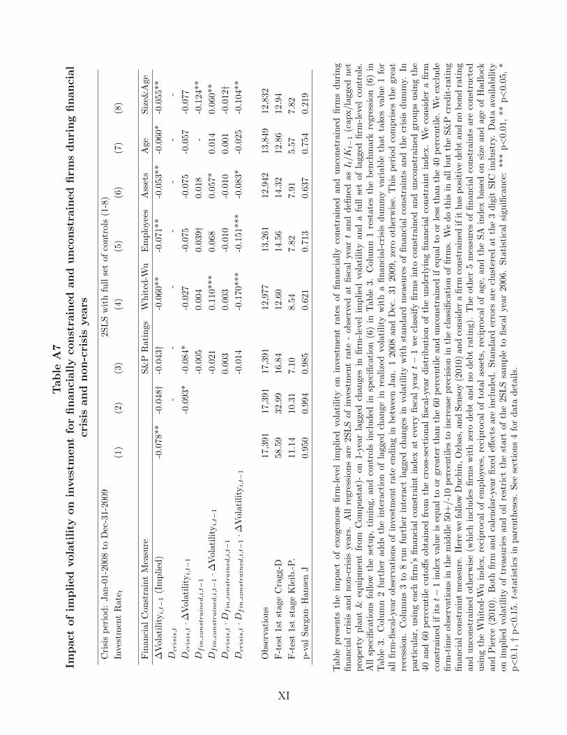
Table

A7

Impact

of

implied

vola

tility

on

invest

ment

for

financi

ally

const

rain

ed

and

unco

nst

rain

ed

firm

sduri

ng

financi

al

cris

isand

non-c

risi

syears

Cri

sis

per

iod

:Jan

-01-2

008

toD

ec-3

1-20

092S

LS

wit

hfu

llse

tof

contr

ols

(1-8

)

Inve

stm

ent

Rat

e t(1

)(2

)(3

)(4

)(5

)(6

)(7

)(8

)

Fin

anci

alC

onst

rain

tM

easu

reS

&P

Rat

ings

Wh

ited

-Wu

Em

plo

yees

Ass

ets

Age

Siz

e&A

ge

∆V

olat

ilit

yi,t−

1(I

mp

lied

)-0

.078

**-0

.048†

-0.0

43†

-0.0

60**

-0.0

71**

-0.0

53**

-0.0

60*

-0.0

55**

Dcrisis,t

--

--

--

-

Dcrisis,t·∆

Vola

tili

tyi,t−

1-0

.093

*-0

.084

*-0

.027

-0.0

75-0

.075

-0.0

57-0

.077

Dfin

constrained,i,t−

1-0

.005

0.00

40.

039†

0.01

8-

-0.1

24**

Dfin

constrained,i,t−

1·∆

Vol

atil

ityi,t−

1-0

.021

0.11

0***

0.06

80.

057*

0.01

40.0

60**

Dcrisis,t·D

fin

constrained,i,t−

10.

003

0.00

3-0

.010

-0.0

100.

001

-0.0

12†

Dcrisis,t·D

fin

constrained,i,t−

1·∆

Vola

tili

tyi,t−

1-0

.014

-0.1

70**

*-0

.151

***

-0.0

83*

-0.0

25-0

.104**

Ob

serv

atio

ns

17,3

9117

,391

17,3

9112

,977

13,2

6112

,942

13,8

4912,8

32

F-t

est

1st

stag

eC

ragg

-D58

.59

32.9

916

.84

12.6

014

.56

14.3

212

.86

12.9

4

F-t

est

1st

stag

eK

leib

.-P

.11

.14

10.3

17.

108.

547.

827.

915.

577.8

2

p-v

alS

arga

n–H

anse

nJ

0.95

00.

994

0.98

50.

621

0.71

30.

637

0.75

40.2

19

Tab

lep

rese

nts

the

imp

act

ofex

ogen

ou

sfi

rm-l

evel

imp

lied

vola

tili

tyon

inves

tmen

tra

tes

offi

nan

cial

lyco

nst

rain

edan

du

nco

nst

rain

edfi

rms

du

rin

gfi

nan

cial

cris

isan

dn

on

-cri

sis

years

.A

llre

gres

sion

sar

e2S

LS

ofin

vest

men

tra

te-

obse

rved

atfi

scal

yeart

and

defi

ned

asI t/K

t−1

(cap

x/la

gged

net

pro

per

typ

lant

&eq

uip

men

tfr

omC

omp

ust

at)

-on

1-yea

rla

gged

chan

ges

infi

rm-l

evel

imp

lied

vol

atilit

yan

da

full

set

ofla

gged

firm

-lev

elco

ntr

ols

.A

llsp

ecifi

cati

ons

foll

owth

ese

tup

,ti

min

g,an

dco

ntr

ols

incl

ud

edin

spec

ifica

tion

(6)

inT

able

3.C

olu

mn

1re

stat

esth

eb

ench

mar

kre

gre

ssio

n(6

)in

Tab

le3.

Col

um

n2

furt

her

add

sth

ein

tera

ctio

nof

lagg

edch

ange

inre

aliz

edvo

lati

lity

wit

ha

fin

anci

al-c

risi

sd

um

my

vari

able

that

takes

valu

e1

for

all

firm

-fisc

al-y

ear

obse

rvat

ion

sof

inve

stm

ent

rate

end

ing

inb

etw

een

Jan

.1

2008

and

Dec

.31

2009

,ze

root

her

wis

e.T

his

per

iod

com

pri

ses

the

gre

at

rece

ssio

n.

Col

um

ns

3to

8ru

nfu

rth

erin

tera

ctla

gged

chan

ges

invol

atil

ity

wit

hst

and

ard

mea

sure

sof

fin

anci

alco

nst

rain

tsan

dth

ecr

isis

du

mm

y.In

par

ticu

lar,

usi

ng

each

firm

’sfi

nan

cial

con

stra

int

ind

exat

ever

yfi

scal

yea

rt−

1w

ecl

assi

fyfi

rms

into

con

stra

ined

and

un

con

stra

ined

grou

ps

usi

ng

the

40an

d60

per

centi

lecu

toff

sob

tain

edfr

omth

ecr

oss-

sect

ion

alfi

scal

-yea

rd

istr

ibu

tion

ofth

eu

nd

erly

ing

fin

anci

alco

nst

rain

tin

dex

.W

eco

nsi

der

afi

rmco

nst

rain

edif

itst−

1in

dex

valu

eis

equ

alto

orgr

eate

rth

anth

e60

per

centi

lean

du

nco

nst

rain

edif

equ

alto

or

less

than

the

40p

erce

nti

le.

We

excl

ud

efi

rm-t

ime

obse

rvat

ion

sin

the

mid

dle

50+

/-10

per

centi

les

toin

crea

sep

reci

sion

inth

ecl

assi

fica

tion

offi

rms.

We

do

this

inal

lb

ut

the

S&

Pcr

edit

-rati

ng

fin

anci

alco

nst

rain

tm

easu

re.

Her

ew

efo

llow

Du

chin

,O

zbas

,an

dS

enso

y(2

010)

and

con

sid

era

firm

con

stra

ined

ifit

has

pos

itiv

ed

ebt

and

no

bon

dra

tin

gan

du

nco

nst

rain

edot

her

wis

e(w

hic

hin

clu

des

firm

sw

ith

zero

deb

tan

dn

od

ebt

rati

ng)

.T

he

oth

er5

mea

sure

sof

fin

anci

alco

nst

rain

tsar

eco

nst

ruct

edu

sin

gth

eW

hit

ed-W

uin

dex

,re

cip

roca

lof

emp

loye

es,

reci

pro

cal

ofto

tal

asse

ts,

reci

pro

cal

ofag

e,an

dth

eS

Ain

dex

bas

edon

size

and

age

of

Had

lock

and

Pie

rce

(201

0).

Bot

hfi

rman

dca

len

dar

-yea

rfi

xed

effec

tsar

ein

clu

ded

.S

tan

dar

der

rors

are

clu

ster

edat

the

3d

igit

SIC

ind

ust

ry.

Dat

aav

ail

abil

ity

onim

pli

edvo

lati

lity

oftr

easu

ries

and

oil

rest

rict

the

star

tof

the

2SL

Ssa

mp

leto

fisc

alye

ar20

06.

Sta

tist

ical

sign

ifica

nce

:**

*p<

0.01

,**

p<

0.0

5,

*p<

0.1,†

p<

0.15

.t-

stat

isti

csin

par

enth

eses

.S

eese

ctio

ns

4fo

rd

ata

det

ails

.

XI