NBER WORKING PAPER SERIES THE DISTRIBUTION OF COVID-19 ...

We are extremely

NBER WORKING PAPER SERIES

THE DISTRIBUTION OF COVID-19 RELATED RISKS

Patrick BaylisPierre-Loup Beauregard

Marie ConnollyNicole Fortin

David A. GreenPablo Gutierrez Cubillos

Sam GyetvayCatherine Haeck

Timea Laura MolnarGaëlle Simard-Duplain

Henry E. SiuMaria teNyenhuis

Casey Warman

Working Paper 27881http://www.nber.org/papers/w27881

NATIONAL BUREAU OF ECONOMIC RESEARCH 1050 Massachusetts Avenue

Cambridge, MA 02138October 2020

We are extremely grateful to the dedicated set of people at Statistics Canada who made this work possible: Marc St. Denis, Cindy Cook, Andrew Heisz, Kelly Cranswick, Monica Pereira, Bin Hu, Adam Howe, Gabrielle Beaudoin, Jacques Fanteux, Lynn Barr-Telford, and Anil Arora. We are particularly grateful to Reka Gustafson at the BC Centre for Disease Control for her insight and advice, and to Tony Bonen and the Labour Market Information Council for support. We wish to thank CIRANO for financial support. Molnar thanks Analysis Group for supporting her pro bono involvement in a previous stage of this collaboration. The views expressed herein are those of the authors and do not necessarily reflect the views of the National Bureau of Economic Research or the Bank of Canada.

NBER working papers are circulated for discussion and comment purposes. They have not been peer-reviewed or been subject to the review by the NBER Board of Directors that accompanies official NBER publications.

© 2020 by Patrick Baylis, Pierre-Loup Beauregard, Marie Connolly, Nicole Fortin, David A. Green, Pablo Gutierrez Cubillos, Sam Gyetvay, Catherine Haeck, Timea Laura Molnar, Gaëlle Simard-Duplain, Henry E. Siu, Maria teNyenhuis, and Casey Warman. All rights reserved. Short sections of text, not to exceed two paragraphs, may be quoted without explicit permission provided that full credit, including © notice, is given to the source.

The Distribution of COVID-19 Related RisksPatrick Baylis, Pierre-Loup Beauregard, Marie Connolly, Nicole Fortin, David A. Green, Pablo Gutierrez Cubillos, Sam Gyetvay, Catherine Haeck, Timea Laura Molnar, Gaëlle Simard-Duplain, Henry E. Siu, Maria teNyenhuis, and Casey WarmanNBER Working Paper No. 27881October 2020JEL No. E32,I18,J15,J16,J21

ABSTRACT

This paper documents two COVID-related risks, viral risk and employment risk, and their distributions across the Canadian population. The measurement of viral risk is based on the VSE COVID Risk/Reward Assessment Tool, created to assist policymakers in determining the impacts of economic shutdowns and re-openings over the course of the pandemic. We document that women are more concentrated in high viral risk occupations and that this is the source of their greater employment loss over the course of the pandemic so far. They were also less likely to maintain one form of contact with their former employers, reducing employment recovery rates. Low educated workers face the same virus risk rates as high educated workers but much higher employment losses. Based on a rough counterfactual exercise, this is largely accounted for by their lower likelihood of switching to working from home which, in turn, is related to living conditions such as living in crowded dwellings. For both women and the low educated, existing inequities in their occupational distributions and living situations have resulted in them bearing a disproportionate amount of the risk emerging from the pandemic. Assortative matching in couples has tended to exacerbate risk inequities.

Patrick BaylisVancouver School of Economics University of British Columbia 6000 Iona DriveVancouver, BC [email protected]

Pierre-Loup Beauregard Vancouver School of Economics University of British Columbia 6000 Iona DriveVancouver, BC [email protected]

Marie ConnollyUniversité du Québec à Montréal C.P. 8888, Succ. Centre-villeMontréal QC H3C [email protected]

Nicole FortinVancouver School of Economics University of British Columbia #997-1873 East Mall Vancouver, BC V6T, 1Z1 and [email protected]

David A. Green Vancouver School of Economics University of British Columbia 6000 Iona Drive Vancouver, BC [email protected]

Pablo Gutierrez Cubillos Vancouver School of Economics University of British Columbia 6000 Iona Drive Vancouver, BC [email protected]

Sam Gyetvay Vancouver School of Economics University of British Columbia6000 Iona Drive Vancouver, BC [email protected]

Catherine HaeckUniversité du Québec à MontréalC.P. 8888, Succ. Centre-villeMontréal QC H3C [email protected]

Timea Laura MolnarCentral European University Department of Economics and Business Quellenstrasse 51Vienna, [email protected]

Gaëlle Simard-DuplainCentre for Innovative Datain Economics ResearchVancouver School of EconomicsUniversity of British Columbia6000 Iona DriveVancouver, BC V6T [email protected]

Henry E. SiuVancouver School of Economics University of British Columbia6000 Iona DriveVancouver, BC V6T 1L4CANADAand [email protected]

VSE COVID Risk/Reward Assessment Tool https://covid19.economics.ubc.ca/projects/project-1/Github repository https://github.com/pbaylis/vse-risk-tool

tttt

Maria teNyenhuis Financial Stability Department Bank of Canada Ottawa, ON, Canada K1A 0G9 [email protected]

Casey Warman Department of Economics Dalhousie University 6214 University Avenue, Room A23 Halifax, NS B3H 4R2 CANADAand [email protected]

1 Introduction

Risk is a pervasive element of the labour market. Workers face both exposure to illnessand injury while at work, and income risks associated with variation in wages, hours andjob loss. Those risks are not equally distributed. It is well known, for example, that lesseducated workers have greater variability in employment across the business cycle. Andlower income workers may be compelled to go to work even when they are sick or whenthere is illness at their place of work because of their precarious income position—a pointof interaction of the two types of risk. The COVID pandemic introduced substantiallyheightened risks of both types: it represents a new health risk that can be transmitted inclose work arrangements and it required the shut-down of whole industries, with associ-ated job losses. Our goal in this paper is to characterize these two types of work-relatedCOVID risks with a focus on understanding how the risks vary across di�erent groupsof workers defined by gender, immigrant status, age, and education. That is, we want tounderstand who is bearing the risks from COVID and how the health and job loss risksinteract.

Workers can vary in their exposure to risks but the ultimate impact of that exposuredepends on their ability to adjust to mitigate the risk. For COVID related health risks,one key way to adjust is to switch to working at home, where the worker is not exposed torisk of sickness from co-workers. For job loss risk, labour hoarding by firms will reduce therisk for some workers. For others, they may be placed on some form of temporary lay-o�or put on an extended sick leave with or without pay. To the extent these adjustmentsare without pay, these forms of adjustment are less about helping workers with incomeloss during the firm downsizing than potentially allowing them to move more quicklyback into work when the economy begins to recover. A third form of adjustment maycome within households. If members of a household work in di�erent industries withdi�erent levels of virus risk and job loss risk then the household can do some amount ofself-insuring, smoothing the income related risks to some degree. Access to these forms ofadjustment is likely unequally distributed which would imply that di�erential exposuresto the initial risks could be exacerbated by di�erential ability to mitigate the risks ifthey do materialize. Moreover, an inability to adjust to mitigate the e�ects of job loss(because, for example, of a lack of assets and savings) could lead to workers going towork sick, increasing their health risks and those of their co-workers. Our investigationincludes examinations of these various forms of adjustment and how they di�er by groupsin society.

3

Carrying out this investigation requires a measure of the risk of acquiring the virusby workers at di�erent workplaces. We use a measure we created to help in advisingthe federal and some provincial governments in the early part of the pandemic. In lateMarch, 2020, the Director of the British Columbia Centre for Disease Control (BCCDC),Réka Gustafson, approached the Vancouver School of Economics (VSE) to analyse theeconomic impacts of the growing pandemic. The VSE formed several teams to examinedi�erent aspects of that impact, but a central component was to develop a means tocharacterize which parts of the economy were likely to be most a�ected. It is worthnoting that at that point, there were no comprehensive surveys that included informationon who was getting sick and where they worked. Shortly after starting this work, theVSE team became aware of researchers in Montréal and Halifax who were also workingon this issue and a collaboration was undertaken between the two tools. A key part ofthe work concerned developing a list of characteristics of workers and their jobs that weremost likely to put them at risk of contracting the virus. We worked with the BCCDCand its Quebec counterpart, the Institut national de santé publique du Québec (INSPQ),to create that list. The result was an index of riskiness (described in more detail below)that became the central element of the VSE COVID-19 Risk/Reward Assessment Tool.We describe the Tool in Section 2 of the paper.

Several other researchers have developed measures of viral risk exposure. To the bestof our knowledge, all other approaches have used only occupational workplace character-istics from the Occupational Information Network (OúNET hereafter) to conduct theiranalyses. For example, Dingel and Neiman (2020) focus on how likely is it that workersin a given occupation can work from home. They use a set of OúNET “Work Context”conditions (e.g., physical proximity, whether a worker spends the majority of the time onthe job walking) and “Work Activities” conditions (e.g., handling and moving objects,and operating vehicles), categorizing jobs as able to be done from home if any of thecriteria do not apply. Similarly, a media outlet analysis by the New York Times (Gamio(2020)) and one by the Brookfield Institute (Vu and Malli (2020)) consider the OúNETmeasures of physical proximity and exposure to disease and infection to rate occupationsby COVID risk.

Our approach di�ers from other investigations in two important ways. First, we usedinput from public health experts to determine the set of characteristics that were mostrelevant for viral transmission. Second, our analysis includes characteristics of workersand their circumstances outside of work, not simply occupational characteristics fromthe OúNET. Part of what we learned from public health experts is that the spread

4

of the SARS-CoV-2 virus depends not just on workplace conditions and interactions,but also critically on non-work conditions.1 This combination of workplace and workerinformation is unique. We were able to include worker characteristics because StatisticsCanada provided remote access to non-public use Census and Labour Force Survey (LFS)data. We approached Statistics Canada early in our work regarding issues faced indeveloping useful measures for the BCCDC and the INSPQ based only on public usemicrodata. Statistics Canada responded with remarkable speed and helpful assistance inworking with the data.

The result is an interactive tool that includes our measure of viral transmission risk,the individual job and worker characteristics that underlie that measure, as well as mea-sures of the economic importance of occupations. Our measures are available by 4-digitoccupation and 3-digit sector level, at the national and provincial levels.

Access to the administrative Census data allows for further analysis. We are ableto investigate who works in high-risk occupations along dimensions such as gender, in-come/poverty, and immigrant status. Combined with LFS data at the 4 digit occupationlevel, we examine what groups were most exposed to viral risk and what groups facedthe largest job losses during the pandemic, and how these two risks interacted. In Sec-tion 3 we describe the distribution of the virus risk, showing that women faced muchhigher exposure to this risk because of the occupations in which they are concentrated.In Section 4 we examine the risk of job loss providing evidence for the claim that this isa ‘she-cession’ relative to earlier recession and also showing much larger job losses for thelow educated and recent immigrants. We bring the two types of risk together in Section5, finding that high risk occupations experienced much higher rates of job loss and thatextra job loss for women can be entirely explained by their concentration in high virusrisk occupations. In contrast, the low educated job loss happens across occupations,regardless of their level of virus risk. We follow up this analysis in Section 6 with anexamination of modes of adjustment to these risks. We find that women are further dis-advantaged by having forms of work loss that involve lower ongoing connections with thefirm. Using a rough counterfactual, we also find that the low educated experienced extrajob loss because they were less able to make the switch to working from home. Thatlower ability to switch, in turn arose because of their living conditions, such as theirgreater likelihood of living at home. Thus, inequities in living arrangements have made

1For example, the outbreak of March/April centred on the Alberta meat processing plant was sizeablenot just because of the close proximity of workers in an indoor work environment. The viral spread wasin large part because the workers tended to live in crowded dwellings, and made more concerning becauseemployees came from a community that included a considerable proportion of health care workers.

5

themselves felt in job losses. In this and in the concentration of women in virus exposedoccupations, the pandemic has revealed and amplified inequities in society. The pathforward involves not just income support but paying real attention to gender di�erencesin occupations and to inequalities in living arrangements.

2 The Risk/Reward Assessment Tool

The VSE COVID-19 Risk/Reward Assessment Tool (VSE COVID Risk Tool, hereafter)was created to help policymakers assess which occupations and sectors face the greatestrisk of SARS-CoV-2 virus transmission. This was done in April of 2020 to provide guid-ance on the “re-opening” of provincial economies, and aid in the monitoring of economicrenormalization. The tool is also potentially useful in determining which sectors shouldbe closed down in any second wave of viral spread.

The VSE COVID Risk Tool allows comparison of the viral transmission risks ofoccupational-and-sectoral activity relative to its importance to the economy. Our mea-sure of viral transmission risk (the VSE Risk Index, hereafter)—the primary elementof importance for this paper—is constructed at the 4-digit 2016 National OccupationalClassification (NOC) code level, the finest level available in the Census and LFS. Thecharacteristics we use in the VSE Risk Index (detailed below) were determined in closeconsultation with public health experts at the BCCDC and INSPQ, as those deemedmost likely to expose workers to risk based on what they were seeing in the population.They highlight specific concerns related both to the physical conditions at work and theliving conditions for workers outside of the workplace. The analysis is performed sepa-rately for each province (except in the case of New Brunswick and Prince Edward Island,which were combined for data disclosure reasons), and for the Canadian economy as awhole. In this section, we provide details on the tool itself, and the construction of therisk index and economic importance measures.

2.1 The Interactive Tool

In creating the VSE COVID Risk Tool, we followed three general design principles. First,the tool should be intuitive, so that new users have minimal di�culty comparing the viraltransmission risk and economic importance for the set of sectors and occupations thatcomprise each province’s economy. Second, it should make disaggregated data available,allowing users to obtain a wide range of relevant sector, occupation, and household

6

Figure 1: VSE COVID Risk Tool: Exhibit 1

Notes: Web application can be accessed at https://COVID19.economics.ubc.ca/projects/

project-1/.

characteristics. Third, the aggregated and disaggregated views into the data should be

linked in a straightforward manner.To fulfill the principle of being intuitive, the primary figure in the tool (see Figure 1

below) is simply a scatterplot, with one of a set of measures of economic importanceof a sector on the horizontal axis and the VSE Risk Index value on the vertical axis.Each point in the plot represents a sector-occupation combination, scaled to indicatethe occupation’s within-sector labor share. Users select di�erent indicators of economicimportance (all given at the 3-digit subsector level), including average sector employmentin 2019, change in employment between February and April 2020, change in employmentbetween February and April 2020 for jobs with wages that would place them in the lowestquartile of the wage distribution in 2019, and sectoral share of GDP.

The table that follows the figure in the tool (see Figure 2) fulfills the second principleof making disaggregated data available. Because these data represent the most granularoccupation and subsector data available and include a large range of variables, thereare thousands of rows and more than thirty columns to be displayed. To overcome thischallenge, the tool uses a dynamic table: “pages” limit the number of rows displayed atonce, “tabs” group variables by type, and filtering is available for all variables. Figure 2shows a view of the table filtered to the “Retail trade” (code 44) sector and “Salesrepresentatives and salesperson - wholesale and retail trade” occupation group (code 64).Third and finally, the figure and table are linked together. Users may click points in the

7

https://COVID19.economics.ubc.ca/projects/project-1/


Figure 2: VSE COVID Risk Tool: Exhibit 2

Notes: Web application can be accessed at https://COVID19.economics.ubc.ca/projects/

project-1/.

figure to apply the relevant occupation and sector filters to the table to learn detailedinformation on all of the disaggregated occupations within the larger occupation group.

The tool is an interactive web application that can be accessed at https://COVID19.

economics.ubc.ca/projects/project-1/. All of the code used to build the tool isavailable on the Github repository https://github.com/pbaylis/vse-risk-tool, wheremore detail on its construction is available, as well as instructions for running it on auser’s own system.2

2.2 Viral Transmission Factors: Job Characteristics

The VSE Risk Index is constructed using two principal data sources. The first sourcedocuments occupational work characteristics from the Occupational Information Network(OúNET) Version 24.2. This is a U.S. based data source that provides information onapproximately 300 characteristics of an occupation including skills required in performing

2Code to generate the tool is written in the statistical programming software R (https://www.r-project.org/), with the help of the interactive development environment RStudio (https://rstudio.com/).Three packages are central to the development of the tool: Shiny (https://shiny.rstudio.com/) pro-vides methods for creating a web app, the figure is generated using plotly (https://plotly.com/r/), andthe dynamic table using DT (https://rstudio.github.io/DT/). The tool is hosted using Shinyapps.io(https://www.shinyapps.io/), a (paid) hosting service for Shiny apps.

8





https://github.com/pbaylis/vse-risk-tool

job tasks and abilities possessed by workers in that occupation.For our purposes, we focus on the “Occupational Requirements” domain of OúNET,

detailing work activities, behaviours, and physical work conditions. Under the “WorkContent” and “Work Activities” categories of this domain, individuals employed in anoccupation as well as experts on the occupation rate aspects of a job on a scale from 1to 5 (the response scale is provided below). We use responses for:

• Physical Proximity: To what extent does this job require the worker to performjob tasks in close physical proximity to other people? [1 = Don’t work near otherpeople (beyond 100 ft.), 2 = Work with others but not closely (e.g., private of-fice), 3 = Slightly close (e.g., shared o�ce), 4 = Moderately close (at arm’s length),5 = Very close (near touching)],

• Exposed to Disease or Infections: How often does this job require exposure to dis-ease/infections? [1 = Never, 2 = Once a year or more but not every month, 3 = Oncea month or more but not every week, 4 = Once a week or more but not every day,5 = Every day],

• Outdoors: How often does this job require working outdoors? We use both mea-sures provided in the OúNET, working “Exposed to Weather” and “Under Cover”[Same scale as Exposed to Disease or Infections],

• Contact With Others: How much does this job require the worker to be in contactwith others (face-to-face, by telephone, or otherwise) in order to perform it? [1 = Nocontact with others, 2 = Occasional contact with others, 3 = Contact with othersabout half the time, 4 = Contact with others most of the time, 5 = Constant contactwith others],

• Performing for or Working Directly with the Public: Performing for people ordealing directly with the public. [Importance measure; 1 = Not important at all,2 = Somewhat Important, 3 = Important, 4 = Very Important, 5 = Extremely im-portant].

The OúNET provides information for 974 occupations coded according to the Stan-dard Occupational Classification (OúNET-SOC) system. We use a crosswalk developedby Marc Frenette at Statistics Canada (Statcan) to map these into the NOC 2016, whichhas approximately 500 occupation unit groups at the finest 4-digit level of granularity.3

3Whenever multiple OúNET-SOC (origin) occupations map into one NOC (destination) occupation,we take a simple average over the origin occupations’ scores.

9

2.3 Viral Transmission Factors: Worker Characteristics

The second important source of information is the 2016 Census of Population, from whichwe obtained worker characteristics by occupation. Because we wanted to examine thosecharacteristics at the narrowest (4-digit) occupation level, the public use version of theCensus was not su�cient for our purposes. Because of pandemic-related closures, theconfidential files could not be accessed via Statcan’s Regional Data Centres (RDC). Weapproached Statcan and were given very rapid remote access to the data we required, inwalled-o� parts of their servers. Statcan adapted RDC protocols so that we could accessthe confidential data and have our research results vetted to make sure confidentialityrequirements were met.

Since SARS-CoV-2 transmission depends importantly on factors outside of the work-place, characteristics of workers obtained from the Census play an important role in ourmeasurement of viral transmission risk. The inclusion of these characteristics is unique toour analysis. The variables listed below correspond to the proportion of workers employedin a 4-digit NOC occupation code that have a certain characteristic:

• Works from Home: job is located in the same building as their place of residence,who live and work on the same farm, or spend most of their work week working athome,

• Public Transit: takes public transit to work, including bus, subway/elevated rail,light rail/streetcar/commuter train and passenger ferry as the main mode of com-muting, but excluding carpooling,

• Lives with Health Worker: lives with someone who works in ambulatory healthcare services, hospitals, or nursing and residential care facilities,

• Crowded Dwelling: lives in an “unsuitable dwelling”, where a dwelling is deemedunsuitable if it has too few bedrooms for the size and composition of the household,according to the National Occupancy Standard.

Again, the characteristics listed in Subsections 2.2 and 2.3 were chosen in collaborationwith public health o�cials as those most relevant to viral transmission risk.

2.4 The VSE Risk Index

Currently available data does not allow us to directly observe SARS-CoV-2 transmissionrisk. Hence, a key issue is determining how to aggregate the various occupational and

10

worker characteristics listed above into a single risk index. To the extent that thesecharacteristic measures vary together, they capture changes in an underlying or latentrisk of transmission. We exploit this intuition in the construction of the VSE Risk Index.

We do so via factor analysis, in which a set of observed variables are portrayed ascombinations of an underlying subset of unobserved latent variables called “factors”.The coe�cients associating factors to each of the observed variables are called “factorloadings”. For the VSE Risk Index, we focus on the first factor, which involves findingthe combination of measures that accounts for the largest proportion of their covariance.4

The first factor represents a common element in the set of characteristics listed above; inthat sense, it is a natural candidate for the VSE Risk Index. To facilitate interpretationas an index, we normalize this factor to [0, 100] scale.

The factor analysis delivers intuitive results with respect to the ranking of occupationsby viral transmission risk. Health-related occupations uniformly occupy the top of thedistribution. At greatest risk are Dentists, General practitioners and family physicians,and Respiratory therapists, clinical perfusionists and cardiopulmonary technologists, withVSE Risk Index scores of 100, 94, and 91, respectively. The riskiest non-health occu-pations are Pursers and flight attendants and Food service supervisors, largely becauseof their very close physical proximity and constant contact with others. At the otherextreme, occupations with the lowest risk scores are Chain saw and skidder operators,Managers in agriculture, and Conductors, composers and arrangers, with VSE Risk In-dex scores of 0, 7, and 10, respectively. For the sake of brevity, we refer readers to theVSE COVID Risk Tool for details regarding other occupations and associated sector riskmeasures, at https://COVID19.economics.ubc.ca/projects/project-1/.

2.5 Economic Importance Variables

In addition to the VSE Risk Index, the VSE COVID Risk Tool provides several measuresof the relative economic importance of specific sectors. These measures are constructedat the 3-digit (or “subsector”) categorization level in the North American Industry Clas-sification System (NAICS), Canada 2017 Version 3.0. In terms of importance, sectorscan be compared along three dimensions.

The first is simply the size of the sector, in terms of employment or GDP. The secondis in terms of sectoral employment losses between February and April 2020, which variedwidely across sectors. For instance at the national level, employment was essentially

4We find that the first factor explains well over 50% of the total covariance in the observed variables.

11


halved in Accommodation and Food Services, while Finance and Insurance saw verylittle change in employment. The tool also allows users to focus on job loss in thebottom quartile of the wage distribution. As is well known, the e�ects of recessions aredisproportionately borne by those most economically disadvantaged; the unprecedentedshutdown in this episode is no exception (as discussed below). Finally, sectors can beorganized by a measure of network centrality: how essential they are to the functioningof all other sectors of the economy, in terms of intersectoral input-output linkages.

2.6 Use of the Tool by Policy Makers

The VSE COVID Risk Tool was created to aid policymakers assess the risks and benefitsof re-starting various sectors of the economy or, if needed, re-introduction of closuresor restrictions if a second wave emerges. Since the VSE Risk Index is measured at theoccupational level, the tool also allows policymakers to identify, within sectors, jobs orareas that require particular attention.

To date, results have been shared in British Columbia with senior o�cials withinthe Premier’s o�ce, the Ministries of Finance, Health, and Social Policy and PovertyReduction, the BCCDC, and also WorkSafe BC, the agency responsible for workplaceinjury and illness that is overseeing safety in the province’s Restart Plan. In Quebec,results have been shared with the Ministry of Finance and the INSPQ.

At the federal level, the VSE COVID Risk Tool has been shared with senior o�cials atHealth Canada, Public Health Agency of Canada, Public Safety Canada, the CanadianCentre for Occupational Health and Safety, Statistics Canada, the Bank of Canada, aswell as numerous federal ministries. The Labour Market Information Council (LMIC)generously supported our research to extend the analysis beyond BC and Quebec to allprovinces and the Canadian economy at the national level. Through the LMIC, the VSECOVID Risk Tool has been shared with its constituent ministries (those principally oflabour and skills development) from each province and territory. In addition, the toolhas been shared with public health o�cials from each province and territory.

3 Who Bears the Risk of Viral Transmission?

We begin by using the VSE Risk Index and its component series to investigate who is mostexposed to workplace viral risk from COVID. We do this at the 4-digit occupational level,asking whether certain demographic and skill groups are disproportionately employed in

12

Figure 3: Regression of risk on occupation-level characteristics: all occupations

��

��

��

��

��

��

��

��

��

��/RZ�LQFRPH

/RZ�HGXFDWLRQ

5HFHQW�LPPLJUDQW

$JH��

$JH��

$JH��

$JH��

$JH��

$JH��

)HPDOH

��

(VWLPDWH ��&,

$��%LYDULDWH�UHJUHVVLRQ�UHVXOWV�

��

��

��

��

��

��

��

��

��

��/RZ�LQFRPH

/RZ�HGXFDWLRQ

5HFHQW�LPPLJUDQW

$JH��

$JH��

$JH��

$JH��

$JH��

$JH��

)HPDOH

��

(VWLPDWH ��&,

%��0XOWLYDULDWH�UHJUHVVLRQ�UHVXOWV�

Notes: Point estimates and 95% confidence intervals of VSE Risk Index regressed on demographiccharacteristics of 4-digit NOC occupations. Panel A presents bivariate regression results, Panel Bpresents multivariate results. See text for details.

occupations with high virus risk scores.In Figure 3, we present results from regressing the VSE Risk Index on the proportion

of workers in a given occupation who are: female; belong to di�erent age groups; arerecent immigrants (i.e., immigrated to Canada in the previous 10 years); have lower ed-ucational attainment (high school or less); and live in low-income households (as definedby the after-tax Market Basket Measure poverty line). These are characteristics thatmay be associated with risk, but are not included in the construction of the risk index.Results in Figure 3, Panel A come from bivariate regressions, with the exception of theage variables, which are included together in a single regression (with 15-24 year olds asthe excluded group). Results in Figure 3, Panel B come from a (multivariate) regressionof the VSE Risk Index on the full set of variables.

Our principle finding is that gender is an important correlate of viral transmissionrisk: a one-standard-deviation increase in the proportion of workers who are female isassociated with a 5.12 point increase in the average risk index, or approximately one

13

third of a standard deviation.5 By comparison, risk is only modestly (and negatively)associated with the prevalence of immigrants across both specifications. Risk displays anegative relationship with low education only in the bivariate case, and is not associatedwith the proportion of individuals from low-income families. Age bears a non-linearrelationship to viral risk, with occupations with a high concentration of workers aged 45to 54 being relatively high risk and those with more workers in the 55 to 64 year oldrange being relatively low risk.

In Figure 4, we unpack the patterns in Figure 3 by presenting the relationship betweenthe demographic and skill factors and the di�erent components of the risk index. Eachentry in a line shows the marginal e�ect of the corresponding factor (e.g., proportion ofworkers who are female) in a multivariate regression of the risk component on the fullset of factors. The results are expressed in fractions of a standard deviation of the riskcomponent. Women tend to work in occupations with much greater viral transmissionrisk with respect to all OúNET characteristics compared to men; this is indicated in theleft-most figure in the first row of Figure 4 (note that “working outdoors” is associatedwith lower risk). In addition, while female-dominated jobs feature a lower proportionof workers that cohabitate with a health care worker, they are more associated with allother census-based characteristics included in the VSE Risk Index. Thus, female workershave both home and work characteristics associated with greater virus risk.

By contrast, the weak relationship between immigrant status and overall viral riskshown in Figure 3 is the result of o�setting occupational and worker characteristics.Immigrant-dominated occupations tend to have lower direct contact with others, espe-cially the public (lowering their viral transmission risk), but their workers have a greatertendency to live in crowded dwellings and to take public transit to work (increasing theirrisk). This is important given recent concerns that racialized populations face greaterrisk from the virus. Our results indicate that this is not true in terms of workplacearrangements but is true in terms of living conditions.

It is possible that the higher viral risk for females, and the lower risk for immigrants,stems from their respective over- and under-representation in health-related occupations.In Figure 5, we recreate Figure 4 after dropping health care occupations. Females con-tinue to display a high degree of concentration in job and living conditions associated withrisk of getting the virus, though with less extreme values for some of the components.In particular, both Proximity and Exposure to Disease now show much closer to zero

5Cherno� and Warman (2020) find that in the U.S., females are much more likely than males to bein an occupation with high viral transmission risk.

14

Figure 4: Regression of risk factors on occupation-level characteristics: all occupations

:RUNV�KRPH

3XEOLF�WUDQVLW

&URZGHG�GZHOOLQJ

:��KHDOWK�ZRUNHU

3XEOLF

&RQWDFW

2XWGRRU

'LVHDVH

3UR[LPLW\

��

(VWLPDWH ��&,

)HPDOH

:RUNV�KRPH

3XEOLF�WUDQVLW

&URZGHG�GZHOOLQJ


3XEOLF

&RQWDFW

2XWGRRU

'LVHDVH

3UR[LPLW\

��

(VWLPDWH ��&,

$JH��

:RUNV�KRPH

3XEOLF�WUDQVLW

&URZGHG�GZHOOLQJ


3XEOLF

&RQWDFW

2XWGRRU

'LVHDVH

3UR[LPLW\

��

(VWLPDWH ��&,

$JH��

:RUNV�KRPH

3XEOLF�WUDQVLW

&URZGHG�GZHOOLQJ


3XEOLF

&RQWDFW

2XWGRRU

'LVHDVH

3UR[LPLW\

��

(VWLPDWH ��&,

5HFHQW�LPPLJUDQW

:RUNV�KRPH

3XEOLF�WUDQVLW

&URZGHG�GZHOOLQJ


3XEOLF

&RQWDFW

2XWGRRU

'LVHDVH

3UR[LPLW\

��

(VWLPDWH ��&,

/RZ�HGXFDWLRQ

:RUNV�KRPH

3XEOLF�WUDQVLW

&URZGHG�GZHOOLQJ


3XEOLF

&RQWDFW

2XWGRRU

'LVHDVH

3UR[LPLW\

��

(VWLPDWH ��&,

/RZ�LQFRPH

Notes: Point estimates and 95% confidence intervals of risk components regressed on demographiccharacteristics of 4-digit NOC occupations. Results come from multivariate regressions of each riskcomponent on the set of demographic characteristics. Each panel presents the marginal e�ect ofthe corresponding characteristic in each of these regressions.

15

Figure 5: Regression of risk factors on occupation-level characteristics: excluding healthoccupations

:RUNV�KRPH

3XEOLF�WUDQVLW

&URZGHG�GZHOOLQJ


3XEOLF

&RQWDFW

2XWGRRU

'LVHDVH

3UR[LPLW\

��

(VWLPDWH ��&,

)HPDOH

:RUNV�KRPH

3XEOLF�WUDQVLW

&URZGHG�GZHOOLQJ


3XEOLF

&RQWDFW

2XWGRRU

'LVHDVH

3UR[LPLW\

��

(VWLPDWH ��&,

$JH��

:RUNV�KRPH

3XEOLF�WUDQVLW

&URZGHG�GZHOOLQJ


3XEOLF

&RQWDFW

2XWGRRU

'LVHDVH

3UR[LPLW\

��

(VWLPDWH ��&,

$JH��

:RUNV�KRPH

3XEOLF�WUDQVLW

&URZGHG�GZHOOLQJ


3XEOLF

&RQWDFW

2XWGRRU

'LVHDVH

3UR[LPLW\

��

(VWLPDWH ��&,

5HFHQW�LPPLJUDQW

:RUNV�KRPH

3XEOLF�WUDQVLW

&URZGHG�GZHOOLQJ


3XEOLF

&RQWDFW

2XWGRRU

'LVHDVH

3UR[LPLW\

��

(VWLPDWH ��&,

/RZ�HGXFDWLRQ

:RUNV�KRPH

3XEOLF�WUDQVLW

&URZGHG�GZHOOLQJ


3XEOLF

&RQWDFW

2XWGRRU

'LVHDVH

3UR[LPLW\

��

(VWLPDWH ��&,

/RZ�LQFRPH

Notes: Point estimates and 95% confidence intervals of risk components regressed on demographiccharacteristics of 4-digit NOC occupations. Results come from multivariate regressions of each riskcomponent on the set of demographic characteristics. Each panel presents the marginal e�ect ofthe corresponding characteristic in each of these regressions.

e�ects of gender but the other factors maintain similar values to those we witness whenincluding health occupations. For recent immigrants, we again see low job characteristicrisk but high living arrangement risk. Thus, our conclusions are not being driven by thespecial situation for health occupations.

For occupations with high proportions of low educated and low income workers, thereis no consistent pattern in the set of occupational characteristics nor in the home char-acteristics of workers.

Figure 3 indicates that occupations with a high proportion of 45-54 year old workersare associated with greater viral transmission risk, while those with many 55-64 yearolds are lower risk. The corresponding panels in Figure 4 show that these two age groupsare essentially mirror images in terms of workplace characteristics, with 45-54 year oldsbeing in jobs with greater proximity, disease risk, contact with others (particularly the

16

Figure 6: Quantile regression of risk on occupation-level characteristics: all occupations

�

�

�

�

�

� �� 4XDQWLOH

(VWLPDWH ��&,

)HPDOH

��

�

�

� �� 4XDQWLOH

(VWLPDWH ��&,

$JH��

��

��

��

�

�

�

� �� 4XDQWLOH

(VWLPDWH ��&,

$JH��

��

��

�

�

�

�

� �� 4XDQWLOH

(VWLPDWH ��&,

$JH��

��

��

��

�

� �� 4XDQWLOH

(VWLPDWH ��&,

$JH��

��

�

�

��

� �� 4XDQWLOH

(VWLPDWH ��&,

$JH��

��

��

��

�

�

� �� 4XDQWLOH

(VWLPDWH ��&,

$JH��

��

��

��

�

�

� �� 4XDQWLOH

(VWLPDWH ��&,

5HFHQW�LPPLJUDQW

��

��

�

�

� �� 4XDQWLOH

(VWLPDWH ��&,

/RZ�HGXFDWLRQ

��

��

��

�

�

�

� �� 4XDQWLOH

(VWLPDWH ��&,

/RZ�LQFRPH

Notes: Point estimates and 95% confidence intervals of VSE Risk Index regressed on demographiccharacteristics of 4-digit NOC occupations. Solid horizontal lines reproduce estimates presented inFigure 3, and dashed lines, the corresponding 95% confidence intervals.

public) and 55-64 year olds being the opposite. We do not have an explanation forthese di�erences but note that they hold up even when controlling for immigrant status,education level and low income status.

To characterize the distribution of risk more completely, we also estimate nine quantileregressions (for quantiles 0.1, 0.2, ..., and 0.9), using the same set of variables as inFigure 3, Panel B. We present the corresponding estimated coe�cients in Figure 6. Thee�ect of a one-standard deviation increase in the proportion of female workers is alwayspositive. Moreover, it is smaller at the bottom of the risk distribution and greater atthe top. Hence, risk is distributed more unequally in high-female proportion occupationsthan in low-female proportion occupations, with female dominated occupations beingparticularly concentrated in high risk characteristics. The results for high immigrantoccupations indicate that their distribution of risk is more right skewed than the lowimmigrant occupations, which could relate to a greater tendency to have lower contactwith the public.

17

Figure 7: Employment Loss, for All and by Demographics

��

��

��

��

��

��

��

�

&KDQJH��V�

-DQXDU\ )HEUXDU\ 0DUFK $SULO 0D\ -XQH

$OO )HPDOH /RZ�(GXFDWHG 5HFHQW�,PPLJUDQW

&KDQJH�LQ�(PSOR\PHQW��5HODWLYH�WR�)HEUXDU\��

��

��

��

��

��

�

3HUFHQWDJH�&KDQJH��

�



��&KDQJH�LQ�(PSOR\PHQW��5HODWLYH�WR�)HEUXDU\��

Notes: Changes in employment are computed relative to February and percent changes are normal-ized using the February level of employment. Employment incorporates both being at work andbeing absent from work.

4 Who Bears the Risk of Job Loss?

In this section, we investigate how the loss of employment has been distributed acrossworkers in the Canadian economy, using monthly data from the LFS from January toJune of 2020. As has been widely reported, employment losses during the initial stagesof the pandemic shutdown are far-and-away the largest recorded during the postwar era(Lemieux et al. (2020)). Employment has since rebounded, but is still well below pre-COVID levels. In Figure 7, we show employment losses in both absolute and percentagechanges, relative to February 2020 employment levels, for all workers, as well as separatelyfor female, immigrant and low-educated workers.

To provide context, in the left panel of Figure 8, we plot percentage changes inemployment for all workers and our demographic sub-groups for the 2008/9 recession.In particular, we plot percentage changes relative to September 2008 for the period fromSeptember 2008 through April 2009 - a period running from one definition of the startof the recession through to its trough. The patterns in this figure reflect the standardpattern that recessions are most harmful for the most economically marginalized: lowereducated and immigrant workers (see Jaimovich and Siu (2020)). Moreover, the 2008/9recession reflects the standard finding that women tend to face smaller job losses thanmen in recessions.

The 2020 recession shown in Figure 7 also included larger negative employments e�ectfor immigrant and lower educated workers. This is particularly evident in the percentagechanges shown on the right, in Panel B. While total employment fell by 15.4% (for all

18

Figure 8: Employment Loss, for All and by Demographics, 2008 Recession

��

��

��

�


�

$XJ�� 2FW�� 'HF�� )HE�� $SU��


��&KDQJH�LQ�(PSOR\PHQW��5HODWLYH�WR�6HSW��

��

�

��

��


�

$XJ�� 2FW�� 'HF�� )HE�� $SU��


��&KDQJH�LQ�(PSOR\PHQW��$EVHQW��5HODWLYH�WR�6HSW��

Notes: Percent changes are normalized using the September 2008 level of employment. Employmentincorporates both being at work and being absent from work.

workers) between February and April, it fell by 22.4% for the less educated (those withhigh school attainment or less), and by 20.4% for recent immigrants (landed immigrants,arrived in Canada between 2010 and 2020 inclusively). A similar discrepancy is evident,particularly for immigrants, when we include the subsequent partial recovery, April toJune. By comparison, in the 2008/9 recession immigrant employment followed the samepattern of an initial sharp drop followed by a relatively anemic recovery but the dropamounted to a smaller, 15% decline. For the low educated, similarly, employment losseswere larger than for the higher educated but, again, much smaller than in the 2020recession (an 8% decline compared to over 20% in the current recession).

The most striking characteristic of the current recession is that job loss for femaleworkers has also been disproportionately high. In the 2008/9 recession, female job losswas relatively negligible, with the male decline being over 6% greater. This is alsotrue in earlier recessions, arising because of the greater concentration of male workers inboth routine production occupations and in cyclically sensitive construction occupations.However, in the current “pandemic” recession, the pattern has been flipped: womenhave borne the disproportionate share of employment loss. Total employment fell by15.4% (for all workers) between February and April, and by 6.0% between February andJune. By contrast, female employment fell by 16.8% and by 8.6% over those same timeperiods. Put di�erently, women have accounted for 68.5% of total job loss since February,despite accounting for 47.6% of employment averaged over January and February of2020. Job loss e�ects are certainly more evident for low educated and immigrant workers;however, there is reason to call this a “she-cession”, when viewed in comparison to earlier

19

Figure 9: Increase in Being Employed but Absent, for All and by Demographics

�

��

��

��

��

��

��

��

��

&KDQJH��V�



&KDQJH�LQ�(PSOR\PHQW��$EVHQW��5HODWLYH�WR�)HEUXDU\��

�

��

��

��

��

��

��

��

��

��


�



��&KDQJH�LQ�(PSOR\PHQW��$EVHQW��5HODWLYH�WR�)HEU��

Notes: Changes in employment are computed relative to February and percent changes are nor-malized using the February level of employment.

recessions.6 Thus, women bear a greater burden from both types of risk created by thepandemic: risk of contracting the virus at work and risk of job loss. We investigate therelationship between these two risks in the next section.

The employment numbers in Figure 7 correspond to the standard Statistics Canadadefinition of employment, including everyone who reports that they are employed duringthe LFS survey week. However, employment can have di�erent forms and the LFSalso asks respondents whether they are: employed and present at work; employed andabsent from work for the whole week; and, if absent, whether they were being paid. InFigure 9, we show changes in the numbers of individuals who report being employed butabsent from work for the survey week. We provide numbers for the 2008/9 recession forcomparison in the right panel of Figure 8.

Comparison to the left panel of Figure 7 a�ords an understanding of the magnitudeof work disruption. From February to April, over 2.8M jobs were lost. Figure 9 indi-cates the extent to which that understates the amount of “work lost”: during that sametime period, an additional 2.0 million individuals were employed but absent from work,amounting to almost 3

4 ’s (71%) of job loss. From April to June there was a reduction inthe number who were employed/absent, mirroring the recovery in employment, but stillremained far from pre-COVID values.

Comparing Figure 9 to the right panel of Figure 8, we see that the use of the employedbut absent state has been much greater in the 2020 recession than in the previous one.For all workers combined, the employed but absent state increased in size by about 40% in

6For characterization of the U.S. experience along demographic lines, see Cortes and Forsythe (2020).

20

the 2008/9 recession but by 140% in the 2020 recession. This likely reflects the nature ofthe 2020 recession as one that was purposefully induced, with firms unsure about whenthey could re-open and, so, interested in maintaining an attachment to their workers.Gender e�ects again switch signs between the two recessions, with women having smallerincreases (or larger decreases) in their probability of being employed but absent in the2008/9 recession and slightly larger increases in probability in the first part of the 2020recession, but the di�erences are small. The e�ects for the low educated and immigrantsalso switch signs, with immigrants and the low educated being less pushed into theemployed but absent state in the later part of the 2008/9 recession than higher educatedand non-immigrant workers but more in that state in the most recent months of thisrecession.

5 The Relationship between Employment and Viral

Transmission Risks

Viral risk and employment risk are not independent. From the public health perspectiveof minimizing viral transmission, policy would prioritize shutting down sectors where viralrisk is greatest. To the extent this is true, the two risks may interact and exacerbatenegative impacts. As discussed in Section 3, women face greater viral risk and, from thenumbers in Section 4, also experienced greater employment loss.

We take a first step at assessing these interactions in Figure 10. In each panel, em-ployment losses are displayed separately for health- and non-health-related occupations.7

Non-health occupations are further disaggregated by (2019 employment weighted) tercilesof the VSE Risk Index. We do this because health-related occupations—while associatedwith the highest levels of viral transmission risk according to our methodology—exhibitedvery di�erent employment dynamics compared to other high (viral) risk occupations, dueto their obvious essential-service function.

Figure 10 makes it clear that job loss was not experienced evenly across the distri-bution of viral transmission risk: occupations with high viral risk scores lost many morejobs than lower risk occupations. Relative to February, top tercile occupations lost about1.5M jobs, as compared to around 500,000 jobs for bottom tercile occupations. By June,employment in low-risk occupations exceeded February levels, whereas high-risk occupa-tions were still well short. In percentage terms, by June the high-risk occupations were

7Health-related occupations are defined based on the NOC classification which includes the two-digitcodes 30, 31, 32, and 34.

21

Figure 10: Employment Loss by VSE Risk Index

��

��

��

��

��

��

��

��

��

��

&KDQJH��V�


/RZ�5LVN��1RQ�+HDOWK�2FFXSDWLRQV

0HGLXP�5LVN��1RQ�+HDOWK�2FFXSDWLRQV

+LJK�5LVN��1RQ�+HDOWK�2FFXSDWLRQV

+HDOWK�2FFXSDWLRQV

&KDQJH�LQ�(PSOR\PHQW��5HODWLYH�WR�)HEUXDU\��

��

��

��

��

��

��

��

�

�


�






��&KDQJH�LQ�(PSOR\PHQW��5HODWLYH�WR�)HEUXDU\��

Notes: Changes in employment are computed relative to February and percent changes are nor-malized using the February level of employment. Non-health occupations are classified into threeequal categories (low/medium/high), based on their VSE Risk Index, weighted by the share of 2019employment in a given 4-digit occupation. Employment incorporates both being at work and beingabsent from work.

still 15.5% below their February employment levels, medium risk occupations were 5.6%below, while both low risk and health occupations were above their February levels. Incomparison, Figure 11 shows employment changes for the 2008/9 recession broken downby the same Covid virus risk categories. In that recession, what would years later turnout to be the high virus risk occupations actually experienced employment increases andit was the low risk occupations that had the greatest employment declines. This servesas a form of validation of the risk index since one would expect occupations ranked ashigh risk to be more likely to be shut down when the virus is present but not necessarilywhen it is not. Interestingly, health occupations were relatively ‘recession-proof’ in bothrecessions.

Figure 12 presents employment numbers by viral risk separately for our main demo-graphic groups. Here, the interaction of viral risk and job loss amplifies e�ects for dis-advantaged groups. For the low educated, employment in high-risk occupations droppedby 34% between February and April and recovered only to about 20% below its Februarylevel by June. For immigrants, the loss is more severe, with June employment still almost30% below its February level. For immigrants, June employment in health occupations iswell below its February level, though overall employment is slightly above. For women,the employment loss in high-risk occupations is slightly greater than that displayed inFigure 10; employment loss in middle risk occupations is large relative to men by the endof our period. Note that the non-health occupation terciles are defined for the overallpopulation and from Section 3, women are over-represented in higher risk occupations.

22

Figure 11: Employment Loss, By Virus Risk Categories, 2008 Recession

��

��

��

��

�

�


�

$XJ�� 2FW�� 'HF�� )HE�� $SU��





��&KDQJH�LQ�(PSOR\PHQW��5HODWLYH�WR�6HSW��

Notes: Percent changes are normalized using the September 2008 level of employment. Non-healthoccupations are classified into three equal categories (low/medium/high), based on their VSE RiskIndex, weighted by the share of 2019 employment in a given 4-digit occupation. Employmentincorporates both being at work and being absent from work.

This leads to the higher job losses for women discussed above in Section 4.Tables 1 and 2 present regression analysis to further illustrate that job loss was not

experienced evenly across the distribution of viral transmission risk. We do so at thegranular, 4-digit occupation level (as opposed to risk terciles). Table 1 presents resultsfor employment change in non-health occupations between February and April; Table 2presents results for April to June. In both tables, absent workers are excluded from thedefinition of employment, and change in employment is expressed relative to occupationalemployment observed in February.

The first column considers the bivariate relationship between occupational employ-ment change and the VSE Risk Index, and reinforces the findings of Figure 10. Table 1indicates a much larger drop in employment for higher risk occupations between Febru-ary and April; Table 2 indicates no significant di�erence in employment recovery by VSERisk Index from April to June. In combination with the di�erence in baseline employ-ment changes, as captured by the estimated regression constants, riskier occupationshave exhibited larger job losses over the pandemic to date, February to June.

Columns 2 and 3 consider the marginal e�ects of the various characteristics includedin the VSE Risk Index. In Column 2 of Table 1, we regress changes in employmenton occupational characteristics alone. We view this as informative given the emphasison OúNET characteristics in other work (see, for instance, Dingel and Neiman (2020)).The coe�cient signs, and the relative size and significance, accords with intuition. In

23

Figure 12: Detailed Employment Loss by VSE Risk Index and Demographics

��

��

��

��

��

��

��

��

��

��

&KDQJH��V�






/RZ�(GXFDWHG&KDQJH�LQ�(PSOR\PHQW��5HODWLYH�WR�)HEUXDU\��

��

��

��

��

��

��

��

�

�


�






/RZ�(GXFDWHG��&KDQJH�LQ�(PSOR\PHQW��5HODWLYH�WR�)HEUXDU\��

��

��

��

��

��

��

��

��

�

��

&KDQJH��V�






5HFHQW�,PPLJUDQWV&KDQJH�LQ�(PSOR\PHQW��5HODWLYH�WR�)HEUXDU\��

��

��

��

��

��

��

��

�

�


�






5HFHQW�,PPLJUDQWV��&KDQJH�LQ�(PSOR\PHQW��5HODWLYH�WR�)HEUXDU\��

��

��

��

��

��

��

��

��

��

��

&KDQJH��V�






)HPDOHV&KDQJH�LQ�(PSOR\PHQW��5HODWLYH�WR�)HEUXDU\��

��

��

��

��

��

��

��

�

�


�






)HPDOHV��&KDQJH�LQ�(PSOR\PHQW��5HODWLYH�WR�)HEUXDU\��

Notes: Changes in employment are computed relative to February and percent changes are nor-malized using the February level of employment. Non-health occupations are classified into threeequal categories (low/medium/high), based on their VSE Risk Index, weighted by the share of 2019employment in a given 4-digit occupation. Employment incorporates both being at work and beingabsent from work.

24

Table 1: Regression of Change in Employed, At Work (February–April, relative to Febru-ary) on VSE Risk Index and Components

Independent Variable: Occupational Employment Change

(1) (2) (3) (4) (5) (6) (7)

Std. VSE Risk Index -0.145*** -0.122*** -0.118***(0.0241) (0.0203) (0.0179)

Std. OúNET MeasuresProximity -0.172*** -0.129*** -0.146*** -0.144***

(0.0227) (0.0268) (0.0277) (0.0277)Disease 0.0468 0.0387 0.0235 0.0303

(0.0353) (0.0266) (0.0230) (0.0286)Outexposed 0.0410* 0.0483 0.0607* 0.0549

(0.0200) (0.0252) (0.0261) (0.0310)Contact 0.0811*** 0.0309 0.0353 0.0370

(0.0222) (0.0230) (0.0245) (0.0245)Public -0.0838** -0.0595* -0.0444 -0.0417

(0.0250) (0.0248) (0.0239) (0.0229)Std. Census Share Measures

Live with Health Worker -0.0199 -0.0160 -0.0236(0.0328) (0.0312) (0.0326)

Unsuitable Dwelling -0.0746*** -0.00846 -0.0140(0.0206) (0.0254) (0.0414)

Public Transit for Work 0.0353* 0.0136 0.0154(0.0162) (0.0184) (0.0178)

Working from Home -0.0149 -0.0150 -0.0145(0.0125) (0.0152) (0.0148)

Low Education -0.0814** -0.0958*** -0.0769* -0.0942***(0.0264) (0.0171) (0.0295) (0.0178)

Female -0.0133 -0.00682(0.0305) (0.0179)

Recent Immigrant 0.00459 -0.0151(0.0328) (0.0134)

Constant -0.277*** -0.291*** -0.272*** -0.277*** -0.259*** -0.277*** -0.255***(0.0234) (0.0229) (0.0213) (0.0211) (0.0169) (0.0209) (0.0193)

Observations 458 458 458 458 458 458 458Notes:[1] Table shows the estimated linear regression coe�cients of the change in employment on standardized measures of viraltransmission risk, where one observation corresponds to a 4-digit occupation.[2] Standard errors are in parentheses and are clustered at the 2-digit occupation-level.[3] Statistical significance is denoted by: *** at 1% level, ** at 5% level, * at 10% level.[4] Health occupations are excluded from the sample.[5] Regressions are weighted by the share of 2019 employment in a given 4-digit occupation.

25

Table 2: Regression of Change in Employed, At Work (April–June, relative to Febru-ary) on VSE Risk Index and Components

Independent Variable: Occupational Employment Change

(1) (2) (3) (4) (5) (6) (7)

Std. VSE risk index 0.0161 -0.00948 0.00778(0.0267) (0.0313) (0.0324)

Std. OúNET MeasuresProximity 0.0746** 0.0322 0.0463 0.0250

(0.0226) (0.0321) (0.0322) (0.0436)Disease -0.0687* -0.0601** -0.0478* -0.0659

(0.0267) (0.0186) (0.0182) (0.0392)Outexposed 0.0574 0.0569 0.0470 0.0562

(0.0422) (0.0560) (0.0547) (0.0695)Contact -0.0825** -0.0476 -0.0511 -0.0460

(0.0285) (0.0271) (0.0279) (0.0307)Public 0.0478 0.0293 0.0172 -0.00217

(0.0351) (0.0334) (0.0329) (0.0244)Std. Census Share Measures

Live with Health Worker 0.00326 0.000102 0.00329(0.0228) (0.0228) (0.0338)

Unsuitable Dwelling 0.0596*** 0.00627 0.108(0.0157) (0.0214) (0.0651)

Public Transit for Work -0.0261 -0.00867 -0.00586(0.0171) (0.0189) (0.0214)

Working from Home -0.0128 -0.0128 -0.00720(0.0175) (0.0200) (0.0207)

Low Education 0.0656** 0.104** 0.0103 0.103**(0.0231) (0.0306) (0.0367) (0.0340)

Female 0.0165 -0.0348*(0.0461) (0.0134)

Recent Immigrant -0.0938 -0.0316(0.0542) (0.0289)

Constant 0.193*** 0.206*** 0.190*** 0.194*** 0.174*** 0.189*** 0.188***(0.0256) (0.0202) (0.0167) (0.0164) (0.0188) (0.0166) (0.0214)

Observations 458 458 458 458 458 458 458Notes:[1] Table shows the estimated linear regression coe�cients of the change in employment on standardized measures ofviral transmission risk, where one observation corresponds to a 4-digit occupation.[2] Standard errors are in parentheses and are clustered at the 2-digit occupation-level.[3] Statistical significance is denoted by: *** at 1% level, ** at 5% level, * at 10% level.[4] Health occupations are excluded from the sample.[5] Regressions are weighted by the share of 2019 employment in a given 4-digit occupation.

26

particular, Proximity is clearly associated with employment loss: of all standardizedOúNET measures, its estimated e�ect is largest and is significant at the 1% level.8 Column2 of Table 2 indicates that more proximate occupations experienced stronger recoveryApril to June, though the e�ect is noticeably smaller. This finding rationalizes theemphasis that the literature has placed on proximity in analysis of employment dynamicsduring the crisis (see, for instance, Mongey et al. (2020) and Montenovo et al. (2020)).

The third column includes worker characteristics. Inclusion of the census-based co-variates diminishes the point estimates on almost all the OúNET characteristics anddrives them to insignificance. The main exception is proximity, which continues to havean e�ect that is statistically significant at the 1% level. However, its e�ect is diminishedby about a third during the initial downturn, and by an order of magnitude for the Aprilto June change results. What emerges is a sizeable relationship of employment changeto the (standardized) share of workers in an occupation living in an unsuitable dwelling,significant at the 1% in Tables 1 and 2. This is consistent with the interpretation thatin Column 2, an occupation’s proximity score and other job characteristics are, to someextent, proxying for the extent to which an occupation employs economically marginal-ized individuals, as captured by the share living in crowded residences (see Mongey andWeinberg (2020)).

To explore this point further, and to bridge to the analysis in Section 4, we includethe share of an occupation’s workers with at most high school educational attainmentas a regressor. This is done in Column 4 where viral risk characteristics are includedindividually, and in Column 5 where they are included via the VSE Risk Index. As iswell known, an occupation’s educational requirement is a very good proxy for its wageand/or income.

The inclusion of the proportion of workers in the occupation with low educationgenerates several notable findings. First, proximity continues to be a key determinantof job loss, though to a lesser extent than when not including education and workercharacteristics. Second, the proportion of workers living in an unsuitable dwelling nolonger has a coe�cient that is either economically substantial or statistically significant.Thus, that worker condition seemed actually to be proxying for occupations having loweducation (and, hence, low wage) workers. Third, and strikingly, the e�ect of the shareof workers with high school education or less is large and significant at the 1% level

8Jobs that require dealing with the Public also experienced greater job loss. In interpreting thepositive coe�cient on Outdoors, recall that a greater tendency for working outdoors is associated withless viral risk. Finally, greater Contact with others is a mitigating factor, as occupations with higherscores tend to be supervisory/managerial occupations that experienced less job loss.

27

in Table 1 (and at the 5% level in Table 2). Hence, lower educated occupations havebeen more cyclically sensitive during the pandemic. This represents greater economicrisk for low wage/education occupations that—importantly—cannot be accounted forby di�erences in viral transmission risk, as embodied in the viral risk characteristics weconsider. In other words, higher virus risk is associated with greater job loss, but thedisproportionate job loss of lower educated workers occurred for reasons independent ofthe virus risk of their occupations. This corroborates the lack of relationship betweeneducation and virus risk in Section 3 but much larger declines in employment for thisgroup in Section 4. Seemingly, the pandemic resulted in labour hoarding of more highly-educated workers relative to the low-educated, even after accounting for viral risk.

The same is not true for di�erences along the dimensions of gender and immigrantstatus. This is evidenced in Columns 6 and 7, where we include the occupations’ propor-tion of females and recent immigrants. The estimated coe�cients on these occupationalcharacteristics are small and statistically insignificant, that is, controlling for the riskinessof the occupation drives the female e�ect (Which we know is sizeable from Section 4)to zero. Hence, an important takeaway can be drawn regarding the ‘she-cession’ e�ectdiscussed in Section 4: this is accounted for by the fact that women work in riskier occu-pations, as opposed to firms choosing to fire women before men in any given occupation.9

This contrasts with low-educated workers seemingly being used as the absorptive bu�erfor employment change. In a sense, they act as insurance for the higher educated. Inter-estingly, the same is not true of recent immigrants, the e�ects of which are insignificantin the last columns of the table.

Overall, our conclusion is that the large employment losses experienced by womenand the low educated (especially measured relative to patterns in the 2008/9 recessions)reflect systematic risk exposures of di�erent types. For women, it is their greater exposureto disease in the work environment. For the low educated, it is their greater exposure tojob loss during downturns that is in evidence, also, in earlier recessions. Thus, as manypeople have stated, the Covid pandemic has exposed deep-seated inequalities in thelabour market. Our risk index allows us to investigate the nature of the inequalities andhow they have been important in this pandemic. Interestingly, they point to independentproblems for the two groups: the employment problems for women do not reflect extraexposure to job loss once we control for the riskiness of their jobs and the employment

9In regressions, not reported here, in which we include the proportion female without controlling forthe proportion recent immigrant and the proportion low educated, the estimated female e�ect is alsosmall and statistically insignificant. Thus, what drives this e�ect to zero is controlling for the riskinessof an occupation not controlling for other demographic/skill characteristics.

28

problems of the low educated do not reflect any di�erential exposure to virus risk. Thenature of the risk revealed in the pandemic is multi-faceted but important in each case.

6 Adjustment Mechanisms

The findings for employment change presented above reflect the net result of exposure torisk combined with adjustments to mitigate that risk. The larger job losses for females,low educated workers, and recent immigrants in Figure 7 may reflect these groups facingmore negative demand shocks for their labour, lesser opportunities to mitigate thoseshocks, or a combination of the two. For example, lower and more educated workers ina firm may face di�erent declines in demand for their services to the extent they can be,say, replaced with technology. But even if the declines in demand do not di�er, moreeducated workers may have a greater ability to adjust through, for example, workingfrom home. In this section we consider potential adjustment channels for workers as wellas insurance mechanisms that could help workers smooth the employment shocks theyface. More specifically, we consider adjustment through being kept on as an employeeand being paid even though the worker is absent from work; being an absent employeebut not paid; and shifting to working from home. We also consider intra-household risksharing as an insurance mechanism.

6.1 Adjustment by being Employed but Absent from Work

Recall that in Section 4 we documented a large increase in the “employed but absent fromwork” status during the pandemic that is substantially larger than what was observed inthe 2008/9 recession. In this section, we look more closely at this form of employmentadjustment, examining changes in the number of individuals in four key categories usingmonthly LFS data: employed and at work in the LFS survey week; (employed but) absentfrom work and being paid; (employed but) absent from work and not being paid;10 andnot employed. In Figure 13, we present changes in the number of individuals in eachof these states relative to February, 2020 in both absolute and percentage terms for ourmain groups of interest: low- and high-educated workers (first row), women and men(second row), and (recent) immigrants and non-immigrants (third row).

For each of the groups, the left column (containing changes in absolute numbers)makes clear that the unprecedented increase in “employed but absent” that we observed

10Both the employed/absent categories are based on full-week absences.

29

Figure 13: Breakdown of Employment Loss by Demographics

��

��

��

�

��

��

&KDQJH��V�


+LJK�(GXFDWHG��$EVHQW��XQSDLG��RU�RWKHU

+LJK�(GXFDWHG��$EVHQW��SDLG�

+LJK�(GXFDWHG��(PSOR\HG��DW�ZRUN

+LJK�(GXFDWHG��8QHPSOR\HG�RU�QRW�LQ�ODERXU�IRUFH

/RZ�(GXFDWHG��$EVHQW��XQSDLG��RU�RWKHU

/RZ�(GXFDWHG��$EVHQW��SDLG�

/RZ�(GXFDWHG��(PSOR\HG��DW�ZRUN

/RZ�(GXFDWHG��8QHPSOR\HG�RU�QRW�LQ�ODERXU�IRUFH

+LJK�(GXFDWHG�/RZ�(GXFDWHG&KDQJH�LQ�(PSOR\PHQW��5HODWLYH�WR�)HEUXDU\��

��

�

��

��

��

��


�


+LJK�(GXFDWHG��$EVHQW��XQSDLG��RU�RWKHU

+LJK�(GXFDWHG��$EVHQW��SDLG�

+LJK�(GXFDWHG��(PSOR\HG��DW�ZRUN

+LJK�(GXFDWHG��8QHPSOR\HG�RU�QRW�LQ�ODERXU�IRUFH

/RZ�(GXFDWHG��$EVHQW��XQSDLG��RU�RWKHU

/RZ�(GXFDWHG��$EVHQW��SDLG�

/RZ�(GXFDWHG��(PSOR\HG��DW�ZRUN

/RZ�(GXFDWHG��8QHPSOR\HG�RU�QRW�LQ�ODERXU�IRUFH

+LJK�(GXFDWHG�/RZ�(GXFDWHG��&KDQJH�LQ�(PSOR\PHQW��5HODWLYH�WR�)HEUXDU\��

��

��

��

�

��

��

&KDQJH��V�


0DOH��$EVHQW��XQSDLG��RU�RWKHU

0DOH��$EVHQW��SDLG�

0DOH��(PSOR\HG��DW�ZRUN

0DOH��8QHPSOR\HG�RU�QRW�LQ�ODERXU�IRUFH

)HPDOH��$EVHQW��XQSDLG��RU�RWKHU

)HPDOH��$EVHQW��SDLG�

)HPDOH��(PSOR\HG��DW�ZRUN

)HPDOH��8QHPSOR\HG�RU�QRW�LQ�ODERXU�IRUFH

0DOH�)HPDOH&KDQJH�LQ�(PSOR\PHQW��5HODWLYH�WR�)HEUXDU\��

��

�

��

��

��


�


0DOH��$EVHQW��XQSDLG��RU�RWKHU

0DOH��$EVHQW��SDLG�

0DOH��(PSOR\HG��DW�ZRUN

0DOH��8QHPSOR\HG�RU�QRW�LQ�ODERXU�IRUFH

)HPDOH��$EVHQW��XQSDLG��RU�RWKHU

)HPDOH��$EVHQW��SDLG�

)HPDOH��(PSOR\HG��DW�ZRUN

)HPDOH��8QHPSOR\HG�RU�QRW�LQ�ODERXU�IRUFH

0DOH�)HPDOH��&KDQJH�LQ�(PSOR\PHQW��5HODWLYH�WR�)HEUXDU\��

��

��

�

��

��

&KDQJH��V�


'RP��(VW��,PP��$EVHQW��XQSDLG��RU�RWKHU

'RP��(VW��,PP��$EVHQW��SDLG�

'RP��(VW��,PP��(PSOR\HG��DW�ZRUN

'RP��(VW��,PP��8QHPSOR\HG�RU�QRW�LQ�ODERXU�IRUFH

5HFHQW�,PP��$EVHQW��XQSDLG��RU�RWKHU

5HFHQW�,PP��$EVHQW��SDLG�

5HFHQW�,PP��(PSOR\HG��DW�ZRUN

5HFHQW�,PP��8QHPSOR\HG�RU�QRW�LQ�ODERXU�IRUFH

'RPHVWLF�%RUQ�DQG�(VWDEOLVKHG�,PPLJUDQW�5HFHQW�,PPLJUDQW&KDQJH�LQ�(PSOR\PHQW��5HODWLYH�WR�)HEUXDU\��

��

�

��

��

��

��


�


'RP��(VW��,PP��$EVHQW��XQSDLG��RU�RWKHU

'RP��(VW��,PP��$EVHQW��SDLG�

'RP��(VW��,PP��(PSOR\HG��DW�ZRUN

'RP��(VW��,PP��8QHPSOR\HG�RU�QRW�LQ�ODERXU�IRUFH

5HFHQW�,PP��$EVHQW��XQSDLG��RU�RWKHU

5HFHQW�,PP��$EVHQW��SDLG�

5HFHQW�,PP��(PSOR\HG��DW�ZRUN

5HFHQW�,PP��8QHPSOR\HG�RU�QRW�LQ�ODERXU�IRUFH

'RPHVWLF�%RUQ�DQG�(VWDEOLVKHG�,PPLJUDQW�5HFHQW�,PPLJUDQW��&KDQJH�LQ�(PSOR\PHQW��5HODWLYH�WR�)HEUXDU\��

Notes: Changes in employment are computed relative to February and percent changes are nor-malized using the February level of employment.

30

in Section 4 did not represent an unprecedented increase in workers who were paid fortheir absence. By April, and certainly by May and June, there is very little increase inthe number of workers who were both absent and paid relative to February.11 The smallchanges in absent/paid are more obvious, in relation to the other changes observed inlabour market status. Hence, the increase in absenteeism largely represents an increasein lost employment income. This is important because firm labour hoarding by keepingworkers on the payroll but not actually requiring them to be at work would act as a formof insurance from the worker’s perspective. Essentially, that form of insurance did notexist after March.

The education break downs in the first row of Figure 13 reflect our earlier observationthat lower educated workers faced relatively larger declines in employed and increases inbeing working/absent. As discussed above, low-educated workers make up about one-quarter of total employment. But as indicated in the top left panel of Figure 13, theiremployed/working loss was nearly half as large as that of those with more education,measured either February-April or February-June. As a result, they experienced propor-tionately greater loss in percent terms. The falls in employed/working for both educationgroups are allocated as approximately two-thirds being due to not working and one-thirdto being employed but absent from work.

The middle row of Figure 13 shows that female employed/work losses were greaterthan for men. For women, employed/working declines came from greater percentageincreases in being unemployed/not in the labour force and lower increases in being em-ployed/absent from work than for men. Finally, recent immigrants faced similar percent-age increases in being employed/absent but larger increases in being unemployed/nonemployedthan other workers. That is, they are relatively more likely to be simply thrown out ofwork without a maintained connection to the firm.

As we discussed earlier, the employed/absent/paid state represents a potential formof income insurance for workers - though it turns out to be one that is little used. It isless clear how to think about the employed/absent/unpaid state. Being in this state doesnot help the worker by mitigating their income loss. In that sense, it is a clearly worsestate than being employed and at work and a similar state to simply being unemployed.Seeing a group with more individuals in the employed/absent/unpaid state would beassessed as bad for that group in the same way as seeing them with more unemployedindividuals. But being employed/absent/unpaid represents a remaining connection to

11Expressed in percentage terms, a handful of the di�erences in June seem large (e.g. for immigrants),but this reflects the small number of absent/paid individuals in February, the reference period.

31

the firm that may allow a more rapid return to work in which case having greater accessto this state confers something of an advantage to a group.

To understand the nature of the employed/absent categories, in Figure 14 we ex-amine the probability of being employed/working in June for individuals who were notemployed/working in April. To do this, we take advantage of the ‘mini-panel’ nature ofthe LFS. Respondents are included in the LFS for 6 consecutive months with 1

6 of thesample rotated out in each month and being replaced by a new, incoming group. Thus,for those present in the LFS in April, two-thirds of them will also be interviewed in theJune LFS. We examine the two-thirds of April respondents who will still be present inthe June interviews and who are not in the employed/working state. We break themdown into five groups: employed/absent/paid; employed/absent/unpaid; temporary lay-o�s; other unemployed; and not in the labour force. For each group, we calculate theproportion who are employed/working in June. We present these proportions for the tem-porary layo�s, unemployed, and not in the labour force in order to provide a benchmarkfor the employed/absent groups.12

Figure 14 contains plots of the employed proportions for workers from all demo-graphic groups combined. We do not present the Not in the Labour Force state in orderto simplify the figure. It always has the lowest probability of employment in June. Thebest non-working state in terms of future access to the employed/working state is em-ployed/absent/paid with 61% or these individuals being the employed/working state inJune. This is perhaps not surprising since it represents a situation in which the worker isstill attached to the firm and the firm may want to have the individual work since theyare still paying them. However, we have seen that this is a very small group and, so,potentially of limited interest. The absent/employed/not paid, in comparison, fit almostmidway between the unemployed who report they are on temporary lay-o� and the restof the unemployed who, in principle, have no formal ongoing connection with their formeremployer.13 Thus, being employed/absent represents a connection to the firm that doeshave some value, though less than is reflected in being placed on temporary layo�.

Assessing whether any groups have benefited, relatively, from the expansion of theemployed/absent state is not straightforward. From Figure 13 we know that more ed-ucated workers faced smaller declines in the employed/working state. Since this is the

12This is in the spirit of Jones and Riddell (2006) who compare transition rates into employment asa means to determining how to group various non-employment groups into meaningfully similar, largercategories.

13Jones et al. (2020) show that temporary layo�s make up a very small proportion of the unemployedin normal months but half of the unemployed since March, 2020.

32

Figure 14: Probability of Employment in June by Non-Work State in April

��

��

��

��

� ��

8QHPSOR\HG��RWKHU

8QHPSOR\HG��WHPSRUDU\

(PSOR\HG��DEVHQW�QRW�SDLG�RWKHU

(PSOR\HG��DEVHQW�DQG�SDLG

Notes: Proportions of people who were in each of the listed states in April, 2020 who were employedand at work in the LFS survey week in June, 2020. Based on longitudinal LFS data.

preferred labour market state, we can conclude that the combination of labour demandshocks and adjustments through labour hoarding have been relatively favourable to higheducated workers. However, conditional on not being employed/working, the low edu-cated were relatively more likely to move into the employed/absent state rather than thenon-employed state. This represents a relative advantage in re-connecting to work in thefuture for those not currently working. In the gender breakdown, on the other hand, thepatterns all point in the same direction. Men faced smaller declines in employed/workingand, for those who were not in this state, larger increases in being employed/absent rel-ative to being nonemployed. Thus, females faced larger increases in the least desirablestate and larger declines in the most desirable state. The same is true for recent immi-grants: they have had both larger declines in employed/working and larger increases inbeing nonemployed.

In Figure 15, we present ratios of the probabilities of being in the employed/workingstate for males/females, high educated/low educated, and non-immigrants/immigrantsbroken down by the di�erent April labour market states. For each origin (non-working)state, females have a much lower probability of working in June. This relative disad-vantage is greater in the employed/absent/not paid state than the unemployed (not on

33

Figure 15: Probability of Employment in June by Non-Work State in April, Group Ratios

��




(PSOR\HG��DEVHQW�SDLG

�)HPDOH�0DOH /RZ�+LJK�HGX 5HFHQW�,PP��'RPHVWLF�%RUQ�(VWDEOLVKHG�,PP�

��




(PSOR\HG��DEVHQW�SDLG

/RZ�5LVN�0HGLXP�5LVN +LJK�ULVN�0HGLXP�ULVN +HDOWK�&DUH�0HGLXP�ULVN

Notes: Ratios of proportions of people who were in each of the listed states in April, 2020 who wereemployed and at work in the LFS survey week in June, 2020. Based on longitudinal LFS data.

temporary layo�) state. Thus, women have lower access to the employed/absent optionand even when they have it are at a greater than normal disadvantage in terms of be-ing called back to work from that state. Recent immigrants, similarly, experience muchlower rates of moving back to work in June but for them it is the unemployed who farerelatively worse in this regard. In contrast, there is little di�erence between the more andlower educated in terms of their probability of working in June for all categories otherthan the (small) employed/absent/paid state.

In summary, being employed but absent from work is a relatively advantageousstate compared to being unemployed. Females and immigrants are both particularlydisadvantaged in that they both are more likely to lose situations where they are em-ployed/working and they are relatively more likely to be thrown into unemploymentrather than keeping a connection to the firm through being employed but absent. What-ever non-working state they are in during April, they are less likely than either men ornon-immigrants to be back at work in June.

34

6.2 Adjustment by Working from Home

The greater probability of working for males/high educated/non-recent-immigrants mayarise because of another adjustment mechanism that has risen to relevance in this par-ticular recession: working from home. To establish the importance of this adjustmentmechanism and who is able to access it, we estimate regressions using the proportionof workers in a given occupation who reported working from home as a response to thepandemic. In particular, in April, the LFS introduced a question asking workers if theyworked from home in the reference week but usually worked outside the home. In April,May and June, only one of the six rotations was asked this question, while in July, fiveof the six rotations were asked.14 The work from home variable is restricted to workerswho were employed and not absent from work.

In Figure 16, we present the proportion of those who are employed/working whoreport that they are working at home but don’t usually do so. Overall, in April throughJuly, 2002, about one-fifth of these workers are newly working from home but there aresubstantial di�erences across groups. Women are more likely to have shifted their workto home. This may suggest an advantage to women in terms of having access to thisadjustment mechanism but likely reflects a greater tendency for women relative to mento work from home in order to take care of children who can no longer go to school.In that sense, it would suggest an added work disadvantage for women to the extentthat working from home with children present creates issues for productivity and careerprogress.

The biggest di�erence in working from home is between the low and high educatedgroups. A quarter of the high educated were newly working from home after the onsetof Covid but only 6% of the low educated made this change. One way to put thisdi�erence in context is to do a simple counterfactual exercise in which we ask what theJune employment level would have been for the low educated if their rate of working fromhome had increased to the same extent as the high educated. In doing this, we assumethat the increase in people working from home would be drawn entirely from the setof non-workers rather than just a conversion from those who are working but not fromhome in June. In this sense, our counterfactual is an upper bound on what increasingthe option of working from home would do to employment for the low educated. Thecounterfactual exercise yields an estimate of an increase by approximately 100,000 inthe number of low educated employees in June, 2020. Going back to Figure 4, this

14While we do not use the July LFS for the rest of the analysis, due to the limited sample availablefor April to June, we included it for the work at home section augment the sample size.

35

Figure 16: Probability of Newly Working from Home

��

��

��

��

��

��

��

� � � � ��

'RPHVWLF�%RUQ�(VWDEOLVKHG�,PP�

5HFHQW�,PPLJUDQWV

�

+LJK�(GXFDWHG

/RZ�(GXFDWHG

�

0DOHV

)HPDOHV

�

(YHU\RQH

Notes: Proportions of employees who are employed and at work who report that they are workingfrom home but do not usually do so. The data is from 1 rotation in the April, May, and June LFSand 5 rotations in the July LFS.

represents about a quarter of the total job loss for this group between February andJune. In percentage terms, it would imply a decline of just over 6% instead of 9%. Thisis the same percentage decline experienced by the high educated. That is, according toour rough counterfactual, we can completely account for the extra job loss for the loweducated through their lower access to the ‘work from home’ adjustment mechanism.

Table 3 shows results from a linear probability model in which the dependent variableis a dummy variable equal to one for people who report that they are working from homebut did not do so in the past. The samples are restricted to people who are employed andat work in the survey week. Panel A shows results for all workers, while Panels B, C andD focus on the proportion of low-educated, female and immigrant workers who reportworking from home. Strikingly, greater riskiness of an occupation is associated with lowerwork from home rates. In fact, results in Column 2 suggest that the very factors thatincrease risk, in particular Proximity with others and Dealing with the Public, are thefactors associated with a lower propensity of transitioning to work-from-home. Turningto Column 3, it is notable that the negative correlation of work-from-home with OúNEToccupational risk almost entirely disappears when we account for census-based, at-home

36

worker risk characteristics.15 This fits with our observation that there is a substantialdi�erence in working from home by education level, recalling that education level andcharacteristics such as living in a crowded dwelling are strongly correlated. Thus, lowereducated workers do not have lower work from home rates because they tend to be in jobssuch as those done in close proximity to others that cannot be shifted to home but becausetheir home situations do not accommodate working from home.16 Putting these resultstogether, the implication is that lower educated workers faced greater employment lossesthan their higher educated counterparts not because of the nature of their conditions atwork but because of their living arrangements with more people living in a given numberof rooms. In essence, in the face of a pandemic, inequalities in living conditions havegenerated inequalities in employment outcomes.

Looking at the propensity of di�erent groups to work from home, we note that therelationship between the VSE Risk Index (and the individual risk factors) and work-from-home is similar across all three groups, relative to their baseline propensity. Inother words, while certain groups were more likely to transition to work-from-home,their response to viral risk was similar.

15Note that the set of home condition risk characteristics includes the proportion of people in theoccupation who work from home in the 2016 Census. This does not enter as a significant predictor ofthe dependent variable because it refers to increased rates of working from home.

16Recall that lower educated workers did not face higher probabilities of being in high risk occupationssuch as those with greater proximity to others.

37

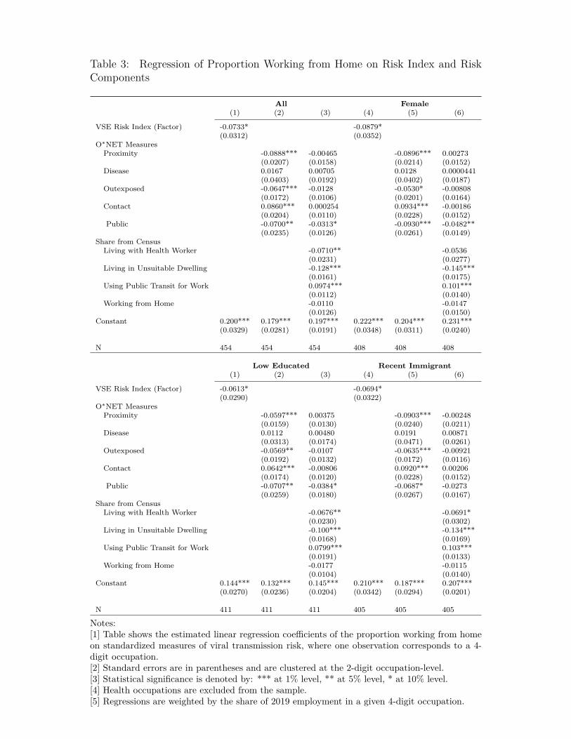
Table 3: Regression of Proportion Working from Home on Risk Index and RiskComponents

All Female

(1) (2) (3) (4) (5) (6)

VSE Risk Index (Factor) -0.0733* -0.0879*(0.0312) (0.0352)

OúNET MeasuresProximity -0.0888*** -0.00465 -0.0896*** 0.00273

(0.0207) (0.0158) (0.0214) (0.0152)Disease 0.0167 0.00705 0.0128 0.0000441

(0.0403) (0.0192) (0.0402) (0.0187)Outexposed -0.0647*** -0.0128 -0.0530* -0.00808

(0.0172) (0.0106) (0.0201) (0.0164)Contact 0.0860*** 0.000254 0.0934*** -0.00186

(0.0204) (0.0110) (0.0228) (0.0152)Public -0.0700** -0.0313* -0.0930*** -0.0482**

(0.0235) (0.0126) (0.0261) (0.0149)Share from Census

Living with Health Worker -0.0710** -0.0536(0.0231) (0.0277)

Living in Unsuitable Dwelling -0.128*** -0.145***(0.0161) (0.0175)

Using Public Transit for Work 0.0974*** 0.101***(0.0112) (0.0140)

Working from Home -0.0110 -0.0147(0.0126) (0.0150)

Constant 0.200*** 0.179*** 0.197*** 0.222*** 0.204*** 0.231***(0.0329) (0.0281) (0.0191) (0.0348) (0.0311) (0.0240)

N 454 454 454 408 408 408

Low Educated Recent Immigrant

(1) (2) (3) (4) (5) (6)

VSE Risk Index (Factor) -0.0613* -0.0694*(0.0290) (0.0322)

OúNET MeasuresProximity -0.0597*** 0.00375 -0.0903*** -0.00248

(0.0159) (0.0130) (0.0240) (0.0211)Disease 0.0112 0.00480 0.0191 0.00871

(0.0313) (0.0174) (0.0471) (0.0261)Outexposed -0.0569** -0.0107 -0.0635*** -0.00921

(0.0192) (0.0132) (0.0172) (0.0116)Contact 0.0642*** -0.00806 0.0920*** 0.00206

(0.0174) (0.0120) (0.0228) (0.0152)Public -0.0707** -0.0384* -0.0687* -0.0273

(0.0259) (0.0180) (0.0267) (0.0167)Share from Census

Living with Health Worker -0.0676** -0.0691*(0.0230) (0.0302)

Living in Unsuitable Dwelling -0.100*** -0.134***(0.0168) (0.0169)

Using Public Transit for Work 0.0799*** 0.103***(0.0191) (0.0133)

Working from Home -0.0177 -0.0115(0.0104) (0.0140)

Constant 0.144*** 0.132*** 0.145*** 0.210*** 0.187*** 0.207***(0.0270) (0.0236) (0.0204) (0.0342) (0.0294) (0.0201)

N 411 411 411 405 405 405

Notes:[1] Table shows the estimated linear regression coe�cients of the proportion working from homeon standardized measures of viral transmission risk, where one observation corresponds to a 4-digit occupation.[2] Standard errors are in parentheses and are clustered at the 2-digit occupation-level.[3] Statistical significance is denoted by: *** at 1% level, ** at 5% level, * at 10% level.[4] Health occupations are excluded from the sample.[5] Regressions are weighted by the share of 2019 employment in a given 4-digit occupation.

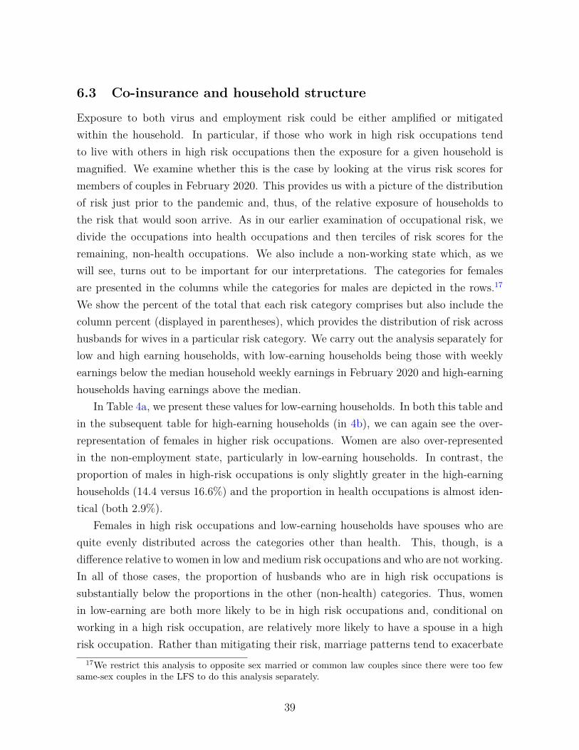
6.3 Co-insurance and household structure

Exposure to both virus and employment risk could be either amplified or mitigatedwithin the household. In particular, if those who work in high risk occupations tendto live with others in high risk occupations then the exposure for a given household ismagnified. We examine whether this is the case by looking at the virus risk scores formembers of couples in February 2020. This provides us with a picture of the distributionof risk just prior to the pandemic and, thus, of the relative exposure of households tothe risk that would soon arrive. As in our earlier examination of occupational risk, wedivide the occupations into health occupations and then terciles of risk scores for theremaining, non-health occupations. We also include a non-working state which, as wewill see, turns out to be important for our interpretations. The categories for femalesare presented in the columns while the categories for males are depicted in the rows.17

We show the percent of the total that each risk category comprises but also include thecolumn percent (displayed in parentheses), which provides the distribution of risk acrosshusbands for wives in a particular risk category. We carry out the analysis separately forlow and high earning households, with low-earning households being those with weeklyearnings below the median household weekly earnings in February 2020 and high-earninghouseholds having earnings above the median.

In Table 4a, we present these values for low-earning households. In both this table andin the subsequent table for high-earning households (in 4b), we can again see the over-representation of females in higher risk occupations. Women are also over-representedin the non-employment state, particularly in low-earning households. In contrast, theproportion of males in high-risk occupations is only slightly greater in the high-earninghouseholds (14.4 versus 16.6%) and the proportion in health occupations is almost iden-tical (both 2.9%).

Females in high risk occupations and low-earning households have spouses who arequite evenly distributed across the categories other than health. This, though, is adi�erence relative to women in low and medium risk occupations and who are not working.In all of those cases, the proportion of husbands who are in high risk occupations issubstantially below the proportions in the other (non-health) categories. Thus, womenin low-earning are both more likely to be in high risk occupations and, conditional onworking in a high risk occupation, are relatively more likely to have a spouse in a highrisk occupation. Rather than mitigating their risk, marriage patterns tend to exacerbate

17We restrict this analysis to opposite sex married or common law couples since there were too fewsame-sex couples in the LFS to do this analysis separately.

39

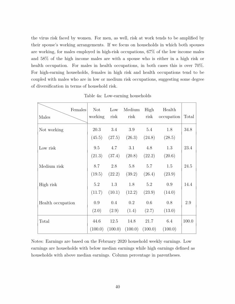
the virus risk faced by women. For men, as well, risk at work tends to be amplified bytheir spouse’s working arrangements. If we focus on households in which both spousesare working, for males employed in high-risk occupations, 67% of the low income malesand 58% of the high income males are with a spouse who is either in a high risk orhealth occupation. For males in health occupations, in both cases this is over 70%.For high-earning households, females in high risk and health occupations tend to becoupled with males who are in low or medium risk occupations, suggesting some degreeof diversification in terms of household risk.

Table 4a: Low-earning households

MalesFemales Not

workingLowrisk

Mediumrisk

Highrisk

Healthoccupation Total

Not working 20.3 3.4 3.9 5.4 1.8 34.8(45.5) (27.5) (26.3) (24.8) (28.5)

Low risk 9.5 4.7 3.1 4.8 1.3 23.4(21.3) (37.4) (20.8) (22.2) (20.6)

Medium risk 8.7 2.8 5.8 5.7 1.5 24.5(19.5) (22.2) (39.2) (26.4) (23.9)

High risk 5.2 1.3 1.8 5.2 0.9 14.4(11.7) (10.1) (12.2) (23.9) (14.0)

Health occupation 0.9 0.4 0.2 0.6 0.8 2.9(2.0) (2.9) (1.4) (2.7) (13.0)

Total 44.6 12.5 14.8 21.7 6.4 100.0(100.0) (100.0) (100.0) (100.0) (100.0)

Notes: Earnings are based on the February 2020 household weekly earnings. Lowearnings are households with below median earnings while high earnings defined ashouseholds with above median earnings. Column percentage in parentheses.

40

Table 4b: High-earning households

MalesFemales Not

workingLowrisk

Mediumrisk

Highrisk

Healthoccupation Total

Not working 0.0 1.1 0.6 0.7 0.4 2.8(0.0) (4.1) (2.7) (2.4) (3.2)

Low risk 5.1 12.0 9.2 11.5 5.5 43.3(49.8) (46.6) (43.3) (39.5) (40.2)

Medium risk 3.6 8.9 8.0 9.7 4.2 34.4(35.0) (34.8) (37.6) (33.4) (30.8)

High risk 1.3 3.4 3.1 6.5 2.3 16.6(12.9) (13.1) (14.5) (22.4) (16.7)

Health occupation 0.2 0.4 0.4 0.7 1.3 2.9(2.4) (1.4) (1.8) (2.3) (9.1)

Total 10.2 25.7 21.2 29.1 13.8 100.0(100.0) (100.0) (100.0) (100.0) (100.0)

Notes: Earnings are based on the February 2020 household weekly earnings. Lowearnings are households with below median earnings while high earnings defined ashouseholds with above median earnings. Column percentage in parentheses.

In Figure 17, we examine risk sharing in terms of job loss for couples. Given that weare examining couples, we take a slightly di�erent approach than in the rest of the paper.We restrict analysis to the January and February 2020 rotation samples since we areable to obtain pre-COVID occupation and household earnings information; then, usingthe longitudinal component of the LFS, we follow these two cohorts from February toJune. We examine the employment outcomes in terms of occupational risk and householdearnings which we define based on the February 2020 values. We categorize low riskhouseholds as those for which neither spouse worked in a high risk or health occupationin February and a high risk household as those for which at least one person of thecouple worked in either a high risk or health occupation. We show the fraction of eachearning/risk category for which both are employed, the male is employed and the femaleis not employed, the female is employed and the male is not employed, or both are notemployed.

41

Our analysis of job loss in Section 4 revealed that workers in occupations with higherVSE Risk Index scores experienced greater job loss. Here, we find the same viral risk-job loss relationship based on the household analysis. While there is a sizeable declinebetween February and April in terms of households in which both spouses are employedfor all four risk-earnings groups, we find that household with at least one worker in anoccupation with a high VSE Risk Index score see a disproportionate decline. This is trueeven though we have included health occupations in this group and health care job losswas minimal. The fraction of high earning/high risk households in which both membersof the couple were employed declined from 94 percent in February to 72 percent in April,while the fraction for the low earning/high risk households declined from 64 to 46 percentover the same period. the low risk groups also experienced declines in the proportion ofcouples in which both were employed, but to a lesser degree.

We can get an assessment of within-family employment insurance by examining move-ments in the proportion of couples in which both were not employed. For low earninghouseholds of both risk levels, the decline in the proportion with both employed is al-most exactly mirrored by the proportion in which neither worked. In contrast, in thehigh earnings households, the movement in the proportion of couples in which both arenot working is minimal. That is, high earnings couples were able to continue with atleast one member of the couple in work while low earnings couples were not. Thus, tothe extent that low earnings are correlated with low education, the larger job losses forlower educated workers is amplified by their household matches. Lower educated (lowearning) workers are more likely to have a spouse who also loses a job. Thus, they notonly face greater job risk, they have lower intra-household insurance against that risk.

42

Figure 17: Employment Outcomes by Household Earnings and Viral Risk

��

��

)HEUXDU\

0DUFK $S

ULO0D\

-XQH

)HEUXDU\

0DUFK $S

ULO0D\

-XQH

/RZ�HDUQLQJV��/RZ�0HGLXP�ULVN /RZ�HDUQLQJV��+LJK�ULVN�+HDOWK�RFF�

+LJK�HDUQLQJV��/RZ�0HGLXP�ULVN +LJK�HDUQLQJV��+LJK�ULVN�+HDOWK�RFF�

%RWK�HPSOR\HG 0DOH�HPSOR\HG��IHPDOH�QRW�HPSOR\HG

%RWK�QRW�HPSOR\HG )HPDOH�HPSOR\HG��PDOH�QRW�HPSOR\HG

Notes: Sample restricted to the 2020 January and February rotations. Household earnings andindividual risk index/occupation determined in February 2020.

7 Conclusion

The COVID pandemic has revealed the important inequalities that exist between workersin terms of their exposure to disease and to job loss, as well as the relationship that existsbetween the two forms of risk. In this paper, we characterize the distribution of bothrisks, and how they interact di�erently for women, low-educated workers, and recentimmigrants.

At the onset of the pandemic, we worked closely with public health authorities in

43

British Columbia and Québec to develop a risk index that could be used to plan theeconomic response to the crisis, the VSE Risk Index. The creation of this index consti-tutes our first contribution. While others before us have recognized the importance ofjob characteristics, input from public health o�cials and access to highly disaggregateddata allowed us to incorporate worker characteristics into the measure and evaluationof risk. In this paper, we show that for certain groups, like immigrants, characterizingrisk only in terms of at-work characteristics risk misses out an important dimension ofviral risk. Furthermore, we find evidence that at-work risk components typically useduntil now may in part proxy for risk faced by workers through their living arrangements.This is an important policy consideration going forward, as much of the debate on viralcontainment has focused on the work place.

Our second contribution is to characterize how the viral and employment risk, as wellas the relationship between the two, vary across various subgroups. We find that the VSERisk Index is highly correlated with the proportion of women in an occupation, but bearsno systematic relationship with other occupation-level worker characteristics, such as theprevalence of low-education workers in an occupation. Women also experienced impor-tant employment losses through the pandemic, contrasting with typical male-dominatedemployment losses in recent recessions. In comparison, low-educated workers and immi-grants were hit most substantially by the “pandemic” recession, even though we find noevidence that occupations with higher proportions of either group were at greater risk ofviral contagion.

While health occupations were among the riskiest in terms of viral contagion, the na-ture of the crisis was such that they experienced the smallest employment losses. Amongnon-health occupations however, we find a strong and positive relationship between viralrisk and employment losses. At the peak of confinement, in April, high-risk occupationshad lost 26.5% of employment, compared to less than 10% in low-risk occupations. Fur-thermore, while low-risk occupations had fully recovered by June, high-risk occupationswere still 15.5% below the February employment levels. In great part, the net e�ect ofthe pandemic on employment, with respect to risk, can be explained by the fact thathigh-risk occupations were more likely to lose employment, but no more likely to regainemployment after April. We show that the correlation between viral risk and employmentloss was largely driven by occupations in which workers are required to perform job tasksin close physical proximity to others. However, this factor itself appears to proxy at leastin part for economic disadvantage. Indeed, in regressions of occupation-level employmentloss on at-work and at-home risk components, we find that controlling for the share of

44

workers who live in crowded dwellings substantially reduces the size of the coe�cient onproximity.

Thus, both types of risk that we examine - risk of exposure to the virus and riskof job loss - increased in ways that reflect deep-seated inequalities in Canadian society.Women have faced greater virus risk exposure because of the occupations in which theytend to work. That greater risk exposure combined with the fact that high risk occu-pations were more likely to lose employment completely explains the higher job loss forwomen, especially when measured relative to earlier recessions. Moreover, they had lowerprobabilities than men of being employed but absent from work, i.e., to maintaining aconnection to the firm that turned out to improve workers’ abilities to reconnect withemployment during the recovery phase. They were also more likely than men to shiftto working from home, which is likely reflects their making sacrifices related to work inorder to care for children at home. At the same time, women did not face higher ratesof layo� within occupations of a given risk type. That is, women were not more likely tobe laid o� simply because they were women.

In contrast, low educated workers did not face higher exposure to virus risk on thejob but were much more likely to be laid o� than high educated workers. This fits withobservations in previous recessions that the low educated bear the brunt of job loss. Wepresent a rough counterfactual exercise that implies that in the Covid recession, the extrajob loss for the low educated can be accounted for by their lower propensity to switch toworking from home and that lower propensity is due not to their job characteristics butto their home characteristics such as their greater tendency to work in crowded dwellings.In essence, long standing inequalities in living arrangements interacted with the virus toyield inequalities in job loss.

Taken together, our results reveal the ways in which the Covid crisis exposed thedeep inequities in our society. Women faced more virus risk and were given less accessto ongoing connections to the firm because of long standing occupational patterns andthe division of work within the home. Low educated workers faced employment lossesbecause their living arrangements made it less possible for them to adjust to the labourdemand shock induced as a necessary response to Covid. The virus may a�ect us all butit moves through existing structures to increase inequality.

45

References

Cherno�, A. W. and C. Warman (2020, July). COVID-19 and Implications for Automa-tion. NBER Working Papers 27249, National Bureau of Economic Research, Inc.

Cortes, G. M. and E. Forsythe (2020, May). The heterogeneous labor market impacts ofthe COVID-19 pandemic. Working paper.

Dingel, J. I. and B. Neiman (2020). How many jobs can be done at home? Journal of

Public Economics 189, 104235.

Gamio, L. (2020, March 15). The workers who face the greatest Coronavirus risk. The

New York Times, https://nyti.ms/33j5mwB.

Jaimovich, N. and H. E. Siu (2020). Job polarization and jobless recoveries. Review of

Economics and Statistics 102 (1), 129–147.

Jones, S. R., F. Lange, W. C. Riddell, and C. Warman (2020). Waiting for recovery: TheCanadian labour market in June 2020. Canadian Public Policy 46 (S2), S102–S118.

Jones, S. R. and W. C. Riddell (2006). Unemployment and nonemployment: Hetero-geneities in labor market states. Review of Economics and Statistics 88 (2), 314–323.

Lemieux, T., K. Milligan, T. Schirle, and M. Skuterud (2020). Initial impacts of theCOVID-19 pandemic on the Canadian labour market. Canadian Public Policy 46 (S1),S55–S65.

Mongey, S., L. Pilossoph, and A. Weinberg (2020, April). Which workers bear the burdenof social distancing policies? BFI Working Paper No. 2020-51.

Mongey, S. and A. Weinberg (2020, March). Characteristics of workers in low work-from-home and high personal-proximity occupations. BFI White Paper.

Montenovo, L., X. Jiang, F. L. Rojas, I. M. Schmutte, K. I. Simon, B. A. Weinberg,and C. Wing (2020, May). Determinants of disparities in Covid-19 job losses. NBERWorking Paper No. 27132.

Vu, V. and N. Malli (2020, April 3). Anything but static: Risks of COVID-19 to workersin Canada. https://brookfieldinstitute.ca/p/7991.

46

NBER WORKING PAPER SERIES THE DISTRIBUTION OF COVID-19 ...

Documents

Transcript of NBER WORKING PAPER SERIES THE DISTRIBUTION OF COVID-19 ...