NBER WORKING PAPER SERIES

THE 1920s AND THE 1990s IN MUTUAL REFLECTION

Robert J. Gordon

Working Paper 11778http://www.nber.org/papers/w11778

NATIONAL BUREAU OF ECONOMIC RESEARCH1050 Massachusetts Avenue

Cambridge, MA 02138November 2005

This research has been supported by the National Science Foundation. I am grateful to Ian Dew-Becker forexcellent research assistance, to conference participants, Barry Eichengreen, and especially to Paul Davidfor thoughtful comments on the conference draft of this paper, and to my late father R. A. Gordon for askingtantalizing questions about the 1920s that, to this date, have not been satisfactorily resolved. The viewsexpressed herein are those of the author(s) and do not necessarily reflect the views of the National Bureauof Economic Research.

©2005 by Robert J. Gordon. All rights reserved. Short sections of text, not to exceed two paragraphs, maybe quoted without explicit permission provided that full credit, including © notice, is given to the source.

The 1920s and the 1990s in Mutual ReflectionRobert J. GordonNBER Working Paper No. 11778November 2005JEL No. E0, E21, E22, E32, N00, N12

ABSTRACT

This paper develops a new analysis of the U. S. economy in the 1920s that is illuminated bycontrasts with the 1990s, and it also re-examines the causes of the Great Depression. In both the1920s and the 1990s the acceleration of productivity growth linked to the delayed effects ofpreviously invented "general purpose technologies" stimulated an increase in fixed investment thatbecame excessive and proved to be unsustainable, while the productivity acceleration helps toaccount for low inflation in both decades. The uncanny parallel of the stock market boom, bubble,and collapse in 1995-2001 as in 1924-1930, reminds us that business cycles emerge from thecomplex interplay of multiple factors, not just one.

Common elements between the two decades are overshadowed by differences, including themuch larger share of agricultural output in the 1920s, the weakness of farm prices throughout thedecade, and the role of collapsing farm prices in the pervasive post-1929 downward shift inaggregate demand. Another partly related difference was a high volatility of inventory accumulationthat reflected the larger share of agriculture and manufacturing in the economy of the 1920s. Failuresof public policy in the 1920s included the absence of deposit insurance, the unit-banking regulationsthat prevented the diversification of financial risk across regions, and the low margin requirementsthat exacerbated swings in stock market prices. Further, the 1920s witnessed the advent ofprotectionism and the sharp curtailment of immigration.

The stability of the American economy after the 2000-01 collapse of investment and the stockmarket proves that good public policy matters, going beyond the narrowly defined operations ofmonetary and fiscal policy. Such highly diverse policies as banking regulation, deposit insurance,margin rules, reduction of tariffs, and loose restrictions on immigration all combine to make today'sAmerican economy more stable and less fragile than in the 1920s.

Robert J. GordonDepartment of EconomicsNorthwestern UniversityEvanston, IL 60208-2600and NBERrjg@northwestern.edu

1920s vs. 1990s, Page 1

1. This epigraph describes the Great Depression in language modelled on Keegan’s (1989, p. 5)description of World War II as the “greatest event in human history.”

ʺThe Great Depression of 1929 to 1940 in the United States was the greatest event in the history of businesscycles. It devastated rich and poor alike. It destroyed wealth in the billions, tossed one-quarter of the 1929labor force onto the shoals of unemployment, evaporated the hopes and aspirations of millions, left a majorityof American families near destitutuion for a full decade in an event that was totally unnecessary, becauseproperly applied monetary and fiscal policy could have cured the recession in 1930-31, not a decade later in1941.ʺ1

I. Introduction

The similarities in American economic performance between the decades of the

1920s and 1990s are tantalizing. Particularly when 1919 is aligned with 1990 and 1929 is

aligned with 2000, the evolution of many key macro variables over the intervening decade

match remarkably closely. Growth in real GDP, real GDP per capita, employment, and

productivity were almost identical, the conventionally measured unemployment rate was

identical in 1928 and 1999, inflation was negligible (1920s) or low (1990s), and the late-1920s

stock market boom is the only such episode in the century that comes close to the stock

marketʹs ebullience in the late 1990s. Like the 1990s, the 1920s witnessed prosperity, a

productivity revival, low unemployment, and low inflation. Both decades featured an

explosion of applications of a fundamental ̋ General Purpose Technology,ʺ electricity and

the internal combustion engine in the 1920s and computer hardware, software, and

networking communications technology in the 1990s. Both decades appear to mock the

existence of a Phillips-curve tradeoff between inflation and unemployment.

1920s vs. 1990s, Page 2

2. "Standard" discussions of the causes of the Great Depression include, among many, Eichengreen(1992b, 2000), Friedman and Schwartz (1963), and Temin (1976, 2000). Non-standard sources revived hereinclude R. A. Gordon (1951, 1961, 1974), Gordon and Wilcox (1981), and Gordon and Veitch (1986).

Yet the evolution of the economy after 1929/2000 was entirely different, except for

a short-run mirror-image in the stock market collapse. Viewed in their antiseptic

blandness, the raw data portray an economy in 1929 poised for continuous expansion and

a leap forward in the American standard of living. Yet the four years after 1929 produced

an economic disaster without parallel before or since in economic history. This paper goes

beyond the superficial similarity of the 1920s and 1990s to search for worms in the apple

of the 1920s. While accepting the role of domestic monetary policy and international

monetary relations in explaining the magnitude of the 1929-33 collapse, we identify lesser-

known aspects of the 1920s that made the economy more vulnerable to bad policy than was

true of the economy of the late 1990s.2

The aim of this paper is to find interesting features and puzzles about the 1920s that

might be illuminated in contrast with the 1990s. The emphasis is on understanding what

happened between 1919 and the summer of 1929, and there is no attempt here to revisit the

well-trodden turf of the disastrous conduct of the Federal Reserve after the stock market

crash, or the well-known set of factors that caused the Great Depression to be so deep, e.g.,

the relative roles of the Fed and the gold standard, bank failures and the absence of bank

deposit insurance, the Smoot-Hawley Tariff, or the British abandonment of the ʺgold

1920s vs. 1990s, Page 3

standardʺ in September, 1931. Instead, we focus on similarities and differences between

the 1920s and 1990s pertaining to the economy prior to 1930. The 1920s and 1990s shared

a common success, a distinct acceleration of productivity growth in comparison with the

previous two decades. The 1920s and 1990s shared common failurs, especially

overinvestment and the stock market bubbles. The 1990s illuminate the 1920s especially

in the demonstration that aggressive monetary and fiscal expansion limited the 2001

recession to the shallowest drop in real GDP in the postwar era, leading to the presumption

that similar policies could have had similar effects in 1930-31.

The pivotal role of information and communication technology (ICT) investment in

the boom of the late 1990s leads us to place our major emphasis on a reexamination of

investment in the 1920s. Was there “overinvestment” in equipment or structures in the

1920s by comparison with other decades in the twentieth century? We integrate the

previously diffuse literature on a business cycle interpretation of investment in the 1920s

with the productivity-based literature on general purpose technology (GPT) in the 1920s,

always placing the 1920s in the perspective of the same variables for the 1990s.

II. The Aligned Data on the 1920s vs. the 1990s

1. Growth Rates. Our comparison of data on the 1920s and 1990s begins with Table 1,

which displays annualized growth rates of numerous macro variables for the two decades, 1990-

1920s vs. 1990s, Page 4

2000 vs. 1919-29, and also breaks down the 1920s into its quite different sub-intervals of 1919-23 and

1923-29. Subsequently we will look at the levels (as contrasted to growth rates) of selected

indicators.

Our primary focus in Table 1 is on the first two columns, comparing 1990-2000 with 1919-29.

Here we find that real variables share growth rates that are amazingly similar while nominal

variables grow at slower rates in the 1920s, reflecting the complete absence of inflation in that

decade. Among the variables that grow at essentially the same rate in the 1990s as in the 1920s are

real GDP (line 2), nonfarm private business output, hours, and output per hour (lines 5-7), and the

nominal money supply (line 18). Hours per employee (line 8) were stable in the 1990s, in contrast

to a steady rate of decline in the 1920s that continued the long-term reduction in nonfarm private

hours per employee from 60 per week in 1889 to 40 per week in 1957 (Kendrick, 1961, Table A-IX,

p. 310).

However similar are the growth rates in the second section for the nonfarm private business

sector, the 1920s exhibit a clear superiority in productivity growth within the manufacturing sector.

While productivity growth in manufacturing was impressive in the 1990s, the performance of the

1920s was even better, particularly the great leap forward in manufacturing productivity achieved

between 1919 and 1923. The overall growth rate of manufacturing productivity of 5.4 percent per

year during the 1920s (Table 1, line 9) was more than quadruple the pathetic rate of 1.3 percent per

year registered in the previous three decades (1889-1919), supporting Paul Davidʹs oft-discussed

ʺdelayʺ hypothesis (1990, 1991), further developed in David-Wright (2000), that there was a long

1920s vs. 1990s, Page 5

3. The David-Wright (2000, pp. 6, 10) version recognizes the Henry Ford assembly line innovationand treats it as complementary to the electrification of manufacturing, and also related to the change in labormarket relations. These topics are treated further below.

delay in achieving the productivity payoff in manufacturing of the invention of electric power in

the 1870s. Clearly there was more going on in the 1920s than bringing electric motors to the

individual work station, and Henry Fordʹs invention of the assembly line in the preceding decade

deserves credit as well.3

Since inflation was zero in the 1920s as contrasted with a modest 2 to 3 percent in the 1990s

(lines 3 and 4), all nominal growth rates in the 1920s were substantially lower, including nominal

GDP (line 1), components of national income (lines 10 through 14), and the velocity of M2 (line 19).

One conspicuous exception is interest income, which grew more rapidly in the 1920s despite the

absence of any significant changes in interest rates during that decade. Employment and the labor

force grew more rapidly in the 1920s than in the 1990s, reflecting a growth rate of the working age

population that was more than twice as fast (line 17).

Perhaps the most intriguing similarity of the two decades was the run-up in stock market

prices towards the end of each period, see line 20. For the two decades as a whole, stock price

appreciation in the 1920s was much slower (9.9 percent) than in the 1990s (14.5 percent). This

reflects in part the absence of any increase at all in stock prices between 1919 and 1923. If we chop

off the first four years of each decade, then the increase in stock prices between 1923 and 1929 (17.0

percent per annum) is remarkably similar to that between 1994 and 2000 (18.9 percent per annum).

In fact, in real terms (deflating by the GDP deflator), the late-decade run-ups are almost identical,

1920s vs. 1990s, Page 6

17.0 percent for 1923-29 and 16.9 percent for 1994-2000.

2. A Long-run Comparison of Levels and Ratios. Some macroeconomic issues are

addressed by growth rates, as in Table 1. Others are better illuminated by raw numbers and ratios.

The top section of Table 2 provides the values of nominal and real GDP, the GDP deflator, and the

CPI for the beginning and end years of the 1920s and 1990s. Here we are impressed at how much

everything grew between 1929 and 1990, with compound annual growth rates of 6.6 percent for

nominal GDP, 3.5 percent for real GDP, and 3.1 and 3.3 percent, respectively, for the two inflation

measures. Compared to the six decades between 1929 and 1990, the decade of the 1990s exhibited

slightly slower real GDP growth and inflation, while the 1920s exhibited the same real GDP growth

with zero inflation.

The next section of Table 2 displays data on labor market outcomes. Of most interest is the

unemployment rate, which was lower in both 1919 and 1929 than in any year of the 1990s. The

labor-force participation rate was substantially higher in the 1990s than the 1920s, reflecting the

flow of women into the labor force that occurred during the postwar era. A crude measure of

productivity, real GDP per employee, grew by almost a factor of five between 1919 and 2000. But

its growth rates in the 1920s (1.8 percent per annum) and 1990s (1.9 percent) were not faster at all

than in the intervening decades 1929-90 (1.9 percent), perhaps a surprising result in view of the

common impression that productivity growth was particularly strong in the 1920s and 1990s.

The next section of Table 2 displays interest rates and a stock market index. It is perhaps

surprising to find that the nominal Treasury bill rate was lower in 1929 than in 2000. This

1920s vs. 1990s, Page 7

4. To calculate the real interest rate, I use the realized zero inflation rate of the 1920s for both 1919and 1929, the realized 1985-1990 3.2 percent average annual rate of increase in the GDP deflator for 1990,and the realized 1995-2000 increase of 1.7 percent for 2000.

difference is more than explained by different inflation rates, and the real interest rate in 2000 was

almost identical to that in 1929 and 1990.4 Clearly, the respect in which the 1920s and 1990s differed

most from the intervening decades (1929-90) was in the behavior of the stock market. The increase

in the S&P 500 stock market index, expressed in real terms, adjusting for the actual change in the

GDP deflator, was a soaring 11.3 percent per year in the 1920s and 12.4 percent in the 1990s,

dwarfing the puny 1.0 percent annual realized real return during 1929-90.

In addition to their distinction in the decadal league tables of stock market returns, the

decades of the 1920s and 1990s are perhaps best known for the diffusion of new technologies.

While the internal combustion engine and electric power generation had been invented in the 1870s

and 1880s, the 1920s represented a true breakthrough. Motor vehicle registrations more than

tripled between 1919 and 1929, and electricity generation more than doubled. In the 1990s the

number of Americans who reported using personal computers at home and/or at work more than

doubled, growing at roughly the same rate as electricity generation in the 1920s.

3. Charts. In this section we choose to display the aligned data over a longer period,

comparing 1913-32 with 1984-2003. The longer data period allows us to remain aware not only of

how much the evolution of the economy differed in 2000-2003 from 1929-32, but also how much

more volatile was the economy in the last years of World War I (1917-18) and in the period of

speculative boom and depression (1919-21), than in the aligned years 1988-2002.

1920s vs. 1990s, Page 8

With the 1913:1984 to 1932:2003 alignment, Figure 1 displays the astonishing similarity of

real GDP growth in the 1920s and 1990s. With a base year of 1929=2000=100, we note that the

growth rate of real GDP was identical over the intervals 1913-29 and 1984-2000, or alternatively

between 1919-29 and 1990-2000. However, much greater cyclical volatility of the earlier period

stands out in the chart. Taking the ratio of the 1913-32 index number for real GDP to the 1984-2003

number (as plotted in Figure 1), there was an additional GDP gap in 1914 compared to 1985 of -8.0

percent, in 1921 compared to 1992 of -9.7 percent, and in 1932 compared to 2003 of a gigantic -29.7

percent. The boom of the mid-1920s also outpaced the mid-1990s, with ratios of the real GDP

index in 1923, 1924, and 1926 to the corresponding years of the 1990s of +3.3 to +3.5 percent. While

Christina Romer (1989) has suggested that the standard data overstate the volatility of the pre-1929

economy relative to the post-1947 economy, from our narrower perspective there seems little doubt

that the macroeconomic environment was far more volatile during 1913-23 than in 1984-1994, the

“aligned” equivalent period.

Figure 2 shows that productivity growth in 1919-29 was identical to 1990-2000. However,

the two halves of the decade appear to have the reverse timing, displaying a slowdown in the 1920s

vs. an acceleration in the 1990s. Productivity growth in the 1920s slowed from annual rates of 2.7

percent in 1919-24 to 1.5 percent in 1924-29. In the 1990s the half-decades exhibited the exact

reverse behavior, with an acceleration from 1.6 percent in 1990-95 to 2.4 percent in 1995-2000. The

two eras also differed in that productivity growth was much faster during 1913-19 than in the

aligned years 1984-90, with respective annual growth rates of 2.2 and 1.5 percent.

1920s vs. 1990s, Page 9

5. Also, since a much larger share of the population was involved in the agricultural sector in the1920s than the 1990s, the unemployment statistics based on the nonagricultural sector bias downwards thevolatility of unemployment for the total economy in the 1920s compared to the 1990s.

The Lebergott (1964) unemployment data used by most economists are much more volatile

between 1913 and 1929 than in the recent period, as shown in Figure 3. Excluding the wartime

effect of 1918-19, the peacetime range was between 1.8 percent (1926) and and 11.7 percent (1921).

The equivalent range over the 1984-2003 interval was between 4.0 percent (2000) and 7.5 percent

(1984 and 1992). We should qualify the comparison in Figure 3 by noting that Lebergott does not

allow for cyclical variability of the labor-force participation rate. Thus he includes what we now

call “discouraged workers” as part of unemployment, whereas in the postwar BLS data they are

allowed to drop out of the labor force and are not counted as unemployed. This imparts a modest

excess volatility to the pre-1929 Lebergott unemployment data.5

Excess volatility is also displayed in Figure 4 by the inflation rate, with the CPI rising at an

annual rate of 14.7 in 1919-20 and declining at a rate of -11.3 percent in 1920-21. Yet, as shown

Tables 1 and 2 above, the price level was almost identical in 1919 and 1929, and the annual rate of

inflation between 1922 and 1929 was a mere 0.5 percent.

The final graphical comparison in Figure 5 displays the S&P 500 Stock Market Index. The

eight-year rise to the peak starting in 1921 and 1992 is absolutely identical, as is the four-year rise

to the peak starating in 1925 and 1996. The pattern of advance is slightly different, with a late surge

of 24 percent per year in the last two years of the 1920s episode (1927-29), wheres in the 1990s the

maximum growth in any year occurred earlier (26 percent in 1996-97). The comparison in Figure

1920s vs. 1990s, Page 10

5 somewhat overstates the similarity of the 1920s and 1990s, due to the absence of inflation in the

earlier decade. The overall increase in the stock market index when deflated by the GDP deflator

is 258 percent in 1921-29 compared to 197 percent in 1992-2000.

III. GPTs and the Productivity Growth Acceleration of the 1920s

The 1920s are a Janus-faced decade that defies simple characterization. At one level,

it was a quintessential decade of success, as was the 1990s. The 1920s were a golden age

of productivity growth (Kendrick, 1961; David-Wright, 2000), as were the 1990s (Jorgenson-

Stiroh, 2000, and Oliner-Sichel, 2002). Productivity growth accelerated after decades of

dismal quiesence, productivity growth in manufacturing outpaced the average of the

private nonfarm economy, inflation was low, monetary policy adopted benign neglect, and

in the golden spring of the terminal year of the decade of success, that is, the springs of 1929

and 2000, all was rosy and nothing could go wrong.

Yet the two decades ended very differently, the 1990s with a short, mild, recession

that brought with it an explosion in productivity growth, albeit a jobless recovery, while the

1920s ended with the catastrophe that has perplexed macroeconomists ever since. Our task

in this paper is to go beyond the well-worn explanation that monetary policy failed in 1929-

32. Yes, but why was monetary policy called upon to do anything? Why was there

anything to react against? Was there one or more “rotten apples” in the 1920s that explains

1920s vs. 1990s, Page 11

the economy’s post-1929 hangover, one with which monetary policy was not prepared to

deal?

The Janus-faced 1920s call for a multi-part analysis. Three previously unrelated sets

of literature require an attempt at a logical integration. First is the analysis of the

productivity growth acceleration of the 1920s, which carried on to the mid-1960s and was

the underlying source of the investment boom of the 1920s (David-Wright, 2000, R. J.

Gordon, 2000a). The second strand is the traditional set of business cycle models based on

the multiplier and accelerator; this treats every investment boom as inherently temporary

and carrying with it the seeds of its own destruction (Schumpeter, 1939; Samuelson, 1940;

Hicks, 1950; R. A. Gordon, 1951). Excess investment was the key ingredient that brought

the 1920s boom to an end and condemned the economy to a significant downturn, with an

effect that was significantly magnified by the stock market bubble. The third strand is best

known, the analysis of the domestic banking crisis and monetary policy failure associated

with Friedman and Schwartz (1963) and the complementary analysis of the international

monetary collapse furthest developed by Eichengreen (1992a, 1992b). Logic calls for these

three stands to be discussed in this order. Along the way, we will identify numerous

similarities between the 1920s and 1990s involving innovation, productivity growth, an

unsustainable investment boom, and a stock market bubble, and extreme differences

involving banking and monetary policy.

1920s vs. 1990s, Page 12

The Productivity Growth Acceleration and its Interpretation

The fundamental similarity between the 1920s and 1990s was identified by Paul

David (1990, 1991) before the 1990s had even begun! In his perceptive likening of the

computer to the “dynamo,” he developed what others have labelled the David “delay

hypothesis.” This was originally proposed as an explanation of the co-existence in the 1970s

and 1980s of slow productivity growth together with the spread of computers, a puzzle that

by then had become known as the Solow “computer paradox” – that “we can see the

computer age everywhere but in the productivity statistics.” In David’s analogy, the

invention of electricity and the electric power generation station in the 1870s and early 1880s

required decades of development and cost reduction before the full implications for

productivity and efficiency could be brought to fruition, and this occurred in the 1920s

when productivity growth accelerated, especially in manufacturing.

Subsequent to the initial David contribution, Bresnahan and Trajtenberg (1995)

popularized the term “general purpose technologies” (GPTs) for technical advances with

wide applications throughout the economy. The steam engine was the original GPT, but

doubtless the most important in history were the core inventions of the “Second Industrial

Revolution” of 1870-1900, electricity and the internal combustion engine. Gordon (2000b)

has questioned whether the chief GPT innovations of the late 1990s, the web and internet,

“measure up” to the pivotal inventions of the Second Industrial Revolution, electricity and

1920s vs. 1990s, Page 13

the internal combustion engine.

David (1990, 1991) identifies several factors which caused delay in the exploitation

of the potential of electric power and which finally released this potential after the period

1914-17, when there was a significant decline in the real price of electricity made possible

in part by a shift from isolated sources of electricity generation at individual industrial

plants to central station generating capacity. Continuous technological improvements in

central station generating equipment, together with a loosening of political regulation of

electric utilities, created the price decline that in turn “propelled the final phase of the shift

to electricity as a power source in U. S. manufacturing, from just over 50 percent in 1919 to

nearly 80 percent in 1929ʺ (David-Wright, 2000, p. 5). The technique for using electric

power also changed in the 1920s as well, from reliance on “group drives” to individually

powered machines, which then made possible a redesign of factories into single-story

factory layouts. This analysis of the sources of the 1920s productivity miracle in

manufacturing can be linked to the business-cycle literature on the 1920s investment boom,

which recognizes electrification as one source of the boom in both equipment investment

and commerical and industrial construction (see R. A. Gordon, 1974, p. 22).

For instance, the doubling of electricity output in the 1920s (Table 1 above) called for

significant investment in the utility industry. David-Wright (2000, pp. 6-7) call attention to

the effect of these developments in raising the productivity of capital, i.e., reducing the

1920s vs. 1990s, Page 14

6. A systematic feature of economic growth in the twentieth century was a steady rise in the ratio ofthe equipment capital stock to the structures capital stock, see Gordon (2000, Figure 2), where this isattributed to “space-saving innovation.”

capital-output ratio. R. J. Gordon (2000) notes the contribution of the increasing average

productivity of capital to the acceleration of multi-factor productivity growth that he dates

to the entire period between 1913 and 1964.6 Ironically, an increase in the productivity of

capital would tend to reduce the share of investment in real GDP and, after a transition

period of high investment in the 1920s, contributed to the weakness of investment in the

1930s. Both the 1920s and 1990s were characterized, at least after the fact, as periods of glut

and oversupply in capital equipment.

David-Wright (2000, pp. 23-26) emphasize the need for fundamental reorganizing

and rethinking of business practices in both the 1920s and 1990s. In this they anticipate the

recent literature on unmeasured “intangible investment” (business practice reinvention,

personnel training) that has been applied to the late 1990s productivity revival by Yang-

Brynjolffson (2001) and Basu et. al. (2003). David-Wright justify their emphasis on

electricity by noting that the productivity acceleration in manufacturing during the 1920s

was very widely dispersed across almost every sector of manufacturing, and they contrast

this “yeast-like” advance to the “mushroom-like” nature of productivity growth in the

1970s, 1980s, and 1990s, where productivity growth was much faster in some industries,

particularly in the manufacture of computers and semiconductors, than in others, e.g., most

1920s vs. 1990s, Page 15

7. David-Wright (2000, p. 10) treat the invention of the assembly line as one of three complementarycounterparts of electrification, but they make no comment on the role of the ICE in changing the location ofeconomic activity with the consequent implications for both productivity growth and investmentopportunities in the 1920s.

8. Production figures from R. A. Gordon (1974, p. 28). See also Historical Statistics series Q310 plusQ312. The ability of the American economy to produce 5.6 million internal combustion engines in 1929,about 80 percent of the world total, provides a central clue to the production miracle of America’s World WarII “arsenal of democracy.”

industries in nondurable manufacturing such as leather, tobacco, textiles, and apparel.

Qualifications

Two aspects of the David-Wright (2000) analysis require qualification, particularly

in looking for the sources of the investment boom of the 1920s and its subsequent collapse.

First, in their attention to the electrification of manufacturing, they fail to pay sufficient

attention to the effects of the other great GPT of the late nineteenth century, the internal

combustion engine (ICE), in generating investment in the 1920s. In part the role of the ICE

comes through a revolution in manufacturing technique parallel in importance to the

individual-drive electric motor, namely Henry Ford’s 1914 invention of the assembly line.7

Part of the productivity revolution in manufacturing in the 1920s came from the direct effect

of all the new factories and equipment needed to boost motor vehicle production from 1.9

million in 1919 to 5.6 million in 1929.8 Yet much of the influence of the ICE was outside of

manufacturing, with mobility made possible by the automobile and motor truck creating

entire new areas ripe for residential investment, and creating new opportunities to construct

facilities for wholesale and retail trade. Clearly the data of Table 1 above indicate that

1920s vs. 1990s, Page 16

productivity growth in the 1920s was less impressive outside of manufacturing than inside

that sector, but here we are interested not just in the role of the GPT innovations as a source

of productivity growth but also as a source of investment opportunities that fueled the

investment boom of the 1920s.

The David-Wright analysis, while lacking a sufficient emphasis on the role of the ICE,

joins together with electricity a second major source of the productivity acceleration of the

1920s, namely the “sharp increase in the relative price of labor” (David-Wright, 2000, p. 7).

The previous literature has not placed any significant emphasis on labor markets in

crediting the productivity acceleration or investment boom of the 1920s. Credit must be

given to the research of Goldin and Katz (1998) that emphasizes the uniquely American

development of secondary education, which spread high-school diplomas to most of the

population during the period between 1910 and 1940, and this must have had a payoff in

productivity growth in the decades after World War I.

But otherwise the David-Wright position does not accord with the facts. If there had

been a significant upward shift in the relative price of labor that was not justified by the

acceleration in productivity growth, then by definition labor’s share of national income

would have increased significantly. But as shown in Table 1, over the 1919-29 period

employee compensation rose at only 0.3 percent per year faster than national income, almost

the same as the 0.2 percent annual surplus registered in the 1990s. Doubt must be registered

1920s vs. 1990s, Page 17

about the factual accuracy of David-Wright’s claim (p. 7) that “the [real] hourly wage of

industrial labor was 50 to 70 percent higher after 1920 than it had been a decade earlier.”

Kendrick (1961, Table 26, p. 114) shows that the real price of labor per unit of labor (i.e., the

real wage) increased at only 1.4 percent per year during 1919-29, significantly slower than

the rate of 2.1 percent registered between 1899 and 1919.

IV. Investment in the 1920s: Boom and Collapse

The Keynesian tradition of business cycle theory associated with Samuelson (1939),

Hicks (1950), and many others identifies fluctuations in fixed investment, and to a lesser

extent consumer durables, as the primary impulse which drives the business cycle and

makes repeated but nonperiodic fluctuations inevitable. In Samuelson’s mathematically-

driven version (1939), the economy is condemned to explosive or damped cycles unless

parameters are at precise knife-edge values, leading postwar business cycle theorists to

deduce that the absence of damped or explosive cycles must imply a contribution of

irregular shocks outside the model. In Hicks’ (1950) version the evolution of output is

constrained by a capacity ceiling and floor based on the eventual need to replace

depreciating capital. Both of these models lack a government or foreign sector, nor do they

allow for any role of monetary or fiscal policy.

1920s vs. 1990s, Page 18

Investment in the 1920s and in the 1990s

This traditional Keynesian view traces the magnitude of the Great Depression back

to the investment boom of the 1920s. One way to assess the significance of the investment

boom is to compare the 1920s with the 1990s, when in the last part of the decade there was

a notable and unsustainable expansion of investment in producers’ equipment and

software. Our first comparison in Figure 6 shows the share in real GDP of spending on

Consumer durables plus all investment, including the change in inventories. The shares in

GDP are remarkably similar, peaking for the 1920s in 1925 with a GDP share of 27.1 percent

and peaking for the 1990s in 2000 with a share of 26.3 percent. The share in 1926 is almost

the same as in 1925, and in 1999 almost the same as in 2000.

But the yearly pattern is quite different. The investment share rose slowly and

steadily throughout the 1990s, whereas in the 1920s the share was quite volatile and peaked

four years before the end of the expansion. The shrinkage in the share from 27.1 percent in

1925 to 24.8 percent in 1929 suggests in the context of the multiplier-accelerator model that

weakness of fixed investment was already exerting downward pressure on aggregate

demand in 1929, temporarily masked by strength in consumption and inventory change.

The behavior of the investment-to-GDP ratio was totally different after the peak of the

expansion, declining only from 26.3 percent in 2000 to 23.9 percent in 2003, but from 24.8

in 1929 to a historically unprecedented 8.4 percent in 1932..

1920s vs. 1990s, Page 19

9. I confess guilt in this regard, as the author of a remark that I have often repeated, “In foursuccessive years (1924-27) the ratio of real residential construction to real GNP reached by far its highest levelof the twentieth century” (Gordon-Wilcox, 1981, p. 78).

The next three figures exhibit the decomposition of consumer durable spending and

total investment into five components. Shown in Figure 7 are the ratios for producers

durable equipment (including software in the 1990s) and consumer durables. Surprisingly,

the equipment boom of the 1920s is a pipsqueak, with a PDE share of about 5 percent,

compared to the 1990s when the share of PDE and software climbed from about 7 percent

in 1990 to about 9 percent in 2000. A second surprise is that, despite all of the consumer

durables for sale in the 1990s that had not yet been invented in the 1920s, the share of

consumer durable spending in the two decades is remarkably similar, tracking along in the

8 to 9 percent range during 1923-29 and 1994-2000. The sharp collapse after 1929 contrasts

sharply with 2000-03 when monetary ease buoyed sales of autos and other consumer

durables.

A further surprise is contained in Figure 8, which shows that residential structures

investment was not particularly high in the 1920s, with a peak ratio to GDP of 4.6 percent

in 2000, very close to the 1928 peak of 4.8 percent. Previous discussions implying an

unusually high residential investment ratio in the mid-1920s are simply incorrect and are

doubtless influenced by base-year relative price bias implied when residential construction

in the 1920s is restated at the high relative prices of the 1970s or 1980s.9 If anything in the

1920s vs. 1990s, Page 20

1920s was excessive, it was not residential investment but nonresidential investment, with

a peak ratio of 7.1 percent in 1925, drifting down to 5.5 percent in 1929, and then collapsing

to 2.4 percent. In the more recent decade the same ratio was 3.5 percent in 1990 and 3.2

percent in 2000. Taken together, the total share of residential and nonresidential structures

investment peaked at 11.4 percent in 1926 and by 1929 had declined to 9.1 percent, before

collapsing to 3.7 percent in 1932.

Perhaps the greatest difference between the 1920s and 1990s is in the time path of

inventory investment, a small and steady as a ratio to GDP in the 1990s, as shown in Figure

9, but large and volatile in the 1920s, with GDP ratios ranging between +5.5 percent in 1920

and -1.0 percent in 1924. Inventory investment contributed significantly to the Great

Contraction, with a collapse in the GDP ratio from +1.5 percent in 1929 to -4.0 percent in

1932. The behavior of inventory investment in the 1990s could not have been more

different, with a range during the 1990s only between 0.0 percent in 1991 to a maximum of

0.9 percent in 1994 and 1997, and with a decline in the recession year 2001 only to -0.4

percent.

The Interpretation of Investment Behavior in the 1920s

One reaction to the display of the investment ratios in Figures 6-9 might be “so

what?” The share of all components of spending must sum to 100 percent, so why does it

matter whether the investment ratio rises or falls? The significance of the ratio requires a

1920s vs. 1990s, Page 21

Keynesian (or IS-LM) interpretation in which economic fluctuations are driven by shifts in

“autonomous spending,” whether investment, government spending, exports, or the

autonomous component of consumption. The rest of spending, consumption of

nondurables and services, is passive, responding through the consumption function and the

multiplier to the autonomous demand shifts. This framework is entirely compatible with

a parallel emphasis on the role of monetary and fiscal policy. Monetary policy enters as a

driver of consumer durables and investment spending, while fiscal policy enters as a source

of autonomous spending shifts, and through the effect of tax changes in shifting the

consumption function.

Why was there an investment boom in the 1920s, and which factors apply to the

1990s as well? R. A. Gordon (1974, p. 27) lists seven factors that caused the high level of

investment in the 1920s: (1) “pent-up demand” created by the diversion of resources to

military spending during World War I; (2) direct and indirect effects of the automobile, (3)

demands related to other new industries including electric power, electrical equipment,

radio, telephone, air transport, motion pictures, and rayon; (4) rapid pace of technological

change and resulting rise in productivity, (5) rise to the peak in a long building cycle, (6) a

“wave of optimism,” and (7) elastic credit supply. Factors (3) and (4) are compatible with

the David-Wright (2000) emphasis on electricity and the productivity acceleration, while

factor (2) is consistent with our emphasis above on the ICE as an additional GPT in addition

1920s vs. 1990s, Page 22

10. See Hickman (1974, Table 3, p. 307) and Gordon-Wilcox (1981, footnote 34, p. 103) whoprovide a detailed interpretation of Hickman’s simulations. Interestingly, the ratios to GDP in Gordon-Wilcox (Table 6) are almost double those in Figure 8 above, suggesting an important base-year relative pricebias in the data used by both Hickman and Gordon-Wilcox.

to electricity.

The traditional literature on investment in the 1920s (R. A. Gordon, 1951, and

Hickman, 1974) emphasizes factor (5), the “overbuilding” in residential construction, which

was in part due to the failure of market participants to work out the implications of slower

future population growth implied by restrictive immigration legislation of the early 1920s.

Hickman (1974) used a dynamic simulation to conclude that, sheerly on the basis of an

autonomous demographic shift, housing starts would have declined from 1925 to 1930, even

with no decline in income, by 49 percent.10 Nevertheless, in the context of Figure 8, this

earlier literature appears to overemphasize residential investment and underemphasize the

larger rise and subsequent collapse of nonresidential investment in structures.

Most of the factors on the R. A. Gordon list of seven can be applied as well to the

investment boom of the 1990s, except for the first, pent-up demand caused by a previous

war. The invention of the internet, web, and mobile telephone, and the spread of personal

computers, were the GPTs that drove the investment boom, especially during 1996-2000.

A “wave of optimism” repeated the timing of the 1920s stock market bubble with a nearly

perfect repetition of timing and magnitude, and credit was even easier, in the sense that

1920s vs. 1990s, Page 23

growth in the money supply did not repeat in 1999-2000 the deceleration of 1927-29.

A more sophisticated analysis of total investment in the 1920s, combining both

residential and nonresidential structures, is provided by Gordon-Veitch (1986, pp. 316-7).

They create a unique data base consisting of quarterly data for components of GDP

covering the interwar period (1919-41) and analyze these data using a VAR model

containing structures investment, equipment investment, noninvestment GDP (of which 85

percent is consumption), the real monetary base, the money multiplier, and the corporate

bond rate. They carry out exogeneity tests showing that structures investment is largely

exogenous, with modest feedback from noninvestment GNP. There is significant feedback

from the monetary variables to both equipment investment and noninvestment GDP. There

is strong feedback from the spending variables to the monetary variables, while the interest

rate is largely exogenous. They conclude that there were two impulse sources in the

interwar business cycle, one “financial” working through the interest rate and money

multiplier, and another “real” working mainly through investment in structures.

Innovation accounting with the same VAR model supports the view that “structures appear

to be virtually autonomous” (Gordon-Veitch, p. 315). In their words concerning the

behavior of structures investment:

There is a high plateau in the own innovations series in 1926-27, a gradualdownward movement in 1928-29, and a sharp plunge beginning in 1929:3,before the fourth-quarter stock market debacle. Equally interesting is that the

1920s vs. 1990s, Page 24

own innovation series remains negative throughout 1931-41, supporting theinterpretation of “overbuilding” in the 1920s that required a long period ofsubsequent adjustment in the 1930s (Gordon-Veitch, pp. 316-17).

The parallel VAR analysis of equipment investment in the interwar period reveals a much

smaller autonomous own-innovation for equipment investment than for structures, and

much more of a role for feedback from both non-investment GDP and the monetary base.

The VAR analysis allows an examination of the residuals from these equations, which

are the “own-innovations” in each variables. There were large negative innovations in

structures investment in 1929:3 and 1929:4, in equipment investment in 1929:4, and in the

monetary base in 1929:1. Large negative innovations also occur in non-investment GDP in

1931:3 and in the money multiplier in 1931:2, 1931:3, and 1931:4. Using these results,

Gordon and Veitch reassessed Temin’s (1976) well-known anti-monetarist position based

on an autonomous downward shift in the consumption function in 1930. Their results

appear to contradict the Temin hypothesis, and they state that “we find no evidence that

negative residuals for nondurables consumptiion played a key role in the initial stages of

the Great Contraction” (Gordon-Veitch, pp. 321-2). Their VAR models shows that the

cumulative residuals (i.e., the “own-shock”) to noninvestment GDP, which is almost entirely

consumption, in 1929-30 amounted to only -1.6 percent of its level in mid-1929. In contrast,

the cumulative quarterly residuals for structures investment cumulated in 1929-30 to -25.2

percent and for equipment investment to -17.2 percent of their 1929 levels.

1920s vs. 1990s, Page 25

While the Gordon-Veitch residuals cumulated for 1929-30 are not large, their own

results contain support for Temin in a pattern that they did not apparently notice. Their

results for nondurable consumption exhibit a sharp shift from a cumulative residual of +3.4

percent in the first three quarters of 1929 to a cumulative -4.5 percent in the subsequent five

quarters (Gordon-Veitch, 1986, Table 5.9, p. 321). Thus they are correct that the primary

deflationary demand impulse prior to the stock market crash was in investment, not

consumption, however, their results are also consistent with Temin’s emphasis on an

autonomous downward shift in consumption beginning with the market crash and

continuing through the end of 1930. Their results also support the monetarist position, in

that the cumulative own-residual for the monetary base in 1929-30 was -20.5 percent of the

1929 value. Thus there appears to be a great deal of support, using modern econometrics,

that the key downward demand shocks prior to the crash were to fixed investment and the

real monetary base, but that consumption contributed significantly to the propagation of the

contraction in 1930 and the money multiplier contributed in 1931-32.

V. Domestic and International Monetary Policy

The analysis of Friedman-Schwartz (1963) is so well known, and the critique of the

F-S analysis has also been so often discussed (Temin, 1976), that only a few brief comments

1920s vs. 1990s, Page 26

11. A contrarian claims that the Fed’s tightening in 1928-29 was minor, did not affect borrowing for“legitimate business purposes.” “The tightness in credit affected speculation, but this is another matter.” SeeR. A. Gordon (1961, p. 427).

are required here. The role of money can be divided up into three intervals, 1927-29, 1929-

31, and 1931-33. Regarding 1927-29, a consensus has emerged that “increasingly stringent

U. S. monetary policy contributed significantly to the onset of the slump” (Eichengreen

1992b, p. 221). The annual growth rates of both M1 and M2 slowed sharply from 1925 to

1927, and in the case of M1 were negative in both 1927 and 1928 before turning slightly

positive in 1929. Interest rates increased, although only modestly by the standards of

postwar monetary tightening. Gordon-Wilcox (1981, p. 66) used quarterly data to compute

that the growth rate of M2 slowed from 5.2 percent at an annual rate in the five quarters

ending in 1927:4 to only 0.6 percent in the seven quarters beginning in 1928:1. After

remaining at 4 percent or below from mid-1924 to January, 1928, the Fed’s rediscount rate

was raised in several steps from 3.5 percent in that month to 5 percent in July, 1928, and

then with one final increase to 6 percent in August, 1929.11

Tightening by the Fed helped to create the Great Depression because of the role of

U. S. foreign lending in recycling European balance of payments deficits, and because the

return of the gold standard forced countries to respond to a loss of gold by domestic

monetary tightening. The Fed’s tightening in the U. S. coincided with a stabilization of the

French franc. As described by Eichengreen:

1920s vs. 1990s, Page 27

12. U. S. exports were about 5 percent of GDP in 1929.

As the U. S. and France siphoned off gold and financial capital from the restof the world, foreign central banks were forced to raise their discount ratesand to restrict the provision of domestic credit in order to defend their goldparities. Superimposed upon already weak foreign balances of payments,these shifts in U. S. and French policy provoked a greatly magnified shift inmonetary policy in other countries (Eichengreen, 1992b, p. 221).

Eichengreen quantifies the restrictive impulse, showing that the annual growth rate of

monetary aggregates in Europe and Latin America fell in 1927-28 by 5 percent and by an

additional 5 percent in 1928-29.

After the 1929 stock market crash, there was a two-way transmission of negative

demand shocks between the U. S. and foreign countries. The restrictive foreign monetary

policies that had been partly caused by the Fed’s actions reduced U. S. exports.12 The stock

market crash itself depressed consumption, as emphasized by Temin (1976, 1990) and

supported by the results of Gordon-Veitch. Beginning in 1930 bank failures became a

separate source of deflationary pressure, and their effect worsened after Britain left the gold

standard and devalued the pound in September, 1931.

The 1970s and early 1980s were characterized by a debate involving Temin, Schwartz,

Darby, and others, about the causes of the Great Contraction, as to whether “only money

mattered” or “money didn’t matter at all.” The anti-monetarist camp led by Temin focussed

largely on the behavior of consumption and strangely neglected the more important

1920s vs. 1990s, Page 28

autonomous influence coming from fixed investment. But statistical results, including those

of Gordon-Veitch discussed above and related work by Gordon-Wilcox (1981) support a role

for both autonomous demand shocks and feedback from restrictive monetary policy.

Gordon-Wilcox conclude:

Though monetary growth decelerated in 1928 and 1929, such a monetaryslowdown had happened before and can only account for 18 percent of theobserved decline in nominal income in the first year of the contraction and 26percent cumualtively in the first two years. . . . both monetary andnonmonetary factors mattered, nonmonetary factors were of primeimportance in 1929-31, different monetary policies in the United States after1931 would have reduced the severity of the contraction (Gordon-Wilcox,1981, p. 67, 74).

Their comment about 1931-33 is supported by a comparison of the behavior of M2 and

nominal GDP in the U. S. with an aggregate of seven major Western European nations. Both

M2 and nominal GDP began to rise after 1931 in Europe, whereas both continued to decline

through 1933 in the U. S.

VI. Other Similarities and Differences between the 1920s and 1990s

Financial Speculation and Accounting Fraud

Not only were the decades of the 1920s and 1990s uncannily similar in the magnitude

and timing of the stock market boom and collapse in both decades, but also in the fragility

of the financial system. The stock market boom was sustained in 1999 and 2000 by an

1920s vs. 1990s, Page 29

13. A more detailed analysis of financial fragility in the 1920s is provided by White (2000, pp. 752-7).

overstatement of corporate profits subsequently revealed to involve corruption, cheating,

and accounting scandals that brought familiar televised scenes of corporate executives in

handcuffs and the collapse of one of the big-five auditing firms. A wave of mergers,

acquisitions, initial public offerings, and venture capital investments was part of the

speculative froth of financial markets in the late 1990s, followed by the bankruptcy of many

of the new “dot-coms” and equity price declines of 90 percent or more for the hi-tech

corporations that succeeded in avoiding bankruptcy.

Similarly, a major part of new equity issues in the late 1920s rested on a fragile base.

“The major part, particularly from 1926 on, seems to have gone into erecting a financial

superstructure of holding companies, investment trusts, and other forms of intercorporate

security holdings that was to come crashing down in the 1930s” (R. A. Gordon, 1974, p. 35).13

Also similar in the 1920s and 1990s were large profits by investment bankers and a stimulus

to consumer demand coming from capital gains on equities. Equity speculation, as in the

1990s, led to overinvestment in some types of equipment and structures in the 1920s, just

as the 1990s witnessed a glut of investment in fiber-optic cable, other telephone equipment,

and dot-com software. The glut of investment goods created during the 1920s were to

“hang over the market” for the entire decade of the 1930s.

1920s vs. 1990s, Page 30

The evolution of the economy after 2000 was, of course, entirely different than after

1929, and we have previously attributed this to the aggressive easing of monetary policy

that sustained a major boom in residential construction and in sales of consumer durables

sufficient largely to offset the decline of investment in equipment and software. A second

difference was the aggressive easing of fiscal policy in 2001-03 through a succession of

reductions in Federal income tax rates, including the tax rates on capital gains and

dividends. A third major difference was that equities could be margined up to 90 percent

in the late 1920s, compared to 50 percent in the 1990s, raising both the level of speculative

frenzy in 1927-29 and the extent of wealth destruction when the crash finally came.

An aspect of the 1920s that has no counterpart in the 1990s is the weakness of the

banking system, due in part to regulations that prevented banks in many states (like Illinois)

from establishing branches. In 1924 only eleven states allowed statewide branching (White,

2000, p. 749). Regulations set the stage for the banking collapse of 1930-31, as the

prohibition on branch banking created a system of thousands of individual banks with a

fragile dependence on the ups or downs of economic conditions in their local community,

often tied to particular forms of agriculture (White, 2000, p. 750).

Two other institutional aspects of the 1920s also differed from the 1990s. A glaring

difference is the absence of deposit insurance. When the banks failed beginning in 1930, the

lifetime savings of many American households evaporated, aggravating the decline in

1920s vs. 1990s, Page 31

aggregate demand. Second, the stock market boom and collapse was exacerbated by loose

margin requirements that allowed investors to borrow 90 percent of the value of stocks, in

contrast to the 50 percent rule in effect during the 1990s.

Weakness in Agriculture

One aspect of the 1920s emphasized by previous authors is the overexpansion of

agriculture during the boom days of 1919-20 when agricultural exports to destitute Europe

exploded, only to be followed by a collapse of agricultural incomes and prices after

European agricultural capacity recovered (see R. A. Gordon, 1974, pp. 36-37). Weakness in

agricultural prices helped to keep overall inflation low, in an era in which agriculture was

a much larger share of output and employment than in the 1990s. Thus the boom of the

1920s was largely an urban phenomenon, and the weakness of agricultural prices and

incomes lay the seeds for the role of the farm sector in the post-1929 collapse, exacerbated

by the worldwide decline in commodity prices.

Both R. A. Gordon and Olmstead and Rhode (2000, Figure 12.1, p. 701) emphasize

that agricultural productivity stagnated in the 1920s and took off after the mid-1930s as the

full mechanical revolution made possible by the tractor took place. Olmstead and Rhode

point to the penetration of motor vehicles on the American farm by 1929 (with a 1919-1929

increase from 48 to 78 percent, Figure 12.3, p. 712), but the much slower diffusion of

electricity into rural America. This reinforces our point made above that David-Wright

1920s vs. 1990s, Page 32

overstate the relative importance of electricity relative to the internal combustion engine in

the productivity achievement of the U. S. in the 1920s.

Wage Flexibility and the Phillips Curve in the 1920s and 1990s

One of the most intriguing similarities between the 1920s and 1990s is the coincidence

of relatively low unemployment in both decades with low inflation in the 1990s and zero

inflation in the 1920s. The reasons for low inflation in the 1990s are well understood. A

large literature, beginning with Staiger-Stock-Watson (1997) and Gordon (1997), identified

a decline in the natural rate of unemployment, or “NAIRU” (non-accelerating inflation rate

of unemployment). This decline, which allows the inflation rate to be stable at a lower rate

of unemployment, has been attributed to a demographic shift away from teenagers who

naturally tend to have higher unemployment rates, an improvement in the micro-efficiency

of labor markets made possible by temporary help agencies, and even the rise in the fraction

of young adults incarcerated in prisons, some of whom would have been otherwise

unemployed.

Beyond the decline in the NAIRU between 1985 and the late 1990s, Gordon (1998) has

drawn attention to supply shocks as explaining both the high inflation in the 1970s and low

inflation in the late 1990s. In both decades movements in exchange rates and import prices

pushed inflation up (1970s) or down (1990s). In both decades productivity growth was a

key explanatory factor, with the productivity growth slowdown of the 1970s pushing

1920s vs. 1990s, Page 33

inflation up and the productivity growth revival of the 1990s pushing inflation down.

Inflation was also held down in the late 1990s by a more rapid rate of decline in the prices

of computers and by a temporary hiatus in medical care deflation.

Inflation in the 1920s is more of a puzzle, because the overall price level was so

volatile in 1916-22 and so stable during 1922-29. Gordon (1982) interprets rapid price

adjustment in 1916-22 as an “abberration, reflecting the ability of economic agents to change

their price-setting practices when they are universally aware of a special event (wartime

government purchases and deficit spending) that has a common effect on costs and prices.”

He interprets the post-1922 behavior as a “return to normal” in which firms focussed on

microeconomic “industry-specific” disturbances to costs and prices that were now large

relative to any remaining macroeconomic disturbance.

It is still unclear from recent research how much the experience of the 1920s differed

from that prior to 1914. Eichengreen (1992b, p. 217) and David-Wright (2000, pp. 20-21)

emphasize the shift in the nature of U. S. labor markets from flexible casual labor markets

to those dominated by implicit contracts and a tradeoff between wages and skills. With the

rise of high school educational attainment (discussed above), firms now valued their most

highly skilled workers and were willing to pay them extra. In this era were planted the

seeds of the subsequent efficiency-wage model and also the seeds of nominal wage rigidity.

It is unclear how much the 1920s represented a new era in labor-management relations, and

1920s vs. 1990s, Page 34

14. R. A. Gordon (1961, pp. 357-58) briefly describes and dismisses “underconsumptionist” theoriesand in his final evaluation of the causes of the Great Contraction (1961, p. 445) ascribes much more credenceto overinvestment than underconsumption.

to what extent the stability of wages and prices represented a return to norms that prevailed

before 1914.

Overall, the low rate of inflation in the 1920s combined the weakness of farm prices,

the absence of labor unions, and the direct role of the acceleration of productivity growth

in holding down inflation. Our explanation of low inflation in the 1990s shares the element

of an acceleration of productivity growth, and the declining importance of labor unions in

the 1990s echoes the near-absence of unions in the 1920s.

The Income Distribution

To insert any discussion about the income distribution in a paper on the

macroeconomics of the 1920s and 1990s may seem arcane. But there is an old literature that,

looking for “rotten” aspects of the 1920s, found an inadequacy of real income among the

masses to be a source of subsequent “underconsumption.”14 We have already examined

evidence in Table 1 above regarding the evolution of labor’s share in national income and

have found that the growth in employee compensation during the 1920s was roughly the

same as national income.

But the functional distribution of income between labor and capital is not the only

dimension of the income distribution. The other dimension is vertical inequality as

1920s vs. 1990s, Page 35

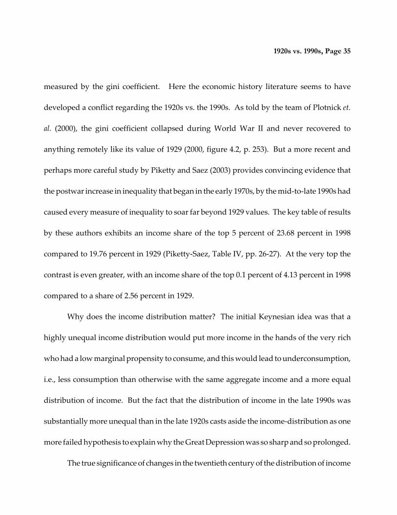
measured by the gini coefficient. Here the economic history literature seems to have

developed a conflict regarding the 1920s vs. the 1990s. As told by the team of Plotnick et.

al. (2000), the gini coefficient collapsed during World War II and never recovered to

anything remotely like its value of 1929 (2000, figure 4.2, p. 253). But a more recent and

perhaps more careful study by Piketty and Saez (2003) provides convincing evidence that

the postwar increase in inequality that began in the early 1970s, by the mid-to-late 1990s had

caused every measure of inequality to soar far beyond 1929 values. The key table of results

by these authors exhibits an income share of the top 5 percent of 23.68 percent in 1998

compared to 19.76 percent in 1929 (Piketty-Saez, Table IV, pp. 26-27). At the very top the

contrast is even greater, with an income share of the top 0.1 percent of 4.13 percent in 1998

compared to a share of 2.56 percent in 1929.

Why does the income distribution matter? The initial Keynesian idea was that a

highly unequal income distribution would put more income in the hands of the very rich

who had a low marginal propensity to consume, and this would lead to underconsumption,

i.e., less consumption than otherwise with the same aggregate income and a more equal

distribution of income. But the fact that the distribution of income in the late 1990s was

substantially more unequal than in the late 1920s casts aside the income-distribution as one

more failed hypothesis to explain why the Great Depression was so sharp and so prolonged.

The true significance of changes in the twentieth century of the distribution of income

1920s vs. 1990s, Page 36

lie elsewhere, not about the topic of aggregate demand and business cycles, but about the

time sequence of productivity growth in the twentieth century. The U-shaped evolution

of the income distribution, with inequality high before 1929 and in the late 1990s, is a

symptom of a set of causal factors that also mattered for productivity growth. Three

developments starting in the early 1920s served to make unskilled labor more expensive,

deliver a “rent” to high-school dropouts and graduates alike, and creating a strong incentive

to substitute capital for labor. These three were the New Deal legislation that legitimized

labor unions in the mid-1930s, the legislation that limited immigration beginning in the

early 1920s (together with the Great Depression and war that virtually eliminated

immigration), and the movement to high tariffs (Fordney-McCumber in 1922 and Smoot-

Hawley in 1930) together again with Depression and war that reduced imports to a

historical low percent of GDP. Supported by unions, and freed from competition from

unskilled immigrants and foreign unskilled labor embodied in imported goods, American

unskilled labor did exceptionally well from the mid-1930s to the late 1960s, and this comes

out as a sharp reduction in inequality between 1929 and 1945, followed by a plateau of low

inequality, and then a steady rise in inequality after 1970 climaxing in the late 1990s. Income

inequality is a symptom of other labor market developments, not a cause. Income

inequality was a symptom of the rents earned by low-skilled workers in what has been

called “The Great Compression” of the income distribution (Goldin-Margo, 1992).

1920s vs. 1990s, Page 37

VII. Conclusion

This paper has developed an analysis of the U. S. economy in the 1920s, newly

illuminated by the perspective of the economy of the 1990s. The centerpiece of our analysis

has been to integrate the previously unconnected contributions of David (1991) and David-

Wright (2000) on the productivity growth acceleration of the 1920s, with an earlier business

cycle literature associated with Schumpeter (1939), Samuelson (1940), and R. A. Gordon

(1951, 1974) that emphasizes the role of overinvestment in the 1920s as setting the stage for

the post-1929 collapse.

David (1991) creatively linked the disappointing productivity payoff from the

computer to the earlier history of electric motors and electricity generation. He found good

reasons why roughly 40 years evolved between the initial electric power station in 1882 and

the explosion of productivity growth in U. S. manufacturing in the 1920s, and reasoned that

a similar delay, for similar reasons, could be postponing the productivity payoff from the

electronic computer in the 1970s and 1980s. Anyone who predicts a phenomenon years

before its appearance deserves high praise, and David’s predicted productivity resurgence

in manufacturing and the broader economy occurred in the decade after 1995.

The electricity-computer analogy developed by David (1991) and further by David-

Wright (2000) sets the stage for the integration carried out in this paper. In both the 1920s

1920s vs. 1990s, Page 38

and the 1990s the acceleration of productivity growth linked to the delayed effects of

previously invented “general purpose technologies” stimulated an increase in fixed

investment that in both decades became excessive and proved to be unsustainable. The

1990s remind us that, even with better institutions, better information, and better policies,

it is possible for “overinvestment” to occur. In 2000-01 everything collapsed, including hi-

tech investment, the prices of hi-tech stocks, and many of the “New Economy” dot-com

startups failed. The uncanny parallel of the stock market boom, bubble, and collapse in

1995-2001 as in 1924-1930, with the side-by-side tale of emotional speculation, overheated

activity by investment bankers, and a parallel tale of pyramid building (in the 1920s) and

accounting fraud (in the late 1990s) reminds us that business cycles emerge from the

complex interplay of multiple factors, not just one. They are not just about monetary and

fiscal policy, but about powerful economic forces against which monetary and fiscal policy

can react or fail to react. Monetary policy responded in 2001-02 with a rapid decline in

interest rates, and fiscal policy responded with significant reductions in income tax rates.

Monetary policy failed to react in 1929-33 by allowing banks to fail and the money supply

to decline, and a perverse fiscal policy actually increased tax rates in 1932.

This paper integrates a previous literature claiming that one single factor or another

was “the primary cause” of the Great Depression. Econometric time-series analysis based

on quarterly data for the interwar period demonstrates that in 1928-29 the economy was

1920s vs. 1990s, Page 39

exposed to two major demand shocks, not just one. Negative shocks to investment demand

occurred prior to the 1929 stock market crash, and these combined with the negative

demand impulse of tighter monetary policy. These two negative shocks were joined after

the crash by a significant negative shock to consumption relative to income that persisted

through the end of 1930.

Going beyond the parallels between the 1920s and 1990s involving a productivity

growth acceleration and the accompanying booms of investment and the stock market, the

paper uncovers other similarities but also differences. The productivity growth

accelerations of the 1920s and 1990s both contribute to the explanation of why inflation was

so low in both decades. An additional explanation of low inflation is provided by the

absence of unions in the 1920s and their eroding presence in the 1990s. The accounting

scandals and froth of financial speculation of the late 1990s contributed to financial fragility

in a new but similar form to the financial superstructure of intercorporate security holdings

that developed in the late 1920s and came crashing down thereafter.

But the differences between the 1920s and 1990s also stand out, and these go beyond

the differing responses of monetary and fiscal policy to the collapse of investment and the

stock market. An important difference was the much larger share of agricultural output

and employment in the economy of the 1920s and the weakness of farm prices and incomes

throughout most of that decade. In this sense the boom of the 1920s was largely an urban

1920s vs. 1990s, Page 40

phenomenon that did not extend across the entire economy, and the post-1929 collapse in

commodity prices rippled through the farm sector and created an additional component to

the pervasive downward shift in aggregate demand. Another partly related difference was

the higher volatility of macroeconomic indicators in the 1920s, particularly the sharp swings

of inventory investment evident in Figure 9 above. This difference in inventory behavior

reflected the larger share of agriculture and manufacturing in the economy of the 1920s and

the much lower share of services, and in addition the much more primitive methods of

inventory management in the 1920s in contrast to the information age of the 1990s.

Another set of important differences concern public policy. Financial fragility in the

1920s can be partly traced to three policy-related aspects of the 1920s absent in the 1990s,

namely the absence of deposit insurance, the unit-banking regulations in numerous states

that prevented the diversification of financial risk across regions, and the stock market

margin requirements that allowed speculators in 1928-29 to borrow fully 90 percent of the

value of their equity purchases.

While these three aspects of financial fragility were not innovations of the 1920s and

had long characterized the U. S. financial system, there were policy initiatives in the 1920s

which undermined the health of the world economy. The 1920s witnessed the advent of

protectionism, starting with the Fordney-McCumber tariff of 1922, subsequently to be

replaced by the infamous Smoot-Hawley tariff of 1930. This regime of high tariffs

1920s vs. 1990s, Page 41

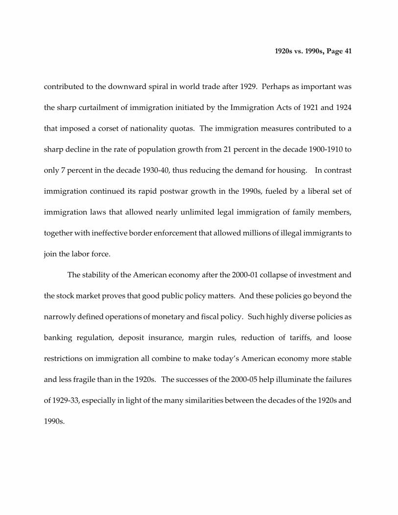
contributed to the downward spiral in world trade after 1929. Perhaps as important was

the sharp curtailment of immigration initiated by the Immigration Acts of 1921 and 1924

that imposed a corset of nationality quotas. The immigration measures contributed to a

sharp decline in the rate of population growth from 21 percent in the decade 1900-1910 to

only 7 percent in the decade 1930-40, thus reducing the demand for housing. In contrast

immigration continued its rapid postwar growth in the 1990s, fueled by a liberal set of

immigration laws that allowed nearly unlimited legal immigration of family members,

together with ineffective border enforcement that allowed millions of illegal immigrants to

join the labor force.

The stability of the American economy after the 2000-01 collapse of investment and

the stock market proves that good public policy matters. And these policies go beyond the

narrowly defined operations of monetary and fiscal policy. Such highly diverse policies as

banking regulation, deposit insurance, margin rules, reduction of tariffs, and loose

restrictions on immigration all combine to make today’s American economy more stable

and less fragile than in the 1920s. The successes of the 2000-05 help illuminate the failures

of 1929-33, especially in light of the many similarities between the decades of the 1920s and

1990s.

1920s vs. 1990s, Page 42

1920s vs. 1990s, Page 43

REFERENCES

Balke, Nathan S., and Gordon, Robert J. (1986). “Appendix B: Historical Data,” in Gordon,ed., (1986), pp. 781-850.

Basu, Susanto, Fernald, John G., Oulton, Nicholas, and Srinivasan, Sylaja. 2003. ““The Caseof the Missing Productivity Growth, or, Does Information Technology Explain WhyProductivity Accelerated in the United States But Not the United Kingdom?” NBERMacroeconomics Annual 2003, pp. 9-63.

David, Paul A. (1990). “The Dynamo and the Computer: An Historical Perspective on theModern Productivity Paradox,” American Economic Review, vol. 80(2), May, pp. 355-61.

__________ (1991) “Computer and Dynamo: The Modern Productivity Paradox in a Not-too-distant Mirror.” In G. Bell, ed., Technology and Productivity. Paris: OECD.

___________ and Wright, Gavin (2000). “General Purpose Technologies and Surges inProductivity: Historical Reflections on the Future of the ICT Revolution,” in P. A.David and M. Thomas, The Economic Future in Historical Perspective. Oxford: OxfordUniversity Press for the British Academy.

Economic Report of the President, 2003. Washington, February.

Eichengreen, Barry (1992a). Golden Fetters: The Gold Standard and the Great Depression, 1919-1939. New York and Oxford: Oxford University Press.

___________ (1992b). “The Origins and Nature of the Great Slump Revisited,” EconomicHistory Review, vol. 45, no. 2 (May), pp. 213-39.

__________ (2000). ʺU. S. Foreign Financial Relations in the Twentieth Century,ʺ inEngerman and Gallman, eds., pp. 463-504.

Engerman, Stanley L., and Gallman, Robert E. (2000). The Cambridge Economic History of theUnited States: Volume III, The Twentieth Century. Cambridge UK: CambridgeUniversity Press.

1920s vs. 1990s, Page 44

Friedman, Milton, and Schwartz, Anna Jacobson (1963). A Monetary History of the UnitedStates: 1867-1960. Princeton: Princeton University Press for NBER.

Goldin, Claudia, and Margo, Robert (1992). “The Great Compression: The U. S. WageStructure at Mid-Century,” Quarterly Journal of Economics, vol. 107, no. 1 (February).

Goldin, Claudia, and Katz, Lawrence (1998). “The Origins of Technology-SkillComplementarity,” Quarterly Journal of Economics, vol 113, pp. 693-732.

Gordon, Robert Aaron (1951). “Cyclical Experience in the Interwar Period: The InvestmentBoom of the `Twenties’,” in Universities-National Bureau Committee, Conference onBusiness Cycles. New York: National Bureau of Economic Research.

__________ (1961). Business Fluctuations, second edition. New York: Harper and Brothers.

___________ (1974). Economic Instability and Growth: The American Record. New York:Harper & Row.

Gordon, Robert J. (1982). “Why Stopping Inflation May Be Costly: Evidence from FourteenHistorical Episodes,” in Hall, Robert E., ed., Inflation: Causes and Effects. Chicago:University of Chicago Press, pp. 11-40.

Gordon, Robert J., ed. (1986) The American Business Cycle: Continuity and Change.University of Chicago Press for NBER.

__________ (1997). “The Time-Varying NAIRU and Its Implications for Economic Policy,”Journal of Economic Perspectives, vol. 11, no. 1, pp. 11-32.

__________ (1998). “Foundations of the Goldilocks Economy: Supply Shocks and the Time-Varying NAIRU,” Brookings Papers on Economic Activity, vol. 29, no. 2, pp. 297-333.

__________ (2000a). ʺInterpreting the `One Big Waveʹ in U. S. Long-term ProductivityGrowth,ʺ in Bart van Ark, Simon Kuipers, and Gerard Kuper, eds., Productivity,Technology, and Economic Growth. Boston: Kluwer Publishers, pp. 19-65.

___________ (2000b). “Does the New Economy Measure Up to the Great Inventions of thePast?” Journal of Economic Perspectives, vol. 14, no. 4 (Fall), pp. 49-74.

1920s vs. 1990s, Page 45

___________ (2003). Macroeconomics, ninth edition. Boston: Addison-Wesley.

___________ and Veitch, John M. (1986). ̋ Fixed Investment in the American Business Cycle,1919-83,ʺ in Gordon (1986), pp. 267-357.

__________ and Wilcox, James (1981). ̋ Monetarist Interpretations of the Great Depression:Evaluation and Critique,ʺ in Karl Brunner, ed., The Great Depression Revisited.Boston: Martinus Nijhoff, pp. 49-107.

Hickman, Bert G. (1974). “What Became of the Building Cycle?” In Paul A. David andMelvin Reder, eds., Nations and Households in Economic Growth: Essays in Honor ofMoses Abramovitz. New York: Academic Press.

Hicks, John R. (1950). A Contribution to the Theory of the Trade Cycle. Oxford: ClarendonPress.

Jorgenson, Dale W, and Stiroh, Kevin J. 2000. ʺRaising the Speed Limit: U. S. EconomicGrowth in the Information Age,ʺ Brookings Papers on Economic Activity, vol. 31, no. 1,pp. 125-211.

Keegan, John (1989). World War II. London: Hutchinson.

Kendrick, John W. (1961). Productivity Trends in the United States. Princeton UniversityPress for NBER.

Kurian, George T. (2001). Datapedia of the United States: 1790-2005. Lanham MD: Bernan.

Lebergott, Stanley (1964). Manpower in Economic Growth: The United States Record Since 1800.New York: McGraw-Hill.

Long-term Economic Growth 1860-1970 (1973). Washington: U. S. Department of Commerce.

Oliner, Stephen D., and Sichel, Daniel E. 2000. ̋ The Resurgence of Growth in the Late 1990s:Is Information Technology the Story?ʺ Journal of Economic Perspectives, vol. 14, Fall,pp. 3-22.

1920s vs. 1990s, Page 46

__________. 2002. ʺInformation Technology and Productivity: Where Are We Now andWhere Are We Going?ʺ Economic Review, Federal Reserve Bank of Atlanta, third quarter:15-44.

Olmstead, Alan L., and Rhode, Paul W. (2000). “The Transformation of NorthernAgriculture, 1910-1990.” in Engerman and Gallman, eds., pp. 693-742.

Piketty, Thomas, and Saez, Emmanuel (2003). “Income Inequality in thee United States,1913-1998,” Quarterly Journal of Economics, vol. 118, no. 1, February, pp. 1-35.

Plotnick, Robert D., et. al. (2000). “The Twentieth-Century Record of Poverty and Inequalityin the United States,” in Engerman and Gallman, eds. (2000), pp. 249-99.

Samuelson, Paul A. (1939). “Interactions between the Multiplier Analysis and the Principleof Acceleration, “ Review of Economic Statistics, vol. 21, No. 2. (May), pp. 75-78.

Schumpeter, Joseph A. (1939). Business Cycles. New York: McGraw-Hill.

Staiger, Douglas, Stock, James H., and Watson, Mark W. (1997). “The NAIRU,Unemployment, and Monetary Policy,” Journal of Economic Perspectives, vol. 11, no.1, pp. 33-49.

Statistical Abstract of the United States (1996, 2002). Washington: U. S. Department ofCommerce.

Temin, Peter (1976). Did Monetary Forces Cause the Great Depression? New York: Norton.

__________ (2000). ʺThe Great Depression,ʺ in Engerman and Gallman, eds., pp. 301-28.

White, Eugene N. (2000). “Banking and Finance in the Twentieth Century,” in Engermanand Gallman (2000), pp. 743-802.

Yang, Shinkyu, and Brynjolfsson, Erik (2001.) “Intangible Assets and Growth Accounting:Evidence from Computer Investments.” Unnumbered working paper, M.I.T., May.

1920s vs. 1990s, Page 47

DATA APPENDIX

All data for the 1990’s were obtained from the Economic Report of the President, 2003, theStatistical Abstrct, 1996 and 2002, Gordon’s Macroeconomics (2003), and the websites of the Bureau ofLabor Statistics (BLS; www.bls.gov) and the Bureau of Economic Analysis (BEA; www.bea.gov). These data were current as of March 12, 2004 and were retrieved for the period 1984 to 2003.

The BLS data are identified by their BLS series identifier.

Consumer Price Index CUUR0000SA0

For the Nonfarm private business sector:

Output PRS85006043

Aggregate Hours PRS85006033

Productivity PRS85006093

All data obtained from the BEA website came from the National Income and Product Accounts(NIPA). National income data came from table 1.7.5, and data on dividends and interest came fromtable 1.14.

The Economic Report of the President was the source for data on employee compensation (table B-14),proprietor’’s income, rent (both table B-28), Employment, Labor force, and population (all from thehousehold survey, table B-35), Treasury bill discount rate (table B-73), and the level of the Standardand Poor’’s 500 index of stocks (table B-95). Nominal and Real GDP, GDP deflator, and moneysupply (M2), were obtained from Gordon (2003). The Statistical Abstract was the source forelectricity output (table T 1065), the fraction of people with access to a computer at home or at work(tables T657 and T 1197), and the fraction of people with internet access at home or at work (tableT1134). Data for electricity output for 1990 and the 1920’s came from Datapedia (series Q152) and for2000 came from SA 2002 (series T 1065)

Data for the 1920’’s was obtained from the National Bureau of Economic Review MacrohistoryDatabase (NBER; www.nber.org), Productivity Trends in the United States (Kendrick, 1961), LTEG,and Datapedia. These data were retrieved for the period 1913 to 1932. Where possible, this data were“ratio linked” to the modern data. Given an overlapping year, generally 1929, the data for the 1910sand 1920s were multiplied by the ratio of the modern series to the historical series.

Data from the NBER database are identified by their series number. All data that were in quarterlyor monthly form were interpolated to annual averages.

National Income a08167

1920s vs. 1990s, Page 48

Employee Compensation a08181

Rent a08184

Dividends a08185

Interest a08186

Data from Kendrick (1961) include output, hours, productivity (table A-XXII), and hours peremployee (table A-IX). LTEG was the source for household employment (series A78), unemploymentrate (series B1), labor force participation rate (series B9), treasury bill discount rate (series B-82), andthe level of the S&P 500 (series B84) The number of motor vehicle registrations and electricity outputwas obtained from Datapedia (series Q152 and S32, respectively).

The expenditure shares for the period 1929-2003 in Figures 6-9 were obtained from the BEA web site,series 1.10. Series for the 1920s were constructed initially by linking consumption, investment,government spending, and net exports from Kendrick (1961, Table AIIa) to the current BEA chain-weighted numbers, which places all the ratios for the 1920s on the basis of 1929 price weights. Thenthe subcomponents of consumption and investment were obtained from Balke-Gordon (1986), whichin turn developed these measures from the sources cited there.

Figure 1. Real GDP

40

50

60

70

80

90

100

110

1913

:1984

1914

:1985

1915

:1986

1916

:1987

1917

:1988

1918

:1989

1919

:1990

1920

:1991

1921

:1992

1922

:1993

1923

:1994

1924

:1995

1925

:1996

1926

:1997

1927

:1998

1928

:1999

1929

:2000

1930

:2001

1931

:2002

1932

:2003

1913-1932

1984-2003

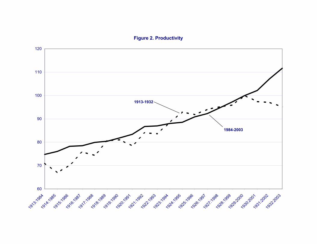
Figure 2. Productivity

60

70

80

90

100

110

120

1913

:1984

1914

:1985

1915

:1986

1916

:1987

1917

:1988

1918

:1989

1919

:1990

1920

:1991

1921

:1992

1922

:1993

1923

:1994

1924

:1995

1925

:1996

1926

:1997

1927

:1998

1928

:1999

1929

:2000

1930

:2001

1931

:2002

1932

:2003

1913-1932

1984-2003

Figure 3. Unemployment

0.0

5.0

10.0

15.0

20.0

25.0

30.0

1913

:1984

1914

:1985

1915

:1986

1916

:1987

1917

:1988

1918

:1989

1919

:1990

1920

:1991

1921

:1992

1922

:1993

1923

:1994

1924

:1995

1925

:1996

1926

:1997

1927

:1998

1928

:1999

1929

:2000

1930

:2001

1931

:2002

1932

:2003

1913-1932

1984-2003

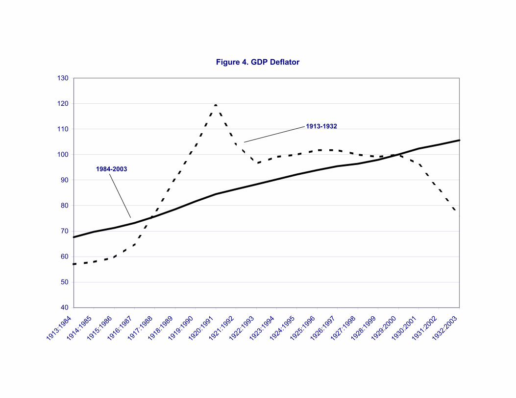
Figure 4. GDP Deflator

40

50

60

70

80

90

100

110

120

130

1913

:1984

1914

:1985

1915

:1986

1916

:1987

1917

:1988

1918

:1989

1919

:1990

1920

:1991

1921

:1992

1922

:1993

1923

:1994

1924

:1995

1925

:1996

1926

:1997

1927

:1998

1928

:1999

1929

:2000

1930

:2001

1931

:2002

1932

:2003

1913-1932

1984-2003

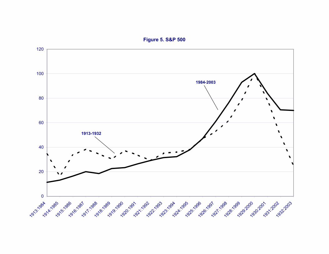
Figure 5. S&P 500

0

20

40

60

80

100

120

1913

:1984

1914

:1985

1915

:1986

1916

:1987

1917

:1988

1918

:1989

1919

:1990

1920

:1991

1921

:1992

1922

:1993

1923

:1994

1924

:1995

1925

:1996

1926

:1997

1927

:1998

1928

:1999

1929

:2000

1930

:2001

1931

:2002

1932

:2003

1913-1932

1984-2003

Figure 6. Share in Real GDP of Consumer Durables and Total Investment, 1919-32 and 1990-2003

0

5

10

15

20

25

30

1919

:1990

1920

:1991

1921

:1992

1922

:1993

1923

:1994

1924

:1995

1925

:1996

1926

:1997

1927

:1998

1928

:1999

1929

:2000

1930

:2001

1931

:2002

1932

:2003

1913-19321984-2003

Figure 7. Shares in Real GDP of PDE and Software, and of Consumer Durables, 1919-32 and 1990-2003

0

1

2

3

4

5

6

7

8

9

10

1919

:1990

1920

:1991

1921

:1992

1922

:1993

1923

:1994

1924

:1995

1925

:1996

1926

:1997

1927

:1998

1928

:1999

1929

:2000

1930

:2001

1931

:2002

1932

:2003

PDE and Software, 1919-1932

PDE and Software, 1990-2003

Consumer Durables, 1919-1932

Consumer Durables, 1990-2003

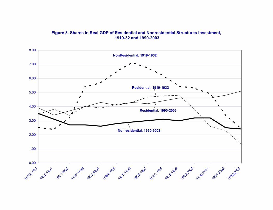
Figure 8. Shares in Real GDP of Residential and Nonresidential Structures Investment, 1919-32 and 1990-2003

0.00

1.00

2.00

3.00

4.00

5.00

6.00

7.00

8.00

1919

:1990

1920

:1991

1921

:1992

1922

:1993

1923

:1994

1924

:1995

1925

:1996

1926

:1997

1927

:1998

1928

:1999

1929

:2000

1930

:2001

1931

:2002

1932

:2003

Nonresidential, 1990-2003

NonResidential, 1919-1932

Residential, 1990-2003

Residential, 1919-1932

Figure 9. Share in Real GDP of Inventory Change, 1919-32 and 1990-2003

-5.00

-4.00

-3.00

-2.00

-1.00

0.00

1.00

2.00

3.00

4.00

5.00

6.00

1919

:1990

1920

:1991

1921

:1992

1922

:1993

1923

:1994

1924

:1995

1925

:1996

1926

:1997

1927

:1998

1928

:1999

1929

:2000

1930

:2001

1931

:2002

1932

:2003

1919-1932

1990-2003

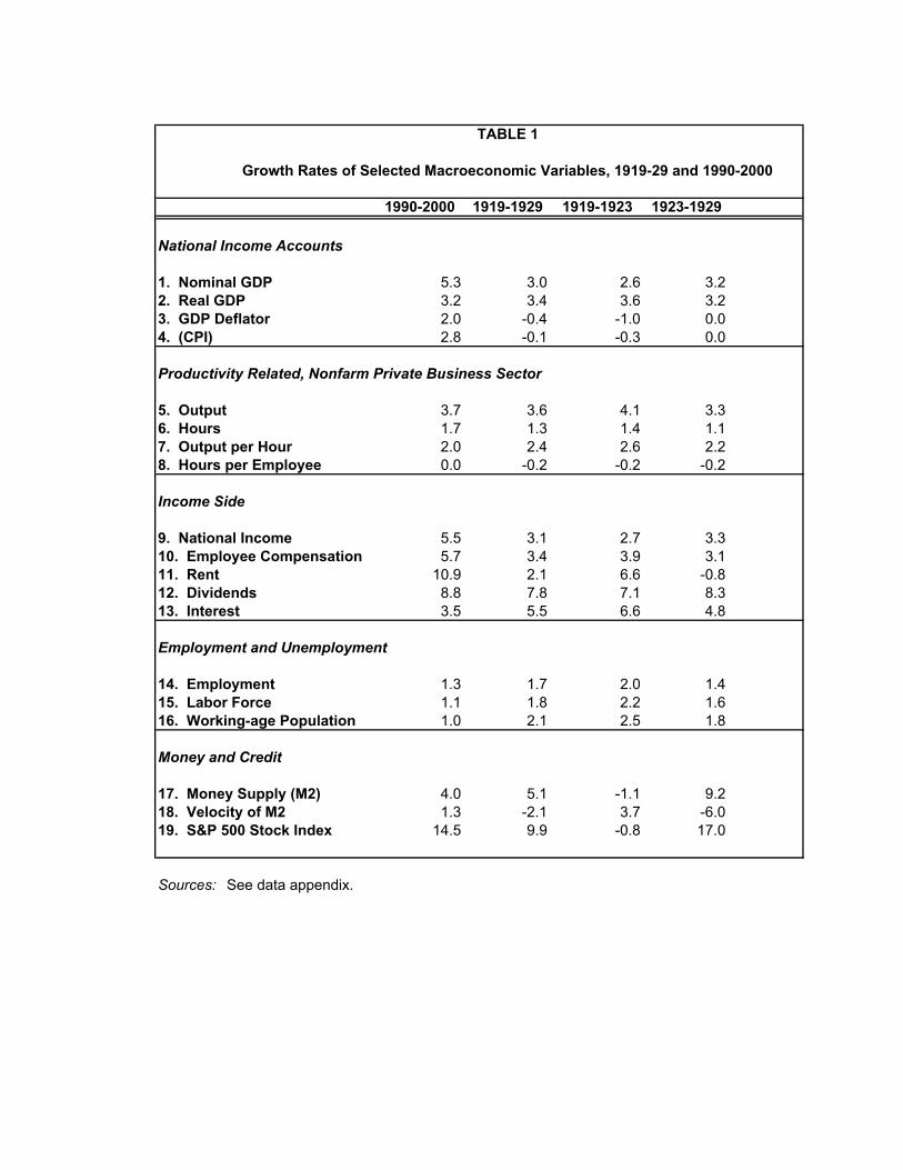
TABLE 1

Growth Rates of Selected Macroeconomic Variables, 1919-29 and 1990-2000

1990-2000 1919-1929 1919-1923 1923-1929

National Income Accounts

1. Nominal GDP 5.3 3.0 2.6 3.22. Real GDP 3.2 3.4 3.6 3.23. GDP Deflator 2.0 -0.4 -1.0 0.04. (CPI) 2.8 -0.1 -0.3 0.0

Productivity Related, Nonfarm Private Business Sector

5. Output 3.7 3.6 4.1 3.36. Hours 1.7 1.3 1.4 1.17. Output per Hour 2.0 2.4 2.6 2.28. Hours per Employee 0.0 -0.2 -0.2 -0.2

Income Side 9. National Income 5.5 3.1 2.7 3.310. Employee Compensation 5.7 3.4 3.9 3.111. Rent 10.9 2.1 6.6 -0.812. Dividends 8.8 7.8 7.1 8.313. Interest 3.5 5.5 6.6 4.8

Employment and Unemployment

14. Employment 1.3 1.7 2.0 1.415. Labor Force 1.1 1.8 2.2 1.616. Working-age Population 1.0 2.1 2.5 1.8

Money and Credit

17. Money Supply (M2) 4.0 5.1 -1.1 9.218. Velocity of M2 1.3 -2.1 3.7 -6.019. S&P 500 Stock Index 14.5 9.9 -0.8 17.0

Sources: See data appendix.

TABLE 2

Levels of Selected Macroeconomic Variables, 1919-29 and 1990-2000

1919 1929 1990 2000

National Income Accounts

1. Nominal GDP ($ bil) 76.9 103.6 5803.1 9817.02. Real GDP ($2000 bil) 614.9 865.2 7112.5 9817.03. GDP Deflator (2000=100) 12.5 12.0 81.6 100.04. CPI (1967 = 100) 51.8 51.3 391.4 511.8

Employment and Labor Force

5. Employment (mil) 39.2 46.2 118.8 135.26. Labor Force (mil) 39.7 47.7 125.8 140.97. Working-Age Population (mil) 70.4 86.6 189.2 209.78. Unemployment Rate (percent) 1.4 3.2 5.6 4.09. Labor-Force Participation Rate (percent) 56.4 55.1 66.5 67.210. Real GDP per Employee ($2000 '000) 15.7 18.7 59.9 72.6

Interest Rates and Stock Market

10. Treasury Bill Rate (percent) 4.9 4.4 7.5 5.911. Real Treasury Bill Rate (percent) 4.9 4.4 4.3 4.211. S&P 500 Stock Price Index (1941-43 = 10) 8.8 26.0 335.3 1427.2

New Industries

12. Automobile Registrations (mil.) 7.6 26.7 188.7 221.513. Electricity Generation (bil KWH) 52.3 116.7 2816.7 3606.514. Computer Use at Home or Work (mil) ---- ---- 73.7 174.0