NBER WORKING PAPER SERIES

NEW EVIDENCE ON THE CAUSAL LINKBETWEEN THE QUANTITY AND QUALITY OF CHILDREN

Joshua D. AngristVictor Lavy

Analia Schlosser

Working Paper 11835http://www.nber.org/papers/w11835

NATIONAL BUREAU OF ECONOMIC RESEARCH1050 Massachusetts Avenue

Cambridge, MA 02138December 2005

Special thanks go to the staff of the Central Bureau of Statistics in Jerusalem, without whose assistance thisproject would not have been possible. We also thank Oded Galor, Omer Moav, Shaul Lach, Yaacov Ritov,Yona Rubinstein, Avi Simchon, David Weil and seminar participants at the 2005 NBER Summer Institute,Brown, and SUNYAlbany for helpful discussions and comments. The results reported here are preliminaryand part of an ongoing study. The views expressed herein are those of the author(s) and do not necessarilyreflect the views of the National Bureau of Economic Research.

©2005 by Joshua D. Angrist, Victor Lavy, and Analia Schlosser. All rights reserved. Short sections of text,not to exceed two paragraphs, may be quoted without explicit permission provided that full credit, including© notice, is given to the source.

New Evidence on the Causal Link Between the Quantity and Quality of ChildrenJoshua D. Angrist, Victor Lavy, and Analia SchlosserNBER Working Paper No. 11835December 2005JEL No. J13, I31

ABSTRACT

A longstanding question in the economics of the family is the relationship between sibship size and

subsequent human capital formation and economic welfare. If there is a “quantity-quality trade-off,”

then policies that discourage large families should lead to increased human capital, higher earnings,

and, at the macro level, promote economic development. Ordinary least squares regression estimates

and a large theoretical literature suggest that this is indeed the case. This paper provides new

evidence on the child-quantity/child-quality trade-off. Our empirical strategy exploits exogenous

variation in family size due to twin births and preferences for a mixed sibling-sex composition, as

well as ethnic differences in the effects of these variables, and preferences for boys in some ethnic

groups. We use these sources of variation to look at the causal effect of family size on completed

educational attainment, fertility, and earnings. For the purposes of this analysis, we constructed a

unique matched data set linking Israeli Census data with information on the demographic structure

of families drawn from a population registry. Our results show no evidence of a quantity-quality

trade-off, though some estimates suggest that first-born girls from large families marry sooner.

Joshua D. AngristDepartment of EconomicsMIT, E52-35350 Memorial DriveCambridge, MA 02142-1347and NBERangrist@mit.edu

Victor LavyDepartment of EconomicsHebrew UniversityJerusalem 91905Israeland NBERmsvictor@huji.ac.il

Analia SchlosserDepartment of EconomicsHebrew UniversityJerusalem 91905Israelani@mscc.huji.ac.il

1

FAMILY PLANNING: THE WAY TO PROSPERITY. (A SLOGAN FOUND ON THE BACK OF INDONESIA’S FIVE-RUPIAH COIN) I. Introduction

The question of how family size affects economic circumstances is one of the most enduring in social science.

The earliest theoretical discussion of the role of family size in the determination of living standards was

probably by Malthus, who famously argued that family size responds to income shocks in a manner that

keeps living standards at a constant subsistence level. Beginning with Becker and Lewis (1973) and Becker

and Tomes (1976), economists have replaced the Malthusian model with a theoretical framework that sees

both the number of children and parental investment per child as choice variables that respond to economic

forces. Part of this agenda is an attempt to reconcile the apparent paradox of declining family size in the face

of economic growth with the superficially plausible presumption that children are indeed a normal good. The

notion of a quantity-quality trade-off appears to provide this reconciliation: as parents get richer they demand

children of higher “quality,” (i.e., children who are more productive), without necessarily demanding more of

them. In fact, because increases in quality can be interpreted as making children more expensive, the

quantity-quality trade-off explains why families might get smaller as parents get richer.

On the policy side, the notion that smaller families and slower population growth are essential for

development motivates many governments and international agencies to promote, or even to require smaller

families.1 While this policy position often seems to be based on naive empiricism, both the Malthusian and

the Becker and Lewis (1973) models provide some theoretical support for the view that large families keep

living standards low. A negative causal relation between child quantity and parental investment also comes

out of a number of sophisticated theoretical recent analyses of the role of the demographic transition in

economic development (e.g., Galor and Weil, 2000; Hazan and Berdugo, 2002, and Moav, 2005). On the

1In addition to China, examples of government-sponsored family planning efforts include a forced-sterilization

program in India and the aggressive public promotion of family planning in Mexico and Indonesia. These episodes are recounted in Weil (2005; Chapter 4), which also mentions the antinatalist slogan on the Indonesian Rupiah. Bongaarts (1994) notes that by 1990, 85 percent of people in the developing world lived in countries where the government considered the rates of fertility too high.

2

other hand, the newer theories focus primarily on the quantity and quality implications of human capital

accumulation. In these models, the effects of population-control efforts and similar policy interventions are

less clear cut, a point we return to after discussing the estimates.

Most of the scholarly evidence pointing to an empirical quantity-quality trade-off comes from the

widely observed negative association between family size on one hand and schooling or achievement on the

other. For example, Leibowitz (1974) and Hanushek (1992) find that children’s educational attainment and

achievement growth are negatively correlated with family size. Many other micro-econometric and

demographic studies show similar relations.2 The principal problem with research of this type is that such

associations are not necessarily indicative of a causal relation. The fact that people raised in large families

end up with less schooling than those raised in smaller families need not be due to family size per se. Rather,

this correlation may simply reflect differences in parental education, earnings potential, or other potentially

unobserved factors that affect both fertility and the home environment. The likelihood of omitted variables

bias in estimates of the effects of childbearing is highlighted by Angrist and Evans (1998), who used multiple

births and preferences for a mixed sibling-sex composition to construct instrumental variables (IV) estimates

of the effect of family size on mothers’ labor supply. IV estimates using both twins and same-sex

instruments, while still negative, are considerably smaller than the corresponding OLS estimates.

This paper provides new evidence on the quantity-quality trade-off using exogenous variation in

family size. Our approach adapts and extends the Angrist-Evans (AE-98) IV strategy to the estimation of

effects of family size on various measures of “quality” that might be affected by the home environment. In

particular, we look at the effect of third and higher births on first- and second-born children’s completed

schooling, adult earnings, and on marital status and fertility. Two of the instruments used here, as in AE-98,

are dummies for multiple births at second birth and a dummy for same-sex sibling pairs in families with two

2See, e.g., the recent review by Schultz (2005). Johnson (1999) notes that the relation between family size and

economic well being or growth is less clear cut at the time series or cross-country level. In contrast with Hanushek (1992), Guo and Vanwey (1999) show that control for family effects eliminates the relation between sibship size and intellectual development.

3

or more children.

We also extend the AE-98 identification strategy in a number of ways. First, in addition to looking at

families with two or more children, we exploit multiple third births and the effects of sibling-sex composition

in families with three or more children. We also introduce a new source of exogenous variation in family size

based on sharp differences in the effects of multiple births and sex-composition across ethnic groups in the

Israeli population. For example, multiple births have a much larger effect on Jews of European or North

American origin than on Jews of Asian or North African origin, since the latter chose to have large families

even in the absence of a multiple birth. On the other hand, an all-female sibling sex composition leads to

sharp rise in the number of children born to the Asia-Africa group, with relatively little effect on the fertility

of ethnic Europeans and Israeli natives. Finally, we exploit preferences for boys at higher order births in the

Asia-Africa subsample. Thus, our sample and identification strategies allow us to juxtapose the results from a

number of different groups, using fertility shocks of different sorts and sizes, and over differing ranges of

variation. Remarkably, all of this evidence points in the same direction: an exogenous increase in family size

at second and higher births appears to have little effect on first and second born children, with the possible

exception of an increase in the likelihood that female children marry.

Our paper comes on the heels of a substantial and growing literature attempting to link multiple births

with measures of child quality. Rosenzweig and Wolpin (1980) appear to have been the first to use multiple

births to estimate a child-quantity/child-quality trade-off. More recent estimates using multiple births include

Duflo (1998), who looks at effects on child mortality in Indonesia; Black, Devereux, and Salvanes (2004),

who estimate effects on education in Norway; and Caceres (2004), who looks at effects on private school

enrollment in US Census data. Caceres (2004) also estimates effects on dropout status, teen pregnancy, and

parents’ marital status.

An important difference between our study and these earlier papers is that we have a wider range of

outcomes than has been previously available for a research design of this type. Our outcomes come from a

unique data set we constructed for the purposes of this project linking the 1983 and 1995 Israeli Census micro

4

samples, which provide information on education, work, earnings, marriage, and childbearing, with detailed

sibling information from the population registry. A second key difference is that the ethnic diversity of the

Israeli population allows us to compare effects across families of different sizes and from different cultural

traditions. Of particular interest here are results for the Asia-Africa subsample, that is, Sephardic Jews of

North African and Middle Eastern origin. Those in this group have demographic and social characteristics

much closer to developing country populations than do native-born Israelis or Israelis of European and North

American stock. Finally, ours appears to be the first study to use sibling-sex composition to estimate the

quality-quantity trade-off for a wide range of outcomes, or with a strong and well-documented first-stage.3

The paper is organized as follows. The next section describes the census-registry link and the

construction of our more-than-two (2+) and more-than-three (3+) analysis samples. Section III discusses

first-stage estimates and Section IV presents the main OLS and 2SLS results. We discuss the relation

between our findings and earlier work in Section V, focusing on the question of whether the case for an

empirical quantity-quality trade-off should be evaluated in terms of parental inputs or child outcomes.

Finally, Section VI concludes and suggests directions for further work.

II. Data and Samples

The main sources of data used here are the 20% public-use micro-data samples from the 1995 and

1983 Israeli censuses, linked with information on parents from the population registry. The Israeli census

micro files are 1-in-5 random samples that include information collected on a fairly detailed long-form

questionnaire similar to the one used to create the PUMS files for US censuses.4 The set of Jewish long-form

3Black, Devereux, and Salvanes (2004) briefly mention a failed effort in this direction. Conley and Glauber

(2004) report estimates using sex-composition IVs, looking at grade retention and private school attendance, though problems with their research design make their results hard to interpret. Lee (2004) uses preferences for male children to construct an instrument for family size in Korea, where preferences for boys (as opposed to a mixed sibling-sex composition) are strong.

4Documentation can be found at the Israel Social Sciences Data Center web site: http://isdc.huji.ac.il/mainpage_e.html (data sets 115 [1995 demographic file] and 301 [1983 files]). The Census includes residents of dwellings inside the State of Israel and Jewish settlements in the occupied territories. This includes residents

5

respondents aged 18-60 provides our initial study sample. In the discussion that follows, we refer to these

individuals as “subjects,” to distinguish them from their parents and siblings, for whom we also collected

data. Information on parents and siblings was obtained from the Israeli population registry maintained by the

ministry of the interior. Conditional on an ongoing confidentiality review, the registry is available for use on

a per-project basis inside the Central Bureau of Statistics (CBS) in a restricted-access Research Data Center.

The link from census to registry is necessary for our purposes because in a sample of adult respondents, most

of who no longer live with their parents and siblings, the census provides no information about sibship size,

multiple births, or sibling sex composition.5

The Israeli population registry, our source of information on families of origin, contains updated

administrative records for Israeli citizens and residents, whether currently living or dead, including most

Israelis who have moved abroad. This data base also includes the Israeli ID numbers held by citizens and

temporary residents. ID numbers are issued at birth for the native-born and upon arrival for immigrants. In

addition to basic demographic information on individuals (date of birth, sex, country of birth, year of

immigration, marital status, religion and nationality), the registry records parents’ names and registrants’

parents’ ID numbers.

The construction of our analysis file proceeded by first using our subject’s ID numbers to link to non-

public-use versions of census long-form files that include ID numbers with registry records for as many

subjects as we could find. In a second step, we used the registry to find subjects’ mothers. Finally, once

mothers were linked to census respondents, we then located all the mothers’ children in the registry, whether

or not these children appear in the census. In this manner we were able to observe the sex and birth dates of

most adult census respondents’ siblings.

abroad for less than one year, new immigrants, and non-citizen tourists and temporary residents living at the indicated address for more than a year.

5About 80% of the Israeli population is Jewish. The study sample is limited to Jews because census-to-population-registry match rates are considerably lower for other groups.

6

Match Rates and Sample Selection

Although coverage rates are reasonably good, not all census respondents appear in the population

registry. Moreover, among those who can be found, information may be missing for mothers, and among

those with mothers in the registry, some or all siblings may be missing. The likelihood of successful matches

at each stage of our linkage effort is determined primarily by the inherent coverage limitations of the registry.

Israel’s population registry was first developed in 1948, not long after the creation of the state of Israel.

Census enumerators went from house to house, simultaneously collecting information for the first census and

for the administrative system that became the registry. Later, the registry was updated using vital statistics

data. Thus, in principle, the sample of respondents available for a census interview in 1983 and 1995 should

appear in the registry, along with their mothers’ ID numbers, if they were resident in Israel in 1948, born in

Israel after 1948, or immigrated to Israel after 1948.

The vast majority of our subjects do indeed appear in the registry. This can be seen in Table 1, the

first two rows of which report starting sample sizes and subject-to-registry match rates, grouped according to

whether subjects’ parents were Israeli born, birth cohort, and whether subjects were Israeli-born (there are

two panels in the table, one for each census). Subject-to-registry match rates range from 95-97 percent

regardless of cohort and nativity. The most relevant coverage shortfall from our point of view is the failure to

obtain an administrative record for subjects’ mothers. This failure arises for a number of reasons. First,

subject’s mothers may have been alive but not at home in 1948 when the registry was created, or the mother

may have been deceased. Second, and more importantly for most of our subjects, children are linked to

mothers at the time they are born. We are therefore most likely to locate all of a subject’s siblings when the

subject’s mother gave birth to all of her children in Israel.

The second row of each panel in Table 1 describes the impact of these record-keeping constraints on

our census-to-registry match rates. The mothers of subjects with Israeli-born fathers were found 90 percent

of the time for cohorts born after 1955. On the other hand, for those born before 1955, only 17 percent of

mothers were found. Likewise, for those with foreign-born fathers, there is a similar age gradient in mothers’

7

match rates. Even in this group, however, 87 percent of mothers were found for younger Israeli-born subjects

in the 1995 census. The 1955 birth cohort marks a natural division for our purposes because mothers of

subjects born after 1954 gave birth to most of their children in post-1948 Israel (the mothers in this group

were mostly born after 1930, and, assuming childbirth starts at 18, this dates their first births at 1948 or later).

Given the match rates in Table 1, our analysis sample is clearly weighted towards post-1955 cohorts

(i.e., 40 or younger in 1995). This accounts for about two-thirds of the 1995 population aged 18-60. Among

the children of immigrant fathers, we’re also much more likely to find mothers of the Israeli-born. The

coverage rates for post-1955 Israeli-born cohorts seem high enough that we are likely to have information on

mothers for a representative sample of younger cohorts regardless of fathers’ nativity. For the purposes of

analysis, we also used information on mothers in the matched sample to discard any remaining mothers who

were born before 1930 (as the match rates for this group appeared to be very low anyway). Subjects with

mothers whose first birth was before age 15 or after age 45 were also dropped. These further restrictions

eliminate almost all subjects born before 1955, primarily because most of those born earlier have mothers

born before the 1930 maternal age cutoff. We also restricted the sample of subjects with foreign-born

mothers to those whose mothers arrived 1948 or later and before the age of 45 (in this case so that an

immigrant mother with children is likely to have come with all her children, who would then have been

included in the registry, either in the first census, or at the time IDs were issued to the family).

The final sample restriction retains only first and second-born subjects since these are the people

exposed to the natural experiments exploited by the twins and sex-composition research design. Note that the

restriction to first and second born subjects naturally eliminates a higher percentage of younger rather than

older cohorts. This restriction also has a bigger effect on the Israeli-born children of foreign-born fathers than

on other nativity groups, probably because these children were disproportionately likely to have been born to

immigrant fathers who arrived with a large wave of immigrants from Asia and Africa in the 1950s.

Immigrants from this group typically formed large families after arrival and will therefore have contributed

more higher-parity births to the sample.

8

Description of Analysis Samples

We work with two analysis samples, both described in Table 2. The first sample consists of first-

born subjects in families with two or more births (the 2+ sample, N=89,445). The second sample consists of

first- and second-born subjects in families with three or more births (the 3+ sample, N=65,671 first-born and

53,070 second-born). These samples are defined conditional on the number of births instead of the number of

children so that multiple-birth families can be included in the analysis samples without affecting the sample

selection criteria. Twin subjects were dropped from both samples, however.6

Roughly three-quarters of the observations in each sample were drawn from the 1995 Census. On

average, subjects were born in the mid-sixties and their mothers were in their early twenties at first birth.

because out-of-wedlock childbearing is rare in Israel, especially among the cohorts studied here, virtually all

subjects in both samples were born to married mothers. Naturally, however, some marriages have since

broken up and some wives have been widowed. This is reflected in the 2003 marital status variables available

in the registry.7

The Jewish Israeli population is often grouped by ethnicity, with Jews of African and Asian origin

(AA; e.g., Moroccans), distinguished from Jews of European and North American (EA) origin. The 2+

sample is about 40 percent AA (defined using father’s place of birth), while the 3+ sample is over half AA.

A preference for larger families in the AA population is also reflected in the statistics on numbers of children.

Average family size ranges from 3.6 in the 2+ sample to 4.2 in the 3+ sample (4.3 for second-borns). In the

AA subsample, however, the corresponding family sizes are about 4.3 and 4.7.

Table 2 also reports statistics on the variables used to construct instrumental variables. The twin rate

6A 3+ sample defined as including first-born children from families with three or more children instead of three

or more births would include all families with multiple second births. Likewise, sibling-sex composition can be defined across births without the need to determine which, say, of two twins, constitutes the second child.

7The 2+ sample naturally includes the 3+ sample. In the 3+ sample, about 10 percent of the first- and second-borns have the same mother (both must appear in the 20% census sample and be in the relevant age range). We therefore cluster analyses that pool parities by mothers’ ID.

9

was 9/10 of one percent at second birth in the 2+ sample and 1 percent at third birth in the 3+ sample, with

similar rates in the AA and full samples.8 As expected, about 51 percent of births are male, regardless of

birth order. Consequently, about half of the 2+ sample was born into a same-sex sibling pair and about one-

quarter of the 3+ sample was part of a same-sex threesome.

The outcome variables described in Table 2 measure subjects’ educational attainment, labor market

status and earnings, marital status and fertility, and the characteristics of subjects’ spouses. Most Israelis are

high school graduates, while 20 percent are college graduates. In the AA subsample, however, proportion of

college graduates is much lower. Most of our subjects were working at the time they were interviewed and

earned about 3000 shekels (about 1000 dollars) per month on average (including zeros). About 40 percent of

subjects were married, though marriage rates are higher in the AA subsample. Table 2 also reports select

descriptive statistics on spouses’ characteristics in the sample of married subjects.

III. First-stage Estimates

The twins and same-sex first stages are described below in turn. Because the sex-composition model

is somewhat more complicated in the 3+ sample, these estimates are discussed in a separate subsection.

Twins First-Stages

A multiple second birth increases the number of siblings in the 2+ sample by about half a child, a

statistic reported in column 1 of Table 3, which shows first-stage estimates for the twins experiment. In

particular, column 1 reports estimates of the coefficient α in the equation

ci = Xi′β + αt2i + ηi (1)

where ci is subject i’s sibship size (including the subject), Xi is a vector of controls that includes a full set of

8Note that the second-birth twin rate in the 3+ sample is not comparable to the second birth twin rate in the 2+

sample or the third-birth twin rate in the 3+ sample because the 3+ sample consists of those who had three or more births. Families with a second-born twin need not have a third birth to have three or more children. Families with a second-born twin that have a third birth have at least four children, and hence are relatively rare in the 3+ sample.

10

dummies for subjects’ and subject’s mothers’ ages, Mothers’ age at first birth, mothers’ age at immigration

(where relevant), fathers’ and mothers’ place of birth, census year, and a dummy for missing month of birth.

The variable t2i indicates multiple second births in the 2+ sample.

The Israeli twins-2 first stage is smaller than the twins-2 first stage of about .6 in the AE-98 sample,

reflecting the fact that Israelis typically have larger families than Americans. Multiple births result in a

smaller increase in family size when families would have been large even in the absence of a multiple birth.

Within Israel, however, there are marked differences in the twins first-stage by ethnicity. This can be seen in

column 2 of Table 2, which reports the twins-2 main effect and an interaction term between twins-2 and a

dummy for Asia-Africa ethnicity (ai) in the equation

ci = Xi′β + α0t2i + α1ait2i + ηi. (2)

The twins-2 main effect, α0, captures the effect of a multiple birth in the non-AA population, while the

interaction term, α1, measures the AA/non-AA difference.9 The estimates in column 2 show that non-AA

family size goes up by about .63 in response to a multiple birth (similar to the AE-98 first stage), while AA

family size increases by only .63-.45=.18. Both α0 and α1 are very precisely estimated.

The remaining columns of Table 3 report the first-stage effect of a multiple third birth in the 3+

sample. Twins-3 effects were estimated in the 3+ sample by replacing t2i with t3i, a dummy for multiple third

births, in equations (1) and (2). These results are reported in columns 3-4 for first-borns and columns 5-6 for

the pooled sample of first- and second-borns. The first stage effect of a multiple birth is bigger in the 3+

sample than in the 2+ sample because the desire to have additional children diminishes as family size

increases. For the same reason, the effect of t3i differs less by ethnicity in the 3+ sample than in the 2+

sample, though, as the estimates in column 6 show, there is still a significant difference by ethnicity when

first and second born subjects are pooled.

9 The ai main effect is included in the vector of covariates, Xi.

11

Sibling-Sex Composition First-stage in the 2+ Sample

The sex-composition first stages in the 2+ sample are based on the following two models:

ci = Xi′β + γ1b1i + γ2b2i + πss12i + ηi (3a)

ci = Xi′β + γ1b1i + πbb12i + πgg12i + ηi (3b)

where b1i (boy-first) and b2i (boy-second) are dummies for boys born at first and second birth, the variable

s12i = b1ib2i + (1-b1i)(1-b2i),

is a dummy for same-sex sibling pairs, and

b12i = b1ib2i and g12i = (1-b1i)(1-b2i)

indicate two boys and two girls. Note also that b1i indicates the subject’s sex in the 2+ sample, and that s12i =

b12i+g12i. The first model controls for boy-first and boy-second main effects, while the excluded instrument is

a same-sex effect common to boy and girl pairs. The second model allows the effect of two boys and two

girls to differ, though one of the boy main effects must be dropped since {b1i, b2i, b12i, g12i} are linearly

dependent.10

The same-sex first-stage effects estimated using equation (3a) in the 2+ sample, reported in column 1

of Table 4a, are on the order of .08 children. This increase is due to an increase of a little over .03 in the

likelihood of having more than two children, as well as smaller increases in the likelihood of having more

than 3 and more than 4 children, as can be seen in columns 4, 7, and 8, which report effects on dummies,

dki=1[ci>k], for k=2, 3, and 4. Same-sex sibship at first and second birth has an impact on the likelihood of

having 4 or more children because, with probability one-half at each birth, families with a same-sex sibship

outcome in earlier births find themselves with an all-boy or all-girl sibship at the next birth as well. Thus,

s12i=1 shifts the distribution of fertility to the right in addition to increasing the likelihood that families have

10For example, g12i = 1-b1i-b2i + b12i. Control for boy-first and boy-second main effects is motivated by the fact

that the same-sex interaction term is, in principle, correlated with the main effects (Angrist and Evans, 1998) when the probability of male birth exceeds .5. In practice, however, this matters little because both the correlation is small and because the main effects are small.

12

more than two children.11

Sex-composition effects estimated using equation (3b), allowing for separate two-boys and two-girls

coefficients, are reported in columns 2 and 3 of Table 4a. In addition to allowing different effects for boys

and girls, the results reported in column 3 are from models that incorporate AA interaction terms, as with the

twins estimates discussed above. The effect of two girls is .11 (s.e.=.015) while the effect of two boys is only

.039 (s.e.=.015). The results allowing different effects by ethnicity generate an effect of two girls equal to

.086 (s.e.=.017) in the non-AA population, with the AA effect of two girls is larger by .055 (s.e.=.032). In

contrast, the two boys effect is only .056 (s.e.=.017) in the non-AA population, with the AA two-boys effect

is smaller by .042 (s.e.=.031). As a result, the AA population appears to increase childbearing in response to

the birth of two girls but not in response to the birth of two boys.

The remaining columns of Table 4a show the effect of sibling sex composition on the fertility

distribution for fertility increments above two children. These results are summarized in Figure 1, which

reports first-stage estimates of effects of b12i and g12i on dki for k up to 9, along with the associated confidence

bands. In the AA population, b12i increases the likelihood that families have 3 or more children, with no

significant effect at higher-order births. In contrast, the effect of two girls on dki actually increases from k=2

to k=3, and then tails off gradually, with a marginally significant effect on the likelihood of having 7 or more

children.12 Effects in the non-AA population drop off more sharply as the number of children increases, and

11The first-stage effect of an instrument on ci in the 2+ sample can be shown to be the sum of the first stage

effects on dki; k=2, . . . (Angrist and Imbens, 1995). In contrast with the results reported here, Angrist and Evans (1998) found similar same-sex effects on completed fertility and on the probability of having more than two children, i.e. on d2i,, and therefore chose the latter as the endogenous variable of interest. This difference may be due to the fact that even in the face of a same-sex threesome, relatively few American couples are motivated to try again or because Angrist and Evans did not observe completed fertility. Because of the substantially larger first-stage for ci in the Israeli context, we use completed fertility as the endogenous variable.

12This increase, while counterintuitive at first blush, can be attributed to the fact that in the AA population that ends up with an all-girl triple, the likelihood of having more children is very large. Note that P[ci>k| ci≥k-1]= P[ci>k| ci≥k]P[ci≥k| ci≥k-1]. The first stage effect can be written using the operator ∆s, where this denotes the same-sex contrast in the relevant conditional probability of increasing fertility. We have ∆sP[ci>k| ci≥k-1] = ∆s{P[ci>k| ci≥k]P[ci≥k| ci≥k-1]}=∆sP[ci>k| ci≥k]P[ci≥k| ci≥k-1, si=1]+∆sP[ci≥k| ci≥k-1]P[ci>k| ci≥k, si=0]. For AA, the incremental effects ∆sP[ci>k| ci≥k] and ∆sP[ci≥k| ci≥k-1] are both substantial at k=3,4.

13

are similar for two boys and two girls. If anything, the non-AA population seems to increase childbearing

more sharply in response to two boys than to two girls.

Sibling-Sex Composition First Stages in the 3+ Sample

The sex-composition first-stage in the 3+ sample captures the effect of an all-boy or all-girl triple,

controlling for the sex-composition of earlier births. Because a same-sex triple occurs only in families with

same-sex pairs at first and second births, the model conditions on b12i and g12i, as well as a subject-sex main

effect. An additional variable included in these models is a dummy for the sex of the third child, an effect

which is defined conditional on a mixed-sex sibling pair at first and second birth (because for families with

b12i=1, the boy-third effect is the same as having an all-male triple, while for families with g12i=1, the boy-

third effect is the same as having an all-female triple). The resulting model can be written as follows (we

spell out only the model that allows for separate all-male and all-female effects):

ci = Xi′β + γ1bi + δbb12i + δgg12i + γ3(1-s12i)b3i + λbb123i + λgg123i + ηi, (4)

where b123i and g123i are indicators for all-male and all-female triples and bi is subject sex (i.e., b1i for first-

borns and b2i for second-borns).13

The first-stage effects using equation (4) in the 3+ sample and the corresponding effects after

incorporating the AA interactions are reported in Table 4b. Estimates for the first-borns sample are reported

in columns 1-6. The overall effect of three girls is 0.181 (s.e.=.025), double the effect of three boys, 0.092

(s.e.=.023). As in the 2+ sample, the effect of three girls is bigger in the AA population. The estimate for

non-AA is .097 (s.e.=.032) and the increment for AA is .167 (s.e.=.051). In contrast, the effect of three boys

is similar in the AA and non-AA population. Columns 7-8 in Table 4b report estimates of equation (4) for

total fertility in the pooled sample of first- and second-borns. The estimates are similar to those obtained in

13This model is almost saturated in the sense that it controls for all lower-order interaction terms in the

estimation of the effects of the two samesex triples except for one: in the (1-s12i)b3i term, we don’t distinguish mixed sibling pairs according to whether a boy or girl was born first. There are at most 7 linearly independent terms in any saturated model that conditions on the sex-composition of the first three children, but we have 6. A saturated model is

14

the sample of first-borns only, though they are more precise due to the increased sample size.

Other columns in the table show the effect of sibling sex composition on the probability of having

more than 3 and more than 4 children in the sample of first-borns and in the pooled sample of first- and

second-borns. Since results in both samples are similar, we discuss effects on fertility increments for first-

borns only. These results are summarized in Figure 2, which reports first-stage estimates of the effects of

three-boys/girls (b123i / g123i ) on dki for k=3 to 10, along with the associated confidence bands. The estimates

are from a model that conditions on b12i, g12i and bi, and are estimated separately for the AA and non-AA

population. In the AA population, b123i increases the likelihood of having 4 or more children, with a small and

marginally significant effect on the likelihood of having 5 or more children. The effect of three boys is

similar in the AA and non-AA population. In contrast, the effect of three girls differs considerably by

ethnicity. In the AA population, the effect of g123i increases from k=3 to k=4 and then diminishes gradually

for higher values of k, remaining marginally significant even at k=10. In the non-AA population, in contrast,

the effect of g123i is considerably smaller and differs little from the effect of b123i.

The Boy-3rd Instrument

The fourth and fifth rows of Table 4b show the effect of having a boy at third birth (b3i) in families

with a mixed-sex sibship at first and second birth. A boy at third birth reduces childbearing in families that

already have one boy by .080 (s.e.=.018). Results allowing different coefficients by ethnicity generate an

effect of -.053 (s.e.=.023) in the non-AA population, while the AA interaction term adds a further .054

(s.e.=.035) to this reduction, though the difference between AA and non-AA is not significant. The Boy-3rd

effect potentially provides an additional source of exogenous variation in fertility, beyond pure sex-

composition effects. We therefore add this to the instrument list for some of the 2SLS specifications

discussed below. Figure 3 summarizes the effects of b3i on fertility increments for families with a mixed-sex

obtained by replacing the single term (1-s12i)b3i with two terms, with b1i(1-b2i)b3i and b2i(1-b1i)b3i . In practice, this matters little.

15

sibship at first and second birth, separately by ethnicity. In the AA population, b3i reduces the likelihood of

having more than 4 children as well as the likelihood of higher order births, up to k=7, beyond which the

effect is no longer significant. In the non-AA population, b3i reduces the likelihood of having 4 or more

children, with no significant effect at higher order births.

Pooled First-Stages Using the Full Set of Instruments

In an attempt to increase precision, we also estimated specifications that combine twins and sex-

composition instruments. In particular, for the 2+ sample, we combined the t2i, g12i and b12i. For the 3+

sample, we combined the t3i, g123i, b123i and (1−s12i)b3i instruments, controlling for the characteristics of the

first two births (g12i, b12i, t2i and bi). These models also include AA interactions. Because the results are

similar to those reported in Tables 3, 4a, and 4b, the pooled first stage is reported in the Appendix.

IV. OLS and 2SLS Estimates

The causal effect of interest is the coefficient ρ in the model

yi = Wi′µ + ρci + εi (5)

where yi is an outcome variable and Wi includes the covariates Xi, as well as instrument-specific controls

(e.g., bi). In models without covariates, 2SLS estimates of this equation capture siblings’ weighted average

causal response (ACR) to the birth of an additional child – i.e., the effect of going from ci−1 to ci, averaged

over ci – for those whose parents were induced to have an additional child by the instrument at hand. The

ACR extends the local average treatment effect idea (LATE, Imbens and Angrist, 1994), a causal effect for

those induced to increase childbearing by the instrument, to models with variable treatment intensity. The

weighting function that lies behind the ACR is proportional to the CDF differences plotted in Figures 1-3

(Angrist and Imbens, 1995). With covariates, the interpretation of the ACR is slightly more elaborate, but the

basic idea behind this interpretation is preserved. Of course, OLS estimates of equation (5) need not have a

causal interpretation in models with or without controls.

16

The outcome variables of interest capture the effects of family size on economic well-being and

social status. In particular, we look at measures of subjects’ educational attainment (highest grade completed,

and indicators of high school completion, matriculation status, and college attendance), labor market status

(indicators of work last year and last week, labor force participation, and hours worked last week) and

earnings, marital status (indicators of being married at census day and married by age 21) and fertility

(number of own children and indicators of having any or two or more children), and the characteristics of

subjects’ spouses (years of schooling, last week labor force participation and monthly earnings).

The 2+ Sample

As is typical for regressions of this sort, OLS estimates of the coefficient of family size in equation

(5) imply adverse effects of increased family size on measures of human capital and economic circumstances.

Larger families of origin are also associated with earlier marriage, increased fertility, and marriage to a less

educated spouse. These results can be seen in column 2 of Table 5, which presents OLS estimates for first-

borns in the 2+ sample (column 1 reports the means). Not surprisingly, given the sample sizes, all the OLS

estimates are very precise. Control for covariates reduces but does not eliminate this negative relationship, as

can be seen in column 3 of the table.

In contrast with the adverse effects reflected in the OLS estimates of effects on schooling variables,

2SLS estimates show zero or even positive effects. These results appear in columns 4-8 of Table 5, which

report 2SLS estimates for different sets of instruments. For example, the estimated effect on schooling using

twins instruments with AA interaction terms, reported in column 4, is .101 (s.e.= .13). The corresponding

estimates using sex-composition instruments with AA interaction terms, reported in column 7 is .222

(s.e.=.176). Combining both twins and sex-composition instruments generates an estimate of .15 (s.e.=.104),

reported in column 8. Interestingly, the combination of instruments generates a substantial gain in precision

relative to the use of each instrument set separately. So much so that the estimated schooling effect in the

first row of column 8 is significantly different from the corresponding OLS estimate of −.145 reported in

17

column 3. Likewise, the estimated effect on matriculation status, a key educational milestone in the Israeli

milieu, is small, positive, and reasonably precise.14

This discussion highlights the fact that a key concern with the IV analysis is whether the estimates are

precise enough to be informative. Of particular interest is the ability to distinguish IV estimates from the

corresponding OLS benchmark. As it turns out, the estimates in column 8, constructed by pooling twins and

sex-composition instruments with AA interaction terms, meet this standard of precision remarkably often. In

particular, 12 of the 18 parameters presented in this column are estimated precisely enough that the associated

95% confidence interval exclude the corresponding OLS estimates reported in column 3. Moreover, estimates

of effects on the level and quality of schooling are very close to zero. The least precise estimates are those

for the subject’s own labor market outcomes and his or her spouse’s outcomes. This echoes similar results

reported by Black, Devereux, and Salvanes (2005), who also found insignificant but imprecise effects of

family size on earnings.

A second set of noteworthy findings are those for marriage and fertility. The IV estimates of effects

on marital status suggest that subjects from larger families are more likely to be married and got married

sooner. Using both twins and sex-composition instruments, the estimated effects on marital status are

significantly different from zero and substantially larger than the corresponding OLS estimates. On the other

hand, the marriage effects generated by sex-composition instruments are much larger than the twins

estimates, a point we return to below.

The marriage effects are paralleled by (and are perhaps the cause of) an increase in fertility: the

combination-IV estimate of the effect on the probability of having any children is 0.078, four times larger

then the corresponding OLS estimate, 0.019. Estimates of effects on a dummy for having two or more

children show a similar pattern. In addition to the likelihood that increased marriage rates increase fertility,

these fertility effects may reflect an intergenerational causal link in preferences over family size, a possibility

14 Angrist and Lavy (2004) report that even in a sample limited to those with exactly 12 years of schooling,

matriculation certificate holders earn 13 percent more.

18

suggested by Fernandez and Fogli (2005). Again, however, a cautionary note is that the fertility effects

come from the sex-composition instruments and not twins. Also, since fertility estimates are based on fertility

measures defined as of census day, i.e. 1983 or 1995, they could reflect an effect on earlier childbearing

(possibly generated by earlier marriage) and not on completed fertility. Further record linkage should allow

us to update subjects' fertility through 2004 and address this issue.

The last set of results in Table 5 is for spousal characteristics. Because the sample in this case is

limited to married individuals, these results are potentially affected by selection bias. At the same time, while

they should be interpreted with caution, the spousal results are of interest as an alternative measure of child

quality, beyond human capital and labor market variables. One possible consequence of larger sibship sized

is reduced parental investment in attributes that are rewarded in the marriage market. Consistent with this

notion, and with the other OLS estimates in the table, the OLS estimates in the lower panel of Table 5 suggest

that first-borns from larger families are married to spouses with fewer years of schooling, lower labor force

participation and lower earnings. Again, however, the IV estimates in columns 4-8 show no significant

effects, with signs that are more often positive than negative.

The 3+ Sample

Estimates in the 3+ sample are broadly similar to those for the 2+ sample, though there are some

noteworthy differences. Results for first-borns in the 3+ sample are reported in Table 6a, which has a

structure similar to Table 5. The OLS results in Tables 5 and 6 are virtually identical, though this is not

surprising given the fact that the first-borns in the 3+ sample are a sub-sample (73 percent) of the first-borns

in the 2+ sample. The 2SLS estimates in the 3+ sample exploit different sources of variation than in the 2+

sample (twins at 3rd birth instead of second; same-sex triples instead of pairs), so here we might expect some

differences. The first key finding, however, is preserved: 2SLS estimates using both twins and sibling-sex

composition generate no evidence of an effect on human capital or labor market variables.

Columns 2-6 in Table 6a parallel columns 4-8 in Table 5 in that these columns report results from the

19

same sequence of instrument lists, with the modification that twins estimates now refer to the event of a

multiple 3rd birth and the sex-composition instruments are dummies for same-sex triples. An innovation in

Table 6a, however, is the addition of column 7 reporting results combining all instruments (with AA

interaction terms) and a dummy for boy-3rd (with an AA interaction term). This provides a modest further

gain in precision.

Importantly, the marriage effects for first-borns in the 3+ sample are smaller and less consistently

significant than in the 2+ sample. In particular, the twins instruments generate estimates that are now only

marginally significantly different from zero for survey-date marital status, with no effect on early marriage.

Likewise, the sex-composition instruments generally only marginally significant estimates on one marriage

outcome, in this case, early marriage. This pattern of results therefore suggests there may be something

special about sex-composition-induced increases in family size in the 2+ sample. On the other hand, while

the estimates in the 3+ sample are no longer consistently significant, they still point in the direction of

increased marriage.

A second difference between the results in Tables 5 and 6a is that some of the estimated effects on

subjects’ fertility in the 3+ sample are negative and significant (e.g., −.125 with a standard error of .058 in

column 7). This negative effect comes from a negative effect on the probability of having 3 or more children;

effects on the probability of having any children or having more than two children are small and not

significantly different from zero. Below we explore the marriage and fertility results further by looking at

separate results for samples of men and women.

Because some concern has been raised about the existence of direct effects of the same-sex

instrument on children's outcomes, thereby violating the exclusion restriction for this instrument, we also look

at estimates omitting the same-sex instrument. These results, reported in column 8, again provide no evidence

of any adverse effects of family size. In general, same-sex instruments appear to generate smaller 2SLS

estimates (i..e., closer to zero or less likely to be positive) than do twins instruments or the combination of

twins with boy-3rd. This contradicts Rosenzweig and Wolpin’s (2000) conjecture regarding possible

20

beneficial effects of having a sibling of the same sex.

Adding second-borns to the first-borns in the 3+ sample roughly doubles the sample size. The OLS

results are essentially unchanged by this addition, however, as can be seen in column 1 of Table 6b, which

reports results using both first and second-borns. The IV estimates in Tables 6a and 6b are also broadly

similar. One important, though unsurprising, difference is that the estimates in Table 6b are more precise. As

a result, two thirds of the estimates in column 7 generate 95 percent confidence intervals that exclude the

corresponding OLS estimates. A further change from Table 6a is that the total fertility estimate is smaller and

no longer significantly different from zero. The marriage estimates using sex-composition instruments with

AA interaction terms are now significant or close to it for both marital status outcomes (column 5). The

combined-instruments estimate for early marriage is also significant (e.g., .035 with s.e.=.017 in column 7).

On the other hand, the estimated effects on marital status in the pooled sample of first and second-borns are

considerably smaller than the corresponding estimates in Table 5. On balance, therefore, the evidence for

family-size effects on marital status come primarily from the 2+ sample, though weaker positive effects

appear in the 3+ sample as well.

Analyses by ethnicity and gender

Large numbers of Sephardic Jews came to Israel from the Arab countries of Asia and North Africa in

the 1950s. Initially, the Total Fertility Rate (TFR) of the AA population in Israel was 5-6, similar to that in

many developing countries, while the TFR for Israeli Jews of European origin was just above 3. By the late

1990s, however, the TFR of the non-religious AA population had fallen to 2.2, only slightly higher than that

of other non-religious Jewish groups (Friedlander, 2002). The sharp decline in TFR among the AA

population occurred without government encouragement, and in the face of pronatalist tax and housing

policies (Okun, 1997). In addition to having higher fertility, at least until recently, the AA group is less

educated and has lower earnings than other (Jewish) ethnic groups. For example, only 12 percent of AA Jews

in our 2+ sample are college graduates, while the overall college graduation rate in the 2+ sample is 20

21

percent.

Most relevant for our purposes are the marked differences in the first-stage effects of multiple births

and sex composition by ethnicity. The AA group increases fertility relatively little as a consequence of a

multiple birth, especially a multiple second birth, since with high probability AA mothers who experienced a

multiple birth were going to have more children anyway. On the other hand, an all-female sibship leads to

sharply increased birth rates in the AA sample, much more than for other groups. Given the marked

differences in fertility rates, socioeconomic status, and first-stage effects by ethnicity, results for the non-AA

and AA samples might be expected to be different. To explore this possibility, we estimated models using

the full set of instruments (i.e., corresponding to the last column in table 5, and to column 7 in tables 6a, and

6b) separately for the AA and non-AA groups. These results are reported in Table 7.

OLS estimates generally show larger adverse effects in the non-AA sample than in the AA sample.

In contrast, however, the 2SLS estimates are broadly similar in that the estimates for both the AA and non-

AA groups generate no evidence of an effect on human capital or labor market variables. In fact, estimates

for some of the schooling and labor market outcomes in the non-AA group are positive and significant

(matriculation certificate and labor supply measures). As before, there is evidence for an increase or

acceleration in marriage rates in both groups, while the fertility results are more mixed. The negative

fertility effect comes mainly from the non-AA group while the positive early marriage effects are much larger

in the AA subsample. The lack of an adverse effect of family size on child quality in the AA sample is

particularly noteworthy in view of the non-western characteristics of this population and the effort in many

developing countries to promote smaller families.

Also of interest in this context are separate results for men and women, especially in view of the

effects on marital status discussed above. As with the results by ethnicity, we estimated separate results by

gender using the full set of instruments, including Boy-3rd in the 3+ sample. These are reported in Table 8.

The OLS estimates are almost identical for men and women. Again, the 2SLS estimates by gender show no

evidence of any adverse effect on schooling or labor market variables for either group. In this case, some of

22

the estimates on schooling variables for men are positive and significant. An especially important result in

this context is the finding that the increase in marriage rates is much more pronounced for women.

Moreover, as in the earlier pooled analysis, the effects are much larger in the 2+ than in the 3+ sample; in the

latter, the effect on early marriage is insignificant and the effect on survey-date marital status is only

marginally significant.

A further analysis using the twins and sex-composition instruments separately (not reported in the

tables) shows that the marriage effects for women come primarily from the sex-composition instruments.

This suggests that the marriage results for women in the 2+ sample may be anomalous. A likely explanation

is the pressure having a second-born sister puts on the eldest to marry. This is consistent with traditional

Jewish values and can be traced back to the Biblical story of Rachel and Leah.15 The fact that the early

marriage effect is larger for the more traditional AA subpopulation is also consistent with this story. The

Rachel-and-Leah effect implies a possible violation of the exclusion restriction – though in the 2+ sample

only. But these marital status effects may also be a result of crowding. Older daughters in Israel who would

like to set up an independent household may be tempted to marry sooner when crowded by younger sisters.

V. Comparison with Previous Findings and Theoretical Implications

Rosenzweig and Wolpin (1980) used multiple births to study quantity-quality trade-offs in a small

sample from India. Their estimates point to a negative effect of multiple births on education, but their sample

consisted of children who may not have completed their schooling, and included children born after the

occurrence of a multiple birth (a selected sample). A more recent study by Black, Devereux and Salvanes

15 Leah was the firstborn daughter of Laban, who was Issac’s brother-in-law; Rachel was the second-born, and

more beautiful, in the biblical account. Jacob, son of Issac, wished to marry Rachel, but was tricked into marrying the first-born by Laban, who claimed that the eldest daughter must marry first but also ultimately allowed Jacob to marry Rachel as well -- after a 2nd long apprenticeship. This story may explain why the marriage effects are larger in the 2+ sample than in the 3+ sample. In the 2+ sample the marriage effects on girls come from a second-born girl who may be pushing first-born girls to marry sooner. In the 3+ sample, the same-sex effects on girls are generated by the 3rd-born girl (since we control for the sex of the second child), who may generate smaller effects than those generated by the next-oldest sibling.

23

(2005) uses a large sample of administrative records to look at the effects of multiple births on schooling and

earnings. Controlling for birth order, the occurrence of a multiple birth has no effect on these outcomes. An

interesting difference between their results and ours is that the Norwegian families they study are much

smaller than the Israeli families in our sample.

Two other recent studies have used IV methods with US census data to look at the effects of sibship

size on schooling and private school enrollment among youth still co-resident with parents. Using twins

instruments, Caceres (2004) finds a negative effect of family size on private school enrollment in some

specifications and samples (as well as effects on room-sharing and parental divorce) but no effect on

measures of human capital such as schooling or dropout status. Conley and Glauber (2004) use sibling-sex

composition instruments to estimate effects on grade-retention and private school enrollment. Their results

point to negative effects, though their research design is problematic.16 Finally, Qian (2004) uses regional

and time variation in China’s one-child policy, as well as multiple births, to estimate the effects of family size

on school enrollment in China. Perhaps surprisingly, her estimates suggest that relaxation of the one-child

policy increased the enrollment rates of first-born children.

Consistent with this related work, and against a background of our own OLS estimates showing

strong adverse effects, our IV strategies generate little evidence for a quantity-quality trade-off in the sense of

a causal link between sibship size and outcome variables describing the human capital, earnings, or social

status of first- and second-born children. This suggests the OLS effects reflect substantial omitted variables

bias.17 Our results reinforce and broaden the earlier findings in this area by simultaneously drawing on a

number of sources of variation and including evidence from various fertility increments and from different

16 Conley and Glauber (2004) omit the first-stage estimates that lie behind their estimates. The private school

estimates in their study are significant only for “later-borns” (i.e., later than 2nd born), a potentially endogenous sample in the sex-composition research design. The effects they report on grade repetition are more precise, but to a surprising extent given the likely size of the fertility first-stage in the 1990 PUMS (presumably the same as reported in Angrist and Evans, 1998).

17 Shavit and Pierce (1991) present a detailed descriptive analysis of the correlation between sibship size and education for Israeli ethnic groups.

24

family types. On the other hand, we do find some evidence of a possible “crowding effect” in the form of

accelerated marriage rates for girls from large families. The fact that the marriage effects are highly

localized, however, suggests they may be due to the social pressure a younger sister exerts on the eldest to

marry, especially in traditional Jewish households. It seems unlikely this channel would give rise to a

spurious absence of quantity-quality effects.

Explanations and Implications for QQ Theory

The first question this set of findings raises is what might account for the absence of a causal link

between sibship size and child welfare, at least as measured here. One possibility is that in the face of larger

families, whether due to an exogenous surprise in the case of twins or in response to an exogenous shift in the

preferences for more children due to sex composition, parents adjust on margins other than quality inputs.18

For example, parents may work longer hours or take fewer or less expensive vacations (i.e., consume less

leisure). Parents may also substitute away from personal as opposed to family consumption (e.g., by drinking

less alcohol). Evidence on this point is difficult to obtain since consumption data rarely come in samples

large enough or with the kind of retrospective family information needed to replicate our natural-experiments

research design. Weighing against the “less leisure, more work” theory, however, are the AE-98 results

showing no effect of additional childbearing on husbands’ labor supply and a sharp negative effect of

childbearing on wives labor supply and earnings.

The AE-98 results for wives raise the possibility of an explanation linked to female labor supply.

Clearly one effect of additional childbearing is to increase the likelihood of at-home child-care for older

siblings (an effect also documented by Gelbach, 2002). It may be that home care is better, on average, than

commercial or other out-of-home care, at least in the families affected by the fertility shocks studied here. On

the other hand, the evidence on this point, mostly coming out of welfare reform efforts to increase

18 Although Israel, like many countries, offers tax concessions to larger families in the form of child allowances,

these payments were low during the period subjects in our analysis samples were born (Manski and Mayshar, 2002).

25

employment rates for single mothers, has been mixed, showing both positive and negative effects (see, e.g.,

Cherlin, 2004). The picture here may become clearer as additional evidence accumulates. In this context,

however, it should also be noted that results for women on public assistance need not apply to other groups.

A third sort of explanation for the absence of a causal link between sibship size and the outcomes

studied here might be called “marginally ineffective or irrelevant inputs.” Using research designs similar to

ours, Caceres (2004) and Glauber and Conley (2005) both find some evidence for a decreased likelihood of

private school enrollment. Caceres also finds that children in larger families are more likely to share a room.

This can be seen as paralleling the results reported here suggesting that girls from larger families marry

sooner, since the latter may reflect a desire to leave a relatively crowded household. The private school,

marriage, and room-sharing effects reflect changes in parental inputs. In practice, these inputs may matter

little for children’s life chances. For example, parents may incorrectly believe that a private school education

is better (perhaps due to a misleading peer correlation) and children almost certainly prefer more space to

less. But in the long run, these factors may be more consumption than investment, contributing little to

human capital and life chances. Given the findings for these few inputs and the absence of significant or

credible effects on longer-term outcomes, the notion that parents adjust inputs with low investment value

appears to get some support.

The lack of a causal effect of family size on human capital and earnings appears inconsistent with a

quantity-quality tradeoff in child-rearing. It should be noted, however, that in the original Becker-Lewis

(1973) analysis, the quantity-quality trade-off was motivated as an endogenous shift in response to rising

incomes. Becker and Lewis essentially assume that the income elasticity with respect to child quality is

greater than that for child quantity, so that increases in income cause parents to shift from quantity to quality.

At the same time, it is straightforward to show that exogenous increases in family size in a Becker-Lewis-

type setup (due, say to a change in contraceptive costs; p. S283) should reduce child quality since an increase

in quantity increase the shadow price of quality. Along these lines, Rosenzweig and Wolpin (1980) similarly

interpret the event of a twin birth as capturing the effect of a change in the relative price of quantity (actually

26

a subsidy to the cost of further childbearing; p. 234). They argue that this price change should reduce quality

unless quantity and quality are strong complements in parental utility functions.

A more recent theoretical literature focuses on the interaction between technological change, human

capital, and quantity-quality trade-offs. Here the theoretical case for a quantity-quality trade-off is less clear-

cut. In Galor and Weil (2000), for example, parents substitute towards quality when the returns to human

capital rise. In this sort of model, the effect of exogenous increases in the number of children on quality

depends on the form of the utility function and other structural details.

While more recent theoretical discussions are less clear-cut than the original Becker framework, the

traditional view has nevertheless helped to provide an intellectual foundation for policies that attempt to

reduce family size in LDCs. Our results clearly raise questions about the nature and extent of the causal link

running from numbers of children to family living standards. Of course, results for Israel, a relatively

developed society, need not apply in a developing country setting. At the same time, we estimated effects for

a sub-population of Asian and North African origin that has many of the demographic and cultural

characteristics of a developing country population. The results for the AA and non-AA populations are

similar.

VI. Summary and Directions for Further Work

We use a unique sample combining census and population registry data to study the causal link

running from sibship size to human capital and economic and social status later in life. Our research design

exploits variation in fertility due to multiple births and preferences for a mixed sibling-sex composition, along

with ethnicity interactions and preferences for a male child at third birth. The evidence is remarkably

consistent across research designs and samples: while all instruments exhibit a strong first-stage relation, and

OLS estimates are strongly negative, IV estimation generates no evidence for negative consequences of

increased sibship size on outcomes. On the other hand, some estimates suggest that girls from larger families

marry sooner.

27

The results reported here are consistent with the findings from a number of recent studies using data

from America, Norway, and China to explore the same sort of questions. What might explain the failure of an

empirical quantity-quality trade-off to appear? One possibility is that the cost of children is borne by

reducing parental consumption while holding quality constant. Another is that mothers’ withdrawal from the

labor force in response to childbirth is ultimately a net plus for older siblings. Finally, parents may reduce

expenditure on inputs of low value to children, at least in our sample. In future work, we plan to investigate

these possibilities with the aid of information from other samples and for additional outcome variables. On

the data collection side, we hope to be able to use a number of strategies to improve match rates between the

census and population registries and within families.

REFERENCES Angrist, J. and W. Evans, “Children and Their Parents’ Labor Supply: Evidence from Exogenous Variation

in Family Size,” The American Economic Review 88(3), 1998, pp. 450-477. Angrist, J. and G. Imbens, “Average Causal Response with Variable Treatment Intensity,” Journal of the

American Statistical Association, 90 (430), 1995, 431-442. Angrist, J. and V. Lavy, “The Effect of High Stakes High School Achievement Awards: Evidence from a

Group Rmndomized Trial,” mimeo, September 2004. Becker, G. and H. G. Lewis, “On the Interaction between the Quantity and Quality of Children,” Journal of

Political Economy 81(2) part 2, 1973, pp. S279-S288. Becker, G. and N. Tomes, “Child Endowments and the Quantity and Quality of Children,” Journal of

Political Economy 84(4) part 2, 1976, pp. S143-S162. Behrman, J., R. Pollak and P. Taubman, “Family Resources, Family Size, and Access to Financing for College

Education,” Journal of Political Economy 97(2), 1989, pp. 398-419. Black, S., P. J. Devereux and K. G. Salvanes, “The More the Merrier? The Effect of Family Composition on

Children’s Education,” Quarterly Journal of Economics, 120(2), 2005, pp.669-700. Bongaarts, J., “Population Policy Options in the Developing World,” Science 263 (February), 1994, 771-776. Caceres, J., “Impact of Family Size On Investment in Child Quality: Multiple Births as Natural Experiment,”

mimeo, Department of Economics, University of Maryland, 2004. Cherlin, Andrew, “The Consequences of Welfare reform for Child Well-Being: What Have We Learned So

Far and What are the Policy Implications,” Paper presented at the American Sociological Association meetings, August, 2004.

Conley, D. and R. Glauber, “Parental Educational Investment and Children’s Academic Risk: Estimates of the Impact of Sibship Size and Birth Order from Exogenous Variation in Fertility,” National Bureau of Economic Research, Working paper 11302, 2005.

Conley, D. and R. Glauber, “Sibling Similarity and Difference in Socioeconomic Status: Life Course and Family Resource Effects,” National Bureau of Economic Research, Working paper 11320, 2005.

Duflo, E., “Evaluating the Effect of Birth-Spacing on Child Mortality,” mimeo, Department of Economics, Massachusetts Institute of Technology, 1998.

Fernandez, R. and A. Fogli, “Culture: An Empirical Investigation of Beliefs, Work, and Fertility,” NBER Working Paper 11268, April 2005.

Friedlander, D., “Fertility in Israel: Is the transition to replacement level in sight?” Paper presented at the Expert Group Meeting of the UN Population Division on ‘Completing the Fertility Transition’, 2002.

Galor, O. and D. Weil, “Population, Technology, and Growth: From Malthusian Stagnation to the Demographic Transition and beyond,” The American Economic Review 90(4), 2000, pp. 806-828.

Gelbach, J., “Public Schooling for Young Children and Maternal Labor Supply,” American Economic Review 92(1), 2002, 307-322.

Guo, Guang and Leah K. Vanwey, “Sibship Size and Intellectual Development: Is the Relationship causal?,” American Sociological Review 64(2), 1999, 169-187.

Hanushek, E., “The Trade-off between Child Quantity and Quality,” Journal of Political Economy 100(1), 1992, pp. 84-117.

Hazan, M. and B. Berdugo, “Child Labor, Fertility and Economic Growth,” The Economic Journal, 112 (October), 2002, pp. 810-828.

Imbens, G.W. and J. Angrist, “Identification and Estimation of Local Average Treatment Effects,” Econometrica 62(2), 1994, 467-75.

Johnson, D. G., “Population and Economic Development,” China Economic Review 10, 1999, pp. 1-16. Lach, S., Y. Ritov and A. Simchon, “Mortality Across Generations: What is the Relationship?,” mimeo,

Hebrew University Department of Economics, April 2005.

Lee, J., “Sibling Size and Investment in Children’s Education: An Asian Instrument,” IZA, Discussion Paper 1323, 2004.

Malthus, T., “An Essay on the Principle of Population,” London, Printed for J. Johnson, In St. Paul’s Church-Yard, 1798.

Manski, C. and Y. Mayshar, "Private and Social Incentives for Fertility: Israeli Puzzles," National Bureau of Economic Research, Working paper 8984, 2002.

Moav, O., “Cheap Children and the Persistence of Poverty,” The Economic Journal, 115 (January), 2005, pp. 88-110.

Okun, B. S., “Innovation and Adaptation in Fertility Transition: Jewish Immigrants to Israel from Muslim North Africa and the Middle East,” Population Studies, 51, 1997, pp. 317-335.

Qian, N., “Quantity-Quality and the One Child Policy: The Positive Effect of Family Size on School Enrollment in China,” Thesis chapter, Department of Economics, Massachusetts Institute of Technology, 2004.

Rosenzweig, M. and K. Wolpin, “Testing the Quantity-Quality Fertility Model: The Use of Twins as a Natural Experiment,” Econometrica, 48(1), 1980, pp. 227-240.

Rosenzweig, M. and K. Wolpin, "Natural 'Natural Experiments' in Economics", Journal of Economic Literature, 38(4), 2000, pp. 827-74.

Schultz, T. P., “Effects of Fertility Decline on Family Well-Being: Evaluation of Population Programs,” Draft for MacArthur Foundation Consultation meeting, Philadelphia, PA, 2005.

Shavit, Y. and J.L. Pierce, “Sibship Size and Educational Attainment in Nuclear and Extended Families: Arabs and Jews in Israel,” American Sociological Review 56, 1991, 321-330.

Weil, David, Economic Growth, Boston: Addison-Wesley, 2005.

All subjects

Matched to registry (N,%) 9,057 95.8% 54,073 95.6% 115,123 97.0% 68,788 95.0% 57,098 97.2% 156,096 96.8%

Matched mother + siblings (N,%) 1,573 16.6% 50,597 89.5% 7,600 6.4% 32,472 44.9% 11,351 19.3% 139,783 86.6%

Selected sampleMothers born ≥ 1930 whose age at 1st birth ε [15,45] 494 48,683 1,166 26,217 2,556 119,928

of which: Israeli born mothers or immigrants who arrived since 1948 and before the age of 45 419 47,022 1,127 22,704 2,211 115,783

of which: first and second borns of families with 2 or more births 349 34,778 1,008 15,443 1,937 67,952

Estimated fertility coverage: 86%

All subjects

Matched to registry (N,%) 9,704 87.8% 10,867 85.8% 140,932 87.8% 20,691 82.7% 60,105 90.0% 62,141 87.9%

Matched mother + siblings (N,%) 1,289 11.7% 9,258 73.1% 7,380 4.6% 14,557 58.2% 10,767 16.1% 50,785 71.9%

Selected sampleMothers born ≥ 1930 whose age at 1st birth ε [15,45] 421 7,854 1,065 9,197 2,438 34,560

of which: Israeli born mothers or immigrants who arrived since 1948 and before the age of 45 318 6,952 1,045 8,913 2,138 32,368

of which: First and second borns of families with 2 or more births 276 5,834 906 5,889 1,869 21,744

Estimated fertility coverage: 79%

12,665 160,459

Notes: The table reports sample sizes and match rates at each step of the link from census data to the population registry. The target population for linkage consists of Jewish census respondents in 1995and 1983 aged 18-60. The table also shows the impact of sample selection criteria on sample sizes.

56,534

25,025

118,633 58,767

66,761 70,662

B. 1983 census

72,340

11,049

Subject born ≥ 1955

161,331

A. 1995 census

(1) (2) (3) (4)

9,453

Table 1: Match Rates and Sample Selection

Subject born<1955

Subject born ≥ 1955

Israeli-born Father Foreign-born FatherForeign-born subejct Israeli-born Subject

Subject born ≥ 1955

Subject born<1955

Subject born<1955

(5) (6)

2+ 2+1st borns 1st borns 2nd borns 1st borns 1st borns 2nd borns

(1) (2) (3) (4) (5) (6)1995 Census 0.758 0.753 0.775 0.706 0.705 0.732

Mother married or widowed in 2003 0.910 0.926 0.932 0.921 0.932 0.937

Endogenous variables# of children 3.63 4.22 4.32 4.31 4.67 4.76

More than 2 kids 0.739 - - 0.867 - -

More than 3 kids 0.400 0.545 0.572 0.593 0.686 0.704

Family compositionTwins at second birth 0.009 0.006 - 0.009 0.006 -

Twins at third birth - 0.010 0.010 - 0.009 0.009

Boy at first birth 0.517 0.518 0.527 0.518 0.518 0.528

Boy at second birth 0.513 0.514 0.507 0.514 0.513 0.504

Boy at third birth - 0.513 0.516 - 0.508 0.515

Girl12=1 0.233 0.239 0.237 0.232 0.236 0.234

Boy12=1 0.265 0.272 0.272 0.265 0.267 0.267

Girl123=1 - 0.115 0.114 - 0.117 0.113

Boy123=1 - 0.140 0.141 - 0.138 0.138

Control VariablesAge on census day 26.2 26.4 25.5 27.4 27.5 26.4

Year of birth 1966 1965 1967 1964 1964 1965

Mother's age on census day 49.0 48.8 50.4 49.7 49.5 50.8

Mother's year of birth 1943 1943 1942 1942 1942 1941

Mother's age at 1st birth 22.7 22.2 22.1 22.0 21.7 21.7

Mother's age at immigration 17.4 15.7 15.9 15.6 15.4 15.7(for non-israeli mothers)

Mother's ethnicityIsrael 0.344 0.354 0.315 0.167 0.161 0.138

Asia-Africa 0.397 0.468 0.507 0.792 0.804 0.830

Former USSR 0.115 0.068 0.064 0.011 0.009 0.007

Europe-America 0.144 0.111 0.114 0.030 0.025 0.025

Father's ethnicityIsrael 0.274 0.282 0.248 - - -

Asia-Africa 0.426 0.500 0.535 1.00 1.00 1.00

Former USSR 0.115 0.068 0.068 - - -

Europe-America 0.186 0.149 0.148 - - -

Table 2: Analysis Samples

3+Full

3+Asia-Africa

2+ 2+1st borns 1st borns 2nd borns 1st borns 1st borns 2nd borns

(1) (2) (3) (4) (5) (6)Subject ethnicity

Israel 0.836 0.870 0.887 0.856 0.853 0.878

Asia-Africa 0.061 0.074 0.065 0.144 0.148 0.122

Former USSR 0.066 0.029 0.024 - - -

Europe-America 0.037 0.028 0.025 - - -

Education OutcomesHighest grade completed 12.6 12.5 12.3 12.2 12.1 12.0

Schooling ≥ 12 0.824 0.813 0.802 0.759 0.754 0.752

Matriculation certificate 0.487 0.459 0.429 0.366 0.355 0.338

Some College (age ≥ 24) 0.291 0.262 0.224 0.177 0.136 0.109

College graduate (age ≥ 24) 0.202 0.180 0.153 0.117 0.111 0.093

Labor Market Outcomes (age ≥ 22)Worked during the year 0.827 0.820 0.809 0.812 0.787 0.772

Weekly labor force participation 0.817 0.813 0.806 0.813 0.793 0.783

Hours worked last week 32.6 32.4 31.7 32.5 31.7 30.9

Monthly earnings (in 1995 Shekels) 2,997 2,920 2,721 2,847 2,486 2,258

Ln(monthly earnings) 8.08 8.07 8.03 8.07 7.99 7.93

Marriage and fertilityMarried on census day 0.446 0.465 0.418 0.519 0.530 0.478

Married by age 21 (age ≥ 21) 0.172 0.183 0.171 0.198 0.205 0.194

Number of own children (women only) 1.00 1.08 0.98 1.28 1.32 1.20

Spouse's Outcomes (for married)Years of schooling 12.8 12.6 12.5 12.1 12.0 12.0

Weekly labor force participation 0.848 0.837 0.836 0.834 0.830 0.830

Monthly earnings (in 1995 Shekels) 3,421 3,251 3,146 3,067 3,036 3,000

Number of observations 89,445 65,671 53,070 38,063 32,874 28,391

3+ 3+

Notes: The table reports descriptive statistics for each of the 3 analysis samples used in the paper. The 2+ sample consists of first-born censussubjects from families with two or more births including the subject. The 3+ sample consists of first-born of first- and second-born censussubjects from families with three or more births including the subject. The Asia-Africa subsample consists of census subjects whose fathers’ethnicity is identified as Asia-African in the census.

Table 2 (cont.)Full Asia-Africa

(1) (2) (3) (4) (5) (6)

Twins-2 0.452 0.627 - - - -(0.050) (0.057)

Twins-2 x Asia-Africa - -0.445 - - - -(0.106)

Twins-3 - - 0.522 0.583 0.585 0.692(0.045) (0.045) (0.043) (0.049)

Twins-3 x Asia-Africa - - - -0.132 - -0.225(0.094) (0.086)

Male -0.018 0.000 0.016 0.018 0.013 0.005(0.010) (0.012) (0.018) (0.023) (0.011) (0.015)

Male x Asia-Africa - -0.041 - -0.005 - 0.015(0.022) (0.035) (0.022)

Asia-Africa 0.242 0.267 0.167 0.161 0.084 0.070(0.015) (0.019) (0.016) (0.027) (0.014) (0.021)

Notes: The table reports first-stage effects on number of children. The sample includes non-twins aged 18-60 in the 1983and 1995 censuses as decribed in Table 1. In addition to the effects reported, the regressions include indicators for age,missing month of birth, mother's age, mother's age at first birth, mother's age at immigration (where relevant), father'sand mother's place of birth, and census year. Regressions for columns 3-6 include also controls for girl12, boy12 andtwins at second birth. Regressions for columns 5-6 include also indicators for second born and birth spacing betweenfirst and second birth. Robust standard errors are reported in parenthesis. Standard errors in columns 5-6 are clustered bymother's ID.

Table 3: Twins First Stage

1st and 2nd borns3+

1st borns2+

1st borns

(1) (2) (3) (4) (5) (6) (7) (8) (9) (10) (11) (12)

Samesex12 0.074 - - 0.030 - - 0.022 - - 0.010 - -(0.010) (0.003) (0.003) (0.002)

Girl12 - 0.110 0.086 - 0.028 0.032 - 0.032 0.028 - 0.022 0.013(0.015) (0.017) (0.004) (0.006) (0.004) (0.005) (0.004) (0.004)

Girl12 x Asia-Africa - - 0.055 - - -0.010 - - 0.010 - - 0.022(0.032) (0.007) (0.009) (0.008)

Boy12 - 0.039 0.056 - 0.032 0.046 - 0.012 0.018 - -0.001 -0.002(0.015) (0.017) (0.004) (0.005) (0.004) (0.005) (0.003) (0.004)

Boy12 x Asia-Africa - - -0.042 - - -0.032 - - -0.013 - - 0.002(0.031) (0.007) (0.008) (0.007)

Boy1 -0.020 0.015 0.012 0.003 0.001 0.000 -0.009 0.002 0.003 -0.008 0.003 0.004(0.010) (0.015) (0.017) (0.003) (0.004) (0.006) (0.003) (0.004) (0.005) (0.002) (0.003) (0.004)

Boy1 x Asia-Africa - - 0.007 - - 0.002 - - -0.002 - - -0.002(0.031) (0.007) (0.008) (0.007)

Boy2 -0.038 - - 0.000 - - -0.011 - - -0.012 - -(0.010) (0.003) (0.003) (0.002)

Asia-Africa 0.242 0.242 0.236 0.043 0.043 0.053 0.098 0.098 0.100 0.065 0.065 0.061(0.015) (0.015) (0.024) (0.004) (0.004) (0.006) (0.005) (0.005) (0.007) (0.004) (0.004) (0.006)

Table 4a: Sex-Composition First Stage in 2+ Sample (First-borns)

Notes: The table reports first-stage effects on number of children and binary indicators for having more than 2, 3 and 4 kids. The sample includes first born non-twins from families with 2 or morebirths. Regression estimates are from models that include the control variables specified in Table 3. Regressions for columns 1,4,7 and 10 control also for boy at second birth. Robust standard errorsare reported in parenthesis.

# of children More than 2 More than 3 More than 4

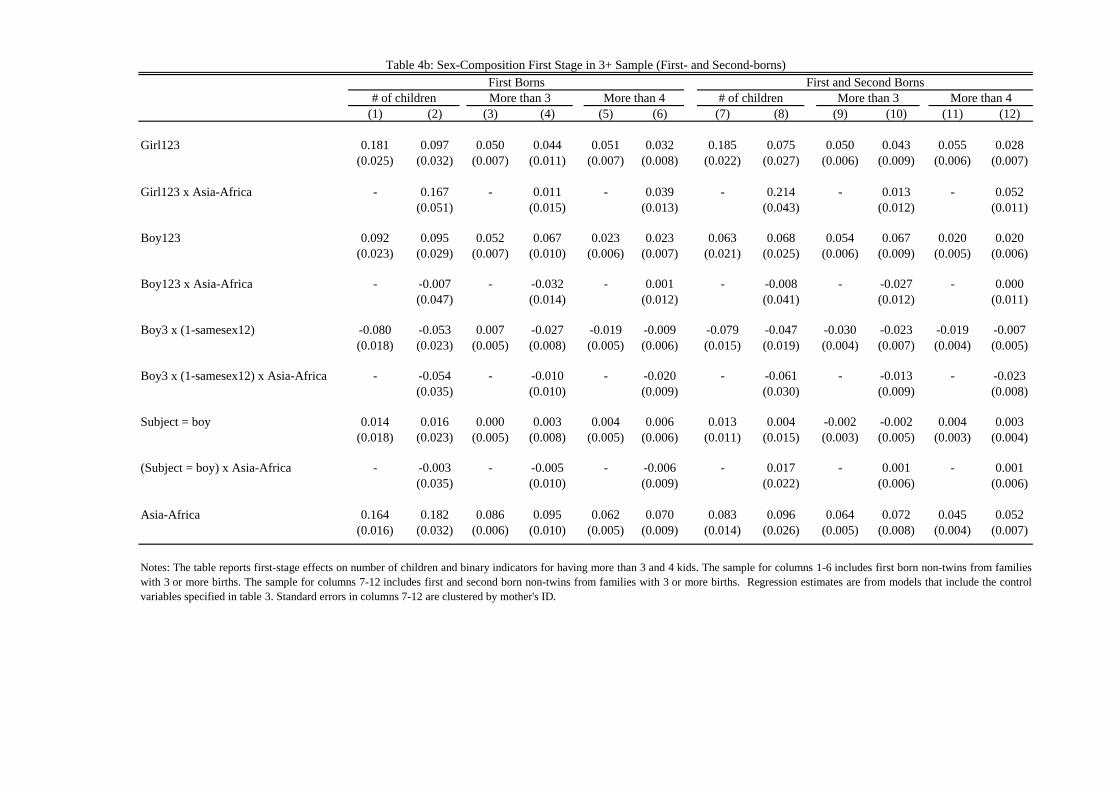
(1) (2) (3) (4) (5) (6) (7) (8) (9) (10) (11) (12)

Girl123 0.181 0.097 0.050 0.044 0.051 0.032 0.185 0.075 0.050 0.043 0.055 0.028(0.025) (0.032) (0.007) (0.011) (0.007) (0.008) (0.022) (0.027) (0.006) (0.009) (0.006) (0.007)

Girl123 x Asia-Africa - 0.167 - 0.011 - 0.039 - 0.214 - 0.013 - 0.052(0.051) (0.015) (0.013) (0.043) (0.012) (0.011)

Boy123 0.092 0.095 0.052 0.067 0.023 0.023 0.063 0.068 0.054 0.067 0.020 0.020(0.023) (0.029) (0.007) (0.010) (0.006) (0.007) (0.021) (0.025) (0.006) (0.009) (0.005) (0.006)

Boy123 x Asia-Africa - -0.007 - -0.032 - 0.001 - -0.008 - -0.027 - 0.000(0.047) (0.014) (0.012) (0.041) (0.012) (0.011)

Boy3 x (1-samesex12) -0.080 -0.053 0.007 -0.027 -0.019 -0.009 -0.079 -0.047 -0.030 -0.023 -0.019 -0.007(0.018) (0.023) (0.005) (0.008) (0.005) (0.006) (0.015) (0.019) (0.004) (0.007) (0.004) (0.005)

Boy3 x (1-samesex12) x Asia-Africa - -0.054 - -0.010 - -0.020 - -0.061 - -0.013 - -0.023(0.035) (0.010) (0.009) (0.030) (0.009) (0.008)

Subject = boy 0.014 0.016 0.000 0.003 0.004 0.006 0.013 0.004 -0.002 -0.002 0.004 0.003(0.018) (0.023) (0.005) (0.008) (0.005) (0.006) (0.011) (0.015) (0.003) (0.005) (0.003) (0.004)

(Subject = boy) x Asia-Africa - -0.003 - -0.005 - -0.006 - 0.017 - 0.001 - 0.001(0.035) (0.010) (0.009) (0.022) (0.006) (0.006)

Asia-Africa 0.164 0.182 0.086 0.095 0.062 0.070 0.083 0.096 0.064 0.072 0.045 0.052(0.016) (0.032) (0.006) (0.010) (0.005) (0.009) (0.014) (0.026) (0.005) (0.008) (0.004) (0.007)

Notes: The table reports first-stage effects on number of children and binary indicators for having more than 3 and 4 kids. The sample for columns 1-6 includes first born non-twins from familieswith 3 or more births. The sample for columns 7-12 includes first and second born non-twins from families with 3 or more births. Regression estimates are from models that include the controlvariables specified in table 3. Standard errors in columns 7-12 are clustered by mother's ID.

Table 4b: Sex-Composition First Stage in 3+ Sample (First- and Second-borns)

# of children More than 3 More than 4First Borns

# of children More than 3 More than 4First and Second Borns

Outcome (1) (2) (3) (4) (5) (6) (7) (8)Schooling

Highest grade completed 12.6 -0.252 -0.145 0.152 0.101 0.295 0.222 0.150(0.005) (0.005) (0.159) (0.130) (0.184) (0.176) (0.104)

Years of schooling ≥ 12 0.824 -0.037 -0.029 0.023 0.021 -0.009 -0.016 0.003(0.001) (0.001) (0.027) (0.021) (0.028) (0.028) (0.017)

Matriculation certificate 0.487 -0.054 -0.033 -0.009 -0.004 0.100 0.077 0.033(0.001) (0.001) (0.036) (0.033) (0.043) (0.040) (0.025)

Some College (age ≥ 24) 0.291 -0.049 -0.023 0.012 0.023 0.089 0.089 0.054(0.001) (0.001) (0.048) (0.045) (0.048) (0.046) (0.031)

College graduate (age ≥ 24) 0.202 -0.036 -0.015 -0.022 -0.008 0.115 0.115 0.052(0.001) (0.001) (0.041) (0.040) (0.046) (0.044) (0.028)

Labor Market Outcomes (age ≥ 22)Worked during the year 0.827 -0.025 -0.024 -0.011 0.000 0.063 0.072 0.032

(0.001) (0.001) (0.036) (0.032) (0.044) (0.043) (0.025)

Weekly labor force participation 0.817 -0.020 -0.020 0.006 0.003 0.018 0.033 0.015(0.001) (0.001) (0.038) (0.034) (0.043) (0.043) (0.026)

Hours worked last week 32.6 -1.06 -1.20 -0.76 -0.04 1.46 1.06 0.65(0.05) (0.06) (2.41) (2.14) (2.06) (1.98) (1.42)

Monthly earnings (in 1995 Shekels) 2,997 -217 -179 -6.76 55.5 266 430 261(7.4) (8.0) (362) (319) (283.8) (292) (209)

Ln(monthly earnings) 8.08 -0.034 -0.025 -0.032 0.007 -0.053 -0.067 -0.026(0.002) (0.002) (0.095) (0.085) (0.092) (0.083) (0.057)

MarriageMarried on census day 0.446 0.023 0.020 0.039 0.056 0.118 0.101 0.074

(0.001) (0.001) (0.028) (0.025) (0.034) (0.032) (0.019)

Married by age 21 (age ≥ 21) 0.172 0.027 0.022 -0.003 0.021 0.198 0.192 0.107(0.001) (0.001) (0.035) (0.031) (0.047) (0.046) (0.025)

Fertility (women only)Number of own children 1.00 0.123 0.110 0.182 0.037 0.191 0.178 0.115

(0.004) (0.004) (0.133) (0.086) (0.096) (0.097) (0.064)

Any children 0.448 0.126 0.019 0.093 0.012 0.136 0.134 0.078(0.001) (0.001) (0.057) (0.036) (0.041) (0.041) (0.026)

2 or more children 0.320 0.030 0.023 0.084 0.042 0.080 0.076 0.061(0.001) (0.001) (0.050) (0.032) (0.035) (0.036) (0.024)

Spouse's Outcomes (for married)Years of schooling 12.8 -0.325 -0.173 -0.274 -0.155 0.333 0.263 -0.002

(0.008) (0.009) (0.417) (0.324) (0.438) (0.421) (0.252)

Weekly labor force participation 0.848 -0.023 -0.023 -0.008 -0.012 0.033 0.035 0.011(0.001) (0.001) (0.052) (0.039) (0.040) (0.039) (0.028)

Monthly earnings (in 1995 Shekels) 3,241 -281 -223 112 -241 518 425 92.9(09) (10) (582) (437) (720) (658) (356)

Means

Table 5: Results for First Borns in 2+ Sample

Notes: The table reports means of the dependent variables (column 1) and coefficients on number of children for OLS models (columns 2-3) and 2SLSmodels using different sets of instruments (columns 4-8). Instruments with an ‘aa’ suffix are interaction terms with an AA dummy. The sample includesfirst borns from families with 2 or more births as decribed in Table 1. OLS estimates for column 2 include indicators for age and sex. Estimates forcolumns 3-8 are from models that include the control variables specified in Table 3. Robust standard errors are reported in parenthesis.

2SLS -- Instrument listgirl12, boy12,

girl12AA, boy12AA

girl12, boy12

twins, twinsAAtwins all

all covs.

basic covs.

OLS

Outcome (1) (2) (3) (4) (5) (6) (7) (8)Schooling

Highest grade completed -0.160 0.322 0.357 -0.099 -0.003 0.148 0.157 0.310(0.006) (0.176) (0.170) (0.166) (0.158) (0.114) (0.106) (0.149)

Years of schooling ≥ 12 -0.033 0.038 0.038 0.007 0.010 0.024 0.022 0.031(0.001) (0.027) (0.026) (0.027) (0.028) (0.019) (0.018) (0.024)

Matriculation certificate -0.038 0.082 0.093 -0.050 -0.018 0.028 0.038 0.087(0.001) (0.036) (0.036) (0.037) (0.034) (0.025) (0.023) (0.031)

Some College (age ≥ 24) -0.025 0.138 0.144 -0.044 -0.023 0.028 0.010 0.046(0.001) (0.059) (0.059) (0.036) (0.033) (0.028) (0.024) (0.037)

College graduate (age ≥ 24) -0.017 0.131 0.137 -0.072 -0.041 0.016 0.004 0.057(0.001) (0.052) (0.053) (0.034) (0.039) (0.025) (0.022) (0.034)

Labor Market Outcomes (age ≥ 22)Worked during the year -0.028 0.038 0.037 0.081 0.074 0.060 0.048 0.020

(0.001) (0.037) (0.036) (0.037) (0.036) (0.026) (0.023) (0.031)

Weekly labor force participation -0.024 0.033 0.034 0.023 0.013 0.022 0.017 0.020(0.001) (0.037) (0.037) (0.034) (0.033) (0.025) (0.022) (0.031)

Hours worked last week -1.44 2.72 2.69 3.40 3.36 3.29 2.28 1.09(0.06) (2.06) (2.05) (1.78) (1.70) (1.31) (1.16) (1.65)

Monthly earnings (in 1995 Shekels) -194 140 139 287 212 195 138 55(9.0) (327) (324) (253) (239) (198) (181) (275)

Ln(monthly earnings) -0.026 0.058 0.055 -0.014 0.001 0.028 0.005 0.009(0.003) (0.069) (0.070) (0.056) (0.051) (0.042) (0.039) (0.061)

MarriageMarried on census day 0.021 0.048 0.040 0.001 0.023 0.023 0.023 0.028

(0.001) (0.027) (0.027) (0.030) (0.028) (0.020) (0.018) (0.024)

Married by age 21 (age ≥ 21) 0.024 0.009 0.012 0.050 0.053 0.034 0.033 0.014(0.001) (0.031) (0.030) (0.034) (0.033) (0.022) (0.021) (0.027)

Fertility (women only)Number of own children 0.119 -0.154 -0.160 -0.129 -0.103 -0.127 -0.125 -0.157

(0.006) (0.089) (0.084) (0.094) (0.089) (0.063) (0.058) (0.081)

Any children 0.022 0.014 0.008 0.006 0.023 0.017 0.023 0.011(0.002) (0.038) (0.037) (0.033) (0.031) (0.024) (0.021) (0.031)

2 or more children 0.025 -0.012 -0.011 -0.001 0.010 0.001 -0.006 -0.030(0.002) (0.037) (0.035) (0.031) (0.030) (0.023) (0.021) (0.030)

3 or more children 0.026 -0.085 -0.082 -0.069 -0.066 -0.073 -0.068 -0.062(0.002) (0.027) (0.026) (0.031) (0.030) (0.021) (0.019) (0.025)

Spouse's Outcomes (for married)Years of schooling -0.180 1.00 1.00 -0.379 -0.267 0.181 0.126 0.581

(0.010) (0.56) (0.55) (0.283) (0.266) (0.238) (0.213) (0.362)

Weekly labor force participation -0.025 0.106 0.105 0.044 0.038 0.056 0.038 0.038(0.001) (0.059) (0.059) (0.032) (0.030) (0.026) (0.023) (0.038)

Monthly earnings (in 1995 Shekels) -241 585 565 -612 -400 -99.0 -118 162(11) (565) (558) (536) (473) (346) (303) (396)

all, boy3, boy3AA

2SLS -- Instrument listtwins,

twinsAA, boy3,

boy3AA

Table 6a: Results for First Borns in 3+ Sample

Notes: The table reports coefficients on number of children for OLS models (column 1) and 2SLS models using different sets of instruments (columns 2-8).Instruments with an ‘aa’ suffix are interaction terms with an AA dummy. The sample includes first borns from families with 3 or more births as decribed in Table 1.Regression estimates are from models that include the control variables specified in Table 3. Robust standard errors are reported in parenthesis.

allOLS

all covs. twins

girl123, boy123,

girl123AA, boy123AA

twins, twinsAA

girl123, boy123

Outcome (1) (2) (3) (4) (5) (6) (7) (8)Schooling

Highest grade completed -0.143 0.167 0.187 -0.108 -0.054 0.076 0.080 0.175(0.005) (0.119) (0.111) (0.134) (0.120) (0.081) (0.077) (0.101)

Years of schooling ≥ 12 -0.031 0.025 0.025 0.001 -0.007 0.016 0.012 0.017(0.001) (0.019) (0.018) (0.023) (0.022) (0.014) (0.013) (0.017)

Matriculation certificate -0.033 0.057 0.065 -0.019 0.008 0.036 0.042 0.069(0.001) (0.026) (0.026) (0.030) (0.027) (0.019) (0.018) (0.023)

Some College (age ≥ 24) -0.021 0.061 0.062 -0.047 -0.022 0.010 0.002 0.024(0.001) (0.037) (0.036) (0.030) (0.025) (0.021) (0.018) (0.027)

College graduate (age ≥ 24) -0.015 0.065 0.068 -0.056 -0.031 0.003 -0.001 0.037(0.001) (0.036) (0.037) (0.026) (0.022) (0.019) (0.016) (0.024)

Labor Market Outcomes (age ≥ 22)Worked during the year -0.027 0.029 0.034 0.038 0.035 0.037 0.039 0.043

(0.001) (0.025) (0.024) (0.029) (0.027) (0.018) (0.017) (0.021)

Weekly labor force participation -0.023 0.028 0.035 -0.001 -0.006 0.011 0.018 0.040(0.001) (0.025) (0.024) (0.028) (0.026) (0.018) (0.016) (0.021)

Hours worked last week -1.41 2.38 2.53 1.44 1.56 2.29 2.11 2.59(0.05) (1.48) (1.45) (1.36) (1.28) (0.97) (0.89) (1.26)

Monthly earnings (in 1995 Shekels) -185 46.6 63.4 127 115 103 107 96(6.77) (207) (206) (176) (162) (131) (122) (180)

Ln(monthly earnings) -0.027 0.017 0.011 0.013 0.031 0.038 0.019 0.005(0.002) (0.048) (0.049) (0.050) (0.046) (0.033) (0.031) (0.042)

MarriageMarried on census day 0.020 0.022 0.016 0.019 0.041 0.022 0.015 0.006

(0.001) (0.018) (0.018) (0.024) (0.022) (0.014) (0.013) (0.016)

Married by age 21 (age ≥ 21) 0.024 0.029 0.027 0.044 0.050 0.039 0.035 0.018(0.001) (0.021) (0.023) (0.031) (0.030) (0.019) (0.017) (0.019)

Fertility (women only)Number of own children 0.118 -0.069 -0.077 -0.079 -0.043 -0.058 -0.076 -0.097

(0.004) (0.066) (0.061) (0.069) (0.064) (0.045) (0.043) (0.059)

Any children 0.023 0.020 0.014 -0.003 0.012 0.013 0.010 0.006(0.001) (0.029) (0.028) (0.025) (0.022) (0.017) (0.016) (0.025)

2 or more children 0.025 -0.002 -0.005 -0.007 0.007 0.002 -0.005 -0.016(0.001) (0.026) (0.024) (0.023) (0.021) (0.016) (0.015) (0.022)

3 or more children 0.026 -0.050 -0.047 -0.042 -0.037 -0.041 -0.041 -0.037(0.001) (0.020) (0.019) (0.021) (0.020) (0.014) (0.013) (0.018)

Spouse's Outcomes (for married)Years of schooling -0.166 0.539 0.552 -0.325 -0.233 0.106 0.095 0.389

(0.008) (0.308) (0.294) (0.225) (0.201) (0.162) (0.145) (0.218)

Weekly labor force participation -0.023 0.043 0.037 0.026 0.010 0.020 0.012 0.014(0.001) (0.034) (0.033) (0.024) (0.020) (0.017) (0.016) (0.024)

Monthly earnings (in 1995 Shekels) -217 429 426 -889 -442 -151 -250 -77(9.0) (350) (345) (414) (322) (230) (202) (253)

Table 6b: Results for First and Second Borns in 3+ Sample 2SLS -- Instrument list

Notes: The table reports coefficients on number of children for OLS models (column 1) and 2SLS models using different sets of instruments (columns 2-8). Instrumentswith an ‘aa’ suffix are interaction terms with an AA dummy. The sample includes first and second borns from families with 3 or more births as decribed in Table 1.Regression estimates are from models that include the control variables specified in Table 3. Standard errors are clustered by mother's ID.

twins, twinsAA,

boy3, boy3AA

OLSall covs. twins

twins, twinsAA

girl123, boy123

girl123, boy123,

girl123AA, boy123AA all

all, boy3, boy3AA

1st borns 1st+2nd 1st borns 1st+2nd

OLS 2SLS 2SLS 2SLS OLS 2SLS 2SLS 2SLSOutcome (1) (2) (3) (4) (5) (6) (7) (8)Schooling

Highest grade completed -0.156 0.189 0.240 0.202 -0.134 0.108 0.076 -0.013(0.008) (0.119) (0.156) (0.116) (0.007) (0.207) (0.139) (0.101)

Years of schooling ≥ 12 -0.031 0.013 0.013 0.028 -0.025 -0.015 0.020 -0.009(0.001) (0.019) (0.024) (0.019) (0.001) (0.036) (0.025) (0.018)

Matriculation certificate -0.042 0.038 0.072 0.069 -0.028 0.022 0.012 0.027(0.002) (0.030) (0.037) (0.029) (0.001) (0.045) (0.028) (0.022)

Some College (age ≥ 24) -0.039 0.063 0.012 0.010 -0.018 0.054 0.014 -0.002(0.002) (0.038) (0.052) (0.038) (0.001) (0.047) (0.027) (0.020)

College graduate (age ≥ 24) -0.026 0.060 0.006 0.006 -0.012 0.053 0.004 -0.006(0.002) (0.034) (0.049) (0.035) (0.001) (0.041) (0.023) (0.017)

Labor Market Outcomes (age ≥ 22)Worked during the year -0.038 0.015 0.077 0.080 -0.016 0.061 0.030 0.017

(0.002) (0.029) (0.038) (0.028) (0.001) (0.048) (0.028) (0.021)

Weekly labor force participation -0.035 0.002 0.093 0.091 -0.012 0.043 -0.020 -0.015(0.002) (0.030) (0.039) (0.029) (0.001) (0.048) (0.027) (0.021)

Hours worked last week -2.08 0.01 4.28 4.27 -0.73 1.02 1.03 0.69(0.09) (1.72) (2.17) (1.68) (0.07) (2.34) (1.34) (1.05)

Monthly earnings (in 1995 Shekels) -262 369 345 330 -132 87 30 -8(13) (273) (347) (257) (10) (293) (208) (138)

Ln(monthly earnings) -0.033 0.057 -0.006 -0.001 -0.022 -0.190 0.006 0.014(0.005) (0.073) (0.075) (0.056) (0.003) (0.101) (0.044) (0.036)

MarriageMarried on census day 0.034 0.088 -0.013 -0.009 0.010 0.046 0.052 0.037

(0.001) (0.022) (0.027) (0.021) (0.001) (0.038) (0.024) (0.018)

Married by age 21 (age ≥ 21) 0.040 0.085 0.017 0.012 0.015 0.140 0.046 0.047(0.002) (0.028) (0.032) (0.024) (0.001) (0.054) (0.028) (0.022)

Fertility (women only)Number of own children 0.148 0.120 -0.189 -0.130 0.088 0.130 -0.093 -0.054

(0.008) (0.074) (0.088) (0.065) (0.006) (0.116) (0.075) (0.056)

Any children 0.030 0.063 -0.019 -0.011 0.015 0.130 0.043 0.020(0.002) (0.032) (0.038) (0.029) (0.002) (0.116) (0.027) (0.021)

2 or more children 0.032 0.064 -0.013 -0.024 0.018 0.115 -0.004 0.001(0.002) (0.028) (0.035) (0.025) (0.002) (0.047) (0.026) (0.019)

3 or more children 0.032 0.008 -0.070 -0.044 0.021 0.062 -0.065 -0.040(0.002) (0.021) (0.028) (0.019) (0.002) (0.042) (0.024) (0.018)

Spouse's Outcomes (for married)Years of schooling -0.213 0.112 0.050 0.129 -0.156 -0.150 -0.002 -0.046

(0.014) (0.301) (0.388) (0.275) (0.011) (0.439) (0.239) (0.168)

Weekly labor force participation -0.039 -0.012 -0.010 -0.019 -0.013 0.038 0.047 0.016(0.002) (0.035) (0.048) (0.034) (0.002) (0.042) (0.027) (0.018)

Monthly earnings (in 1995 Shekels) -331 -76 10 -187 -163 274 -211 -300(17) (433) (635) (407) (13) (665) (329) (241)

Notes: The table reports OLS and 2SLS results estimated separately by ethnicity.The 2SLS estimates are from models that include the full set of instruments(i.e. corresponding to column 8 in table 5 and column 7 in tables 6a and 6b). Regression estimates are from models that include the control variablesspecified in Table 3. Robust standard errors are reported in parenthesis. Standard errors for columns 4 and 8 are clustered by mother's ID.

Table 7: Full Specification By Ethnicity

3+2+1st borns

2+1st borns

Asia/AfricaIsrael/Europe3+

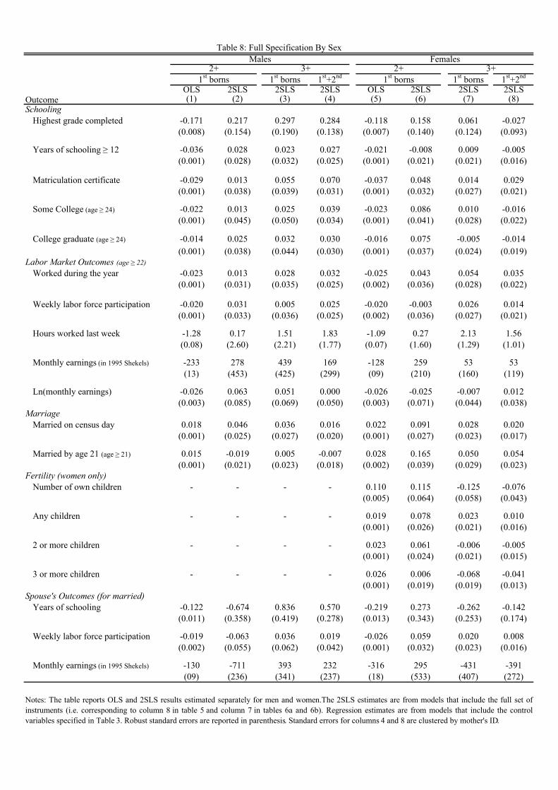
1st borns 1st+2nd 1st borns 1st+2nd

OLS 2SLS 2SLS 2SLS OLS 2SLS 2SLS 2SLSOutcome (1) (2) (3) (4) (5) (6) (7) (8)Schooling

Highest grade completed -0.171 0.217 0.297 0.284 -0.118 0.158 0.061 -0.027(0.008) (0.154) (0.190) (0.138) (0.007) (0.140) (0.124) (0.093)

Years of schooling ≥ 12 -0.036 0.028 0.023 0.027 -0.021 -0.008 0.009 -0.005(0.001) (0.028) (0.032) (0.025) (0.001) (0.021) (0.021) (0.016)

Matriculation certificate -0.029 0.013 0.055 0.070 -0.037 0.048 0.014 0.029(0.001) (0.038) (0.039) (0.031) (0.001) (0.032) (0.027) (0.021)

Some College (age ≥ 24) -0.022 0.013 0.025 0.039 -0.023 0.086 0.010 -0.016(0.001) (0.045) (0.050) (0.034) (0.001) (0.041) (0.028) (0.022)

College graduate (age ≥ 24) -0.014 0.025 0.032 0.030 -0.016 0.075 -0.005 -0.014(0.001) (0.038) (0.044) (0.030) (0.001) (0.037) (0.024) (0.019)

Labor Market Outcomes (age ≥ 22)Worked during the year -0.023 0.013 0.028 0.032 -0.025 0.043 0.054 0.035

(0.001) (0.031) (0.035) (0.025) (0.002) (0.036) (0.028) (0.022)

Weekly labor force participation -0.020 0.031 0.005 0.025 -0.020 -0.003 0.026 0.014(0.001) (0.033) (0.036) (0.025) (0.002) (0.036) (0.027) (0.021)

Hours worked last week -1.28 0.17 1.51 1.83 -1.09 0.27 2.13 1.56(0.08) (2.60) (2.21) (1.77) (0.07) (1.60) (1.29) (1.01)

Monthly earnings (in 1995 Shekels) -233 278 439 169 -128 259 53 53(13) (453) (425) (299) (09) (210) (160) (119)

Ln(monthly earnings) -0.026 0.063 0.051 0.000 -0.026 -0.025 -0.007 0.012(0.003) (0.085) (0.069) (0.050) (0.003) (0.071) (0.044) (0.038)

MarriageMarried on census day 0.018 0.046 0.036 0.016 0.022 0.091 0.028 0.020

(0.001) (0.025) (0.027) (0.020) (0.001) (0.027) (0.023) (0.017)

Married by age 21 (age ≥ 21) 0.015 -0.019 0.005 -0.007 0.028 0.165 0.050 0.054(0.001) (0.021) (0.023) (0.018) (0.002) (0.039) (0.029) (0.023)

Fertility (women only)Number of own children - - - - 0.110 0.115 -0.125 -0.076

(0.005) (0.064) (0.058) (0.043)

Any children - - - - 0.019 0.078 0.023 0.010(0.001) (0.026) (0.021) (0.016)

2 or more children - - - - 0.023 0.061 -0.006 -0.005(0.001) (0.024) (0.021) (0.015)

3 or more children - - - - 0.026 0.006 -0.068 -0.041(0.001) (0.019) (0.019) (0.013)

Spouse's Outcomes (for married)Years of schooling -0.122 -0.674 0.836 0.570 -0.219 0.273 -0.262 -0.142

(0.011) (0.358) (0.419) (0.278) (0.013) (0.343) (0.253) (0.174)

Weekly labor force participation -0.019 -0.063 0.036 0.019 -0.026 0.059 0.020 0.008(0.002) (0.055) (0.062) (0.042) (0.001) (0.032) (0.023) (0.016)

Monthly earnings (in 1995 Shekels) -130 -711 393 232 -316 295 -431 -391(09) (236) (341) (237) (18) (533) (407) (272)

Notes: The table reports OLS and 2SLS results estimated separately for men and women.The 2SLS estimates are from models that include the full set ofinstruments (i.e. corresponding to column 8 in table 5 and column 7 in tables 6a and 6b). Regression estimates are from models that include the controlvariables specified in Table 3. Robust standard errors are reported in parenthesis. Standard errors for columns 4 and 8 are clustered by mother's ID.

Table 8: Full Specification By Sex

1st borns2+

1st borns

FemalesMales3+ 2+ 3+

Figure 1: First-borns 2+ sample. First stage effects by ethnicity and type of sex-mix.

Asia-Africa: Girl12=1

-0.02

-0.01

0.00

0.01

0.02

0.03

0.04

0.05

0.06

0.07

3+ 4+ 5+ 6+ 7+ 8+ 9+ 10+

Number of children

Total: 0.138 (0.029)

Israel/Europe: Boy12=1

-0.02

-0.01

0.00

0.01

0.02

0.03

0.04

0.05

0.06

0.07

3+ 4+ 5+ 6+ 7+ 8+ 9+ 10+

Number of children

Total: 0.078 (0.017)

Israel/Europe: Girl12=1

-0.02

-0.01

0.00

0.01

0.02

0.03

0.04

0.05

0.06

0.07

3+ 4+ 5+ 6+ 7+ 8+ 9+ 10+

Number of children

Total: 0.098 (0.018)

Asia-Africa: Boy12=1

-0.02

-0.01

0.00

0.01

0.02

0.03

0.04

0.05

0.06

0.07

3+ 4+ 5+ 6+ 7+ 8+ 9+ 10+

Number of children

Total: 0.013 (0.028)

Figure 2: First borns 3+ sample. First stage effects by ethnicity and type of sex-mix (conditional on samesex12=1).

Asia-Africa: Girl123=1

-0.02

-0.01

0.00

0.01

0.02

0.03

0.04

0.05

0.06

0.07

0.08

0.09

0.10

4+ 5+ 6+ 7+ 8+ 9+ 10+ 11+

Number of children

Total: 0.292 (0.042)

Israel/Europe: Boy123=1

-0.02

-0.01

0.00

0.01

0.02

0.03

0.04

0.05

0.06

0.07

0.08

0.09

0.10

4+ 5+ 6+ 7+ 8+ 9+ 10+ 11+

Number of children

Total: 0.088 (0.030)

Israel/Europe: Girl123=1

-0.02

-0.01

0.00

0.01

0.02

0.03

0.04

0.05

0.06

0.07

0.08

0.09

0.10

4+ 5+ 6+ 7+ 8+ 9+ 10+ 11+

Number of children

Total: 0.084 (0.033)

Asia-Africa: Boy123=1

-0.02

-0.01

0.00

0.01

0.02

0.03

0.04

0.05

0.06

0.07

0.08

0.09

0.10

4+ 5+ 6+ 7+ 8+ 9+ 10+ 11+

Number of children

Total: 0.080 (0.040)

Figure 3: First borns 3+ sample. First stage effects of Boy3 (conditional on samesex12=0)

Asia/Africa: Boy3=1

-0.05

-0.04

-0.03

-0.02

-0.01

0.00

0.01

4+ 5+ 6+ 7+ 8+ 9+ 10+ 11+

Number of children

Israel/Europe: Boy3=1

-0.05

-0.04

-0.03

-0.02

-0.01

0.00

0.01

4+ 5+ 6+ 7+ 8+ 9+ 10+ 11+

Number of children

Total: -0.113 (0.029) Total: -0.026 (0.023)

2+1st borns 1st borns 1st and 2nd borns

(1) (2) (3)

Twins 0.640 0.602 0.711(0.057) (0.048) (0.054)

Twins x Asia-Africa -0.443 -0.109 -0.199(0.106) (0.100) (0.094)

Girls 0.090 0.102 0.082(0.017) (0.032) (0.027)

Girls x Asia-Africa 0.053 0.166 0.210(0.032) (0.051) (0.043)

Boys 0.061 0.103 0.075(0.017) (0.029) (0.025)

Boys x Asia-Africa -0.045 -0.014 -0.146(0.030) (0.047) (0.040)

Boy3 x (1-samesex12) - -0.049 -0.041(0.023) (0.019)

Boy3 x (1-samesex12) x Asia-Africa - -0.057 -0.065(0.035) (0.030)

Subect = boy 0.012 0.018 0.005(0.017) (0.023) (0.149)

(Subject = boy) x Asia-Africa 0.007 -0.005 0.016(0.031) (0.035) (0.223)

Asia-Africa 0.242 0.190 0.103(0.024) (0.032) (0.025)

3+Table A1: Pooled First Stage

Notes: The table reports first-stage effects on number of children using the full set of instruments.The regression estimates are from models that include the control variables specified in Table 3.Robust standard errors are reported in parenthesis. Standard errors in column 3 are clustered bymother's ID.