NBER WORKING PAPER SERIES

MONETARY POLICY WITH FLEXIBLEEXCHANGE RATES AND FORWARDINTEREST RATES AS INDICATORS

Lars E. 0. Svensson

Working Paper No. 4633

NATIONAL BUREAU OF ECONOMIC RESEARCH1050 Massachusetts Avenue

Cambridge, MA 02138January 1994

Presented at the 13th Bank of France-University Conference, "Capital Movements andExchange Rate Politics," November 24-26, 1993, and to be published in CahiersEconomiqueset Monétaires. I thank the discussant Jean-Pierre Laffargue and conference participants forcomments. I also thank Rod Beetsma, Magnus Dahiquist, Jon Faust, Mark Fisher, LanHorngren, Assar Lindbeck, Hans Lindberg, Maurice Obstfeld, Vincent Reinhart, AndersVredin, David Zervos, and participants in a seminar at the Stockholm School of Economicsfor discussions and comments on a previous version; Marten Blix and Joaidm Persson forresearch assistance; and Molly Akerlund and Patricia Reinhold for secretarial and editorialassistance. This paper is part of NBER's research programs in International Finance andMacroeconomics and Monetary Economics. Any opinions expressed axe those of the authorand not those of the National Bureau of Economic Research.

NBER Working Paper #4633January 1994

MONETARY POLICY WITH FLEXIBLEEXCHANGE RATES AND FORWARDINTEREST RATES AS Th4DICATORS

ABSTRACT

In the new situation with flexible exchange rates, monetary policy in Europe will have

to rely more on indicators than previously under fixed rates. One of the potential indicators, the

forward interest rate curve, can be used to indicate market expectations of the time-paths of

future short interest rates, monetary policy, inflation rates and currency depreciation rates. The

forward rate curve separates market expectations for the short, medium and long term more easily

than the standard yield curve. Monetary policy in France, Germany, Great Britain, Sweden and

the United States is interpreted with the help of forward rates.

Lars E. 0. SvenssonInstitute for international Economic StudiesStockholm University10691 StockholmSWEDENCEPR and NBER

1. Introduction

Previous monetary policy with fixed exchange rates in Europe the last few years can

be described, with some simplification, as Germany's pursuing an independent monetarypolicy directed as domestic price stability, and the rest of the countries' pegging their

exchange rate to the German mark, the European anchor currency. This was the case for

the countries within the ERM as well as the countries outside the ERM that unilaterally

pegged their exchange rate to the mark, as Austria, or the ecu, as Finland, Norway and

Sweden. Monetary policy outside Germany was then in principle very simple, it consisted

solely in defending a fixed exchange rate towards the mark or the ecu. This in turn, again

with some simplification, implied that central banks had to set interest rates so as to

roughly balance capital flows.The last year's turmoil in Europe has dramatically changed this. The Finnish markka,

the Italian lira and the British pound were forced to float in September 1992. In November

the same year the Swedish krona was floated, in December the Norwegian krone. InAugust 1993 the exchange rate bands for the currencies that remained in the ERM were

increased to percent, with the exception of the German mark and the Dutch guilder

which remained in the narrow band.The loss of the fixed exchange rates means the loss of the nominal anchor for the

countries that used to peg their exchange rates to the mark or the ecu. Except forAustria and the Netherlands, fixed exchange rates do not now seem, a realistic alternative

for the European countries in the short or medium term. Even if fixed exchange ratestowards a stable currency were feasible, if the ultimate target for monetary policy is price

stability, one can seriously doubt the efficiency of fixed exchange rates as an intermediate

target to achieve price stability (see Svensson (1994)). Hence, for several reasons there

is a need to discuss how monetary policy should he designed in the new situation with

flexible exchange rates in Europe.

This paper briefly discusses the design of monetary policy with flexible exchange rates,

in terms of the convenient and generally accepted conceptual framework of goals, inter-

mediate targets, indicators and instruments of monetary policy. It argues that likelydifficulties in finding appropriate intermediate targets will increase the role of indicators

for assessing the state of the economy, the stance of monetary policy, and how the in-

struments should be adjusted to achieve the goal of monetary policy. Several indicators

wifl have to be used simultaneously. The paper extends on the use of one of the possi-

ble indicators, the forward interest rate, and discusses how forward interest rates can be

I

used to extract market expectations of future interest rate, inflation rates and currencydepreciation rates. Some discussion and interpretation of forward interest rates in France,

Germany, Great Britain, Sweden and the United States is provided)The paper is outlined as follows. Section 2 discusses the design of monetary policy

with flexible exchange rates in terms of the conceptual framework of goals, intermediate

targets, indicators and instruments. Section 3 provides definitions of yields to maturity,

zero-coupon interest rates (spot rates) and forward interest rates. Sections 4, 5 and 6discusses how forward interest rates can be used to extract expected future interestrates,expected future inflation, and expected future currency depreciation, respectively. Three

different risk premia (term, inflation, and foreign exchange risk premia) are defined anddiscussed. Section 7 provides a comparison and discussion of forward interest rates inFrance, Germany, Great Britain, Sweden and the United States. Section 8 concludes.Appendix A reports on the estimation of forward rates from bond yields, and AppendixB defines three related concepts of term prernia.

2. Monetary Policy with Flexible Exchange Rates

A generally accepted conceptual framework for the design of monetary policy distinguishesbetween goals, intermediate targets, indicators and instruments (see Friedman (1990) orMcCallum (1990), for example).2 As the term implies, the goals ofmonetary policy—pricestability and full employment, for example—are the ultimate objectives ofmonetary policy.Monetary policy is complicated by the fact that the central bank has only very indirectcontrol over the variables that usually constitute the goals. These variablesreact with longand variable lags to monetary policy. The variables themselves are observed with some-times rather substantial delays, at rather long intervals, and with substantial statisticaluncertainty. Some central banks select intermediate targets such as variousmoney-supplyaggregates or the exchange rate. These intermediate targets do not necessarily haveanyintrinsic value, apart from their correlation with the goals. They are more controllableand more readily observed than the goals (they are observed more often, with less timelag, and react more quickly to monetary policy). Properly chosen intermediate targetscan therefore contribute to fulfilling the goals. Indicators are variables that provide the

'Forward interest rates are already used as one of themonetary policy indicators by Bank of England,Board of Governors of the Federal Reserve System, and Sveriges Rikshank. Their role as indicators isdiscussed in Bank of England (1993b), Svensson (1993a) and Sveriges Riksbank (1993). See also Bankfor International Settlements (1993, p. 144).

2This section builds to some extent upon Svensson (1992).

2

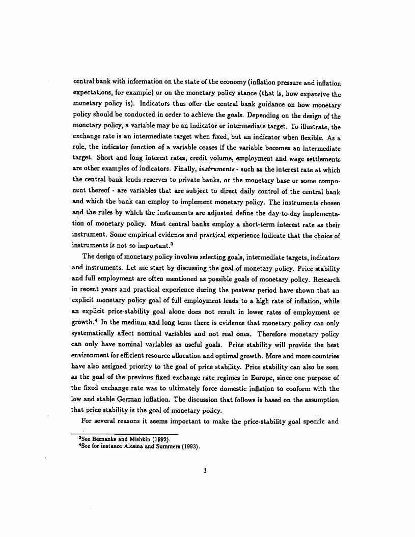
central bank with information on the state of the economy (inflation pressure and inflation

expectations, for example) or on the monetary policy stance (that is, how expansive themonetary policy is). Indicators thus offer the central bank guidance on how monetarypolicy should be conducted in order to achieve the goals. Depending on the design of the

monetary policy, a variable may be an indicator or intermediate target. To illustrate, the

exchange rate is an intermediate target when fixed, but an indicator when flexible. As arule, the indicator function of a variable ceases if the variable becomes an intermediate

target. Short and long interest rates, credit volume, employment and wage settlementsare other examples of indicators. Finally, instruments- such as the interest rate at which

the central bank lends reserves to private banks, or the monetary base or somecompo-nent thereof - are variables that are subject to direct daily control of the central bankand which the bank can employ to implement monetary policy. The instruments chosenand the rules by which the instruments are adjusted define the day-to-day implementa-

tion of monetary policy. Most central banks employ a short-term interest rate as their

instrument. Some empirical evidence and practical experience indicate that the choice ofinstruments is not so important.3

The design of monetary policy involves selecting goals, intermediate targets, indicators

and instruments. Let me start by discussing the goal of monetary policy. Price stabilityand full employment are often mentioned as possible goals of monetary policy. Research

in recent years and practical experience during the postwar period have shown that anexplicit monetary policy goal of full employment leads to a high rate of inflation, while

an explicit price-stability goal alone does not result in lower rates of employment orgrowth.4 In the medium and long term there is evidence that monetary policy can only

systematically affect nominal variables and not real ones. Therefore monetary policycan only have nominal variables as useful goals. Price stability will provide the bestenvironment for efficient resource allocation and optimal growth. More and more countries

have also assigned priority to the goal of price stability. Price stability can also be seenas the goal of the previous fixed exchange rate regimes in Europe, since one purpose of

the fixed exchange rate was to ultimately force domestic inflation to conform with the

low and stable German inflation. The discussion that follows is based on the assumption

that price stability is the goal of monetary policy.For several reasons it seems important to make the price-stability goal specific and

3See Bernanke and Mishkin (1992).4See for instance Alesina and Summers (1993).

3

precise. A precisely defined goal may reduce the uncertainty about monetary policy thata forced switch to a flexible exchange rate in all likelihood has caused. A precisely defined

goal means a stronger commitment to monetary policy and can increase its credibility. A

precisely defined goal makes it possible to monitor how well the goal is being met and to

criticize the central bank directly, even holding it responsible, in the event thegoal is notmet. A precisely defined goal can also help to stabilize inflation expectations.

Against this background, it seems suitable to define price stability as an interval for thefuture price level or its rate of change, where the price level in turn is defined by the mostcommonly known price index, the consumer price index. Several countries haverecentlyspecified explicit inflation targets, for instance Britain, Finland and Sweden, followingearlier examples of Canada and New Zealand. (See Freedman (1993) for a discussion ofthe Canadian experience of inflation targets, and for references to the relevant literature.)

Both theory and practical experiences indicate that institutional reform can enhancethe credibility of the price-stability goals by: establishing price stability as the goal ofmonetary policy; by giving the central bank the independence that will enable it to achievethe goal and resist short-term pressures and special interestgroups; and by holding theBoard of Governors and management of the central bank accountable if thegoal is notmet.

Although there is evidence that monetary policy in the medium and long term can sys-tematically affect only nominal variables, there is certainly evidence that monetary policyhas effects on real variables, output and employment, in the shortrun. Therefore, mone-tary policy may stabilize or destabilize short-run fluctuations inoutput and employment,although it cannot systematically affect average output and employment in the mediumand long run. This fact is not an argument against price stability as a goal for monetarypolicy. On the contrary, a credible price-stability goal is likely to make monetary policymore effective in stabilizing short-run output fluctuations, for two reason.

First, a price-stability policy implies an automatic stabilization ofaggregate demandshocks. An increase in aggregate demand that leads to increased inflation will be metwith a monetary contraction; vice versa for a decrease in aggregate demand. Second, it islikely that long-run credibility for a price-stability policygives central bank more discre-tion to stabilize output in the short run, as discussed in Bernanke and Mishkin (l992).Without such long-run credibility a short-run monetary expansion may be interpreted bythe private sector as the beginning of an extended period of monetary expansion. There-

5See also Hörngren and Lindberg (1993).

4

fore it may result in increased inflation expectations and increased wages, prices andlong-term interest rates. This may both dampen the initial stimulating effect on output

and lock the economy into a situation with high inflation. With long-run credibility, ashort-run monetary expansion rate will not lead to increased inflation expectations and

their accompanying negative effects.As examples of this, Germany and the United States seem to have established good

long-mn credibility for a price-stability policy, with low long interest rates and low long-

run inflation expectations. This should imply considerable discretion in the short-run.

Consistent with this, the United States has been able to meet the latest recession with a

very expansionary monetary policy with very low short-term real interest, rates, withoutany rise in long-run inflation expectations and long-term interest rates. Britain and Swe-

den, in contrast, seem to have lower long-run credibility for their price-stability policy,which shows up in higher long-term interest rates and higher long-run inflation expec-tations. Monetary expansion after the pound and the krona were floated indeed seem

to have resulted in increased inflation expectations, as will be further discussed below in

section 7. The scope for short-run monetary policy to stabilize output without endanger-

ing price stability seems smaller in Britain and Sweden than in German and the United

States.After this discussion of the goal of monetary policy, let me go on to discuss interme-

diate targets. Since the central bank has only indirect control over the price level, andsince the latter reacts with "long and variable lags" to monetary policy measures, it may

be desirable to select an intermediate target. An ideal intermediate target has a highcorrelation with the goal but is much easier to control and monitor. Thus, monetarypolicy is made easier if it is focused on the intermediate target. It is easy to monitor how

well the central bank meets the intermediate target and the bank can more readily be

held accountable if the intermediate target is not met. But the problem, not surprisingly,

is that it is difficult to find an ideal intermediate target.A fixed exchange rate towards a currency with a low and stable inflation can be seen

as an intermediate target to achieve price stability. However, fixed exchange rates do not

seem a realistic possibility in Europe in the short or medium term, except for Austriaand the Netherlands. Even if fixed exchange rates against a stable currency were feasible,

they may be a rather inefficient means to price stability, as argued in Svensson (1994).

Various money supply aggregates (from the monetary base to M3) are common as

intermediate targets. In the academic literature, such broader aggregates as nominal

5

expenditure and nominal GDP have also been proposed as intermediate targets.6 Here,

however, there is a conflict; although more narrow money-supply aggregates are easier

to control, they may be very weakly correlated with the goal, while broader aggregatescorrelate more closely with the goal but are more difficult to control. A special problem is

the fact that money supply aggregates have in many cases exhibited great instability-inconnection with financial innovations or changes in credit market regulations, for example.

Many observers have considered Germany's use of M3 as an intermediate target amodel for other countries.7 A target for the annual change in M3 is calculated based

on forecasts of the annual change in velocity and potential GNP, and on an explicitinflation goal. However, this procedure requires stable empirical estimates of demand for

money and experience in forecasting the velocity. In the short term it may be difficult to

judge whether velocities are sufficiently forecastable for monetary aggregates to serve as

intermediate targets.8 One particular problem is that the change from a fixed exchangerate to a flexible rate may itself affect the demand for money, in which case estimates with

data from the period with a fixed exchange rate will no longer be applicable. At least inthe short term after the abandonment of the fixed exchange rates, it seems most likely

that monetary aggregates will be important indicators but not intermediatetargets.This implies a very important role for indicators. Without an intermediate target, only

indicators remain between the instrument and the goal. The central bank will then haveto use available indicators to assess the state of the economy and the stance of monetary

policy in order to decide whether the instrument need to be adjusted or not for achieving

price stability.

The central bank will need indicators of inflation pressure, especially indicators thatforecast inflation one to two years ahead, since this is probably about the lag betweenthe price level and monetary policy measures. A number of indicators willobviously be

necessary for this, including money and credit aggregates, output gaps, vacancies andunemployment, asset prices and a number of other indicators used in forecasting businesscycles.

Indicators of inflation expectations will be of great interest rates, for at least tworear

'See Friedman (1990), McCallum (1990) and Rogoff (1985).TSee Bernazike and Mishkin (1992).'It is worth noting that Germany's financial mazket is less developed than many other countries

and that Gennany lacks alternatives to bank deposits for interest-basedsavings by households and smallcompanies. This contributes to the relatively stability o(the demand for money, which can be expected toexceed that in many other countries where private bonds, National Debt Office accounts, money-marketfunds and other instruments have already been introduced.

6

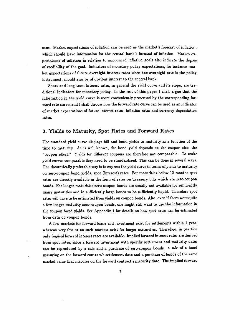
sons. Market expectations of inflation can be seen as the market's forecast of inflation,

which should have information for the central bank's forecast of inflation. Market ex-

pectations of inflation in relation to announced inflation goals also indicate the degree

of credibility of the goal. Indicators of monetary policy expectations, for instance mar-ket expectations of future overnight interest rates when the overnight rate is the policyinstrument, should also be of obvious interest to the central bank.

Short and long term interest rates, in general the yield curve and its slope, are tra-ditional indicators for monetary policy. in the rest of this paper I shall argue that the

information in the yield curve is more conveniently presented by the corresponding for-ward rate curve, and I shall discuss how the forward rate curve can be used as an indicator

of market expectations of future interest rates, inflation rates and currency depreciation

rates.

3. Yields to Maturity, Spot Rates and Forward Rates

The standard yield curve displays bill and bond yields to maturity as a function of the

time to maturity. As is well known, the bond yield depends on the coupon size, the"coupon effect." Yields for different coupons are therefore not comparable. To makeyield curves comparable they need to be standardized. This can be done in several ways.

The theoretically preferable way is to express the yield curve in terms of yields to maturity

on zero-coupon bond yields, spot (interest) rates. For maturities below 12 months spotrates are directly available in the form of rates on Treasury bills which are zero-coupon

bonds. For longer maturities zero-coupon bonds are usually not available for sufficiently

many maturities and in sufficiently large issues to be sufficiently liquid. Therefore spotrates will have to be estimated from yields on coupon bonds. Also, even if there were quite

a few longer-maturity zero-coupon bonds, one might still want to use the information in

the coupon bond yields. See Appendix 1 for details on how spot rates can be estimated

from data on coupon bonds.A few markets for forward loans and investment exist for settlements within 1 year,

whereas very few or no such markets exist for longer maturities. Therefore, in practice

only implied forward interest rates are available. Implied forward interest rates are derived

from spot rates, since a forward investment with specific settlement and maturity dates

can be reproduced by a sale and a purchase of zero-coupon bonds: a sale of a bondmaturing on the forward contract's settlement date and a purchase of bonds of the same

market value that matures on the forward contract's maturity date. The implied forward

7

rate is the return on such a readjustment of a bond portfolio.

The algebra of spot and forward rates is easiest if all rates are continuouslycompounded.9Let i(t, 2') be the continuously compounded spot rate for a zerocoupon bond traded attime t, the trade date, that matures at time T> 1, the maturity date. Let f(t, t', T) bethe (implied) forward rate on a forward contract concluded at timet, the trade date, foran investment that starts at time 9 > t, the settlement date, and ends at time T > 9,the maturity date. Then the forward rate is related to thespot rates according to

1(1,9,2')(T — t)i(t, T) — (C — t)i(i, 9)

(3.1)T-t'That is, the forward rate for a one-year investment with settlement in 4years (9 — t = 4

years) and maturity in 5 years (T — = 5 years) ("the 1-year forward rate 4 years fromnow") is equal to 5 times the 5-year spot rate minus 4 times the 4-yearspot rate.

The instantaneous (-maturity) spot rate (in practice theover-night rate) is defined as

i(t) limi(i,T) (3.2)

and the instantaneous(-maturity) forward rate is defined as

f(t,i') )Jmf(t,i',T). (3.3)

The finite-maturity forward rate f(t, 9, T), T > 9, will be the average integral of theinstantaneous forward rates with settlement between t' and T,

f(t, 9, T) = f..f(t,r)dr(3.4)

Instantaneous forward rates and finite-maturity spot rates are related as marginaland average cost of production, when the time to maturity is identified with quantityproduced. The spot rate i(t, T) at time t with maturity at time 2' is identical to theaverage of the instantaneous forward rates with settlements between the trade date t andthe maturity date 2',

1(2,2') fT=f(t,:)dr(3.5)

9The continuously compounded spot rate i(tT) and the annually compounded spot rate (t,T) arerelated by i(t.T) = exp[IQ,T)}_1 and iQ,T) = ln[1 +i(t,T)].

8

Equivalently, the forward and spot rates fulfill the relation,

f(t, T) i(t, T) + (T —1)th(tT) (3.6)

which is the standard relation between marginal and average cost, with time to maturityT —t corresponding to quantity produced. Hence, when looking at spot and forward rateswe shall recognize sometimes the familiar shapes known from textbooks of microeconomic

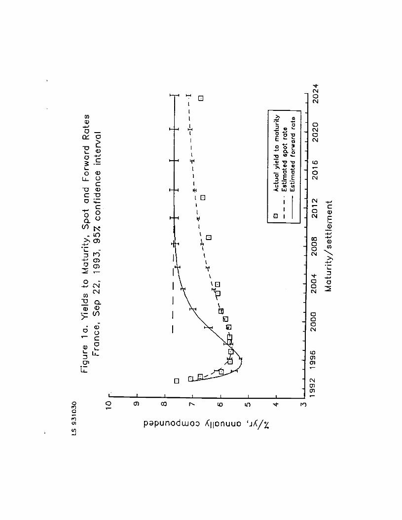
theory.Figure Ia shows actual market bond yields and estimated spot and forward rates

for France, for the trade date September 22, 1993. The squares show quotes of the

overnight rate, Treasury bill yields and government bond yields, annually compoundedand expressed in percent per year, and plotted against the maturity date.1° The dashedcurve shows estimated spot rates plotted against the maturity date. The solid curve shows

estimated instantaneous forward rates plotted against settlement (and maturity, since the

two coincide for instantaneous forward rates). The forward rates approach a constantvalue for long maturities, marked by a horizontal line with long dashes. Error bars on the

spot and forward rate curves denote 95 percent confidence intervals. See Appendix 1 for

details on the estimation.We see that the French spot curve on September 22, 1993, had a U-shape somewhat

similar to the standard shape of average cost curves in microeconomics. Consequentlythe forward rate curve has a shape somewhat similar to the standard shape of marginal

cost curves. The spot and forward rate curves start for zero time to maturity in thesame point, the forward rate curve lies below the spot rate curve while the spot rate is

decreasing in the time to maturity, the forward rate curve cuts the spot rate curve at the

latter's minimum, and the forward rate curve lies above the spot curve when the latter is

increasing. When for long times to maturity the forward rate becomes constant, the spot

rate asymptotically approaches the same constant.Since spot rates and forward rates can be derived from each other, they contain the

same information. Using forward rates instead of spot rates is hence just presentingthe same information in a different way. Using forward rates is an advantage when the

emphasis is on expected future time paths of relevant variables rather than expected future

time averages àf these variables.

Next I shall discuss how forward rates can help to infer market expectations about

'°The rates in the graphs are annually compounded, since that is the standard Way to express interestrates, even though the equations and computations are easiest with continuously compounded rates.

9

future interest rates, inflation rates and future currency depredation rates.

4. Expected Future Interest Rates

Under subjective certainty (perfect foresight, or point expectations) the forward ratef(t, t', T) for a given settlement date C and maturity date T will equal the expectedfuture spot rate i(t', T) with trade date equal to the forward contract's settlement dateand maturity date the same as the forward contract. Thus, the instantaneous forwardrate will equal the expected future instantaneous spot rate (the future overnight rate).

Why is this? The reason is that a forward contract that involves lending at a futuredate, the settlement date, can be financed at the settlement date by borrowingon the spotmarket at the settlement date. Then the difference between the predetermined forwardrate and the spot rate determined on the settlement date, f(i, C, T) —i(t', T), is the excess(nominal) return on the forward contract. Under subjective certainty that excess returnmust be zero.

Under subjective uncertainty, the excess return on the forwardcontract is uncertain atthe trade date, since the future spot rate is uncertain. Whether the forward rate equalsthe expected future spot rate then simply boils down to whether the expected excessreturn on the forward contract is zero or not. The expected excess return on the forwardcontract is the forward term premium, (t, C,T). Hence, the expected future spot rate isthe forward rate less the forward term premium, -

Ei(1', T) 1(4 t',T) — p(t, t', T). (4.1)

Hence, whether the forward rate indicates the expected futurespot rate is simply a matterof the size and the sign of the forward termpremium.

Older theories of the term premium include the liquidity preference theory, whichimplies a positive holding period term premium (see below), and the preferred habitattheory, according to which the term premium for different settlementsdepend on relativesupply and demand from investors with different horizons. More recent asset pricingtheory (see Shiller (1990) and Svensson (1993b)) explains each premium as dependingupon the covariance of the relevant real excess return with the real return on the marketportfolio (CAPM), real consumption (consumption-based CAPM), or the marginal rateof real consumption (general asset pricing model). From the more recent theories thereseems to be no prior as to the sign and magnitude of the term premium.

10

The discussion of term premia in the literature is complicated by the fact that there are

actually three different (but related) term premia that need to be distinguished (Shiller

(1990)). Aside from the forward term premium there is the holding period term premium

(the expected excess return of holding a long bond a short period over the short interest

rate) and the rollover termpremia (the expected excess return of holding along bond to its

maturity over the return from rolling over a short bond to the long bond's maturity) (see

Appendix 2 for precise definitions). The literature has mostly discussed holding periodterm premia for, say, 10-year bonds held for 1 year. This premium is 9 times the forward

term premium with settlement in 1 year and maturity in 10 years. This is a combination

of settlement and maturity that is hardly relevant for monetary policy; the forward term

premia that are relevant would rather have settlement in 2-4 years, say, and maturity one

year after. There are very few estimates in the literature of forward term premia withthat combination of settlement and maturity."

McCulloch (1975, Table 6) reports average (unconditional) forward term premia for USmonthly Treasury bills and Treasury bonds data for the period 1946-1966. For settlement

in 1-5 years and maturity 1 year later he finds positive but small prernia, 0.03-0.10 percent

per year, not significantly different from zero. For settlement in 10 years and maturity 1

year later the premium is -1.09 percent per year, not significantly different from zero.For the period 1952-1987 I have estimated unconditional forward term premia on a

database presented in McCulloch (1990), for settlement in 1-4 years and maturity 1 year

later.'2 The result is displayed in Table I. The premia are fairly small and negative, be-

tween -0.10 and -0.62 percent per year, not significantly different from zero (the premium

for settlement in 4 years is close to being significant, though).'3

Conventional wisdom says that yield curves often have a positive slope (that is, theyield spread between long and short rates is positive). This is sometimes taken as implying

positive term premia. That implication is not correct, though. Term prernia can be small

or even zero even if the yield spread is positive: Suppose short rates are increasing over

the sample period (this is the case for samples ending with the 1980s). Suppose term

ttcampbell and SMiler (1991) test and reject the expectations hypobtesis for a number of differentcombinations of different maturities and settlement. They do not report estimates of term premia,though. Frachot and Lease (1993) derive term premia in a model of the term structure with stochasticconditional volatility and are able to explain the empirical results of Campbell and Shifler (1991).

"This is the seine dataset that Campbell and Shifler (1991) uses.'3For VS data, for settlement in 2-4 years and maturity 1 year later, Fame and Bliss (1987) cannot

reject the hypothesis that forward rates forecast future interest rates and that forward term premia arezero.

11

premia are zero, so tong rates equal expected average short rates up to the long bondmaturity. If short rates are expected to increase, expected future short rates and hencecurrent long rates are of course higher than current short rates.

To check this, I have estimated the average yield spread between 1-10year maturitiesand the 3-month maturity, on McCulloch's (1990) dataset. The result is reported inTable 2. The average yield spread is positive, between 0.37 and 0.81 percent per year,and significantly different from zero. This is so even though term premia are small andnegative.

The premia reported here are average, unconditional, termpremia. It is, however, theconditional time-varying preinia that are relevant in (4.1). Even if unconditional termpremia are small, it is possible that time-varying term premia can be sometimes large. Iftime-varying premia are forecastable and economically significant, forward rates shouldbe adjusted by the premia in order to infer expected future interest rates. Then thetime-varying premia should be estimated simultaneously with thespot and forward rates.If time-varying term premia are not forecastable, the forward rates should be adjustedwith the unconditional term premia. The estimates ofthese reported here indicate thatthey are rather small, though. However, even if the term premia were large, if they wererelatively stable, shifts over time in unadjusted forward rate curves would still containinformation, even if the level of the curves would be less reliable.

In the rest of the paper I shall assume that the term premia relevant for monetarypolicy are negligible, and that forward rates indicate expected future spot rates.

Treasury bill and government bond yields fluctuatequite a bit from day to day, per-haps depending upon temporary excess demand or supply for different maturities. Con-sequently estimates of spot and forward rates fluctuate quite a bit from day to day. I donot want to assume that these short-mn fluctuations necessarily reflect short-run changesin expected future spot rates. Instead the assumption is that forward rates indicate ex-pected future spot rates when these short-run fluctuations are filtered out. Therefore,throughout one should use for instance moving averages over one or a few weeks, ratherthan estimates for a particular day. For convenience only, the examples in this paper willrefer to estimates for single dates.

Figure lb shows spot rates (dashed curves) and forwardrates (solid curves) on Septem-ber 22, 1993, for France (thick curves) and Britain (thin curves). Consider expectationsof future monetary policy for France, as manifested by the overnight rate. We see thatthe expected overnight rate is expected to be lowered to almost 5 percent per year at the

12

end of 1995. From 1996 onwards the over-night rate is expected to increase to about 7

percent per year by year 2001. For Britain, the overnight rates are expected to increasefrom a bit more than 5 percent per year to reach 8 percent per year in year 2000.

How should such expected increases in the overnight rate be interpreted? Could they

be interpreted as an expected future monetary contraction because of expected futureinflation? Hardly. If the central bank is expected to react to higher inflation with amonetary contraction this would be incorporated into price-setting behavior, in which case

the higher inflation and resulting contraction would not occur, and hence not be expected

to occur. An expected increase in overnight rates might reflect a return to normal short

real rates if these are currently abnormally low. Current French and British short real

rates do not seem to be abnormally low, though.'4 Instead it seems that the expectedincrease in overnight interest rates must be interpreted as an expected accommodation

of the central bank to a situation of higher inflation, higher money growth, and higher

interest rates due to Iowa demand for real money balances. Inflation expectations willbe further discussed in the next section.

Whereas the forward rates indicate the expected time-path of future short interest

rates, the spot rate for a particular maturity indicates the expected average short ratesup to that maturity. The British spot rate of 7 percent per year for maturity in year 2000is hence the average short rate between 1993 and 2000.

What about expected future interest rate differentials across countries? From (4.1)and its foreign analog we get that the expected future interest rate differential between

the domestic and foreign country fulfills

Ei(t', T) — Ei(t', T) f(t, t', T) — f(t, C, T) — [y(i,C, T) — rp(t, C, T), (4.2)

where foreign variables are denoted by an asterisk. The expected future interest ratedifferential equals the difference between the domestic and foreign forward rates less the

difference between the domestic and foreign forward term premia. If the premia are of

the same sign and magnitude they will hence cancel.

Assuming that the premia are either negligible or that they cancel, we can use thedifference between the French and British forward rate curves in Figure lb to infer the

Bank of England (1993a) displays a real forward rate curve (derived from the British index-linkedgifts) that does not indicate an expected rapid increase in short real interest rates. In May 1993 the realforward rate for settlement in 2 years was 3 percent per year. It increases slowly with settlement andreaches 4 percent per year for settlement in about 14 years.

13

expected future interest rate differential between the two countries. The differential is

obviously expected to go from almost minus 2 percentage points to plus 2 percentagepoints in about 4 years.

5. Expected Future Inflation Rates

Let r(t, T) and ir(i, T) denote the real spot interest rate and the inflation rate, respectively,between times i and T, T > i.15 Under subjective certainty the Fisher equation holds.

That is, the future inflation rate ir(t', T) between time C and T that is expected at timei, t c C c T, is equal to the difference between the expected future nominal and real spotrates between times I' and T, 1(2', T) — r(i', T). Under subjective certainty the nominalforward rate equals the expected nominal future spot rate. Furthermore, if there is market

for real bonds, the real forward rate equals the expected real future spot rate. Hence, the

expected future inflation rate equals the difference between the nominal and real forwardrates.

With subjective uncertainty, the expected future inflation rate is no longer necessarily

equal to the difference between expected future nominal and real spot rate. Instead aninflation risk premium O(t, 2', T) enters, so we have

Egr(t', T) Ei(t', T) — Etr(t', T) — 0(1, L', T). (5.1)

The inflation risk premium is the expected real excess return on nominal bonds over real

bonds. According to standard theory it depends on the covariance between thatexcessreturn and the return on the market portfolio (CAPM), consumption (consumption-based

CAPM) or the marginal rate of substitution (general asset-pricing model) (see Svensson

(199Th)). Furthermore, we have seen in (4.1) that the expected nominal futurespot rateequals the nominal forward rate less the (nominal) term premium. Hence, the expectedfuture inflation rate is related to the forward rate as

En(t, i',T) f(i, t',T) — E1r(t', T) — w(t, t', T) — 0(2, i', T). (5.2)

With a market for real bonds, as in Britain, the expected future real spot rate is related

"The inflation rate rQ,T) is defined as r(1,T) = JnIP(!?(I)1, where P(i) is the price level at timeS.

14

to the real forward rate, g(t, t', T), via the real (forward) term premium, '(t, jlT),

Egr(t',T) g(t,t',T) — '(i,t',T). (5.3)

It follows that the expected future inflation rate can be written

Egir(t, 9, T) f(t, 9, T) — g(i,9, T) — [y(t, 9, T) — '(t, 11, T)] — O(t,I', T), (5.4)

the difference between the nominal and real forward rates, less thedifference between thenominal and real term premia, less the inflation risk premium.

If there is a market for real bonds, expression (5.4) can be used. If the nominal and

real term premia are of the same sign and magnitude they will cancel. The inflation risk

premium should be small in an economy with real bonds, since with real bonds in themarket portfolio the correlation between inflation and the return on the market portfolio

should be less. Then expression (5.4) should be a rather reliable measure of expectedfuture inflation rates.'6

Without a market for real bonds, only expression (5.2) can be used. The estimated

expected future inflation rate will be contingent upon an assumed expected future realinterest rate.

As mentioned the inflation risk premium depends on the covariance between the excess

real return on nominal bonds over real bonds and the return on the market portfolio,

consumption or the marginal rate of substitution, depending upon which asset pricingmodel is used. The excess return is simply the negative of the rate of inflation. Theinflation risk premium then depends on the covariance between inflation and the variables

mentioned. Whether the inflation premium is positive or negative depends (in CAPM)on whether inflation is negatively or positively correlated with the return on the market

portfolio. A priori it is not obvious which sign the inflation risk premium will have.Regardless of the sign, the correlation between inflation and the return on the market

portfolio is probably not large, in which case the inflation risk premium is unlikely to be

large.In the rest of the paper I shall assume that the inflation risk premium is negligible.

Assume that the expected future real spot rate for France and Britain will be between

'6Bank of England (1993a,b) reports inflation expectations for Britain by subracting a real impliedforward rate curve from a nominal forward rate curve. The real fbrward rate curve is estimated fromyields on the British index-linked gUts. Woodward (1990) has previously used data on the index-linkedguts to compute the term structure of inflation expectations for Britain.

15

3 and 4 percent from 1996 onwards.'7 Then in Figure lb we conclude that the expected

French inflation rate for 1996 is 1.5-2.5 percent per year, since the forward rate for that

year is about 5.5 percent per year. The expected inflation rate rises somewhat to 3-4percent per year around year 2001. The expected future British inflation rate is 3.5-4.5

percent per year in 1996 and increases further to 4-5 percent per year around year 2001.

The difference between the nominal spot rate for given maturity and an assumed real spot

rate would indicate the expected average inflation rate for that maturity. The differencebetween the nominal forward rate for a given settlement and an assumed future real rate

indicate the expected future inflation rate at the time of the settlement. Hence, theforward rate curve indicate the expected time-path of the inflation rate, whereas the spotrate curve indicates the expected average future inflation.

What about expected future inflation differentials across countries. From (5.2) andits foreign analog follows

Etff(2, t', T) — E1r(t,2', T) 1(2, 2', T) — f(t,2', T) — [Etr(2', T) — E1r(t', T)]—[w(2, t', T) — y(t, il, T)J — [0(2, 2', T) — 0(1, t', T)].

(5.5)The expected inflation rate differential is equal to the difference between the forwardrates, less the difference between the expected real rates, less the difference between the

term premia, less the difference between the inflation risk premia. If expected future real

rates, term premia and inflation risk premia are similar across the countries, the forwardrate difference is a good indicator of the expected future inflation differentials.

In Figure ib, for 1996 and a few years after, the expected inflation for Britain is about

2 percentage points higher than for France.

6. Expected Future Currency Depreciation Rates

Under subjective certainty the expected future depredation rate between time 2'and timeT > 2' of the domestic currency relative to the foreign currency, 8(2', T), must equal the

'TThis is consistent with the real forward rate curve presented in Bank of England (1993a). Notethat tt does not make sense to assume a given expected real except at Least a couple ofyears into thefuture. In the short run there is considerable inertia in the price level and the inflation rate. With someaamphflcation: in the short run the inflation is sticky and the real rate adjusts to the nominalrate; themedium and long rim the real rate is sticky and the nominal rate adjusts to the expected inflation rate.

16

expected future interest rate differential, i(i', T) — i(t',T).18 Under subjective ceitainty

the forward foreign exchange risk premium, eQ, V, T), enters into the relation,

Efi(i',T) Ei(t',T) — Ei(t',T) — C(i,t',T), (6.1)

so the expected future currency depreciation rate equals the expected future interest rateless the forward foreign exchange risk premium.

The forward foreign exchange risk premium is the expected excess nominal return on

domestic currency bonds over foreign currency bonds. It depends on the covariance with

the nominal return on the market portfolio (CAPM) or the nominal mirginal rate of

substitution (general asset-pricing model) (see Svensson 1993c)).Uncovered interest parity is the same thing as zero foreign exchange risk premia.

Uncovered interest rate parity is usually empirically rejected, except for the franc/markexchange rate (see Rose and Svensson (1993), for instance). However, attempts to estimate

the size of foreign exchange risk premia have usually resulted in very small premia (see

Hodrick (1987) and Marston (1993) for surveys).

In the rest of the paper I shall assume that the foreign exchange risk premium is

negligible.From (4.2) follows that the expected currency depreciation rate fulfills

E6(i', T) = f(i, t', T) — f(t,1', T) — (p(t, jI,T) — wit, 1',T)J — (t, i', T), (6.2)

the difference between the forward rates, less the difference between the term premia, less

the foreign exchange risk premium.If the term premia are assumed to cancel, and the foreign exchange risk premium is

assumed to be negligible, the vertical distance between the French and British forward

rate curves show the expected future depreciation rate of the franc relative to the pound.

The vertical distance between the French and British spot curves shows the average rate

of depreciation up to the maturity date.

Figure Ic shows the expected future depredation rate (dashed curve) and expected

"Let eQ) denote the log exchange rate (log of units of domestic currency per unit of foreign currency).Then the domestic currency depreciation rate 6(t, 7') i defined as

L(t,T)5

17

future accumulated log depredation (solid curve) of the franc relative to the pound.'9Hence the dashed curve is the slope of the solid curve. We see that the franc is expectedto depredate initially but appreciate eventually by more than 10 percent in the next 10

years.

7. Comparison of Monetary Policies

This section compares monetary policies in France, Germany, Britain, Sweden and theUnited States with the help of graphs of spot and forward rates as weU as of expected

future exchange rates. Figures 2a, Ii and 3a, 6 show spot and forward rates by countryand by trade date. The six trade dates are September 14 and 21 for 1992 (before and

after Black Wednesday, September 16, 1992); February 5, May 7, August .2 (immediatelyafter the July crisis 1993) and September 22 for 1993. The first five dates are chosen tocoincide with those for which Bank of England's model Inflation Report report Britishforward rates (Bank of England (1993cr, 6)). The British forward rates estimated here

correspond closely to those reported by Bank of England, although they are computedwith different methods.2°

Spot and forward rates have been estimated with the help of selected Treasury billand government bond yields for each trade date, with a method described inAppendix 1.The estimates should really be done with all the reasonably liquid bills and bonds, andwith a fair amount of detailed institutional knowledge of each country's bill and bondmarket. A few different estimation methods should also be tried. The graphs presentedhere should therefore be considered as indicative only.

Graphs of forward rates lend themselves very well to studies of particular events,and the graphs should really be interpreted by researchers with detailed knowledge ofmonetary policy events in each country. Lacking such knowledge for countries other than

Sweden, I will here only present some broad impressions, and instead invite specialists on

'The expected accumulated log depreciation is given by

= Egt(t,T)(T— t), T> t.Under the assumption of a negligible foreign exchange risk premium (uncovered interest parity) it fulfills

Eie(T)—e(t) = (i(t,T)—i' (1, T))(T—t).

20Bank of England computes forward rates from a par yield curve, the estimation of which is describedin Bank of England (1990) and Mastronikola (1991).

18

each country for more detailed interpretation.

Consider Figure Sa which shows instantaneous forward rates by country. Central banks

control interest rates at the shortest maturities (overnight or weekly rates, say). Central

banks therefore control the left end-point of each forward rate curve (the shortest forward

rate coincides with the shortest spot rate). The rest of the curves is determined by the

market, and can be interpreted as the market's expectations of future short rates, henceof future monetary policy as it is manifested in the short rates central banks set. Theexcess of the forward rates over a given expected future real spot rate can be interpreted

as the expected future inflation, and differences between countries' forward rates can

be interpreted as expected future currency depreciation rates1 all under the maintainedassumption that the relevant prernia are either negligible or cancel. Even if the premia axe

not negligible or do not cancel, as long as they are stable over time, shifts in the curvesconvey information even if levels cannot be interpreted.

However, let me repeat that I do not want to assume that day-to-day fluctuationsin estimated forward rates should be interpreted in this way, instead the interpretationconcerns averages over one or a few weeks, say. The estimated spot and forward rates to

be discussed are nevertheless for simplicity from six single dates only, which is another

reason why only broad impressions rather than a detailed interpretation is presented.

Figure 3a shows that forward rate curves in general have shifted down during the last

year. For the United States longer forward rates have fallen more than shorter, whereasthe opposite is the case for the other countries. The British experience is interesting (it

is also discussed in Bank of England's Inflation Report). The lowering of short rates after

Black Wednesday was followed by a considerable increase (several percentage points) in

long forward rates. Only recently have long forward rates come down to where they were

immediately before Black Wednesday. One interpretation is that monetary expansionafter Black Wednesday, with limited credibility due to Britain's inflation history and lack

of independence of Bank of England, led to a considerable increase in long run inflation

expectations. For France lower short rates have not been followed by increases in the

long forward rates. Only recently have the long forward rates come down somewhat. For

Sweden the lowering of short rates have, as for Britain, been followed by increases in long

forward rates, and only during the last summer have they come down to where they were

immediately before Black Wednesday.

A comparison with Figure Ea for Britain and Sweden shows that the spot rates givea different interpretation than the forward rates. The long spot rates had come down

19

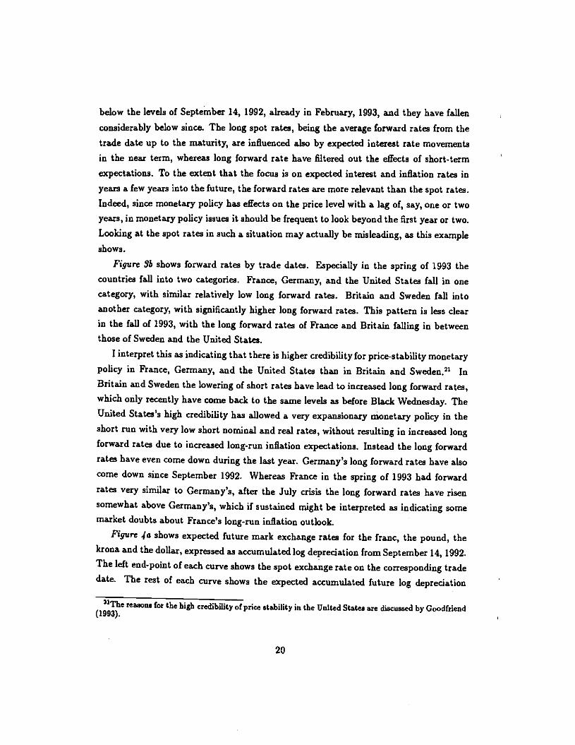
below the levels of September 14, 1992, already in February, 1993, and they have fallen

considerably below since. The long spot rates, being the average forward rates from thetrade date up to the maturity, are influenced also by expected interest rate movements

in the near term, whereas long forward rate have filtered out the effects of short-termexpectations. To the extent that the focus is on expected interest and inflation rates in

years a few years into the future, the forward rates are more relevant than the spot rates.

Indeed, since monetary policy has effects on the price level with a lag of, say, one or two

years, in monetary policy issues it should be frequent to look beyond the first year or two.

Looking at the spot rates in such a situation may actually be misleading, as this exampleshows.

Figure Sb shows forward rates by trade dates. Especially in the spring of 1993 thecountries fall into two categories. France, Germany, and the United States fall in onecategory, with similar relatively low long forward rates. Britain and Sweden fall intoanother category, with significantly higher long forward rates. This pattern is less clearin the fall of 1993, with the long forward rates of France and Britain falling in betweenthose of Sweden and the United States.

I interpret this as indicating that there is higher credibility for price-stability monetary

policy in France, Germany, and the United States than in Britain and Sweden.2' InBritain and Sweden the lowering of short rates have lead to increased long forward rates,

which only recently have come back to the same levels as before Black Wednesday. The

United States's high credibility has allowed a very expansionary monetary policy in theshort run with very low short nominal and real rates, without resulting in increased long

forward rates due to increased long-run inflation expectations. Instead the long forward

rates have even come down during the last year. Germany's long forward rates have also

come down since September 1992. Whereas France in the spring of 1993 had forward

rates very similar to Germany's, after the July crisis the long forward rates have risensomewhat above Germany's, which if sustained might be interpreted as indicating somemarket doubts about France's long-run inflation outlook.

Figure 4a shows expected future mark exchange rates for the franc, the pound, thekrona and the dollar, expressed as accumulated log depreciation fromSeptember 14, 1992.The left end-point of each curve shows the spot exchange rateon the corresponding tradedate. The rest of each curve shows the expected accumulated future log depreciation

(1993).reasons for the high crethbility ofprice stability in the United States are discussed by Goodiriend

20

calculated from the differences between forward rates in Figure 3b. Therefore Figure

4a simply shows the exchange rate expectations that are consistent with the forwardinterest rates and the spot exchange rate on each trade date. The franc had in September

1993 depreciated a few percent relative to the mark, but there were no expectations of

further depredation. The pound had in September 1993 depreciated quite a bit, someappreciation was expected in the short term, and in the long run further depreciation is

expected. For the krona, it appears that during the September 1992 crises, the expecteddevaluation was about 10 percent (see the kink at 10 percent for the curves of September

14 and 21 in 1992). After the krona was floated in November 1992 it has depreciated

rapidly, more rapidly than expected, and in September 1993 further depreciation wasexpected. The dollar has fluctuated relative to the mark quite a bit, but there are noexpectations of substantial future depreciation or appreciation.

8. Conclusion

In the new situation with flexible exchange rates, monetary policy in Europe will haveto rely more on indicators than previously under fixed rates, especially since it will mostlikely be difficult, at least for some time, to find appropriate and reliable intermediatetargets for monetary policy. Several different indicators will have to be used. One of the

potential indicators, the (implied) forward interest rate curve, can be used to indicatemarket expectations of the time-paths of future short interest rates, monetary policy,inflation rates and currency depredation rates.

The forward rate curve contains the same information as the spot rate curve, but itpresents the information in a way that makes it easier to interpret for monetary policy pur-

poses. Thus the forward rate curve separates market expectations for the short, medium

and long term more easily than the spot rate curve. Since monetary policy measures

have effects with "long and variable lags," looking beyond the short term is important

in monetary policy. Using long spot rates or long bond yields instead of long forwardrates can then give misleading impressions, since long spot rates and long bond yieldsinclude expectations of interest rate movements in the short term. In long forward rates

expectations of interest rate movements in the short term have been filtered out:

Monetary policy in France, Germany, Great Britain, Sweden and the United Stateshas been interpreted with the help of forward rates. The British and Swedish experience

is similar in that long forward rates increased considerably after the pound and the krona

were floated, and the long forward rates have come down to pre-September 1992 levels

21

only recently. In contrast, monetary expansion and very low short-term interest ratesin the United States has been followed by a fall in long forward rates. There is someindication of an increase in French long forward rates after the widening of ERM bands in

August 1993. These developments have been be interpreted in terms of movements in long

run inflation expectations. The developments and the interpretation in terms of inflation

expectations are consistent with the idea that long-run credibility for a price-stabilitypolicy increases the scope for monetary policy to stabilize output and employment in the

short run.

The paper has highlighted the role of term, inflation and foreign exchange risk premia

in using forward rates as indicators of future interest rates, inflation rates and currency

depredation rates. The maintained assumption in the analysis of monetary policy in thefive countries considered is that the relevant premia either cancel or are negligible. This

maintained assumption has some empirical support. Estimates of average forward premia

for settlement in a few years and maturity one year later indicate that the premia are

small. Also, the conventional wisdom that upward sloping yield curves imply positive

term prernia is not correct, since the upward sloping yield curve may be explained byexpectations of rising short rates over the sample. However, it is actually conditional time-

varying premia, rather than unconditional average premia that are relevant. More research

on and estimation of unconditional time-varying forward premia with these combinations

of settlement and maturity is called for. The literature has usually considered other term

premia, the holding period and rollover term premia, and other combinations of settlement

and maturity. The literature has also frequently focused on testing the expectationshypothesis (the hypothesis of zero risk premia) rather than on actually estimating thesize of the premia in order to judge whether the premia are economically as well as

statistically significant.

If unconditional time-varying premia are non-negligible, that does not mean that for-

ward rates cannot be used as indicators, only that the premia should be estimated simul-

taneously with the forward rates and then used to adjust the forward rates.

A. Estimation of Spot and Forward Interest Rates

The estimation of spot and forward rates follows McCulloch (1971, 1975) in fitting for

each trade date a discount function (the price of a zero-coupon bond as a function of the

time to maturity) to bill and bond price data, but it uses the functional form of Nelson

22

and Siegel (1987) instead of McCulloch's cubic spline.22

Nelson and Siegel (1987) assume that the instantaneous forward rate is the solutionto a second-order differential equation with two equal roots. Hence it can be written

f(m; /9,r) = o + p1 exp (—) + fi2 exp (—2!), (A.1)

where m � 0 is the time to maturity in years, and where Pa, th, /92 and r are theparameters. The spot rate can be derived by integrating the forward rate according to

(3.5). It is given by

i(m;fl,r)=po+(flt+$)l ex;( ;)—$2exp(_). (A.2)

Let i(0;$,r), f(0;/I,r), i(oo;$,r) and f(co;fi,r) denote the limits of the spot andforward rates when the time to maturity goes to zero and infinity, respectively. The spot

and forward rates have the properties

i(oo;fl,r) = f(oo;fl,r) = Po and (A.3)

i(O; /9, r) = 1(0; /9, r) = Pc + fly. (A.4)

Furthermore, suppose there is a maximum or a minimum for the forward rate, that is,there is an fit � 0 such that the derivative fm(th; /9,r) = 0, with I = f(th; /9, 'r). Then,

!=th+thexP(_1) and (A.5)

(A.6)

It follows that the parameters Pa, fit, /92 and r can be computed recursively by f(oo),1(0), I and fit, which facilitates their interpretation and the choice of starting values inthe estimation procedure.

The discount function is then given by

d(rn; /9, r) = exp[—i(m; /9, i-)mJ. (A.?)

22See Dahlquist and Svensson (1993) for a comparision of estimates of spot and forward rates withthe simple functional form of Nelson and Siegel (1987) and the complex functional form of Longstaff andSchwartz (1992).

23

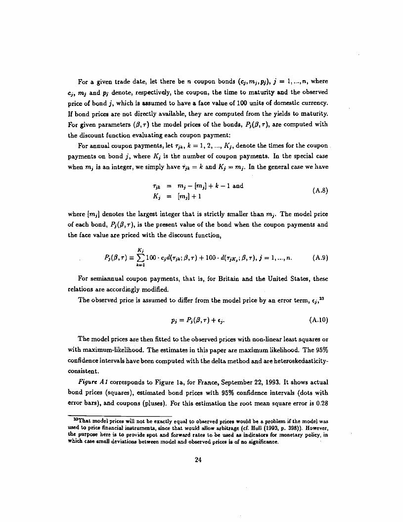
For a given trade date, let there be it coupon bonds (ç,, rn,,p1), j = 1, ..., n, where

c1, rn1 and p denote, respectively, the coupon, the time to maturity and the observed

price of bond j, which is assumed to have a face value of 100 units of domestic currency.

If bond prices are not directly available, they are computed from the yields to maturity.

For given parameters (fi, r). the model prices of the bonds, P,(/3, r), axe computed with

the discount function evaluating each coupon payment:

For annual coupon payments, let rik, k = 1,2,..., K5, denote the times for the coupon

payments on bond j, where K, is the number of coupon payments. In the special case

when rn5 is an integer, we simply have tjk = k and K1 = rn;. In the general case we have

= rna—Lms]+k—1 and(AS)K5 = [rn5]+1

where [m1J denotes the largest integer that is strictly smaller than rn. The model priceof each bond, P;($,r), is the present value of the bond when the coupon payments andthe face value are priced with the discount function,

K,

Pj($,r)E100.cjd(r;k;f3,r)+l0O.d(TKI;/3,r),j=1,...,n. (A.9)k=1

For semiannual coupon payments, that is, for Britain and the United States, theserelations are accordingly modified.

The observed price is assumed to differ from the model price by an error term, cj,

= Pj($,r) + c,. (A.1O)

The model prices are then fitted to the observed prices with non-linear least squares or

with maximum-likelihood. The estimates in this paper are maximum likelihood. The 95%

confidence intervals have been computed with the delta method and are heteroskedasticity-

consistent.

Figure Al corresponds to Figure la, for France, September 22, 1993. It shows actualbond prices (squares), estimated bond prices with 95% confidence intervals (dots witherror bars), and coupons (pluses). For this estimation the root mean square error is 0.28

"That model prices will not be exactly equal to observed prices would be a problem if the model wasused to price financial instruments, since that would allow arbitrage (cf. Hull (1993, p. 398)). However,the purpose here is to provide spot and forward rates to be used as indicators for monetary policy, inwhich case small deviations between model and observedprices is of no significance.

24

percent of the bonds's principal value. The maximum error is 0.68 percent of the face value

of the 19-year bond maturing in year 2012. The root mean square error of yield errorsis 0.13 percentage points. The parameters are fib = 0.0746, fl = —00060, th = —0.0571

and r = 2.210. For long maturities the spot and forward rates hence approach the level

7.46 percent per year continuously compounded, which corresponds to 7.75 percent per

year annually compounded.The estimates of the spot and forward rates in this paper has been done with the

restriction that the estimated spot rate and forward rate for zero maturity and settlement

should equal the quoted overnight rate (in practice, that fib and fi' should sum to thequoted overnight rate). In some cases that has lead to a poor fit of the Treasury bill rates

with maturity 3, 6 or 12 months. Then the zero-maturity spot and forward rate has beenadjusted to give a better fit to the Treasury bill rates. In these cases the left end-points of

the spot and forward rate curves of course differ from the quoted overnight rate. Figure

la is one such case. There the zero-maturity spot and forward rate has been set to is

7.1 percent per year annually compounded, which differ from the quoted overnight rate,about 7.5 percent per year annually compounded. This procedure has been followed since

I have trusted the Treasury bill data more than the overnight rate data.

It is desirable that the estimated spot rates should fit the Treasury bill rates well sincethe latter are actual spot rates. There is no reason the estimated spot rates should equal

the coupon bond yields, since the yields depend on the coupons. Therefore, the fact that

the spot rates in Figure la deviate from the bond yields for long maturities does notindicate a bad fit.

Minimizing the squared deviations from Treasury bill and bond prices gives less weight

to short-maturity yields, since prices are insensitive to yields for short maturities. Unre-

stricted estimates can then give fairly large deviations for short yields. That is the reason

why I have imposed the restriction on estimated zero-maturity spot and forward rates.

Alternatively, the price deviations can be weighted somewhat in favor of short maturities.

Minimizing deviations from yields is of course an implicit strong weighting of short ma-

turities. In general, the weighting should be motivated by the purpose of the estimation,

especially in which maturity range most precision is desired.

Convergence was fast with reasonable starting values, especially when the parameters

fi' and $2 were scaled by 100.

See Dahlquist and Svensson (1993) for further discussion of these and related issues.

25

B. Three Different Term Premia

As discussed in Shiller (1990) there are threekinds of term premia that have been discussed

in the literature. The forward term premium ç(t, 1', T) is defined as

p(t, 2', T) f(t, I',T) — Ei(t', T). (13.1)

The holding period term premium rph(t, 1', T) is defined as

'P4@, t', T) E1h(t, 2', T) — 1(2, 9), (8.2)

where the holding period return h(t, 1', T) is the rate of return from holding a bondmaturing at time T from time 2 to time t', which gives

h(L, 2', T)1(2,T)(T — t)—i(t', T)(T — 2')

(B3)

The rollover term premium çt',(i,T, m) is defined as

ço,(t,T,m) = i(1,T) — (2 + U — 11)m,t +jrn), (13.4)

where m = and n is an integer, the number of times a bond of maturity m is rolledover.

The following relations hold between these term premia:

(ph(t, 9, T)w(t t',7')(T — 2')

(13.5)

w@,t', T) 1y(t, t + (j — 1)m,i + im). (3.6)

26

Table 1. Forward Term Premium (1-year rates, %/yr)

Settlement Premium Std Err1 yr -0.10 0.22

2 yrs -0.24 0.36

3 yrs -0.44 0.36

4 yrs -0.62 0.34

Table 2. Yield spread (over 3-month yields, %/yr)

Maturity Spread Std Err1 yr 0.37 0.05

2 yrs 0.49 0.10

3 yrs 0.57 0.13

4 yrs 0.63 0.13

5 yrs 0.68 0.13

10 yrs 0.81 0.12

27

References

[1 Alesina, Alberto, and Lawrence H. Summers (1993), "Central Rank Independenceand Macroeconomic Performance: Some Comparative Evidence," Journal of Money,

Credit, and Banking 25, 151-162.

12] Bank of England (1990), "A New Yield Curve Model," Bank of England Quarterly

Bulletin, February 1990, 84-85.

[1 Bank of England (1993a), Inflation Report, May 1993.

[4) Bank of England (1993b), Inflation Report, August 1993.

[5) Bank for International Settlements (1993), 63rd Annual Report, Basle.

[6] Batten, Dallas S., Michael P. Blackwell, In-Su Kim, Simon E. Nocera and Yusuru

Ozeki (1990), "The Conduct of Monetary Policy in the Major Industrial Countries:

Instruments and Operating Procedures," IMF Occasional Paper No. 70.

(7] Bernanke, Ben, and Frederic Mishkin (1992). "Central Bank Behavior and the Strat-

egy of Monetary Policy: Observations from Six Industrialized Countries." NBERMacroeconomics Annual 1992.

(8] Campbell, John Y., and Robert J. Shiller (1991), "Yield Spreads and Interest Rate

Movements: A Bird's Eye View," Review of Economic Studies 58, 495-514.

[9] Dahlquist, Magnus, and Lan E. 0. Svensson (1993), "Estimation of the Term Struc-

ture of Interest Rates with Simple and Complex Functional Forms: Nelson & Siegel

vs. Longstaff & Schwartz," Working Paper.

[10) Fama, Eugene F., and Robert R. Bliss (1987), "The Information in Long-MaturityForward Rates," American Economic Review 77, 608-692.

(11) Frachot, Antoine, and Jean-Philippe Lesne (1993), "Expectations Hypotheses and

Stochastic Volatilities," Working Paper, Banque de France.

[12] Freedman, Charles (1993), "Formal Targets for Inflation Reduction: The Canadian

Experience," Working Paper, Bank of Canada.

28

[13] Friedman, Benjamin M. (1990), "Targets and Instruments of Monetary Policy,"Chapt. 22 in Friedman, Benjamin M. and Frank H. Hahn (eds), Handbookof Mont-tary Economics, Volume II, North-Holland, Amsterdam.

(14] Goodfriend, Marvin (1993), "Interest Rate Policy and the Inflation Scare Problem:1979-1992," in Marvin Goodfriend and David H. Small, eds, Operating Proceduresand the Conduct of Monetary Policy. ConferenceProceedings, Federal Reserve Board,Washington, D.C.

[15] Hodrick, Robert J., (1987), The Empirical Evidence on theEfficiency of For-ward andFutures Foreign Exchange Markets, Harwood Academic Publishers, London.

[16] Hörngren, Lars, and Hans Lindberg (1993), "The Struggle to Turn the SwedishKronainto a Hard Currency," Working Paper No. 8, Sveriges Riksbank.

[17] Hull, John C. (1993), Options, Futures, and Other DerivateSecurities, Second edi.tion, Prentice-Han, London.

[18] Marston, Richard C. (1993), "Nominal Interest Differentials," manuscript chapter.

1191 Mastronikola, Katerina (1991), "Yield Curves for Gilt-Edged Stocks: ANew Model,"Bank of England Discussion Paper, Technical Series, No. 49.

1201 McCallum, Bennett T. (1990), "Targets, Indicators and Instruments of MonetaryPolicy," IMF Working Paper WP/90/41.

1211 McCulloc, J. Huston (1971), "Measuring the Term Structure of Interest Rates,"Journal of Business 44, 19-31.

1221 McCulloch, J. Huston (1975), "An Estimate of the Liquidity Premium," Journal ofPolitical Economy 83, 62-63.

(23] McCuiloch, J. Huston (1990), "US Term Structure Data, 1946-1987," Appendix Bin Shiller (1990).

(24J Nelson Charles R., and Andrew F. Siegel (1987), "ParsimoniousModeling of YieldCurves," Journal of Business 60, 473.489.

(25) Rogoff, Kenneth (1985), "The Optimal Degreee of Commitment to an IntermediateMonetary Target," Quarterly Journal of Economics 100, 1169-1189.

29

[261 Rose and Svensson (1993), "Expected and Predicted Realignments: The FF/DM

Exchange Rate during the EMS, 1979-1993," Working Paper.

[27] Shiller, Robert J. (1990), "The Term Structure of Interest Rates," Chapt. 13 inFriedman, Ben M., and Frank H. Hahn (eds), Handbook of Monetary Economics,Volume I, North-Holland, Amsterdam.

[28] Svensson, Lars E.O. (1992), "Targets and Indicators with a Flexible Exchange Rate,"

Monetary Policy with a Floating Exchange Rate, Sveriges Riksbank, December 1992,15-24.

129] Svensson, Lars E.O. (i993a), "The Forward Interest Rate Curve - An Indicator ofMarket Expectations of Future Interest Rates, Inflation and Exchange Rates" (inSwedish), Ekonomisk Debatt 21-3, 219-234.

[301 Svensson, Lars E.O. (1993b), "Term, Inflation and Foreign Exchange Risk Premia:A Unified Treatment," Seminar Paper No. 548, Institute for International EconomicStudies.

[311 Svensson, Lars E.O. (1994), "Fixed Exchange Rates as a Means to Price Stability:What Have We Learned?" European Economic Review, forthcoming.

[32) Sveriges Riksbank (1993), Monetary Policy Indicators, June 1993.

[33] Woodward, C. Thomas (1990), "The Real Thing: A Dynamic Profile of the TermStructure of Real Interest Rates and Inflation Expectations in the United Kingdom,

1982.89," Journal of Business 63, 373-398.

30

LS 9

3103

0

0 a)

•0

C J 0 a F 0 0 >' 0 C

C

0

10

Fig

ure

1 a.

Y

ield

s to

kiu

turit

y,

Fra

nce,

S

ep 22

, S

pot

and

For

war

d R

ates

in

terv

al

1993

, 95

Z c

onfid

ence

0

9 8 7

6 5 4

3

ci

1992 1996

20D0

I I

I I

i I

I

0 A

ctua

l yie

ld t

o m

atur

ity

— —

—

E

etIr

note

d sp

ot r

ate

Est

imat

ed f

orw

ard

rate

2004

2008

2012

Mat

urity

/set

tlem

ent

I I

2016

2020

2024

-c

4)

-o

C J 0 a E

C

C) >

0 C c a

10

Fig

ure

lb.

Spo

t an

d F

orw

ard

Rat

es,

Fra

nce

arid

C

reat

Brit

ain

Sep

22,

19

93

9

S 7 6

5

4

3

9_

I I

I I

— —

—,

Fra

nce.

ep

ot

rate

F

ranc

e. fo

rwar

d ra

te

— —

—.

Gre

at

Brlt

cfn,

sp

ot r

ate

Gre

at B

ritai

n. f

orw

ard

rate

I

I I

I

1994 1995 1996 1997 1998 1999 2000 2001 2002 2003 2004

Maturity/settlement

N

0

—4

—6

—8

—10

Fut

ure

Dep

reci

a D

epre

ciat

ion,

F

RF

/GB

P.

— —

—

Exp

ecte

d E

xpec

ted

futu

re d

epre

ciat

ion

futu

re a

ccum

ulat

ed ra

te,

7./y

r lo

g de

prec

iatio

n. 2

—

12

I

1994

1995 1996 1997 1998 1999 2000 2001 2002 2003 2004

Fig

ure

ic.

Exp

ecte

d

2

tion

Rat

e an

d S

ep

22,

1993

—2

Acc

u m

ulat

ed

Figure 2a. Spot Rates by Counb-yFrance Germany

—Sep 14, 199212 Sep 21, 1992 12

—'Vet, 5.1993¼ '—'•Moy 7, 199310 .'. —Auv 2. 1993 10

8 8

5

1994 lSfl $998 2000 2002 2004 ?992 1994 1996 1998 2000 2002 2004Maturity

Great Britain Sweden

1994 1996 1998 2000 2002 2004 12992 1994 )996 1998 2000 2002 2004

United States12

10

1492 1994 1996 1996 2Q00 2002 2004

12VVCCa.£

C.6CC

Figure 2b. Spot Rates by Trade Date

12

10

a

6

4

(992 1994

Feb 5, 199312

10

a

6

4

1996 i990 2000 2002 2004 92

May 7, 1993

1994 1590 1990 2000 2002 2004

Aug 2. 1993

1994 1996 1990 2000 2002 2004

Sep 14, 1992

—— Swsd.n— United State.

Sep 21. 199212

10

92 1994 1996 1998 2000 2002 20041992 1994 1996 19982000 2002 2034Ucturity

12

10

e

6

4

12

Sep 22, 1993

a

6

4

h92 1994 1996 1998 2000 2002 2004

SVC3C

12

10

8

6

4

92 1994 1996 i998 2000 2002 Z(Y4

12

10

United States

12

10

8

8

4

?992 1994 199$ 1998 2000 2002 2004

a

6

4

"992 1994 1996 1996 2000 2002 2004

12

Figure 3o. Forward Rates by CountryFrance Germany

12

10

a

6

4

Settlsrnsnt1994 1998 1998 2000 2002 2004

Great Britain Sweden

— Franc.—. Ganiany

Gr.at BritainSwudsn

—United Stales

i4az 1994 1696 1998 2000 2302 2304

6

Sotti. ens nt

Feb 5, 1993 May 7, 199312

10

a

4

(9Z 1994 1996 1998 2000 2002 2004 i992 1994 1996 1998 2000 2002 2004

Aug 2, 1993 Sep 22, 199312

10

&92 1994 1996 1996 2000 2002 2004 f992 1994 1996 1998 2000 2002 2004

Figure 3b. Forward

Sep 14, 1992

12

Ig 100

Pates by Trade Date

Sep 21, 1992

12

10

8

8

4

19e2 1994 1996 1998 2000 2002 2004

12

10

8

4

8

12

10

6

4 I/

6

6

4

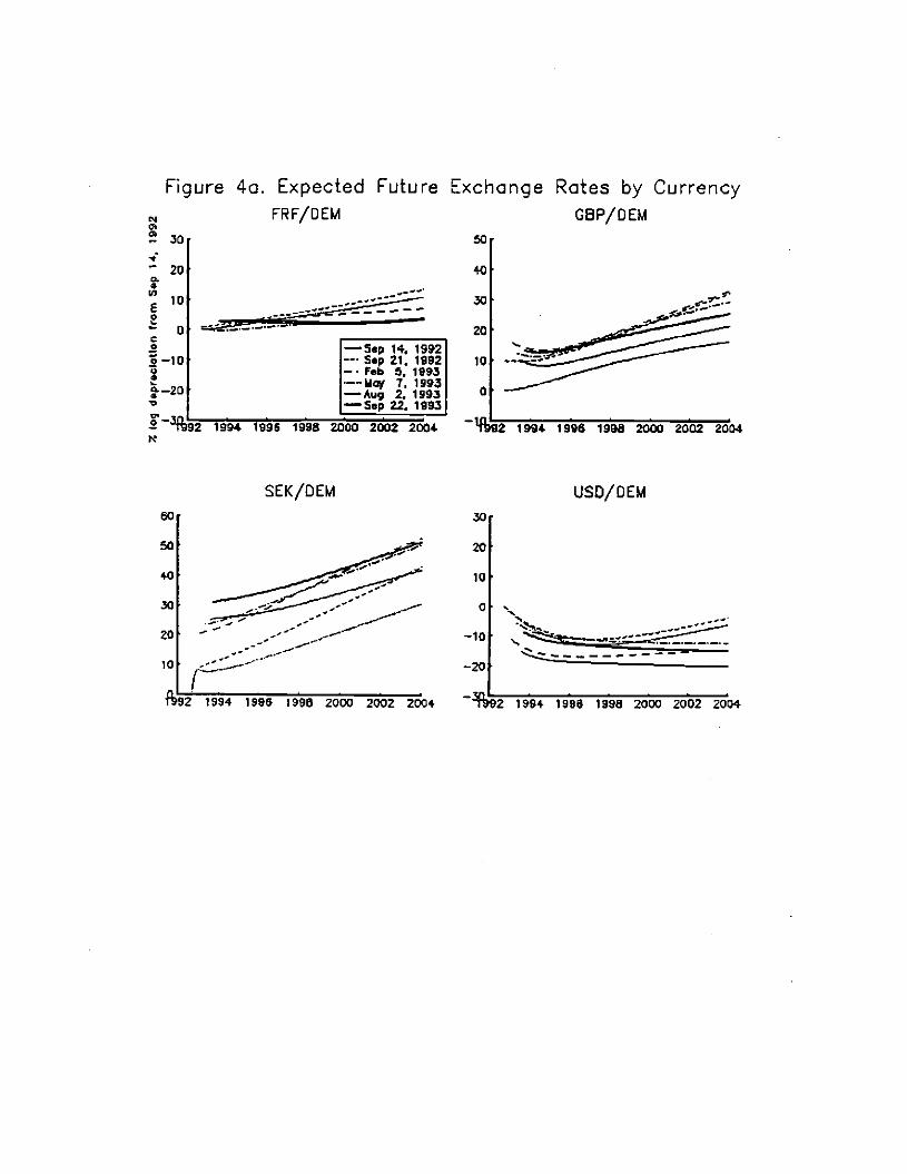
Figure 4a. Expected Future Exchange Rates by Currency

SEK/DEM IJSD/DEM60 .30

50

40

-20

tbs2 1994 1996 1996 2000 2002 2004 tb92 1984 1986 1998 2000 2002 2004

FR Ff0 EM GBP/ OEM

50

40

Na30

200.

10

0 '—CC

o—10

—200

1994 1996 1998 2000 2002 2004

20

—'—Sep 14. 1992Sep 21, 1992

—. Feb 5, 1993—-Uay 7, 1993—Aug 2. 1993

Sep 22. 1993

10

0

'Th92 1994 1996 1998 2000 2002 2004

30

20

10

20

10

0

Figure 4b. Expected Future Exchange Rates by Trade DateN Sep 14, 1992 Sep 21, 1992a

60 60— FRF/tiflA—-GW/DEM

1994 1996 1998 2000 2002 2004 Th19Z 1994 1996 1998 2000 2002 2004

Feb 5, 1993 May 7, 199360 60

30-

o

%92 1994 1995 1996 2000 2002 2004 1994 19 1998 2000 2002 2004

Aug 2, 1993 Sep 22, 199360 60

.30

1994 1996 1998 2000 2002 2004 %92 1994 1998 1998 2000 2002 2004

LS 9

3103

0 A

ctua

l an

d E

stim

ated

B

ond

Sep

22

. 19

93.

95Z

con

fiden

ce

100

-

go -

Wf+

E

l El

I I

- _I

__i_

I

I I

I I

Mat

urity

2020

Fig

ure

Al.

130

-

120

-

N

110

-

w

Pric

es,

Cou

pons

. F

ranc

e in

terv

al

di +

a

9 +

+

+

+

Q

Act

ual

bond

-pric

e •

Est

imat

ed b

ond

pric

e +

cou

pon

+

100

1992

19

96

2000

20

04

2008

20

12

2016

20

24