NBER WORKING PAPER SERIES - Dirk Niepelt
43
NBER WORKING PAPER SERIES SOVEREIGN BOND PRICES, HAIRCUTS AND MATURITY Tamon Asonuma Dirk Niepelt Romain Rancière Working Paper 23864 http://www.nber.org/papers/w23864 NATIONAL BUREAU OF ECONOMIC RESEARCH 1050 Massachusetts Avenue Cambridge, MA 02138 September 2017 The authors are grateful to Christoph Trebesch for kindly providing the data. The authors thank Fernando Broner, Luis Catao, Marcos Chamon, Satyajit Chatterjee, Xavier Debrun, Raphael Espinoza, Raquel Fernández, Atish Rex Ghosh, Anastasia Guscina, Juan Carlos Hatchondo, Olivier Jeanne, Luc Laeven, Alberto Martin, Leonardo Martinez, Michael G. Papaioannou, Fabrizio Perri, Guido Sandleris, Damiano Sandri, Sergio Schmukler, Christoph Trebesch, Adrien Verdelhan, Pablo Winant, Mark Wright, Jeromin Zettelmeyer, and participants at 2015 Barcelona GSE Summer Forum (International Capital Flows), IMF ICD, IMF RES, 2016 North American Winter Meeting of the Econometric Society (San Francisco), UC Santa Cruz, and Univ. Osaka for comments and suggestions. The views expressed in this paper are those of the authors and need not reflect the views or the policy of the International Monetary Fund or the National Bureau of Economic Research. This Paper was also published as IMF Working Paper 17/119. At least one co-author has disclosed a financial relationship of potential relevance for this research. Further information is available online at http://www.nber.org/papers/w23864.ack NBER working papers are circulated for discussion and comment purposes. They have not been peer-reviewed or been subject to the review by the NBER Board of Directors that accompanies official NBER publications. © 2017 by Tamon Asonuma, Dirk Niepelt, and Romain Rancière. All rights reserved. Short sections of text, not to exceed two paragraphs, may be quoted without explicit permission provided that full credit, including © notice, is given to the source.
Transcript of NBER WORKING PAPER SERIES - Dirk Niepelt

NBER WORKING PAPER SERIES
SOVEREIGN BOND PRICES, HAIRCUTS AND MATURITY
Tamon AsonumaDirk Niepelt
Romain Rancière
Working Paper 23864http://www.nber.org/papers/w23864
NATIONAL BUREAU OF ECONOMIC RESEARCH1050 Massachusetts Avenue
Cambridge, MA 02138September 2017
The authors are grateful to Christoph Trebesch for kindly providing the data. The authors thank Fernando Broner, Luis Catao, Marcos Chamon, Satyajit Chatterjee, Xavier Debrun, Raphael Espinoza, Raquel Fernández, Atish Rex Ghosh, Anastasia Guscina, Juan Carlos Hatchondo, Olivier Jeanne, Luc Laeven, Alberto Martin, Leonardo Martinez, Michael G. Papaioannou, Fabrizio Perri, Guido Sandleris, Damiano Sandri, Sergio Schmukler, Christoph Trebesch, Adrien Verdelhan, Pablo Winant, Mark Wright, Jeromin Zettelmeyer, and participants at 2015 Barcelona GSE Summer Forum (International Capital Flows), IMF ICD, IMF RES, 2016 North American Winter Meeting of the Econometric Society (San Francisco), UC Santa Cruz, and Univ. Osaka for comments and suggestions. The views expressed in this paper are those of the authors and need not reflect the views or the policy of the International Monetary Fund or the National Bureau of Economic Research. This Paper was also published as IMF Working Paper 17/119.
At least one co-author has disclosed a financial relationship of potential relevance for this research. Further information is available online at http://www.nber.org/papers/w23864.ack
NBER working papers are circulated for discussion and comment purposes. They have not been peer-reviewed or been subject to the review by the NBER Board of Directors that accompanies official NBER publications.
© 2017 by Tamon Asonuma, Dirk Niepelt, and Romain Rancière. All rights reserved. Short sections of text, not to exceed two paragraphs, may be quoted without explicit permission provided that full credit, including © notice, is given to the source.

Sovereign Bond Prices, Haircuts and MaturityTamon Asonuma, Dirk Niepelt, and Romain RancièreNBER Working Paper No. 23864September 2017JEL No. F34,F41,H63
ABSTRACT
Rejecting a common assumption in the sovereign debt literature, we document that creditor losses ("haircuts") during sovereign restructuring episodes are asymmetric across debt instruments. We code a comprehensive dataset on instrument-specific haircuts for 28 debt restructurings with private creditors in 1999-2015 and find that haircuts on shorter-term debt are larger than those on debt of longer maturity. In a standard asset pricing model, we show that increasing short-run default risk in the run-up to a restructuring episode can explain the stylized fact. The data confirms the predicted relation between perceived default risk, bond prices, and haircuts by maturity.
Tamon AsonumaInternational Monetary Fund700 19th Street N.W.Washington, D.C. [email protected]
Dirk NiepeltStudy Center Gerzensee Neues Schloss 3115 GerzenseeSwitzerland and University of [email protected]
Romain RancièreDepartment of EconomicsUniversity of Southern CaliforniaLos Angeles, CA 90097and [email protected]

1 Introduction
Conventional wisdom among practitioners and academics holds that the treatment of private
creditors in sovereign debt exchanges does not vary by the maturity of instruments they hold (In-
stitute of International Finance 2012; 2015).1 After all, the pari passu clause, which is commonly
included in unsecured cross-border corporate and international sovereign debt contracts, provides
that the debt instruments issued under such contracts will rank equally among themselves and
with all other present or future unsubordinated and unsecured external debt obligations of the
borrower (IMF 2014). In line with this view, the empirical literature on sovereign debt restruc-
turings has documented that creditor losses (“haircuts”) tend to be symmetric across private
debt instruments—with a few exceptional restructuring episodes (Sturzenegger and Zettelmeyer
2006, 2008).
In this paper, we challenge the conventional wisdom. Based on a new, comprehensive dataset
on instrument-specific haircuts in 28 sovereign debt restructuring episodes (18 external and 10
domestic) with private creditors over the period 1999–2015, we document that creditor losses
systematically vary by maturity of debt instrument. Specifically, we show that haircuts on
shorter-term debt tend to be larger.
Our finding is robust. It holds when we measure haircuts according to the standard Sturzeneg-
ger and Zettelmeyer (2006, 2008) measure which is computed based both on a market price and
a hypothetical net present value. It also holds when we measure haircuts alternatively, based
on the price of the “old” instrument before the exchange relative to the price of the “new” in-
strument immediately after the restructuring. Our alternative measure can easily be computed
because it only requires observed market prices. Moreover, it can be computed for windows of
different length before the actual restructuring date.
Our finding also is robust when we control for characteristics of the exchanged bonds or
the restructuring episode. For instance, it holds both in external and domestic restructuring
episodes; it holds when restructurings occur preemptively or post default2; and it holds inde-
pendently of the exchange method that is, whether the exchange involves a single menu of new
instruments or different menus depending on type of restructured bonds.3 Cross-sectional re-
gressions controlling for instrument- and episode-specific effects robustly confirm the stylized
fact.
Digging deeper, we find that the negative relation between the maturity of a bond and the
haircut suffered during a debt exchange reflects the fact that ceteris paribus, short-term bond
prices tend to be higher before an exchange than the prices of longer-term debt. In other words,
in the run-up to a restructuring episode, short-term bond prices tend to converge to long-term
1IMF (2015) documents that the terms of exchange often differ along other dimensions including governinglaw, currency denomination, type of instrument, and residency of debt holder.
2Asonuma and Trebesch (2016) define a restructuring as preemptive when the exchange takes place prior toor without a missed payment, and as post-default otherwise.
3In the restructuring cases where the exchange involves different menus depending on type of restructuredbonds, short-term bond holders are often offered menus which include compensations for estimated creditorlosses, i.e. cash payments (“sweeteners”).
1

bond prices from above.
Building on a standard model of arbitrage-free risk-neutral pricing we motivate the stylized
fact as the natural implication of the term structure of default risk and its time variation. As long
as investors anticipate strictly positive default risk after the maturity date of short-term debt,
the price of the latter exceeds the price of longer-term debt (holding all other characteristics
constant). Prices of short-term bonds therefore exceed prices of longer-term bonds, and when a
restructuring episode ends with all outstanding instruments being exchanged against the same
new instrument (or basket of new instruments) then this implies our main stylized fact: A
higher haircut on short-term bonds, measured either way. Moreover, if in the run-up to a debt
restructuring episode investors perceive increasingly short-term default risk then the prices of
short- and longer-term bonds converge. This implies that the extent to which the possible
haircuts vary by maturity weakens as the restructuring event approaches. Intuitively, successive
bad news in the run-up to the restructuring compress price differentials across maturities and
as a consequence, diminish the ex-post haircut differentials as well.
We then explore empirically the theoretical prediction that prices of short- and longer-term
bonds converge because of increasingly short-term default risk. In panel regressions covering the
period from 6 months before the announcement of a restructuring until the date of exchange
or default, and controlling for restructuring-specific factors we find that the data confirms the
prediction.
Our paper relates to the empirical literature on creditor losses due to restructurings, specif-
ically Eichengreen and Portes (1986, 1989), Lindert and Morton (1989), Sturzenegger and
Zettelmeyer (2006, 2008), Benjamin and Wright (2009), Cruces and Trebesch (2013), Finger
and Mecagni (2007), Bedford et al. (2005), as well as Diaz-Cassou et al. (2008).4 Almost
all studies report the average haircuts for the restructuring.5 Only a few (Sturzenegger and
Zettelmeyer 2006, 2008; and Zettelmeyer et al. 2013) document instrument-specific haircuts,
but only for selected restructuring episodes. In contrast, we report instrument-specific haircuts
for a large sample of restructuring episodes; we document a novel stylized fact concerning the
systematic relationship between haircut and maturity; and we offer an explanation for this fact.
Our paper also contributes to the theoretical literature building on Eaton and Gersovitz’
(1981) classic framework and studying the maturity structure of sovereign debt for instance
Rodrik and Velasco (1999), Jeanne (2009), Broner et al. (2013), Arellano and Ramanarayanan
(2012), Chatterjee and Eyigungor (2012), Fernandez and Martin (2014), Aguiar and Amador
(2013), Hatchondo and Martinez (2009), Hatchondo et al. (2016), and Niepelt (2014). These pa-
pers aim at rationalizing why sovereigns choose a specific portfolio composition, often assuming
that haircuts after default are symmetric across bonds with different maturities. We document
that this assumption is not supported by the data, and we offer an explanation for this new
stylized fact which, as we also show, is consistent with other evidence.
The remainder of the paper is structured as follows. Section 2 explains two measures of
4Cline (1995) and Rieffel (2003) contain further haircut estimates for several episodes.5Applying a similar approach, Hatchondo et al. (2014) measure average capital gains on restructured debt.
2
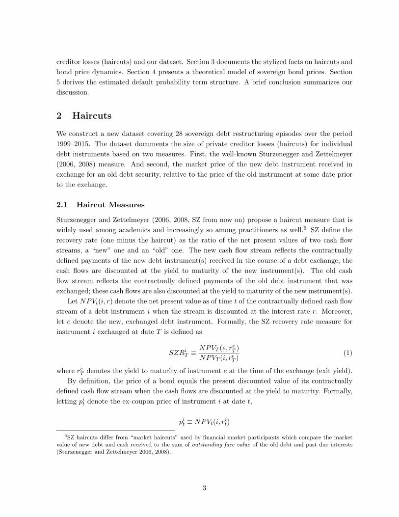
creditor losses (haircuts) and our dataset. Section 3 documents the stylized facts on haircuts and
bond price dynamics. Section 4 presents a theoretical model of sovereign bond prices. Section
5 derives the estimated default probability term structure. A brief conclusion summarizes our
discussion.
2 Haircuts
We construct a new dataset covering 28 sovereign debt restructuring episodes over the period
1999–2015. The dataset documents the size of private creditor losses (haircuts) for individual
debt instruments based on two measures. First, the well-known Sturzenegger and Zettelmeyer
(2006, 2008) measure. And second, the market price of the new debt instrument received in
exchange for an old debt security, relative to the price of the old instrument at some date prior
to the exchange.
2.1 Haircut Measures
Sturzenegger and Zettelmeyer (2006, 2008, SZ from now on) propose a haircut measure that is
widely used among academics and increasingly so among practitioners as well.6 SZ define the
recovery rate (one minus the haircut) as the ratio of the net present values of two cash flow
streams, a “new” one and an “old” one. The new cash flow stream reflects the contractually
defined payments of the new debt instrument(s) received in the course of a debt exchange; the
cash flows are discounted at the yield to maturity of the new instrument(s). The old cash
flow stream reflects the contractually defined payments of the old debt instrument that was
exchanged; these cash flows are also discounted at the yield to maturity of the new instrument(s).
Let NPVt(i, r) denote the net present value as of time t of the contractually defined cash flow
stream of a debt instrument i when the stream is discounted at the interest rate r. Moreover,
let e denote the new, exchanged debt instrument. Formally, the SZ recovery rate measure for
instrument i exchanged at date T is defined as
SZRiT ≡
NPVT (e, reT )
NPVT (i, reT )(1)
where reT denotes the yield to maturity of instrument e at the time of the exchange (exit yield).
By definition, the price of a bond equals the present discounted value of its contractually
defined cash flow stream when the cash flows are discounted at the yield to maturity. Formally,
letting pit denote the ex-coupon price of instrument i at date t,
pit ≡ NPVt(i, rit)
6SZ haircuts differ from “market haircuts” used by financial market participants which compare the marketvalue of new debt and cash received to the sum of outstanding face value of the old debt and past due interests(Sturzenegger and Zettelmeyer 2006, 2008).
3

This implies that the numerator in the SZ recovery rate measure can directly be observed: it is
the price of the new, exchanged debt instrument immediately after the exchange. In contrast,
the denominator of the measure cannot directly be observed and does not have a meaningful
price counterpart: it represents the present discounted value (at the time of the exchange) of
the old debt instrument’s cash-flow stream when discounted at the new debt instrument’s exit
yield. Computing the denominator and thus, the SZ recovery rate requires information about
the cash flow stream of the old instrument as well as the exit yield of the new instrument.
This information requirement poses a problem if one wishes to assess haircuts for many
instruments, as we do. An obvious solution is to replace the net present value in the denominator
of the SZ measure by a different net present value that equals an observed market price. This
is easily achieved by replacing the exit yield in the net present value formula by the yield to
maturity of the old instrument before the exchange. An additional advantage of this approach
is that it opens the way for computing haircut measures that are defined over longer “windows.”
We therefore define the alternative recovery rate measure, “Exchange recovery rate”
Rit,T ≡
NPVT (e, reT )
NPVt(i, rit)(2)
which is, by definition, identical to the ratio of two prices. The numerator on the right-hand
side of equation (2), which is the same as in equation (1), equals the price of the new instrument
immediately after the exchange. The denominator equals the price of the old instrument at
some date prior to the exchange, t ≤ T .
Note that our new measure differs from the SZ measure even for t = T . This difference
reflects the fact that the two measures use different base values to assess the recovery rate.
While SZ use a synthetic value as base value, our measure (computed for t = T ) uses the market
price of the old instrument. In our empirical analysis, we find that quantitatively this difference
is minor,
RiT,T
SZRiT
=NPVT (i, reT )
NPVT (i, rit)≈ 1
While for a single instrument, the dependence of Rit,T on window length T − t may be of limited
interest, the differential dependence for different instruments does provide useful information. In
particular, for two instruments i and j and varying window lengths, T − t, the relative recovery
rates, Rit,T − Rj
t,T , illustrate which instrument’s price converged more quickly to the market
value of the new instruments received in the exchange.
2.2 Data
Our empirical analysis covers 28 episodes with 18 external and 10 domestic sovereign debt
restructurings that involved private creditors, over the period 1999–2015. To date an episode,
we rely on Asonuma and Papaioannou (2016) and Asonuma and Trebesch (2016) for domestic
and external restructuring episodes, respectively. Following these authors, we define the start
4

of an episode as the month in which a default occurs or a distressed restructuring is announced;
and the end of an episode as the month of the final agreement or of the implementation of the
debt exchange.7
We construct a novel comprehensive dataset with information about instrument specific
haircuts according to the two measures defined previously. For each instrument i, we collect
information on its maturity, coupon, payment type, and options. Moreover, we collect the same
information for each new instrument e that investors received in exchange for i. We collect
this information from several sources: Offering memoranda, press releases from governments,
financial sector databases and reports, IMF staff reports, SZ, Cruces and Trebesch (2013), and
Asonuma and Papaioannou (2016). For information on market yields of the instruments and on
market prices, we rely on financial sector databases such as Bloomberg, Datastream, Dealogic,
and JP Morgan Markit.
Table 1 provides information about the scope of our dataset. With data on haircuts ac-
cording to the SZ measure for 449 instruments in 18 external and 10 domestic sovereign debt
restructuring episodes, it contains more than twice the number of observations than SZ. In ad-
dition, it contains information on haircuts according to our new measure (Exchange haircuts)
for 111 instruments in 12 external and 6 domestic debt restructurings. The smaller number of
observations for the new measure is due to the more limited information on bond yields and
prices. Where price data is available, the dataset collects information for Rit,T from 6–9 months
prior to the announcement of the restructuring to the exchange in monthly frequency. Appendix
A provides an overview over the restructuring episodes included in our sample.
7Following Standard & Poor’s definition, distressed restructurings involve terms that are less favorable thanthe original terms of the bonds or loans.
5

Table 1: Scope of Dataset
Our data Sturzenegger and Zettelmeyer(2006, 2008)
SZ Haircuts(Recovery
Rates)
28 restructurings 11 restructurings-18 external - 8 external-10 domestic - 3 domestic
449 instruments 199 instruments- only at exchange - only at exchange
ExchangeHaircuts
(RecoveryRates)
18 restructurings-12 external- 6 domestic
119 instruments- from 6–9 months before theannouncement of restructuringto the exchange
3 New Stylized Facts
Our comprehensive instrument-specific dataset reveals two new stylized facts which are the main
findings of the paper. First, using either of the measures defined in Section 2, we document the
following: Haircuts on shorter-term bonds tend to be larger than those on bonds of longer
maturity. Second, we find that the negative relation between the maturity of a bond and the
haircut suffered during a debt exchange reflects the fact that ceteris paribus, short-term bond
prices tend to be higher before an exchange than the prices of longer-term debt.
3.1 Haircuts
Stylized fact 1: Haircuts on short-term bonds are larger than those on longer-term
bonds.
Figure 1 reports recovery rates according to SZ, SZRiT , by maturity for two restructuring
episodes: Russia 1998–2000 (external) and Dominica 2003–2004 (domestic). Figure A1 in Ap-
pendix B reports two additional episodes: Belize 2006–2007 (external) and Saint Kitts and Nevis
2011–2012 (external). In all these cases and in many more not reported in the Figures, recov-
ery rates on short-term bonds are substantially smaller than those on longer-term bonds. This
holds true independently of the type of debt (e.g., external debt in Russia 1998–2000 or Greece
2011–2012 vs. domestic debt in Uruguay 2003 or Cyprus 2013), the restructuring strategy (e.g.,
preemptive restructuring in Greece 2011–2012 or Cyprus 2013 vs. post-default restructuring
in Ecuador 1999–2000 or Russia 1998–2000), or the exchange method (e.g., exchange against a
6

new instrument from a single menu in Greece 2011–2012 or Saint Kitts and Nevis 2011–2012
vs. new instruments from different menus in Cyprus 2013 or Ukraine 2000). In Appendix C, we
document that these results are robust to employing modified SZ recovery rate measures based
on higher or lower yields (exit yield +/-1 percent).
We obtain the same qualitative finding when we use our alternative recovery rate measure,
Rit,T . Figure 2 reports Ri
t,T by maturity for two restructuring episodes: Pakistan 1999 (external),
and Cyprus 2013 (domestic). Figure A2 in Appendix B reports two additional cases: Greece
2011–2012 (external) and Uruguay 2003 (domestic).8 Moreover, Figure A3 and Table A2 in
Appendix B show that our results remain robust when we evaluate our alternative recovery
rate measures at different points in time, i.e. 6 months before and after the announcement of
restructurings.
8We see the same pattern in the external debt restructuring in Uruguay 2003.
7

Figure 1: SZ Recovery and Maturity
(i) Russia 1998–2000 External25
30
35
40
45
50
SZ
Recovery
in %
−5 0 5 10 15Maturity at Exchange (Years)
Instrument Regression Line
(ii) Dominican 2003–2004 Domestic
30
35
40
45
50
55
SZ
Recovery
in %
0 5 10 15 20Maturity at Exchange (Years)
Instrument Regression Line
8
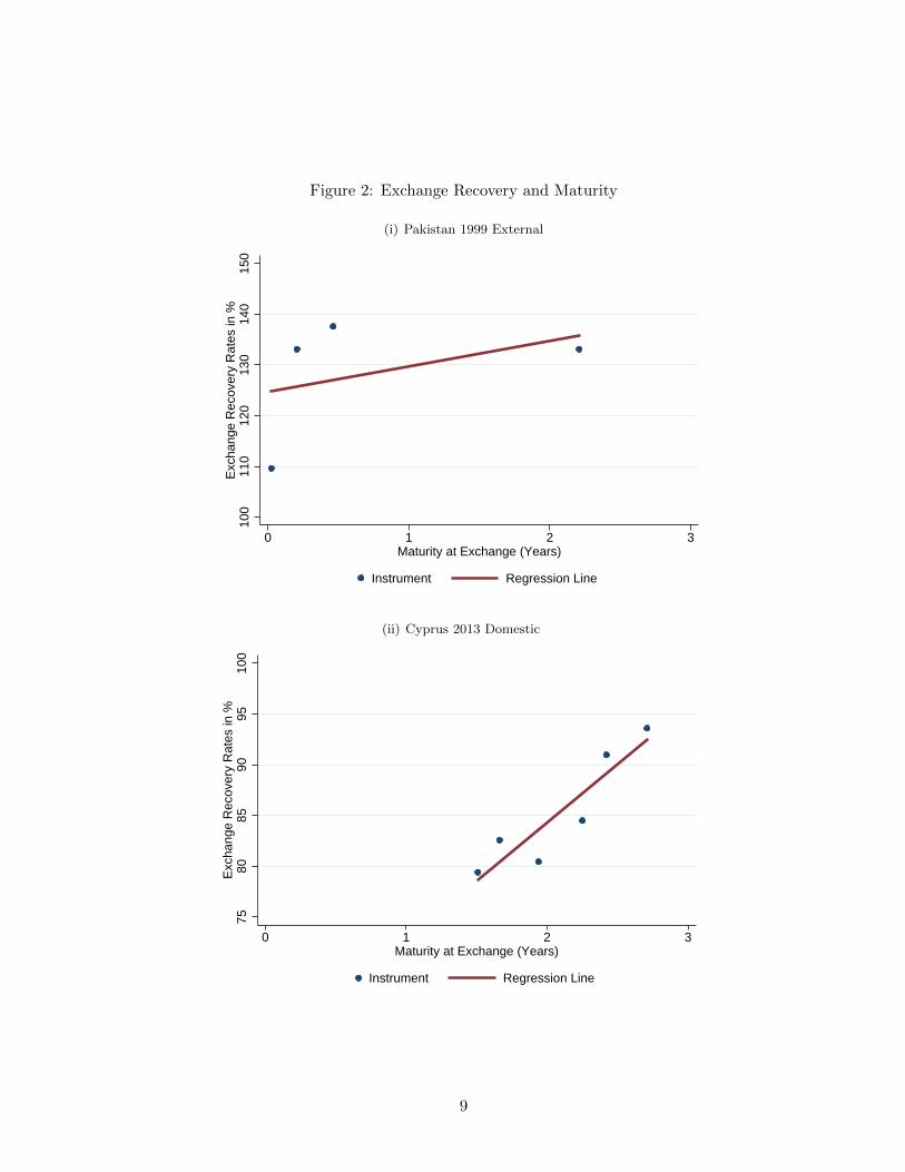
Figure 2: Exchange Recovery and Maturity
(i) Pakistan 1999 External100
110
120
130
140
150
Exchange R
ecovery
Rate
s in %
0 1 2 3Maturity at Exchange (Years)
Instrument Regression Line
(ii) Cyprus 2013 Domestic
75
80
85
90
95
100
Exchange R
ecovery
Rate
s in %
0 1 2 3Maturity at Exchange (Years)
Instrument Regression Line
9

Table 2 provides econometric support for the stylized fact. It reports the results of a cross-
sectional regression of the recovery rate (measured according to SZ or our measure) on maturity
as well as additional instrument- and episode-specific controls:
RecoverRateij = c+ β1Maturityij + β2xij + β3yj + cj + εi,j (3)
Here, Maturityij denotes the remaining maturity of instrument i at the date of exchange in
restructuring episode j; xij is a vector of instrument-specific variables, such as the coupon rate,
a dummy in case of a floating coupon rate, a dummy for the type of amortization profile (amorti-
zation only at maturity, [“bullet”] vs. already before maturity); yj is a vector of episode-specific
variables, such as the duration of the restructuring and the type of debt (domestic or external);
and cj is an episode-specific fixed effect.
The main result reported in Table 2 is that the effect of maturity on recovery rates (both
according to SZ and our measure) is positive and significant at the 1-percent level. Quantita-
tively, the effect is significant as well: on average, the recovery rate on a 10-year bond is 3–12
percentage points higher than on a 1-year bond. Columns (2) and (4) also reveal the effects
of other controls. Instruments with high fixed coupon rates or with floating rates experience
smaller recovery rates. The sign of the effect of the amortization profile is not precisely esti-
mated. Because of different sample sizes, the effect of restructuring duration on the recovery
rate only is identified in specification (2); the former is positive and significant.
10

Table 2: Cross-sectional Regression Results
SZ Recovery SZ Recovery Exchange ExchangeRate Rate, with Recovery Rate Recovery Rate,
controls (announcement) with controls
(1) (2) (3) (4)
coef/se coef/se coef/se coef/se
Maturity of Instrument (years) 0.30*** 0.35*** 1.03*** 1.24***(0.08) (0.08) (0.30) (0.29)
Coupon Rate (fixed, percent) -0.89*** -3.08***(0.18) (0.79)
Coupon Rate (float, dummy) -8.69*** -32.23***(1.95) (11.80)
Amortization Profile (payment before maturity, dummy) 2.92* -14.07(1.70) (8.97)
Duration of Restructuring (years) 17.55**(8.44)
External Debt Restructuring (dummy) -2.43(5.47)
Contant 52.00*** 41.02*** 78.77*** 104.06***(0.55) (9.94) (2.64) (6.82)
Episode Fixed Effects Yes Yes Yes YesNumber of Countries 15 15 12 12Number of Restructurings 28 28 16 16Observations 449 447 111 111Adjusted R-Squared 0.035 0.262 0.112 0.247
The table reports results of fixed effects OLS regressions. The dependent variable is SZ recovery rate (columns
1 and 2) or Exchange recovery rate (columns 3 and 4) (in %). The main explanatory variable is maturity of
instrument at the time of exchange. The control variables are instrument-specific controls and restructuring-
specific controls. Significance levels denoted by *** p < 0.01, ** p < 0.05, * p < 0.10. All regressions include
restructuring-specific fixed effects. Robust standard errors in parentheses.
11

3.2 Bond Prices
Stylized fact 2: The difference in prices between short-term and longer-term bonds
decreases in the run-up to the debt exchange.
Figure 3 reports bond price differentials—prices of short-term bonds minus prices of longer-
term bonds. We present two episodes: (i) Ukraine 2000 external, and (ii) Greece 2011–2012
external. Figure A6 in Appendix D reports two additional episodes: Dominican Republic 2004–
2005 external (bonds) and Argentina 2001–2005 external. In all figures, grey bars indicate the
date of the announcement of restructuring. Both figures show that prices of short-term and
long-term bonds converge in the run-up to the exchange. The observed price dynamics are not
specific either to the type of debt (domestic or external) or the restructuring strategy (strictly
preemptive, weakly preemptive or post-default).9,10
9We exclude prices of bonds that are no longer traded on the market.10See Guscina et al. (2017) for two episodes of the flattening of the term structure prior to a distress event.
12

Figure 3: Bond Price Differentials
(i) Ukraine 2000 External
05
10
15
20
25
Price D
iffe
rential (S
hort
− L
ong)
−6 −5 −4 −3 −2 −1 0Time relative to Exchange Date (Months)
Instrument S−L Regression Line
(ii) Greece 2011–2012 External
05
10
15
20
25
30
Price D
iffe
rential (S
hort
− L
ong)
−11 −10 −9 −8 −7 −6 −5 −4 −3 −2 −1 0Time relative to Exchange Date (Months)
Instrument S−L Regression Line S−L
Instrument S−M Regression Line S−M
Note: Grey bars indicate the date of the announcement of restructuring.
13

Table 3 provides econometric support for this stylized fact. It reports results of panel regres-
sions of the bond price differential on time relative to exchange date and maturity differential
with additional instrument- and episode-specific controls:
∆PriceS/Lj,t = c+ β1Timej,t + β2∆Maturity
S/Lj + β3yj + εj,t (4)
where ∆PriceS/Lj,t = PriceShortj,t −PriceLongj,t and ∆Maturity
S/Lj = MaturityShortj −MaturityLongj
denote bond price differential and maturity differential between short-term bonds and long-term
bonds at time t in debt restructuring j respectively. Timej,t denotes the time span until the
exchange date (in months) at time t in debt restructuring j. yj denotes the same vector of
episode-specific controls as in Section 3.1.
The main result in Table 3 is that the price of short-term debt approaches the price of
longer-term debt from above during the run-up to the exchange. This effect is significant at
the 1-percent level, and quantitatively large: over 6 months the price difference diminishes
by 9 percentage points (relative to face value of 100). The second result concerns the size
of the bond price differential conditional on time: it increases with the maturity differential.
For instance, the price of a 1-year bond exceeds the price of a 10-year bond by 4 percentage
points. Once we decompose episode-specific fixed effects, we find that restructuring strategy
(strictly preemptive vs post-default) and type of debt (external vs domestic) enter as a significant
explanatory variable. Moreover, Argentina’s 2001–2005 external debt restructuring appears to
constitute an outlier in that ceteris paribus, the bond price differential was larger.
The speed of price convergence is approximately the same in the subsample of restructuring
episodes where the exchange involves a single menu of new instruments vs different menus, see
the results as reported in Table A3 in Appendix D.
14
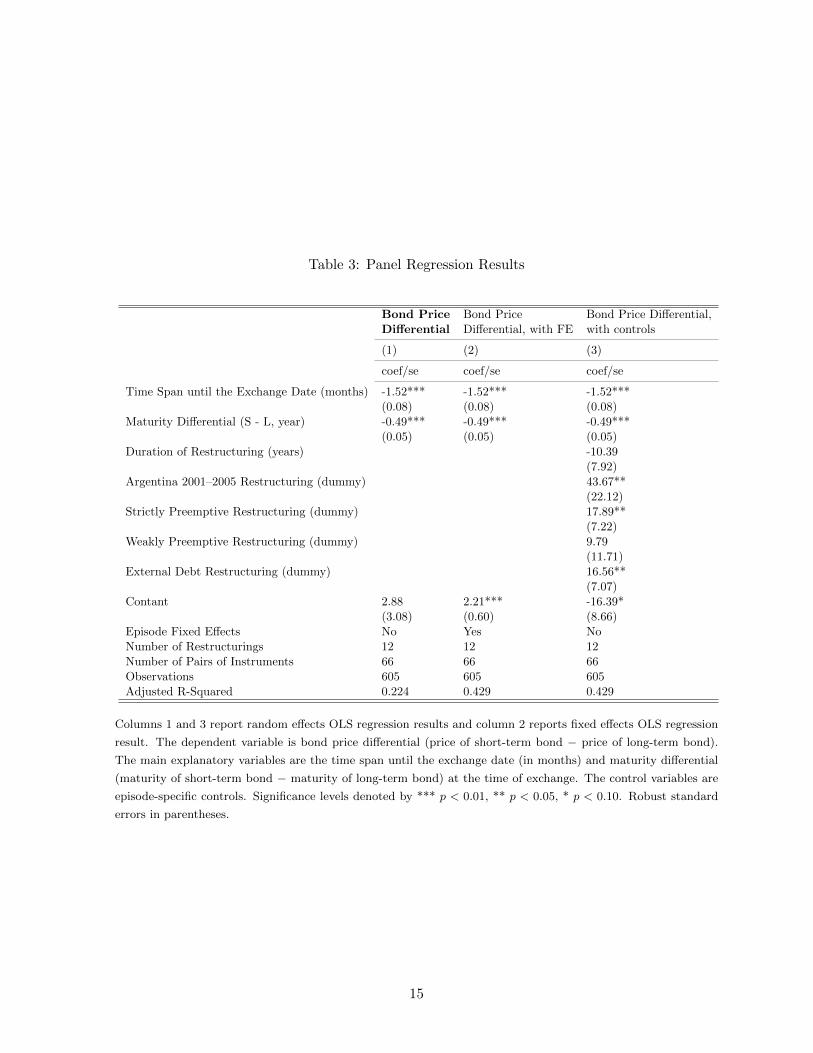
Table 3: Panel Regression Results
Bond Price Bond Price Bond Price Differential,Differential Differential, with FE with controls
(1) (2) (3)
coef/se coef/se coef/se
Time Span until the Exchange Date (months) -1.52*** -1.52*** -1.52***(0.08) (0.08) (0.08)
Maturity Differential (S - L, year) -0.49*** -0.49*** -0.49***(0.05) (0.05) (0.05)
Duration of Restructuring (years) -10.39(7.92)
Argentina 2001–2005 Restructuring (dummy) 43.67**(22.12)
Strictly Preemptive Restructuring (dummy) 17.89**(7.22)
Weakly Preemptive Restructuring (dummy) 9.79(11.71)
External Debt Restructuring (dummy) 16.56**(7.07)
Contant 2.88 2.21*** -16.39*(3.08) (0.60) (8.66)
Episode Fixed Effects No Yes NoNumber of Restructurings 12 12 12Number of Pairs of Instruments 66 66 66Observations 605 605 605Adjusted R-Squared 0.224 0.429 0.429
Columns 1 and 3 report random effects OLS regression results and column 2 reports fixed effects OLS regression
result. The dependent variable is bond price differential (price of short-term bond − price of long-term bond).
The main explanatory variables are the time span until the exchange date (in months) and maturity differential
(maturity of short-term bond − maturity of long-term bond) at the time of exchange. The control variables are
episode-specific controls. Significance levels denoted by *** p < 0.01, ** p < 0.05, * p < 0.10. Robust standard
errors in parentheses.
15

4 The Model
To identify potential drivers of the observed positive correlation between bond maturity and
recovery rate, we rely on a standard asset pricing model adapted to the sovereign debt context.
We establish two results. First, prior to the run-up to a debt restructuring prices of short-
term bonds exceed prices of longer-term bonds. When a restructuring episode ends with all
outstanding instruments being exchanged against the same new instrument (or basket of new
instruments), as is typically the case, then this first result implies the main stylized fact that
we have documented in Section 3: A higher haircut on short-term bonds. The first result
also explains the correlation between haircut and maturity if the haircut is measured following
Sturzenegger and Zettelmeyer’s approach. Second, in the run-up to a debt restructuring prices
of short- and longer-term bonds converge because default risk in the short-term rises. This
implies that the extent to which haircuts vary by maturity weakens as the restructuring event
approaches. Intuitively, successive bad news in the run-up to the restructuring compress price
differentials across maturities and as a consequence, the ex-post haircut differences diminish as
well.
4.1 Setup
To derive these results, consider a discrete time environment. In period t, a bond that matures
in period m either pays the predefined contractual payment, or the issuer announces a restruc-
turing.11 In the former case, the bond pays the contractual coupon, cm, if t < m; or the coupon
plus principal (unity) if t = m. In the latter case, the bond pays a recovery value, φmt . The
probability of no restructuring between periods t and s, s > t, given that no such restructuring
occurred until t, equals πt,s.
The timing of events in each period t is as follows: At the beginning of the period, investors
learn whether a restructuring “shock” has occurred, that is whether debt will be restructured
and thus pay off φmt . They may also receive new information about future restructuring risk
that may lead them to update their beliefs about πt,s. Conditional on the (new) information,
the bond pays the contractual payment or the recovery value, and in the former case the ex-
coupon price materializes.
To keep the notation simple, we assume that investors are risk neutral and the risk-free gross
interest rate is time invariant and equal to β−1. Standard asset pricing then implies that the ex-
coupon price equals the expected discounted price and coupon payment in the subsequent period
conditional on no restructuring, plus the expected discounted recovery value if a restructuring
shock hits in the subsequent period. Formally, letting pmt denote the ex-coupon price at date t
of a bond maturing at date m,
pmt = β{πt,t+1(cm + Et[p
mt+1|Nt+1]) + (1− πt,t+1)Et[φ
mt+1|At+1]} (5)
11For reasons outside the model (e.g., concerns about financial stability) Treasury bills and trade finances oftenare treated favorably in debt exchanges. In the empirical analysis, we exclude these instruments.
16

where Nt+1 and At+1 denote “no announcement of restructuring in period t + 1 (and earlier)”
and “announcement of restructuring in period t + 1,” respectively. In the last period before
maturity, t = m− 1, the equation holds with pmt+1 = 1.
4.2 First Result
Let ∆s,lt ≡ pst − plt denote the price difference between a short-term bond with maturity date
s and a longer-term bond with maturity date l.12 With identical coupons and recovery values
across bonds, cs = cl and φsi = φli for all i ≤ s, we have
∆s,lt = βs−tπt,s Et[∆
s,ls |Ns] (6)
That is, if a positive price difference is expected to prevail at date s—which holds true whenever
the longer-term bond is exposed to sufficiently high default risk after period s (or when it has
a sufficiently low coupon)—then the current price difference is positive as well. This positive
relationship between the current price difference and the expected future price difference only
collapses when the coupon or the recovery values of the longer-term bond are sufficiently large
relative to those of the short-term bond.
Absent major such differences between the coupons or the recovery values, long-term re-
structuring risk (and Et[∆s,ls |Ns] > 0) therefore implies ∆s,l
t > 0: Short-term bonds are more
expensive than longer-term bonds. This constitutes the first result stated before.
4.3 Second Result
Over time, ∆s,lt may change for two fundamentally different reasons. First, because time passes
by. And second, because news arrives, in particular about future restructuring risk. With
identical coupons and recovery values across bonds, the price difference evolves according to
∆s,lt+1 −∆s,l
t = βs−t−1πt+1,s|t+1 Et+1[∆s,ls |Ns]− βs−tπt,s|t Et[∆
s,ls |Ns] (7)
where the subscript of the probability of no restructuring now also indicates the information
set.13
Absent new information, the change in the price difference reduces to
∆s,lt+1 −∆s,l
t = βs−t−1πt+1,s|t+1 Et[∆s,ls |Ns](1− βπt,t+1|t) (8)
12This price difference is given by
∆s,lt ≡ β{πt,t+1(cs − cl + Et[∆
s,lt+1|Nt+1]) + (1− πt,t+1)Et[φ
st+1 − φl
t+1|At+1]}
= (cs − cl)s∑
i=t+1
βi−tπt,i +
s∑i=t+1
βi−tπt,i−1(1− πi−1,i)Et[φsi − φl
i|Ai] + βs−tπt,s Et[∆s,ls |Ns]
13That is, πt+1,s|t denotes the probability of no restructuring between periods t + 1 and s conditional oninformation at time t.
17

which is positive under the assumptions leading to the first result discussed above. That is,
absent new information prices further diverge.14
If new information implies sufficiently increased default risk in the short term, however, then
∆s,l may fall over time. Intuitively, an increase of short-term default risk proportionally lowers
the prices of short- and longer-term debt. In absolute terms, the price of short-term debt thus
falls more strongly.15 This constitutes the second result. It reflects the fact that lower expected
payoffs support lower contemporaneous prices. Note that the result continues to hold if new
information about recovery values arrives as long as the recovery values are identical for bonds
with different maturities.
4.4 Interpretation
By selecting episodes leading to restructuring we implicitly select episodes characterized by
rising short-term default risk. Ceteris paribus, the model predicts the price difference ∆s,l to be
positive during such episodes but decreasing over time. The positive price difference explains
the empirical finding of higher haircuts on shorter-term debt. The decreasing price difference
explains the empirical finding that the relation between maturity and haircut is weaker when
the restructuring is closer.
5 Default Probability Term Structure
We have argued in Section 4 that basic theory explains the two stylized facts—higher haircuts
on short-term bonds and smaller haircut differences with shorter window length—if short-term
default risk rises in the run-up to a restructuring. We now investigate empirically the relation
between bond prices and short-term default risk. In line with theory, we document an additional
stylized fact: in the run-up to an exchange the term structure of default risk becomes elevated
at the short end.
Stylized fact 3: The term structure of default probability becomes elevated at the
short end in the run-up to the exchange.
Using the method introduced in Ranciere (2002), we estimate the term structure of default risk.
In our estimation exercise, the main inputs are (a) the Credit Default Swap (hereafter CDS)
spread curve, and (b) the US Treasury bill yield curve proxying for the risk-free interest curve.
Following Ranciere (2002), we assume (i) no arbitrage, (ii) risk-neutrality, and (iii) the exchange
involving a single menu of new instruments for all restructured instruments.
Under these assumptions, we use annual yield curve data and linear interpolations to con-
struct estimates of the CDS spread curve for horizons between 1 and 120 months, at the monthly
frequency. Based on this, we use the no arbitrage condition to derive the forward default spread
14Deterministic price divergence may also result due to different coupons or expected recovery values (cs < cl
and φs < φl).15The price difference might also fall if the expected future price difference is updated downward.
18

curve. This curve measures the implied one-month ahead conditional default risk. Finally, we
use the risk-neutrality assumption and the fact that the exchange involves a single menu of new
instruments for all restructured instruments to derive the implied one-month ahead conditional
default probability. Appendix E discusses the details.
Figure 4 reports our conditional default probability estimates at the 1-year horizon. We
present two cases: (i) Ecuador 1999–2000 external and (ii) Greece 2011–2012 external. Figure
A8 in Appendix F reports the case of Argentina 2001–2005 external. In all figures, grey bars
indicate the date of the restructuring announcement. Both figures show that the conditional
short-term default probability (1 year) increases in the run-up to the exchange. This observed
rise is not specific to restructuring strategy (strictly preemptive, weakly preemptive or post-
default) and we also observe it at the 2-year and 3-year horizon, as reported in Table A4 in
Appendix F.
19

Figure 4: Default Probability Term Structure
(i) Ecuador 1999–2000 External
25
30
35
40
45
50
55
Defa
ult P
robabili
ty (
1−
year
horizon, %
)
−22 −21 −20 −19 −18 −17 −16 −15 −14 −13Time relative to Exchange Date (Months)
Short−term Default Probability
(ii) Greece 2011–2012 External
20
30
40
50
60
70
80
Defa
ult P
robabili
ty (
1−
year
horizon, %
)
−12 −11 −10 −9 −8 −7 −6 −5 −4 −3 −2 −1Time relative to Exchange Date (Months)
Short−term Default Probability
Note: Grey bars indicate the date of the announcement of restructuring.
20

Table 4: Panel Regression Results
Default Default Probability Default ProbabilityProbability 1–year 1–Year Horizon, 1–Year Horizon,Horizon(%) with FE with controls
(1) (2) (3)
coef/se coef/se coef/se
Time Span until the Exchange Date (months) 1.09*** 2,70*** 2.70***(0.26) (0.37) (0.37)
Duration of Restructuring (years) -3.11** -15.68***(1.43) (2.66)
Strictly Preemptive Restructuring (dummy) -37.98***(7.37)
Contant 61.20*** 71.92*** 115.36***(4.61) (4.06) (11.06)
Episode Fixed Effects No Yes NoNumber of Restructurings 3 3 3Number of Time Periods (months) 12 12 12Observations 36 36 36Adjusted R-Squared 0.373 0.628 0.628
Columns 1 and 3 report random effects OLS regression results and column 2 reports a fixed effects OLS regression
result. The dependent variable is the conditional default probability at the 1-year horizon (%). The main
explanatory variable is the time span until the exchange date (in months). The control variables are episode-
specific controls. Significance levels denoted by *** p < 0.01, ** p < 0.05, * p < 0.10. Robust standard errors in
parentheses.
Table 4 provides econometric support for the stylized fact. It presents results of panel
regressions of the conditional default probability at the 1-year horizon on the time span until
the exchange date with additional episode-specific controls:
Defaultj,t = c+ β1Timej,t + β2yj + εj,t (9)
where Defaultj,t denotes the conditional default probability over the 1-year horizon at time t
in debt restructuring j. Timej,t denotes the time span until the exchange at time t in debt
restructuring j. yj denotes the same vector of episode-specific controls as in Section 3.1.
The main result in Table 4 is that the conditional default probability increases in the run-up
to the exchange. This effect is significant at the 1-percent level, and quantitatively large: over 6
months the default risk increases by 7–16 percentage points. Once we decompose episode-specific
fixed effects, we find that restructuring strategy (strictly preemptive vs post-default) enters as
a significant explanatory variable. Duration of restructuring turns out to significantly reduce
the conditional default probability possibly because default probability gradually increases for
restructurings with longer duration.
21

6 Conclusion
This paper studies creditor losses (haircuts) across sovereign debt instruments during debt re-
structurings. We show that, contrary to conventional wisdom, creditors are not treated equally
in sovereign debt exchanges. We first construct a comprehensive dataset on instrument-specific
haircuts in recent sovereign debt restructuring episodes affecting private creditors. We demon-
strate that haircuts on shorter-term debt tend to be larger than those on longer-term debt,
and propose a simple asset pricing model that can theoretically explain this fact. We also
show that the data supports the causal link among short-term default risk, bond prices and
maturity-specific haircuts suggested by the model.
Our findings highlight a regularity that has not received much attention so far and has
potential implications for important dimensions of debt policy including, pari passu and its
limitations; the negotiation process during debt restructuring episodes; the value at risk of debt
securities of different maturities (and thus, of financial institutions that hold these instruments);
or the optimal debt management more broadly. However, further research is required before
drawing normative conclusions or policy prescriptions, as the findings in this paper do not allow
to conclude that specific bond maturities are better or worse than others for issuers or for
investors.
22
References
[1] Aguiar, M., and M. Amador, 2013, “Take the Short Route: How to Repay and Restructure
Sovereign Debt with Multiple Maturities,” NBER Working Paper No.19717.
[2] Arellano, C., and A. Ramanarayanan, 2012, “Default and the Maturity Structure in
Sovereign Bonds,” Journal of Political Economy, Vol.120(2), pp.187–232.
[3] Asonuma, T., and M.G. Papaioannou, 2016, ”Domestic Sovereign Debt Restructurings: Pro-
cesses, Outcomes and Challenges,” Manuscript, IMF.
[4] Asonuma, T., and C. Trebesch, 2016, “Sovereign Debt Restructurings: Preemptive or Post-
default,” Journal of European Economic Association, Vol.14(1), pp.175–214.
[5] Bedford, P., A. Penalyer, and C. Salmon, 2005, “Resolving Sovereign Debt Crises: The
Market-based Approach and the Role of the IMF,” Bank of England Financial Stability
Review, Vol.18(2), pp.91–100.
[6] Benjamin, D., and M.L.J. Wright, 2009, “Recovery Before Redemption? A Theory of Delays
in Sovereign Debt Renegotiations,” manuscript, UCLA.
[7] Broner, F.A., G. Lorenzoni, and S.L. Schmukler, 2013, “Why Do Emerging Economies Bor-
row Short Term?” Journal of the European Economic Association, Vol.11(1), pp.67–100.
[8] Chatterjee, S., and B. Eyigungor, 2012, “Maturity, Indebtness, and Default Risk,” American
Economic Review, Vol.102(6), pp.2674–2699.
[9] Cline, W.R, 1995, International Debt Reexamined. Washington DC: Institute for Interna-
tional Economics.
[10] Cruces, J., and C. Trebesch, 2013, “Sovereign Defaults: The Price of Haircuts,” American
Economic Journal: Macroeconomics, Vol.5(3), pp.85–117.
[11] Diaz-Cassou, J., A. Erce, and J. Vazquez-Zamora, 2008, “Recent Episodes of Sovereign Debt
Restructurings. A Case-study Approach,” Banco de Espana Occasional Paper No.0804.
[12] Eaton, J., and M. Gersovitz, 1981, “Debt with Potential Repudiation: Theoretical and
Empirical Analysis,” Review of Economic Studies, Vol.48(2), pp.289–309.
[13] Eichengreen, B., and R. Portes, 1986, “Debt and Default in the 1930s: Causes and Conse-
quences,” European Economic Review, Vol.30(3), pp.599–640.
[14] Eichengreen, B., and R. Portes, 1989, “After the Deluge: Default, Negotiation, and Read-
justment during the Interwar Years,” In The International Debt Crisis in Historical Perspec-
tive, edited by B. Eichengreen and P.H. Lindert, 12–47. Cambridge, MA: MIT Press.
[15] Fernandez, R., and A. Martin, 2014, “The Long and the Short of It: Sovereign Debt Crises
and Debt Maturity,” NBER Working Paper No.20786.
23

[16] Finger, H., and M. Mecagni, 2007, “Sovereign Debt Restructuring and Debt Sustainability:
An Analysis of Recent Cross-Country Experience,” International Monetary Fund (IMF)
Occasional Paper 255.
[17] Guscina, A., S. Malik, and M.G. Papaioannou, 2017, “Assessing Loss of Market Access,”
forthcoming IMF Working Paper.
[18] Hatchondo, J. C., and L. Martinez, 2009, “Long-duration Bonds and Sovereign Defaults,”
Journal of International Economics, Vol.79(1), pp.117–125.
[19] Hatchondo, J. C., L. Martinez, and C.S. Padilla, 2014, “Voluntary Sovereign Debt Ex-
changes,” Journal of Monetary Economics, Vol.61(C), pp.32–50.
[20] Hatchondo, J.C., L. Martinez, and C.S. Padilla, 2016, “Debt Dilution and Sovereign Default
Risk,” Journal of Political Economy, Vol.124(5), pp.1383–1422.
[21] Institute of International Finance (IIF), 2012, “Report of the Joint Committee on Strength-
ening the Framework for Sovereign Debt Crisis Prevention and Resolution,” IIF Principles
for Stable Capital Flows and Fair Debt Restructuring & Addendum, October 2012.
[22] Institute of International Finance (IIF), 2015, “Report on Implementation by the Principles
Consultative Group,” IIF Principles for Stable Capital Flows and Fair Debt Restructuring,
October 2015.
[23] International Monetary Fund (IMF), 2014, “Strengthening the Contractual Framework to
Address Collective Action Problems in Sovereign Debt Restructuring,” IMF Board Paper,
April 2014, available at https://www.imf.org/external/np/pp/eng/2014/090214.pdf.
[24] International Monetary Fund (IMF), 2015, “The Fund’s Lending Framework and
Sovereign Debt—Further Considerations,” IMF Board Paper, April 2015, available at
http://www.imf.org/external/np/pp/eng/2015/040915.pdf.
[25] Jeanne, O., 2009, “Debt Maturity and the International Finance Architecture,” American
Economic Review, Vol.99(5), pp.2135–2148.
[26] JP Morgan, 2000, “Introducing the J.P. Morgan Implied Default Probability Model: A
Powerful Tool for Bond Valuation,” September 2000.
[27] Lindert, P.H., and P.J.Morton, 1989, “How Sovereign Debt Has Worked,” In Developing
Country Debt and Economic Performance: The International Financial System, Vol.1, edited
by Jeffrey Sachs, pp.39–106. Chicago: University of Chicago Press.
[28] Niepelt, D., 2014, “Debt Maturity without Commitment,” Journal of Monetary Economics,
Vol.68(S), pp.S37–S57.
[29] Ranciere, R., 2002, “Credit Derivatives in Emerging Markets,” manuscript, IMF.
24

[30] Rieffel, L., 2003, Restructuring Sovereign Debt: The Case for Ad Hoc Machinery, Brooking
Institute Press.
[31] Rodrik, D., and A. Velasco, 1999, “Short-term Capital Flows,” In Annual World Bank
Conference on Development Economics, World Bank.
[32] Sturzenegger, F., and J. Zettelmeyer, 2006, Debt Defaults and Lessons from a Decade of
Crises, MIT Press.
[33] Sturzenegger, F., and J. Zettelmeyer, 2008, “Haircuts: Estimating Investors Losses in
Sovereign Debt Restructuring, 1998–2005,” Journal of International Money and Finance,
Vol.27(5), pp.780–805.
[34] Zettelmeyer,J., C. Trebesch, and M. Gulati, 2013, “The Greek Debt Restructuring: An
Autopsy,” Economic Policy, Vol.28(75), pp.513–563.
25

Appendix A Dataset: Selected Recent Restructurings
Table A1: Selected Recent Sovereign Debt Restructurings (1998–2015)
EpisodeAnnouncement Exchange Restructuring SZ Haircut Differential Maturity of Short-
of Default (Start) (End) Strategy (S- and L-term, percent) and Long-term Debt(years)
ExternalPakistan Jan-99 Dec-99 Strictly Preemptive 25.7 0 and 2.5Russia (PRINs & IANs) Nov-98 Aug-00 Post-Default 19.2 -0.1 and 10.9Ecuador Jan-99 Aug-00 Post-Default 28.2 1.7 and 24.5Uruguay Mar-03 May-03 Strictly Preemptive 8.4 0.5 and 24.2Argentina (Global Exchange) Nov-01 Jun-05 Post-Default 13.4 0.1 and 22.6Grenada Oct-04 Nov-05 Weakly Preemptive 21.4 0 and 13.0Belize Aug-06 Feb-07 Weakly Preemptive 22.4 0 and 8.0Greece Jul-11 Mar-12 Strictly Preempitve 45.4 0 and 28.5Saint Kitts and Nevis Jun-11 Apr-12 Weakly Preemptive 10.3 0 and 8
DomesticRussia (GKOs resident) Aug-98 May-99 Post-Default 2.4 -0.3 and 0.3Argentina (Phrase I) Oct-01 Nov-01 Strictly Preemptive 7.8 0.5 and 29.6Uruguay Mar-03 May-03 Strictly Preemptive 10.4 0.0 and 8.8Jamaica Feb-13 Mar-13 Strictly Preemptive 0.9 0 and 33.2Cyprus May-13 Jul-13 Strictly Preemptive 14.7 1 and 2.7
26

Appendix B Haircuts/Recovery Rates
Figure A1: SZ Recovery and Maturity
(i) Belize 2006–2007 External60
65
70
75
80
85
90
SZ
Recovery
in %
0 2 4 6 8 10Maturity at Exchange (Years)
Instrument Regression Line
(ii) Saint Kitts and Nevis 2011–2012 Domestic
20
25
30
35
40
45
SZ
Recovery
in %
−5 0 5 10Maturity at Exchange (Years)
Instrument Regression Line
27

Figure A2: Exchange Recovery and Maturity
(i) Greece 2011–2012 External20
30
40
50
60
70
Exchange R
ecovery
Rate
s in %
0 10 20 30Maturity at Exchange (Years)
Instrument Regression Line
(ii) Urugauy 2003 Domestic
60
70
80
90
100
110
120
130
Exchange R
ecovery
Rate
s in %
0 2 4 6 8 10Maturity at Exchange (Years)
Instrument Regression Line
28

Figure A3: Exchange Recovery and Maturity at Different Points of Time
(i) Pakistan 1999 External — 6 months before the announcement70
80
90
100
110
120
Exchange R
ecovery
in %
0 1 2 3Maturity at Exchange (Years)
Instrument Regression Line
(ii) Pakistan 1999 External — 6 months after the announcement
80
90
100
110
120
130
Exchange R
ecovery
in %
0 1 2 3Maturity at Exchange (Years)
Instrument Regression Line
29

(iii) Greece 2011–2012 External — 6 months before the announcement
20
30
40
50
60
70
Exchange R
ecovery
in %
0 10 20 30Maturity at Exchange (Years)
Instrument Regression Line
(iv) Greece 2011–2012 External — 6 months after the announcement
50
60
70
80
90
100
110
Exchange R
ecovery
in %
0 10 20 30Maturity at Exchange (Years)
Instrument Regression Line
30

Table A2: Cross-sectional Regression Results
Exchange Exchange Exchange ExchangeRecovery Rate Recovery Rate, Recovery Rate Recovery Rate,(6 months before with controls (6 months after with controlsannouncement) (announcement)
(1) (2) (3) (4)
coef/se coef/se coef/se coef/se
Maturity of Instrument (years) 0.54** 0.54** 5.74*** 5.79***(0.24) (0.24) (1.74) (1.81)
Coupon Rate (fixed, percent) -0.76 0.86(0.64) (4.95)
Coupon Rate (float, dummy) -11.31 4.53(9.18) (74.22)
Amortization Profile (payment before maturity, dummy) -13.61* 33.03(7.12) (56.42)
Duration of Restructuring (years)
External Debt Restructuring (dummy)
Contant 68.70*** 76.68*** 80.04*** 71.25(1.89) (5.64) (15.31) (42.88)
Episode Fixed Effects Yes Yes Yes YesNumber of Countries 12 12 12 12Number of Restructurings 16 16 16 16Observations 104 104 111 111Adjusted R-Squared 0.054 0.118 0.104 0.108
The table reports results of fixed effects OLS regressions. The dependent variable is Exchange recovery rate (in
%). The main explantory variable is maturity of instrument at the time of exchange. Columns 1 and 2 report
results for Exchange recovery rate 6 months before the announcement and columns 3 and 4 report results for
Exchange recovery rate 6 months after the announcement. The control variables are instrument-specific controls
and restructuring-specific controls. Significance levels denoted by *** p < 0.01, ** p < 0.05, * p < 0.10. All
regressions include restructuring-specific fixed effects. Robust standard errors in parentheses.
31

Appendix C SZ Haircuts Robustness Check
One advantage of the SZ haircut measure is that it is relatively robust to the posited exit yield of
new instruments because both the cash flows of old and new instruments are discounted at the
same yield. However, there still remains the question when the exit yield should be measured.
To address this concern, we conduct a robustness check and recompute haircuts for higher (exit
yield +1 percent) and lower (exit yield -1 percent) yields.
Figure A4 and A5 report results for Dominica 2003–2004 domestic and Belize 2006–2007
external, respectively. In both cases, SZ recovery rates on short-term debt are lower than those
on long-term debt whichever yield is used.
32
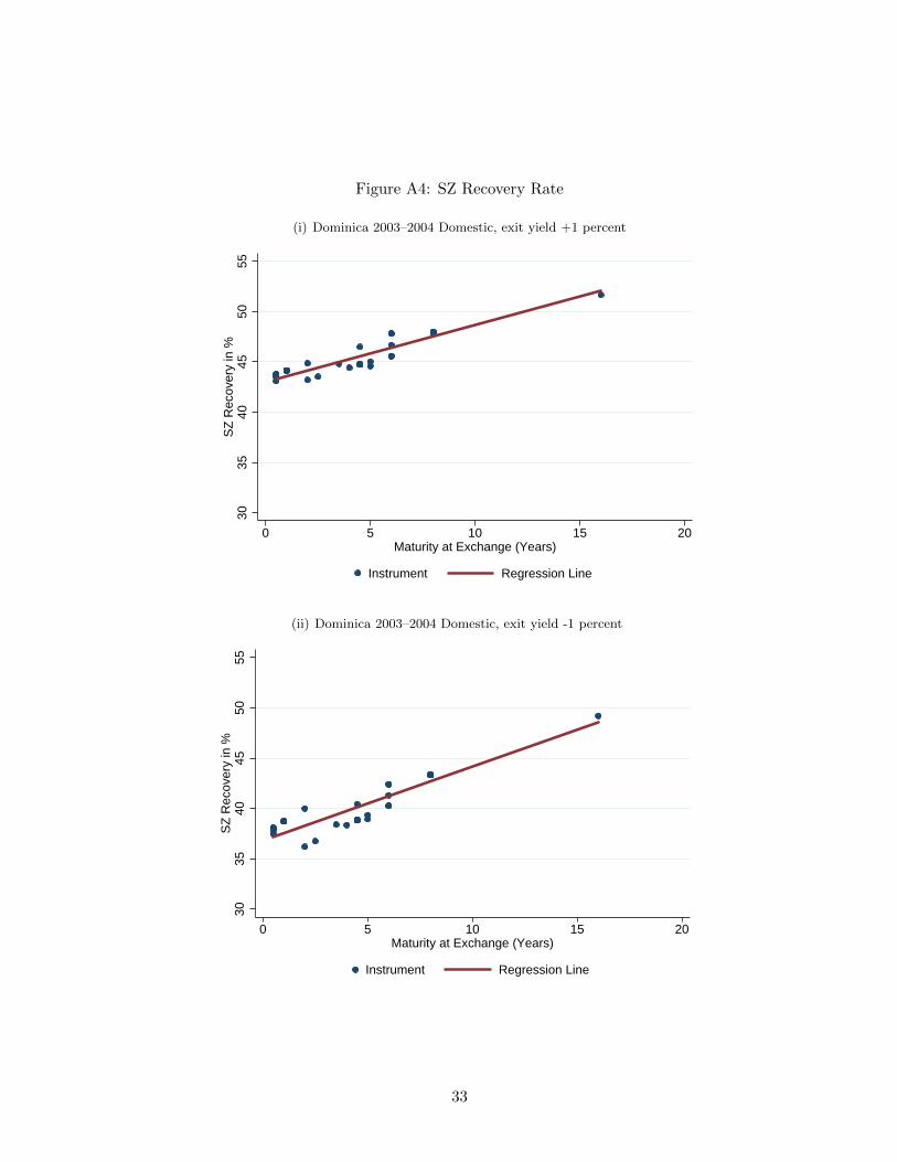
Figure A4: SZ Recovery Rate
(i) Dominica 2003–2004 Domestic, exit yield +1 percent30
35
40
45
50
55
SZ
Recovery
in %
0 5 10 15 20Maturity at Exchange (Years)
Instrument Regression Line
(ii) Dominica 2003–2004 Domestic, exit yield -1 percent
30
35
40
45
50
55
SZ
Recovery
in %
0 5 10 15 20Maturity at Exchange (Years)
Instrument Regression Line
33

Figure A5: SZ Recovery Rate
(i) Belize 2006–2007 External, exit yield +1 percent60
65
70
75
80
85
90
SZ
Recovery
in %
0 2 4 6 8 10Maturity at Exchange (Years)
Instrument Regression Line
(ii) Belize 2006–2007 External, exit yield -1 percent
65
70
75
80
85
90
95
SZ
Recovery
in %
0 2 4 6 8 10Maturity at Exchange (Years)
Instrument Regression Line
34

Appendix D Bond Prices
Figure A6: Bond Price Differentials
(i) Dominican Republic 2004–2005 External (bonds)0
510
15
20
25
30
35
40
45
Price D
iffe
rential (S
hort
− L
ong)
−16 −15 −14 −13 −12 −11 −10 −9 −8 −7 −6 −5 −4 −3 −2 −1 0Time relative to Exchange Date (Months)
Instrument S−L Regression Line
(ii) Argentina 2001–2005 External
05
10
15
20
25
30
Price D
iffe
rential (S
hort
− L
ong)
−7 −6 −5 −4 −3 −2 −1 0Time relative to Exchange Date (Months)
Instrument S−L Regression Line S−L
Instrument S−M Regression Line S−M
Note: Grey bars indicate the date of the announcement of restructuring.
35

Table A3: Panel Regression Results
Bond Price Bond Price Bond Price Bond PriceDifferential, Differential, Differential, Differential,Symmetric Symmetric, Non-Symmetric Non-Symmetric,
with controls with controls
(1) (2) (3) (4)
coef/se coef/se coef/se coef/se
Time Span until Exchange Date (months) -1.42*** -1.43*** -1.79*** -1.81***(0.09) (0.10) (0.15) (0.15)
Maturity Differential (S - L, year) -0.51*** -0.40*** 0.34 0.81***(0.05) (0.05) (0.24) (0.22)
Duration of Restructuring (years) -37.95*** -29.37***(2.41) (4.25)
Argentina 2001–2005 restructuring (dummy)
Strictly Preemptive Restructuring (dummy) -114.63*** 19.75***(7.23) (2.02)
Weakly Preemptive Restructuring (dummy) -15.74***(5.98)
External Debt Restructuring (dummy) 17.43*** 48.69***(1.56) (5.11)
Contant 7.81** 127.09*** 1.05 -18.02***(3.70) (7.72) (5.46) (2.74)
Episode Fixed Effects No No No NoNumber of Restructuirngs 6 6 6 6Number of Pairs of Instruments 51 51 15 15Observations 487 487 118 118Adjusted R-Squared 0.190 0.403 0.289 0.787
The table reports results of random effects OLS regressions. The dependent variable is bond price differential
(price of short-term bond - price of long-term bond). The main explanatory variables are the time span until the
exchange date (in months) and maturity differential (maturity of short-term bond - maturity of long-term bond)
evaluated at the time of exchange. Columns 1 and 2 report regression results for restructurings with exchanges
involving a single menu of new instruments. Columns 3 and 4 report regression results for restructurings with
exchanges involving different menus of new instruments. The control variables are episode-specific controls.
Significance levels denoted by *** p < 0.01, ** p < 0.05, * p < 0.10. Robust standard errors in parentheses.
36

Appendix E Estimation of Term Structure of Default Risk
We follow Ranciere (2002).
1st Step: Constructing the monthly yield curve
We interpolate the annual yield curve linearly for both (i) CDS spreads and (ii) risk-free
interest rates as follows:
CDSM,jt = CDSA,i
t +j − i12
(CSDA,i+12t − CDSA,i
t )
RFM,jt = RFA,i
t +j − i12
(RFA,i+12t −RFA,i
t ) (A1)
for i = 0, 12, 23, 36, ..., 108 and j = i+ 1, i+ 2, ..., i+ 11
The annual yield for 0-year horizon is assumed to be zero; CDSA,0t = RFA,0
t = 0.
where CDSM,jt and RFM,j
t denote estimated monthly CDS spreads and risk-free interest rates,
respectively. CDSA,it and RFA,j
t denote observed annual CDS spreads and risk-free interest
rates, respectively.
2nd Step: Computing a forward default spread curve
We apply the no arbitrage condition to derive the forward default spread curve (in month
1,2,3,...., 120) as follows:
(1 +RFM,h,jt + CDSM,h,j
t ) = (1 +RFM,jt + CDSM,j
t )/(1 +RFM,ht + CDSM,h
t ) (A2)
for i = 1, 2, 3, ..., 120 and h = j − 1
where CDSM,h,jt and RFM,h,j
t denote estimated forward default spreads and forward risk-free
interest rates, respectively. The forward default spread measures the implied one-period ahead
conditional default risk.
3rd Step: Computing the term structure of conditional default probabilities
We use risk-neutrality and the fact that the exchange involves a single menu of new instru-
ments for all restructured instruments to derive the implied one-period ahead conditional default
risk:
(1 +RFM,h,jt ) = (1− P h,j
t ) ∗ (1 +RFM,h,jt + CDSM,h,j
t ) + P h,jt ∗ Rt
s.t. Rt = argmin1
n
n∑i=1
{pit − pit({RFM,k,k+1t }H−1k=h , P
j,ht , Rt)}2 (A3)
for j = 1, 2, 3, ..., 120 and h = j − 1
37

where P h,jt and Rt are implied one-period ahead conditional default probability and time variant
recovery. The implied time-variant recovery is estimated to minimize mean squared deviations of
the estimated bond prices pit({RFM,k,k+1t }H−1k=h , P
j,ht , Rt)—based on inputs of streams of risk-free
interest rates until maturity, estimated conditional default risk and time-variant recovery—from
the observed price pit. This implied time-variant recovery converges to the observed nominal
recovery at the time of exchange as reported in Figure A7.16
16JP Morgan (2000) proposes an alternative approach to compute implied recovery rates.
38

Figure A7: Implied Nominal Recovery Rate
(i) Ecuador 1999–2000 External
40
45
50
55
60
65
70
75
80
Implie
d N
om
inal R
ecovery
Rate
(%
)
−22 −21 −20 −19 −18 −17 −16 −15 −14 −13Time relative to Exchange Date (Months)
Implied Recovery Rate
(ii) Greece 2011–2012 External
20
30
40
50
60
70
Implie
d N
om
inal R
ecovery
Rate
(%
)
−12 −11 −10 −9 −8 −7 −6 −5 −4 −3 −2 −1Time relative to Exchange Date (Months)
Implied Recovery Rate
Note: Grey bars indicate the date of the announcement of restructuring.
39
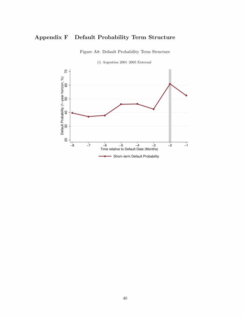
Appendix F Default Probability Term Structure
Figure A8: Default Probability Term Structure
(i) Argentina 2001–2005 External20
30
40
50
60
70
Defa
ult P
robabili
ty (
1−
year
horizon, %
)
−8 −7 −6 −5 −4 −3 −2 −1Time relative to Default Date (Months)
Short−term Default Probability
40
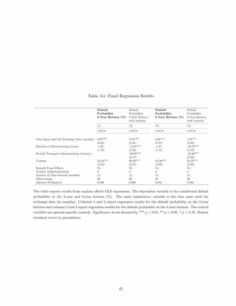
Table A4: Panel Regression Results
Default Default Default DefaultProbability Probability Probability Probability2-Year Horizon (%) 2-Year Horizon, 3-Year Horizon (%) 3-Year Horizon,
with controls with controls
(1) (2) (3) (4)
coef/se coef/se coef/se coef/se
Time Span until the Exchange Date (months) 0.87*** 2.16*** 0.68*** 1.87***(0.22) (0.31) (0.21) (0.30)
Duration of Restructuring (years) -1.86 -12.01*** -1.40 -10.72***(1.19) (2.23) (1.14) (2.19)
Strictly Preemptive Restructuring (dummy) -30.69*** -28.20***(6.17) (6.06)
Contant 52.56*** 96.28*** 48.28*** 88.45***(3.83) (9.27) (3.65) (9.09)
Episode Fixed Effects No No No NoNumber of Restructurings 3 3 3 3Number of Time Periods (months) 12 12 12 12Observations 36 36 36 36Adjusted R-Squared 0.336 0.606 0.252 0.543
The table reports results from random effects OLS regressions. The dependent variable is the conditional default
probability at the 2-year and 3-year horizon (%). The main explanatory variable is the time span until the
exchange date (in months). Columns 1 and 2 report regression results for the default probability at the 2-year
horizon and columns 3 and 4 report regression results for the default probability at the 3-year horizon. The control
variables are episode-specific controls. Significance levels denoted by *** p < 0.01, ** p < 0.05, * p < 0.10. Robust
standard errors in parentheses.
41