NBER WORKING PAPER SERIES

ASSET PRICE VOLATILITY,BUBBLES AND PROCESS SWITCHING

Robert P. Flood

Robert J. Hodrick

Working Paper No. 1867

NATIONAL BUREAU OF ECONOMIC RESEARCH1050 Massachusetts Avenue

Cambridge, MA 02138March 1986

The research reported here is part of the NBER's research programin Financial Markets and Monetary Economics. Any opinionsexpressed are those of the authors and not those of the NationalBureau of Economic Research.

NBER Working Paper #186 7Mardi 1986

Asset Price Volatility, Bubbles and Process Switdiing

ABSTRZCT

Evidence of excess volatilities of asset prices compared with those of

market fundamentals is often attributed to speculative bubbles. This study

examines the sense in which speculative bubbles could in theory lead to excess

volatility, hut it demonstrates that some of the variance hounds evidence

reported to date precludes bubbles as a reason why asset prices might violate

such hounds. The findings must represent some other model misspecffication or

market inefficiency. One important misspecification occurs when the

researcher incorrectly specifies the time series properties of market

fundamentals. A bubble—free example economy characterized by a potential

switch in government policies produces paths of asset prices that would

appear, to an unwary researcher, to contain bubbles.

Robert P. Flood Robert J. Hodrickflepartment of Economics Kellogg Graduate SchoolNorthwestern University of ManagementEvanston, IL 60201 Northwestern University

Evanston, IL 60201

—1—

The introduction and use of variance hounds tests by financial economists

interested in asset pricing and market efficiency has generated considerable

controversy. The first tests postulated a simple model in which market

efficiency required assets to have a constant expected real rate of return.

The apparent strong rejection of this hypothesis in the work of Shiller

(l9Rla, 1981h) and particularly Grossman and Shiller (1981) was followed

quickly by a number of different responses. The statistical properties of the

tests in small samples and the time series assumptions of the data were

criticized)- Substantial resources have also been devoted to complications of

the model that allow time variation in discount rates and risk premiums, while

remaining within the representative agent pardigm.2 Others have taken the

performance of the simple model and the excess volatility of asset prices

described in the tests to be indicative of market inefficiency.

One particular type of market inefficiency that receives much attention

in these discussions is that asset markets may be characterized by speculative

bubbles. Representative of these statements is Ackley's (193, p. 13)

discussion of Shiller's (1981a, 1981h) findings, in which he states, "But,

surely, it is possible that speculative price bubbles, upward or downward,

., supply part of the explanation." Similarly, in Fischer's (1q84, p. 500)

discussion of SMiler (1984', he states, "Backing up that empirical evidence

was the development, by Shiller and others, of the theory of speculative

bubbles, providing a reason that prices could fluctuate excessively without

smart investors being able to profit from knowing they were living in a

bubble." Similar statements have been made by others in discussions of stock

price volatility and in discussions of the volatility of foreign exchange

rates

—2—

In this paper we examine whether some of the variance hounds tests

reported to date can he evidence for the hypothesis that asset prices contain

speculative bubbles. The speculative bubbles discussed here are of the type

studied by Flood and Garber (1980) and Blanchard and Watson (1982). The

variance bounds tests we discuss are of the types that were conducted by

Shiller (1981a, 1°81h, 1982, 1984) and l4ankiw, Romer and Shapiro (1985) and

that were discussed by Grossman and Shilier (1981). We demonstrate the sense

in which the existence of bubbles can in theory lead to excess volatility of

asset prices relative to the volatility of market fundamentals, hut we explain

why certain variants of variance bounds tests preclude hubbies as a reason why

asset prices might violate such hounds. This result, without its formal

demonstration, is mentioned by Mankiw, Romer and Shapiro (1985, p. 681) who

state, "the inequalities ... hold even if there are bubbles." Since many

researchers have mentioned bubbles as a possible reason for the failure of the

simple rational expectations model in variance bounds tests, we thought it

worthwhile to elaborate on the remark in Mankiw, Romer and Shapiro (1985).

The issue turns on how one measures the inherently unobservable construct

that Shiller (1981a) denoted the ex post rational price. If one uses the

sample's terminal market price to construct a measurable counterpart to ex

post rational price, as is done by Shiller (1982, 1984), Grossman and Shiller

(1981) and Mankiw, Romer and Shapiro (1985), failure of a variance bounds test

cannot he attributed to the existence of speculative bubbles. The reason is

that use of the sample market price effectively builds bubbles into the null

hypothesis. Rejection of the null must consequently he due to other

sources. Potential explanations include small sample properties of the tests,

general misspecification of the model and failure of the data to satisfy the

ergodicity assumption implicit in the use of the statistics.4

—3—

In bubble research one particularly important misspecification of the

model occurs when the researcher incorrectly specifies the time series

properties of market fundamentals. The second purpose of this paper is to

explain, in terms of a simple model economy, how anticipated changes in market

fundamentals may produce asset price paths that would appear to an empirical

researcher, who is unaware of the potential change, to he characterized by

bubbles even though the economy is bubble free. The example economy is

described by a potential change in government policies that we label a process

switch.

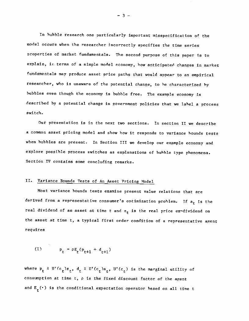
Our presentation is in the next two sections. In section II we describe

a common asset pricing model and show how it responds to variance hounds tests

when hubbies are present. In Section III we develop our example economy and

explore possible process switches as explanations of bubble type phenomena.

Section IV contains some concluding remarks.

TI. Variance Bounds Tests of An Asset Pricing Model

Most variance hounds tests examine present value relations that are

derived from a representative consumer's optimization problem. If at is the

real dividend of an asset at time t and z is the real price ex—dividend on

the asset at time t, a typical first order condition of a representative agent

requires

(1) Pt = PE(P+i +

where Pt U'(c)z, d E U'(c'a, U'(c) is the marginal utility of

consumption at time t, p is the fixed discount factor of the agent

and E(.) is the conditional expectation operator based on all time t

—4—

information. Equation (1) requires that the utility of the real value

sacrificed by the individual in purchasing the asset he equal to the

conditional expectation of the utility of the real value of the benefit from

holding and selling the asset.

Equation (1) has the form of a linear difference equation that arises in

many rational expectations models. Hence, a solution that depends only on

market fundamentals can he written as

(2) f =

and substitution of (2) into (1) with equality of p and Pt requires A = p1.

Notice that If (1) is postulated as the entire model, an additional

arbitrary element, ht, can he added to the market fundamentals solution to

provide an alternative solution,

(3) Pt = P1E(d+1) + b.

The model requires only that the sequence of he's possess the property that

(4) E(b+i) = Pbt, i =

since with this property the solution (3) satisfies (1). The time series

is termed a rational bubble according to Flood and (arher (l9O), since it

satisfies the Euler equation (1). Absence of bubbles requires that each

element of the sequence is zero.5 The time series property of bubbles

described by (4) assures that bubbles cannot be a reason that the Euler

—5—

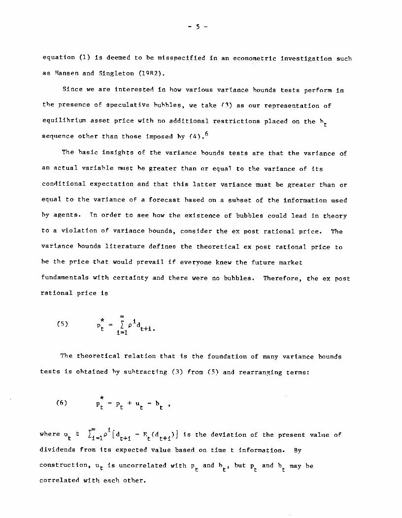
equation (1) is deemed to he misspecified in an econometric Investigation such

as Hansen and Singleton (1952).

Since we are interested in how various variance hounds tests perform in

the presence of speculative bubbles, we take (3) as our representation of

equilibrium asset price with no additional restrictions placed on the ht

sequence other than those imposed fr (4)6

The basic insights of the variance bounds tests are that the variance of

an actual variable must he greater than or equal to the variance of its

conditional expectation and that this latter variance must be greater than or

equal to the variance of a forecast based on a subset of the Information used

by agents. in order to see how the existence of bubbles could lead in theory

to a violation of variance hounds, consider the ex post rational price. The

variance hounds literature defines the theoretical ex post rational price to

he the price that would prevail If everyone knew the future market

fundamentals with certainty and there were no bubbles. Therefore, the ex post

rational price is

(5) p =

The theoretical relation that is the foundation of many variance bounds

tests is obtained by subtracting (3) from (5) and rearranging terms:

(6) =Pt + u — ht

i

where u = {d1 —Et(dt÷i)] is the deviation of the present value of

dividends from its expected value based on time t information. By

construction, u is uncorrelated with and ht, but p and h may he

correlated with each other.

—6—

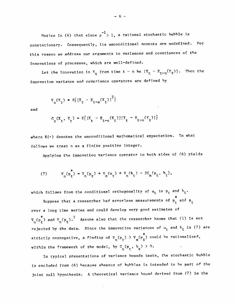
Notice in (4) that since p—i> 1, a rational stochastic bubble is

nonstationary. Consequently, its unconditional moments are undefined. For

this reason we address our arguments to variances and covariances of the

innovations of processes, which are well—defined.

Let the innovation in from time t — n he [X — E_(Xt)J. Then the

innovation variance and covarlance operators are defined by

V(X) = E{ [X — E(Xt) i2

and

C (X , Y )= — E (X )][Y — E (Y )j}

n t t t t—n t t t—n t

where E() denotes the unconditional mathematical expectation. In what

follows we treat n as a finite positive integer.

Applying the innovation variance operator to both sides of (6) yields

(7) V(p) = V(p) + V(ut) + V(b) — 2C(p, bt),

which follows from the conditional orthogonality of Ut to Pt and bt.

Suppose that a researcher had errorless measurements of p and Pt

over a long time series and could develop very good estimates of

V(p) and V(p).7 Assume also that the researcher knows that (1) is not

rejected by the data. Since the innovation variances of u and ht in (7) are

strictly nonnegative, a finding of V(p) > V(p) could he rationalized,

within the framework of the model, by c(p, h) > 0.

In typical presentations of variance hounds tests, the stochastic bubble

is excluded from (6) because absence of hubbies is intended to he part of the

joint null hypothesis. A theoretical variance bound derived from (7) in the

—7—

absence of bubbles is V(p) > V(pt). It is easy to construct examples in

which a sufficiently large innovation variance in b causes this variance

bound to he violated. Consider the situation in which the innovations in ht

are orthogonal to the innovations in market fundamentals. In this case,

= V(h). Therefore, the right—hand side of (7) reduces

to V(p) + V(ut) — V(h), and a sufficiently large innovation variance in

the bubble could cause V(P) < V(Pt).8

We imagine that theoretical exercises similar to the above have spawned

the popular argument that the failure of variance hounds tests can he due to

speculative hubbies. Analogously, it has been argued that failure to reject

the variance bounds inequalities is due to exclusion from the sample of time

periods containing bubbles.9 We now demonstrate that this theoretical

intuition is not correct in all situations. The practical implementation of

- many variance bounds tests precludes rational stochastic bubbles, per Se, as

the explanation for the failure of the test.

The difference between the theoretical exercise described above and its

practical implementation arises, of course, in the constuction of an

observable counterpart to Pt. In practice it is impossible to measure the

ex post rational price because it depends on the infinite future. Researchers

therefore typically measure a related variable denoted Since actual price

and dividend data are available for a sample of observations on t =

researchers use

..

—T—t

T—t(8) p= Pd+i+P T' t=O,•',T—l,

1=1

in place of Notice from (5) and (5) that

—8—

* T_t* T—t(9a) Pt=Pt•_p

which implies from () that

* T—t(9h) Pt = Pt + p (bT — UT).

Since UT is the innovation in the present value of dividends between time T

and the infinite future, it is uncorrelated with all elements of the time T

information set which includes time t information. Since hT depends on the

evolution of the stochastic bubble between t and T, it is not orthogonal to

time t information.

Notice what happens when (9h) is solved for Pt and the result is

substituted into (6). After slight rearrangement, one obtains

(10) Pt = Pt + w,

where

(11) w E u — T_t) + (pTtb — he).

quation (10) is the empirical counterpart of (6) and forms the basis of the

usual variance hounds tests. The only important difference between our

version of (10) and that of previous researchers is that we have explicitly

allowed for rational stochastic bubbles in our derivation.

—9—

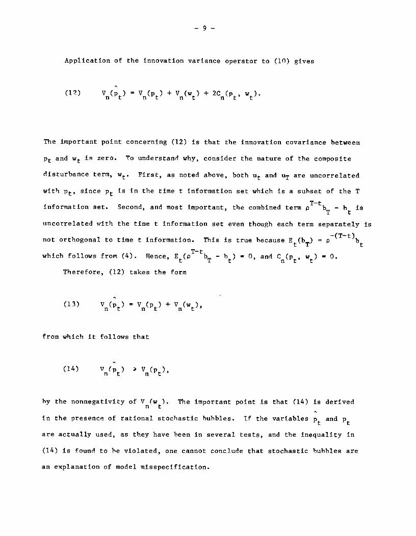
Application of the innovation variance operator to (10) gives

(l) v(;) = V(p) + V(w) + 2C(P, we).

The important point concerning (12) is that the innovation covariance between

Pt and Wt is zero. To understand why, consider the nature of the composite

disturbance term, w. First, as noted above, both Ut and UT are uncorrelated

with p1, since is in the time t information set which is a subset of the T

information set. Second, and most important, the combined term PT_tb — bt is

uncorrelated with the time t information set even though each term separately is

not orthogonal to time t Information. This is true because Et(hT) = t)b

which follows from (4). Hence, Et(pT tbT — h) = 0, and w) 0.

Therefore, (12) takes the form

(13) V(;) = V(p) +

from which it follows that

(14)

by the nonnegativity of V(w). The important point is that (14) is derived

in the presence of rational stochastic bubbles. If the variables Pt and

are actually used, as they have been in several tests, and the inequality in

(14) is found to he violated, one cannot conclude that stochastic hubbies are

an explanation of model misspecification.

— 10 —

Of course, research that does not use the terminal price T to

construct Pt does not discriminate among possible reasons for rejection of the

null hypothesis. The research which does use the actual terminal market price

therefore incorporates one of the alternative hypotheses into the null

hypothesis. While this may make it more difficult to reject the null

hypothesis, a reversal of the inequality in (14) cannot he attributed to

rational stochastic bubbles.

ha. The Mankiw, Romer, Shapiro Test

Flavin (1983) and Kleidon (1985b) argued that estimation of the sample

variance by subtraction of the sample mean rather than the population mean

produces small sample bias in variance hounds tests. In an effort to develop

an unbiased test Mankiw, Romer and Shapiro (lQR5) consider a "naive forecast"

of stock price defined by

(15) p = 1P1r(d+i)

where F(d+i) is the naive forecast of dividends at time t + i based on some

information available at time t.

Consider the following identity:

* 0 * 0(16) Pt — Pt

= — + (p —

In order to avoid sample means, Mankiw, Romer and Shapiro (1955) work with the

conditional second moments of (16). Substitute from (6) into (16) and take

conditional second moments to derive

— 11 —

* 02 * 2 02 0(17) Et(Pt — = Et nt — + E(p — — 2E fh(p —

The last term in (17) appears because Pt — = u —bt, and although u is

orthogonal to (p — p), bt is not. Notice, therefore, that the two

inequalities derived by Mankiw, Romer and Shapiro (1985) in the absence of

bubbles,

* 0 * 2(iRa) Et(p — ) Et(pt —

and

* 02 02(lRh) E_(pt — E(p —

need not hold in theory in the presence of bubbles. As in the case discussed

above, from (17) we see that if E_fbt(p_ p)12 > 0, bubbles would he one of

the reasons that the theoretical construct p could fail a second moment test.

Now consider substitution for p in (16) from (9b):

0 0(19)

Pt— Pt = p — p) + (p —

Since p appears on both sides of (16), the term pTt(h —UT)

in (9h) does

not appear in (19). From (10), notice that Pt — Pt on the right—hand side of

(19) is uncorrelated with information at time t. Therefore, since Pt — pin the time t information set,

(20) Et(;t — = Et(; — )2 + Et(p —

— 12 —

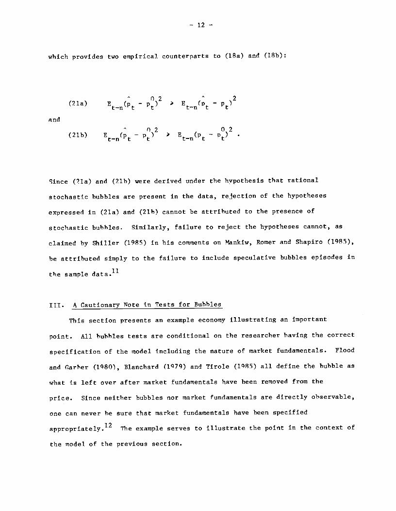
which provides two empirical counterparts to (iRa) and (18b):

(21a) — p)2 E(; — )2

and

1)2 02(21h) — p') ) E_(p —

Since (21a) and (21h) were derived under the hypothesis that rational

stochastic hubbies are present in the data, rejection of the hypotheses

expressed in (21a) and (21h) cannot be attributed to the presence of

stochastic bubbles. Similarly, failure to reject the hypotheses cannot, as

claimed by Shiller (1985) in his comments on Mankiw, Romer and Shapiro (1985),

he attributed simply to the failure to include speculative bubbles episodes in

the sample data.'1

III. A Cautionary Note in Tests for Bubbles

This section presents an example economy Illustrating an important

point. All bubbles tests are conditional on the researcher having the correct

specification of the model including the nature of market fundamentals. Flood

and Garher (1980), Bianchard (1979) and Tirole (1985) all define the bubble as

what is left over after market fundamentals have been removed from the

price. Since neither bubbles nor market fundamentals are directly observable,

one can never be sure that market fundamentals have been specified

appropriately.12 The example serves to illustrate the point in the context of

the model of the previous section.

— 11 —

The Euler equation (1) may be rewritten as

(22) U'(c)z = Et{PIT'(c÷1)(z+1 + a+i)J.

Consider an economy with a+i constant at a and for simplicity assume that

aggregate output is not storable and is constant at y. With population

normalized to one, per capita consumption is simply c = y in equilibrium. We

first solve the model without uncertainty assuming the absence of bubbles.

The solution for price is

(23) z = pa/(l—p), t = 0,1,..'.

Now consider the solution if everyone knows that a government will come into

existence at T. Assume that the government will institute a tax system to

finance its expenditures and that the service flow of government goods enters

the utility function separably from the utility of private goods. Assume also

that the government will take g units of the consumption goods each period,

which lowers equilibrium consumption to c = y — g in each period from T

onwards.

The advent of the government sector raises the marginal utility of

private consumption in period T and thereafter. we parameterize this change

by writing U'(y — g) = (1 + cz)U'(y). Suppose further that the government

finance system taxes all income flows but not capital gains at the rate

so that g = Gy. After—tax income from owning an asset is therefore (l—O)a.

To determine the price of the asset in periods before T, consider first

what price must hold after the advent of the government. The first order

— 14 —

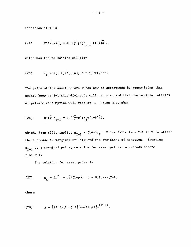
condition at T is

(24) U'(Y—g)z = pu'(y_g)[z1+(l_O)al,

which has the no—hubbies solution

(25) z = p(1—O)a/(1—p), t = T,T+1,•••.

The price of the asset before T can now be determined by recognizing that

agents know at T—1 that dividends will he taxed and that the marginal utility

of private consumption will rise at T. Price must obey

(26) U'(y)z_1 PU'(y_g)(z+(l_O)a),

which, from (25), implies ZT1 = (l)zT Price falls from T—1 to T to offset

the increase in marginal utility and the incidence of taxation. Treating

ZT1 as a terminal price, we solve for asset prices in periods before

time T—l.

The solution for asset price is

(27) z = Apt + pa/(1—p), t =

where

(28) A =

— 15 —

The price path prior to T—1 will rise, fall, or remain constant depending on

the sign of A which is governed by whether (1—O)(1+c&) is greater than, less

than, or equal to one.13

Now supose agents are not sure that a government will be installed at

T. Assume that their uncertainty can he represented by a time—invariant

probability it that the government will begin operation at T with corresponding

probability (1—it) that the government will not begin operation then or any

other time in the future.

With this change the constant term in (28) becomes

(29) A' = 1Tr+(lff)(l+a)(l_O)_lJfpa/(l_pJpT_l

If the transition probability is not constant hut moves through time, a

solution for the price path is

(30) z = Iirt+(1_irt)(1+x)(1_6)_lJfpa/(1_p)JPT_t_l

+ pa/(1—p), t =

which may vary stochastically through time in addition to its deterministic

movements.

The important point about these simple examples is that they illustrate

situations in which an expected future event produces a price path which, if

compared to the path of market fundamentals prior to the future event, appears

to he characterized by a bubble. Examination of (27), (28), (29) and (30)

indicates that asset prices correspond to the no—bubbles with constant

fundamentals price in (23) plus something else. The additional element must

— 16 —

fulfill the bubble property given in equation (4) since it is in the

homogenous part of the solution. The homogenous part will he present in price

either if there are bubbles or if the no bubbles system needs to position

itself in advance of a future switch in forcing processes. The last example

as well as more complex versions would generate stochastic price paths that

would appear to contain stochastic bubbles that satisfy (4) even though the

examples are bubble free.

The econometric problem arises because the Investigator never knows

precisely what information is used by economic agents. Consider a naive

investigator who examined data from periods surrounding the possible

institution of the above government policies in a situation in which the

policies were not instituted. If A' in (29) is nonzero, the unwary researcher

who treated data for at as market funcamentals would conclude that the price

path prior to T contained a bubble that burst. The example, of course, was

bubble free. The problem is that at does not capture all of the market

fundamentals. The potential taxation and government spending programs also

are part of fundamentals.

The point of this section was to provide a cautionary note to the

Interpretation of bubbles research. Empirical bubbles tests must be

Interpreted either conditionally assuming an investigator has correctly

modeled market fundamentals or as joInt tests for bubbles and possibilities of

misspecIfication of market fundamentals. Perhaps the latter interpretation Is

more attractive to some researchers. It Is interesting nevertheless to

inquire whether bubble—type processes characterize the data, and if so, what

misspeciflcation of market fundamentals might he behind such a finding.

— 17 —

IV. ConcludingRemarks

Speculative hubbies are possible in some theoretical models and are

precluded in others. Whether they are important phenomena in actual economic

data is an open question presumably susceptible to scientific investigation.

One point of this paper is that the implementation of variance bounds

tests often precludes rational speculative bubbles as a reason for rejection

of the null hypothesis in such tests. Construction of an observable

counterpart of ex post rational price, Pt, by employing an actual terminal

market price, builds any rational bubbles into the empirical analysis.

Therefore, hubbies must he unrelated to findings that the volatility of Pt IS

greater than that of

Of course, this is not an indictment of variance bounds tests. These

tests play an important role in the econometric analysis of financial

markets. We have observed the controversy surrounding these tests and their

empirical Implementation. Our purpose is simply to clarify these tests and

their empirical implementation on one particular issue.

The second point of the paper is to provide a cautionary note to the

empirical analysis of bubbles. West (1984, 1985) has designed and implemented

theoretically correct hubbies tests. West's methodology requires an

unrejected Euler equation (1) and a forecasting equation for market

fundamentals. Interpretation of the results of such tests requires

consideration of potential changes In the market fundamentals that agents may

he forecasting. Much work has been devoted to attempts to find an unrejected

ruler equation, hut success has been elusive. Less effort has gone into

understanding how process switching can affect asset pricing tests. Both

aspects are critical to our understanding of the economics of asset price

volatility.

— 18 —

Footnotes

The authors thank the National Science Foundation for its support of their

research. They also thank Paul (aplan for helpful discussions.

1. See, in particular, Flavin (1q83), Kleidon (1985a, 19R5h) and Marsh and

Merton (1984).

2. Eichenbaimi and Hansen (1984) and Dunn and Singleton (1985) explore

alternatives that allow considerable variation In the representative

agent's intertemporal marginal rate of substitution.

1. Dornhusch (1952) argues that the flexible exchange rate system has not

worked well and suggests that speculative bubbles may he one of the

culprits. See Meese (1986) for a test of speculative bubbles in the

foreign exchange market.

4. Marsh and Merton (1984) use the sample average price as the terminal price

in constructing their counter example to Shiller's derived variance

hounds.

h5. Satisfaction of a transversality condition such as lim p Et(pt+h) = 0

h+requires the absence of bubbles. Tests for speculative bubbles can

consequently he thought of as tests of this model's transversality

condition.

6. The restrictions that (4) places on the bt process are not very severe.

The time series process can take many possible forms including bubble

innovations that are conditionally heteroscedastic.

7. Tn order to simplify our argument we abstract from the sampling

distribution of the sample statistics and regard them as precise estimates

of their population counterparts.

— 19 —

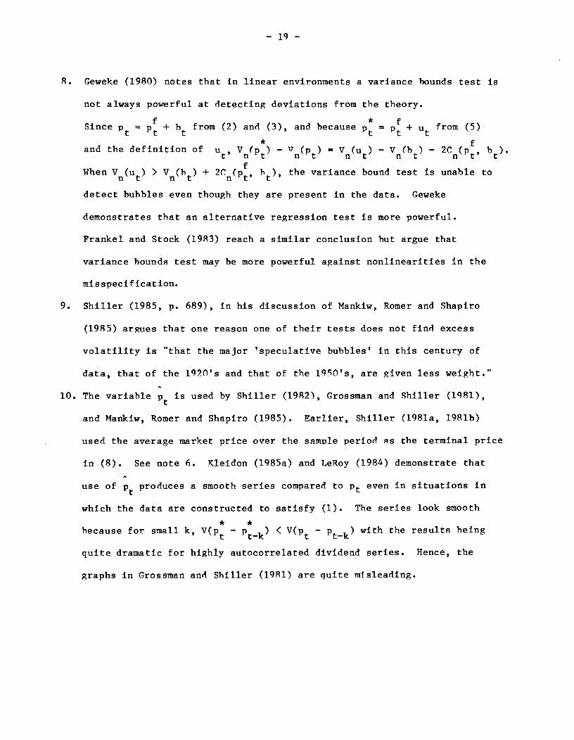
8. Geweke (1980) notes that in linear environments a variance hounds test is

not always powerful at detecting deviations from the theory.

Since Pt = + ht from (2) and (3), and because p = p + u from (5)* f

and the definition ofu, V(Pt) — V(p) = v(u) — v(bt) — 2C(p, he).

When V(u) > V(h) + 2C(p, he), the variance bound test is unable to

detect bubbles even though they are present in the data. Geweke

demonstrates that an alternative regression test is more powerful.

Frankel and Stock (1983) reach a similar conclusion but argue that

variance bounds test may be more powerful against nonlinearities in the

mlsspeciflcat Ion.

9. Shiller (1985, p. 689), in his discussion of Mankiw, Romer and Shapiro

(1985) argues that one reason one of their tests does not find excess

volatility is "that the major 'speculative bubbles' in this century of

data, that of the 1920's and that of the 1950's, are given less weight."

10. The variable Pt is used by Shiller (1982), Grossman and Shiller (1981),

and Mankiw, Romer and Shapiro (1985). Earlier, Shiller (1981a, 1981b)

used the average market price over the sample period as the terminal price

in (8). See note 6. Kleidon (1985a) and LeRoy (1984) demonstrate that

use of Pt produces a smooth series compared to even in situations in

which the data are constructed to satisfy (1). The series look smooth

because for small k, V(p — < V(p — with the results being

quite dramatic for highly autocorrelated dividend series. Hence, the

graphs In Grossman and ShIller (1981) are quite misleading.

— 20 —

11. In fairness to Shiller, his (1984) work clearly indicates that he rejects

the notion of rational speculative bubbles discussed in this paper,

although Fischer (1984) argues that Shiller's fads and fashions may

ultimately prove to he the same thing as speculative bubbles.

12. This point was emphasized by Flood and Garber (1980, pp. 749—50) and has

been reiterated by Hamilton and Whiteman (1985).

13. If U(c) = c' /(1—8), 8 > 0, then (l+)(1—O) = 1 and the type of price

path followed until date T—1 depends on the relationship of 8 to unity.

If 13 > 1, prices rise prior to T while they fall if 8 < 1. For

quadratic utility the relationship of (l+c&)(1—O) to unity will depend on

the scale of the economy and ratios of the utility function parameters.

— 21 —

References

Ackley, 0., 1983, "Commodities and Capital: Prices and Ouantities,"

American Economic Review, March, 1—16.

Blanchard, 0., 1979, "Speculative Bubbles, Crashes, and Rational

Expectations," Economic Letters 3, 387—89.

Blanchard, 0. and M. Watson, 1982, "Bubbles, Rational Expectations and

Financial Markets," in Paul Wachtel (ed.) Crisis in the Economic

and Financial Structure, Lexington Books, Lexington, Ma.

Dornhusch, R., 1982, "EquilibrIum and Disequilibrium Exchange Rates,"

Zeitschift fur Wirtschafts und Sozialwissenshaften 102, No. 6, 573—99.

Dunn, T<. and IC Singleton, 1985, "Modeling the Term Structure of Interest

Rates Under Nonseparable Titility and Durability of Goods,"

Journal of Financial Economics, forthcoming.

Eichenbaum, M. and L. I-lansen, 1984, "Uncertainty, Aggregation, and the

Dynamic Demand for Consumption Goods", Carnegie—Mellon Tiniversity,

manuscript.

Fischer, S., 1984, "Comments and Discussion", Brookings Papers on Economic

Activity 2, 499—504.

Flavin, M., 1983, "Excess Volatility in the Financial Markets:

A Reassessment of the Empirical Evidence," Journal of Political Economy,

December, 929—956.

Flood, R. and P. Garber, 1980, "Market Fundamentals Versus Price Level

Bubbles: The First Tests," Journal of Political Economy, August, 745—770.

— 22 —

Frankel, J. and J. Stock, 1983, "A Relationship Between Regression Tests

and Volatility Tests of Market Efficiency," N.B.E.R. Working Paper

No. 1105.

Geweke, J., 1980, "A Note on Testable Implications of Expectation Models",

University of Wisconsin, Social Science Research Institute.

Grossman, S. and R. Shiller, 1981, "The Determinates of the Variability of

Stock Market Prices," American Economic Review, May, 222—27.

Hamilton, J. and C. Whiteman, 1985, "The Observable Implications of Self—

Fulfilling Expectations." Journal of Monetary Economics 16, November,

353—374.

Hansen, L., 1982, "Large Sample Properties of Generalized Method of Moments

Estimators," Econometrica, July, 1029—54.

Hansen, L. and K. Singleton, 1982, "Generalized Instrumental Variables

Estimation of Nonlinear Rational Expectations Models," Econometrica,

September, 1269—86.

Kleidon, A. 1985a, "Variance Bounds Tests and Stock Price Valuation Models,"

Research Paper 806, Stanford University Business School.

____________________ 1985b, "Bias in Small Sample Tests of Stock Price

Rationality," Paper No. 819, Stanford University Business School.

LeRoy, S., 1984, "Efficiency and Variability of Asset Price," American

Economic Review 74, May, 183—87.

LeRoy, S. and R. Porter, 1081, "The Present—Value Relation: Tests Based on

Implied Variance Bounds", Econometrica, Nay, 555—74.

— 23 —

Mankiw, N. G., 0. Romer and M. Shapiro, 1985, "An Unbiased Reexamination of

Stock Market Volatility," The Journal of Finance, July, 677—89.

Marsh, T. and R. Merton, 1984, "Dividend Variability and Variance Bounds

Tests for Rationality of Stock Market Prices," Unpublished, Sloan School

of Management, Massachusetts Institute of Technology.

Meese, R., 1Q86, "Testing for Bubbles in Exchange Markets: The Case of

Sparkling Rates," Journal of Political Economy, forthcoming.

Scott, L., 1985, "Market Fundamentals Versus Speculative Bubbles: The Case

of Stock Prices in the Tjnited States," University of Illinois, manuscript.

Shiller, R. 1981a, "T)o Stock Prices Move Too Much to he Justified

by Subsequent Changes in Dividends?" American Economic Review,

June, 421—36.

___________________ 1981h, "The TJse of Volatility Measures in Assessing Market

Efficiency," Journal of Finance, June, 291—304.

__________________, 1982, "Consumption, Asset Markets and Macroeconomic

Fluctuations," Carnegie Rochester Conference Series on Public Policy

17, 203—50.

_________________ 1984, "Stock Prices and Social Dynamics," Brookings

Papers on Economic Activity 2, 457—510.

__________________, 1985, "Discussion" The Journal of Finance, July, 688—89.

Singleton, IC, 1980. "Expectations Models of the Term Structure and

Implied Variance Bounds," Journal of Political Economy,

December, 1159—76.

Tirole, J., 1985, "Asset Bubbles and Overlapping Generations,"

Econometrica 53, November, 1499—1528.

— 24 —

West, K., 1984, "Speculative Bubbles and Stock Price Volatility,"

Princeton University, Financial Research Memorandum No. 54,

December.

__________________ 1985, "A Specification Test for Speculative Bubbles",

Princeton University Financial Research Center Memorandum No. 58.