NBER WORKING PAPER SERIES

ANTICIPATIOr'IS, RECESSIONS AND POLICY:AN INTERTEMPORAL DISEQUILIBRIUM MODEL

Olivier J. Blanchard

Jeffrey Sachs

Working Paper No. 971

NATIONAL BUREAIJ OF ECONOMIC RESEARCR1050 Massachusetts Avenue

Cambridge MA 02138

August 1982

This paper was prepared for the Conference on "InternationalAspects of Macroeconomics in France," in Fontainehleau, July 1982.We thank Data Resources, Inc., for letting us use their computer,and the National Science Foundation for financial assistance.The research reported here is part of the NBER 's research programin Economic Fluctuations. Any opinions expressed are those of theauthors and not those of the National Bureau of Economic Research.

NBER Working Paper #971August 1982

Anticipations, Recessions and Policy:An Intertemporal Disequilibrium Model

ABSTRACT

This paper presents an intertemporal disequilibrium model with rational

expectations, i.e. a model in which agents anticipate the future rationally,

but in which prices and wages may not adjust fast enough to maintain contin-

uous market clearing. Therefore, optimizing firms and households base their

intertemporal plans on anticipations of both future quantity constraints and

future prices.

Such a model shows clearly that the effect of a policy depends not only

on its current values but its anticipated path. After a presentation of

the model and its basic dynamics, we therefore consider the effects of

various paths of fiscal policy on the economy.

Olivier J. BlanchardDepartment of EconomicsHarvard UniversityCambridge, MA 02138(617) 495—2119

Jeffrey SachsDepartment of EconomicsHarvard UniversityCambridge, MA 02138(617) 495—4112

Introduction

Both France and the United States have recently experienced major

political changes. As a result, current economic policy is different from

what it was, and even larger changes are anticipated in the coming years.

Although the goal of those policies is to accomplish structural changes,

stronger defense and less government intervention in the U.S. , more equal

income distribution and industrial reorganization in France, they will have

and already are having macroeconomic effects on investment, consumption and

employment. High anticipated deficits are blamed for the high long-term

real interest rates in the U.S., anticipations of a higher fiscal burden

on firms are blamed for the sluggishness of private investment in France.

The purpose of this paper is to present a model in which effects of

anticipated as well as current changes in policy can be analyzed. Techni-

cally the model is an intertemporal disequilibrium model with rational

expectations, i.e. a model in which agents take the anticipated future

into consideration as rationally as they can, but where prices and wages

may not adjust fast enough to maintain full employment. The paper therefore

builds on two recent strands of research in macroeconomic fluctuations:

rational intertemporal choice and disequilibrium analysis.

The first approach has emphasized that most decisions are intertemporal

and thus depend as much on anticipated as on current prices. It has focused

in particular on intertemporal substitution of consumption or leisure by

households, on the optimal employment-investment decisions by firms (see

for example, books by Barro [31, Lucas [18], Sargent [24]). This approach

has led to a better understanding of the dynamic effects of either policies

or real disturbanc's (in oui own work for example, fiscal policy [2], oil

2

price shocks [221). Almost all of the work in this area has, however,

maintained the assumption of market clearing, at least in the goods market

(Hall [121 and Sachs [221 allow for a nonlabor market clearing real wage)

The second approach, disequilibrium theory, has emphasized that, if

prices are not fully flexible, most decisions must take into account not

only prices but quantity constraints. It has focused in particular on the

implications for consumption and labor supply decisions by households, and

for employment decisions of firms, giving a better foundation to many

standard macroeconomic relations. It has shown how equilibria correspond

to different regimes, each with distinct implications for policy. Although

most of the work in this area has recognized the potential importance of

anticipated future constraints (most notably Malinvaud [201), it has usually

not modeled behavior explicitly as intertemporal or considered the implica-

tions of rational expectations (an exception is Neary and Stiglitz [211).

Can both approaches be combined? We believe that they can, in that

agents attempt to make rational choices and to anticipate the future, even

when some prices are not fully flexible. We realize that the assumption of

rational expectations is overly strong and the lack of explicit foundations

of price inertia is unsettling. Rational expectations appear however to be

the most neutral way of allowing agents' decisions to depend on the future.

We also believe that a model with more firmly grounded price inertia

(possibly from desynchronization, such as in [25] and [8]) would lead to

similar results, although we have not in this model attempted such an

undertaking.(1)

The model we derive is slightly beyond analytical tractability. An

analytical treatment can only be offered by taking shortcuts, something

3

we have explored in [6], [9]. The choice here has been to solve the

complete model by numerical simulations. Given that the model is derived

from maximizing behavior and that its size is small enough, results can

easily be traced to specific assumptions about parameters and policy.

The paper is organized as follows: Section I characterizes households'

and firms' behavior, as well as the intertemporal equilibrium. In

particular, it clarifies the role of short and long interest rates in

investment and consumption decisions, and the relation between market value,

profit, profitability, the real wage and investment. It shows how the

expectation of future constraints may lead to anticipatory buying by

consumers and firms. Section II displays the basic dynamic mechanisms of

the model, through a focus on the following questions: What is the role

of investment, both through demand and supply, in the transmission of

shocks, a question stressed by Malinvaud [20]? Can sharp deflations in

response to lower money growth be destabilizing, as suggested by Keynes

and more recently by Tobin [26]? Is the responsiveness of real wages to

unemployment stabilizing or destabilizing, a question raised throughout

the research on disequilibrium (starting with Barro—Grossman [4])?

Section III returns to one of the policy issues relevant in France today:

What happens if firms anticipate an increase in their fiscal burden in the

future? No attempt is made to fit specific facts and magnitudes, our

intention being to clarify the various economic forces set in play by such

anticipations. More generally, our focus in most of the paper is as much

on methodology as on substantive economic issues. Carefully calibrated

simulation models will be necessary to reach firm answers to many of the

issues raised in the paper.

4

Section I. The Model

General description

Our choice has been to build the simplest model in which households

and firms have nontrivial intertemporal choices. Thus, we assume that the

economy is closed and that there is one produced good, used either for

consumption or investment. There are three tradable assets, money, debt

and equities.

Households and firms take as given both current and anticipated prices

and quantity constraints. Although the future may be uncertain, they act

as if they know it with certainty.(2) Households are all identical and

maximize the discounted sum of utility; their problem is intertemporal as

they have to choose between consumption now or consumption later. Firms

are identical and maximize their value, which is the discounted sum of

anticipated cash flows. Labor is a variable factor but capital is quasi-

fixed: changes in capital are costly, so that the investment decision

presents also an intertemporal problem.

The solutions to the maximization problems of households and firms

give a set of actual demands (or supplies) which satisfy both the budget

constraint and (current and anticipated) quantity constraints. (These are,

in the disequilibrium terminology, Drèze" demands [11]). We can also, for

both maximization problems, find for each constraint the lowest value of

this constraint such that it is not binding. We shall refer to this set

of values as the set of shadow demands (these correspond to "Benassy"

demands). It follows that each actual demand can be expressed as the

minimum of the constraint and the shadow demand.

5

Each market has rationing rules governing the allocation of goods to

the constrained side; we allow these rules to depend on shadow demands.

Market clearing requires that two conditions be satisfied: the first is

that at most one side of the market be constrained, the second that actual

demand and actual supply be equal. We follow others in this field by

allowing asset prices to adjust and thus asset markets to clear. We do

not however follow standard usage in our treatment of the labor market:

we assume that households supply all the labor demanded by firms and that

firms are therefore never constrained in the labor market. By doing so,

we eliminate the regime of urepressed inflationu (following Malinvaud's

terminology {19]) and are left with only two regimes, a "Keynesian regimefl

when suppliers of goods are constrained and a "classical regime" when

buyers of goods are constrained. We feel that little is lost by this

simplification, at least for the experiments we consider, and that the

benefit in increased simplicity is substantial.

Prices adjust over time as functions, not of excess actual demands

which are, by construction, identically zero, but of excess shadow demands.

At any time t, an intertemporal equilibrium is a sequence of shadow

demands, a sequence of actual demands and a sequence of prices, consistent

with maximizing behavior and the rationing rules, such that both current

and future markets are anticipated to clear. If exogenous variables take

over time their anticipated values, the intertemporal equilibrium is

actually realized over time. If at some time t+T, there are unanticipated

changes in current or anticipated exogenous variables, a new intertemporal

equilibrium for period t+t and future periods must be recomputed.

We now describe the model in detail.

6

The behavior of firms

All firms are identical and we shall not distinguish between individual

and aggregate values. The time index t will also be deleted, whenever

convenient.

The technology of the firm is characterized by:

A production function, with constant returns to scale:

Q = F(K, L)

An installation function, giving the number of goods used up in installation

of I units of investment:(3)

Ic(I/K) ; t() >

The total number of goods needed to invest at rate I is therefore:

J=I+Iq(I/K) = 1(1+ (I/K))

An accumulation equation, with exponential depreciation at rate p:

= I -

The firm takes as given the sequence of real wages and real interest

rates {w/p, r}0 and the sequence of constraints on the amount of

goods it can sell and the amount of goods it can invest, ' I}..=o.

By assumption, there are no constraints on the amount of labor it can buy.

The firm maximizes its value, which is the present value of cash flows:

t—Jrds

v=j (Q-(W/P)L-J)e Os dt0

7

t—f r dsC S

Let e be the costate variable associated with the accuntulation

equation, and XQI the Lagrangians associated with the quantity

constraints; the Hamiltonian is therefore:

t—frdsH = e 0 S

[F(K, L) — (W/P)L - 1(1 + 4(1/K)) + q(I -

+ XQ(Q — F(K, L)) + A1(I — I)]

Necessary conditions for maximization are:

FL(K1 L) (1 -XQ)

= w/P ; XQ(Q — Q) = 0 ; AQ > 0

1 + (I/K)4'(I/K) + 4(1/K) = q—X1 ; A1(I—I) = 0 ; > 0

= (r + p)q - (1 -XQ)FK(Kl

L) - (I/K)24' (I/K)

—f r dsOslimet-*cc

They can be rewritten more intuitively as follows:

Define shadow labor demand and quantity supply Ld, Q5 s.t.:

(1) Ld, Q5IF(Ld K) = W/P QS = F(K, Ld)

(2) Then 9 = min(Q5, 9) ; LF(K, L) = 9

Define shadow investment and investment spending, 1d, d s.t.:

(3) 1d d1 + 4(Id/K) + (Id/K)4, (Id/K) = q ; d = 1d(1 + 4(Id/K))

(4) Then I = min(Id, I) ; 3 = min(J', J) , 3 E 1(1 + c(I/K)) and:

8

(5) q = (r±)q (W/P)(FK(K, L)/FL(K, L)) - (I/K)2'(I/K)r ds

(6) urn e = 0

Given the capital stock, the real wage and the possibly binding output

constraint, the employment and output decisions of the firm are straight-

forward. The investment decision is of more interest and is characterized

by equations 3 through 6: To see what they imply, we can rewrite them

further. Inverting (3), and integrating (5) forward subject to the

transversality condition (6) gives:

(7) I = min(Id, I) ; Id/K = H(q) ; H(l) = 0 ; H'(.) > 0

!t(r +.ti(8) q =

J ((w/P)(FK(K, L)/FL(K, L)) (I/K)2(I/K)Je

Investment is the minimum of shadow investment and the constraint.

Shadow investment in turn depends on q, the present value of marginal

profits, usually called Tobin's q. Marginal profit is the sum of two

terms; the second is the reduction in the cost of installation made possible

by an additional unit of capital and is a minor factor in profits. The

first is more interesting and depends very much on the regime.

In the classical regime, i.e. if the firm is not output constrained,

the marginal product of labor equals the wage and this first term is simply

the marginal product of capital. Furthermore, if the firm does not

anticipate to be ever output constrained in the future, a particularly

nice result arises: the shadow price q is equal to the observable average

value of capital V/K (Hayashi [13]). In the absence of constraints on

investment spending, there is then a direct relation between the firm's

9

value and its investment behavior. An increase in the real wage for example

decreases employment, the marginal product of capital, and thus investment

and the value of the firm.

In the Keynesian regime, the firm is output constrained. The first

term then is the marginal wage savings, i.e. the real wage times the

marginal rate of substitution. There is no longer a close relation between

q and V/K, between investment and the value of the firm. The effect of an

increase in the real wage is now to increase the marginal wage savings and

to increase q and investment as capital becomes more attractive than labor

to produce the same level of output. Although it now increases investment,

the increase in the wage still decreases profit and thus the value of the

firm. An increase in output increases both marginal and average profit and

thus both q and V/K. (4)The effect on marginal profit however depends on

the elasticity of substitution5 while the effect on average profit does

not.

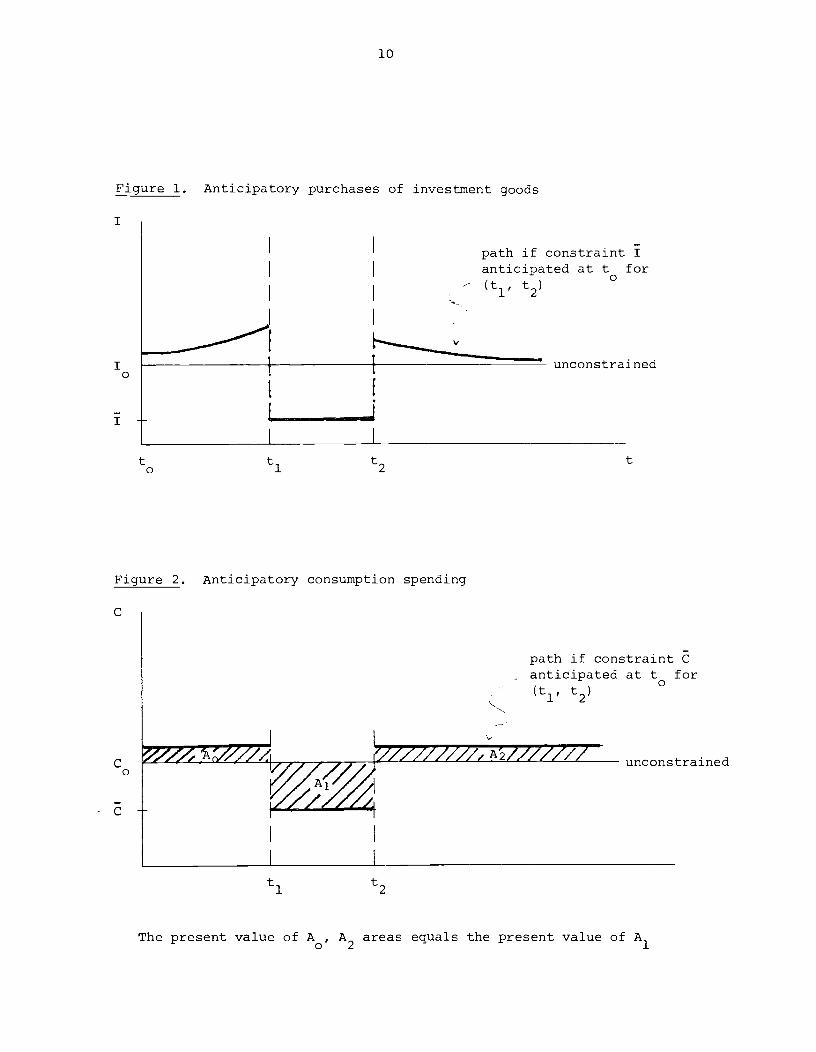
Finally, the effects of a constraint on investment demand are easily

characterized. Anticipated constraints on investment demand lead, ceteris

paribus, to an anticipated lower capital accumulation, thus to higher

marginal profits, to a higher q and higher investment demand today. It

therefore generates anticipatory buying of investment goods. The effect

is represented graphically in Figure 1.

Since asset markets are assumed to clear and the financial structure

of firms is thus irrelevant for firms' or agents' decisions, the following

structure is convenient: Firms have real debt B outstanding, paying the

real interest rate. They finance all investment from retained earnings

and do not issue new debt or new equity. The assumption that there is

10

Figure 1. Anticipatory purchases of investment goods

path if constraint Ianticipated at to for

— (t1, t2)

unconstrained

The present value of A, A2 areas equals the present value of A1

I

I0

I -jt0 ti t2

Anticipatory consumption spending

t

Figure 2.

C

C0

C

path if constraint Canticipated at to for

(t1, t2)

unconstrained

tl t2

11

real debt outstanding implies that there is an observable interest rate but

is otherwise irrelevant. (The assumption that all investment is internally

financed implies that in equilibrium personal savings are zero.) The amount

of profits paid to equity owners is as a result:

(9) 7t(Q-(W/P)L—J-rB)

The behavior of consumers—workers

All consumers are identical and we shall not distinguish between

individual and aggregate values.

Consumers derive utility from consumption and real money balances.

Leisure does not explicitly enter the utility function; desired labor supply

is L*. Households take as given the sequence of prices, real wages, real

interest rates and profits paid to equity owners, as well as the sequence

of labor they supply and the amount of goods they can buy

They maximize the present value of utility:

= u(C, M/P)et dt

Defining A E B + M/P, the budget constraint can be written as:

A = rA + (W/P)L + ir — ((r +/P)(M/P) — c)

Define the costate variable associated with the budget constraint as e5tx,

and the Lagrangian associated with the quantity constraint on consumption

as X. The Hamiltonian is then:

H = et[u(c, M/P) + X(C_C) + x(rA + (W/P)L + - (r+P/P)M/P —

12

Necessary conditions for maximization are:

u(C, M/P) = x + ; Xc(C— C) 0 ;

XC> 0

Um(C1 M/P) = x(r+P/P)

x = (—r)x

—turn e x = 0t-*

They can be rewritten more intuitively as follows:

Define shadow consumption demand Cd such that:

(10) CdIUC(Cd, M/P) = x

(11) Then C = rnin(Cd, C)

(12) Um(Ci M/P) = x(r+P/P)

—St(13) x = (—r)x ; Urn e x = 0

t+

In the absence of constraints on consumption, consumers equalize the

marginal rate of substitution between money balances and consumption to the

nominal interest rate. The path of consumption is determined by (13) which

gives the behavior of marginal utility,and the budget constraint. Approxi-

mately, (13) gives the shape of the path and the budget constraint the

highest feasible level of this path.

Current constraints on consumption lead to forced savings and more

consumption later. Anticipated constraints have the same effect on

consumptin as on investment. They lead to anticipated forced savings,

13

thus to a higher feasible level of consumption today. The effect is

represented graphically in Figure 2 when 5 = r and M/P is constant, so

that agents choose the highest feasible constant level of consumption.

We shall introduce the government later.

Equilibrium given prices and wages

Equilibrium in the goods market requires that actual supply equals

actual demand. It also requires that at most one side be constrained.

From (2), actual aggregate supply is

5 —

Q = min(Q , Q)

From (4) and (11), actual aggregate demand is

Q=min(Qd,Q) where Qd=cd+Jd

The above conditions for equilibrium imply:

(14) Q = min(QS, Qd)

Rationing rules are as follows: If supply is constrained, there is

uniform rationing of firms. If demand is constrained, consumption and

investment are rationed according to:

(15) C = - a(Qd — Q) ; a [0, 1]

l6) = d - (l_a)(Qd_Q) ; 111(1 + (I/K)) = jThus, in general, rationing depends on shadow aggregate demand. If a

equals 0 or 1, however, there is rationing of investment only or

consumption only.

14

In the labor market, we have assumed that firms can always hire the

labor they demand. Thus, labor is given by:

(17) LjF(L, K) = Q

Movement of 2rices and wages

Although there is by construction zero excess actual demand in all

markets, shadow excess demands may be different from zero. Thus a natural

assumption is to allow prices and wages to respond to these excess demands

(6)over time. They are assumed to follow:

(18) = (Qd - QS)

(19) W/w = 8(L — L*) + aP/P

B, 8 measure the response of prices and wages to goods and labor market

conditions. a measures the degree of indexing of wages.

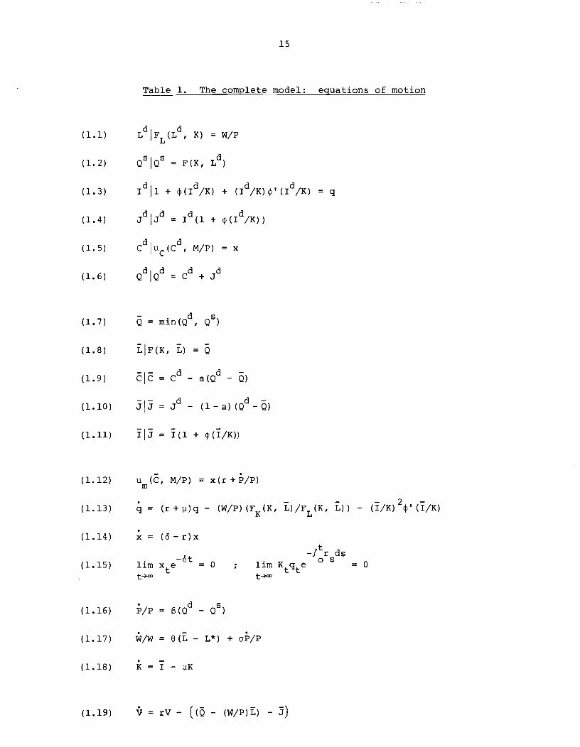
Intertemporal equilibrium

The set of equations is reorganized and presented in Table 1. Equations

(1.1) to (1.6) give shadow demands and supplies. These depend on three sets

of variables, policy variables (M) , state variables given from the past

(P, w, K) and costate variables which depend on the anticipated future (q, x).

Equations (1.7) to (1.11) show how actual demands and supplies follow from

shadow demands and supplies.

Equation (1.12) determines the real interest rate from equality of

money demand and money supply. Equations (1.13) and (1.14) give the

equations of motion of the costate variables (q, x), equations (1.16) to

(1.18) the equations of motion cf the state variables (P, W, K). Finally,

(1.1)

(1.2)

(1.3)

(1.4)

(1.5)

(1.6)

(1.12)

(1.13)

(1.14)

(1.15)

(1.16)

(1.17)

(1.18)

15

Table 1. The complete model: equations of motion

LdFL(Ld, K) = w/P

Q51Q5 = F(K, Ld)

1d1 + q(Id/K)

= 1d(1 +

CuC(Cd, M/P)

QdQd = +

(Qd - QS)

e(L - L*) + oP/P

- ilK

(1.19) V = rV — ((Q — (W/P)L) —

+ (Id/K)t (Id/K) = q

(Id/K))

=x

(1.7)

(1.8)

(1.9)

(1.10)

(1.11)

= min(Qd QS)

LIF(K, L) = Q

= — a(Qd — Q)

= d - (l_a)(Qd_Q)

IJ = 1(1 + HI/K))

U(C, M/P) = x(r+P/P)

q = (r+)q -(W/P)(FK(K, L)/FL(K, L)) - (I/K)2'(I/K)

x = (6—r)x

—1Stl1mxe =0t-*o

=

=

i

t—f r dsOs

urn =0

16

equation (1.19) gives the behavior of V, which does not affect any other

variable in the model.

At any point of time, an intertemporal equilibrium is a sequence of

quantities (Ld, QS 1d d cd, Qd L, Q, I, J, C, K) and a sequence of

prices (r, q, x, P, W, V) which, given the sequence of policy (M) and

initial conditions (?, W, K) satisfy equations (1.1) to (1.19) for the

current and all future periods.

Steady state

Before we turn to the dynamics, we briefly characterize the steady

state of the model, when P = W = K = x = q = 0. We denote steady state

values by stars. Intertemporal utility maximization implies, from (1.14)

that r* = 6. The interest rate is always equal to the subjective discount

rate in steady state; equivalently the long—run elasticity of savings at 6

is infinite. From (1.3) and (1.18), as I = 1d, q must be sufficient to

generate gross investment equal to depreciation:

q* = 1 + (i-') + iiq:'(p) > 1

In turn, (1.13) determines the marginal product of capital and thus the

steady state level of capital stock:

K*IFK(K*, L*) + p2'() = (6+p)q*

If p = 0, so that q = 1, this condition reduces to the familiar condition:

L*) = (6+p)

17

Consumption is determined by:

C = F(K*, L*) — UK*(1 + (p))

Finally, the level of real money balances is given by:

Um(C* M/P*)/uc(C*I M/P*) =

Money is clearly neutral in the long run in this model.

Section II. Comparative Dynamics

To show the basic dynamics of the model, this section concentrates on

the dual role of investment as a determinant of demand and later of supply

through capital accumulation, and on the stabilizing or destabilizing role

of prices and wages.

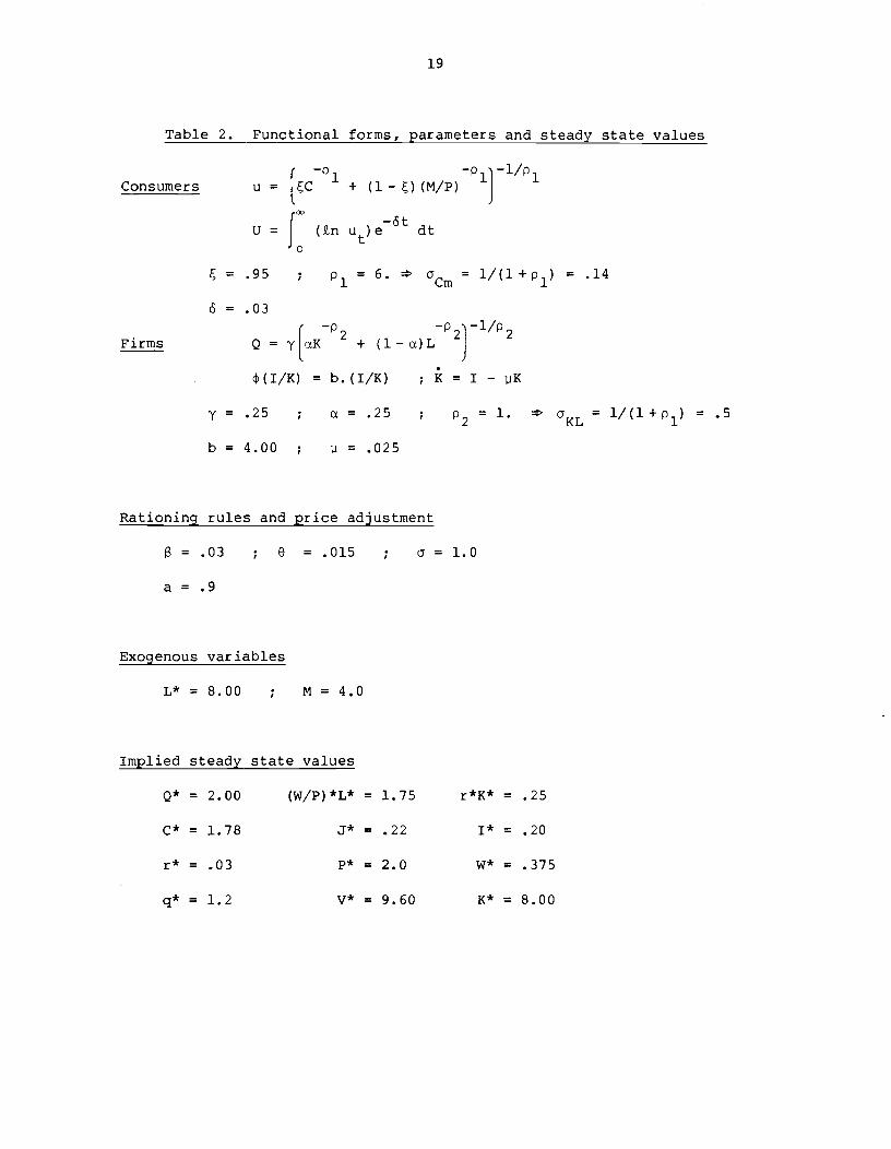
Functional forms and parametrization

To simulate the model, specific functional forms must be chosen for

utility and technology,and numerical values must be chosen for the

parameters. These assumptions are summarized in Table 2.

Instantaneous utility is CES in consumption and money balances. The

elasticity of substitution between utility in different periods is assumed

to be unity, so that cardinal utility is logarithmic. (Under uncertainty,

this last assumption implies unit constant relative risk aversion.)

- The production function is also CES in capital and labor. The

installation function 4(I/K) is linear in I/K, so that total cost of

installation is quadratic in I.

18

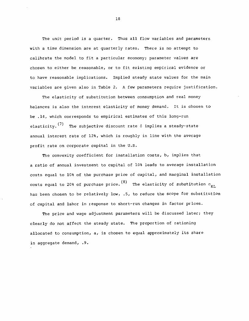
The unit period is a quarter. Thus all flow variables and parameters

with a time dimension are at quarterly rates. There is no attempt to

calibrate the model to fit a particular economy; parameter values are

chosen to either be reasonable, or to fit existing empirical evidence or

to have reasonable implications. Implied steady state values for the main

variables are given also in Table 2. A few parameters require justification.

The elasticity of substitution between consumption and real money

balances is also the interest elasticity of money demand. It is chosen to

be .14, which corresponds to empirical estimates of this long—run

elasticity.(7) The subjective discount rate 5 implies a steady—state

annual interest rate of 12%, which is roughly in line with the average

profit rate on corporate capital in the U.S.

The convexity coefficient for installation costs, b, implies that

a ratio of annual investment to capital of 10% leads to average installation

costs equal to 10% of the purchase price of capital, and marginal installation

costs equal to 20% of purchase price.(8) The elasticity of substitution °KL

has been chosen to be relatively low, .5, to reduce the scope for substitution

of capital and labor in response to short-run changes in factor prices.

The price and wage adjustment parameters will be discussed later; they

clearly do not affect the steady state. The proportion of rationing

allocated to consumption, a, is chosen to equal approximately its share

in aggregate demand, .9.

19

Table 2. Functional forms, parameters and steady state values

Consumers—p1 —p1 —i/p1

u = C + (1—)(M/P)

U = (th ut)et dt

= .95 ; p1= 6. GCm = l/(l+p1) = .14

= .03

p2 —p2 —1/p2Q = y aX + (1-a)L

(I/K) = b.(I/K) ;K = I —

y = .25 ; a = .25 ; p2= 1. °KL = l/(l+p1) = .5

b = 4.00 ; p = .025

Rationing rules and

0

a = .9

price adjustment

.015 ; a=1.0

Exogenous variables

L* = 8.00 ; M = 4.0

steady state values

= 2.00 (W/P)*L* = 1.75

= 1.78 = .22

= .03 = 2.0

q* = 1.2 v* = 9.60

r*K* = .25

1* = .20

= .375

= 8.00

Firms

Implied

r*

20

Method of solution

Dynamic simulations present two problems usually not encountered in

macroeconomic simulations:

The first is standard in rational expectations models. The initial

values of q, x and V are not given from the past but determined from the

requirement that the transversality conditions be satisfied. A dynamic

simulation is thus a two—point boundary value problem, with initial

conditions K, P, W and terminal conditions for q, x and V, (i.e. the

transversality conditions). The technical method of solution is that of

multiple shooting (see 1161 for details)

The second is specific to disequilibrium models and comes from the

presence of minimum functions. We replace the minimum function ((1.7) in

Table 1) by a CES function with low elasticity. In practice, an elasticity

of .005 is enough to replicate the minimum rule.

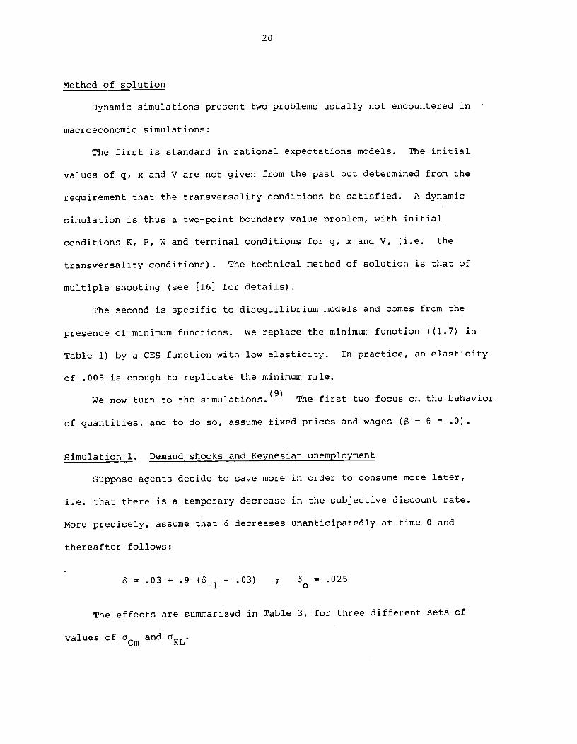
We now turn to the simulations.9 The first two focus on the behavior

of quantities, and to do so, assume fixed prices and wages ( = B = .0)

Simulation 1. Demand shocks and Keynesian unemployment

Suppose agents decide to save more in order to consume more later,

i.e. that there is a temporary decrease in the subjective discount rate.

More precisely, assume that decreases unanticipatedly at time 0 and

thereafter follows:

= .03 + .9 — .03) ; 5 = .025

The effects are summarized in Table 3, for three different sets of

values of a and aCm KL

21

Table 3. A temporary decrease in the discount rate; P, w fixed

High cc

(Flat LM)

(a 2.;a =.5)Cm KL

All variables are in % deviation from steady state except

u : unemployment rate, measured in %

r : absolute deviation from steady state, measured

Low °KL

(Steep IS)

(a = 2.; = .1)Cm

in % at annual rate

Reference case

(a = .14; a = .5)Cm KL

Quarter:

Variable

C

q

QD

QS

r

V/K

u

1 2 3 4 5 6 7 8 9

0 4 12 0 4 12 0 4 12

—2.6 —1.6 — .7 —6.8 —4.3 —1.0 —2.5 —1.6 — .7

1.0 .2 — .1 —3.3 — .7 .5 —3.0 .4 .2

—1.9 —1.6 —1.0 —8.7 —4.8 —1.5 —4.7 —1.4 — .6

.0 .3 .3 .0 — .8 — .7 .0 — .8 — .3

—2.0 —1.2 — .4 — .4 — .4 — .0 —2.0 —1.2 — .8

3.6 2.2 .7 2.3 2.0 1.6 3.5 2.3 1.1

2.0 1.7 .9 11.0 5.5 1.2 5.4 1.4 .5

22

The central role is played by investment. Lower aggregate demand

lowers output and this in turn has two effects: it lowers the demand for

money and thus the sequence of anticipated interest rates; it lowers the

sequence of anticipated marginal profits. Which of the two lower sequences

dominates and whether q and investment go up or down depends crucially on

0Cm and If is large, the demand for money is very interest

elastic, interest rates decrease little and q goes down. If is very

small, the decrease in output and employment reduces strongly marginal

(10)profit and q also goes down. These two cases are shown in columns 4

to 6 and 7 to 9 respectively.

The response of investment in turn, through a multiplier effect,

decreases consumption. The larger and more prolonged the decrease in

investment, the larger the initial decline in consumption and thus the

overall recession. The similarity of our results to the simple ISLM is

striking: the impact effect is larger, the flatter the 114 (the larger

the steeper the IS (the smaller GKL). As the recession slowly

ends, net investment becomes positive again. In none of the three cases

does the economy experience a supply constraint; it always remains in

Keynesian unemployment.

Table 3 also shows clearly the different behavior of marginal q which

affects investment and is unobservable, and average q which might be

observable through the stock market valuation of firms. Although q may

go down, V/K goes up in all three cases: the effect of lower real rates

dominates the effect of lower average profit. Thus, the stock market goes

up while output and possibly investment go down.

23

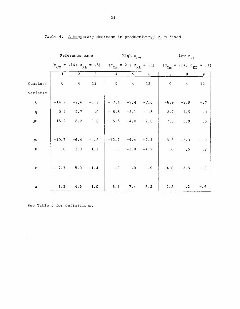
Simulation 2. Supply shocks and classical unemployment

Suppose that the economy is affected by an adverse, unanticipated

technological shock which disappears over time. More precisely, assume

that - follows after t0

(y — .25) = .9 (y — .25) = .2375

This decrease of productivity of 5% initially is in the spirit of a

temporary increase of the price of oil (see [221 for a specific treatment

of such an increase with a more adequate treatment of technology). The

effects are summarized in Table 4, again for three sets of values of

and cKL.

The central role is again played by investment, this time not as a

component of demand but as a determinant of supply through capital

accumulation. The impact effect on production however depends only on

the technology: after the decrease in productivity, employment must

decrease until the marginal product of labor is again equal to the

unchanged real wage. The size of the adjustment depends on °KL If

is low, the required decrease in employment is small; if cYKL is larger,

the decrease is larger. The impact effect on the marginal product is

independent of aKL to the first order and proportional to the share of

capital in output.

The adjustment process and the length of the period of classical

unemployment depends however very much on investment. Two effects are

again present: the first is a lower sequence of real interest rates, the

second is a lower sequence of marginal products. Whether the first or the

second domir.ates depends again on the interest elasticity of money demand.

Quarter:

Variable

C

q

QD

QS

K

r

24

Table 4. A temporary decrease in productivity; P, W fixed

See Table 3 for definitions.

Low a

Cm = .14;

Reference case

(a .14; a = .5)Cm KL

High °Cm

cm = 2.; GKL .5)

KL

aRL = .1)

1 2 3 4 5 6 7 8 9

0 4 12 0 4 12 0 4 12

—14.2 —7.6 —1.7 — 7.4 —7.4 —7.0 —6.9 —3.9 —.7

5.9 2.7 .0 — 5.5 —3.1 — .5 2.7 1.5 .0

15.2 8.2 1.6 — 5.5 —4.0 —2.0 7,6 3.9 .5

—10.7 —6.4 — .2 —10.7 —9.4 —7.4 —5.8 —3.3 —.9

.0 1.0 1.1 .0 —2.8 —4.9 .0 .5 .7

— 7.7 —5.0 —1.4 .0 .0 .0 —4.6 —2.8 —.5

8.2 4.5 1.0 8.1 7.4 6.2 1.3 .2 —.6U

25

Columns 4 to 6 show howif interest rates do not adjust, investment falls

and the recession is substantially deeper and longer.

What happens to shadow aggregate demand in the process of adjustment

is ambiguous. Although both q and wealth may go down, the anticipation of

constraints on both consumption and investment spending may lead both

consumers and firms to attempt anticipatory buying. The anticipatory

buying effect dominates in the first and third cases in Table 4, the lower

wealth and q effect dominates in the second case. In all cases, however,

shadow aggregate demand is less than supply and both firms and consumers

are rationed in their purchases. Thus investment is less than the value

implied by q.

We now turn to the effects of price—wage dynamics on the process of

adjustment. For this, we shall consider the effects of an unanticipated

decrease in nominal money by 5% which is assumed by agents to be permanent.

The reference values of , a, 0 are .03, 1., .015 respectively. The value

of implies that an excess shadow demand of 10% increases prices by 2.4%

over a period of a year. The value of a implies complete indexing of

wages and the value of 0 implies that 5% unemployment in excess of the

natural rate (zero in our model) decreases real wages by 2.4% over a

period of a year.

Simulation 3. The adjustment of prices and the stabilizing Mundell effect

Tobin [261 recently formalized an argument of Keynes that a fast

adjustment of prices may lead to a larger recession in response to a

decrease in money growth: If prices adjust fast, there will be a large

decrease in inflation and expected inflation. Thus real rates will

26

increase both because of higher nominal rates and because of lower expected

inflation; this second channel is usually referred to as the Mundell effect.

Thus the faster the prices adjust, the larger the Mundell effect, the higher

the real rate and the larger, Tobin suggests, the effect on aggregate

(12)demand.

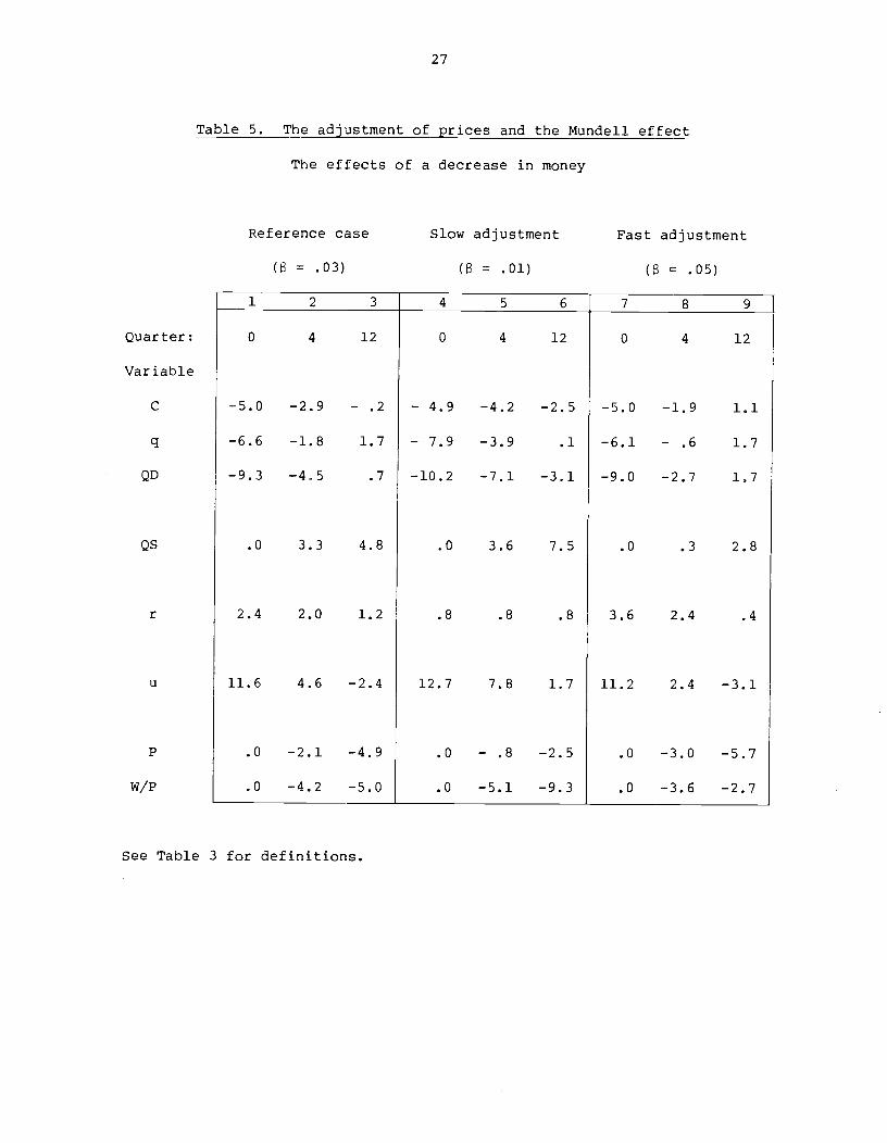
We now check in our model the effects of the speed of adjustment of

prices on the impact of the decrease in money and the length of the

recession. The results are given in Table 5 for three values of , .01,

.03, .05.

The Mundell effect is present: the faster the adjustment of prices,

the larger the increase in the initial interest rate. The impact effect

of the decrease in money is however smaller, the faster prices adjust.

The reason for both results in this model is clear: faster price adjustment

indeed means higher real rates initially, but lower nominal and real rates

later as real money balances increase faster; the faster the price adjustment,

the lower the increase in long real rates. Consumption, through wealth, and

investment, through q,depend mostly on long real rates. The short—term rate

has only one direct effect, given wealth and q, the effect of bending the

path of consumption (equation (1.14)) and to induce consumers to postpone

consumption temporarily. The simulations suggest that this effect, although

present, is not very strong. Thus, in our model, faster price adjustment

leads to a smaller and shorter recession, contrary to Tobin's analysis.3)

Note that the long period of high unemployment leads to lower real

wages. In all three cases, these lower real wages require a period of

overemployment: after the initial recession, the economy experiences a

temporary boom, starting in quarte. 8 in the first case, in quarter 16 in

27

Table 5. The adjustment of prices and the Mundell effect

The effects of a decrease in money

Reference case Slow adjustment Fast adjustment

= .03) ( = .01) ( = .05)

1 2 3 4 5 6 7 8 9

Quarter: 0 4 12 0 4 12 0 4 12

Variable

C —5.0 —2.9 — .2 — 4.9 —4.2 —2.5 —5.0 —1.9 1.1

q —6.6 —1.8 1.7 — 7.9 —3.9 .1 —6.1 — .6 1.7

QD —9.3 —4.5 .7 —10.2 —7.1 —3.1 —9.0 —2.7 1.7

QS .0 3.3 4.8 .0 3.6 7.5 .0 .3 2.8

r 2.4 2.0 1.2 .8 .8 .8 3.6 2.4 .4

u 11.6 4.6 —2.4 12.7 7.8 1.7 11.2 2.4 —3.1

P .0 —2.1 —4.9 .0 — .8 —2.5 .0 —3.0 —5.7

w/P .0 —4.2 —5.0 .0 —5.1 —9.3 .0 —3.6 —2.7

See Table 3 for definitions.

28

the second, and quarter 6 in the third. The boom is a Keynesian boom, with

aggregate demand below supply. The economy thereafter returns to equilibrium.

We now turn to the effects of the speed of real wage adjustment.

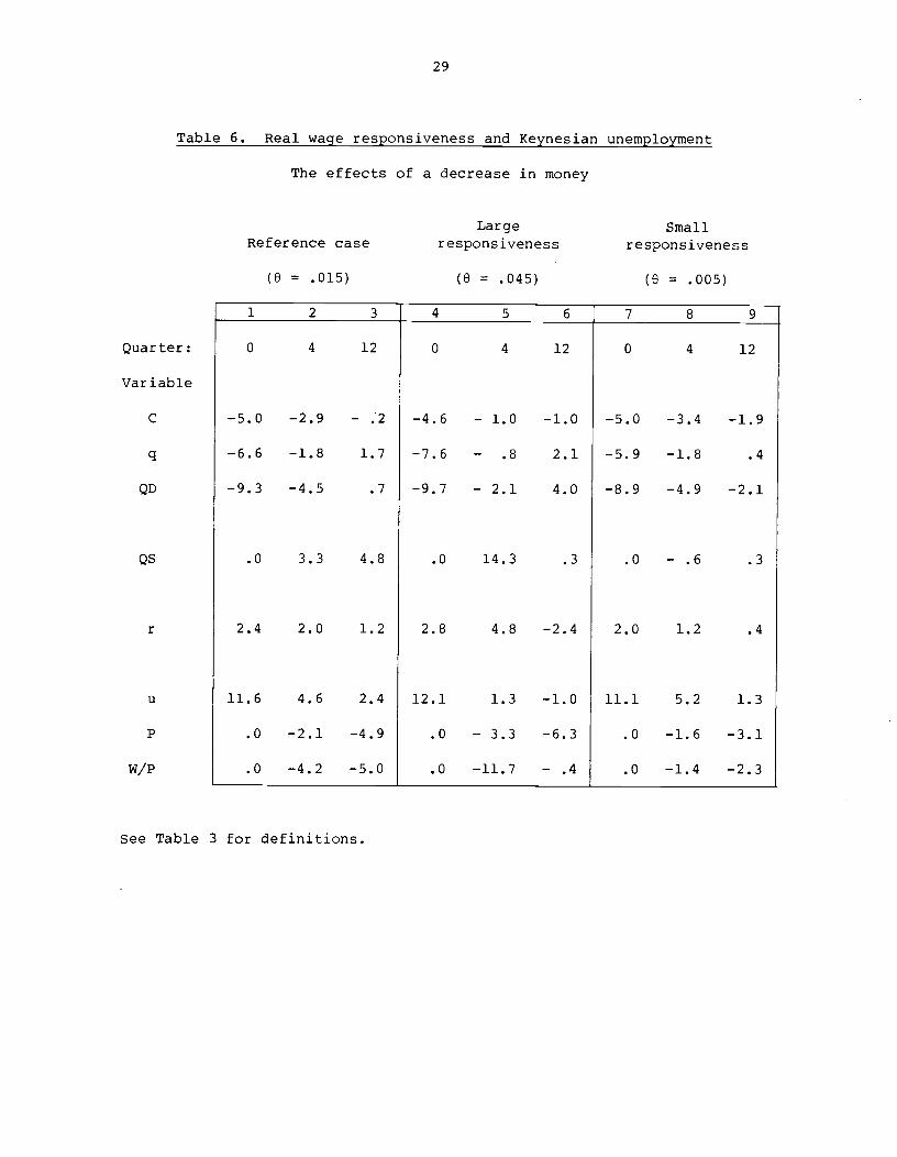
Simulation 4. Responsiveness of real wages and Keynesian unemployment

As emphasized by many authors, a decrease in the real wage is likely

to improve the economy in a classical regime but may well have perverse

effects in a Keynesian regime. We now consider the effects of real wage

responsiveness in such a case. Table 6 reports the effects of the decrease

in money, for three different values of 0, .005, .015 and .045.

Because of our formalization of consumers and our assumption of no

liquidity constraints, the distribution of output between profits and real

wages has no income distribution effect on consumption. Real wages however

have an effect on investment: For an output constrained firm, if real wages

are anticipated to be lower for a sufficiently long period of time, the firm

will aim at a lower capital/labor ratio and thus further decrease investment.

The result will therefore be a further decrease in aggregate demand.

This impact effect is there in Table 6. Large responsiveness of real

wages leads to a larger decrease in investment and aggregate demand; the

difference is however small across values of 0.

Of more interest is the process of adjustment which is not monotonic

but cyclical, due to the interaction of investment, output and real wages.

The initial period of recession and low investment is followed by a period

of expansion and higher investment. This is particularly clear when real

wages are very responsive. During this adjustment, aggregate demand is

sometimes larger than aggregate supply, as in column 6 and the economy

oscillates between Keynesian and classical regimes.

29

Table 6. Real wage responsiveness and Keynesian unemployment

Quarter:

Variable

C

q

QD

The effects of a decrease in money

See Table 3 for definitions.

Large SmallReference case responsiveness responsiveness

(8 = .015) (0 = .045) (0 = .005)

1 2 3 4 5 6 7 8 9

0 4 12 0 4 12 0 4 12

—5.0 —2.9 — .2 —4.6 — 1.0 —1.0 —5.0 —3.4 —1.9

—6.6 —1.8 1.7 —7.6 — .8 2.1 —5.9 —1.8 .4

—9.3 —4.5 .7 —9.7 — 2.1 4.0 —8.9 —4.9 —2.1

.0 3.3 4.8 .0 14.3 .3 .0 — .6 .3

2.4 2.0 1.2 2.8 4.8 —2.4 2.0 1.2 .4

11.6 4.6 2.4 12.1 1.3 —1.0 11.1 5.2 1.3

.0 —2.1 —4.9 .0 — 3.3 —6.3 .0 —1.6 —3.1

.0 —4.2 —5.0 .0 —11.7 — .4 .0 —1.4 —2.3

QS

r

U

P

w/P

30

We now turn to the effects of an anticipated profit tax.

Section III. Anticipations of a profit tax

The accession of a socialist government obviously creates large changes

in anticipations. Among those changes, two are likely to complicate the

task of economic policy initially. The first is the anticipation of large

budget deficits in the future, partially monetized and leading to higher

inflation. The second is the anticipation of lower profits by firms, either

because of higher real wages and compensation, or higher taxation of firms

(see Kolm [151). Although these anticipations may, in the case of France,

not be warranted, real and financial decisions based on them will affect

interest rates, the stock market, exchange rates as well as investment,

consumption and so on. An understanding of these anticipation effects is

important for the conduct of economic policy. In this section, we focus on

the effects of the anticipations of lower profits, summarizing the anticipa-

tions of various changes in the tax structure by an anticipation of a higher

tax rate on profits.

Taxes and the government budget constraint

For our purpose, we need to introduce only two taxes. The first is a

tax at rate T on profit 0 — (W/P)L. The second is a lump—sum tax or subsidy

on income. The government budget constraint is:

- T(Q — (W/P)L) + T = 0

An increase in T implies a corresponding decrease in T; thus a higher

profit tax does not, ceteris paribus, affect the income of consumers but

only its composition.

31

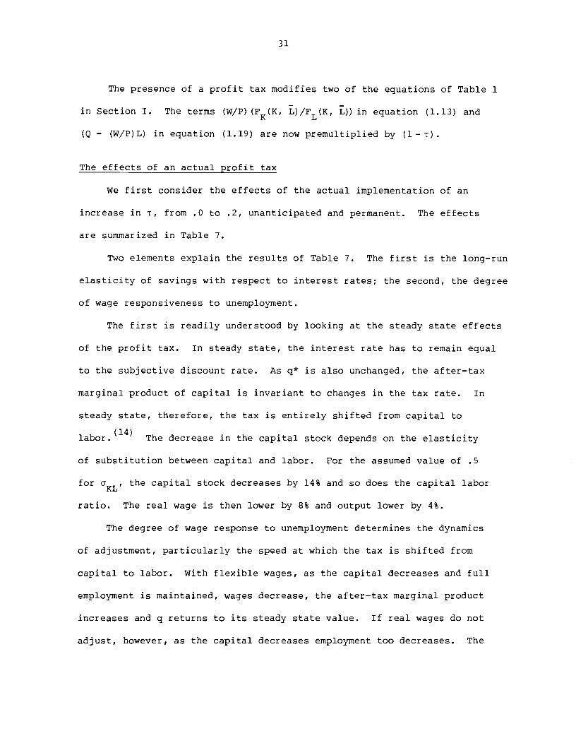
The presence of a profit tax modifies two of the equations of Table 1

in Section I. The terms (W/P) (FK(K, L)/FL(K, L)) in equation (1.13) and

(Q — (W/P)L) in equation (1.19) are now premultiplied by (l—T).

The effects of an actual profit tax

We first consider the effects of the actual implementation of an

increase in T, from .0 to .2, unanticipated and permanent. The effects

are summarized in Table 7.

Two elements explain the results of Table 7. The first is the long—run

elasticity of savings with respect to interest rates; the second, the degree

of wage responsiveness to unemployment.

The first is readily understood by looking at the steady state effects

of the profit tax. In steady state, the interest rate has to remain equal

to the subjective discount rate. As q* is also unchanged, the after—tax

marginal product of capital is invariant to changes in the tax rate. In

steady state, therefore, the tax is entirely shifted from capital to

labor. (14) The decrease in the capital stock depends on the elasticity

of substitution between capital and labor. For the assumed value of .5

for GKLI the capital stock decreases by 14% and so does the capital labor

ratio. The real wage is then lower by 8% and output lower by 4%.

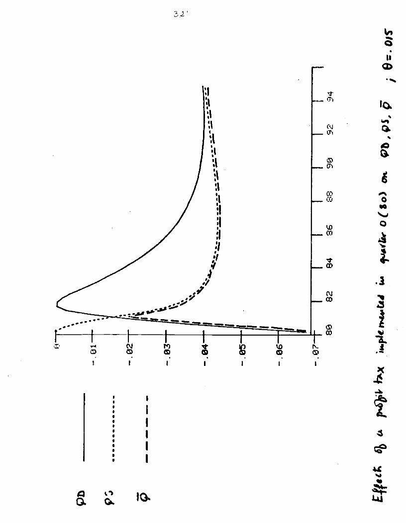
The degree of wage response to unemployment determines the dynamics

of adjustment, particularly the speed at which the tax is shifted from

capital to labor. With flexible wages, as the capital decreases and full

employment is maintained, wages decrease, the after—tax marginal product

increases and q returns to its steady state value. If real wages do not

adjust, however, as the capital decreases employment too decreases. The

32

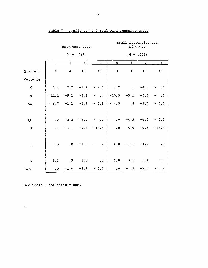
Table 7. Profit tax and real wage responsiveness

Small responsivenessReference case of wages

(0 = .015) (8 = .005)

1 2 3 4 5 6 7 8

Quarter: 0 4 12 40 0 4 12 40

Variable

C 1.4 2.2 —1.2 — 2.6 3.2 .1 —4.5 — 5.4

q —11.1 —5.1 —2.4 — .4 —10,9 —5.1 —2.8 — .8

QD — 6.7 —1.1 —1.3 — 3.8 — 4.9 .4 —3.7 — 7.0

QS .0 —2.3 —3.9 — 4.2 .0 —4.2 —6.7 — 7.2

K .0 —5.1 —9.1 —13.5 .0 —5.0 —9.5 —16.4

r 2.8 .8 —1.3 .2 4.0 —1.1 —1.4 .0

u 8.3 .9 1.6 .0 6.0 3.5 5.4 3.5

w/P .0 —2.0 —3.7 — 7.0 .0 — .5 —2.0 — 7.2

See Table 3 for definitions.

Pb

0050

0000

5 a

a —

a

— —

— —

— —

LV

80

£f!t;

6?,

4

$JI

spkn

444t

a4

p"'iO

(So)

at

9b,Q

S,

—.0

1

—.0

2

• a —

—

—

—

— C

—

—

—

.— —

82

84

86

88

90

92

94

I"

/

33

after—tax marginal product remains the same and g ernair below its steady

state value. In the extreme case of permanently fixc.d real .iages, this

conflict about income distribution leads to complete capital decumulation

over time, and zero employment. If El wages respond to unemployment, the

economy goes throg a protracted period of unemplornct arid capital

decumulation.

Table 7 shows that the adjustment takes the economy through two regimes.

The imposition of the tax leads to a decrease in investment demand and a

period of Keynesian unemployment (there are two conflicting effects on

consumption: the first is the anticipation of lower income, the second the

anticipation of constraints on future consumption spending. In the two cases

considered, the anticipatory buying effect dominates). As capital decumulates,

the economy enters a phase of classical unemployment (after 4 quarters in

the first case, 2 quarters in the second) , which lasts for more than 30

quarters in the first case, more than 50 in the second case. If the

responsiveness of real wages to unemployment is small, capital decumulates

below its new steady state level during the adjustment process.

The effects of an anticipated profit tax

Suppose now that the tax, instead of being currently implemented, is

anticipated for some time in the future. Table 8 reports the effects of

such anticipations. For both simulations, quarter 0 is the quarter in which

firms start anticipating the profit tax; this quarter may be the quarter of

the elections, or a prior quarter if the outcome of the elections was

anticipated. In the first simulation, the profit tax is anticipated for

8 quarters ahead and in the second simulation for 12 quarters ahead.5,16)

34

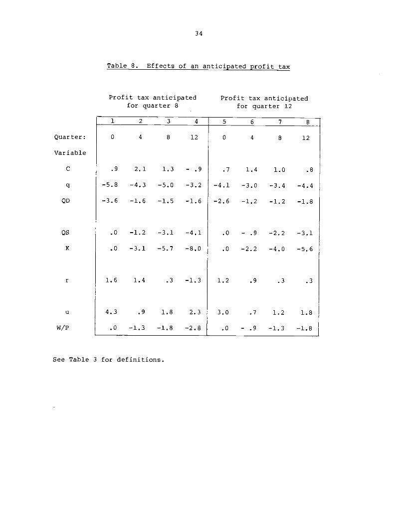
Table 8. Effects of an anticipated profit tax

See Table 3 for definitions.

Profit tax anticipatedfor quarter 8

Profit tax anticipatedfor quarter 12

0 4 8

1 2 3 4 5 6 7 8

0 4 8 12

.9

—5.8

—3.6

2.1

—4.3

—1.6

12

—.9

—3.2

—1.6

—4.1

—8.0

Quarter:

Variable

C

q

QD

QS

K

r

U

w/P

1.3

—5.0

—1.5

—3.1

—5.7

.0 —1.2

.0 —3.1

.7 1.4 1.0 .8

—4.1 —3.0 —3.4 —4.4

—2.6 —1.2 —1.2 —1.8

.0 — .9 —2.2 —3.1

.0 —2.2 —4.0 —5.6

.3 —1.31.6 1.4

4.3 .9 1.8 2.3

.0 —1.3 —1.8 —2.8

1.2

3.0

.9

.7

.3

1.2

.3

1.8

.0 — .9 —1.3 —1.8

PS

...

.....

.. —

. .

—

— —

— —

()

fec ' A

i (i'i

a) 0

.' 90

, Q

S,

I I $ I I $ S

—.0

1

—.0

2

—.0

4

80

84

86

90

92

94

35

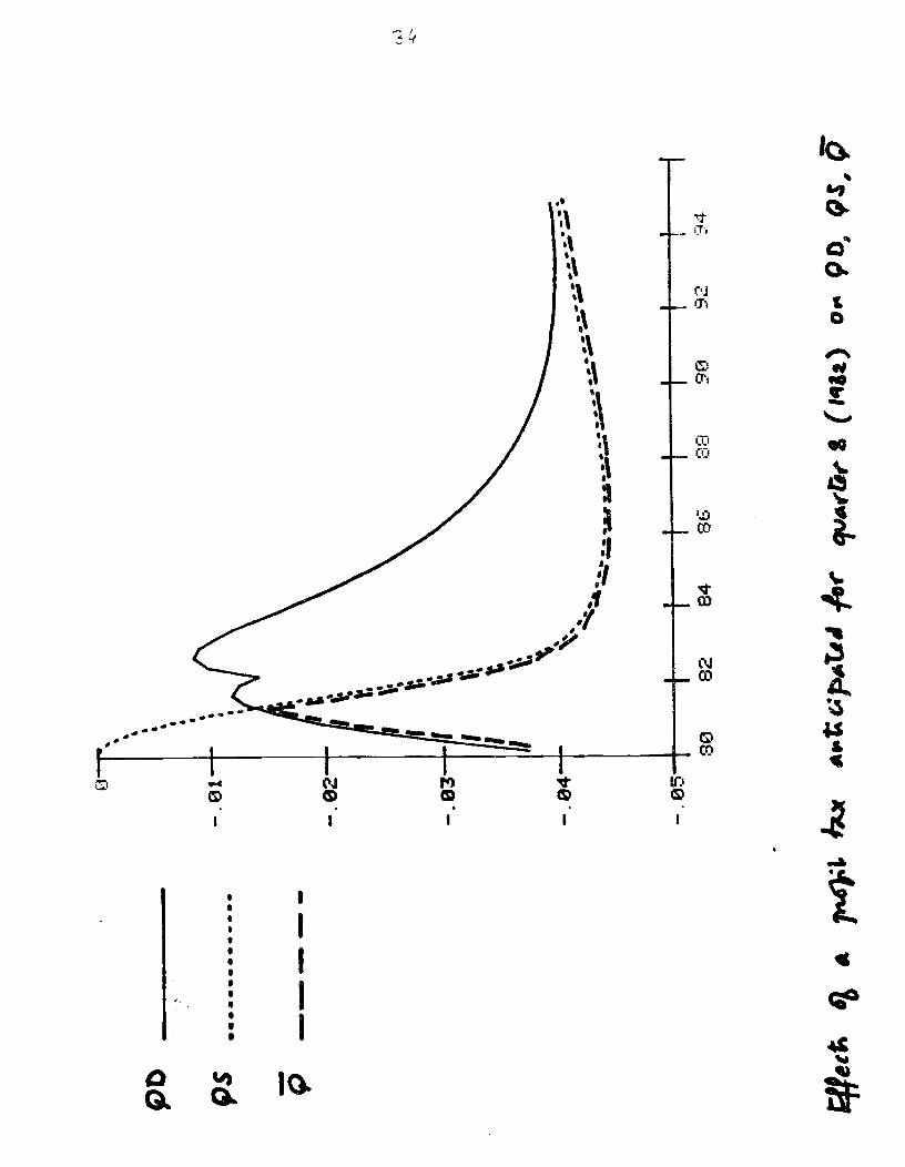
The effects are simple. The change in anticipation leads to a

substantial decline in investment (and a decrease in the stock market of

7% in the first case, 5% in the second). This decline in investment demand

leads to a Keynesian recession. As capacity decreases, the economy goes

into classical unemployment even before the profit tax is implemented. The

process of adjustment after the implementation is similar to the one

(17)described above.

Thus anticipations of a profit tax lead first to Keynesian unemployment,

then, later on, to classical unemployment. How can the government stabilize

employment, in the context of this model?

Most obviously, if the government does not plan an increase in profit

taxes, it may attempt to modify anticipations by the presentation of a

credible set of fiscal policies for the short and medium terms.

Second, the government may use a short—term expansionary policy to

avoid the initial recession, while anticipations of a profit tax disappear.

This may be done by measures to help either consumption or investment.

Helping consumption may not be successful if the economy is already close to

classical unemployment. Helping investment may increase both demand and

supply. Thus, the most successful policy may be, ironically, a temporary

reduction in the profit tax, which has effects both directly and as a signal

of the government's intentions,

36

Conclusion

The effect of a policy on the economy depends very much on whether it

has been anticipated or not, on how long it is expected to last and so on.

The model developed in this paper, which allows for rational firms and

households, as well as for imperfectly flexible prices, is well adapted to

characterize the effects of policy in such cases.

It is obviously too preliminary to be a reliable guide to policy: The

lack of foundations of price inertia, the infinite life assumption which

implies no income distribution effects, the closed economy assumption all

need to be relaxed. We believe however that, such as it is, it can shed

light on the effects of policy.

37

Footnotes

(1) We believe that models of price inertia will lead to price structures

in which relative prices, except for the real wage, are approximately

correct, but in which their average level, the price level, does not

adjust quickly. As this paper relies on price level and real wage

inertia only (and so implicitly assumes all other relative prices to

be flexible), we feel that results would not be drastically changed

by a more explicit derivation of price behavior.

(2) This strong assumption allows us to formalize agents and firms as

solving certainty problems. While convenient, and probably necessary

at this stage, it does not allow us to look at the effects of

uncertainty per se on behavior.

(3) Costs of adjustment are a simple way of deriving a well—behaved

flow investment demand. The specific functional form is a special

case of Lucas [17] which preserves CRTS of technology with respect to

K, L, I. This subsection builds heavily on Abel [1], Hayashi [131

and Blanchard [91.

(4) Considering the effects of a change in output only makes sense for an

output constrained firm. The "neoclassical" approach is slightly

confusing in this respect when it treats output as given, but maintains

the assumption that the wage equals the marginal product of labor.

(5) Around W/P = FL(KI L) and for L given by Q = F(K, L) the effect of a

change in output on marginal profit is given by:

((W/P) (FK(K, L)/FL(K, L))) = FK(K, L)/FL(K, L)aK

38

where cYKL is the elasticity of substitution between K and L. Thus,

the smaller GKL the larger the effects of a decrease in output on

marginal profit.

(6) An alternative formalization would be to solve for flexible prices

and wages and assume partial adjustment of actual prices and wages.

In the absence of more explicit assumptions about the source of price

and wage inertia, it is difficult to decide which formalization is

better.

(7) The time—separable utility function we use implies the same short— and

long—run elasticities of money demand with respect to both consumption

and interest rates.

(8) Actual estimates of this installation cost coefficient, b, derived from

regressions of investment on market value, are much higher. They are

however implausibly high and likely to be biased upwards (see {7]).

(9) Checking global stability before proceeding with simulations would be

desirable but is impossible. Checking local stability is feasible.

Stability conditions would combine the results of Blanchard and Kahn

[10] for linear systems with rational expectations and the results of

Ito [14] for systems with regimes and possibly discontinuous derivatives.

We have not checked them but have not encountered problems of convergence

in simulations.

(10) See footnote (5).

(11) There is inflation therefore only if there is excess demand for goods.

This assumption is acceptable only because we have assumed a zero rate

of growth of money. If this rate of growth were positive, the price

equations would have t be modited.

39

(12) The Mundell effect is currently felt in the U.S. where as the result of

lower money growth, high nominal rates and lower inflation have led to

short—term real rates around 8%.

(13) To reverse these results and obtain the Tobin result, the short—term

rate must have a strong impact on economic activity. This may be the

case if, for example, there are institutional restrictions in financial

markets, leading to rationing of specific sectors such as housing, when

short rates increase.

(14) The result that the interest rate remains unchanged and that the tax is

ultimately shifted to labor follows from the assumption that agents are——

or act as if they were——infinitely long lived. If agents have finite

horizons, the tax would only be partially shifted to labor. If, however,

the economy is small and open and there are no restrictions on capital

movements, the steady—state interest rate would again equal the foreign

interest rate and the tax would be fully shifted to labor.

(15) Firms are unlikely to have such precise anticipations. They are more

likely to think that the profit tax rate may be increased with some

probability which is an increasing function of time. We could formalize this

by considering the sequence of expected values of their subjective

distribution of tax rates. We could not however characterize the

effects of uncertainty per se on their behavior.

(16) If the government does not actually intend to increase the profit tax,

these simulations give only the anticipated future as of quarter 0.

If in quarter 8 in the first case (or 12 in the second) , there is no

increase in the profit tax and agents revise their anticipations, the

outcome in quarters 8 and followir; will be different from Table 8.

40

(17) In this case, excess shadow demand for goods is never very large and

thus there is no substantial inflation. It is however quite possible

to generate as a result of an adverse supply shock (profit tax,

increased price of some input or technological shock) , a period of

classical unemployment, a decrease in capital accumulation due to the

conflict in income distribution and substantial inflation as chronic

excess demand remains. Such an outcome may have some explanatory power

for what happened in the second half of the '70s.

41

References

[1] Abel, Andrew B. "Investment and the Value of Capital." Ph.D. thesis.Massachusetts Institute of Technology, 1978.

[21 __________ and Blanchard, Olivier J. "An Intertemporal Model of Savingand Investment." forthcoming Econometrica.

[3] Barro, Robert J. "Macroeconomic Analysis." mimeo 1981.

[4] __________ and Grossman, Herschel I. "Money, Employment andInflation." Cambridge: Cambridge University Press, 1976.

[5] Benassy, Jean Pierre "Neo—Keynesian Disequilibrium in a MonetaryEconomy." Rev. Econ. Studies 42 (1975): 503—523.

[6] Blanchard, Olivier J. "Output, the Stock Market and Interest Rates."A.E.R. 71 (March 1981) : 132—143.

[711 __________ "What is Left of the Multiplier—Accelerator?" A.E.R. 71(May 1981) : 150—155.

[8] __________ "Price Desynchronization and Price Level Inertia."R. Dornbusch and M. Simonsen (eds.). Indexation, Contractingand Debt in an Inflationary World. Cambridge: MIT Press,forthcoming.

[9] __________ "Dynamic Effects a Shift in Savings; the Role of Firms."forthcoming Econometrica.

[10] __________ and Kahn, Charles "The Solution to Linear DifferenceModels under Rational Expectations." Econometrica 48 (July 1980:1305—1313.

[11] Drèze, Jacques H. "Existence of an Exchange Equilibrium under PriceRigidities." Internat. Econ. Review 16 (June 1975): 301—320.

[12] Hall, Robert E. "The Macroeconomic Impact of Changes in Income Taxesin the Short and the Medium Runs." J.P.E. 86 (April 1978) S7l-85.

[13] Hayashi, Fumio "Tobin's Marginal q and Average q: A NeoclassicalInterpretation." Econometrica 50 (January 1982): 213—224.

[14] Ito, Takatoshi "Filippov Solutions of Systems of DifferentialEquations with Discontinuous Right Hand Sides." EconomicLetters 4—1979: 349—354.

[15] Kolm, Serge Christophe "La Transition Socialiste." Paris: CERF,1977.

42

[161 Lipton, David, Poterba, James, Sachs, Jeffrey and Summers, Lawrence"Multiple Shooting in Rational Expectations Models." forthcomingEconometr ica.

[17] Lucas, Robert E. "Adjustment Costs and the Theory of Supply." J.P.E.75 (August 1967): 321—334.

[18] __________ "Studies in Business Cycle Theory." Cambridge: MIT Press,1981.

[19] Malinvaud, Edmond "The Theory of Unemployment Reconsidered." Oxford:Basil Blackwell, 1977.

[20] _________ "Profitability and Unemployment." Cambridge: CambridgeUniversity Press, 1980.

[211 Neary, Peter J. and Stiglitz, Joseph E. "Expectations and ConstrainedEquilibria." forthcoming Q.J.E.

[22] Sachs, Jeffrey "Energy and Growth under Flexible Exchange Rates."J. Bhandari and B. Putnam (eds.). The International Transmissionof Economic Disturbances. Cambridge: MIT Press, forthcoming.

[23] __________ "Wages, Profits and Macroeconomic Adjustment: A ComparativeStudy." Brookings Papers on Econ. Activity 2 (1979): 269—319.

[241 Sargent, Thomas J. "Macroeconomic Theory." New York: Academic Press,1979.

[25] Taylor, John "Staggered Wage Setting in a Macro—Model." A.E.R. 69(May 1979) : 108—113.

[26] Tobin, James "Keynesian Models of Recession and Depression." A.E.R.65 (May 1975) : 195—202.