Natural Rate of Interest in Japan –– Measuring its size and identifying drivers based on a DSGE model –– Yosuke Okazaki* yousuke.okazaki@boj.or.jp Nao Sudo** nao.sudou@boj.or.jp

No.18-E-6 March 2018

Bank of Japan 2-1-1 Nihonbashi-Hongokucho, Chuo-ku, Tokyo 103-0021, Japan

**Monetary Affairs Department **Monetary Affairs Department

Papers in the Bank of Japan Working Paper Series are circulated in order to stimulate discussion and comments. Views expressed are those of authors and do not necessarily reflect those of the Bank. If you have any comment or question on the working paper series, please contact each author.

When making a copy or reproduction of the content for commercial purposes, please contact the Public Relations Department (post.prd8@boj.or.jp) at the Bank in advance to request permission. When making a copy or reproduction, the source, Bank of Japan Working Paper Series, should explicitly be credited.

Bank of Japan Working Paper Series

Natural Rate of Interest in Japan

-- Measuring its size and identifying drivers based on a DSGE model --

Yosuke Okazaki† and Nao Sudo‡

March 2018

Abstract

In this paper, we explore the level and determinants of the natural rate of interest in Japan. To

this end, we construct a DSGE model that is specifically designed to address potential drivers

of the natural rate that are considered important in previous studies, and estimate the model

using Japan's data from 1980 to 2017. Our findings are summarized in the following three

points. First, the natural rate has shown a secular decline over time, from 400 basis points in

the 1980s, to 30 basis points in the last five years. The decline has been mostly attributed to

changes in neutral technology. Changes in investment-specific technology, working-age

population, and demand factors have also contributed to the decline, but the quantitative

impacts have been small. Second, a secular decline and the quantitative importance of neutral

technology are also seen when considering the expected future natural rates over a long

horizon, indicating that changes in the natural rate have been perceived as persistent rather

than temporal changes over the course of history. Third, in the banking crisis starting in the

1990s, financial factors stood out as an important driver that depressed the natural rate. Their

contribution holds second place, after changes in neutral technology, when comparing

potential drivers by the size of their contribution to variations in the natural rate. Our results

suggest the need to monitor the financial intermediation function, as well as the path of

neutral technology when analyzing developments in the natural rate.

JEL classification: E32; E43; E44; E52

Keywords: Natural Rate of Interest; Monetary Policy Implementation; DSGE Model

The authors would like to thank Kosuke Aoki, Hibiki Ichiue, Takushi Kurozumi, Teppei Nagano, Jouchi Nakajima, Kenji Nishizaki, Masashi Saito, Toshiaki Watanabe, Toshinao Yoshiba, and seminar participants at the Bank of Japan, for their useful comments. The views expressed in this paper are those of the authors and do not necessarily reflect the official views of the Bank of Japan. † Monetary Affairs Department, Bank of Japan (E-mail: yousuke.okazaki@boj.or.jp) ‡ Monetary Affairs Department, Bank of Japan (E-mail: nao.sudou@boj.or.jp)

1 Introduction

The natural rate of interest (hereafter the natural rate) is the real interest rate at which

economic activity and prices neither accelerate nor decelerate. Close monitoring of devel-

opments in the natural rate is essential for monetary policy implementation, since, with

almost no exceptions, monetary easing is attained by driving the real interest rate below

the natural rate. There are, however, some di¢ culties associated with monitoring the nat-

ural rate in practice. The natural rate is not observable and needs to be estimated, while

the rate is considered to vary over time, re�ecting changes in the economic environment

that a¤ect the savings and investment decisions of �rms and households.

Broadly speaking, there are two approaches to estimating the natural rate. In the �rst

approach, the natural rate is distilled as the trend component of the actual real interest rate,

using the Hodrick-Prescott �lter, a band-pass �lter, or other more sophisticated time series

methodologies. The estimation process often exploits the time series of the real interest rate

alone, and the theoretical relationship with other variables, such as prices and the output

gap, is not taken into account. In the second approach, the natural rate is estimated as the

hypothetical real interest rate that is consistent with a theoretical requirement such as that

stipulated above, using a structural economic model that exploits the data of variables other

than interest rates. One widely used framework in this category is the approach developed

by Laubach and Williams (2003, hereafter LW).1 Another extensively used framework in

this approach is a dynamic stochastic general equilibrium (hereafter DSGE) model.2 One

advantage of using DSGE models is that, along with the theoretical consistency of the

models, it uncovers the nature of the underlying drivers of the natural rate and helps form

clear structural interpretations of their dynamics.3

In this paper, we estimate the time path and drivers of the natural rate in Japan from

1980 to 2017, using a New Keynesian DSGE model. Following convention, we de�ne the

1See Fries et al. (2016), Pescatori and Turunen (2016), Lewis and Vazquez-Grande (2017), and Hakkioand Smith (2017) for estimates based on the approach of LW (2003). See also Holston et al. (2017), whoapply the LW methodology to the U.S., Canada, the euro area, and the U.K.

2Work based on DSGE models includes, for example, Edge et al. (2008), Justiniano and Primiceri(2010), Barsky et al. (2014), Curdia et al. (2015), Del Negro et al. (2015, 2017), Hristov (2016), and Geraliand Neri (2017).

3 In addition to the two approaches listed here, some studies, such as Ikeda and Saito (2014), and Sudoand Takizuka (2018), use a calibrated general equilibrium model and compute the real interest rate byfeeding into the model the time path of key exogenous variables such as demographic factors and TFP. Seealso Carvalho et al. (2016) and Gagnon et al. (2016) for related analyses.

1

natural rate as the ex-ante real short-term interest rate that would prevail if all prices and

wages are �exible. Most studies on the natural rate in developed countries agree that the

rate has fallen over the years, particularly in the wake of the recent global �nancial crisis.

By contrast, there is less agreement as to what has been the dominant driver of the natural

rate over the course of history. We have therefore been careful in our choice of analytical

framework so that our analysis not only pins down the level of the natural rate but also

serves as a horse racing of potential drivers. That is to say, we focus on selected drivers

that have already been proposed and have so far attracted considerable attention in the

literature. They are neutral technology, investment-speci�c technology, �nancial factors,

demographic factors, and demand factors. We design the settings of our DSGE model

and our estimation strategy so that the quantitative impacts of these drivers are explicitly

addressed in the model and the relevant information on these drivers is appropriately used

in the estimation.4

In addition to the natural rate, similar to Justiniano and Primiceri (2010), we compute

the sequence of expected future natural rates over a long horizon, which we refer to as the

expected natural rates, and study how they respond to changes in each driver and how

they have evolved over time. This is because this measure summarizes how long a change

in the natural rate taking place in the current period will last and serves as a metric for

comparing the relative importance of drivers.5

We �nd that the natural rate in Japan shows a decline from about 400 basis points

in the 1980s, to 30 basis points in the last �ve years. The decline was most pronounced

in the �rst half of the 1990s and became moderate in subsequent years. As of 2017, the

estimated level of the rate is about 100 basis points. The estimated declining rate accords

well with the estimate of the natural rate in Japan based on alternative methodologies

such as that of LW (2003) and Imakubo et al. (2015), or estimates based on other DSGE

models (Iiboshi et al. [2017]). In our estimate, more than half of the decline is attributed to

4Model selection is essential when estimating the level and determinants of the natural rate. Hristov(2016) estimates the natural rate in the euro area using two di¤erent DSGE models, a variant of Smets andWouters (2007), and the same model but equipped with �nancial frictions. He documents that the size ofthe estimated decline in the natural rate during the global �nancial crisis was about 400 basis points in theformer, and about 200 basis points in the latter; while the dominant driver of the natural rate was shocksto the discount factor in the former, and shocks to the rate of return on capital in the latter.

5As examined in Justiniano and Primiceri (2010), it also serves to gauge the degree of monetary policyimplementation. The importance of looking at the expected natural rates over a long horizon is warrantedin particular when the prevailing nominal short-term interest rate is �oored and alternative policy measurestargeting expectations, such as forward guidance, are adopted in monetary policy implementation.

2

changes in neutral technology. Changes in the working-age population, investment-speci�c

technology, and demand factors have also contributed to the decline, but their quantitative

impacts have been limited. Financial factors have driven the natural rate cyclically over

the sample period. They dampened the natural rate about 100 basis points during the

banking crisis, and enhanced the rate in the years after 2000. When compared by size of

contribution to variations in the natural rate, shocks to �nancial factors hold second place

among the �ve drivers, after the contribution of shocks to neutral technology.

Similar to the natural rate, the expected natural rate also exhibits a decline over the

sample period, suggesting that the natural rate decline over time has been perceived as

persistent rather than as temporal changes by agents in the economy. This in part re�ects

the fact that the bulk of variations in the natural rate have been driven by changes in neutral

technology whose e¤ects on the natural rate are long-lived. The decline has taken place

more gradually, closely tracking the time path of the potential growth rate, particularly in

recent years.

Our study is related to studies that estimate the natural rate in various economies, in

particular those that use DSGE frameworks. These analyses include Barsky et al. (2014)

and Del Negro et al. (2015, 2017) for the U.S., Hristov (2016) for the euro area, Goldby et

al. (2015) for the U.K., and Iiboshi et al. (2017) for Japan. Our paper is also related to

works on the secular stagnation hypothesis, including Eggertsson et al. (2017), Rachel and

Smith (2015), Sajedi and Thwaites (2016), and Summers (2014). Since the remark made

by Summers (2013), growing attention has been paid to the question whether the natural

rate has merely been declining thus far, or will continue to decline, and if so, why. The �ve

drivers focused on in this paper are all included in the lists in existing studies of potential

causes of the decline. Lastly, the current paper is related to studies that estimate a DSGE

model using Japan�s data, including Sugo and Ueda (2008), Kaihatsu and Kurozumi (2014),

Hirakata et al. (2016), and Muto, Sudo, and Yoneyama (2016, hereafter MSY). Our study

is close to Hirakata et al. (2016) and MSY (2016) in terms of model settings, in particular

those associated with �nancial frictions.

The contribution of our paper is as follows. First, it provides the time path and drivers

of the natural rate over the years in Japan, using a New Keynesian model. To the best

of our knowledge, this paper is currently the only paper that estimates the natural rate in

3

Japan using a medium-scale DSGE model with a �nancial friction.6 Second, it focuses on a

broad set of drivers considered essential in previous studies, and assesses their quantitative

implications for the current natural rate and future expected natural rates, using a model

speci�cally designed for this purpose. We give a chance not only to temporary shocks such

as demand shocks but also to long-lived shocks such as growth rate shocks to technology to

account for both current and future natural rates, and compare their roles. In particular,

our paper di¤ers from existing studies in quantifying the impact of key drivers on expected

future natural rates over a long horizon.

The remainder of this paper is organized as follows. Section 2 summarizes the potential

drivers of the natural rate discussed in existing studies. Section 3 provides an overview of

our model and the estimation strategy. Section 4 reports the estimation results. Section 5

is devoted to the validation check and sensitivity analysis. Section 6 concludes.

2 Potential Drivers of the Natural Rate

In this section, we describe the potential drivers of the natural rate. There are already a

number of studies on this topic, in particular in relation to the secular stagnation hypothesis

advocated recently by Summers (2013). Here, for the convenience of the analysis below,

we classify the drivers into �ve categories and describe how each driver a¤ects the natural

rate. We also brie�y discuss the implications for Japan�s economy and how we design our

model and estimation settings so as to address and quantify these drivers.

Neutral technology

According to the text book growth model, changes in neutral technology are the key

source of macroeconomic �uctuations, including those of real interest rates. While neutral

technology itself is not directly observable, in developed countries, there is evidence that

neutral technology has recently grown at a slower pace than before, as documented for

example in Cette et al. (2016) and Eichengreen et al. (2017). Theoretically, stagnation

in neutral technology reduces the return on capital, making investment less pro�table.

6The di¤erence between the estimates by Iiboshi et al. (2017) and our estimates is that, while bothare based on a DSGE model, they keep their model framework simple and estimate the model explicitlyaddressing the non-linearity associated with a zero lower bound of the policy rate. By contrast, while ourpaper incorporates fairly rich ingredients into the model, such as �nancial frictions and endogenous changesin the measured TFP, it disregards the non-linearity addressed in their paper.

4

Consequently, to the extent that a lower return on capital discourages investment, real

interest rates should fall. Somewhat surprisingly, however, in most existing estimates

based on a DSGE model, a change in neutral technology does not manifest itself as the

key driver of the natural rate.7

In Japan, as documented in a pioneering paper by Hayashi and Prescott (2002), there

was a kink around the early 1990s in the growth rate of measured TFP, the widely agreed

proxy of neutral technology in the literature. The growth rate of the measured TFP was

on average 1.84% in the 1980s, dropping to 0.49% in the 1990s and 0.46% in the 2000s and

beyond, suggesting that changes in neutral technology growth rates may have contributed

negatively to developments in the natural rate over the last forty years.

To see if this interpretation holds true, we employ three ingredients in our analysis:

First, we incorporate a stochastic trend to neutral technology, similar to previous studies,

including Gerali and Neri (2017). Second, we use the time series of measured TFP, the

Solow residual, in estimating our model. As discussed in Basu et al. (2006), however,

the measured TFP can be driven not only by changes in neutral technology but also by

non-technological factors, such as demand shocks, if the actual production process involves

the use of intermediate inputs or endogenous changes in capacity utilization of production

inputs. As the third element, therefore, we explicitly incorporate these elements when

modeling production function of goods producers.

Financial factors

Existing estimates mostly agree that the natural rate in developed countries discon-

tinuously plummeted at the outset of the global �nancial crisis in 2007.8 It is therefore

natural to see �nancial factors as an important potential driver of the natural rate. When

�nancial intermediation malfunctions, the amount of borrowing by �rms and households

should fall, and (risk-adjusted) real interest rates may fall, too. For example, according

to an estimate by Goldby et al. (2015), about 400 basis points decline in the natural rate

in the U.K. during the period of the global �nancial crisis was attributed to risk premium

shock, which in their interpretation represents credit supply shocks.

7One possible reason is because some studies assume that the trend component of neutral technologyevolves deterministically and focus only on the e¤ects of changes in the stationary component of neutraltechnology.

8See, for example, Holston et al. (2017) for estimates based on the methodology of LW (2003), andBarsky et al. (2014) and Del Negro et al. (2015) for estimates based on a DSGE model.

5

In Japan, there have been two crises in the last forty years; the banking crisis that

started with an asset price collapse in the early 1990s, and the global �nancial crisis.

The �rst crisis damaged the balance sheets of �nancial intermediaries (hereafter FIs) and

goods producers, and banks�credit cost rate climbed up to 3.7% at its peak, leading to

disruptions to �nancial intermediation and the collapse of large �nancial institutions in

1997 and beyond.9 According to the dating by Reinhart and Rogo¤ (2011), this banking

crisis persisted from 1992 to 2001. The latter crisis was not accompanied by a �nancial

turmoil in Japan. It did, however, trigger a slump in the economy. GDP fell by 8.29%

from the peak of the business cycle in 2008:1Q, to the trough in 2009:1Q.10

In order to address �nancial factors, we follow Hirakata, Sudo, and Ueda (2011, 2017,

hereafter HSU) and incorporate what they call a chained credit contract into the model.

In this framework, both non-�nancial �rms and FIs are credit constrained, raising external

funds through credit contracts similar to those adopted in Bernanke, Gertler, and Gilchrist

(1999, hereafter BGG).11 FIs lend to non-�nancial �rms what they borrow from households

and their own net worth, and the non-�nancial �rms invest in capital goods, using what

they borrow from FIs and their own net worth. Following HSU (2011, 2017), we incorporate

shocks to the balance sheets of the two sectors, and these are referred to as �nancial shocks

in the paper. They are shocks to the net worth accumulation of these sectors, and a¤ect

macroeconomic variables primarily by changing the terms of the credit contracts. With

these shocks, we intend to capture changes in �nancial intermediation that arise not from

macroeconomic conditions, but from �nancial factors.12 In addition, when estimating the

model, we employ the net worth series for FIs and non-�nancial �rms using the Flow of

Funds data, so as to accurately estimate the time path of shocks to the net worth over

9See Hoshi and Kashyap (2010) for the sequence of events during this crisis period. See also Bayoumi(2001), for example, for the quantitative impact on economic activity of disruption to �nancial intermedi-ation during this period.10Here, we follow the dating of Japanese business cycle released by the Cabinet O¢ ce. The recession that

has coincided with the global �nancial crisis corresponds to the 14th business cycle based on the dating.11The �nancial accelerator framework of BGG (1999) is commonly used in existing studies that estimate

the natural rate with a DSGE model with a �nancial friction. See, for example, Del Negro et al. (2017)and Hristov (2016). Another type of �nancial friction used in the literature is the one used in Eggertssonet al. (2017). In their model, households are subject to borrowing constraint, and an exogenous change inthe degree of the constraint reduces the natural rate even to a level below zero.12Existing studies, such as Gilchrist and Leahy (2002) and Nolan and Thoenissen (2009), also consider

shocks that are similar in nature to our net worth shocks. Their interpretations of these shocks include�asset bubble and burst of asset bubble,��irrational exuberance,�or �innovation in the e¢ ciency of creditcontracts.�

6

time.

Demographic landscapes

Population aging and real interest rate declines have gone hand-in-hand over the last

few decades in developed countries. Based on this observation, there are a growing number

of studies that explore the relationship between real interest rates and demographic factors

using a calibrated life-cycle model. These include Carvalho et al. (2016), Gagnon et al.

(2016), and Sudo and Takizuka (2018). These studies commonly show that population

aging, arising from a declining fertility rate, increasing longevity, or both, depresses real

interest rates, since a lower fertility rate is translated into lower labor inputs, and increased

longevity increases the amount of capital inputs by giving households added incentive to

save.

As documented in Sudo and Takizuka (2018), among the G7 countries, population aging

is most pronounced in Japan. In their estimate, from 1980 to 2017, the growth rate of the

working-age population has declined by 1.86%, from 0.84% to -1.03%, and life-expectancy

has risen by 7.2 years, from 77.2 to 84.4 years in Japan; whereas in the U.S., for example,

the corresponding numbers are 1.27% and 3.7 years.

Existing estimates using a DSGE model do not address demographic factors, in part

because these factors are considered as primarily a¤ecting the low-frequency components of

macroeconomic variables, and in part because some demographic changes are predictable.

In the analysis below, we incorporate one element of demographic factors into the model,

following Burriel et al. (2010), and study its e¤ect on the natural rate. Namely, we

assume that the working-age population evolves stochastically by incorporating shocks to

the growth rate of the working-age population, allowing macroeconomic variables, including

the natural rate, to react to these shocks. In estimating the model, we use the actual

working-age population growth rates to extract the demographic shocks.

Investment-speci�c technology

Since the pioneering work by Greenwood, Hercowitz and Krusell (1997) document-

ing the evidence of advances in investment-speci�c technology over the years in the U.S.,

investment-speci�c technology has been considered an important driving force of macro-

7

economic variables.13 An improved investment-speci�c technology makes the price of in-

vestment goods cheaper. On the one hand, this implies that a smaller amount of �nal

goods is needed to make the same size of investment, which in turn depresses real interest

rates. On the other hand, if the technological improvement induces a larger investment,

it should rather boost real interest rates. Whether the former e¤ect dominates the lat-

ter depends on whether capital and labor inputs are complements or substitutes in goods

production. Sajedi and Thwaites (2016) show, using an overlapping generations (hereafter

OG) model where the two production inputs are complementary, that improvements in

investment-speci�c technology reduce the relative price of capital goods, and depress real

interest rates.

Changes in investment-speci�c technology are often measured through changes in the

relative price of investment goods. In Japan, based on the investment de�ator divided by

the GDP de�ator, the relative price grew at an average rate of -0.64% from the 1980s to

2017. The growth rate was -1.18% on average during the two decades ending in 2000, and

was 0.20% in the rest of the sample period, suggesting that investment-speci�c technology

advanced markedly in the 1980s and 1990s, and slowed down in the subsequent years. We

explicitly incorporate into the model investment-speci�c technology that grows stochasti-

cally, following the speci�cation of Fisher (2006), so that changes in the technology a¤ect

macroeconomic variables, including the natural rate, and use the time series of the relative

price of investment goods as an observable when estimating the model. Following conven-

tion, however, we maintain the assumption that the price elasticity of capital and labor

inputs is unity in the model.

Demand factors

Changes in household demand, in particular shocks to discount factor, have been consid-

ered important drivers of the natural rate. While there is no agreement as to why demand

structure changes shape, some existing studies point out that a compositional change in

households with di¤erent characteristics, in terms of age or wealth, may alter the demand

structure of the household sector as a whole. Demand factors are regarded as the key

driver of natural rates in some studies. For example, Iiboshi et al. (2017) document that

13See, for example, the early work by Fisher (2006) that evaluates the importance of investment-speci�ctechnology shocks using a growth model.

8

the bulk of variations in the natural rate from the 1980s to the present in Japan have been

brought about by changes in discount factor. To address demand factors, we incorporate

two types of demand shocks: shocks to discount factor and to external demand. Because

these demand shocks themselves are not observable, we do not employ speci�c variables

for extracting demand shocks in our estimation procedure.

3 Model Description and Estimation Procedure

3.1 Model Overview

Most of the settings in our model are borrowed from existing studies including HSU (2011)

and MSY (2016). In this section, we therefore provide a model overview together with

the selected key elements of the model, including how the working-age population changes

and a¤ects households�decisions, how monetary policy is implemented, the nature of fun-

damental shocks, and the de�nition of the natural rate in the model. We describe the

full model structure in Appendix A. See also Figure 1, where the outline of the model is

graphically depicted.

Compared to the standard New Keynesian model, such as that in Smets and Wouters

(2007), our model includes the following additional elements.

1. Stochastic trends in neutral technology and investment-speci�c technology.

2. Stochastic trends in the working-age population, following Burriel et al. (2010).

3. Credit contracts between households and FIs, following HSU (2011) and MSY (2016).

4. Credit contracts between FIs and entrepreneurs, or equivalently non-�nancial �rms,

following HSU (2011) and MSY (2016).

5. Intermediate inputs and endogenous capacity utilization of capital stock, following

Basu (1995) and MSY (2016).

6. Anticipated shocks to short-term nominal interest rates in the future, following Laseen

and Svensson (2011) and Del Negro et al. (2017).

The �rst to �fth elements are incorporated so as to correctly address the potential

impacts of the �ve drivers of the natural rate. The last element typically serves to separately

9

quantify the impact of forward guidance in existing studies. As discussed in Section 5,

however, this speci�cation is also intended to serve in accurately estimating the natural

rate in this paper.

3.1.1 Changes in Working-age Population

In our model, there is a continuum of households, and each household is composed of

Ht identical workers. Each household decides how much each worker works, consumes,

and saves so as to maximize the sum of the expected life-time utility of each household

member. While existing studies based on a New Keynesian DSGE model often assume that

the number of workers Ht grows in a deterministically manner or is unchanged over time,

some portion of changes in its growth rate in a period t are in fact unpredictable in a period

t� 1 in the actual economy. We therefore assume, following Burriel et al. (2010), that the

working-age population grows stochastically, subject to the law of motion described below:

lnHt = lnHt�1 + �H;t;

where �H;t is a shock to the growth rate of workers.

Upon the arrival of a shock to the working-age population growth rate, each household

changes its decisions about hours worked, consumption, and saving, which in turn a¤ects

allocations and prices including the natural rate. For example, denoting the aggregate

labor input, hours worked by each worker at a household h by Lt and lt (h) ; other things

being equal, a positive shock to the growth rate mechanically increases the size of the

aggregate labor inputs, since the following equality holds.

Lt = Ht � lt (h) :

If the usages of the other production inputs are unchanged, this change makes capital

inputs relatively scarce, boosting the real interest rates in the economy.

It is notable that this setting implicitly assumes that the entire change in working-age

population growth is unknown. We choose this setting because how expectation about

future working-age population growth is formed in practice is not obvious. Our strategy

is therefore to give the largest chance to shocks to the working-age population growth

to explain the natural rate by simply assuming there is no anticipated component in the

10

growth rate. In later section, we relax this assumption and study how the results are

altered when di¤erent speci�cations about the growth rates are assumed.

3.1.2 Monetary Policy

Monetary policy implementation in our model is standard, except that it includes antici-

pated nominal interest rate shocks. As studied in Laseen and Svensson (2011), these shocks

can work in a manner di¤erent from unanticipated shocks. We incorporate them because

our sample period covers a period when short-term nominal interest rates were around

zero, and forward guidance was used as part of monetary policy implementation.

The central bank adjusts the policy rate according to the following Taylor rule with

a time-varying target rate of in�ation and the exogenous component of the policy rule as

described below:

Rn;t = R�n;t�1

�R��

��t��t

�'��1��exp (�t) ; (1)

where

�t = �Rn;t + "Rn;1;t�1 + "Rn;2;t�2 + :::+ "Rn;S ;t�S : (2)

Here, Rn;t is the nominal interest rate, �t is the in�ation, � 2 (0; 1) is the interest rate

smoothing parameter of the monetary policy rule, '� > 1 is the policy weight attached to

the in�ation rate, R�is the steady state natural rate, � is the steady state in�ation rate,

and ��t is the target rate of in�ation that varies according to the following equation;

ln ��t = (1� ��) ln �� + �� ln ��t�1 + ��;t:

Here, �� 2 (0; 1) is the autoregressive coe¢ cient and ��;t is a shock to the target rate of

in�ation. Note that �t is a shock to the monetary policy rule, and is decomposed into the

unanticipated component and anticipated component. The unanticipated component �Rn;t

is an i.i.d. shock, and anticipated policy shocks "Rn;s;t�s; s = 1; 2; :::; S are known to agents

at period t� s in advance, but each of the shocks materializes in the policy rule with a lag

of s quarters.

11

3.1.3 Fundamental Shocks

The model consists of fourteen fundamental shocks and S number of anticipated monetary

policy shocks. For our purposes, they are categorized into the following six groups.

1. Shocks to neutral technology: these are shocks that directly a¤ect the neutral produc-

tion technology of the gross output Yg;t, and there are both long-lived and short-lived

shocks, denoted as �Za;t and �Aa;t; respectively.

2. Shocks to investment-speci�c technology: these are shocks that a¤ect capital goods

production technology exclusively. Similar to neutral technology shocks, there are

both long-lived and short-lived shocks, denoted as �Zd;t and �Ad;t; respectively.

3. Shocks to the net worth of FIs and entrepreneurs: these are shocks that a¤ect the

accumulation of retained earnings and therefore net worth in the two sectors NF;t

and NE;t. Positive net worth shocks enhance the balance sheet conditions of these

sectors, and negative shocks work in the opposite direction. These shocks are denoted

as �NF ;t and �NE ;t; respectively.

4. Shocks to the working-age population growth rate: these are shocks that change the

working-age population growth rate. Because they a¤ect the growth rate, their im-

pact on the level of the working-age population lasts permanently. They are denoted

as �H;t:

5. Shocks to demand factors: these are shocks to discount factor and shocks to external

demand, denoted as �d;t and �G;t; respectively.

6. Other shocks: these are shocks that are not categorized above, including shocks to the

investment adjustment cost ZI;t; the price markup �PY ;t; the wage markup �W;t; the

target rate of in�ation ��t; and both unanticipated and anticipated monetary policy

shocks �Rn;t and "Rn;s;t�s; s = 1; 2; :::; S:

3.1.4 De�nition of the Natural Rate

The natural rate

We de�ne the natural rate R�t as the ex-ante real short-term interest rate that would

prevail in a counterfactual economy, which we call the �exible-price economy. The �exible-

price economy is exactly the same as the actual economy described in Appendix A, except

12

that both wages Wt and prices Pt are perfectly �exible and there are no markup shocks.14

In other words, in this �exible-price economy, the parameters associated with adjusting

nominal prices are zero, �w = �p = 0 and markup shocks are zero �W;t = �PY ;t = 0 for all

t. In what follows, we denote as X�t the �exible-price economy counterpart of a variable

Xt in the actual economy.

As already discussed in existing studies, such as Justiniano and Primiceri (2010) and

Barsky et al. (2014), the di¤erence between the prevailing ex-ante real interest rate Rt

and the natural rate R�t can be used as a metric when measuring the degree of monetary

easing. Denoting the deviation of a variable Xt (or X�t ) from the steady state by ~Xt (or

~X�t ), the Euler equation of the households in our model can be arranged to the following

expression.15

~ct � ~c�t = �1Xs=0

Et�~Rt+s � ~R�t+s

�: (3)

Here Et is the expectation operator. Note that the gap between the actual economy and

that in the �exible-price economy is closed when the sum of the sequence of the expected

real interest rate ~Rt+s from the current period to the in�nite future coincides with that of

the natural rate ~R�t+s over the same period.16

The natural rate at the steady state

The natural rate varies in response to various shocks listed above other than monetary

policy shocks and markup shocks. At the steady state, however, the natural rate is deter-

mined by the households�discount factor �; and the growth rates of neutral technology and

investment-speci�c technology. Denoting the value of a variable Xt at the non-stochastic

steady state as Xss, from the Euler equation, we have:

Rss = R�ss =1

�g

1(1� )(�+�E+�F )Za;ss

g(1����E��F )�+�E+�F

Zd;ss=1

�� ; (4)

14Similar to the settings in Barsky et al. (2014) and Gerali and Neri (2017), the steady state economy weconsider su¤ers from distortion arising from the presence of markups in the goods producers and households�labor inputs, and that of �nancial friction. The estimated natural rate does not, therefore, necessarilycoincide with the e¢ cient rate.15Here, we consider a hypothetical case in which the degree of internal habit persistence in consumption

preferences (�h) is zero, for the illustrative purpose.16Note that as in Barsky et al. (2014), we assume that ~ct+s � ~c�t+s goes to zero as s approaches in�nity.

13

where

� � g1

(1� )(�+�E+�F )Za;ss

g(1����E��F )�+�E+�F

Zd;ss:

Expected natural rate

The equation (3) indicates that from the viewpoint of closing the gap in period t; not

only is the level of the current natural rate ~R�t relevant, but equally so is the sequence of the

expected natural rates in period t+ 1 and beyondP1

s=1Eth~R�t+s

i. From this perspective,

Justiniano and Primiceri (2010) estimate the right-hand side of the equation, referring to

it as the long-term real interest rate gap, for the U.S., and explore its policy implications.

Along the same lines, we study the sum of the sequence of the expected natural rate from

the current period to a period T quarters ahead, referring it to as the expected natural

rate and denote it as ~R�T;t+s. Thus, we have;

~R�T;t+s � T�1T�1Xs=0

Eth~R�t+s

i:

Note that this measure summarizes households�expectation of the sequence of the future

natural rates that is formed conditional on the economic state at period t; and considered

as a relevant measure to assess the size of shocks that a¤ect the economy through the Euler

equation.17,18

3.2 Overview of Estimation Strategy

Our estimation methodology follows the standard approach, similar to that used in existing

studies such as Smets and Wouters (2007). Because our choice of observables deviates

from standard practice, however, in this section we describe the list of variables used in

the estimation. The rest of the estimation procedure is provided in Appendix B. See also

Table 1 and 2 for the values of calibrated and estimated parameters, respectively.

17When projecting the sequence of the future natural rates, we assume that agents at the period foreseeno innovations at all periods in the years ahead.18Note that the expected natural rate in T quarters ahead Et [R�t+T ] converges to the steady state value

of the natural rate � ��1 as T approaches in�nity. This is because our model is absent from the termpremium and because none of the fundamental shock delivers a permanent change to the natural rate. Wetherefore compute the expected natural rate over a �nite number of quarters. Given the estimated size ofthe persistence of fundamental shocks, expected natural rates at periods beyond T = 40 are already closeto the steady state value.

14

Data

We use the time series of 23 variables from 1980:2Q to 2017:2Q, and show the data series

used for the estimation in Figure 2.19 The data includes 9 aggregate variables, two net

worth series taken from balance sheet data of the FIs and goods-producing sectors, and 12

variables about the expected future policy rate: (1) the real GDP Yt, (2) real investment It,

(3) GDP de�ator Pt; (4) the de�ator of investment goods PtZ�1d;tA�1d;t ; (5) the nominal wage

per unit of labor input Wt, (6) per capita working hours Lt; (7) the short-term nominal

interest rate Rn;t, (8) the working-age population Ht, (9) the measured TFP (computed as

the Solow residual) �t, (10) real net worth of the FI sector NF;tP�1t , (11) real net worth of

entrepreneurs in the goods-producing sector NE;tP�1t , and (12) to (23) the expected future

short-term nominal interest rate Et [Rn;t+s] for s = 1 ; ::; 12:

The data source of the aggregate variables is mostly the System of National Accounts

(hereafter SNA) released by the Cabinet O¢ ce of Japan. Series (5) is constructed from

the compensation of employees based on the SNA, divided by series (6), where series (6) is

obtained from the number of employees based on the Labour Force Survey, multiplied by

hours-worked per employee based on the Monthly Labour Survey and divided by series (8).

Series (7) is the uncollateralized overnight call rate. Because this series is available only

from 1985:3Q and beyond, it is extended backward before 1985:3Q using the collateralized

overnight call rate. Series (8) is the size of the population aged 15 to 64 years old, as

reported in the Labor Force Survey. The construction methodology of series (9) is similar

to that used in Hayashi and Prescott (2002).20

Series (10) and (11), the two net worth series, are constructed from the outstanding

of shares issued by depository corporations and non-�nancial corporations, respectively.

They are taken from the Flow of Funds Accounts. In the Flow of Funds Accounts, the

reported series of outstanding of shares are those evaluated not at market value, but at

19All of the series other than series (7) and (12) to (23) are displayed on a year-on-year basis in Figure 2.Note, however, that we use a quarter-on-quarter change rather than a year-on-year change of these variablesin our estimation. We use the level series only for series (7) and series (12) to (23) in our estimation. Becauseof the data limitation associated with the overnight index swap data, the data runs only from 2009:3Q to2017:2Q for the series (12) to (23).20As in Hayashi and Prescott (2002), our measured TFP series is computed from the logarithm of output

growth less the weighted average of the logarithm of labor input and capital input growth. There are,however, two di¤erences between our series and theirs: (i) the output series that is used for constructingour series is the GDP series, while the output series used for constructing their series is GNP less governmentcapital consumption; (ii) households� residential and foreign assets are not included in our capital stockseries, while these two components are included by Hayashi and Prescott (2002).

15

book value before 1995:4Q for depository corporations, and before 1994:4Q for non-�nancial

corporations. We therefore extend each series evaluated at market value backward using the

quarterly growth rates of the market capitalization of banks and of non-�nancial �rms. Also

note that, given that these variables are in nature stock prices, we include measurement

errors as well following existing studies such as Barsky et al. (2014).

Series (12) to (23) are constructed from the overnight index swap (OIS) rates. We use

the spot rates of OIS with a maturity of 3 months, 6 months, 1 year, 2 years, 3 years, and 4

years, imputing the spot rates for periods that fall in the intervals by linearly interpolating

the raw data, and derive the expected short-term nominal interest rates for s = 1; 2; :::; S;

as the forward rates using these rates.21,22

In estimating the model, we take the �rst di¤erence and demean all of the series to

obtain the stationary series and remove the deterministic trend, respectively except for the

series of current and future policy rates (7) and (12) to (23). To convert the nominal series

into the quantity series, we employ the GDP de�ator. We also divide all of the quantity

series by the series (9) Ht to obtain the series on a per-capita basis.

4 Estimation Results

4.1 Estimated Level of the Natural Rate

Estimated time path of the natural rate

Figure 3 shows the time path of the natural rate R�t from 1980:2Q to 2017:2Q, estimated

by our DSGE model. For the purpose of comparison, it also shows three measures of the

natural rate estimated with di¤erent methodologies, the natural rate estimated following

LW (2003) and Imakubo et al. (2015), and the potential growth rate released by the Re-

21 In setting the maximum length of the horizon S; we estimate two identical models that only di¤er interms of the value of S; S = 4 and 12; and choose as our baseline the model with S = 12 based on thecomparison of forecast errors. To do this, for the common observables other than expected future short-term nominal interest rate, namely the series (1) to (11), we compute one quarter ahead forecast error from2009:3Q to 2017:1Q, following Nakajima and Watanabe (2017). We choose 2009:3Q because this is theperiod when all the actual data of the expected short-term nominal interest rates are available. On averageacross observables, the model with S = 12 outperforms the model with S = 4.22While it is technically feasible to extract the data of the expected nominal short-term interest rate

beyond S = 12; there are some concerns that these data may be susceptible to changes in market liquidityas well as anticipated monetary policy shocks. See, for example, Bank of Japan (2007), about the size ofOIS transactions in di¤erent tenors.

16

search and Statistics Department of the Bank of Japan.23,24 All of the measures, including

our DSGE estimate, agree that the rates were far above zero before the early 1990s, ranging

from around 250 to greater than 500 basis points depending on measures, fell at a rapid

pace to a level around zero in the �rst half of the 1990s, and stayed at around this low

rate in subsequent years. Some estimates deliver rates below zero around the periods of

the banking crisis and the global �nancial crisis. In recent years, in particular since 2010,

all measures other than that of Imakubo et al. (2015) have shown a pick-up, recording

around 100 basis points in their latest �gures.

Comparison with existing studies

Our results are in line with the estimate of the natural rate by Iiboshi et al. (2017)

in several dimensions. Most importantly, both estimates show a secular decline over time.

In addition, they agree about the timing of when the rates turned to negative values; the

early 2000s and around the period of the global �nancial crisis. They, however, disagree in

quantitative aspects. In Iiboshi et al. (2017), the decline in the latter phase reached about

800 basis points, whereas the decline during the same phase was less than 50 basis points

in our model.

Our results accord with existing estimates of the natural rate based on a DSGE model

in other developed countries, such as those in Barsky et al. (2014) and Gerali and Neri

(2017), in that they indicate a secular decline over the last few decades.25 It is also notable,

however, that while these estimates show a prominent decline in the period of the global

�nancial crisis, in our estimate, the largest decline took place in the early 1990s.

4.2 Determinants of the Natural Rate

4.2.1 Impulse Response Functions to Fundamental Shocks

What factors are key to developments in the natural rate? To answer this, we �rst examine

how the key variables respond to each of the following nine fundamental shocks;

23See Kawamoto et al. (2017) for the estimation methodology.24As discussed in Fujiwara et al. (2016), the potential growth rate can be used as a measure of the

natural rate, when the standard representative agent model is considered. For example, as the equation (4)suggests, on a per capita basis, the potential growth rate at the non-stochastic steady state in our model isgiven by �R�ss:25Summers (2016) provides several estimates of the natural rate in the U.S. based on di¤erent method-

ologies, and points out that, by and large, these rates commonly show a secular decline over the years.

17

� (1) and (2) : non-stationary and stationary shocks to neutral technology �Za;t and

�Aa;t,

� (3) and (4) : net worth shocks in the FI sector and goods-producing sector �NF ;t and

�NE ;t,

� (5) : shocks to the growth rate of the working-age population �H;t,

� (6) and (7) : non-stationary and stationary shocks to investment-speci�c technology

�Zd;t and �Ad;t,

� (8) : shocks to discount factor �d;t, and

� (9) : shocks to external demand �G;t:

The set of key variables we study here includes the natural rate R�t ; the ex-ante real

interest rate Rt; the expected value of the two rates R�t and Rt over a 10-year horizon,

namely the expected natural rate and the expected ex-ante real interest rate, which we

denote as R�40;t and R40;t, respectively, investment It; and net worth NF;t and NE;t:26Also

note that in �gures that show the impulse responses, the size of the respective fundamental

shocks is one standard deviation, and the sign of a shock is adjusted so that the shock

delivers a decline in the natural rate at the impact period.

Responses to shocks to neutral technology

Figure 4 shows the impulse responses of the natural rate R�t and other variables to

a non-stationary and stationary shock to neutral technology Za;tAa;t. The �rst column

shows the response of technology growth. In the second column, we show the response of

the natural rate R�t and the ex-ante real interest rate Rt: In the third column, we show

the response of the expected natural rate R�40;t and the expected ex-ante real interest rate

over a 10-year horizon R40;t: In the fourth and �fth columns, we show the response of

investment It and net worth NF;t and NE;t.27

26We compute the expected natural rate and expected ex-ante real interest rate over a 10-year horizon at

period t byn40�1

P39s=0 Et

h~R�t+s

ioand

n40�1

P39s=0 Et

h~Rt+s

io; using the conditional projection of the

rates over 40 quarters ahead at period t:27More precisely, while we show the response of investment in both the actual economy and the �exible-

price economy in the fourth column, we only show the response of FIs�net worth and entrepreneurs�networth in the actual economy. This treatment is only for the purpose of saving space. In fact, the responseof net worth to a shock studied in Figures 4 to 7 is barely altered across the two economies.

18

A slowdown in neutral technology growth gZa;t leads to a decline in the natural and

ex-ante real interest rates, R�t and Rt. After the shock, output quickly starts to grow at a

slower pace, re�ecting the permanent change in the technology. Consumption also declines,

albeit gradually, due to households�consumption smoothing motives. The declines in the

real interest rate can be understood as mirroring this dynamic of consumption. A decline

in the expected natural and ex-ante real interest rates over a 10-year horizon, R�40;t and

R40;t, indicate that the e¤ect of neutral technology shocks on the natural rate is long-lived.

In both the actual and �exible-price economies, investment It and I�t fall, since the return

on capital RE;t and R�E;t fall due to lower capital productivity. The balance sheets of FIs

and entrepreneurs are also damaged, as a result of the economic downturns induced by the

change in neutral technology.

A stationary shock to neutral technology �Aa;t a¤ects the natural rate in the opposite

direction to what a non-stationary shock brings about. That is to say, it is a positive,

namely a favorable stationary shock, rather than a negative stationary shock that reduces

the natural rates R�t . As neutral technology rises only temporarily, households increase

spending the most at periods around the impact period, and less so in subsequent quarters,

so as to smooth their consumption. Interest rates fall accordingly re�ecting the dynamics

of consumption.28 Because higher technology boosts output, larger investment is launched,

improving the balance sheet conditions of the two sectors.

Responses to shocks to balance sheets: �nancial factors

Figure 5 shows the impulse responses of the natural rates R�t and other key variables to

a negative shock to the balance sheets of the FIs and the entrepreneurs, �NF ;t and �NE ;t.29

Net worth shocks are translated to the aggregate economy in the following three steps.

First, these shocks directly impair the balance sheets of the two sectors, and increase

the default probabilities of entities that borrow external funds through IF or FE credit

contracts. Such an increase in default probabilities results in a wider external �nance

28The feature that the response of real interest rates (or equivalently, real wages) to a technology shockchanges depending on the degree of the persistence of technology shocks has already been established inearlier literature on real business cycles. For example, King and Rebelo (1999) document in Figures 9 and10 of their paper that the response of the real interest rate to a favorable technology shock �ips its sign frompositive to negative, when the nature of the technology shock changes from a long-lived to a short-livedone.29These shocks are described as an innovation to equations (16) and (17) in Appendix A, respectively.

19

premium RE;tR�1t (or R�E;tR

��1t ) borne by the ultimate borrowers, namely entrepreneurs.30

Second, the higher external �nance premium RE;tR�1t (or R�E;tR

��1t ) reduces demand for

external funds and investment It (or I�t ), dampening economic activity. Note also that the

economic downturn endogenously damages the balance sheets of the two sectors through

equations (16) and (17). Third, these damaged balance sheets cause a second-round e¤ect,

similar to the �rst step, further increasing the default probabilities of borrowers and the

external �nance premium. As a result, aggregate demand is weakened, likewise further

depressing consumption Ct (and C�t ) and interest rates.

The ampli�cations to the aggregate economy are greater when net worth shocks strike

the FI sector compared with the case when the same size of net worth shocks strike the

goods-producing sector. This asymmetry is seen in the size of the decline in net worth in

the two sectors at the impact period, namely in (i) and (ii) of panels (1) and (2) of Figure

5. In order for the natural rate R�t to fall by about 20 basis points at the impact period,

the net worth of the goods-producing sector NE;t needs to fall by 4%, while that of the FI

sector NF;t needs to fall by only 0.8%. This asymmetric response can also be seen in the

response of investment to the two net worth shocks.31

Responses to shocks to the working-age population growth rate

The upper panel of Figure 6 shows the impulse responses of the variables to a negative

shock to the working-age population growth rate �H;t. This shock is a non-stationary shock

that lowers the size of labor inputs for good. As indicated in equation (4), the natural rate

30 In the model, the relationship between the external �nance premium and net worth of the two sectorscan be seen by arranging the investors�participation constraint (13) as follow.

RE;t+1Rt

� [QtKt �NE;t �NF;t]

QtKt� ��1F;t+1 � �

�1E;t+1:

Here, the �rst term is the inverse of the leverage of investors�lending to the FIs, and this term decreaseswith net worth of the two sectors NE;t and NF;t: The second and third terms represent the inverse of theshare of pro�ts of the IF contracts that goes to the investors and that of the FE contracts that goes tothe FIs, respectively. Similar to the �rst term, they are functions of net worth. As theoretically shown inHSU (2017), when the size of net worth becomes smaller, the external premium RE;t+1R

�1t rises through

the three terms. This is because a decline in borrowers�net worth increases the default probabilities ofborrowers, and lenders in credit contracts require higher ex-ante premiums from borrowers, so as to coverthe expected increasing monitoring costs associated with defaulting borrowers.31This observation is consistent with �ndings in previous studies that compare the aggregate impacts of

the two net worth shocks using a model with chained credit contracts similar to ours. For example, HSU(2011, 2017) use a similar model calibrated to the U.S., and show that an impairment of net worth in theFI sector leads to a larger output decline than does that in the goods-producing sector, even if the size ofimpairments is the same.

20

R�t at the steady state is independent of changes in the working-age population growth rate

gH;t.32 In the short-run, however, the natural rate varies with changes in the population

growth rate, as indicated in its negative response to a decline in population growth. In

the impact period, due to a induced decline in labor inputs L�t , the return on capital R�E;t

declines, re�ecting the scarcity of labor inputs relative to capital inputs, which in turn

depresses the natural rate R�t .33 In the long-run, the e¤ect on the natural rate R�t of

changes in the working-age population growth rate gradually diminishes, as capital inputs

K�t are decumulated to a level consistent with the reduced size of labor inputs L

�t . The

natural rate R�t then converges to the original steady state rate that is pinned down only

by the two technological growth rates and the steady state discount factor.

Responses to shocks to investment-speci�c technology

The middle and lower panels of Figure 6 show the impulse responses of the variables to

a non-stationary and stationary positive shock to investment-speci�c technology �Zd;t and

�Ad;t: The non-stationary shock delivers an asymmetric response in the natural rates R�t

between the short-term and the long-term. In the short-term, as discussed in Sajedi and

Thwaits (2016), an improved investment-speci�c technology Zd;t leads to lower demand for

savings, in terms of �nal goods, depressing interest rates R�t and Rt. On the other hand,

in the long-term, a permanent increase in the productivity of producing capital inputs

is translated into greater output, and households gradually increase consumption Ct(and

C�t ), boosting real interest rates.34 In contrast to a non-stationary shock �Zd;t, a stationary

shock to investment-speci�c technology �Ad;t delivers the short-term dynamics described

above exclusively. The natural rate R�t therefore drops at the impact and rapidly converges

to the steady state in the following quarters. Consequently, its impact on the expected

32This is not the case in an OG model such as that used in Sudo and Takizuka (2018), or a model thatassumes a di¤erent assumption about households�utility function. See Blanchard and Fischer (1989) for arelated discussion.33This result is consistent with the �ndings documented in Sudo and Takizuka (2018). They use an

OG model calibrated to Japan�s economy and show that the decline in the growth rate of working-agepopulation that has taken place in Japan has exerted downward pressure on real interest rates from the1960s to the present.34Though not shown in the paper for the purpose of saving space, consumption declines below the steady

state level in a few quarters after the shock, and starts to increase, exceeding the steady state level, insubsequent years. A similar consumption response is obtained in Fisher (2006) in which the theoreticalimplications of non-stationary investment-speci�c shocks are studied.

21

natural rate and expected ex-ante real interest rate R�40;t and R40;t is quantitatively small.35

Responses to shocks to demand factors

Figure 7 shows the impulse responses of the variables to a negative shock to discount

factor �d;t and external demand �G;t: In the wake of the former shock, households discount

consumption in the future less and save more today, leading to a fall in the real interest rates

R�t and Rt. Larger savings are translated into greater investment I�t and It, boosting the

economy. The balance sheets of the two sectors improve, re�ecting the economic expansion.

A decline in external demand also results in a fall in real interest rates. Its impact on the

aggregate economic condition is, however, ambiguous. Though both demand shocks are

stationary shocks, the estimated autoregressive parameters �d and �G shown in Table 2

indicate that their impacts are fairly long-lived. Consequently, the expected natural rate

and expected ex-ante real interest rate R�40;t and R40;t fall, too.

4.2.2 Historical Decomposition of the Natural Rate

Assessing the contribution of drivers

Figure 8 shows the historical decomposition of the natural rate R�t into the contributions

of the �ve drivers. The quantitatively largest driver that has shaped the secular decline

in the natural rate has been shocks to neutral technology Za;tAa;t, which is the sum of

the contribution of shocks �Za;t and �Aa;t: Throughout the 1980s, neutral technology raised

the natural rate R�t on average by about 160 basis points. This positive e¤ect diminished

gradually and started depressing the rate in the early 2000s. In the last �ve years, changes

in neutral technology have been exerting downward pressure of, on average, about 60 basis

points. The secular decline has been reinforced by shocks to the working-age population

growth rate �H;t; by shocks to investment-speci�c technology Zd;tAd;t, which is the sum of

the contribution of shocks �Zd;t and �Ad;t; and by shocks to demand factors, which is the

sum of shocks to discount factor and external demand, �d;t and �G;t: As summarized in

Table 3(1), their quantitative impact in the decline of the natural rate R�t has been much

less than that of shocks to neutral technology, which has been responsible for more than

35While both non-stationary and stationary investment-speci�c shocks are expansionary to the aggregateeconomy, net worth of the two sectors fall in response to these shocks. This is because favorable investment-speci�c shocks make the cost of producing capital goods from the �nal goods cheaper and the demand forthe �nal goods fall at the impact periods. As a result, Tobin�s Q falls, dampening the value of net worthaccumulated in the two sectors. See HSU (2013) for the related discussion.

22

half of the decline from the 1980s to the present.

Financial factors, namely the sum of the contribution of net worth shocks to the two

sectors �NF ;t and �NE ;t have driven the natural rate R�t cyclically. They boosted the natural

rate in the late 1980s and in the years after the early 2000s. During the period of the bank-

ing crisis, which covers from 1992 to 2001 according to Reinhart and Rogo¤ (2011), they

persistently depressed the natural rate R�t by about 100 basis points. Table 3(2) shows the

decomposition of the natural rate variations from 1980 to 2017 into �ve components, each

of which is variations of the natural rate due to variations in the �ve drivers.36 According

to this metric, the importance of �nancial factors holds second place, exceeding the con-

tributions of shocks to the working-age population growth, investment-speci�c technology,

and demand factors.

Comparing the banking crisis and the global �nancial crisis

Figure 8 is also informative about the nature of the two crises that struck Japan�s

economy during our sample period; the banking crisis of the 1990s, and the global �nancial

crisis beginning in 2007. In the former crisis, �nancial factors depressed the natural rate

R�t massively, indicating that disruptions to �nancial intermediation signi�cantly under-

mined economic activity, separately from other possible causes. By contrast, in the latter

crisis, �nancial factors were silent. This result is consistent with the views expressed in

existing studies that compare these two crises. Fukuda et al. (2010) study empirically the

relationship between the default probabilities of listed �rms and their balance sheets infor-

mation or those of their main banks during the two crisis period, and conclude that the

credit crunch took place only in the former crisis and not in the latter. Along similar lines,

Nakaso (2017) points out that, compared with the period of the banking crisis, prevailing

�nancial imbalances in Japan were not sizable at the time of the global �nancial crisis,

helping Japan�s economy recover quickly to its pre-crisis state.

Comparison of our results with existing works

Our results contrast sharply with existing estimates that underscore the importance

of non-technology shocks, such as shocks to discount factor. For example, Iiboshi et al.

36When we compute these �gures of decomposition, we �rst compute the sum of squares for the contri-bution of each of the �ve factors and that accounted for by other factors to variations in the natural rateover the sample period. We then divide the sum of squares for each factor by the sum of the factors.

23

(2017) document that almost all of the variations in the natural rate in Japan from the

1980s to 2016 were caused by shocks to discount factor. In our estimate, the contributions

of demand factors are small, even if the contributions of discount factor shocks and exter-

nal demand shocks are combined.37,38 Our results accord with estimates that underscore

�nancial factors as an important driver of the natural rate in the crisis period. In the

estimate of the natural rate in the U.K. by Goldby et al. (2015), risk premium shocks are

the key driver of the natural rate decline during the global �nancial crisis, and the e¤ects

of these shocks remained substantial even in 2015. Similarly, the estimated contribution of

�nancial factors in our model substantially hampered the natural rate at the outset of the

banking crisis in the early 1990s, and continued depressing the rate for an extended period

of time.

4.3 Expected Natural Rate over Long Horizons

Figure 9 shows the time path and determinants of the expected natural rate over a 10-year

horizon R�40;t, as well as the potential growth rate released by the Research and Statistics

Department of the Bank of Japan. Similar to the natural rate R�t ; the expected natural rate

exhibits a secular decline since the 1980s until 2011 when it started to ascend gradually.

In contrast to the natural rate R�t ; the expected natural rate exhibits less deviations and

declines more slowly. Also, it did not fall below zero. Even during the period of the

banking crisis, the rate did not plummet, in contrast with the natural rate R�t . In the last

twenty years, the expected natural rate R�40;t tracks the time path of the potential growth

rate rather than the path of the natural rate R�t ; suggesting possibility that the two series

commonly capture the same long-run components.39

37There are some DSGE estimates that stress the quantitative importance of technology or productivityshocks. Gerali and Neri (2017) show that the bulk of variations in the natural rate in the U.S. from the1970s to the present has been attributed to shocks to labour-augmented technology and marginal investmente¢ ciency. Also, Del Negro et al. (2015) show that a decline in productivity has played an important rolein depressing the U.S. natural rate in the years since 2008.38 In one sense, our estimate of the determinants of the natural rate is consistent with estimates based

on the methodology of LW (2003) in stressing the importance of long-lived factors in the dynamics of thenatural rate. For example, Holston et al. (2017) estimate the natural rates for Canada, the euro area, theU.K., and the U.S. from the 1960s or 1970s up to 2015, and show that, in all jurisdictions other than theeuro area, a large portion of the movement in the natural rate and its secular decline over time are nearlyentirely accounted for by a change in the trend growth in output, rather than short-run �uctuations.39One other notable observation from Figure 9 is that investment-speci�c technology shocks have been

depressing the expected natural rate since the mid-2000s. While not explicitly shown in the �gure, basedon our estimate, this is because a series of negative shocks has been taking place to the growth rateof investment-speci�c technology. This result is consistent with the view documented in Bank of Japan

24

Table 4 shows the decomposition of the decline in the expected natural rate over 10

years by drivers at the top, and the decomposition of the variations of the expected nat-

ural rate with di¤erent horizons by drivers at the bottom.40 For the latter, we compute

the expected natural rate over T quartersnT�1

PT�1s=0 Et

�R�t+s

�ofor T = 4; 20; and 40

quarters. Changes in neutral technology maintain the dominant impact both in terms

of their contribution to the secular decline and to the variations in the expected natural

rate. Roughly speaking, around half of the decline and variations are attributed to these

changes. The relative signi�cance of other drivers changes somewhat. For example, the rel-

ative signi�cance of �nancial factors slightly declines when a longer horizon is considered.

For example, when the expected natural rate over a 10-year horizon R�40;t is considered,

their relative importance falls to the fourth-largest contributing factor, mirroring the fact

that the e¤ects of net worth shocks are relatively short-lived.

5 Validity Checks and Sensitivity Analysis

How reliable and robust are the estimates of the level and determinants of the natural

rate obtained so far? To answer this, we conduct two sets of analyses in this section.

First, we examine whether our estimates of important drivers of the natural rate appear

consistent with the external data series that are considered to contain relevant information

on these drivers. Since these data are not employed in our estimation exercise, checking

the consistency with those data serves as a validation check of our estimates. Second, we

study if our estimates are altered sizably when an alternative estimation methodology is

employed. In particular, we focus on the methodologies associated with anticipated shocks

to the monetary policy rule and population shocks.

5.1 Validity Check using External Data

We conduct a validity check for the two largest drivers of the natural rate R�t , changes in

neutral technology and �nancial factors. The external data we use are the measured TFP

(2017) that stresses that the TFP growth rates in the IT-producing sector and IT-using sector have beendecelerating since the middle of 2000s.40The analysis in this section is analogous, in spirit, to what is conducted in Gerali and Neri (2017).

They estimate the contributions of fundamental shocks to the natural rate in the U.S. and the euro areafor various frequencies.

25

series released from various institutions for the former factor and the �nancial position

index released by the Bank of Japan for the latter factor.

5.1.1 Neutral Technology

We compare the estimated time path of neutral technology Za;tAa;t with four external

series of measured TFP, each of which is computed by a di¤erent institution; (i) Japan

Productivity Center (JPC), (ii) the OECD, (iii) the Research and Statistics Department

of the Bank of Japan, and (iv) the Cabinet O¢ ce of Japan.41 Though these measures

are di¤erent from each other in terms of estimation methodology, they are considered as

containing the common information about the dynamics of neutral technology.42

Figure 10 compares the estimated neutral technology series with series (i) and (ii) in

the upper panel, and with series (iii) and (iv) in the lower panel. Note that because the

latter two series are computed and released as the low-frequency component of the Solow

residual, we compare them with the low-frequency component of the estimated neutral

technology series Za;tAa;t.43,44 In both high- and low-frequency components, our estimated

neutral technology captures the key feature of the dynamics that is commonly seen in these

alternative measures. Namely, all of the series grew rapidly in the 1980s, slowed down in

the early 1990s, and continued growing at a low rate in subsequent years. All series also

agree that the slowdown did not take place at once. For example, in the lower panel, the

three series all exhibit two humps after the early 1990s, one around the early 2000s, and

the other around the early 2010s, just after the global �nancial crisis.

41Regarding the construction methodology of each series, see Organisation for Economic Co-operationand Development (OECD) (2001) for the series (ii), Kawamoto et al. (2017) for the series (iii), and Yoshida(2017) for the series (iv).42Similar to our measured TFP, the series (i) ; (iii) and (iv) are essentially the Solow residuals that are

all constructed from the logarithm of output less that of labor and capital inputs. The measurements ofthese production inputs are, however, not the same. For example, when computing the capacity utilizationratio of the capital stock in the manufacturing sector, series (i) uses the unadjusted raw data released bythe government, while series (iii) uses the series in which the downward bias is adjusted, and series (iv)uses the series constructed based on the data of industrial production and working hours.43Note that in Figure 10, we show the growth rate of the measured TFP for the four external measures

and the growth rate of the term (Za;tAa;t)1

1� instead of (Za;tAa;t) ; for neutral technology estimated inour model. We make this adjustment for the purpose of comparison. As shown in the production function(22), in our model, because �rms use intermediate goods as inputs, a change in neutral technology in theproduction function has an ampli�cation e¤ect on the volume of value-added produced through an increasein the use of intermediate inputs. Such e¤ects are absent in a model where the intermediate inputs are notexplicitly incorporated. We adjust for this ampli�cation e¤ect by the factor (1� )�1.44The low-frequency component is extracted using the Hodrick-Prescott �lter with � = 1; 600.

26

5.1.2 Financial Factors

We also compare the estimated contribution of �nancial factors to the natural rate with

a di¤usion index, TANKAN, released by the Bank of Japan, which shows the �nancial

position of non-�nancial �rms. This index is calculated by subtracting �tight�from �easy,�

and larger (lower) values indicate that �rms are less (more) �nancially constrained. Figure

11 shows the time path of this index and the contribution of �nancial factors.

The movements of the two series are closely aligned over the sample period, indicat-

ing that our estimate of net worth shocks successfully captures developments in �nancial

conditions. Similar to the contribution of �nancial factors, the �nancial position index

exhibits cyclical dynamics over time. The index was �easy�in the latter half of the 1980s,

and turned to �tight�immediately after the bubble burst in the early 1990s. It remained

�tight� for an extended period, covering the rest of the 1990s and the early 2000s, until

it again became �easy� in the 2000s. As of 2017, the index records its highest level in 25

years, indicating that the �nancial position of �rms is the easiest in the same period of

time. The asymmetric nature of the two crises discussed in Section 4.2.2 is also evident in

the index. In the period of the banking crisis of the 1990s, the index remained �tight�for

almost 10 consecutive years. By contrast, during the period of the global �nancial crisis,

the index turned �tight�for only two years, and recovered quickly in the following years.

5.2 Sensitivity Analysis using Alternative Estimation Methodologies

5.2.1 Anticipated Shocks to the Monetary Policy Rule

About half of our sample period overlaps with the period when the Bank of Japan has

implemented a low interest rate policy, and forward guidance has played a certain role

in monetary policy implementation.45 As described above, we therefore incorporate news

shocks about the future policy rate Rn;t into the model, namely "Rn;s;t�s for s = 1; :::12;

and estimate the time path of these shocks, exploiting information about expected short-

term nominal interest rates Et [Rn;t+s] for s = 1; :::12; from the OIS data. One bene�t of

45For example, the governor of the Bank of Japan, Haruhiko Kuroda, stated in a speech in November2017, �in the world of practice, the Bank of Japan has been a pioneer of such forward guidance. When itintroduced the zero interest rate policy in 1999, the Bank explicitly committed to continuing with the zerointerest rate policy "until de�ationary concern is dispelled." I regard this as the �rst application of forwardguidance in practice worldwide. Moreover, in the period of QE from 2001 to 2006, the Bank committed tocontinuing with QE "until the annual rate of change in the CPI registers zero percent or above in a stablemanner."�

27

using this setting is that it allows us to evaluate separately the impact of monetary policy

shocks that occur at the current period and those that are predicted to occur in the future.

For our purposes, it is also important in evaluating the current level of the natural rate

R�t .46

To see this, consider a simple case where the economy is at the steady state at period

t � 1; and at period t; a shock to the natural rate �0 and a news shock "Rn;1;t�1 that

materializes at t + 1 strike the economy: For the sake of simplicity, we assume that all

the parameter values are known, and the only unknown is the size of an adverse shock

�0 that drives the natural rate. Assume further that the left hand side of equation (3),

say ~ct � ~c�t = c; and the sequence of the expected future real interest rates are both

observed. Because the future real interest rates are expressed as the linear combination

of the component driven by the endogenous response of the monetary policy rule and

that driven by news shocks, which we denote by !R;m�0 and !N1;m"Rn;1;t for m = 1; :::1;

respectively,47 the size of the shock to the natural rate �0 is expressed as follows.

c = Et

" 1Xm=0

�� ~Rt+m + !m�0

�#

= Et

" 1Xs=0

���!R;m�0 + !N1;m"Rn;1;t

�+ !m�0

�#; and

�0 =c+ Et

hP1m=0

~Rt+l

iP1

m=0 !m=c+ Et

�P1m=0 !N1;m"Rn;1;t

�P1m=0 (!m � !R;m)

: (5)

Here !m is the mth quarter impulse response of the natural rate ~R�t to a one unit shock

to the current natural rate and the function of the model�s parameters.

Consider an alternative case, where news shock "Rn;1;t is mistakenly disregarded, and

the sequence of the real interest rate ~Rt+s is not used to estimate the shock size. In this

case, the estimated shock size �̂0 is derived from the following equation.

46See also Aoki and Ueno (2012) that show an alternative way to extract the current level of the naturalrate using the forward nominal interest rates and other macroeconomic variables such as in�ation. Theirmethodology di¤ers from us, among other things, in the sense that they explicitly consider a possibilitythat nonzero fundamental shocks may occur in quarters ahead.47Here, !R;m and !N1;m are the coe¢ cient determined by model parameters, that represent the response

of expected ex-ante real interest rate at period m to a shock to the natural rate at t; �0; and to a newsshock that is anticipated at period t and materializes at period t+ 1; "Rn;1;t; respectively.

28

�̂0 =cP1

m=0 (!m � !R;m): (6)

The di¤erence between the two values �0 and �̂0 is the bias that arises from not exploiting

the information on expected future interest rates.

How do incorporating anticipated shocks quantitatively alter the estimated time path

of the natural rate? To see this, we estimate the natural rate of the alternative model

where anticipated shocks are absent. We also estimate the other alternative model where

S is set to 4. Figure 12 shows the estimation results of these alternative models: Each

estimation di¤ers in terms of the number of news shocks incorporated in the model, and

of the expected short-term nominal interest rate incorporated in the estimation as an

observable. The upper and lower panels of the �gure show the time path of the natural

rate R�t and the expected natural rate R�40;t. The long-run developments in both series

appear little altered by the choice of the length of horizon S: All series exhibit a common

secular decline and a modest pick-up in the last few years. It is noticeable, however, that for

both the natural rate and expected natural rate, the estimated rates in the baseline model

with S = 12 tend to evolve below the estimates based on other two alternative settings over

the sample period. Such a tendency is more pronounced when the expected natural rate

is considered. This observation suggests a possibility that omitting the anticipated shocks

may cause the underestimation of the severity of adverse shocks hitting the economy, and

indicates that some caution is called for when estimating the natural rate when the sample

period covers a period when forward guidance is implemented.48

Table 5 summarizes the contribution of the �ve drivers to the dynamics of the natural

rate and expected natural rate, under these alternative settings. The results are quali-

tatively unchanged from the baseline. Namely, in all of the speci�cations, a change in

neutral technology manifests itself as the dominant contributing factor. The signi�cance of

the contribution of �nancial factors is also obtained as in the case of the baseline, though

their estimated contribution is more susceptible to the choice of speci�cation.

48 In addition to the comparison of the estimated natural rate, we compare the performance of the modelwithout anticipated shocks and the baseline model based on the one quarter ahead forecast that is the sameas that described in footnote 21. The baseline model outperforms the alternative model for most of thecommon observables. In particular, the forecast error of the short-term nominal interest rate Rn;t is aboutthe nine times larger in the latter model.

29

5.2.2 Demographic Factors

Our baseline setting assumes that the growth rate of the working-age population follows a

stochastic trend, and its entire variations are unanticipated. In practice, however, house-

holds are to some extent knowledgeable about the prospects for the demographic landscape

in the years ahead. We therefore relax the baseline assumption, and study how changes

in the predictability of population dynamics alter the estimates of the natural rate and its

drivers.

We carry out two alternative estimations together with the baseline estimation. The

�rst exercise assumes that the working-age population Ht grows following the law of motion

stated below:

lnHt = lnHt�1 + vH;t; vH;t � �HvH;t�1 + �H;t: (7)

Here, �H 2 (0; 1) is the autoregressive coe¢ cient. The second exercise assumes that all of

the changes in the working-age population are known to households in advance.

The upper panel of Figure 13 shows the estimated time path of population shocks �H;t

under the three speci�cations. Under the baseline setting, shocks �H;t coincide with the

data, varying from �20 to 20 basis points, contributing to the secular decline in the natural

rate by 70 basis points. In the �rst alternative speci�cation, realized shocks �H;t and their

contribution become small compared with the case of the baseline. In the second alternative

speci�cation, the dynamics of the working-age population are entirely deterministic and

these shocks and their contribution are zero.

The middle and lower panel of the �gure show the time path of the natural rate R�t

and expected natural rate R�40;t. While the estimated size and contribution of shocks

di¤er noticeably across settings, the broad picture of the dynamics is unaltered. Table

6 summarizes the contribution of drivers under these alternative settings. The baseline

results are again maintained. That is to say, working-age population is not likely the key

driver of the natural rate, at least not in our sample period.49

49Based on an OG model calibrated to Japan�s economy, Sudo and Takizuka (2018) show that about 270out of the 640 basis point decline in the real interest rate from the 1960s to 2015 in Japan was broughtabout by changes in demographic landscape. Our result is not necessarily inconsistent with their �nding.There are three reasons. First, the number reported in their paper also captures the e¤ects of demographicchanges that took place before the 1980s that are outside the scope of this paper. Second, some portion ofdemographic e¤ects may be attributed to demand factors in our model. Related to this, it is notable that,based on Table 3, the contribution of demand shocks ranks only second in the variations of the natural

30

6 Concluding Remarks

In this paper, we use a DSGE model to compute the level and drivers of the natural rate

from 1980 to 2017 in Japan. In particular, we study the quantitative impact of �ve potential

drivers of the natural rate that have been considered essential in existing studies; neutral

technology, investment-speci�c technology, �nancial factors, demographic landscapes, and

demand factors. We design the settings of our DSGE model and choose observables used

for our estimation so that our empirical exercise can serve as a �horse racing�across these

drivers.

Based on our estimates, the natural rate in Japan has shown a downward trend over

time. The rates were on average about 400 basis points in the 1980s, falling at a rapid

pace in the early to mid-1990s, and remaining about 30 basis points over the last �ve

years. Changes in neutral technology have played the key role in dampening the nat-

ural rate. About half of the decline has been attributed to changes in neutral technology.

The other half of the decline has been attributed to changes in working-age population,

investment-speci�c technology, and demand factors. The secular decline and the quanti-

tative importance of neutral technology are con�rmed for developments in the expected

future natural rates. Changes in �nancial factors, which are, in our model, represented

by shocks to the balance sheets of FIs and non-�nancial �rms, had an important in�uence

on the natural rate cyclically. During the period of the banking crisis in the 1990s, they

exerted sizable downward pressure on the natural rate.

Two caveats regarding our analysis are noteworthy. First, while our analysis covers a

wide range of potential drivers of the natural rate, in particular those considered the key

elements in existing studies, there are drivers which remain unexplored. These include the

e¤ects arising from asset, income and consumption inequality across households, or those

arising from global factors such as increasing demand for safe assets of developing coun-

tries.50 Second, it is notable that our measure of the expected natural rate is constructed

rate, even when all of the demand shocks are considered to be driven by demographic factors. Because ofthe predictability of demographic changes, however, it is possible that those changes that actually occurredduring the 1980s and beyond had already impacted households�economic decisions before the 1980s. Inthis case, some portions of demographic e¤ects do not show up as demand shocks taking place in 1980 andbeyond.50Aside from these factors, Del Negro et al. (2017) estimate how changes in preferences for safe and

liquid assets alter the natural rate in the U.S., based on a DSGE framework. Following their paper closely,we estimate the impact of changes in preferences for liquid assets on the natural rate, by extending ourbaseline model. We replace the utility function in our baseline model with that used in Anzoategui et al.

31

from expectations of short-term real interest rates exclusively, and does not include the

premium components that appear in the actual data of long-term interest rates. Elaborat-

ing the current framework, and painting a more comprehensive picture of the underlying

drivers of the natural rate, from both a short- and long-term perspective, are left as a

future research agenda.

(2016) and estimate the natural rate and its drivers, using the data of the yield of publicly-o¤ered localgovernment bonds as well as data used in the baseline estimation. In contrast to the �nding by Del Negroet al. (2017) for the U.S., however, we �nd that our �ndings based on the baseline estimation are littlechanged, and their impact on natural rate dynamics has been small in Japan.

32

References

[1] Anzoategui, D., D. Comin, M. Gertler, J. Martinez (2016) �Endogenous Technology

Adoption and R&D as Sources of Business Cycle Persistence,�NBER Working Papers

22005, National Bureau of Economic Research, Inc.

[2] Aoki, K., Y. Ueno (2012) �Identi�cation of Structural Shocks under the Zero Lower

Bound on Nominal Interest Rates,�Bank of Japan Working Paper Series, No.12-E-8.

[3] Bank of Japan (2007) �Survey on Yen-OIS Market in May 2007.�

[4] Bank of Japan (2017) �Outlook for Economic Activity and Prices April 2017.�

[5] Barsky, R., A. Justiniano, L. Melosi (2014) �The Natural Rate of Interest and Its

Usefulness for Monetary Policy,�American Economic Review, 104, 37�43.

[6] Basu, S. (1995) �Intermediate Goods and Business Cycles: Implications for Produc-

tivity and Welfare,�American Economic Review, 85, 512�531.

[7] Basu, S., J. G. Fernald, M. S. Kimball (2006) �Are Technology Improvements Con-

tractionary?�American Economic Review, 96, 1418�1448.

[8] Bayoumi, T. (2001) �The Morning after: Explaining the Slowdown in Japanese

Growth in the 1990s,�Journal of International Economics, 53, 241�259.

[9] Bernanke, B., M. Gertler, S. Gilchrist (1999) �The Financial Accelerator in a Quan-

titative Business Cycle Framework,�Handbook of Macroeconomics, 1, 1341�1393.

[10] Blanchard, O. J., S. Fischer (1989) �Lectures on Macroeconomics,�MIT press.

[11] Burriel, P., J. Fernandez-Villaverde, J. F. Rubio-Ramirez (2010) �MEDEA: A DSGE

Model for the Spanish Economy,�SERIEs, 1, 175�243.

[12] Carvalho, C., A. Ferrero, F. Nechio (2016) �Demographics and Real Interest Rates:

Inspecting the Mechanism,�European Economic Review, 88, 208�226.

[13] Cette, G., J. Fernald, B. Mojon (2016) �The Pre-Great Recession Slowdown in Pro-

ductivity,�European Economic Review, 88, 3�20.

[14] Christiano, L., R. Motto, M. Rostagno (2010) �Financial Factors in Economic Fluc-

tuations,�ECB Working Paper Series, No. 1192.

33

[15] Christiano, L., R. Motto, M. Rostagno (2014) �Risk Shocks,�American Economic

Review, 104, 27�65.

[16] Curdia, V., A. Ferrero, G. C. Ng, A. Tambalotti (2015) �Has U.S. Monetary Policy

Tracked the E¢ cient Interest Rate?�Journal of Monetary Economics, 70, 72�83.

[17] Del Negro, M., D. Giannone, M. P. Giannoni, A. Tambalotti (2017) �Safety, Liquidity,

and the Natural Rate of Interest,�Federal Reserve Bank of New York, Sta¤ Report,

No. 812.

[18] Del Negro, M., M. P. Giannoni, M. Cocci, S. Shahanaghi, M. Smith (2015) �Why Are

Interest Rates So Low?�Federal Reserve Bank of New York, Liberty Street Economics

(NY Fed Blog), May 20, 2015.

[19] Edge, R. M., M. T. Kiley, J. Laforte (2008) �Natural Rate Measures in an Estimated

DSGE Model of the U.S. Economy,�Journal of Economic Dynamics and Control, 32,

2512�2535.

[20] Eggertsson, G., N. Mehrotra, J. Robbins (2017) �A Model of Secular Stagnation:

Theory and Quantitative Evaluation,�NBERWorking Papers 23093, National Bureau

of Economic Research, Inc.

[21] Eichengreen, B., D. Park, K. Shin (2017) �The Global Productivity Slump: Common

and Country-speci�c Factors,�Asian Economic Papers, MIT Press, 16, 1�41.

[22] Fisher, J. D. M. (2006) �The Dynamic E¤ects of Neutral and Investment-speci�c

Technology Shocks,�Journal of Political Economy, 114, 413�451.

[23] Fries, S., J. Mesonnier, S. Mouabbi, J. Renne (2016) �National Natural Rates of

Interest and the Single Monetary Policy in the Euro Area,�Banque de France, Working

Paper, No. 611.

[24] Fujiwara, S., Y. Iwasaki, I. Muto, K. Nishizaki, N. Sudo (2016) �Developments in the

Natural Rate of Interest in Japan,�Bank of Japan Review Series, 2016-E-12.

[25] Fukuda, S., M. Kasuya, K. Akashi (2010) �Futatsu no Kinyu Kiki to Waga Kuni no

Kigyo Hatan,�Bank of Japan Working Paper Series, No.10-J-16 (in Japanese).

34

[26] Gagnon, E., B. K. Johannsen, D. Lopez-Salido (2016) �Understanding the New Nor-

mal: The Role of Demographics,�Board of Governors of the Federal Reserve System,

Finance and Economics Discussion Series 2016-080.

[27] Gerali. A., S. Neri (2017) �Natural Rates across the Atlantic,�Bank of Italy, Temi di

discussione (Economic working papers) 1140.

[28] Gilchrist, S., J. Leahy (2002) �Monetary Policy and Asset Prices,�Journal of Mone-

tary Economics, 49, 75�97.

[29] Goldby, M., L. Laureys, K. Reinold (2015) �An Estimate of the UK�s Natural Rate of

Interest,�Bank of England, Bank Underground, August 11, 2015.

[30] Greenwood, J., Z. Hercowitz, P. Krusell (1997) �Long-run Implications of Investment-

speci�c Technological Change,�American Economic Review, 87, 342�362.

[31] Hakkio, C. S., A. L. Smith (2017) �Bond Premiums and the Natural Real Rate of

Interest,�Federal Reserve Bank of Kansas City, KCFED Economic Review, 102, 5�

40.

[32] Hayashi, F., E. Prescott (2002) �The 1990s in Japan: A Lost Decade,� Review of

Economic Dynamics, 5, 206�235.

[33] Hirakata, N., N. Sudo, I. Takei, K. Ueda (2016) �Japan�s Financial Crises and Lost

Decades,�Japan and the World Economy, 40, 31�46.

[34] Hirakata, N., N. Sudo, K. Ueda (2011) �Do Banking Shocks Matter for the U.S.

Economy?�Journal of Economic Dynamics and Control, 35, 2042�2063.

[35] Hirakata, N., N. Sudo, K. Ueda (2013) �Capital Injection, Monetary Policy and Fi-

nancial Accelerators,�International Journal of Central Banking, 9, 101�145.

[36] Hirakata, N., N. Sudo, K. Ueda (2017) �Chained Credit Contracts and Financial

Accelerators,�Economic Inquiry, 55, 565�579.

[37] Holston, K., T. Laubach, J. C. Williams (2017) �Measuring the Natural Rate of In-

terest: International Trends and Determinants,�Journal of International Economics,

108, 59�75.

35

[38] Hoshi, T., A. Kashyap (2010) �Will the U.S. Bank Recapitalization Succeed? Eight

Lessons from Japan,�Journal of Financial Economics, 97, 398�417.

[39] Hristov, A. (2016) �Measuring the Natural Rate of Interest in the Eurozone: A DSGE

Perspective,�CESifo Forum, Ifo Institute - Leibniz Institute for Economic Research

at the University of Munich, 17, 86�91.

[40] Iiboshi, H., M. Shintani, K. Ueda (2017) �Estimating the Nonlinear New Keynesian

Model with the Zero Lower Bound for Japan,�mimeo.

[41] Ikeda, D., M. Saito (2014) �The E¤ects of Demographic Changes on the Real Interest

Rate in Japan,�Japan and the World Economy, 32, 37�48.

[42] Imakubo, K., H. Kojima, J. Nakajima (2015) �The Natural Yield Curve: Its Concept

and Measurement,�Bank of Japan Working Paper Series, No.15-E-5.

[43] Justiniano, A., G. Primiceri (2010) �Measuring the Equilibrium Real Interest Rate,�

Federal Reserve Bank of Chicago, Chicago FED Economic Perspectives, 2010-1Q.

[44] Kaihatsu, S., T. Kurozumi (2014) �What Caused Japan�s Great Stagnation in the

1990s? Evidence from an Estimated DSGE Model,� Journal of the Japanese and

International Economies, 34, 217�235.

[45] Kawamoto, T., T. Ozaki, N. Kato, K. Maehashi (2017) �Methodology for Estimating

Output Gap and Potential Growth Rate: An Update,�Bank of Japan Research Papers

17-05-31.

[46] King, R. G., S. T. Rebelo (1999) �Resuscitating Real Business Cycles,�Handbook of

Macroeconomics, 1, 927�1007.

[47] Kuroda, H. (2017) �Quantitative and Qualitative Monetary Easing and Economic

Theory,�Speech at the University of Zurich in Switzerland, November 13, 2017.

[48] Laseen, S., L. E. O. Svensson (2011) �Anticipated Alternative Policy Rate Paths in

Policy Simulations,�International Journal of Central Banking, 7, 1�35.

[49] Laubach, T., J. C. Williams (2003) �Measuring the Natural Rate of Interest,�Review

of Economics and Statistics, 85, 1063�1070.

36

[50] Lewis, K. F., F. Vazquez-Grande (2017) �Measuring the Natural Rate of Interest: Al-

ternative Speci�cations,�Board of Governors of the Federal Reserve System, Finance

and Economics Discussion Series No. 2017-059.

[51] Muto, I., N. Sudo, S. Yoneyama (2016) �Productivity Slowdown in Japan�s Lost

Decades: How Much of It Can Be Attributed to Damaged Balance Sheets?� Bank

of Japan Working Paper Series, No.16-E-3.

[52] Nakajima, J., T. Watanabe (2017) �Econometric Analysis of Japanese Exports Using

a Time-Varying Parameter Vector Autoregressive Model,�Keizai Kenkyu 68, 237�249

(in Japanese).

[53] Nakaso, H. (2017) �New Frontier of Macroprudential Policy: Addressing Financial

Institutions� Low Pro�tability and Intensi�ed Competition,� Speech at the Kin�yu

Konwa Kai (Financial Discussion Meeting) Hosted by the Jiji Press, November 29,

2017.

[54] Nolan, C., C. Thoenissen (2009) �Financial Shocks and the US Business Cycle,�Jour-

nal of Monetary Economics, 56, 596�604.

[55] Organisation for Economic Co-operation and Development (OECD) (2001) �Measur-

ing Productivity � OECD Manual: Measurement of Aggregate and Industry-level

Productivity Growth.�OECD Publishing.

[56] Pescatori, A., J. Turunen (2016) �Lower for Longer: Neutral Rate in the U.S.,� IMF

Economic Review, 64, 708�731.

[57] Rachel, L., T. Smith (2015) �Secular Drivers of the Global Real Interest Rate�Bank

of England Working Paper, No. 571.

[58] Reinhart, C. M., K. S. Rogo¤ (2011) �From Financial Crash to Debt Crisis,�American

Economic Review, 101, 1676�1706.

[59] Sajedi, R., G. Thwaites (2016) �Why Are Real Interest Rates So Low? The Role of

the Relative Price of Investment Goods,�IMF Economic Review, 64, 635�659.

[60] Smets, F., R. Wouters (2007) �Shocks and Frictions in US Business Cycles: A Bayesian

DSGE Approach,�American Economic Review, 97, 586�606.

37

[61] Sudo, N., Y. Takizuka (2018) �Population Aging and the Real Interest Rate in the

Last and Next 50 Years �A Tale Told by an Overlapping Generations Model �,�Bank

of Japan Working Paper Series, No.18-E-1.

[62] Sugo, T., K. Ueda (2008) �Estimating a Dynamic Stochastic General Equilibrium

Model for Japan,�Journal of the Japanese and International Economies, 22, 476�502.

[63] Summers, L. H. (2013) Remarks at the IMF Fourteenth Annual Research Conference

in Honor of Stanley Fischer, Washington, DC.

[64] Summers, L. H. (2014) �U.S. Economic Prospects: Secular Stagnation, Hysteresis,

and the Zero Lower Bound,�Business Economics, 49, 65�73.

[65] Summers, L. H. (2016) �Secular Stagnation and Monetary Policy,� Federal Reserve

Bank of St. Louis, Review, 98, 93�110.

[66] Yoshida, M. (2017) �A New Methodology for Estimating GDP Gap and Potential

Output in Japan,�Cabinet O¢ ce, Economic and Fiscal Policy Discussion Paper Series,

DP 17-3 (in Japanese).

38

A Model

The economy consists of four sectors: the household sector, the FI sector, the goods-

producing sector, and the government sector.

� Household sector: The household sector consists of a continuum of households and

investors. Each household is composed of Ht identical workers and supplies labor

inputs to the goods-producing sector, earns wages, makes deposits to the investors,

and receives repayments in return from deposits. The investors collect deposits from

the households at risk-free rates and lend them to the FI sector by making credit

contracts with the FI sector, which we call IF contracts.

� FI sector: The FIs raise external funds from the investors through the IF contracts

and lend these funds, as well as their net worth, to the entrepreneurs in the goods-

producing sector by making credit contracts, which we call FE contracts.

� The goods-producing sector consists of the entrepreneurs, the capital goods produc-

ers, and the goods producers. The entrepreneurs raise external funds from the FIs,

purchase capital goods from the capital goods producers, and lend them to the goods

producers for the rental price. The capital goods producer purchases �nal goods from

the goods producers and converts them into capital goods. The goods producers pro-

duce goods from labor inputs, capital inputs, and intermediate goods.

� The government sector consists of the government, which collects taxes from house-

holds and spends it on government purchases, and the central bank, which adjusts

the nominal interest rate so as to stabilize the in�ation rate.

A.1 Credit Contracts

We consider two types of credit contracts. The �rst type of contract is a deposit contract

and is made between households�agents, which we call investors, and FIs. We call these

contracts IF contracts. The second type of contract is made between the FIs and entre-

preneurs in the goods-producing sector, and we refer to these contracts as FE contracts.

39

FIs behave monopolistically in the two contracts and choose the borrowing rates so as to

maximize their pro�ts.

A.1.1 FE contracts

Setting

In period t; each type i FI o¤ers a loan contract to an in�nite number of group ji

entrepreneurs:51 An entrepreneur in group ji owns net worth NE;ji;t and purchases capital

of QtKji;t, where Qt is the price of capital and Kji;t is the quantity of capital purchased by

a group ji entrepreneur: If the net worth NE;ji;t is smaller than the amount of the capital

purchase QtKji;t; the entrepreneur raises the rest of the fund QtKji;t � NE;ji;t by making a

credit contract with the type i FI.52 In period t+1; a group ji entrepreneur receives return

of RE;t+1!E;ji;t+1 from holding the capital Kji;t; where RE;t+1 is the aggregate return on

capital and !E;ji;t+1 is an idiosyncratic productivity shock that is speci�c to the group

ji entrepreneurs.53 There are informational asymmetries, and a type i FI cannot observe

the realization of its borrower�s idiosyncratic shock !E;ji;t+1, unless it pays the monitoring

cost: As in the conventional costly state veri�cation problem, a type i FI speci�es:

� the amount of debt that a group ji entrepreneur borrows from a type i FI, QtKji;t

� NE;ji;t; and

� the cut-o¤value of idiosyncratic productivity shock !E;ji;t+1;which we denote by !E;ji;t+1;

such that a group ji entrepreneur repays its debt if !E;ji;t+1 � !E;ji;t+1 and declares

a default if otherwise.

Entrepreneur�s participation constraint

51We assume that the size of the monitoring cost associated with the credit contracts between a type iFI and group ji� entrepreneurs for i 6= i� is so high that group ji� entrepreneurs do not choose to raisefunds from a type i FI. By the same assumption, a direct credit contract between the investors and theentrepreneurs is left out from our analysis.52As in BGG (1999), we assume below that net worth does not accumulate in�nitely and that the

entrepreneurs always raise external funds at the equilibrium. The same argument applies to FIs in the IFcontracts.53Following BGG (1999), the idiosyncratic productivity shock is a unit mean, lognormal random variable

distributed independently over time and across entrepreneurs. We express its density function by fE (�)and its cumulative distribution function by FE (�) :

40

A group ji entrepreneur joins an FE contract only when the return from joining the

contract is at least equal to the opportunity cost. In the FE contract, if the entrepreneur

does not default, ex-post, it receives

(!E;ji;t+1 � !E;ji;t+1)RE;t+1QtKji;t:

The entrepreneurial loan rate rE;ji;t+1 is therefore given by

rE;ji;t+1 �!E;ji;t+1RE;t+1QtKji;t

QtKji;t �NE;ji;t: (8)

Instead of participating in the contract, a group ji entrepreneur can purchase capital

using its own net worth NE;ji;t and receive the return from holding the capital. In this case,

ex-ante, the entrepreneur expects to receive the earning Et [!E;ji;t+1RE;t+1NE;ji;t] ; which

is equal to Et [RE;t+1NE;ji;t] ; and ex-post it receives the earning !E;ji;t+1RE;t+1NE;ji;t.

The FE contract is agreed by a group ji entrepreneur therefore only when the following

inequality holds:

Et

" Z 1

!E;ji;t+1

(!E � !E;ji;t+1) dFE (!E)!RE;t+1QtKji;t

#� Et [!E;ji;t+1RE;t+1NE;ji;t] for 8ji: (9)

Note that Et is the expectation operator:

FIs�earning from FE contracts

The earning of a type i FI from FE contracts is repayments from non-defaulting en-

trepreneurs minus the monitoring cost paid to assess defaulting entrepreneurs�assets. The

expected earnings of a type i FI from FE contracts with group ji entrepreneurs is thus

described as follows

Et [�E;i;t+1RE;t+1QtKji;t] ;

where

41

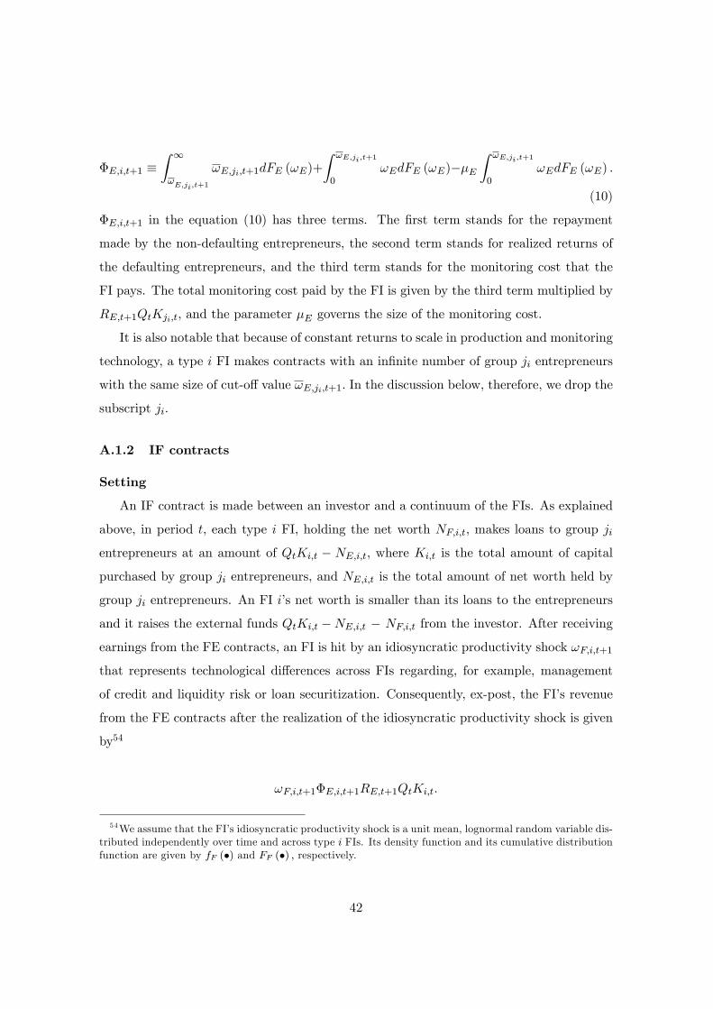
�E;i;t+1 �Z 1

!E;ji;t+1

!E;ji;t+1dFE (!E)+

Z !E;ji;t+1

0!EdFE (!E)��E

Z !E;ji;t+1

0!EdFE (!E) :

(10)

�E;i;t+1 in the equation (10) has three terms. The �rst term stands for the repayment

made by the non-defaulting entrepreneurs, the second term stands for realized returns of

the defaulting entrepreneurs, and the third term stands for the monitoring cost that the

FI pays. The total monitoring cost paid by the FI is given by the third term multiplied by

RE;t+1QtKji;t; and the parameter �E governs the size of the monitoring cost.

It is also notable that because of constant returns to scale in production and monitoring

technology, a type i FI makes contracts with an in�nite number of group ji entrepreneurs

with the same size of cut-o¤ value !E;ji;t+1: In the discussion below, therefore, we drop the

subscript ji:

A.1.2 IF contracts

Setting

An IF contract is made between an investor and a continuum of the FIs. As explained

above, in period t; each type i FI, holding the net worth NF;i;t; makes loans to group ji

entrepreneurs at an amount of QtKi;t � NE;i;t; where Ki;t is the total amount of capital

purchased by group ji entrepreneurs, and NE;i;t is the total amount of net worth held by

group ji entrepreneurs. An FI i�s net worth is smaller than its loans to the entrepreneurs

and it raises the external funds QtKi;t �NE;i;t � NF;i;t from the investor. After receiving

earnings from the FE contracts, an FI is hit by an idiosyncratic productivity shock !F;i;t+1

that represents technological di¤erences across FIs regarding, for example, management

of credit and liquidity risk or loan securitization. Consequently, ex-post, the FI�s revenue

from the FE contracts after the realization of the idiosyncratic productivity shock is given

by54

!F;i;t+1�E;i;t+1RE;t+1QtKi;t:

54We assume that the FI�s idiosyncratic productivity shock is a unit mean, lognormal random variable dis-tributed independently over time and across type i FIs. Its density function and its cumulative distributionfunction are given by fF (�) and FF (�) ; respectively.

42

There are informational asymmetries between the investor and the FI. The investor can

observe the realization of the idiosyncratic shock only if it pays the monitoring cost. Under

these circumstances, as with FE contracts, the IF contract speci�es:

� the amount of debt that a type i FI borrows from the investor, QtKi;t � NE;i;t �

NF;i;t; and

� the cut-o¤ value of idiosyncratic shock !F;i;t+1;which we denote by !F;i;t+1; such that

the FI repays its debt if !F;i;t+1 � !F;i;t+1 and declares a default if otherwise.

As a result of the IF contracts, a portion of the FIsR1!F;i;t+1

dFF (!F ) do not default,

while the remainder default. Ex-post, a default FI i receives nothing and a non-default FI

i receives the earnings shown below:

(!F;i;t+1 � !F;i;t+1) �E;i;t+1RE;t+1QtKi;t: (11)

The loan rate that is paid by a non-default FI i to an investor is therefore given by

rF;i;t+1 �!F;i;t+1�E;i;t+1RE;t+1QtKi;t

QtKi;t �NE;i;t �NF;i;t: (12)

Investor�s participation constraint

An investor participates in an IF contract only when the IF contract is more advanta-

geous. Denoting the risk-free rate in the economy by Rt; an investor�s net receipt from the

IF contracts must at least equal the return from a risk-free investment. That is for 8i;

�F;i;t+1�E;i;t+1RE;t+1QtKi;t � Rt [QtKi;t �NE;i;t �NF;i;t] ; (13)

where

�F;i;t+1 �Z 1

!F;i;t+1

!F;i;t+1dFF (!F ) +

Z !F;i;t+1

0!FdFF (!F )� �F

Z !F;i;t+1

0!FdFF (!F ) :

(14)

�F;i;t+1 has a similar structure to �E;i;t+1; as shown in the equation (10). In particular,

it is notable that the third term of �F;i;t+1 multiplied by the term �E;i;t+1RE;t+1QtKi;t

43

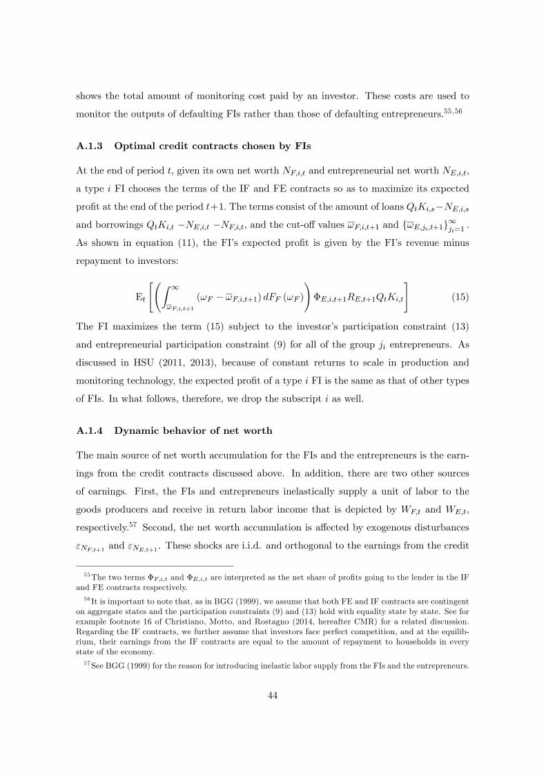
shows the total amount of monitoring cost paid by an investor. These costs are used to

monitor the outputs of defaulting FIs rather than those of defaulting entrepreneurs.55,56

A.1.3 Optimal credit contracts chosen by FIs

At the end of period t; given its own net worth NF;i;t and entrepreneurial net worth NE;i;t;

a type i FI chooses the terms of the IF and FE contracts so as to maximize its expected

pro�t at the end of the period t+1: The terms consist of the amount of loans QtKi;s�NE;i;s

and borrowings QtKi;t �NE;i;t �NF;i;t; and the cut-o¤ values !F;i;t+1 and f!E;ji;t+1g1ji=1

:

As shown in equation (11), the FI�s expected pro�t is given by the FI�s revenue minus

repayment to investors:

Et

" Z 1

!F;i;t+1

(!F � !F;i;t+1) dFF (!F )!�E;i;t+1RE;t+1QtKi;t

#(15)

The FI maximizes the term (15) subject to the investor�s participation constraint (13)

and entrepreneurial participation constraint (9) for all of the group ji entrepreneurs. As

discussed in HSU (2011, 2013), because of constant returns to scale in production and

monitoring technology, the expected pro�t of a type i FI is the same as that of other types

of FIs. In what follows, therefore, we drop the subscript i as well:

A.1.4 Dynamic behavior of net worth

The main source of net worth accumulation for the FIs and the entrepreneurs is the earn-

ings from the credit contracts discussed above. In addition, there are two other sources

of earnings. First, the FIs and entrepreneurs inelastically supply a unit of labor to the

goods producers and receive in return labor income that is depicted by WF;t and WE;t;

respectively.57 Second, the net worth accumulation is a¤ected by exogenous disturbances

"NF;t+1 and "NE;t+1 . These shocks are i.i.d. and orthogonal to the earnings from the credit

55The two terms �F;i;t and �E;i;t are interpreted as the net share of pro�ts going to the lender in the IFand FE contracts respectively.56 It is important to note that, as in BGG (1999), we assume that both FE and IF contracts are contingent

on aggregate states and the participation constraints (9) and (13) hold with equality state by state. See forexample footnote 16 of Christiano, Motto, and Rostagno (2014, hereafter CMR) for a related discussion.Regarding the IF contracts, we further assume that investors face perfect competition, and at the equilib-rium, their earnings from the IF contracts are equal to the amount of repayment to households in everystate of the economy.57See BGG (1999) for the reason for introducing inelastic labor supply from the FIs and the entrepreneurs.

44

contracts. The aggregate net worths of the FIs and the entrepreneurs then evolve according

to the equations below:

NF;t+1 = FVF;t+1 +WF;t

Pt+ "NF;t+1 ; and (16)

NE;t+1 = EVE;t+1 +WE;t

Pt+ "NE ;t+1; (17)

with

VF;t+1 � (1� �F (!F;t+1))�E (!E;t+1)RE;t+1QtKt; and

VE;t+1 � (1� �E (!E;t+1))RE;t+1QtKt;

where

�F (!F;t+1) �Z 1

!F;t+1

!F;t+1dFF (!F ) +

Z !F;t+1

0!FdFF (!F ) ; and

�E (!E;t+1) �Z 1

!E;t+1

!E;t+1dFE (!E) +

Z !E;t+1

0!EdFE (!E) :

58

Here, Pt denotes the nominal price of consumption goods. Note that we assume that FIs

and entrepreneurs survive into the next period with a probability F and E ; and those

who are in business in period t and fail to survive into period t+1 consume (1� E)VE;t+1and (1� F )VF;t+1 and exit from the economy.

A.2 Households

As described in the main text, there is a continuum of households indexed by h 2 [0; 1], and

each household is composed of Ht identical workers. Denoting total consumption and labor

inputs and the variables divided by the household�s size as Ct (h) ; L (h) ; c (h) ; and l (h) ;

respectively, the household�s expected utility Ut (h) is given by the following equation.

Ut (h) � Et

24 1Xq=0

�qdt+qHt+q

(ln (ct+q (h)� �hct+q�1 (h))� '

lt+q (h)1+v

1 + v

)35 ; (18)

45

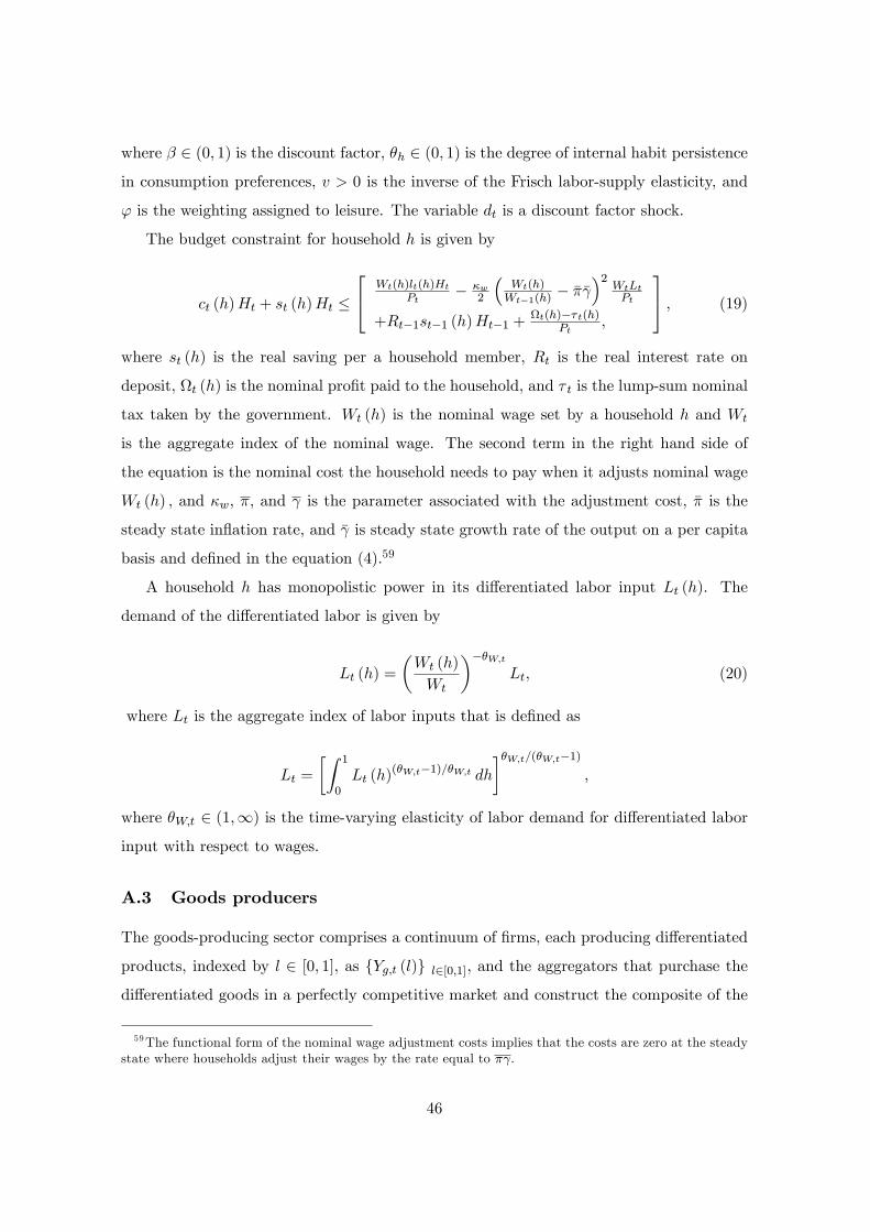
where � 2 (0; 1) is the discount factor, �h 2 (0; 1) is the degree of internal habit persistence

in consumption preferences, v > 0 is the inverse of the Frisch labor-supply elasticity, and

' is the weighting assigned to leisure. The variable dt is a discount factor shock.

The budget constraint for household h is given by

ct (h)Ht + st (h)Ht �

24 Wt(h)lt(h)HtPt

� �w2

�Wt(h)Wt�1(h)

� ��� �2

WtLtPt

+Rt�1st�1 (h)Ht�1 +t(h)�� t(h)

Pt;

35 ; (19)

where st (h) is the real saving per a household member, Rt is the real interest rate on

deposit, t (h) is the nominal pro�t paid to the household, and � t is the lump-sum nominal

tax taken by the government. Wt (h) is the nominal wage set by a household h and Wt

is the aggregate index of the nominal wage. The second term in the right hand side of

the equation is the nominal cost the household needs to pay when it adjusts nominal wage

Wt (h) ; and �w; �; and is the parameter associated with the adjustment cost, �� is the

steady state in�ation rate, and � is steady state growth rate of the output on a per capita

basis and de�ned in the equation (4).59

A household h has monopolistic power in its di¤erentiated labor input Lt (h). The

demand of the di¤erentiated labor is given by

Lt (h) =

�Wt (h)

Wt

���W;tLt; (20)

where Lt is the aggregate index of labor inputs that is de�ned as

Lt =

�Z 1

0Lt (h)

(�W;t�1)=�W;t dh

��W;t=(�W;t�1);

where �W;t 2 (1;1) is the time-varying elasticity of labor demand for di¤erentiated labor

input with respect to wages.

A.3 Goods producers

The goods-producing sector comprises a continuum of �rms, each producing di¤erentiated

products, indexed by l 2 [0; 1], as fYg;t (l)g l2[0;1]; and the aggregators that purchase the

di¤erentiated goods in a perfectly competitive market and construct the composite of the

59The functional form of the nominal wage adjustment costs implies that the costs are zero at the steadystate where households adjust their wages by the rate equal to � :

46

goods Yg;t .

Production function

The aggregators produce the composite of the di¤erentiated goods Yg;t by the technol-

ogy described below.

Yg;t =

�Z 1

0Yg;t (l)

(�PY ;t�1)=�PY ;t dl

��PY ;t=(�PY ;t�1);

where �PY ;t 2 (1;1) denotes the elasticity of substitution between di¤erentiated products.

Note also that the demand for each of the di¤erentiated products produced by �rm l is

derived from the optimization behavior of the aggregator and is represented by

Yg;t (l) =

�Pt (l)

Pt

���PY ;tYg;t; (21)

where fPt (l)g l2[0;1] is the nominal price of the di¤erentiated products. These prices are

related to the nominal price of the �nal goods by

Pt =

�Z 1

0Pt (l)

1��PY ;t dl

� 11��PY ;t

:

The production function of a di¤erentiated �rm l is given by

Yg;t (l) = Za;tAa;tt (l) [Lt (l)

�]1� h(Kt�1 (l)Ut (l))

1����E��FIi1�

� Ft (22)

Here, Za;t and Aa;t are a non-stationary and stationary component of neutral technology,

respectively, and Lt (l), Kt�1 (l), and Ut (l) are labor inputs, capital stock, and capacity

utilization rate of the capital stock in �rm l.60

60We assume that the capacity utilization rate Ut is determined by entrepreneurs, and a �rm l determinesonly the product Kt�1 (l)Ut (l) : We also assume that entrepreneurs need to pay the real cost of

�U�U�U+1t � 1

��U + 1

;

in choosing the capacity utilization rate of capital Ut. Here �U , �U are parameters. The real net return oncapital Kt�1 received by the entrepreneurs can then be expressed by the following equation.

RE;t =

Ut ~RE;tPt

��U

�U�U+1t �1

��U+1

+ (1� �)QtQt�1

:

where ~RE;t is the nominal gross return to capital inputs, Kt�1(l)Ut(l).

47

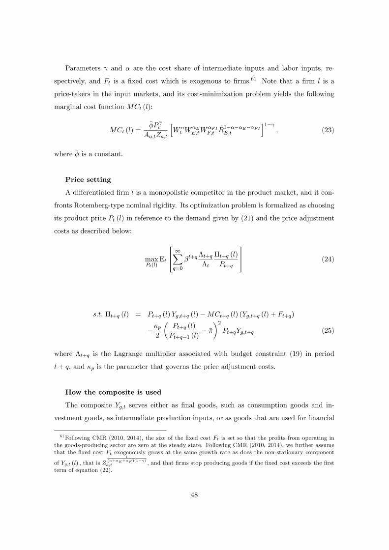
Parameters and � are the cost share of intermediate inputs and labor inputs, re-

spectively, and Ft is a �xed cost which is exogenous to �rms.61 Note that a �rm l is a

price-takers in the input markets, and its cost-minimization problem yields the following

marginal cost function MCt (l):

MCt (l) =��P t

Aa;tZa;t

hW�t W

�EE;tW

�FIF;t

~R1����E��FIE;t

i1� ; (23)

where �� is a constant.

Price setting

A di¤erentiated �rm l is a monopolistic competitor in the product market, and it con-

fronts Rotemberg-type nominal rigidity. Its optimization problem is formalized as choosing

its product price Pt (l) in reference to the demand given by (21) and the price adjustment

costs as described below:

maxPt(l)

Et

24 1Xq=0

�t+q�t+q�t

�t+q (l)

Pt+q

35 (24)

s:t: �t+q (l) = Pt+q (l)Yg;t+q (l)�MCt+q (l) (Yg;t+q (l) + Ft+q)

��p2

�Pt+q (l)

Pt+q�1 (l)� ��

�2Pt+qYg;t+q (25)

where �t+q is the Lagrange multiplier associated with budget constraint (19) in period

t+ q; and �p is the parameter that governs the price adjustment costs.

How the composite is used

The composite Yg;t serves either as �nal goods, such as consumption goods and in-

vestment goods, as intermediate production inputs, or as goods that are used for �nancial

61Following CMR (2010, 2014), the size of the �xed cost Ft is set so that the pro�ts from operating inthe goods-producing sector are zero at the steady state. Following CMR (2010, 2014), we further assumethat the �xed cost Ft exogenously grows at the same growth rate as does the non-stationary component

of Yg;t (l) ; that is Z1

(�+�E+�F )(1� )a;t , and that �rms stop producing goods if the �xed cost exceeds the �rst

term of equation (22).

48

intermediation activity, namely monitoring costs. The allocation of the gross output is

given by

Yg;t =

Final Outputz }| {Ct +

ItZd;tAd;t

+Gt +

Intermediate Inputsz }| {Z 1

0t (l) dl +

Inputs for Capacity Utilizationz }| {�U

�U U+1t � 1

��U + 1

Kt�1

+

Monitoring Costsz }| {��E

�Z !E;t

0!EdFE (!E)

�+ �F

�Z !F;t

0!FdFF (!F )

��RE;tQt�1Kt�1

+

Consumption by Exiting FIs and Entrepreneursz }| {(1� F )VF;t + (1� E)VE;t : (26)

where It is aggregate investment, Zd;t is a non-stationary component of investment-speci�c

technology, Ad;t is a stationary component of investment-speci�c technology, and Gt is

government expenditure.

A.4 Capital goods producer

Capital goods producers purchase �nal goods It= (Zd;tAd;t), convert them to capital goods

Kt with the technology FI;t; and sell the goods to the entrepreneurs at price Qt: Their

optimization problem is to maximize the pro�t shown below:

maxitEt

24 1Xq=0

�t+q�t+q�t

�Qt+q (Kt+q � (1� �)Kt+q�1)�

It+qZd;tAd;t

�35 :Note that the capital depreciates by the rate � in each period and evolves as follows:

Kt = (1� FI (It; It�1)) It + (1� �)Kt�1; (27)

where FI is de�ned as follows:

FI (It+q; It+q�1; ZI;t+q) ��I2

�It+qIt+q�1

ZI;t+q � ��� gZd;ss�2

:

Here, �I and ZI;t+q constitute the investment adjustment cost, and gZd;ss is the steady

state growth rate of investment-speci�c technology.

49

A.5 De�ning aggregate variables

As with CMR (2010), the real GDP Yt in the model is given as follows:

Yt = Ct +It

Zd;tAd;t+Gt; (28)

The CPI �t is de�ned by

�t =PtPt�1

: (29)

The real interest rate Rt is given by the Fisher equation that connects the nominal interest

rate Rn;t and the expected in�ation Et [�t+1]:

Rt =Rn;t

Et [�t+1]:

Also, for the purposes of the estimation exercise below, we de�ne the Solow residual as:

�t =Yt

(Lt) L (Kt�1)

1� L; (30)

where L is the steady state labor share of income.

A.6 Government sector

The government collects a per capita lump-sum tax � t from households to �nance gov-

ernment purchase PtGt whose amount is exogenously given: We assume that a balanced

budget is maintained in each period t as follows:

PtGt = � t

The central bank adjusts the policy rate according to the Taylor rule that is already

described in the equation (1) in the main text.

50

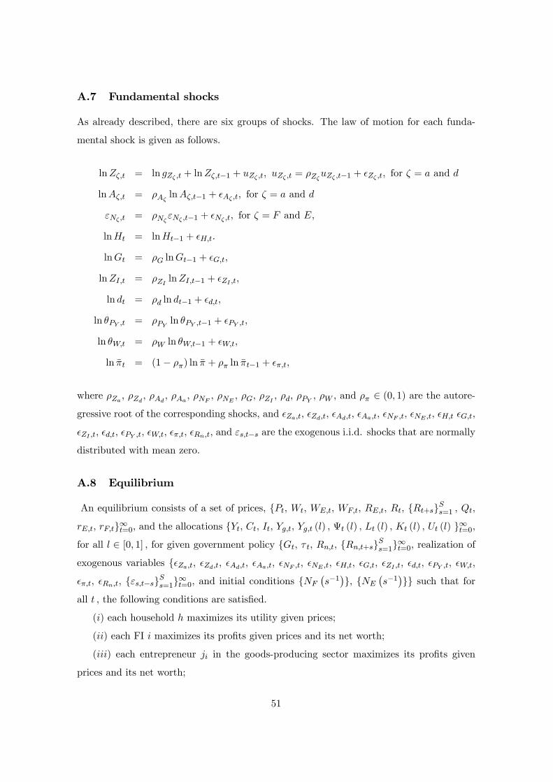
A.7 Fundamental shocks

As already described, there are six groups of shocks. The law of motion for each funda-

mental shock is given as follows.

lnZ�;t = ln gZ� ;t + lnZ�;t�1 + uZ� ;t; uZ� ;t = �Z�uZ� ;t�1 + �Z� ;t; for � = a and d

lnA�;t = �A� lnA�;t�1 + �A� ;t; for � = a and d

"N� ;t = �N�"N� ;t�1 + �N� ;t; for � = F and E;

lnHt = lnHt�1 + �H;t:

lnGt = �G lnGt�1 + �G;t;

lnZI;t = �ZI lnZI;t�1 + �ZI ;t;

ln dt = �d ln dt�1 + �d;t;

ln �PY ;t = �PY ln �PY ;t�1 + �PY ;t;

ln �W;t = �W ln �W;t�1 + �W;t;

ln ��t = (1� ��) ln �� + �� ln ��t�1 + ��;t;

where �Za ; �Zd ; �Ad ; �Aa ; �NF ; �NE ; �G; �ZI ; �d; �PY ; �W ; and �� 2 (0; 1) are the autore-

gressive root of the corresponding shocks, and �Za;t; �Zd;t; �Ad;t; �Aa;t; �NF ;t; �NE ;t; �H;t �G;t;

�ZI ;t; �d;t; �PY ;t; �W;t; ��;t; �Rn;t; and "s;t�s are the exogenous i.i.d. shocks that are normally

distributed with mean zero.

A.8 Equilibrium

An equilibrium consists of a set of prices, fPt; Wt; WE;t; WF;t; RE;t; Rt; fRt+sgSs=1 ; Qt;

rE;t; rF;tg1t=0, and the allocations fYt; Ct; It; Yg;t; Yg;t (l) ; t (l) ; Lt (l) ; Kt (l) ; Ut (l) g1t=0;

for all l 2 [0; 1] ; for given government policy fGt; � t; Rn;t; fRn;t+sgSs=1g1t=0, realization of

exogenous variables f�Za;t; �Zd;t; �Ad;t; �Aa;t; �NF ;t; �NE ;t; �H;t; �G;t; �ZI ;t; �d;t; �PY ;t; �W;t;

��;t; �Rn;t; f"s;t�sgSs=1g1t=0; and initial conditions fNF

�s�1�g; fNE

�s�1�gg such that for

all t ; the following conditions are satis�ed.

(i) each household h maximizes its utility given prices;

(ii) each FI i maximizes its pro�ts given prices and its net worth;

(iii) each entrepreneur ji in the goods-producing sector maximizes its pro�ts given

prices and its net worth;

51

(iv) each goods producer l in the goods-producing sector maximizes its pro�ts given

prices;

(v) each capital goods producer in the goods-producing sector maximizes its pro�ts

given prices;

(vi) the government budget constraint holds;

(vii) the central bank sets the policy rate following the Taylor rule; and

(viii) markets clear.

52

B Estimation

B.1 Estimation strategy

We �rst detrend the model variables by dividing them by the stochastic trend. We trend

the real variables other than the capital stock Kt, such as output Yt and the net worth

Nt; with the term expressed by the function of the steady-state growth rate of the two

technologies and that of the working-age population, Z1

(1� )(�+�E+�F )a;t Z

(1����E��F )�+�E+�F

d;t Ht; and

detrend the capital stock Kt; with the term Z1

(1� )(�+�E+�F )a;t Z

1�+�E+�Fd;t Ht. We then con-

duct a Bayesian estimation following existing studies such as CMR (2014). We �rst write

the model�s equilibrium conditions in a state-space representation and derive the likeli-

hood function of the system of equilibrium conditions using the Kalman �lter. We then

combine the likelihood function with the priors for the parameters to obtain the posterior

density function numerically. In this process, we use the random walk Metropolis-Hastings

algorithm.

B.2 Calibration, Prior Distribution, and Posterior Distribution

Calibrated parameters

Some parameter values are calibrated following existing studies. These include the

discount factor �; the elasticity of substitution between di¤erentiated products �PY ; the

elasticity of substitution between di¤erentiated labor inputs �W ; the depreciation rate of

the capital stock �; the share of the intermediate input, labor input, entrepreneurial labor

input and the FI labor input in goods production ; �; �E and �F ; and the utility weight

on leisure ': Values for and � are constructed using the historical average of intermediate

goods usage divided by gross output, both of which are reported in an input-output table,

and the compensation of employees divided by GDP in SNA, respectively. In addition, we

set �U so that the utilization rate of capital stock is unity at the steady state. See Table 1

for the values of these parameters.

Estimated parameters

We estimate the remaining parameters. See Table 2 for the values of these parameters.

The type, mean, and standard deviation of the prior distribution are mostly taken from

53

existing studies such as Edge et al. (2008). They are given in the �rst to the third columns.

In estimating the six parameters that are related to the IF and FE contracts, that include

two parameters that govern monitoring costs �F and �E ; variance of idiosyncratic shocks

to borrowers �F and �E ; and survival rates F and E ; we follow HSU (2011) and set the

prior mean of these parameters so that they satisfy the six equilibrium conditions stated

below at the steady state: (1) the annualized spread between the FIs�borrowing rate and

the risk-free rate rF � R is 56 bps; (2) the ratio of net worth held by FIs to aggregate

capital stock NF = (QK) is 0.1; (3) the ratio of net worth held by the entrepreneurs in

the goods-producing sector to aggregate capital stock NE= (QK) is 0.6; (4) the annualized

failure rate of the FIs is 1%; (5) the annualized failure rate of the entrepreneurs in the

goods-producing sector is 1%; and (6) the annualized spread between the FI loan rate

and the FI borrowing rate rE � rF ; equals 442 bps. Except for conditions (4) and (5),

the conditions above are chosen so that they are consistent with the historical average of

Japanese data.62 We borrow condition (5) from BGG (1999) and assume that the same

condition holds in the FI sector as well. This can be seen in condition (4).

Posterior distribution

To calculate the posterior distribution and to evaluate the marginal likelihood of the

model, we employ the Metropolis-Hastings algorithm. To do this, we create a sample of

400,000 draws, disregarding the initial 200,000 draws. Estimated posterior distributions

of parameters are also shown in Table 2. The last three columns of the table display the

posterior mean and the con�dence intervals for the estimated parameters.

62We take the numbers for conditions (2) and (3) from the Flow of Funds Accounts. We use the long-termprime lending rate and the deposit rate adopted by the Bank of Japan to obtain conditions (1) and (6),respectively.

54

Table 1: Calibrated Parameters

Values of calibrated parameters

Labor share (household) 0.6

Labor share (entrepreneur) 0.02

Labor share (FI) 0.02

Share of intermediate goods 0.583

Scaling parameter of capital utilization adjustment cost 0.05

Weight on labor disutility 0.2

Households’ discount factor (quarterly) 0.998

Capital depreciation rate (quarterly) 0.028

Elasticity of substitution between differentiated products at the steady state 7

Elasticity of substitution between differentiated labor inputs at the steady state 7

E

FI

U

YP

W

Table 2: Estimated Parameters

Values of estimated parameters (prior and posterior distributions)

Distribution Mean S.D. Mean 5th percentiles 95th percentilesElasticity of labor supply gamma 0.8 0.075 0.887 0.763 1.011Capital stock adjustment cost gamma 2 0.25 2.275 1.889 2.649Price adjustment cost gamma 12 1 6.950 6.690 7.298Nominal wage adjustment cost gamma 2.5 0.5 0.887 0.579 1.184Policy weight on inflation in Taylor rule normal 2.75 0.05 2.867 2.784 2.946Monetary policy smoothing beta 0.5 0.01 0.514 0.498 0.531Inverse elasticity of capital utilization rate gamma 5 1 5.888 4.886 7.139Riskiness of idiosyncratic productivities (FIs) gamma 0.104 0.002 0.102 0.099 0.106Riskiness of idiosyncratic productivities (entrepreneurs) gamma 0.309 0.002 0.309 0.306 0.313Monitoring cost (IF contract) gamma 0.539 0.01 0.535 0.519 0.552Monitoring cost (FE contract) gamma 0.02 0.01 0.038 0.017 0.060Survival rates (FIs) beta 0.86 0.001 0.861 0.859 0.862Survival rates (entrepreneurs) beta 0.96 0.001 0.959 0.958 0.961Steady state value of technology (neutral) gamma 1.001 0.001 1.000 1.000 1.001Steady state value of technology (investment-specific) gamma 1.002 0.001 1.000 1.000 1.001Steady state value of target inflation rate normal 1.002 0.001 1.001 1.000 1.002Degree of internal habit persistence beta 0.6 0.15 0.136 0.052 0.219

Non-stationary technology shock (neutral) AR beta 0.5 0.15 0.145 0.052 0.228Stationary technology shock (neutral) AR beta 0.5 0.15 0.867 0.818 0.917Non-stationary technology shock (investment-specific) AR beta 0.5 0.15 0.517 0.365 0.676Stationary technology shock (investment-specific) AR beta 0.5 0.15 0.745 0.631 0.856Net worth shock (FIs) AR beta 0.5 0.15 0.194 0.075 0.311Net worth shock (entrepreneurs) AR beta 0.5 0.15 0.750 0.612 0.875External demand shock AR beta 0.5 0.15 0.961 0.939 0.987Investment adjustment shock AR beta 0.5 0.15 0.217 0.104 0.322Price markup shock AR beta 0.5 0.15 0.802 0.728 0.873Nominal wage markup shock AR beta 0.5 0.15 0.810 0.697 0.927Discount factor shock AR beta 0.5 0.15 0.765 0.638 0.908Target inflation rate shock AR beta 0.5 0.15 0.450 0.394 0.505

Non-stationary technology shock (neutral) SD invg 0.01 5 0.002 0.002 0.003Stationary technology shock (neutral) SD invg 0.05 5 0.006 0.006 0.006Non-stationary technology shock (investment-specific) SD invg 0.01 5 0.002 0.002 0.003Stationary technology shock (investment-specific) SD invg 0.05 5 0.006 0.006 0.006Monetary policy shock SD invg 0.01 5 0.002 0.002 0.002Net worth shock (FIs) SD invg 0.02 5 0.003 0.003 0.004Net worth shock (entrepreneurs) SD invg 0.02 5 0.005 0.003 0.006External demand shock SD invg 0.01 5 0.071 0.058 0.084Investment adjustment shock SD invg 0.01 5 0.031 0.026 0.036Price markup shock SD invg 0.01 5 0.029 0.025 0.032Nominal wage markup shock SD invg 0.01 5 0.094 0.067 0.120Discount factor shock SD invg 0.015 5 0.005 0.003 0.006Target inflation rate shock SD invg 0.01 5 0.004 0.003 0.0041Q ahead anticipated monetary policy shock SD invg 0.01 5 0.001 0.001 0.0012Q ahead anticipated monetary policy shock SD invg 0.01 5 0.001 0.001 0.0013Q ahead anticipated monetary policy shock SD invg 0.01 5 0.001 0.001 0.0014Q ahead anticipated monetary policy shock SD invg 0.01 5 0.001 0.001 0.0015Q ahead anticipated monetary policy shock SD invg 0.01 5 0.001 0.001 0.0016Q ahead anticipated monetary policy shock SD invg 0.01 5 0.001 0.001 0.0017Q ahead anticipated monetary policy shock SD invg 0.01 5 0.001 0.001 0.0018Q ahead anticipated monetary policy shock SD invg 0.01 5 0.001 0.001 0.0019Q ahead anticipated monetary policy shock SD invg 0.01 5 0.001 0.001 0.00110Q ahead anticipated monetary policy shock SD invg 0.01 5 0.001 0.001 0.00111Q ahead anticipated monetary policy shock SD invg 0.01 5 0.001 0.001 0.00112Q ahead anticipated monetary policy shock SD invg 0.01 5 0.001 0.001 0.001

Prior distribution Posterior distribution

(1) Decomposition of the natural rate decline

(2) Variance decomposition of the natural rate

Notes: 1. In (2), we first compute the sum of squares for the contribution of each factors to variations in the natural rate over theNotes: 1. sample period. We then divide the sum of squares for each factor by the sum of the factors.Notes: 2. Contribution of neutral technology is the sum of the contribution of both non-stationary and stationary shocks.Notes: 3. Contribution of financial factors is the sum of the contribution of net worth shocks to the FIs and that to entrepreneurs.Notes: 4. Contribution of investment-specific technology is the sum of the contribution of both non-stationary and stationary shocks.Notes: 5. Contribution of demand factors is the sum of the contribution of shocks to the external demand and discount factor.

Table 3: Determinants of the Natural Rate

(%)

Neutral technology 58.1

Financial factors 24.0

Working-age population 3.8

Investment-specifictechnology

4.3

Demand factors 7.9

Others 1.9

4.15 0.31 3.84

Neutral technology 1.58 -0.57 2.16

Financial factors -0.49 0.92 -1.40

Working-age population 0.29 -0.40 0.69

Investment-specifictechnology

0.14 -0.34 0.48

Demand factors 0.54 -0.04 0.58

Changes(i) － (ii)

(% points)

(i) 1980s(%)

(ii) 2013-2017(%)

Natural rate

(1) Decomposition of the expected natural rate decline

(2) Variance decomposition of the natural rate and the expected natural rate

Notes: 1. In (1), the expected natural rate is the average of expected natural rates from the current period to 10 years ahead.Notes: 2. In (2), we first compute the sum of squares for the contribution of each factors to variations in the natural rate andNotes: 2. expected natural rates over 1 year, 5 year, and 10 year horizons, respectively, over the sample period. We then divideNotes: 2. the sum of squares for each factor by the sum of the factors.Notes: 3. Contribution of neutral technology is the sum of the contribution of both non-stationary and stationary shocks.Notes: 4. Contribution of financial factors is the sum of the contribution of net worth shocks to the FIs and that to entrepreneurs.Notes: 5. Contribution of investment-specific technology is the sum of the contribution of both non-stationary and stationary shocks.Notes: 6. Contribution of demand factors is the sum of the contribution of shocks to the external demand and discount factor.

Table 4: Determinants of the Expected Natural Rate

1 year(%)

5 year(%)

10 year(%)

Neutral technology 58.1 52.4 54.7 57.1

Financial factors 24.0 27.8 15.9 10.1

Working-age population 3.8 4.9 6.3 6.2

Investment-specifictechnology

4.3 5.0 11.4 12.5

Demand factors 7.9 8.5 11.4 14.0

Others 1.9 1.4 0.2 0.1

Natural rate(%)

Expected natural rate

2.56 0.49 2.07

Neutral technology 0.77 -0.11 0.87

Financial factors -0.07 0.19 -0.26

Working-age population 0.13 -0.18 0.32

Investment-specifictechnology

0.22 -0.22 0.44

Demand factors 0.26 0.02 0.23

Changes(i) － (ii)

(% points)

Expected natural rate

(i) 1980s(%)

(ii) 2013-2017(%)

(1) Decomposition of the natural rate and expected natural rate declines

(2) Variance decomposition of the natural rate and expected natural rate

Notes: 1. Figures indicate the range of estimates by various specifications, and those in brackets are values under the baselineNotes: 1. model.Notes: 2. In (1), the expected natural rate is the average of expected natural rates from the current period to 10 years ahead.Notes: 3. In (2), we first compute the sum of squares for the contribution of each factors to variations in the natural rate andNotes: 2. expected natural rates over 10 year horizons, over the sample period. We then divide the sum of squares for each factorNotes: 2. by the sum of the factors.Notes: 4. Contribution of neutral technology is the sum of the contribution of both non-stationary and stationary shocks.Notes: 5. Contribution of financial factors is the sum of the contribution of net worth shocks to the FIs and that to entrepreneurs.Notes: 6. Contribution of investment-specific technology is the sum of the contribution of both non-stationary and stationary shocks.Notes: 7. Contribution of demand factors is the sum of the contribution of shocks to the external demand and discount factor.

Table 5: Robustness Check (1) : Anticipated Shocks

Changes from 1980s to 2013-2017 (% points)

2.14 ～ 2.22　[ 2.07 ]

0.20 ～ 0.25　[ 0.23 ]

0.40 ～ 0.45　[ 0.44 ]

0.31 ～ 0.32　[ 0.32 ]

-0.24 ～ -0.17　[ -0.26 ]

0.82 ～ 1.02　[ 0.87 ]

1.71 ～ 1.97　[ 2.16 ]

3.54 ～ 3.82　[ 3.84 ]

0.72 ～ 0.78　[ 0.58 ]

0.49 ～ 0.50　[ 0.48 ]

0.70　[ 0.69 ]

-1.44 ～ -1.08　[ -1.40 ]

Demand factors

Working-age population

Investment-specific technology

Demand factors

Natural rate

Neutral technology

Financial factors

Expected natural rate

Neutral technology

Financial factors

Working-age population

Investment-specific technology

Natural rate (%) Expected natural rate (%)47.9 ～ 56.5 61.1 ～ 62.6

[ 58.1 ] [ 57.1 ]12.1 ～ 26.9 2.8 ～ 6.5

[ 24.0 ] [ 10.1 ]3.7 ～ 4.7 5.2 ～ 5.7

[ 3.8 ] [ 6.2 ]3.9 ～ 4.6 10.6 ～ 11.1

[ 4.3 ] [ 12.5 ]13.2 14.9 ～ 18.3[ 7.9 ] [ 14.0 ]

3.0 ～ 10.6 0.2 ～ 1.0[ 1.9 ] [ 0.1 ]

Investment-specific technology

Demand factors

Others

Working-age population

Neutral technology

Financial factors

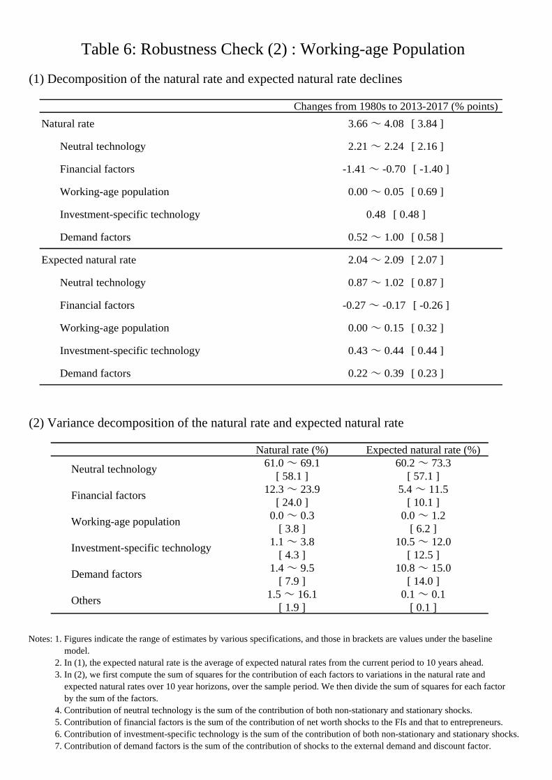
(1) Decomposition of the natural rate and expected natural rate declines

(2) Variance decomposition of the natural rate and expected natural rate

Notes: 1. Figures indicate the range of estimates by various specifications, and those in brackets are values under the baselineNotes: 1. model.Notes: 2. In (1), the expected natural rate is the average of expected natural rates from the current period to 10 years ahead.Notes: 3. In (2), we first compute the sum of squares for the contribution of each factors to variations in the natural rate andNotes: 2. expected natural rates over 10 year horizons, over the sample period. We then divide the sum of squares for each factorNotes: 2. by the sum of the factors.Notes: 4. Contribution of neutral technology is the sum of the contribution of both non-stationary and stationary shocks.Notes: 5. Contribution of financial factors is the sum of the contribution of net worth shocks to the FIs and that to entrepreneurs.Notes: 6. Contribution of investment-specific technology is the sum of the contribution of both non-stationary and stationary shocks.Notes: 7. Contribution of demand factors is the sum of the contribution of shocks to the external demand and discount factor.

Table 6: Robustness Check (2) : Working-age Population

Changes from 1980s to 2013-2017 (% points)

3.66 ～ 4.08　[ 3.84 ]

0.22 ～ 0.39　[ 0.23 ]

0.43 ～ 0.44　[ 0.44 ]

0.00 ～ 0.15　[ 0.32 ]

-0.27 ～ -0.17　[ -0.26 ]

0.87 ～ 1.02　[ 0.87 ]

2.04 ～ 2.09　[ 2.07 ]

0.52 ～ 1.00　[ 0.58 ]

0.48　[ 0.48 ]

0.00 ～ 0.05　[ 0.69 ]

-1.41 ～ -0.70　[ -1.40 ]

2.21 ～ 2.24　[ 2.16 ]

Demand factors

Working-age population

Investment-specific technology

Demand factors

Natural rate

Neutral technology

Financial factors

Expected natural rate

Neutral technology

Financial factors

Working-age population

Investment-specific technology

Natural rate (%) Expected natural rate (%)61.0 ～ 69.1 60.2 ～ 73.3

[ 58.1 ] [ 57.1 ]12.3 ～ 23.9 5.4 ～ 11.5

[ 24.0 ] [ 10.1 ]0.0 ～ 0.3 0.0 ～ 1.2

[ 3.8 ] [ 6.2 ]1.1 ～ 3.8 10.5 ～ 12.0

[ 4.3 ] [ 12.5 ]1.4 ～ 9.5 10.8 ～ 15.0

[ 7.9 ] [ 14.0 ]1.5 ～ 16.1 0.1 ～ 0.1

[ 1.9 ] [ 0.1 ]

Investment-specific technology

Demand factors

Others

Working-age population

Neutral technology

Financial factors

Figure 1: Outline of the Model

Raise funds throughIF contracts

Supply funds throughFE contracts

Rental cost

Capital stock

Consumptiongoods

Labor input

Monetary policy andgovernment policy

Central bankGovernment

Goodsprice

Wage

Capital goodsCapital goodsprice Intermediate goods

Capital goods producer

Supply fund to FIsthrough IF contracts

Deposit

Repayment

Financialintermediaries

Entrepreneurs

RepaymentLending

Household

Goods producers

Investment goods

Investment goods price

Goods-Producing Sector

Investors

RepaymentLending

(1) Real GDP (2) Real investment

(3) GDP deflator (4) Investment deflator

(5) Nominal wage (6) Working hours

Notes: 1. Series (1), (2), and (6) are on a per capita basis. For all variables, we use a quarter-on-quarter % change of the variableNotes: 1. rather than a year-on-year % change.Notes: 2. The shaded areas show the period of banking crisis based on the dating by Reinhart and Rogoff (2011) and the recessionNotes: 2. in the 14th business cycle in Japan based on the dating by the Cabinet Office.Sources: Cabinet Office, "National Accounts"; Ministry of Health, Labour and Welfare, "Monthly Labour Survey"; Ministry ofSources: Internal Affairs and Communications, "Labour Force Survey"; Reinhart and Rogoff (2011).

Figure 2: Data Used for Estimation (1)

-10

-5

0

5

10

81 85 90 95 00 05 10 15

y/y % chg.

CY-20

-10

0

10

20

30

81 85 90 95 00 05 10 15

y/y % chg.

CY

-4

-2

0

2

4

6

81 85 90 95 00 05 10 15

y/y % chg.

CY-6

-4

-2

0

2

4

6

81 85 90 95 00 05 10 15

y/y % chg.

CY

-8

-4

0

4

8

12

81 85 90 95 00 05 10 15

y/y % chg.

CY-6

-4

-2

0

2

4

81 85 90 95 00 05 10 15

y/y % chg.

CY

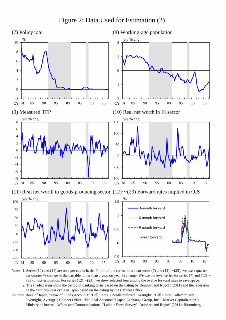
(7) Policy rate (8) Working-age population

(9) Measured TFP (10) Real net worth in FI sector

(11) Real net worth in goods-producing sector (12)～(23) Forward rates implied in OIS

Notes: 1. Series (10) and (11) are on a per capita basis. For all of the series other than series (7) and (12) ～(23), we use a quarter-Notes: 1. on-quarter % change of the variable rather than a year-on-year % change. We use the level series for series (7) and (12)～Notes: 1. (23) in our estimation. For series (12)～(23), we show selected four among the twelve forward rates to save space.Notes: 2. The shaded areas show the period of banking crisis based on the dating by Reinhart and Rogoff (2011) and the recessionNotes: 2. in the 14th business cycle in Japan based on the dating by the Cabinet Office.Sources: Bank of Japan, "Flow of Funds Accounts" "Call Rates, Uncollateralized Overnight" "Call Rates, CollateralizedSources: Overnight, Average"; Cabinet Office, "National Accounts"; Japan Exchange Group, Inc., "Market Capitalization";Sources: Ministry of Internal Affairs and Communications, "Labour Force Survey"; Reinhart and Rogoff (2011); Bloomberg.

Figure 2: Data Used for Estimation (2)

-0.5

0

0.5

1

1.5

81 85 90 95 00 05 10 15

3-month forward

6-month forward

9-month forward

1-year forward

%

CY

-2

0

2

4

6

8

10

81 85 90 95 00 05 10 15

%

CY-2

-1

0

1

2

81 85 90 95 00 05 10 15

y/y % chg.

CY

-8

-6

-4

-2

0

2

4

6

8

81 85 90 95 00 05 10 15

y/y % chg.

CY-100

-50

0

50

100

150

81 85 90 95 00 05 10 15

y/y % chg.

CY

-75

-50

-25

0

25

50

75

100

81 85 90 95 00 05 10 15

y/y % chg.

CY

Notes: 1. Figures for the natural rate in the baseline model are the moving average of the point estimate, and the shaded areasNotes: 2. are the 90% confidence intervals of the estimate.Notes: 2. Figures for the natural rate estimated based on Imakubo et al. (2015) are those for 1-year yield.Notes: 3. Figures for the potential growth rate are those released by the Research and Statistics Department of the Bank of Japan.

Sources: Bank of Japan; Bloomberg; Cabinet Office; Consensus Economics Inc., "Consensus Forecasts"; Imakubo et al. (2015);Sources: Laubach and Williams (2003); Reinhart and Rogoff (2011).

Figure 3: Estimated Level of Natural Rate

-3

-2

-1

0

1

2

3

4

5

6

7

80 82 84 86 88 90 92 94 96 98 00 02 04 06 08 10 12 14 16

R* in the baseline model

R* estimated based on Laubach and Williams (2003)

R* estimated based on Imakubo et al. (2015)

Potential growth rate

The period of banking crisis defined by Reinhart and

Rogoff (2011)

%

CY

Recession period inJapan that cametogether with theglobal financial crisis.

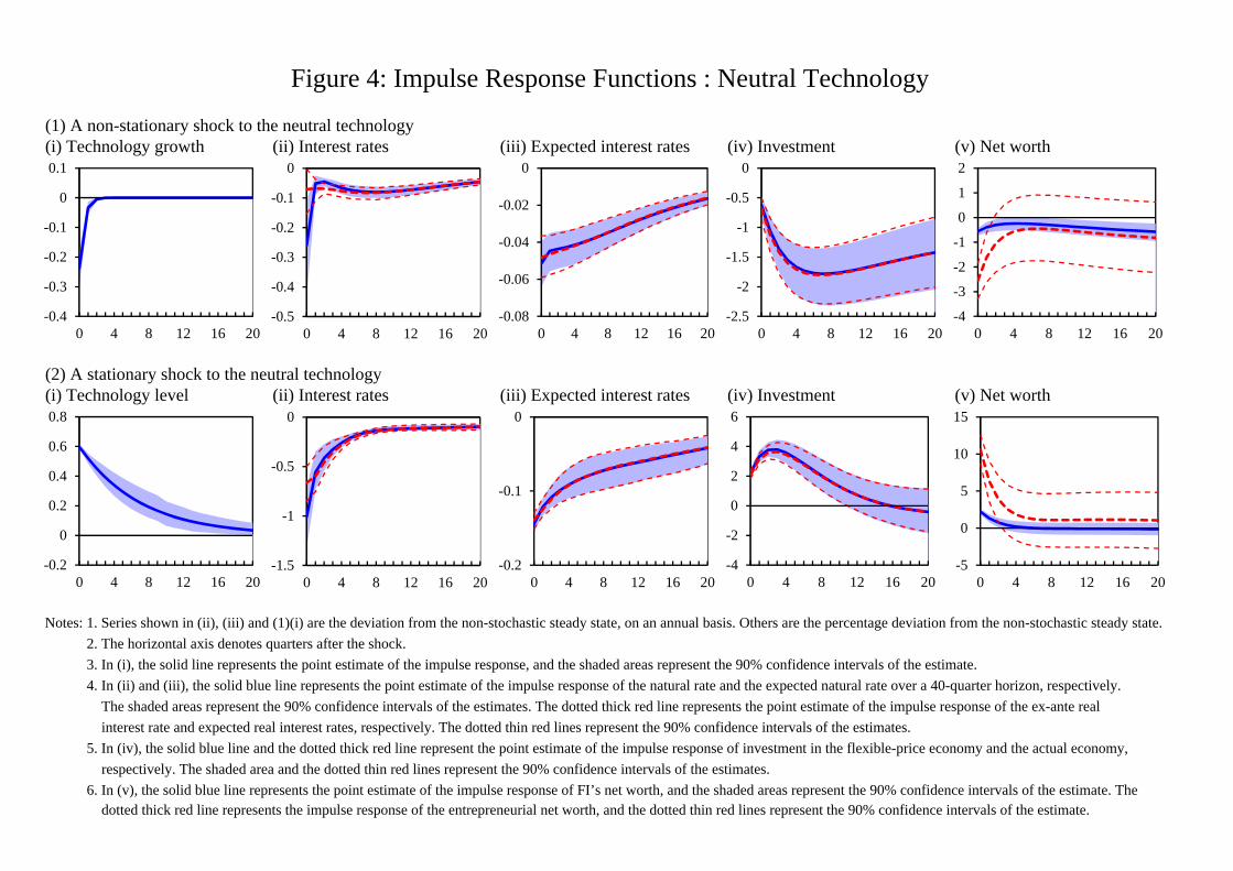
(1) A non-stationary shock to the neutral technology(i) Technology growth (ii) Interest rates (iii) Expected interest rates (iv) Investment (v) Net worth

(2) A stationary shock to the neutral technology(i) Technology level (ii) Interest rates (iii) Expected interest rates (iv) Investment (v) Net worth

Notes: 1. Series shown in (ii), (iii) and (1)(i) are the deviation from the non-stochastic steady state, on an annual basis. Others are the percentage deviation from the non-stochastic steady state.

Notes: 2. The horizontal axis denotes quarters after the shock.

Notes: 3. In (i), the solid line represents the point estimate of the impulse response, and the shaded areas represent the 90% confidence intervals of the estimate.

Notes: 4. In (ii) and (iii), the solid blue line represents the point estimate of the impulse response of the natural rate and the expected natural rate over a 40-quarter horizon, respectively.

Notes: 3. The shaded areas represent the 90% confidence intervals of the estimates. The dotted thick red line represents the point estimate of the impulse response of the ex-ante real

Notes: 3. interest rate and expected real interest rates, respectively. The dotted thin red lines represent the 90% confidence intervals of the estimates.

Notes: 5. In (iv), the solid blue line and the dotted thick red line represent the point estimate of the impulse response of investment in the flexible-price economy and the actual economy,

Notes: 4. respectively. The shaded area and the dotted thin red lines represent the 90% confidence intervals of the estimates.

Notes: 6. In (v), the solid blue line represents the point estimate of the impulse response of FI’s net worth, and the shaded areas represent the 90% confidence intervals of the estimate. TheNotes: 3. dotted thick red line represents the impulse response of the entrepreneurial net worth, and the dotted thin red lines represent the 90% confidence intervals of the estimate.

Figure 4: Impulse Response Functions : Neutral Technology

-0.5

-0.4

-0.3

-0.2

-0.1

0

0 4 8 12 16 20-4

-3

-2

-1

0

1

2

0 4 8 12 16 20-0.08

-0.06

-0.04

-0.02

0

0 4 8 12 16 20-0.4

-0.3

-0.2

-0.1

0

0.1

0 4 8 12 16 20-2.5

-2

-1.5

-1

-0.5

0

0 4 8 12 16 20

-1.5

-1

-0.5

0

0 4 8 12 16 20-5

0

5

10

15

0 4 8 12 16 20-0.2

-0.1

0

0 4 8 12 16 20-0.2

0

0.2

0.4

0.6

0.8

0 4 8 12 16 20-4

-2

0

2

4

6

0 4 8 12 16 20

(1) A shock to the FI’s net worth(i) Net worth (FIs) (ii) Interest rates (iii) Expected interest rates (iv) Investment (v) Net worth (Entrepreneurs)

(2) A shock to the Entrepreneurs’ net worth(i) Net worth (Entrepreneurs) (ii) Interest rates (iii) Expected interest rates (iv) Investment (v) Net worth (FIs)

Notes: 1. Series shown in (ii) and (iii) are the deviation from the non-stochastic steady state, on an annual basis. Others are the percentage deviation from the non-stochastic steady state.Notes: 2. The horizontal axis denotes quarters after the shock.Notes: 3. In (i) and (v), the solid line represents the point estimate of the impulse response, and the shaded areas represent the 90% confidence intervals of the estimate.Notes: 4. In (ii) and (iii), the solid blue line represents the point estimate of the impulse response of the natural rate and the expected natural rate over a 40-quarter horizon, respectively.Notes: 3. The shaded areas represent the 90% confidence intervals of the estimates. The dotted thick red line represents the point estimate of the impulse response of the ex-ante realNotes: 3. interest rate and expected real interest rates, respectively. The dotted thin red lines represent the 90% confidence intervals of the estimates.Notes: 5. In (iv), the solid blue line and the dotted thick red line represent the point estimate of the impulse response of investment in the flexible-price economy and the actual economy,Notes: 4. respectively. The shaded area and the dotted thin red lines represent the 90% confidence intervals of the estimates.

Figure 5: Impulse Response Functions : Financial Factors

-1.5

-1

-0.5

0

0.5

1

0 4 8 12 16 20-0.4

-0.3

-0.2

-0.1

0

0.1

0 4 8 12 16 20-0.06

-0.04

-0.02

0

0.02

0 4 8 12 16 20-8

-6

-4

-2

0

2

4

0 4 8 12 16 20-1.5

-1

-0.5

0

0.5

1

0 4 8 12 16 20

-0.4

-0.3

-0.2

-0.1

0

0 4 8 12 16 20-0.08

-0.06

-0.04

-0.02

0

0.02

0 4 8 12 16 20-6

-4

-2

0

2

4

6

0 4 8 12 16 20-8

-6

-4

-2

0

0 4 8 12 16 20-4

-3

-2

-1

0

1

0 4 8 12 16 20

(1) A shock to the working-age population (i) Population growth (ii) Interest rates (iii) Expected interest rates (iv) Investment (v) Net worth

(2) A non-stationary shock to the investment-specific technology(i) Technology growth (ii) Interest rates (iii) Expected interest rates (iv) Investment (v) Net worth

(3) A stationary shock to the investment-specific technology(i) Technology level (ii) Interest rates (iii) Expected interest rates (iv) Investment (v) Net worth

Notes: 1. Series shown in (ii), (iii), (1)(i) and (2)(i) are the deviation from the non-stochastic steady state, on an annual basis. Others are the percentage deviation from the non-stochasticNotes: 1. steady state.Notes: 2. See footnotes to Figure 4 for the explanation of each line and shaded area.

Figure 6: Impulse Response Functions : Working-age Population and Investment-specific Technology

-0.3

-0.2

-0.1

0

0.1

0 4 8 12 16 20-0.2

0

0.2

0.4

0.6

0.8

0 4 8 12 16 20-0.04

-0.02

0

0.02

0.04

0 4 8 12 16 20-2

-1

0

1

2

0 4 8 12 16 20

-1

-0.5

0

0.5

1

1.5

0 4 8 12 16 20

-0.4

-0.3

-0.2

-0.1

0

0.1

0 4 8 12 16 20-0.1

0

0.1

0.2

0.3

0 4 8 12 16 200

0.01

0.02

0.03

0.04

0 4 8 12 16 20-3

-2

-1

0

1

2

0 4 8 12 16 20

0

0.5

1

1.5

2

0 4 8 12 16 20

-0.001

-0.0008

-0.0006

-0.0004

-0.0002

0

0 4 8 12 16 20-0.0003

-0.0002

-0.0001

0

0 4 8 12 16 20-0.006

-0.004

-0.002

0

0.002

0 4 8 12 16 20

-0.003

-0.002

-0.001

0

0.001

0 4 8 12 16 20-0.004

-0.003

-0.002

-0.001

0

0 4 8 12 16 20

(1) A shock to the discount factor(i) Discount factor (ii) Interest rates (iii) Expected interest rates (iv) Investment (v) Net worth

(2) A shock to the external demand(i) External demand (ii) Interest rates (iii) Expected interest rates (iv) Investment (v) Net worth

Notes: 1. Series shown in (ii), and (iii) are the deviation from the non-stochastic steady state, on an annual basis. Others are the percentage deviation from the non-stochastic steady state.Notes: 2. The horizontal axis denotes quarters after the shock.Notes: 3. In (i), the solid line represents the point estimate of the impulse response, and the shaded areas represent the 90% confidence intervals of the estimate.Notes: 4. In (ii) and (iii), the solid blue line represents the point estimate of the impulse response of the natural rate and the expected natural rate over a 40-quarter horizon, respectively.Notes: 3. The shaded areas represent the 90% confidence intervals of the estimates. The dotted thick red line represents the point estimate of the impulse response of the ex-ante realNotes: 3. interest rate and expected real interest rates, respectively. The dotted thin red lines represent the 90% confidence intervals of the estimates.Notes: 5. In (iv), the solid blue line and the dotted thick red line represent the point estimate of the impulse response of investment in the flexible-price economy and the actual economy,Notes: 4. respectively. The shaded area and the dotted thin red lines represent the 90% confidence intervals of the estimates.Notes: 6. In (v), the solid blue line represents the point estimate of the impulse response of FI’s net worth, and the shaded areas represent the 90% confidence intervals of the estimate. TheNotes: 3. dotted thick red line represents the impulse response of the entrepreneurial net worth, and the dotted thin red lines represent the 90% confidence intervals of the estimate.

Figure 7: Impulse Response Functions : Demand Factors

-0.3

-0.2

-0.1

0

0 4 8 12 16 20-2.5

-2

-1.5

-1

-0.5

0

0 4 8 12 16 20-0.08

-0.06

-0.04

-0.02

0

0 4 8 12 16 20-2

-1

0

1

2

0 4 8 12 16 20

-1

-0.5

0

0.5

0 4 8 12 16 20

-0.5

-0.4

-0.3

-0.2

-0.1

0

0.1

0 4 8 12 16 20-0.8

-0.6

-0.4

-0.2

0

0.2

0 4 8 12 16 20-0.06

-0.04

-0.02

0

0.02

0 4 8 12 16 20-2

-1

0

1

2

3

0 4 8 12 16 20

-0.8

-0.4

0

0.4

0.8

1.2

0 4 8 12 16 20

Notes: 1. Figures for the natural rate in the baseline model are the average of four quarters.Notes: 2. Contribution of neutral technology is the sum of the contribution of both non-stationary and stationary shocks.Notes: 3. Contribution of financial factors is the sum of the contribution of net worth shocks to the FIs and that to entrepreneurs.Notes: 4. Contribution of investment-specific technology is the sum of the contribution of both non-stationary and stationary shocks.Notes: 5. Contribution of demand factors is the sum of the contribution of shocks to the external demand and discount factor.Notes: 6. Contribution of constant is the inverse of the subjective discount factor.

Sources: Cabinet Office; Reinhart and Rogoff (2011).

Figure 8: Historical Decomposition of the Natural Rate

-3

-2

-1

0

1

2

3

4

5

6

7

80 82 84 86 88 90 92 94 96 98 00 02 04 06 08 10 12 14 16

Others

Demand factors

Investment-specific technology

Working-age population

Financial factors

Neutral technology

Constant

R* in the baseline model

%

CY

Recession period in Japan thatcame together with the global

financial crisis.

The period of banking crisis defined by Reinhart and

Rogoff (2011)

Notes: 1. Figures for the expected natural rate are the average of expected natural rates from the current period to 10 years ahead.Notes: 2. Contribution of neutral technology is the sum of the contribution of both non-stationary and stationary shocks.Notes: 3. Contribution of financial factors is the sum of the contribution of net worth shocks to the FIs and that to entrepreneurs.Notes: 4. Contribution of investment-specific technology is the sum of the contribution of both non-stationary and stationary shocks.Notes: 5. Contribution of constant is the inverse of the subjective discount factor.Notes: 6. Figures for the potential growth rate are those released by the Research and Statistics Department of the Bank of Japan.

Source: Bank of Japan; Cabinet Office; Reinhart and Rogoff (2011).

Figure 9: Historical Decomposition of the Expected Natural Rate

-3

-2

-1

0

1

2

3

4

5

6

7

80 82 84 86 88 90 92 94 96 98 00 02 04 06 08 10 12 14 16

Others

Investment-specific technology

Working-age population

Financial factors

Neutral technology

Constant

Expected natural rate

Potential growth rate

%

CY

The period of banking crisis defined by Reinhart and

Rogoff (2011)

Recession period in Japan thatcame together with the global

financial crisis.

(1) High frequency movements

(2) Low frequency movements

Note: All of the series are demeaned.Sources: Bank of Japan; Cabinet Office; Japan Productivity Center (JPC), "Productivity Statistics"; Organization for EconomicSources: Co-operation and Development (OECD).

Figure 10: Assessment using External Data : Neutral Technology

-4

-3

-2

-1

0

1

2

3

4

81 83 85 87 89 91 93 95 97 99 01 03 05 07 09 11 13 15 17

Estimation based on the current model

Estimation by JPC

Estimation by OECD

y/y % chg.

CY

-1.5

-1

-0.5

0

0.5

1

1.5

81 83 85 87 89 91 93 95 97 99 01 03 05 07 09 11 13 15 17

Estimation based on the current model

Estimation by the Research and Statistics Department of the Bank of Japan

Estimation by Cabinet Office

y/y % chg.

CY

Notes: 1. The shaded areas show the period of banking crisis based on the dating by Reinhart and Rogoff (2011) and theNotes: 1. recession in the 14th business cycle in Japan based on the dating by the Cabinet Office.Notes: 2. Figures for the contributions of financial factors are the contributions of net worth shocks to the two sectorsNotes: 2. to the dynamics of the natural rate.Notes: 3. Figures for financial position are based on the Tankan . All enterprises, all industries.Notes: 4. Financial position is calculated by subtracting " tight" from "easy", and larger (lower) values indicate that firms are lessNotes: 4. (more) financially constrained.

Sources: Bank of Japan; Cabinet Office; Reinhart and Rogoff (2011).

Figure 11: Assessment using External Data : Financial Factors

-20

-15

-10

-5

0

5

10

15

20

-2

-1

0

1

2

80 82 84 86 88 90 92 94 96 98 00 02 04 06 08 10 12 14 16

Contributions of financial factors

Financial position (right scale)

% points

CY

Diffusion index of "Easy" minus "Tight," % points

(1) Time path of the natural rate estimated by various specifications

(2) Time path of the expected natural rate estimated by various specifications

Note: The shaded areas show the period of banking crisis based on the dating by Reinhart and Rogoff (2011) and the recessionNote: in the 14th business cycle in Japan based on the dating by the Cabinet Office.Sources: Cabinet Office; Reinhart and Rogoff (2011).

Figure 12: Robustness Check (1) : Anticipated Shocks

-3

-2

-1

0

1

2

3

4

5

6

7

80 82 84 86 88 90 92 94 96 98 00 02 04 06 08 10 12 14 16

R* in the baseline model (S=12)

R* estimated based on the model without anticipated shocks

R* estimated based on the model with S=4

%

CY

-3

-2

-1

0

1

2

3

4

5

6

7

80 82 84 86 88 90 92 94 96 98 00 02 04 06 08 10 12 14 16

%

CY

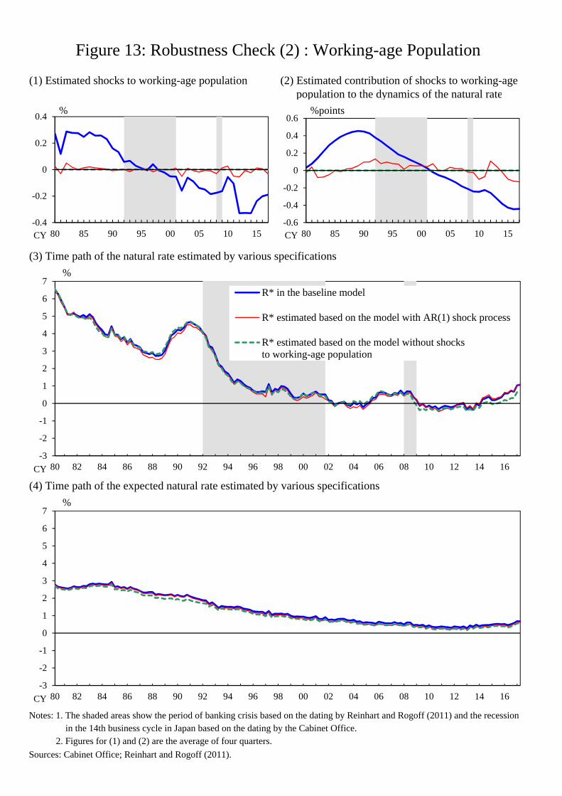
(1) Estimated shocks to working-age population (2) Estimated contribution of shocks to working-age(2) population to the dynamics of the natural rate

(3) Time path of the natural rate estimated by various specifications

(4) Time path of the expected natural rate estimated by various specifications

Notes: 1. The shaded areas show the period of banking crisis based on the dating by Reinhart and Rogoff (2011) and the recessionNotes: 1. in the 14th business cycle in Japan based on the dating by the Cabinet Office.Notes: 2. Figures for (1) and (2) are the average of four quarters.

Sources: Cabinet Office; Reinhart and Rogoff (2011).

Figure 13: Robustness Check (2) : Working-age Population

-0.4

-0.2

0

0.2

0.4

80 85 90 95 00 05 10 15

%

CY-0.6

-0.4

-0.2

0

0.2

0.4

0.6

80 85 90 95 00 05 10 15

%points

CY

-3

-2

-1

0

1

2

3

4

5

6

7

80 82 84 86 88 90 92 94 96 98 00 02 04 06 08 10 12 14 16

R* in the baseline model

R* estimated based on the model with AR(1) shock process

R* estimated based on the model without shocksto working-age population

%

CY

-3

-2

-1

0

1

2

3

4

5

6

7

80 82 84 86 88 90 92 94 96 98 00 02 04 06 08 10 12 14 16

%

CY