
Natural Hedging Using Multi-population Mortality...
67
Natural Hedging Using Multi-population Mortality Forecasting Models by Shuang Chen B.Sc., Nankai University, 2011 Thesis Submitted in Partial Fulfillment of the Requirements for the Degree of Master of Science in the Department of Statistics and Actuarial Science Faculty of Science © Shuang Chen 2014 SIMON FRASER UNIVERSITY Fall 2014 All rights reserved. However, in accordance with the Copyright Act of Canada, this work may be reproduced without authorization under the conditions for “Fair Dealing.” Therefore, limited reproduction of this work for the purposes of private study, research, criticism, review and news reporting is likely to be in accordance with the law, particularly if cited appropriately.
Transcript of Natural Hedging Using Multi-population Mortality...
Natural Hedging Using
Multi-population Mortality Forecasting Models
by
Shuang Chen
B.Sc., Nankai University, 2011
Thesis Submitted in Partial Fulfillment of the Requirements for the Degree of
Master of Science
in the
Department of Statistics and Actuarial Science
Faculty of Science
© Shuang Chen 2014 SIMON FRASER UNIVERSITY
Fall 2014
All rights reserved.
However, in accordance with the Copyright Act of Canada, this work may be
reproduced without authorization under the conditions for “Fair Dealing.”
Therefore, limited reproduction of this work for the purposes of private study,
research, criticism, review and news reporting is likely to be in accordance
with the law, particularly if cited appropriately.

APPROVAL
Name: Shuang Chen
Degree: Master of Science
Title: Natural Hedging Using Multi-population Mortality Fore-
casting Models
Examining Committee: Chair: Dr. Gary Parker
Associate Professor
Dr. Cary Chi-Liang Tsai
Senior Supervisor
Associate Professor
Simon Fraser University
Dr. Yi Lu
Supervisor
Associate Professor
Simon Fraser University
Dr. David Campbell
Internal Examiner
Associate Professor
Simon Fraser University
Date Approved: December 11th, 2014
ii

Partial Copyright Licence
iii
Abstract
No mortality projection model can capture future mortality changes accurately so
that the actual mortality rates are different from the projected ones. The movement
of mortality rates has oppositive impacts on the values of life insurance and annuity
products, which creates a chance of nature hedge for both life insurer and annuity
provider. A life insurer and an annuity provider can swap their life insurance and
annuity business for each other to form their own portfolios for natural hedge. This
project is mainly focused on determining the weights of a portfolio of life insurance
and annuity products by minimizing the variance of the loss function of the portfolio
to reduce mortality and longevity risks for each of the life insurer and the annuity
provider. Four Lee-Carter-based models are applied to model the co-movement
of two populations of life insurance and annuity insureds, and then determine the
weights for comparisons. The block bootstrap method, a model-/parameter-free
approach, is also adopted with numerical illustrations to compare the hedging per-
formances among the four models.
iv

I dedicate this thesis to my parents,
- who always support and cheer me up.
v

Acknowledgments
I would like to express my deepest appreciation to all those who supported and
guided me to complete this project. A special gratitude is given to my supervisor,
Dr. Cary Tsai, who provided me with patient guidance and valuable suggestions
that inspired me and helped me realize self-improvements throughout my two years
of studies in SFU. I will always be grateful to have the opportunity to learn new
ideas and conduct research under his supervision. Without his devoting time to
this project, I wouldn’t have completed the project. I hereby thank you for all your
time spent on guiding me.
Furthermore, I would also like to acknowledge with my great appreciation the
members of my project committee, Dr. Gary Parker, Dr. Yi Lu and Dr. David
Campbell. Thank you for reading my project with your valuable time and giving me
insightful comments and suggestions.
A special thank goes to the whole statistics and actuarial science department,
where I mastered more advanced knowledge that will benefit me forever. Thank
you to all the professors who have ever given me lectures and answered my ques-
tions. You helped me to fulfill a high level academic achievement.
Last but not least, I would like to take this opportunity to thank my family and my
friends who supported me and encouraged me whenever I felt confused and lost.
Especially, I would like to express my appreciation to my fellow graduate students,
Annie, Biljana, Elena, Fei, Huijing, Sabrina, Vicky and Yi, who brought me fresh
ideas and memorable moments during my study.
vi
Contents
Approval ii
Partial Copyright License iii
Abstract iv
Dedication v
Acknowledgments vi
Contents vii
List of Tables ix
List of Figures x
1 Introduction 1
1.1 Motivations . . . . . . . . . . . . . . . . . . . . . . . . . . . . . . . . 1
1.2 Outline . . . . . . . . . . . . . . . . . . . . . . . . . . . . . . . . . . . 2
2 Literature Review 4
2.1 Mortality forecasting models . . . . . . . . . . . . . . . . . . . . . . . 4
2.2 Hedging of mortality and longevity risks . . . . . . . . . . . . . . . . 6
3 Introduction of Multi-population Models 9
3.1 Concepts and notations . . . . . . . . . . . . . . . . . . . . . . . . . 9
3.2 Multi-population models and constrains . . . . . . . . . . . . . . . . 11
3.2.1 Independent Lee-Carter model . . . . . . . . . . . . . . . . . 11
3.2.2 Joint-k Lee-Carter model . . . . . . . . . . . . . . . . . . . . 16
3.2.3 Co-integrated model . . . . . . . . . . . . . . . . . . . . . . . 20
vii
3.2.4 Augmented common factor model . . . . . . . . . . . . . . . 23
4 Application in Mortality Swap 28
4.1 Natural hedging and mortality swap . . . . . . . . . . . . . . . . . . 28
4.2 Numerical illustrations . . . . . . . . . . . . . . . . . . . . . . . . . . 33
4.2.1 Assumptions and portfolios . . . . . . . . . . . . . . . . . . . 33
4.2.2 Robustness testing . . . . . . . . . . . . . . . . . . . . . . . . 36
5 Block Bootstrap Method 45
6 Conclusion 56
Bibliography 57
viii

List of Tables
4.1 the median of 50 optimal weights . . . . . . . . . . . . . . . . . . . . 37
4.2 comparisons of sample variances (×1023) and HE’s . . . . . . . . . 38
5.1 p-values for testing stationarity of {dx,t,i} . . . . . . . . . . . . . . . . 48
5.2 comparisons of sample variances (×1023) and HE’s (block bootstrap) 55
ix

List of Figures
3.1 cohort mortality sequence and period mortality sequence . . . . . . 10
3.2 kt,i against t . . . . . . . . . . . . . . . . . . . . . . . . . . . . . . . . 13
3.3 95% predictive intervals on qx,2009+1,i for the Independent model . . . 15
3.4 95% predictive intervals on qx,2009+1,i for the joint-k model . . . . . . 19
3.5 95% predictive intervals on qx,2009+1,2 for the co-integrated and inde-
pendent models . . . . . . . . . . . . . . . . . . . . . . . . . . . . . 22
3.6 95% predictive intervals on qx,2009+1,i for the augmented common fac-
tor model . . . . . . . . . . . . . . . . . . . . . . . . . . . . . . . . . 26
3.7 mortality curve comparisons among models and actual rates . . . . 27
4.1 Mortality swap: minimizing V ar(LL) + V ar(LA) . . . . . . . . . . . . 30
4.2 Mortality swap: minimizing V ar(LL) . . . . . . . . . . . . . . . . . . 30
4.3 Mortality swap: minimizing V ar(LA) . . . . . . . . . . . . . . . . . . 30
4.4 age span [25, 100] and year span [1981, 2010] . . . . . . . . . . . . . 35
4.5 optimal weights for the independent and joint-k models . . . . . . . . 39
4.6 optimal weights for the co-integrated and augmented common factor
models . . . . . . . . . . . . . . . . . . . . . . . . . . . . . . . . . . 40
4.7 variances after swap . . . . . . . . . . . . . . . . . . . . . . . . . . . 41
4.8 simulated loss distributions using (wL+Al , wL+A
a ) . . . . . . . . . . . . 42
4.9 simulated loss distributions using (wLl , w
La ) . . . . . . . . . . . . . . . 43
4.10 simulated loss distributions using (wAl , w
Aa ) . . . . . . . . . . . . . . . 44
5.1 {dx,t,i} for x = 35, 45, 55, 65 . . . . . . . . . . . . . . . . . . . . . . . . 47
5.2 a circle diagram of dt,i’s . . . . . . . . . . . . . . . . . . . . . . . . . 49
5.3 simulated loss distributions using (wL+Al , wL+A
a ) . . . . . . . . . . . . 52
5.4 simulated loss distributions using (wLl , w
La ) . . . . . . . . . . . . . . . 53
5.5 simulated loss distributions using (wAl , w
Aa ) . . . . . . . . . . . . . . . 54
x

Chapter 1
Introduction
1.1 Motivations
Natural hedging is a strategy of hedging two risks responding oppositely to a
change in a common factor. Since life insurers and annuity providers face mor-
tality risk (the actual death probabilities are higher than expected) and longevity
risk (the actual survival probabilities are larger than expected), respectively, both
of them can adopt natural hedging by swapping a portion of their business between
each other to reduce mortality and longevity risks.
In this project, we would like to find the optimal swapped weights of life and
annuity business for a life insurer and an annuity provider, respectively, which min-
imize the variance of a loss function of the life insurer or the annuity provider, or
the sum of the variances of the two loss functions. To reach the goal, we need
some mortality models to forecast mortality rates for life insurance policyholders
and annuitants.
Since life insurance and annuities tend to be issued to different populations,
using the same mortality table to determine the premiums is inappropriate. Fur-
thermore, even though we use two different mortality tables for life insurance pol-
icyholders and annuitants, we cannot ignore the dependence between these two
populations. Generally speaking, two populations within a territory or country are
exposed to the same medical and environmental conditions. Therefore, the mortal-
ity rates for two populations might not be independent. In this project, two different
1

CHAPTER 1. INTRODUCTION 2
mortality tables and four multi-population mortality models are applied to forecast-
ing deterministic and stochastic mortality rates.
The deterministic mortality rates are used to determine the premiums of life and
annuity products, and the stochastic mortality ones are used to simulate the losses
of the life insurer and annuity provider. Then we calculate the sample variances
and sample covariance of the losses of the life insurer and annuity provider for ob-
taining the formulas of the optimal weights. A variance reduction ratio, called hedge
effectiveness, is proposed to compare the performances of hedging mortality and
longevity risks.
This project also carries out the robustness testing to study the sensitivity of
the weights and variances obtained from the simulated mortality rates. Finally, be-
cause all the results are derived based on the parametric mortality models, we are
not sure whether the assumed mortality model is the true one. To avoid the pa-
rameter and model risks, the model-free block bootstrap method is used to project
mortality rates. Then we redo the numerical results which are compared with those
produced by the parametric mortality models.
1.2 Outline
This project consists 5 chapters. Chapter 2 is a review of the previous research on
both mortality projection models and hedging of mortality and longevity risks.
In Chapter 3, some actuarial notations used in this project are provided, fol-
lowed by the introduction of four mortality projection models, the independent Lee-
Carter model, joint-k Lee-Carter model, co-integrated Lee-Carter model and aug-
mented common factor model, among which the last three can model the depen-
dent structure between the mortality rates for two populations. These models can
be used to forecast deterministic and stochastic mortality rates for both life insur-
ance policyholders and annuitants.

CHAPTER 1. INTRODUCTION 3
Chapter 4 focuses on natural hedging with mortality swap. In this chapter, three
pairs of optimal weights for swapping life insurance and annuity business are stud-
ied. Numerical illustrations using the U.S. mortality tables are exhibited. Also, the
robustness testing is conducted to test the sensitivity of the numerical results.
In Chapter 5, the model free block bootstrap method is introduced in details,
which is then applied to testing the results produced by the multi-population models
in Chapter 4.
Chapter 2
Literature Review
The two main parts of this project are mortality projection and natural hedge. The
first section will go through the articles about the mortality forecasting models and
the second section will review those about hedging of mortality and longevity risks.
2.1 Mortality forecasting models
Mortality projection is one of the keys for pricing insurance and annuity products.
The most widely used mortality projection model so far is the Lee-Carter model
(Lee and Carter (1992)). Between 1900 and 1988, the life expectancy in the United
States increased from 47 to 75. Based on the assumption that the life expectancy
would continue to increase, Lee and Carter (1992) applied the time series model to
forecasting long term mortality rates. This model considers two age-varying factors
and one time-varying factor to capture the downward trend in mortality rates. By
empirical mortality data, it is assumed that the time-varying factor is fitted by an
ARIMA (autoregressive integrated moving average) model.
One of the most significant features of the Lee-Carter model is that it is easy to
interpret and its parameters are estimable. Compared to other mortality projection
models, the Lee-Carter model bases its forecast on long term historical data, and
no explicit assumptions or a life span limit is attached to the model. Moreover, the
Lee-Carter model provides confidence regions, which was further proved that the
model is efficient in forecasting mortality rates.
4

CHAPTER 2. LITERATURE REVIEW 5
Afterwards, Lee and Carter (1992) pointed out that in order to forecast the mor-
tality rates for two populations within a territory or country, the same time-varying
index, called joint-k index, should be used so that the same trend of mortality
growth in response to time for the two populations can be reflected. This assump-
tion makes sense because usually two populations in a country have the same
medical service and environmental condition, etc. Thus, when these aspects im-
prove, the life expectancy of each population will increase simultaneously to the
same level.
Lee and Li (2005) extended the original Lee-Carter model by adding an extra
term to the model. They thought that the world is becoming more closely con-
nected by modern communication technology. Thus, in a long term, the forecasted
mortality rates for different populations will converge. They called it the augmented
common factor model, which was developed in two steps. Firstly, Lee and Li (2005)
used a common factor to capture the overall mortality growth; then the mortality
rates of that population are specified by an augmented term which reflects the fea-
ture of that population. This method was applied to forecasting the mortality rates
of Canadian populations. In different provinces, the common factor was used to
realize the long term convergence, and the augmented term was used to separate
the mortality rates for each province.
With the same concern about the long-term convergence problem, Li and Hardy
(2011) suggested the so-called co-integrated Lee-Carter model. By investigating
the time-varying indices of two populations, they noticed that there exists a co-
integrated relationship between the two time indices. In the co-integrated model,
two time-varying indices are modeled by a linear function.
The last three mentioned models based on the Lee-Carter model all take into
consideration the dependent structures among multiple populations; we call them
the multi-population mortality projection models. In this project, because the natu-
ral hedging strategy is adopted by swapping portions of life and annuity business
based on two populations of life insurance policyholders and annuitants, the multi-
population mortality projection models are needed.

CHAPTER 2. LITERATURE REVIEW 6
2.2 Hedging of mortality and longevity risks
Hedging of mortality and longevity risks is one of the most popular research areas
recently in Actuarial Science. Researchers have conducted large amount of study
on how to reduce mortality and longevity risks. Some of the financial instruments
have been applied to hedging these two risks, such as mortality-linked securities,
q-forward, etc. The practice of using mortality-linked securities was first suggested
by Blake and Burrows (2001) by pouring longevity risk into the capital market.
They introduced a survivor bond for which the future coupons are based on the
percentage of the alive retirees at the future coupon payments dates.
In 2003, Swiss Re issued the first mortality-linked security which is to protect
insurers from the loss of catastrophes. The bonds were issued via SPV (special
purpose vehicle). The payments depend on a mortality index. This bond has been
successfully operated for years.
BNP-Paribas and the European Investment Bank in 2004 issued a 25-year
longevity bond to hedge longevity risks. This is the first longevity bond that came
into real business. The coupons were linked to the survivor index based on the
actual mortality rates of England and Welsh males aged 65 in 2002.
In 2006, a pension buyout market attracted a lot of attention in UK. In this market
both the assets and liabilities of a pension plan were transferred to a life insurer.
To realize the transfer, the pension plan has to pay the life insurer the amount of
deficit if the assets are less than the liabilities. On the contrary, the insurer will pay
the surplus to the pension plan if assets exceeds liabilities. Thus, the pension plan
can be secured. This is an efficient method of transferring longevity risk; however,
the pension plan will possibly experience loss since the life insurer tends to re-
evaluate the pension plan by measuring the assets and liability in a way of more
risk aversion.
In 2007, J.P. Morgan introduced q-forwards, another financial derivatives, to
transfer mortality rates to the capital market. The q-forwards are described as a
zero coupon swap between a pre-fixed mortality rate at inception date and the
realized mortality rate at maturity date of the q-forward contract.

CHAPTER 2. LITERATURE REVIEW 7
Not only the pricing and structure of the mortality-linked securities have been
systematically studied but also how to evaluate the hedging methodology. Li and
Ng (2011) pointed out that because of lack of longevity trading index from which to
evolve the market price of the mortality-linked securities, it still remains a question
of how to evaluate the hedging technics. Thus, they proposed a pricing framework
for evaluating the mortality-linked securities based on canonical valuation. To con-
struct the framework, they suggested a nonparametric model, which helps to avoid
the risks from model itself and its parameters.
Gaillardetz et al. (2012) proposed a method of evaluating the hedging error
under a stochastic mortality projection. It is very likely that when catastrophes
occur insurers would experience huge amount of losses. Thus, evaluating the
distribution of hedging error is very important. They applied the regime-switching
model (Milidonis et al. (2011)) to extracting the hedging error and conducted the
error distribution that made the evaluation feasible.
In recent years, another kind of hedging method called natural hedge has be-
come appealing for researchers. Because instead of transferring the risk into fi-
nancial market, natural hedge can reduce mortality and longevity risks simply by
swapping proportions of life and annuity business between a life insurer and an an-
nuity provider. Cox and Lin (2007) are the first to thoroughly introduce this concept
by noticing the empirical evidence that companies adopting natural hedge within
their business usually offer lower premiums than the other companies.
After the proposal of natural hedge, tons of studies have been done in this field.
Wang et al. (2010) suggested that by mortality duration and convexity matching,
the optimal weights for conducting an immunization portfolio can be obtained. Lin
and Tsai (2013) gave more elaborate formulas for mortality duration and convexity,
which can be applied to a two-product or three-product portfolio.
However, some researchers also threw doubt on natural hedging that all the
studies are based on some models, but in reality the future mortality rates might be
totally model free, which may cause the method inefficient. Zhu and Bauer (2014)
used a non-parametric model to test the natural hedge method and came to the
conclusion that higher order variations in mortality rates would affect the efficiency
of natural hedging. Another problem of natural hedging pointed out by Cox and Lin

CHAPTER 2. LITERATURE REVIEW 8
(2007) is that for estimating the future mortality rates, most of the studies use the
same life table for both annuity and life insurance, which is not practical.
This project uses multi-population mortality projection models to forecast future
mortality rates for life insurance policyholders and annuitants separately based
on two life tables. The method of Langrage multipliers is used to help obtain the
optimal weights. Moreover, robust testing, together with model testing based on
the model-free block bootstrap method, is carried out.

Chapter 3
Introduction of Multi-populationModels
In this chapter, we first introduce four mortality models for multi-populations, which
are based on the well known Lee-Carter model. Then we fit the models with mor-
tality data from the Human Mortality Database to get the estimated parameters
which can be applied to forecasting future mortality rates. The deterministic mor-
tality rates can be used to determine the prices of life insurance and annuity prod-
ucts, and the stochastic ones can be used to simulate the realized/actual prices in
Chapter 4.
3.1 Concepts and notations
Let qx,t,i denote the probability that an individual aged x in year t for population
i will die within one year. We add an extra subscript i for studying the multi-
population mortality projection models. When forecasting the future mortality rates,
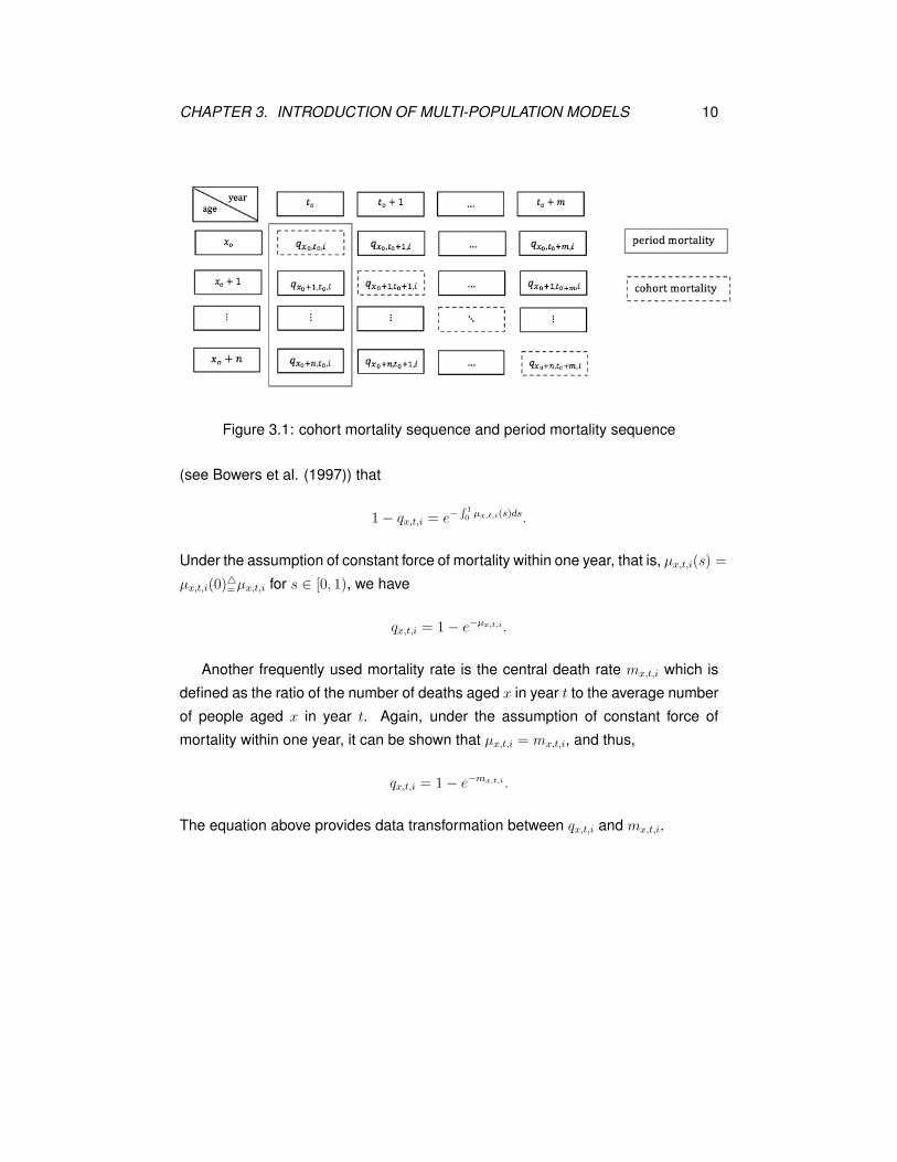
there are mainly two types of mortality sequences. One is the cohort mortality se-
quence {qx0+j,t0+j,i : j = 0, 1, 2, ...}, and the other is the period mortality sequence
{qx0+j,t0,i : j = 0, 1, 2, ...}. In this project, the cohort mortality sequence is used
for pricing. Figure 3.1 shows the difference between the cohort mortality sequence
and the period one.
Next, denote μx,t,i(s) the function of force of mortality, which is an instantaneous
death rate between age x and x+s in year t for population i aged x. It can be shown
9
CHAPTER 3. INTRODUCTION OF MULTI-POPULATION MODELS 10
Figure 3.1: cohort mortality sequence and period mortality sequence
(see Bowers et al. (1997)) that
1− qx,t,i = e−∫ 10 μx,t,i(s)ds.
Under the assumption of constant force of mortality within one year, that is, μx,t,i(s) =
μx,t,i(0)�=μx,t,i for s ∈ [0, 1), we have
qx,t,i = 1− e−μx,t,i .
Another frequently used mortality rate is the central death rate mx,t,i which is
defined as the ratio of the number of deaths aged x in year t to the average number
of people aged x in year t. Again, under the assumption of constant force of
mortality within one year, it can be shown that μx,t,i = mx,t,i, and thus,
qx,t,i = 1− e−mx,t,i .
The equation above provides data transformation between qx,t,i and mx,t,i.

CHAPTER 3. INTRODUCTION OF MULTI-POPULATION MODELS 11
3.2 Multi-population models and constrains
3.2.1 Independent Lee-Carter model
Lee and Carter (1992) proposed a model that the natural logarithm of central death
rates can be expressed by two age specific factors and one time specific factor as
follows:
ln(mx,t,i) = ax,i + bx,i × kt,i + εx,t,i,
subject to two constraints,
• ∑x bx,i = 1,
and
• ∑t kt,i = 0,
where
• ax,i is the average age-specific mortality factor at age x for population i,
• kt,i is the general mortality level in year t for population i,
• bx,i is the age-specific reaction to kt,i at age x for population i, and
• εx,t,i is the error term which is assumed independent and identically normally
distributed with mean 0 and variance σ2εx,i
for all t′s.
To fit the model with a given matrix of ln(mx,t,i)′s for population i and estimate
all parameters, we may use the singular value decomposition (SVD) method. How-
ever, there is a close approximation to SVD.
First, ax,i can be derived by the average of the sum of ln(mx,t,i) over a given year
span [t0, t0+n−1] by the second constraint, and kt,i equals the sum of [ln(mx,t,i)−ax,i] over a given age span [x0, x0 +m− 1] by the first constraint. That is,
t0+n−1∑
t=t0
ln(mx,t,i) = n× ax,i + bx,i ×t0+n−1∑
t=t0
kt,i = n× ax,i,
CHAPTER 3. INTRODUCTION OF MULTI-POPULATION MODELS 12
implying
ax,i =
∑t0+n−1t=t0
ln(mx,t,i)
n, x = x0, x0 + 1, ...., x0 +m− 1.
Similarly,
x0+m−1∑
x=x0
[ln(mx,t,i)− ax,i] = kt,i ×x0+m−1∑
x=x0
bx,i,
yielding
kt,i =
x0+m−1∑
x=x0
[ln(mx,t,i)− ax,i], t = t0, t0 + 1, ..., t0 + n− 1.
Finally, bx,i can be obtained by regressing [ln(mx,t,i) − ax,i] on kt,i without the
constant term involved for each age x. For projecting the future time-varying index
kt,i, a key to project the mortality rates, an ARIMA(0,1,0) time series (a random
walk with drift θi) is used, which is given by
kt,i = kt−1,i + θi + εt,i,
where the error term εt,i follows an independent and identical normal distribution
with mean 0 and variance σ2ε,i for all t′s. The parameter θi can be estimated by
θi =1
n− 1
t0+n−1∑
t=t0+1
(kt,i − kt−1,i) =kt0+n−1,i − kt0,i
n− 1.
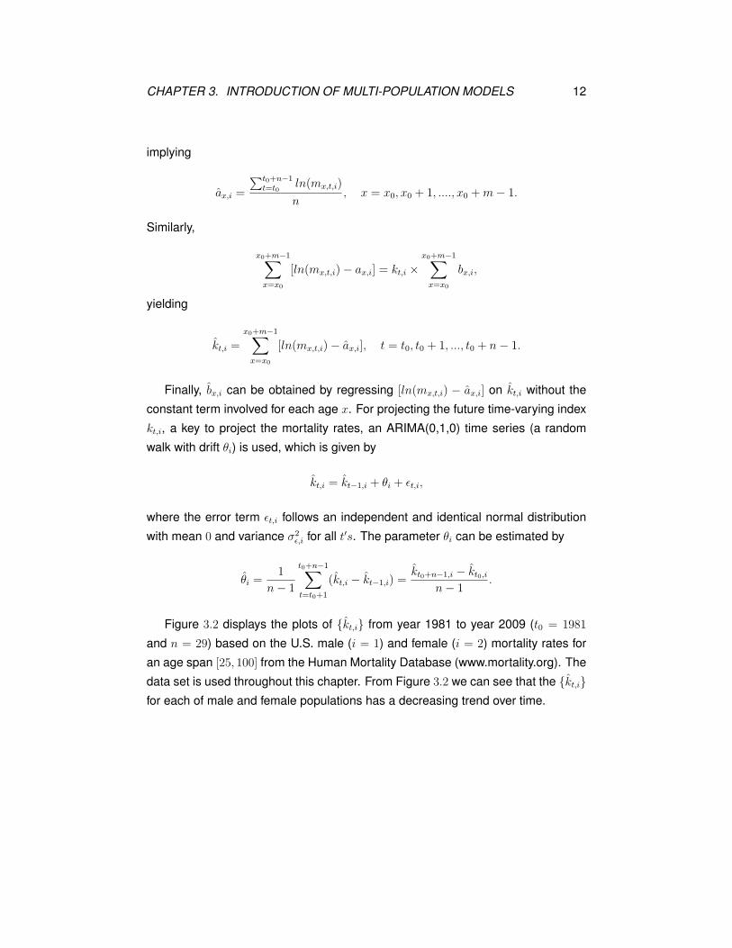
Figure 3.2 displays the plots of {kt,i} from year 1981 to year 2009 (t0 = 1981
and n = 29) based on the U.S. male (i = 1) and female (i = 2) mortality rates for
an age span [25, 100] from the Human Mortality Database (www.mortality.org). The
data set is used throughout this chapter. From Figure 3.2 we can see that the {kt,i}for each of male and female populations has a decreasing trend over time.

CHAPTER 3. INTRODUCTION OF MULTI-POPULATION MODELS 13
Figure 3.2: kt,i against t
The logarithm of the stochastic central death rate for age x in year t0+n− 1+ τ
denoted by mx,t0+n−1+τ,i is
ln(mx,t0+n−1+τ,i) =ax,i + bx,i × (kt0+n−1,i + τ × θi +√τ × εt,i) + εx,t,i
=ln(mx,t0+n−1+τ,i) +√τ × bx,i × εt,i + εx,t,i,
where mx,t0+n−1+τ,i is the deterministic central death rate. Note that ln(mx,t0+n−1+τ,i)
is normally distributed with mean
ln(mx,t0+n−1+τ,i) = ax,i + bx,i × (kt0+n−1,i + τ × θi), τ = 1, 2, ....
and variance σ2(ln(mx,t0+n−1+τ,i)) = τ × b2x,i × σ2ε,i + σ2
εx,i, where {εx,t,i} and {εt,i}
are assumed independent.
Then
mx,t0+n−1+τ,i = exp[ax,i + bx,i × (kt0+n−1,i + τ × θi)],
or
qx,t0+n−1+τ,i = 1− exp[−exp(ax,i + bx,i × (kt0+n−1,i + τ × θi))].

CHAPTER 3. INTRODUCTION OF MULTI-POPULATION MODELS 14
The estimate of the variance of εx,t,i is given by
σ2εx,i
=1
n− 2
t0+n−1∑
t=t0
ε2x,t,i =
∑t0+n−1t=t0
[ln(mx,t,i)− ax,i − bx,i × kt,i]2
n− 2,
where x = x0, x0 + 1, ..., x0 +m− 1. The estimate of the variance of εt,i is given as
σ2ε,i =
1
n− 2
t0+n−1∑
t=t0+1
ε2t,i =
∑t0+n−1t=t0+1 (kt,i − kt−1,i − θi)
2
n− 2.
Therefore, the estimate of the variance of ln(mx,t0+n−1+τ,i) is obtained by
σ2(ln(mx,t0+n−1+τ,i))�= σ
2x,t0+n−1+τ,i = τ × b2x,i × σ2
ε,i + σ2εx,i
,
and a 100(1− γ)% predictive interval on qx,t0+n−1+τ,i can be constructed as
1− exp[−exp(ln(mx,t0+n−1+τ,i)± z γ2× σx,t0+n−1+τ,i)].
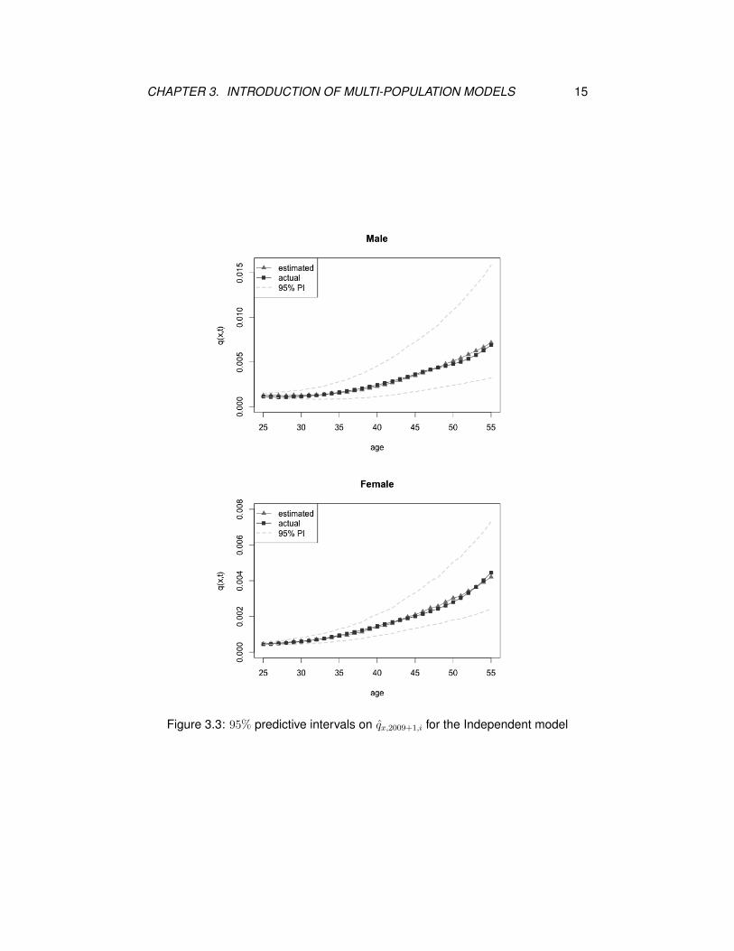
Figure 3.3 shows the projected period mortality rates in year 2010 based on the
central death rates from year 1981 to 2009. It is obvious that the estimated mor-
tality rates are quite close to the actual ones, and a narrower predictive interval on
the female mortality rates than that on the male ones is produced.
CHAPTER 3. INTRODUCTION OF MULTI-POPULATION MODELS 15
Figure 3.3: 95% predictive intervals on qx,2009+1,i for the Independent model

CHAPTER 3. INTRODUCTION OF MULTI-POPULATION MODELS 16
3.2.2 Joint-k Lee-Carter model
Apparently, two independent models ignore the co-movements between the mor-
tality rates for two populations. The males and females in a country live in the
same environment, and their mortality rates are affected by some common fac-
tors. To relate one population’s mortality rates to the other’s ones, Carter and
Lee (1992) introduced the joint-k model where the time-varying index kt,i, which
shows the general mortality level over time, is the same for both populations, that
is, kt,1 = kt,2 = Kt. The model can be expressed as
ln(mx,t,i) = ax,i + bx,i ×Kt + εx,t,i, i = 1, 2,
subject to two new constraints:
• ∑2i=1
∑x bx,i = 1
and
• ∑t Kt = 0.
Similarly, ax,i can be derived by the average of the sum of ln(mx,t,i) over a year
span [t0, t0+n−1], and Kt is equal to the sum of [ln(mx,t,i)− ax,i] over an age span
[x0, x0 +m− 1] and the population index. That is,
t0+n−1∑
t=t0
ln(mx,t,i) = n× ax,i + bx,i ×t0+n−1∑
t=t0
Kt,
implying
ax,i =
∑t0+n−1t=t0
ln(mx,t,i)
n, x = x0, x0 + 1, ..., x0 + n− 1;
and2∑
i=1
x0+m−1∑
x=x0
ln(mx,t,i) =2∑
i=1
x0+m−1∑
x=x0
ax,i +2∑
i=1
x0+m−1∑
x=x0
bx,i ×Kt,
giving
Kt =2∑
i=1
x0+m−1∑
x=x0
[ln(mx,t,i)− ax,i], t = t0, t0 + 1, ..., t0 + n− 1.
As for bx,i, it is obtained by regressing [ln(mx,t,i) − ax,i] on Kt without the constant
term involved for each age x. The common time-varying index Kt is also assumed

CHAPTER 3. INTRODUCTION OF MULTI-POPULATION MODELS 17
to follow a random walk with drift θ. That is
Kt = Kt−1 + θ + εt,
where the error term εt follows an independent and identical normal distribution
with mean 0 and variance σ2ε , and εt is independent of εx,t,i. The parameters θ is
estimated by
θ =Kt0+n−1 − Kt0
n− 1.
The logarithm of the forecasted central death rate for age x in year t0 + n− 1+ τ is
ln(mx,t0+n−1+τ,i) = ax,i + bx,i × (Kt0+n−1 + τ × θ +√τ × εt,i) + εx,t,i
= ln(mx,t0+n−1+τ,i) +√τ × bx,i × εt,i + εx,t,i,
where
ln(mx,t0+n−1+τ,i) = ax,i + bx,i × (Kt0+n−1 + τ × θ), τ = 1, 2, ....
The estimate of the variance of εx,t,i is
σ2εx,i
=
∑t0+n−1t=t0
[ln(mx,t,i)− ax,i − bx,i × Kt]2
n− 2,
and the estimate of the variance of εt is
σ2ε =
∑t0+n−1t=t0+1 (Kt − Kt−1 − θ)2
n− 2.
Thus, the variance of ln(mx,t0+n−1+τ,i) is
σ2x,t0+n−1+τ,i = τ × b2x,i × σ2
ε + σ2εx,i
,
which can be used to construct a 100(1− γ)% predictive interval on qx,t0+n−1+τ,i as
1− exp[−exp(ln(mx,t0+n−1+τ,i)± z γ2× σx,t0+n−1+τ,i)].
Using the same data set as that for Figure 3.3, we display corresponding forecasted
mortality rates and associated predictive intervals based on the joint-k model in

CHAPTER 3. INTRODUCTION OF MULTI-POPULATION MODELS 18
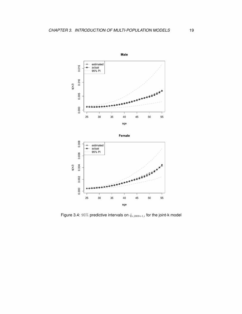
Figure 3.4. The projected mortality rates and the predictive interval are almost the
same with those for the independent model, where the estimated mortality rates
are close to actual ones, and the 95% predictive interval on the male mortality rates
is wider than that on the female ones.
CHAPTER 3. INTRODUCTION OF MULTI-POPULATION MODELS 19
Figure 3.4: 95% predictive intervals on qx,2009+1,i for the joint-k model
CHAPTER 3. INTRODUCTION OF MULTI-POPULATION MODELS 20
3.2.3 Co-integrated model
In the joint-k model, two populations share the same time-varying index Kt. In the
co-integrated model, the time-varying index for population 2 is a linear function of
the time-varying index for population 1. Specifically, assume the mortality rates for
populations 1 and 2 are modeled by
ln(mx,t,1) = ax,1 + bx,1 × kt,1 + εx,t,1
and
ln(mx,t,2) = ax,2 + bx,2 × kt,2 + εx,t,2.
By fitting the model with given data, kt,1 and kt,2 can be estimated separately in
the same way as those for two independent Lee-Carter models. Under the co-
integrated model, we assume there is a linear relationship plus an error term et
between kt,1 and kt,2, that is,
kt,2 = α + β × kt,1 + et. (3.1)
Since kt,1 and kt,2 are known, the estimates of parameters α and β can be obtained
by simple linear regression method. To build the link between kt,1 and kt,2, the co-
integrated model suggests re-estimating kt,2 to get ˆkt,2 with kt,1 unchanged using
(3.1) by plugging in the values of α and β. That is,
ˆkt,2 = α + β × kt,1.
In the co-integrated model, the estimates of the two variances for population 1,
σ2εx,1
and σ2ε,1, are the same as those for the original Lee-Carter model. However,
for the second population, the drift of the time-varying index is estimated by
θ2 =ˆkt0+n−1,2 − ˆ
kt0,2n− 1
= β × kt0+n−1,1 − kt0,1n− 1
= β × θ1,
CHAPTER 3. INTRODUCTION OF MULTI-POPULATION MODELS 21
and the estimate of the variance of the error term for the time-varying index is
σ2ε,2 =
∑t0+n−1t=t0+1 (
ˆkt,2 − ˆ
kt−1,2 − θ2)2
n− 2
= β2 ×t0+n−1∑
t=t0+1
(kt,1 − kt−1,1 − θ1)2
n− 2
= β2 × σ2ε,1.
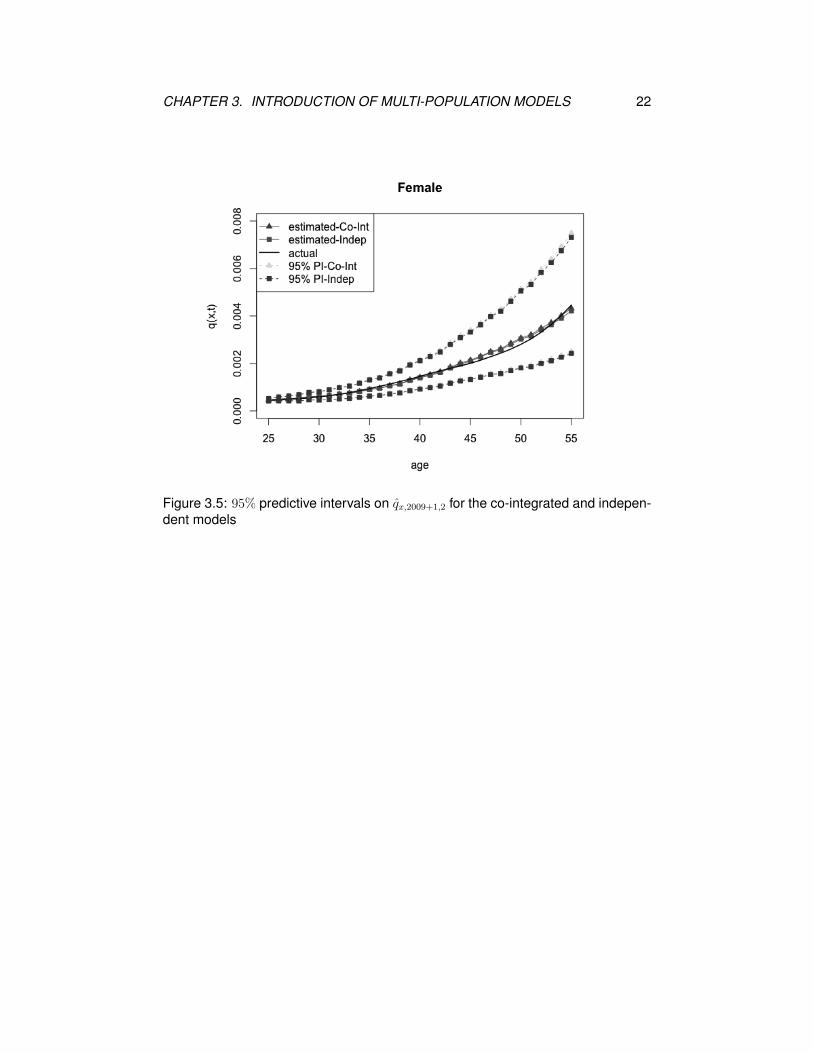
The expression of the predictive interval on qx,t0+n−1+τ,i is still the same as that
for independent Lee-Carter model. Figure 3.5 is the forecasted mortality rates
qx,2009+1,2 (female, τ = 1) and the associated 95% predictive intervals for the co-
integrated model as well as the corresponding one for the independent model for
comparison. We can see that both the forecasted mortality rates and predictive
intervals for both models are quite close to each other. Starting from age 40, the
forecasted mortality rates for the co-integrated model become slightly higher than
those for the independent model. The predictive intervals for both models almost
overlap.
CHAPTER 3. INTRODUCTION OF MULTI-POPULATION MODELS 22
Figure 3.5: 95% predictive intervals on qx,2009+1,2 for the co-integrated and indepen-dent models
CHAPTER 3. INTRODUCTION OF MULTI-POPULATION MODELS 23
3.2.4 Augmented common factor model
To avoid divergence in life expectancy in a long-run, Lee and Li (2005) suggested
adding a common factor to the original model. For the common term, it has the
following features:
• bx,1 = bx,2 = Bx for all x, and
• for the time-varying index, kt,1 = kt,2 = Kt for all t.
Two similar constrains apply, which are
• ∑2i=1
∑x wi × Bx = 1
and
• ∑t Kt = 0,
where w1 and w2 are the weights for populations 1 and 2, respectively, and w1+w2 =
1. Thus, the common factor model can be expressed as
ln(mx,t,i) = ax,i +Bx ×Kt + εx,t,i.
According to Li and Lee (2005), ax,i can still be derived by averaging ln(mx,t,i)
over a year span [t0, t0 + n− 1], that is,
t0+n−1∑
t=t0
ln(mx,t,i) =
t0+n−1∑
t=t0
ax,i +Bx ×t0+n−1∑
t=t0
Kt,
implying
ax,i =
∑t0+n−1t=t0
ln(mx,t,i)
n,
and Kt is obtained by
2∑
i=1
x0+m−1∑
x=x0
wi × [ln(mx,t,i)− ax,i] = Kt ×2∑
i=1
x0+m−1∑
x=x0
wi ×Bx,
yielding
Kt =2∑
i=1
x0+m−1∑
x=x0
wi × [ln(mx,t,i)− ax,i].
CHAPTER 3. INTRODUCTION OF MULTI-POPULATION MODELS 24
We set w1 = w2 = 0.5 for the U.S. male and female life tables. Since
2∑
i=1
wi × [ln(mx,t,i)− ax,i] = Bx × Kt ×2∑
i=1
wi = Bx × Kt,
we regress∑2
i=1 wi × [ln(mx,t,i) − ax,i] on Kt to get Bx for each age x. To fit the
data better, Li and Lee (2005) added a factor b′x,i × k′t,i for each population to the
common factor model to form the so-called augmented common factor model as
ln(mx,t,i) = ax,i +Bx ×Kt + b′x,i × k
′t,i + εx,t,i, i = 1, 2,
with an extra constrain∑
x b′x,i = 1. Notice that b′x,i and k
′t,i here are different from
bx,i and kt,i in the independent model. The constrain∑
x bx,i = 1 implies that
k′t,i =
x0+m−1∑
x=x0
[ln(mx,t,i)− ax,i − Bx × Kt].
Finally, b′x,i is derived by regressing [ln(mx,t,i) − ax,i − Bx × Kt] on k′t,i without the
constant term involved for each age x.
The logarithm of the forecasted central death rate for age x in year t0+n−1+ τ
is
ln(mx,t0+n−1+τ,i) =ax,i + Bx × (Kt0+n−1 + τ × θ +√τ × εt)
+ b′x,i × (k
′t0+n−1,i + τ × θi +
√τ × εt,i) + εx,t,i
=ln(mx,t0+n−1+τ,i) +√τ × (Bx × εt + b
′x,i × εt,i) + εx,t,i
which is normal with mean
ln(mx,t0+n−1+τ,i) = ax,i + Bx × (Kt0+n−1 + τ × θ) + b′x,i × (k
′t0+n−1,i + τ × θi),
and variance
σ2(ln(mx,t0+n−1+τ,i)) = τ × (Bx × σ2ε + b
′2x,i × σ2
ε,i) + σ2εx,i
CHAPTER 3. INTRODUCTION OF MULTI-POPULATION MODELS 25
where the three error terms, {εx,t,i}, {εt} and {εt,i}, are assumed independent,
θ =Kt0+n−1 − Kt0
n− 1
and
θ′i =
k′t0+n−1 − k
′t0
n− 1, i = 1, 2.
To construct the predictive intervals and simulate mortality rates, we need the esti-
mates of σ2εx,i
, σ2ε and σ2
ε,i, which are
σ2εx,i
=
∑t0+n−1t=t0
[ln(mx,t,i)− ax,i − Bx × Kt − b′x,i × k
′t,i]
2
n− 3, i = 1, 2,
σ2ε =
∑t0+n−1t=t0+1 (Kt − Kt−1 − θ)2
n− 2,
and
σ2ε,i =
∑t0+n−1t=t0+1 (k
′t,i − k
′t−1,i − θ
′i)
2
n− 2, i = 1, 2.
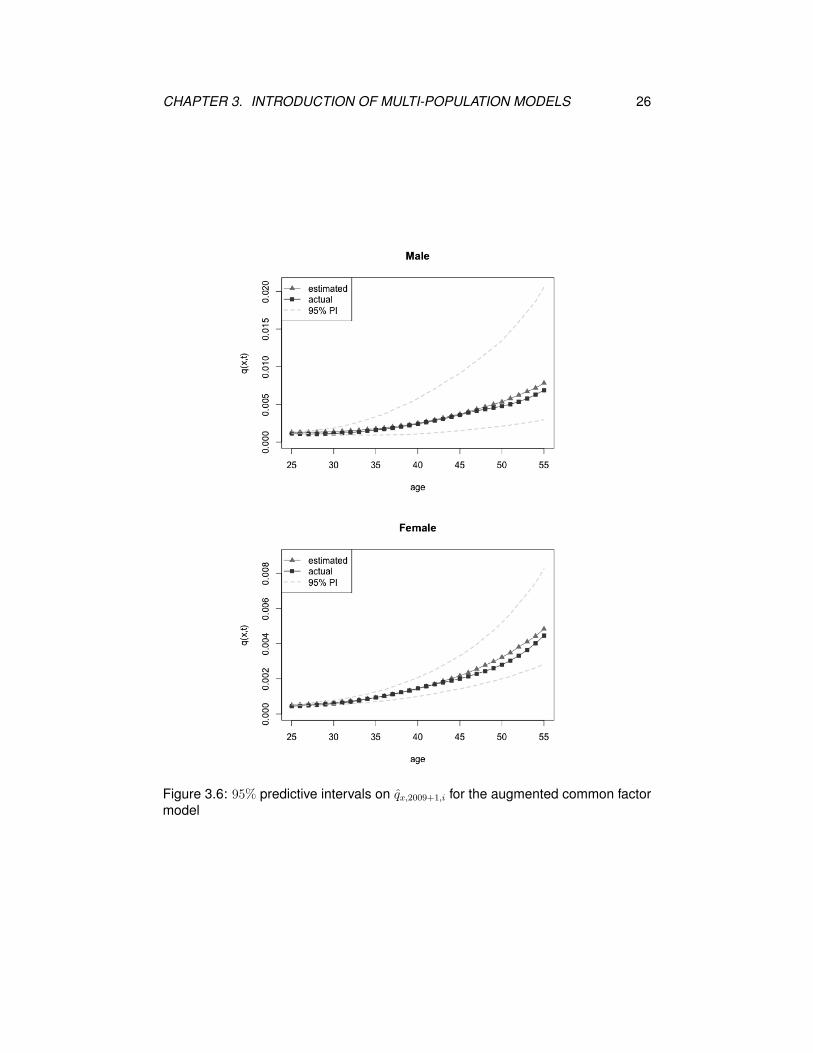
Figure 3.6 displays the forecasted qx,2009+1,i and associated predictive intervals
as well as the actual qx,2009+1,i for the augmented common factor model. When x
is small, the forecasted values are quite close to the true values. However, when
x goes up, the projected mortality rates tend to be higher than the actual ones.
Again, the predicted interval for the females is narrower than that for the males.
CHAPTER 3. INTRODUCTION OF MULTI-POPULATION MODELS 26
Figure 3.6: 95% predictive intervals on qx,2009+1,i for the augmented common factormodel

CHAPTER 3. INTRODUCTION OF MULTI-POPULATION MODELS 27
Figure 3.7 compares the predicted mortality rates among four models with the
actual mortality rates for year 2010 (τ = 1). It is obvious that all forecasted values
are close to actual ones for small x. We notice that the forecasted values from the
joint-k model are closer to the true values, while the mortality curve constructed
from the augmented common factor model is not as adjacent to the actual mortality
curve as the other models.
Figure 3.7: mortality curve comparisons among models and actual rates

Chapter 4
Application in Mortality Swap
4.1 Natural hedging and mortality swap
Mortality (longevity) risk is the risk that the number of deaths (survivors) is higher
than expected. When there is an unexpected change in mortality rates, either
life insurers or annuity providers will experience a loss. If the mortality rates in-
crease unexpectedly in a year, the number of deaths during the year is higher
than expected so that life insurance companies need to pay more death benefits.
However, in this case, annuity providers gain from the mortality increase. If the
mortality rates decline unexpectedly, the impacts on financial situation of life in-
surers and annuity providers reverse. Natural hedge is a strategy of hedging two
risks responding oppositely to a change in a common factor. Since life insurers
and annuity providers face mortality and longevity risks, respectively, both of them
can adopt natural hedge by swapping a portion of their business each other. When
a life insurer (an annuity provider) owns both life and annuity business at the same
time, the mortality and longevity risks of the portfolio can be offset to a lower level
no matter how the mortality rates change. Now, a question rises: what are the opti-
mal portions of business swapped between the life insurer and the annuity provider
such that the risk of the portfolio is minimized?
Let L denote the loss function at time zero, which is the present value of future
liabilities less the present value of future premium incomes. The values of both
future liabilities and premium incomes depend on the future mortality rates. Before
swapping the business, a life insurer (an annuity provider) has a portfolio of life
28
CHAPTER 4. APPLICATION IN MORTALITY SWAP 29
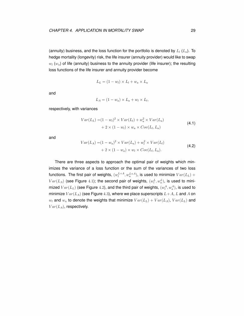
(annuity) business, and the loss function for the portfolio is denoted by Ll (La). To
hedge mortality (longevity) risk, the life insurer (annuity provider) would like to swap
wl (wa) of life (annuity) business to the annuity provider (life insurer); the resulting
loss functions of the life insurer and annuity provider become
LL = (1− wl)× Ll + wa × La
and
LA = (1− wa)× La + wl × Ll,
respectively, with variances
V ar(LL) =(1− wl)2 × V ar(Ll) + w2
a × V ar(La)
+ 2× (1− wl)× wa × Cov(Ll, La)(4.1)
andV ar(LA) =(1− wa)
2 × V ar(La) + w2l × V ar(Ll)
+ 2× (1− wa)× wl × Cov(Ll, La).(4.2)
There are three aspects to approach the optimal pair of weights which min-
imizes the variance of a loss function or the sum of the variances of two loss
functions. The first pair of weights, (wL+Al , wL+A
a ), is used to minimize V ar(LL) +
V ar(LA) (see Figure 4.1); the second pair of weights, (wLl , w
La ), is used to mini-
mized V ar(LL) (see Figure 4.2), and the third pair of weights, (wAl , w
Aa ), is used to
minimize V ar(LA) (see Figure 4.3), where we place superscripts L+A, L and A on
wl and wa to denote the weights that minimize V ar(LL) + V ar(LA), V ar(LL) and
V ar(LA), respectively.

CHAPTER 4. APPLICATION IN MORTALITY SWAP 30
Figure 4.1: Mortality swap: minimizing V ar(LL) + V ar(LA)
Figure 4.2: Mortality swap: minimizing V ar(LL)
Figure 4.3: Mortality swap: minimizing V ar(LA)

CHAPTER 4. APPLICATION IN MORTALITY SWAP 31
In mathematical optimization, the method of Lagrange multipliers is a strat-
egy for finding the local maximum (minimum) of a function subject to some con-
straint(s). Let Pl (Pa) stand for the present value of the future premiums of all
life (annuity) policies in the portfolio before swap. When the life insurer (annuity
provider) swaps wl (wa) of life (annuity) policies to the annuity provider (life insurer),
the life insurer (annuity provider) loses premium wl×Pl (wa×Pa) and gets premium
wa × Pa (wl × Pl). We set a swap condition wl × Pl = wa × Pa which will be applied
as the constraint in the three optimization problems mentioned above using the
method of Lagrange multipliers. Specifically, we would like to find (wl, wa) which
minimizes f(wl, wa) subject to wl × Pl = wa × Pa where f is V ar(LL) + V ar(LA),
V ar(LL) or V ar(LA).
To obtain (wL+Al , wL+A
a ), define f(wL+Al , wL+A
a ) = V ar(LL) + V ar(LA). By (4.1)
and (4.2),
f(wL+Al , wL+A
a ) =(1− wL+Al )2 × V ar(Ll) + (wL+A
a )2 × V ar(La)
+ 2× (1− wL+Al )× wL+A
a × Cov(Ll, La)
+ (1− wL+Aa )2 × V ar(La) + (wL+A
l )2 × V ar(Ll)
+ 2× (1− wL+Aa )× wL+A
l × Cov(Ll, La).
According to the method of Lagrange multipliers with a constraint wL+Al × Pl =
wL+Aa × Pa, the Lagrange function is defined by
ϕ(wL+Al , wL+A
a , λ) = f(wL+Al , wL+A
a ) + λ(wL+Al × Pl − wL+A
a × Pa),
where λ is called a Lagrange multiplier. To obtain the optimal solution, we differen-
tiate ϕ with respect to wL+Al , wL+A
a , and λ, respectively, and set all results to zero.
That is,
∂ϕ
∂wL+Al
= 4wL+Al Vl − 4wL+A
a σ2 + 2σ2 − 2Vl + λPl = 0,
∂ϕ
∂wL+Aa
= 4wL+Aa Va − 4wL+A
l σ2 + 2σ2 − 2Va − λPa = 0,
CHAPTER 4. APPLICATION IN MORTALITY SWAP 32
and
∂ϕ
∂λ= wL+A
l Pl − wL+Aa Pa = 0,
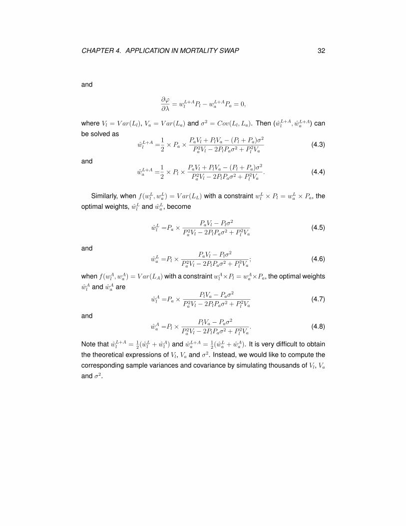
where Vl = V ar(Ll), Va = V ar(La) and σ2 = Cov(Ll, La). Then (wL+Al , wL+A
a ) can
be solved as
wL+Al =
1
2× Pa × PaVl + PlVa − (Pl + Pa)σ
2
P 2aVl − 2PlPaσ2 + P 2
l Va
(4.3)
and
wL+Aa =
1
2× Pl × PaVl + PlVa − (Pl + Pa)σ
2
P 2aVl − 2PlPaσ2 + P 2
l Va
. (4.4)
Similarly, when f(wLl , w
La ) = V ar(LL) with a constraint wL
l × Pl = wLa × Pa, the
optimal weights, wLl and wL
a , become
wLl =Pa × PaVl − Plσ
2
P 2aVl − 2PlPaσ2 + P 2
l Va
(4.5)
and
wLa =Pl × PaVl − Plσ
2
P 2aVl − 2PlPaσ2 + P 2
l Va
; (4.6)
when f(wAl , w
Aa ) = V ar(LA) with a constraint wA
l ×Pl = wAa ×Pa, the optimal weights
wAl and wA
a are
wAl =Pa × PlVa − Paσ
2
P 2aVl − 2PlPaσ2 + P 2
l Va
(4.7)
and
wAa =Pl × PlVa − Paσ
2
P 2aVl − 2PlPaσ2 + P 2
l Va
. (4.8)
Note that wL+Al = 1
2(wL
l + wAl ) and wL+A
a = 12(wL
a + wAa ). It is very difficult to obtain
the theoretical expressions of Vl, Va and σ2. Instead, we would like to compute the
corresponding sample variances and covariance by simulating thousands of Vl, Va
and σ2.
CHAPTER 4. APPLICATION IN MORTALITY SWAP 33
4.2 Numerical illustrations
4.2.1 Assumptions and portfolios
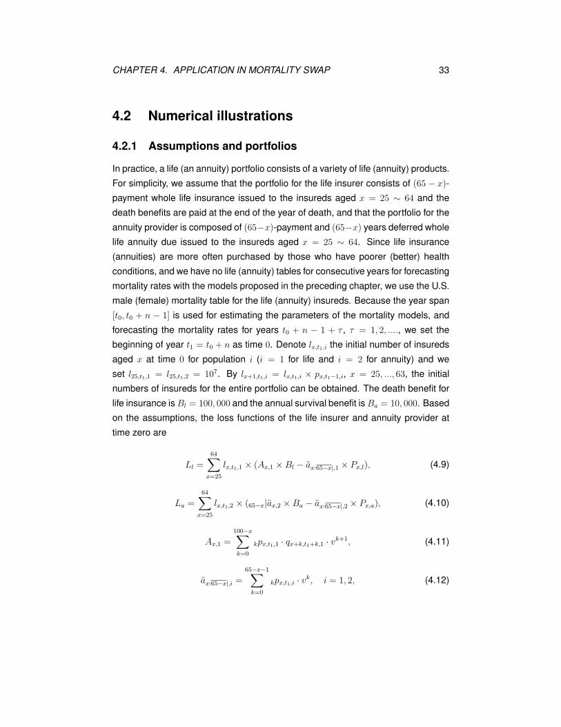
In practice, a life (an annuity) portfolio consists of a variety of life (annuity) products.
For simplicity, we assume that the portfolio for the life insurer consists of (65 − x)-
payment whole life insurance issued to the insureds aged x = 25 ∼ 64 and the
death benefits are paid at the end of the year of death, and that the portfolio for the
annuity provider is composed of (65−x)-payment and (65−x) years deferred whole
life annuity due issued to the insureds aged x = 25 ∼ 64. Since life insurance
(annuities) are more often purchased by those who have poorer (better) health
conditions, and we have no life (annuity) tables for consecutive years for forecasting
mortality rates with the models proposed in the preceding chapter, we use the U.S.
male (female) mortality table for the life (annuity) insureds. Because the year span
[t0, t0 + n − 1] is used for estimating the parameters of the mortality models, and
forecasting the mortality rates for years t0 + n − 1 + τ , τ = 1, 2, ...., we set the
beginning of year t1 = t0 + n as time 0. Denote lx,t1,i the initial number of insureds
aged x at time 0 for population i (i = 1 for life and i = 2 for annuity) and we
set l25,t1,1 = l25,t1,2 = 107. By lx+1,t1,i = lx,t1,i × px,t1−1,i, x = 25, ..., 63, the initial
numbers of insureds for the entire portfolio can be obtained. The death benefit for
life insurance is Bl = 100, 000 and the annual survival benefit is Ba = 10, 000. Based
on the assumptions, the loss functions of the life insurer and annuity provider at
time zero are
Ll =64∑
x=25
lx,t1,1 × (Ax,1 × Bl − ax:65−x|,1 × Px,l), (4.9)
La =64∑
x=25
lx,t1,2 × (65−x|ax,2 × Ba − ax:65−x|,2 × Px,a), (4.10)
Ax,1 =100−x∑
k=0
kpx,t1,1 · qx+k,t1+k,1 · vk+1, (4.11)
ax:65−x|,i =65−x−1∑
k=0
kpx,t1,i · vk, i = 1, 2, (4.12)

CHAPTER 4. APPLICATION IN MORTALITY SWAP 34
65−x|ax,2 =100∑
k=65
(k−x)px,t1,2 · vk−x, (4.13)
Px,l =Ax,1 × Bl
ax:65−x|,1, (4.14)
andPx,a =
65−x|ax,2 × Ba
ax:65−x|,2, (4.15)
where kpx,t1,i =∏k−1
j=0 px+j,t1+j,i with 0px,t1,i = 1, v = (1 + i)−1 and i = 6% is the
interest rate. Note that we set the limiting age equal to 100 for both populations, that
is, q100,t,i = 1, i = 1, 2. Moreover, Pl and Pa, the total present values of the future
premiums for the life insurer and annuity provider, respectively, in (4.3) ∼ (4.8) are
(see (4.9) and (4.10))
Pl =64∑
x=25
lx,t1,1 × ax:65−x|,1 × Px,l
and
Pa =64∑
x=25
lx,t1,2 × ax:65−x|,2 × Px,a.
The premiums Px,l and Px,a in (4.14) and (4.15), and the total premiums Pl and Pa
are pre-determined and do not respond to a change in mortality rates, whereas
Ax,1, ax:65−x|,i and 65−x|ax,2 in (4.11), (4.12) and (4.13) vary in response to the
realized mortality rates. Therefore, the deterministic mortality rates, qx,t0+n−1+τ ,
τ = 1, 2, ..., are used to calculate the premiums Px,l and Pa,x, and the stochastic
ones, qx,t0+n−1+τ , τ = 1, 2, ..., are used for simulations to compute Ax,1, ax:65−x|,i and
65−x|ax,2. When the realized mortality rates are different from the expected ones,
each of the loss functions Ll and La is either positive or negative. To forecast de-
terministic and stochastic mortality rates for ages 25 ∼ 64 and years 2011 ∼ 2086
using the four models given in Chapter 3, we set the year span [1981, 2010] and age
span [25, 100] (see Figure 4.4) to estimate the parameters with the male and female
mortality data from the Human Mortality Database for the life and annuity policies,
respectively. Specifically, for the independent model, we give the following steps to
forecast deterministic mortality rates for computing the premiums Px,l and Px,a:

CHAPTER 4. APPLICATION IN MORTALITY SWAP 35
Figure 4.4: age span [25, 100] and year span [1981, 2010]
1. compute ln(mx,2010+τ,i) = ax,i + bx,i × (k2010,i + τ × θi), i = 1, 2, τ = 1, 2, ..., 76,
x = 25, ..., 64;
2. transfer ln(mx,2010+τ,i) to qx,2010+τ,i; and
3. take the diagonal entries qx+τ−1,2010+τ,i, i = 1, 2, x = 25, ..., 64, τ = 1, 2, ..., (101−x).
To generate stochastic mortality rates for simulating Ax,1, ax:65−x|,i and 65−x|ax,2, a
similar procedure is given as follows:
1. generate sε,τ,i from N(0, 1) and sε,τ,i from N(0, 1), i = 1, 2, τ = 1, 2, ..., 76;
2. multiply sε,τ,i by σε,i, and sε,τ,i by σεx,i such that sε,τ,i × σε,i ∼ N(0, σ2ε,i) and
sε,τ,i × σεx,i ∼ N(0, σ2εx,i);
3. get simulated ln(mx,2010+τ,i) = ln(mx,2010+τ,i)+√τ×bx,i×sε,τ,i×σε,i+sε,τ,i×σεx,i,
i = 1, 2, τ = 1, 2, ..., 76, x = 25, ..., 64;
4. transfer ln(mx,2010+τ,i) to qx,2010+τ,i;
5. take the diagonal entries qx+τ−1,2010+τ,i, i = 1, 2, x = 25, ..., 64, τ = 1, 2, ..., (101−x); and
6. repeat steps (1) ∼ (5) for N times (N = 1, 000 in this project).
CHAPTER 4. APPLICATION IN MORTALITY SWAP 36
The procedures of forecasting the deterministic and stochastic mortality rates
for the joint-k, the co-integrated and the augmented common factor models are
similar to those above. With {qx+τ−1,2010+τ,i : i = 1, 2, x = 25, ..., 64, τ = 1, ..., (101−x)} and N {qx+τ−1,2010+τ,i : i = 1, 2, x = 25, ..., 64, τ = 1, ..., (101 − x)}’s, we can
calculate N realized values of Ll and La, get the sample variances Vl and Va and
the sample covariance σ2, and obtain the optimal weights with (4.3) ∼ (4.8).
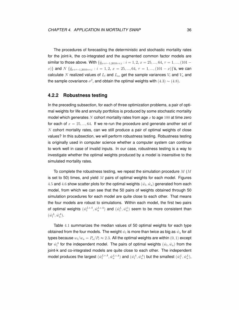
4.2.2 Robustness testing
In the preceding subsection, for each of three optimization problems, a pair of opti-
mal weights for life and annuity portfolios is produced by some stochastic mortality
model which generates N cohort mortality rates from age x to age 100 at time zero
for each of x = 25, ..., 64. If we re-run the procedure and generate another set of
N cohort mortality rates, can we still produce a pair of optimal weights of close
values? In this subsection, we will perform robustness testing. Robustness testing
is originally used in computer science whether a computer system can continue
to work well in case of invalid inputs. In our case, robustness testing is a way to
investigate whether the optimal weights produced by a model is insensitive to the
simulated mortality rates.
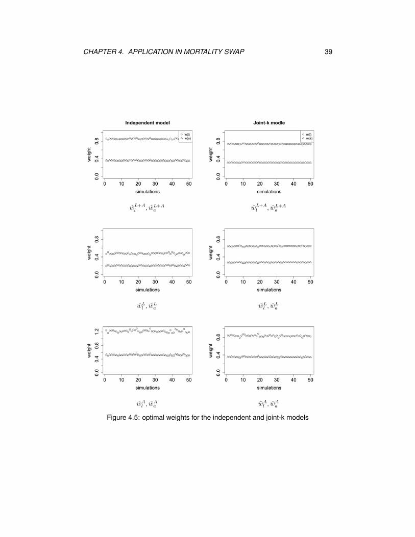
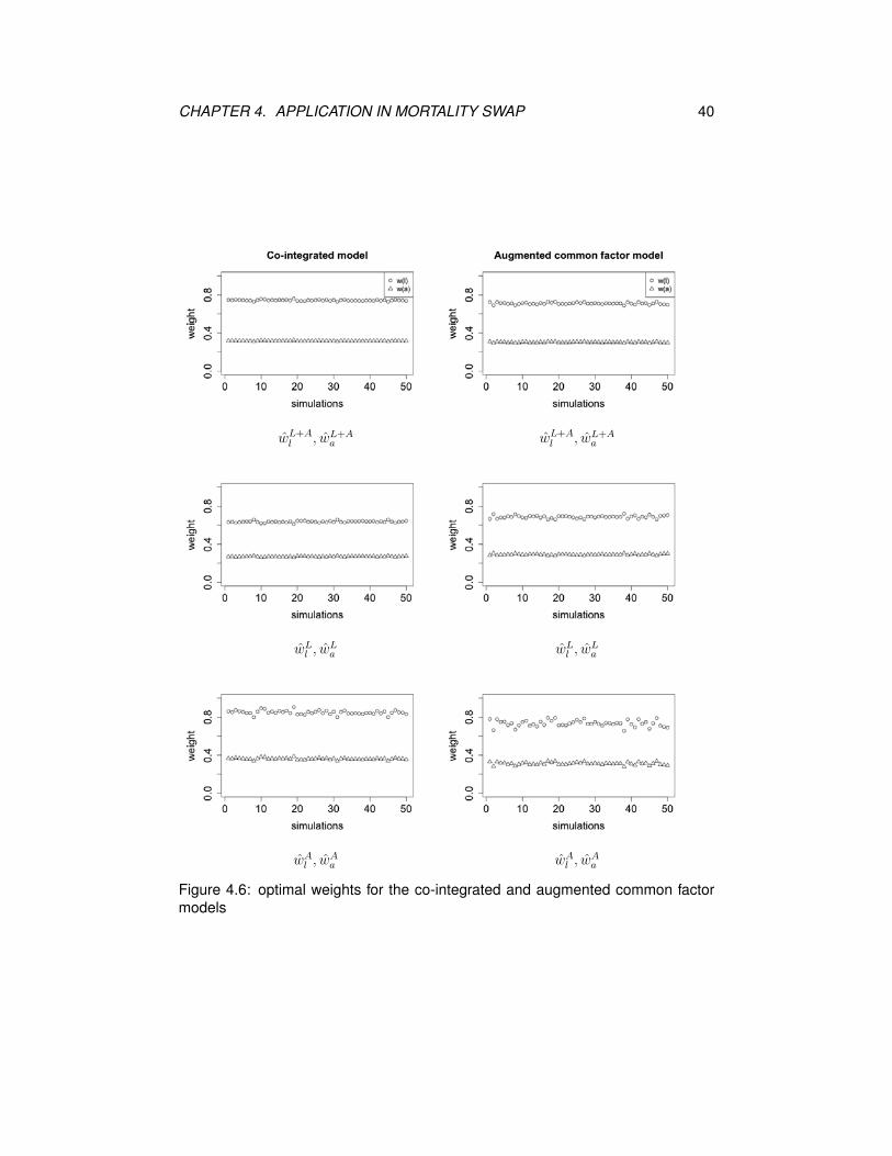
To complete the robustness testing, we repeat the simulation procedure M (M
is set to 50) times, and yield M pairs of optimal weights for each model. Figures
4.5 and 4.6 show scatter plots for the optimal weights (wl, wa) generated from each
model, from which we can see that the 50 pairs of weights obtained through 50
simulation procedures for each model are quite close to each other. That means
the four models are robust to simulations. Within each model, the first two pairs
of optimal weights (wL+Al , wL+A
a ) and (wLl , w
La ) seem to be more consistent than
(wAl , w
Aa ).
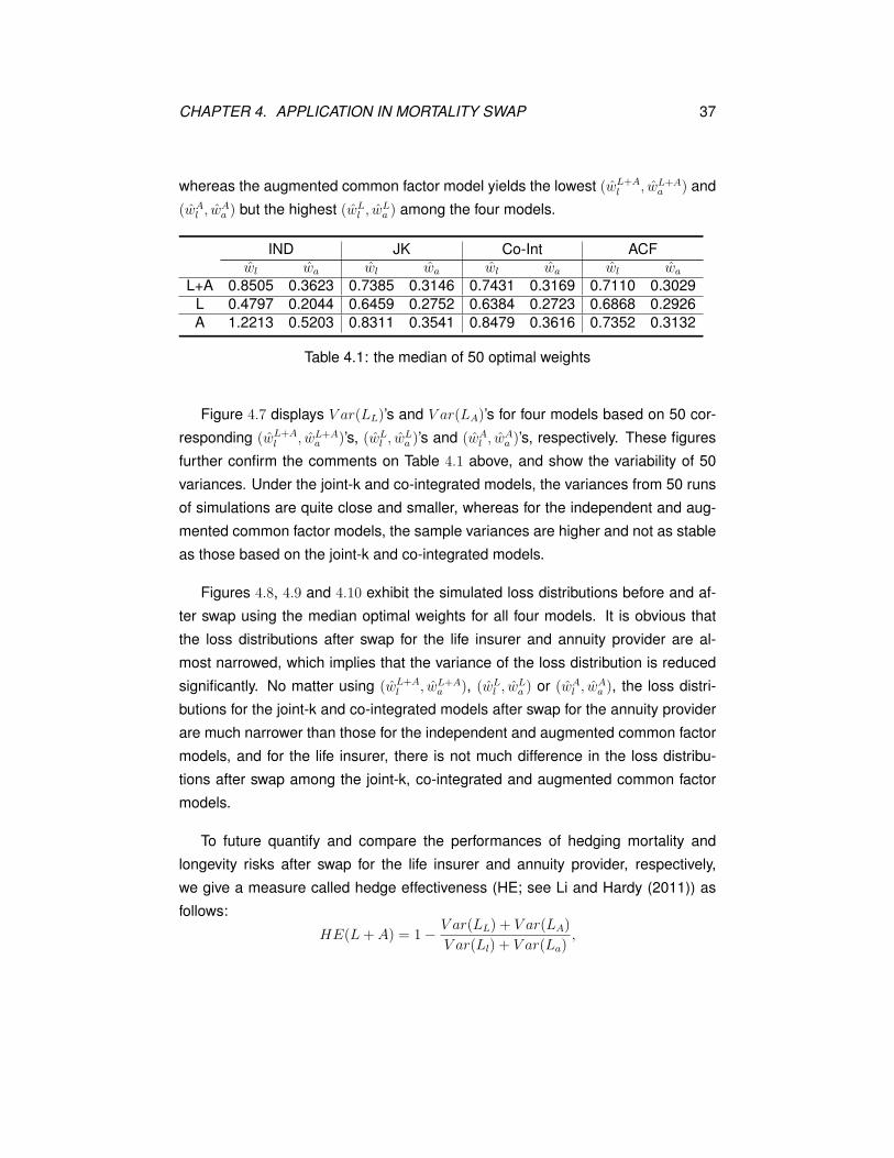
Table 4.1 summarizes the median values of 50 optimal weights for each type
obtained from the four models. The weight wl is more than twice as big as wa for all
types because wl/wa = Pa/Pl ≈ 2.3. All the optimal weights are within (0, 1) except
for wAl for the independent model. The pairs of optimal weights (wl, wa) from the
joint-k and co-integrated models are quite close to each other. The independent
model produces the largest (wL+Al , wL+A
a ) and (wAl , w
Aa ) but the smallest (wL
l , wLa ),
CHAPTER 4. APPLICATION IN MORTALITY SWAP 37
whereas the augmented common factor model yields the lowest (wL+Al , wL+A
a ) and
(wAl , w
Aa ) but the highest (wL
l , wLa ) among the four models.
IND JK Co-Int ACFwl wa wl wa wl wa wl wa
L+A 0.8505 0.3623 0.7385 0.3146 0.7431 0.3169 0.7110 0.3029L 0.4797 0.2044 0.6459 0.2752 0.6384 0.2723 0.6868 0.2926A 1.2213 0.5203 0.8311 0.3541 0.8479 0.3616 0.7352 0.3132
Table 4.1: the median of 50 optimal weights
Figure 4.7 displays V ar(LL)’s and V ar(LA)’s for four models based on 50 cor-
responding (wL+Al , wL+A
a )’s, (wLl , w
La )’s and (wA
l , wAa )’s, respectively. These figures
further confirm the comments on Table 4.1 above, and show the variability of 50
variances. Under the joint-k and co-integrated models, the variances from 50 runs
of simulations are quite close and smaller, whereas for the independent and aug-
mented common factor models, the sample variances are higher and not as stable
as those based on the joint-k and co-integrated models.
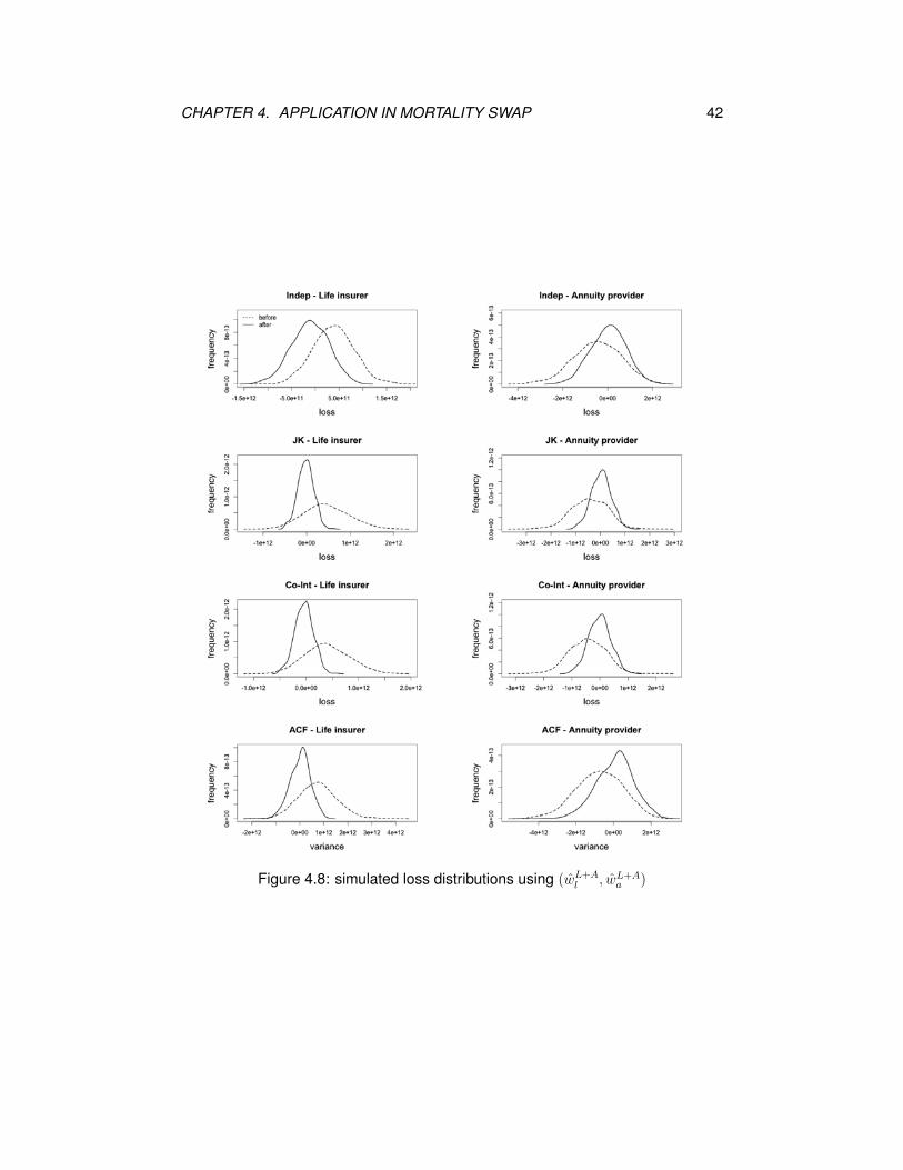
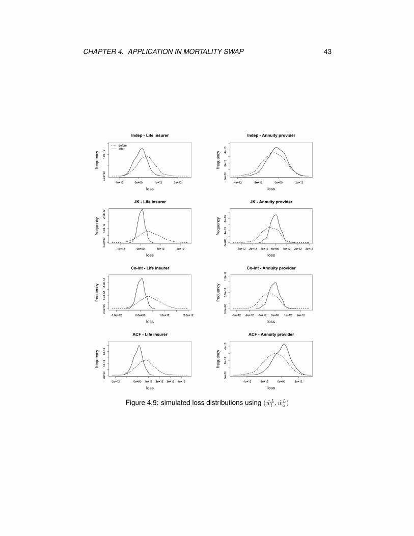
Figures 4.8, 4.9 and 4.10 exhibit the simulated loss distributions before and af-
ter swap using the median optimal weights for all four models. It is obvious that
the loss distributions after swap for the life insurer and annuity provider are al-
most narrowed, which implies that the variance of the loss distribution is reduced
significantly. No matter using (wL+Al , wL+A
a ), (wLl , w
La ) or (wA
l , wAa ), the loss distri-
butions for the joint-k and co-integrated models after swap for the annuity provider
are much narrower than those for the independent and augmented common factor
models, and for the life insurer, there is not much difference in the loss distribu-
tions after swap among the joint-k, co-integrated and augmented common factor
models.
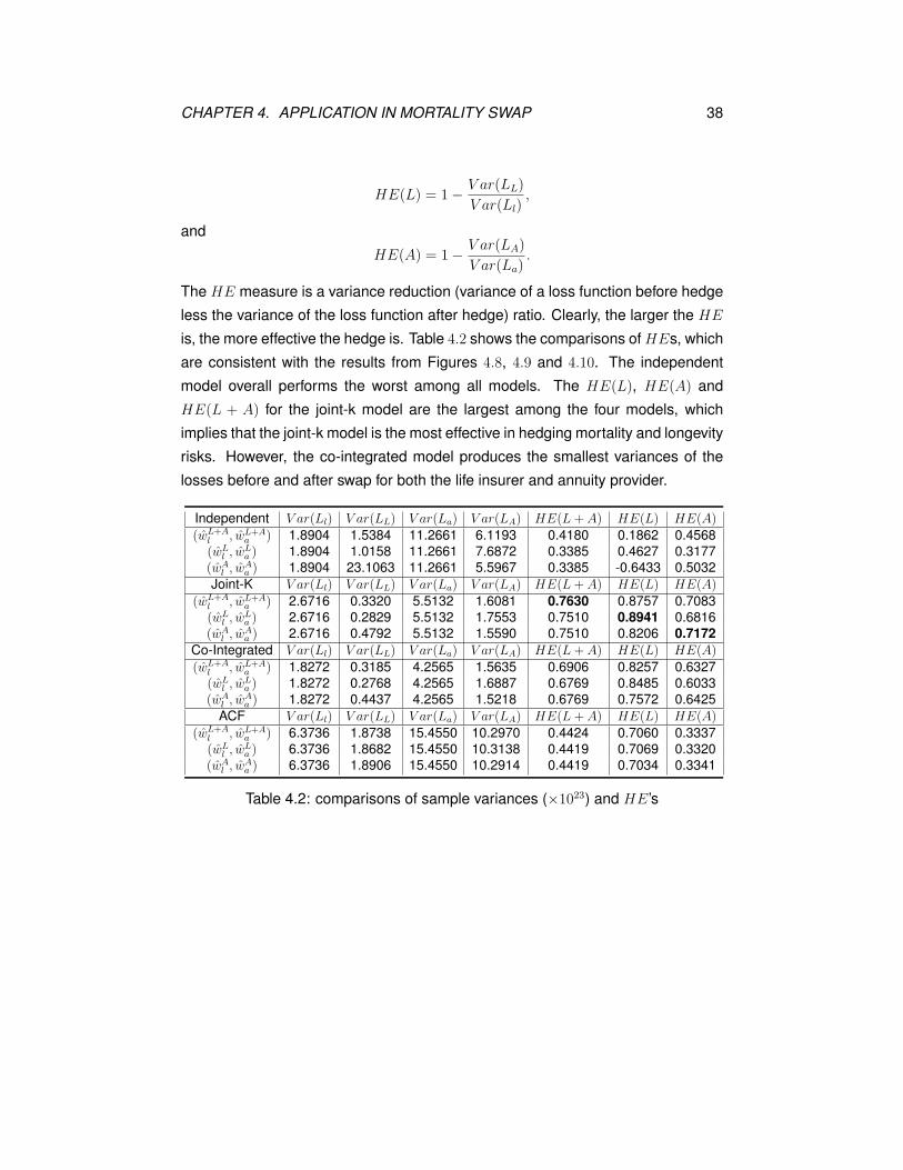
To future quantify and compare the performances of hedging mortality and
longevity risks after swap for the life insurer and annuity provider, respectively,
we give a measure called hedge effectiveness (HE; see Li and Hardy (2011)) as
follows:
HE(L+ A) = 1− V ar(LL) + V ar(LA)
V ar(Ll) + V ar(La),
CHAPTER 4. APPLICATION IN MORTALITY SWAP 38
HE(L) = 1− V ar(LL)
V ar(Ll),
and
HE(A) = 1− V ar(LA)
V ar(La).
The HE measure is a variance reduction (variance of a loss function before hedge
less the variance of the loss function after hedge) ratio. Clearly, the larger the HE
is, the more effective the hedge is. Table 4.2 shows the comparisons of HEs, which
are consistent with the results from Figures 4.8, 4.9 and 4.10. The independent
model overall performs the worst among all models. The HE(L), HE(A) and
HE(L + A) for the joint-k model are the largest among the four models, which
implies that the joint-k model is the most effective in hedging mortality and longevity
risks. However, the co-integrated model produces the smallest variances of the
losses before and after swap for both the life insurer and annuity provider.
Independent V ar(Ll) V ar(LL) V ar(La) V ar(LA) HE(L+ A) HE(L) HE(A)
(wL+Al , wL+A
a ) 1.8904 1.5384 11.2661 6.1193 0.4180 0.1862 0.4568(wL
l , wLa ) 1.8904 1.0158 11.2661 7.6872 0.3385 0.4627 0.3177
(wAl , w
Aa ) 1.8904 23.1063 11.2661 5.5967 0.3385 -0.6433 0.5032
Joint-K V ar(Ll) V ar(LL) V ar(La) V ar(LA) HE(L+ A) HE(L) HE(A)
(wL+Al , wL+A
a ) 2.6716 0.3320 5.5132 1.6081 0.7630 0.8757 0.7083(wL
l , wLa ) 2.6716 0.2829 5.5132 1.7553 0.7510 0.8941 0.6816
(wAl , w
Aa ) 2.6716 0.4792 5.5132 1.5590 0.7510 0.8206 0.7172
Co-Integrated V ar(Ll) V ar(LL) V ar(La) V ar(LA) HE(L+ A) HE(L) HE(A)
(wL+Al , wL+A
a ) 1.8272 0.3185 4.2565 1.5635 0.6906 0.8257 0.6327(wL
l , wLa ) 1.8272 0.2768 4.2565 1.6887 0.6769 0.8485 0.6033
(wAl , w
Aa ) 1.8272 0.4437 4.2565 1.5218 0.6769 0.7572 0.6425
ACF V ar(Ll) V ar(LL) V ar(La) V ar(LA) HE(L+ A) HE(L) HE(A)
(wL+Al , wL+A
a ) 6.3736 1.8738 15.4550 10.2970 0.4424 0.7060 0.3337(wL
l , wLa ) 6.3736 1.8682 15.4550 10.3138 0.4419 0.7069 0.3320
(wAl , w
Aa ) 6.3736 1.8906 15.4550 10.2914 0.4419 0.7034 0.3341
Table 4.2: comparisons of sample variances (×1023) and HE’s
CHAPTER 4. APPLICATION IN MORTALITY SWAP 39
wL+Al , wL+A
a wL+Al , wL+A
a
wLl , w
La wL
l , wLa
wAl , w
Aa wA
l , wAa
Figure 4.5: optimal weights for the independent and joint-k models
CHAPTER 4. APPLICATION IN MORTALITY SWAP 40
wL+Al , wL+A
a wL+Al , wL+A
a
wLl , w
La wL
l , wLa
wAl , w
Aa wA
l , wAa
Figure 4.6: optimal weights for the co-integrated and augmented common factormodels

CHAPTER 4. APPLICATION IN MORTALITY SWAP 41
V ar(LL)
variances using (wL+Al , wL+A
a )
V ar(LA)
variances using (wL+Al , wL+A
a )
variances using (wLl , w
La ) variances using (wL
l , wLa )
variances using (wAl , w
Aa ) variances using (wA
l , wAa )
Figure 4.7: variances after swap
CHAPTER 4. APPLICATION IN MORTALITY SWAP 42
Figure 4.8: simulated loss distributions using (wL+Al , wL+A
a )
CHAPTER 4. APPLICATION IN MORTALITY SWAP 43
Figure 4.9: simulated loss distributions using (wLl , w
La )

CHAPTER 4. APPLICATION IN MORTALITY SWAP 44
Figure 4.10: simulated loss distributions using (wAl , w
Aa )

Chapter 5
Block Bootstrap Method
In the preceding chapter, we forecast deterministic and stochastic mortality rates
with some two-population mortality models to determine the premiums of life and
annuity products and simulate the loss functions of portfolios of life and annuity
business. The weights of business for swap are calculated by the sample variances
and the sample covariance of the loss functions of the life insurer and annuity
provider before swap, which can minimize the risk of the portfolio and produce
high hedge effectiveness. All the great results are based on that the assumed
mortality model is the actual one, which, however, might not be true. Therefore,
both the life insurer and annuity provider face model risk and parameter risk that
will potentially affect the results. In this chapter, a bootstrap method which is model
and parameter free will be applied to generating samples for the future mortality
rates to calculate the weighted loss functions and their variances with the weights
obtained by each of the four models in Chapter 3.
Bootstrap is usually used to resample data with replacement to estimate some
statistic of a population from the sampled data. The procedure of the bootstrap
(naive bootstrap) is as follows:
1. Draw values from the original data set with replacement to form a new data
set of size n∗.
2. Repeat the first step N∗ times to obtain N∗ new data sets.
3. Compute the test statistic using the new data sets.
45

CHAPTER 5. BLOCK BOOTSTRAP METHOD 46
However, the naive bootstrap fails when applied to the mortality rates. First of
all, mortality rates over years can be treated as a time series displaying a decreas-
ing trend because of the improvement of medical and environmental conditions,
which shows mortality rates are not stationary. Secondly, the naive bootstrap is
likely to destroy the dependency of mortality rates on both age and time dimen-
sions. Alternatively, the block bootstrap can solve the problems above. First, re-
garding the non-stationary problem, differencing is a popular and effective method
of removing trend from a time series and making the time series weakly stationary.
The procedure is given below.
• Convert the empirical mortality rates qx,t,i to ln(mx,t,i), i = 1, 2, x = 25, ..., 100,
t = 1981, ..., 2009.
• Devide ln(mx,t+1,i) by ln(mx,t,i) to get the ratio, denoted by rx,t,i, that is, rx,t,i =ln(mx,t+1,i)
ln(mx,t,i), t = 1981, ..., 2009.
• Subtract rx,t,i from rx,t+1,i to get the difference, denoted by dx,t,i, that is, dx,t,i =
rx,t+1,i − rx,t,i, t = 1981, ..., 2008.
Figure 5.1 shows the time series {dx,t,i}, i = 1, 2, for the U.S. males and females
aged 35, 45, 55 and 65, which look stationary.

CHAPTER 5. BLOCK BOOTSTRAP METHOD 47
Figure 5.1: {dx,t,i} for x = 35, 45, 55, 65
CHAPTER 5. BLOCK BOOTSTRAP METHOD 48
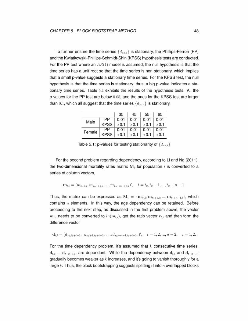
To further ensure the time series {dx,t,i} is stationary, the Phillips-Perron (PP)
and the Kwiatkowski-Phillips-Schmidt-Shin (KPSS) hypothesis tests are conducted.
For the PP test where an AR(1) model is assumed, the null hypothesis is that the
time series has a unit root so that the time series is non-stationary, which implies
that a small p-value suggests a stationary time series. For the KPSS test, the null
hypothesis is that the time series is stationary; thus, a big p-value indicates a sta-
tionary time series. Table 5.1 exhibits the results of the hypothesis tests. All the
p-values for the PP test are below 0.05, and the ones for the KPSS test are larger
than 0.1, which all suggest that the time series {dx,t,i} is stationary.
35 45 55 65
Male PP 0.01 0.01 0.01 0.01KPSS >0.1 >0.1 >0.1 >0.1
Female PP 0.01 0.01 0.01 0.01KPSS >0.1 >0.1 >0.1 >0.1
Table 5.1: p-values for testing stationarity of {dx,t,i}
For the second problem regarding dependency, according to Li and Ng (2011),
the two-dimensional mortality rates matrix Mi for population i is converted to a
series of column vectors,
mt,i = (mx0,t,i,mx0+1,t,i, ...,mx0+m−1,t,i)′, t = t0, t0 + 1, ..., t0 + n− 1.
Thus, the matrix can be expressed as Mi = {mt0,i,mt0+1,i, ...,mt0+n−1,i}, which
contains n elements. In this way, the age dependency can be retained. Before
proceeding to the next step, as discussed in the first problem above, the vector
mt,i needs to be converted to ln(mt,i), get the ratio vector rt,i and then form the
difference vector
dt,i = (dx0,t0+t−1,i, dx0+1,t0+t−1,i, ..., dx0+m−1,t0+t−1,i)′, t = 1, 2, ..., n− 2, i = 1, 2.
For the time dependency problem, it’s assumed that k consecutive time series,
dt,i, ...,dt+k−1,i, are dependent. While the dependency between dt,i and dt+k−1,i
gradually becomes weaker as k increases, and it’s going to vanish thoroughly for a
large k. Thus, the block bootstrapping suggests splitting d into n overlapped blocks
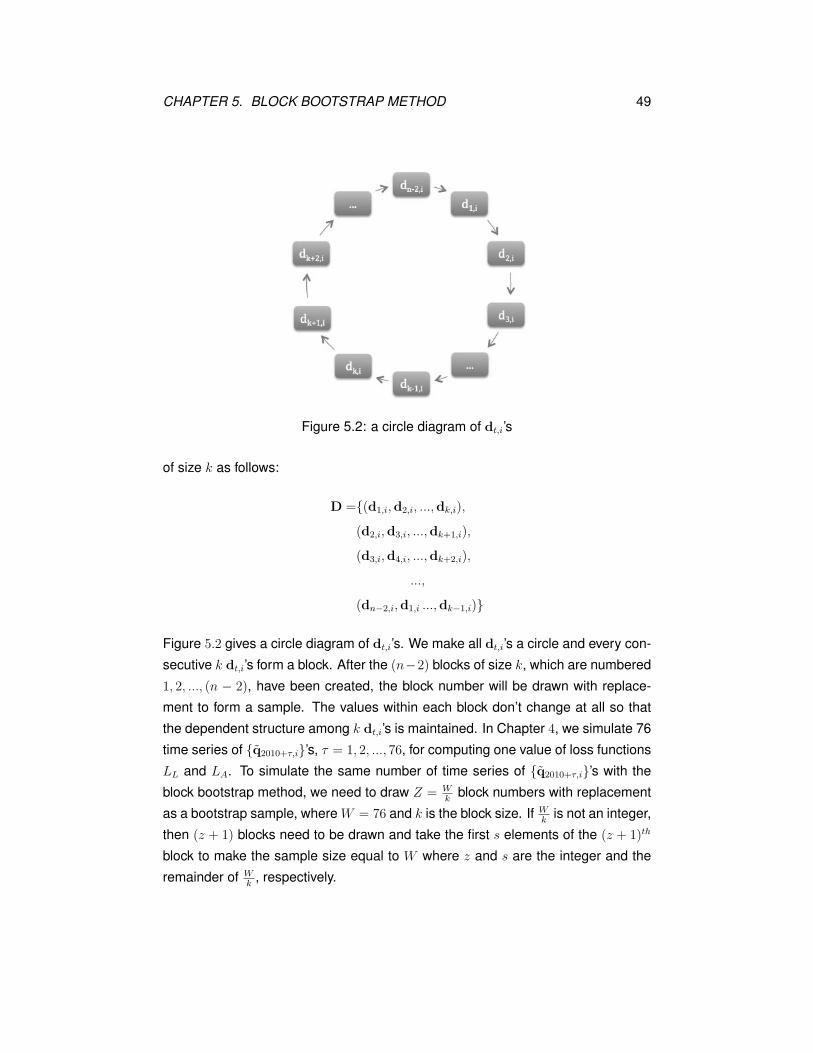
CHAPTER 5. BLOCK BOOTSTRAP METHOD 49
Figure 5.2: a circle diagram of dt,i’s
of size k as follows:
D ={(d1,i,d2,i, ...,dk,i),
(d2,i,d3,i, ...,dk+1,i),
(d3,i,d4,i, ...,dk+2,i),
...,
(dn−2,i,d1,i ...,dk−1,i)}
Figure 5.2 gives a circle diagram of dt,i’s. We make all dt,i’s a circle and every con-
secutive k dt,i’s form a block. After the (n−2) blocks of size k, which are numbered
1, 2, ..., (n − 2), have been created, the block number will be drawn with replace-
ment to form a sample. The values within each block don’t change at all so that
the dependent structure among k dt,i’s is maintained. In Chapter 4, we simulate 76
time series of {q2010+τ,i}’s, τ = 1, 2, ..., 76, for computing one value of loss functions
LL and LA. To simulate the same number of time series of {q2010+τ,i}’s with the
block bootstrap method, we need to draw Z = Wk
block numbers with replacement
as a bootstrap sample, where W = 76 and k is the block size. If Wk
is not an integer,
then (z + 1) blocks need to be drawn and take the first s elements of the (z + 1)th
block to make the sample size equal to W where z and s are the integer and the
remainder of Wk
, respectively.

CHAPTER 5. BLOCK BOOTSTRAP METHOD 50
Finally, the block size is determined by the size of observations V . As sug-
gested by Hall et al. (1995), the optimal block size, k, can be V13 , V
14 or V
15 . Since
there are 28 {dt,i}’s (V = n− 2 = 28), a block size of 2 is chosen.
The following is the procedure of the block bootstrap method.
1. Take the logarithm on the real central death rates, ln(mx,t,i), for i = 1, 2,
x = x0, ..., x0 +m− 1, and t = t0, ..., t0 + n− 1.
2. Get rx,t,i =ln(mx,t+1,i)
ln(mx,t,i)and dx,t,i = rx,t+1,i − rx,t,i.
3. Form column vector dt,i = (dx0,t0+t−1,i, dx0+1,t0+t−1,i, ..., dx0+m−1,t0+t−1,i)′, t =
1, ..., n− 2.
4. Form the jth block of size 2, (dj,i,dj+1,i), j = 1, ..., n − 3, and the (n − 2)th
block, (dn−2,i,d1,i).
5. Draw a bootstrap sample of size Z = W2
if W is even, or Z = (W+1)2
if W is
odd to get the block numbers b1, b2,..., bZ (all the indices fall between 1 and
n− 2).
6. Get the indices, b1, b1 +1, b2, b2 +1,..., bZ , bZ +1 if W is even, or b1, b1 +1, b2,
b2 +1,..., bZ if W is odd; if bj = n− 2 for some j, then assign index 1 to bj +1.
Denote the jth index as cj, j = 1, ...,W .
7. Obtain the column vector dcj ,i = (dx0,t0+cj−1,i, ..., dx0+m−1,t0+cj−1,i)′, j = 1, ...,W .
8. Obtain simulated mx,t0+n−1+τ,i by
mx,t0+n−1+τ,i = exp{ln(mx,t0+n−1+τ−1,i)× [ln(mx,t0+n−1,i)
ln(mx,t0+n−2,i)+
τ∑
j=1
dx,t0+cj−1,i]},
i = 1, 2, τ = 1, 2, ..., 76, x = x0, x0 + 1, ..., x0 +m− 1.
9. Convert simulated mx,t0+n−1+τ,i matrix to qx,t0+n−1+τ,i matrix and take the di-
agonal entries to form cohort mortality sequences.
10. Repeat (3)-(9) for N times (N = 1000).
CHAPTER 5. BLOCK BOOTSTRAP METHOD 51
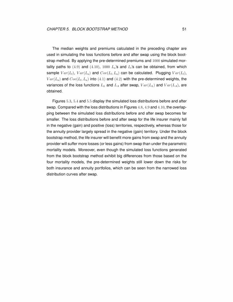
The median weights and premiums calculated in the preceding chapter are
used in simulating the loss functions before and after swap using the block boot-
strap method. By applying the pre-determined premiums and 1000 simulated mor-
tality paths to (4.9) and (4.10), 1000 La’s and Ll’s can be obtained, from which
sample V ar(Ll), V ar(La) and Cov(Ll, La) can be calculated. Plugging V ar(Ll),
V ar(La) and Cov(Ll, La) into (4.1) and (4.2) with the pre-determined weights, the
variances of the loss functions LL and LA after swap, V ar(LL) and V ar(LA), are
obtained.
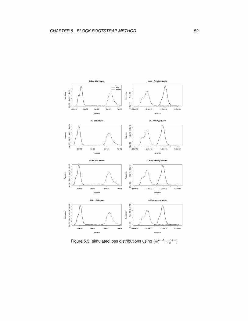
Figures 5.3, 5.4 and 5.5 display the simulated loss distributions before and after
swap. Compared with the loss distributions in Figures 4.8, 4.9 and 4.10, the overlap-
ping between the simulated loss distributions before and after swap becomes far
smaller. The loss distributions before and after swap for the life insurer mainly fall
in the negative (gain) and positive (loss) territories, respectively, whereas those for
the annuity provider largely spread in the negative (gain) territory. Under the block
bootstrap method, the life insurer will benefit more gains from swap and the annuity
provider will suffer more losses (or less gains) from swap than under the parametric
mortality models. Moreover, even though the simulated loss functions generated
from the block bootstrap method exhibit big differences from those based on the
four mortality models, the pre-determined weights still lower down the risks for
both insurance and annuity portfolios, which can be seen from the narrowed loss
distribution curves after swap.
CHAPTER 5. BLOCK BOOTSTRAP METHOD 52
Figure 5.3: simulated loss distributions using (wL+Al , wL+A
a )

CHAPTER 5. BLOCK BOOTSTRAP METHOD 53
Figure 5.4: simulated loss distributions using (wLl , w
La )
CHAPTER 5. BLOCK BOOTSTRAP METHOD 54
Figure 5.5: simulated loss distributions using (wAl , w
Aa )

CHAPTER 5. BLOCK BOOTSTRAP METHOD 55
Similar to Table 4.2, Table 5.2 shows the sample variances and hedge effec-
tiveness (HE) under the block bootstrap method. In this case, the differences
in HE and V ar(L) among four models are not as obvious as those using multi-
population mortality models because the same simulated mortality rates from the
block bootstrap method are applied to the loss functions before and after swap with
different (wl, wa)’s from four mortality models. Compared with the values in Table
4.2, the variances of the loss functions before and after swap for both life insurer
and annuity provider are far enlarged except for V ar(LL) based on (wAl , w
Aa ) for
the independent model. The HEs generally increase for the independent model,
and decrease for the joint-k and co-integrated models. Among the four models,
the co-integrated and independent models achieve the highest and the lowest
hedge effectiveness, respectively, for HE(L + A), HE(L) and HE(A) based on
(wL+Al , wL+A
a ), (wLl , w
La ) and (wA
l , wAa ), respectively. The joint-k model can also pro-
duce high hedge effectiveness. Thus, under model-free block bootstrap method,
the joint-k and co-integrated models still outperform the other two models.
Independent V ar(Ll) V ar(LL) V ar(La) V ar(LA) HE(L+ A) HE(L) HE(A)
(wL+Al , wL+A
a ) 12.1508 5.6147 43.0437 23.2084 0.4778 0.5379 0.4608(wL
l , wLa ) 12.1508 4.4826 43.0437 27.8747 0.4138 0.6311 0.3524
(wAl , w
Aa ) 12.1508 12.9029 43.0437 24.6982 0.3188 -0.0619 0.4262
Joint-K V ar(Ll) V ar(LL) V ar(La) V ar(LA) HE(L+ A) HE(L) HE(A)
(wL+Al , wL+A
a ) 12.1509 4.6247 43.0495 23.9732 0.4819 0.6194 0.4431(wL
l , wLa ) 12.1509 4.2296 43.0495 25.0259 0.4700 0.6519 0.4187
(wAl , w
Aa ) 12.1509 5.4035 43.0495 23.3042 0.4799 0.5553 0.4587
Co-Integrated V ar(Ll) V ar(LL) V ar(La) V ar(LA) HE(L+ A) HE(L) HE(A)
(wL+Al , wL+A
a ) 12.1508 4.6638 43.0511 23.9150 0.4823 0.6162 0.4445(wL
l , wLa ) 12.1508 4.2211 43.0511 25.1140 0.4686 0.6526 0.4166
(wAl , w
Aa ) 12.1508 5.5980 43.0511 23.2074 0.4782 0.5393 0.4782
ACF V ar(Ll) V ar(LL) V ar(La) V ar(LA) HE(L+ A) HE(L) HE(A)
(wL+Al , wL+A
a ) 12.1231 4.4638 43.0398 24.2210 0.4800 0.6318 0.4372(wL
l , wLa ) 12.1231 4.3527 43.0398 24.4902 0.4771 0.6410 0.4310
(wAl , w
Aa ) 12.1231 4.6011 43.0398 23.9780 0.4819 0.6205 0.4429
Table 5.2: comparisons of sample variances (×1023) and HE’s (block bootstrap)

Chapter 6
Conclusion
The strategy of natural hedging in this project shows a significant effect on reducing
risks of insurance and annuity portfolios by swapping business. The robustness
testing exhibits that the optimal weights and the variances of the loss functions after
swap for both life insurer and annuity provider obtained from four multi-population
models are robust to simulations.
The performances of hedging mortality and longevity risks for each model are
compared in two ways; one is based on parametric multi-population mortality mod-
els, and the other is based on non-parametric block bootstrap method. Both ways
suggest that the joint-k and co-integrated models outperform the independent and
augmented common factor models, which implies that the improvement on mortal-
ity rates between two populations tend to become more related, and assuming a
stronger bond between two time-varying factors for two populations seems to be
more reasonable when forecasting future mortality rates.
Although natural hedging can achieve the goal of reducing the variance of the
loss, future research can still be carried out so that it can be further applied to more
practical situations. For example, both a life insurer and an annuity provider won’t
swap their business directly in practice. Generally, companies prefer to transfer
their business to a financial intermediary called SPV (special purpose vehicle) who
is in charge of business swapping. Another problem is that the portfolio of life
(annuity) business in this project consists of only one type of life insurance (annuity)
product, the (65− x)-payment whole life insurance ((65− x)-payment and (65− x)
deferred whole life annuity due), which is too simple to be practical.
56

Bibliography
[1] D. Blake and W. Burrows. Survivor bonds: Helping to hedge mortality risk.Journal of Risk and Insurance, 68:339–348, 2001.
[2] N.L. Bowers, H.U. Gerber, J.C. Hickman, D.A. Jones, and C.J. Nesbitt. Actu-arial mathematics. 2nd ed. The Society of Actuaries, 1997.
[3] S.H. Cox and Y. Lin. Natural hedging of life and annuity mortality risks. NorthAmerican Actuarial Journal, 11:1–15, 2007.
[4] P. Gaillardetz, H.Y. Li, and A. MacKay. Equity-linked products: Evaluation ofthe dynamic hedging errors under stochastic mortality. European ActuarialJournal, 2:243–258, 2012.
[5] P. Hall, J.L. Horowitz, and B.Y. Jing. On blocking rules for the bootstrap withdependent data. Biometrika, 82:561–574, 1995.
[6] R.D. Lee and L.R. Carter. Modeling and forecasting U.S. mortality. Journal ofthe American Statistical Association, 87:659–671, 1992.
[7] J.S. Li and M.R. Hardy. Measuring basis risk in longevity hedges. NorthAmerican Actuarial Journal, 15:177–200, 2011.
[8] J.S. Li and A.C. Ng. Canonical valuation of mortality-linked securities. TheJournal of Risk and Insurance, 78:853–884, 2011.
[9] N. Li and R. Lee. Coherent mortality forecasts for a group of populations: Anextension of the Lee-Carter method. Demography, 42:575–594, 2005.
[10] T. Lin and C.C.L. Tsai. On the mortality/longevity risk hedging with mortalityimmunization. Insurance: Mathematics and Economics, 53:580–596, 2013.
[11] A. Milidonis, Y. Lin, and S.H. Cox. Mortality regimes and pricing. North Amer-ican Actuarial Journal, 15:266–289, 2011.
[12] J.L. Wang, H.C. Huang, S.S. Yang, and J.T. Tsai. An optimal product mix forhedging longevity risk in life insurance companies: The immunization theoryapproach. The Journal of Risk and Insurance, 77:473–497, 2010.
[13] N. Zhu and D. Bauer. A cautionary note on natural hedging of longevity risk.North American Actuarial Journal, 18:104–115, 2014.
57