NATURAL BOULDER EXPOSED TO THE SUN: A TEST OF …jmconrad/GradStudents/Thesis_Swami.pdf ·...
148
TEMPERATURE, STRAIN AND ACOUSTIC EMISSION MONITORING OF A NATURAL BOULDER EXPOSED TO THE SUN: A TEST OF THE EFFICACY OF INSOLATION ON PHYSICAL WEATHERING by Suraj G. Swami A thesis submitted to the faculty of The University of North Carolina at Charlotte in partial fulfillment of the requirements for the degree of Master of Science in Electrical Engineering Charlotte 2011 Approved by: ______________________________ Dr. James M. Conrad ______________________________ Dr. Kimberly A. Warren _____________________________ Dr. Martha C. Eppes ______________________________ Dr. Andrew R. Willis
Transcript of NATURAL BOULDER EXPOSED TO THE SUN: A TEST OF …jmconrad/GradStudents/Thesis_Swami.pdf ·...

TEMPERATURE, STRAIN AND ACOUSTIC EMISSION MONITORING OF A
NATURAL BOULDER EXPOSED TO THE SUN: A TEST OF THE EFFICACY OF
INSOLATION ON PHYSICAL WEATHERING
by
Suraj G. Swami
A thesis submitted to the faculty of
The University of North Carolina at Charlotte
in partial fulfillment of the requirements
for the degree of Master of Science in
Electrical Engineering
Charlotte
2011
Approved by:
______________________________
Dr. James M. Conrad
______________________________
Dr. Kimberly A. Warren
_____________________________
Dr. Martha C. Eppes
______________________________
Dr. Andrew R. Willis

ii
© 2011
Suraj G. Swami
ALL RIGHTS RESERVED

iii
ABSTRACT
SURAJ G. SWAMI. Temperature, strain and acoustic emission monitoring of a natural
boulder exposed to the sun: A test of the efficacy of insolation on physical weathering.
(Under the direction of DR. JAMES M. CONRAD, DR. KIMBERLY A. WARREN and
DR. MARTHA C. EPPES)
The efficacy of simple diurnal exposure in cracking rocks has been debated for
over a century. This instrumentation study is a continuation of the study conducted by
Garbini (2009) to correlate the diurnal formation of cracks in rock (as detected by
acoustic emissions (AE)) to surface strain, surface temperature, surface moisture, soil
moisture and ambient weather conditions for a period of seven months from June 20,
2010 to January 13, 2011. If thermal stresses related to insolation are responsible for rock
cracks, then both spatial and temporal correlations should be evident between AE events
and rock surface and environmental conditions. Data is recorded using two data loggers
and remotely collected using a wireless modem, powered using solar panels. During the
194 day observation period, 29,541 AE events occurred over a total of 902 minute
intervals during 68 days. Of the 29,451 events, 7,834 were “dry” AE events (no moisture
detected by the surface moisture sensor). In this study, data suggest that the cracks are
formed due to cyclic processes only when the cyclic stress exceeds the fatigue limit of the
rock. The majority of cracks are on the top part of the rock and on the south-east. A large
number of cracks are oriented along the north-south similar to McFadden et al. (2005),
Eppes et al. (2010). The data presented in this study provide further evidence of
insolation-related thermal stresses causing rocks to crack.

iv
ACKNOWLEDGEMENTS
This research has been funded by a grant from the National Science Foundation
(EAR Award #0844335) and supported by the Departments of Geography & Earth
Sciences and Civil and Environmental Engineering at UNC Charlotte.
It has been an exciting journey for the past two years I spent as a graduate student
at the University of North Carolina at Charlotte. A number of people have contributed in
assorted ways to this research and my experience here at UNC Charlotte. It is a pleasure
to convey my gratitude to them.
First and foremost, I would like to thank my advisors Dr. James M. Conrad, Dr.
Martha C. Eppes and Dr. Kimberly A. Warren for their supervision, advice and guidance
from the very early stage of this research. Their perpetual enthusiasm and constant
encouragement was the backbone of its success. It has been a privilege working with
them. I would also like to thank the members of my thesis committee, Dr. Andrew R.
Willis for valuable feedback.
I thank my family and friends for their love and support. I dedicate this thesis to
my father whose constant faith in me motivated me to stand where I am today.
v
TABLE OF CONTENTS
LIST OF FIGURES ix
LIST OF TABLES xiii
CHAPTER 1: INTRODUCTION 1
1.1 Research Motivation 1
1.2 Research Objectives 3
1.3 Research Scope 4
CHAPTER 2: LITERATURE REVIEW 5
2.1 Background 5
2.2 The influence of Rate of Temperature Change on physical weathering 7
2.3 Cyclic Processes leading to physical weathering by fatigue 9
2.4 Study on Location of cracks 11
2.5 Summary of Garbini (2009) 15
2.5.1 Instrumentation 15
2.5.2 Observations 16
2.6 Literature Review Summary 17
CHAPTER 3: INSTRUMENTATION 19
3.1 Test Specimen 20
3.2 Measurement of Strain 22
3.2.1 Strain Gage Selection 22
3.2.2 Strain Gage Installation 24
3.2.3 Strain Gage Location 28
3.2.4 Summary on Strain Gage Measurement 30

vi
3.3 Measurement of Surface Temperature 30
3.4 Measurement of Acoustic Emissions 32
3.4.1 Acoustic Emission Sensor Selection 34
3.4.2 AE Sensor Installation 34
3.4.3 Finding Wave Velocity 36
3.4.4 AE Sensor Location and Validation Test 37
3.5 Surface Moisture 45
3.6 Measurement of the Environmental Conditions 46
3.7 Soil Moisture 49
CHAPTER 4: DATA ACQUISITION AND ANALYSIS METHODS 51
4.1 Data Acquisition 53
4.1.1 CR1000 Data Acquisition System 53
4.1.2 Sensor Highway-II (SH-II) Data Acquisition System 54
4.2 Remote Connectivity Communication 55
4.3 Power 57
4.3.1 Battery Charge Controller 59
4.3.2 Field Deployment Process 61
4.4 Data Archival Procedure 64
4.4.1 CR1000 Data Archival 65
4.4.2 SH-II Data Archival 65
4.4.3 Merging CR1000 and SH-II Dataset 66
4.5 Data Analysis 67
4.5.1 Analysis using the Excel Spreadsheet Template 67
4.5.2 Analysis using MATLAB 70
vii
4.5.3 Data Analysis Summary 74
CHAPTER 5: RESULTS AND DISCUSSION 76
5.1 Test specimen conditions throughout the observation period 77
5.1.1 General trends in surface temperature and strain 77
5.1.2 Temperature differences across the test specimen 80
5.1.3 Rate of change of surface temperature 86
5.1.4 Strain exerted on the rock 89
5.1.5 Difference between ambient temperature and surface temperature 93
5.2 Event Analysis 94
5.2.1 Timing of Events 96
5.2.2 Influence of temperature on the formation of cracks 99
5.2.2.1 Surface Temperature of the rock concurrent with events 99
5.2.2.2 Temperature difference across the rock surface during events 101
5.2.2.3 Rate of change of test specimen temperature before events 106
5.2.2.4 Rate of change of maximum – minimum surface temperature 110
5.2.3 Effect of Weather on events 112
5.2.3.1 Rain 112
5.2.3.2 Insolation 117
5.2.3.3 Wind speed and wind direction 119
5.2.4 Event Location 121
5.3 Interpretation of results 122
5.3.1 Hypothesis 1 122
5.3.2 Hypothesis 2 123
5.3.3 Hypothesis 3 124

viii
5.3.4 Hypothesis 4 124
5.3.5 Hypothesis 5 125
5.3.6 Hypothesis 6 125
CHAPTER 6: SUMMARY 126
6.1 Project Summary 126
6.2 Goals achieved 127
6.3 Experimental observations 127
6.4 Future Work 129
REFERENCES 131

ix
LIST OF FIGURES
FIGURE 3.1: (a) Campbell Scientific CR1000 data acquisition system; 20
(b) Physical Acoustics Corporation Sensor Highway II data acquisition system
FIGURE 3.2: Granite boulder field specimen (a) west-facing side (profile view); 21
(b) east-facing side (profile view); (c) south-facing side (profile view); (d) north-
facing side (profile view); (e) obliquely from the top; (f) view of the dimple.
Directions refer to the pre-determined orientation of the boulder once placed in
the field
FIGURE 3.3: (a) Typical uniaxial foil strain gage; (b) rectangular rosette foil strain 23
gage
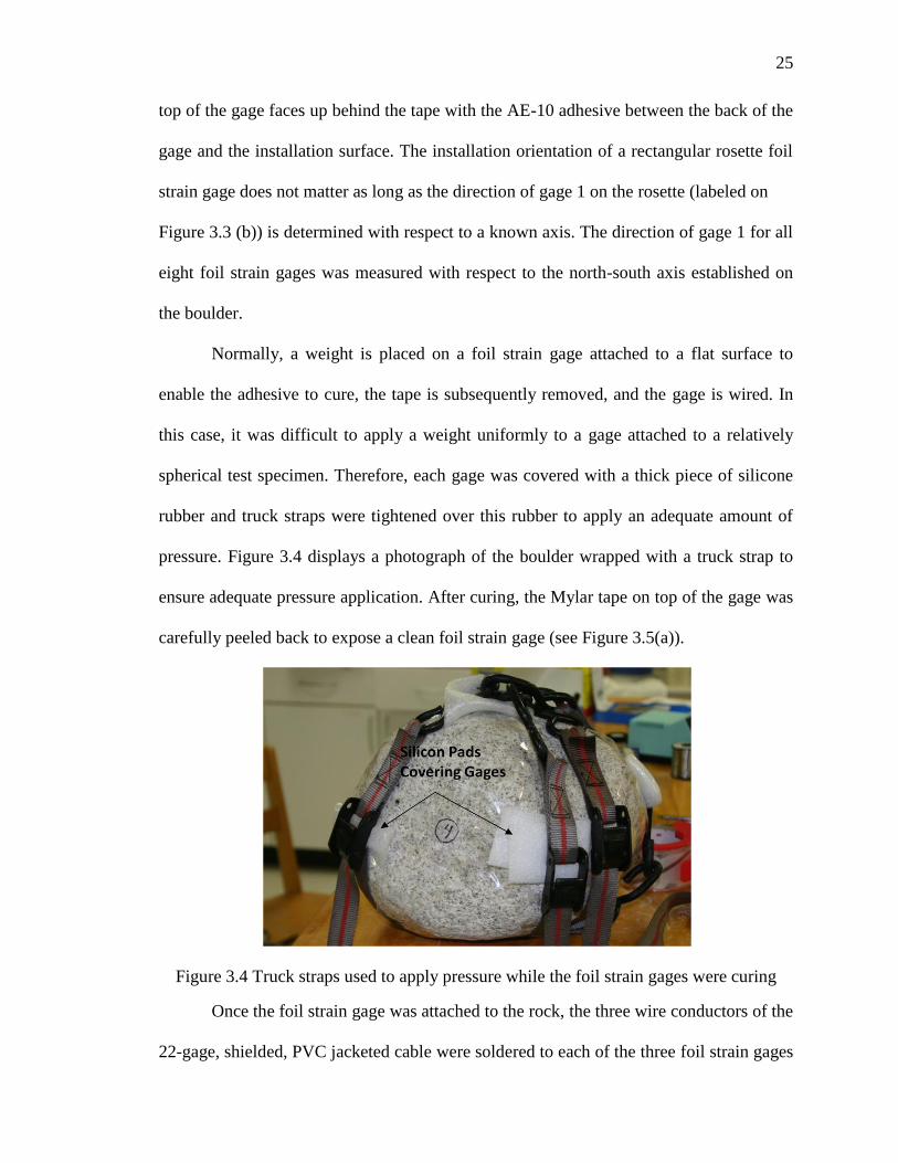
FIGURE 3.4: Truck straps used to apply pressure while the foil strain gages were 25
curing
FIGURE 3.5: Stages of preparation and wiring of a single rectangular rosette on the 27
rock surface: (a) Rectangular rosette and adjacent terminals; (b) foil strain gages
and terminals with solder dots on them in preparation for wiring; (c) single, tinned
terminal wire connecting foil strain gages to the terminals; (d) conductor wires
soldered to the terminals
FIGURE 3.6: Application of the foil strain gage protection: (a) Wired foil strain gage 28
taped for wax application; (b) layers of hot wax applied directly to the foil strain
gage; (c) clear silicone adhesive applied to the surface of the wax protection;
(d) foil strain gage with complete environmental protection
FIGURE 3.8: Thermocouple Installation: (a) cement adhesive used to attach all 31
thermocouples; (b) T-Type (copper-constantan) thermocouple; (c) T-Type
thermocouple installed on the surface of the boulder next to a protected strain
rosette
FIGURE 3.9: (a) Schematic of an acoustic emission sensor; (b) Physical Acoustics 33
Corporation acoustic emission sensor utilized during this study (PK151)
FIGURE 3.10: Acoustic emission sensors, foil strain gages, surface moisture sensor, 35
and thermocouples installed on the boulder
FIGURE 3.11: (a) Calibration block with acoustic emission sensors temporarily 38
attached with adhesive tape; (b) Pencil Lead Break Test performed on the
calibration block in accordance with ASTM E 976
FIGURE 3.12: Calibration block and AE sensors in AE Win software 39
FIGURE 3.13: Three sided box used to measure the x, y, and z coordinates on the 41
boulder
x
FIGURE 3.14: AE Sensor (numbered) location: Side View of the test specimen 42
( North-South )
FIGURE 3.15: AE Sensor (numbered) location: Side View of the test specimen 42
(West-East)
FIGURE 3.16 AE Sensor (numbered) location: Side View of the test specimen 43
(East-West)
FIGURE 3.17: AE sensors in free space in AE Win software 43
FIGURE 3.18: Campbell Scientific 237F wetness sensing grid used to evaluate 45
surface moisture on the boulder
FIGURE 3.19: (a) Campbell Scientific weather station installed at the field site; 47
(b) ambient temperature and relative humidity probe inside the radiation shield; (c)
wind sentry set for measurement of wind speed and direction; (d) pyranometer for
measurement of insolation; (e) barometric pressure sensor; (f) tipping bucket funnel
for measurement of precipitation
FIGURE 3.20: Instrumented boulder in the field 50
FIGURE 4.1: View of data acquisition enclosures, solar panel, test specimen, and 52
weather station (a) looking north; (b) looking west
FIGURE 4.2: Airlink Pinpoint X Connectors 56
FIGURE 4.3: Solar Charge Controller 61
FIGURE 4.4: Test Specimen and strain gage connector 63
FIGURE 4.5: Extra splicing for strain gage connector 63
FIGURE 4.6: Surface temperature versus Time 68
FIGURE 4.7: Maximum surface temperature difference across the rock versus time 69
FIGURE 4.8: Wind speed versus time 69
FIGURE 4.9: Maximum principle strain versus time 70
FIGURE 4.10: Pie graph depicting the relative proportion of events occurring at 71
different 3-hour time intervals throughout the day
FIGURE 4.11: (a) Maximum relative humidity; (b) minimum relative humidity; 73
(c) average relative humidity; (d) (maximum-minimum) relative humidity from
June 20, 2010 to January 13, 2010

xi
FIGURE 4.12: Locations of AE events on the test specimen boulder: (a) profile view 74
normal looking east; (b) profile view looking north
FIGURE 5.1: Surface temperature and ambient temperature on a typical day 78
FIGURE 5.2: Strain measure on the three grids of a rectangular rosette on a typical day 79
FIGURE 5.3: Maximum principle strain on all 8 strain gages on a typical day 80
FIGURE 5.4: Temperature peaks at different times of the day on October 9, 2010 82
FIGURE 5.5: Difference in surface temperature (maximum – minimum) on the rock 83
on October 9, 2010
FIGURE 5.6: Surface temperatures on the rock on September 27, 2010 84
FIGURE 5.7: Difference in surface temperature (maximum – minimum) of the rock
84 on September 27, 2010
FIGURE 5.8: Rate of change of surface temperature on July 3, 2010 88
FIGURE 5.9: Rate of change of surface temperature on August 1, 2010 89
FIGURE 5.10: Typical maximum and minimum principle strain values for gage S2 90
(located on the bottom) during the (a) summer, (b) fall, and (c) winter
FIGURE 5.11: Typical maximum and minimum principle strain values for gage S6 91
(located on the bottom) during the (a) summer, (b) fall, and (c) winter
FIGURE 5.12: Timing of all events during (a) all seasons, (b) summer, (c) fall, and 98
(d) winter
FIGURE 5.13: Timing of all dry events during (a) all seasons, (b) summer, (c) fall, 99
and (d) winter
FIGURE 5.14: Ambient and surface temperatures during AE events on a typical day 103
during the summer
FIGURE 5.15: Ambient and surface temperatures during AE events on a typical day 104
during the fall
FIGURE 5.16: Ambient and surface temperatures during AE events on a typical day 105
during the winter
FIGURE 5.17: Ambient and surface temperatures during AE events that occur during 106
the evening on October 26, 2010
FIGURE 5.18: Histogram of change of surface temperature per minute 108

xii
FIGURE 5.19: Difference (maximum-minimum) in surface temperature during AE 111
events in the summer
FIGURE 5.20: Difference (maximum-minimum) in surface temperature during AE 111
events in the fall
FIGURE 5.21: Difference (maximum-minimum) in surface temperature during AE 112
events in the winter
FIGURE 5.22: Precipitation and AE events on June 24, 2010 114
FIGURE 5.23: Surface moisture and AE events on June 24, 2010 115
FIGURE 5.24: Precipitaion and AE events on December 4, 2010 116
FIGURE 5.25: Insolation and AE events June 29, 2010 118
FIGURE 5.26: Precipitation and AE events on June 28, 2010 118
FIGURE 5.27: Wind Speed and AE events 120
FIGURE 5.28: Wind Direction and AE events 120
FIGURE 5.29: Event locations: (a) profile view (East-West) (b) profile view 122
(North-South) (c) plan view

xiii
LIST OF TABLES
TABLE 3.1: 3D Coordinates of sensors on the calibration block 39
TABLE 3.2: 3D coordinates of AE sensors on the test specimen 44
TABLE 4.1: Voltage and Current Characteristic of Data Loggers and Modem 57
TABLE 4.2: Electrical Characteristics of Solar Panel 59
TABLE 4.3: Battery Specification 59
TABLE 4.4: Morningstar PS regulator/controller Specifications 60
TABLE 5.1: Days when the maximum temperature difference across the rock is a 81
maximum
TABLE 5.2: Days when the maximum temperature difference across the rock is a 81
minimum
TABLE 5.3: Surface temperature (˚C) on July 5, 2010 85
TABLE 5.4: Rate of change in surface temperature 86
TABLE 5.5: Highest maximum difference between surface temperature and ambient 94
temperature
TABLE 5.6: Lowest maximum difference between surface temperature and ambient 94
temperature
TABLE 5.7: Acoustic emission event summary table 96
TABLE 5.8: Temperature conditions of the boulder concurrent with AE events period 100
TABLE 5.9: Temperature difference across the rock during all events period 101
TABLE 5.10: Temperature difference across the rock during all events period 102
TABLE 5.11: Rate of change in surface temperature just prior to all AE events 107
periods
TABLE 5.12: Rate of change in surface temperature just prior to dry events periods 107
only

CHAPTER 1: INTRODUCTION
1.1 Research Motivation
The physical breakdown of natural building materials is a widespread occurrence
that leads to great expense as well as safety concerns (e.g. Turkington , 2005), yet the key
processes that lead to mechanical rock weathering by exposure to diurnal and seasonal
cycles are poorly understood. The importance of moisture (e.g. Hall and Hall, 1996;
Nicholson, 2001), salts (e.g. Amit et al., 1993), and exposure to diurnal insolation (e.g.
Blackwelder, 1933; Hall, 1999; Moores et al., 2008) in fracturing rock has been debated
for almost a century. Although individual mechanisms of physical weathering have been
addressed through field studies (e.g. McFadden et al., 2005; Eppes et al., 2010),
numerical modeling (e.g. Moores et al., 2008; Tanigawa, Y.; and Takeuti, 1983), and
laboratory experimentation (e.g. McKay et al., 2009; Molero and McKay, 2010), no study
has been able to demonstrate an unequivocal correlation between environmental factors
and rock cracking. Such correlations are necessary to decode processes responsible for
rock fracture (Garbini, 2009). This could help to understand the processes responsible for
changing the earth landforms. However, a simultaneous record of both cracking and the
environmental conditions of the rock at the time that the crack occurred is needed. For
example, if freeze-thaw is the primary driver of rock fracture, there should be a temporal
correlation between the time that cracking occurs and the point when the surface

2
temperature of the rock drops below freezing. If directional insolation (McFadden et. al,
2009) is driving rock fracture, there should be a spatial and temporal correlation between
patterns of temperature, strain, and cracking on the rock.
Acoustic emission (AE) systems can detect noise related to elastic stress waves
that form from the sudden release of stored elastic strain due to initiation and propagation
of fractures in a solid material. AE systems have been successfully employed in
engineering and geophysical applications to monitor cracking under loading in which
controlled stress is exerted. (e.g. Eberheart et al., 1998). AE monitoring conducted during
more natural conditions (rocks exposed to the sun in a field environment) is less common
(e.g. Hallet et al., 1991), and these studies have typically employed only one AE sensor at
a time, and use the frequency of hits on that device as a proxy for when cracking occurs.
In this study, multiple AE sensors will be deployed, and the recorded data will be
analyzed using advanced AE software to better differentiate AE „events‟ (the same hit
recorded by at least four AE sensors) from background noise while georeferencing the
location of the event within the mass that is being monitored.
Instrumentation studies of diurnal variations in rock surface strain and/or
temperature (while somewhat more common) have been limited to relatively short term
monitoring periods consisting of only one or two days (e.g. McKay et al., 2009; Hall and
Andre, 2003), long periods between individual measurements (e.g. Viles, 2005;
McFadden et al., 2005; Wegmann and Gudmunson, 1999), and/or only a single sensor
per rock (e.g. Viles and Goudie, 2007). In order to capture natural, spatial, and temporal
patterns of all pertinent rock surface conditions combined with cracking, a long-term,
multi-sensor study that measures surface temperature, surface strain, surface moisture,

3
and acoustic emissions, a more complex instrumentation configuration is needed and has
been employed and demonstrated as part of this research study.
An experimental configuration capable of monitoring rock cracking (like the one
described in this study) would be of use to a wide range of researchers interested in
unraveling the mechanisms and rates of mechanical weathering in rock. Monitoring the
conditions under which rock cracking occurs in addition to when and where a crack
initiates or propagates is extremely important. For example, these processes could
potentially be associated with landslides, and predicting the conditions for when and
where a landslide may occur could help avoid human loss and/or help highway agencies
to determine locations that are more prone to disaster so they can proactively protect
those areas.
1.2 Research Objectives
This research is a continuation of the instrumentation configuration and research
objectives carried out by Garbini (2009) using a newly instrumented boulder. Similar to
Garbini (2009), sensors will be attached to this test specimen to measure acoustic
emission activity, surface strain, and surface temperature, but a number of additional will
also be made to the instrumentation configuration. The methodology used to analyze the
acoustic emission data will be optimized to locate the three-dimensional point location of
the formation of the crack. Additionally, a rock surface moisture sensor and a soil
moisture sensor will be added to the instrumentation configuration. A weather station that
measures ambient temperature, relative humidity, wind speed, wind direction, barometric
pressure, insolation, and precipitation will also be added to the system. Lastly, the system
will be reconfigured to utilize solar power, and will be modified to enable remote data
download. As part of this study, approximately seven months of data will be analyzed to

4
determine causal correlations between rock conditions, environmental conditions, and
cracking as monitored through acoustic emissions.
More specifically, the goals of this research study are to 1) further refine the
instrumentation configuration and incorporate a remote data collection process to monitor
an instrumented test specimen in North Carolina, 2) utilize these data to determine when
and where rock cracking occurs within a single boulder as a function of both the surface
rock and ambient weather conditions, and 3) provide insight into the mechanisms of rock
fracture particularly as it relates to insolation weathering.
1.3 Research Scope
This thesis is organized into the following chapters. A brief description of each
chapter has been included for reference:
Chapter 2 provides a background description of previous work and addresses the
processes which contribute to the physical weathering, with a particular emphasis
on insolation (references are provided at the end of this document.
Chapter 3 describes the installation and calibration processes of all sensors used in
this study.
Chapter 4 describes the data acquisition hardware, remote connectivity setup,
system power supply, data archival, and analysis procedures.
Chapter 5 highlights the most significant results observed from analysis of the
seven month dataset and discusses their implications with respect to physical
weathering processes.
Chapter 6 summarizes the work performed, lists the conclusions from the field
demonstration, and provides suggestions for future research initiatives.

CHAPTER 2: LITERATURE REVIEW
Field observation, numerical modeling and instrumentation have all been
employed by various workers in order to document the processes responsible for the
physical weathering of rocks. This chapter will provide a background of different
methodologies and theories that have evolved to understand and explain the prime
process contributing to the formation of cracks with a particular emphasis on physical
weathering by insolation. This literature review is by the methodology employed. In
general, other than the previous work by (Garbini,2009), no prior research has combined
acoustic emission, strain, temperature, moisture and weather data on a natural rock in a
natural setting in order to examine the critical processes and conditions of rock cracking.
Section 2.1 discusses physical weathering in general and the incipient ideas of
physical weathering by diurnal insolation. Section 2.2 discusses various studies on
temperature change per minute effecting physical weathering. Section 2.3 discusses
various studies on cyclic processes due to which rocks expand and contract leading to
formation of cracks when tensile stress exceeds fatigue limit. Section 2.4 talks about
different studies which have used acoustic emission sensors to analyze formation of
micro-fracture as well as location of formation of micro-cracks. Section 2.5 discusses the
previous work by Garbini (2009).
2.1 Background
All rocks, under both natural and manmade conditions, undergo physical

6
weathering whereby larger rocks breakdown into smaller fragments, changing the
landscape of the earth and the built environment. Physical weathering is epitomized by
the formation and propagation of cracks. Blackwelder (1933) attributed various possible
processes such as action of fire, frost, insolation, wedging of salt and water, formation of
hydrates, oxides and other chemical alteration products for generating stress on the rock.
While certain processes such as freeze thaw (Blackwelder,1933; Griggs,1936), salt
shattering, fire spallation are relatively well studied and accepted processes for
mechanical weathering, the efficacy of diurnal insolation on physical weathering has
been strongly debated for over a century(Griggs, 1936; Blackwelder, 1933; Moores, et al.
2008).
In support of insolation, Blackwelder (1933) points out that, when heat is applied
to only one part of the rock, differential heating across the rock surface causes shear
stresses to form there. This process is thought to be intensified if there is larger
temperature gradient between different parts of the rock or if the change in temperature is
sudden. High temperature gradients between the outer layer and inner layer of the rock
are thought to cause spalling such as that observed in association with forest fires.
Formation of cracks also depends, however, on the rock characteristics like (a) the shear
strength of the rock; (b) The coefficient of thermal expansion of the rock and (c) The
steepness of temperature gradient between the outside and inside of the rock. Because in
1933 not many experiments had been performed whereby the temperature of the rock was
observed, Blackwelder (1993) claimed that the above mentioned hypotheses are not
scientifically valid due to a lack of substantial critical scientific evidence. In various
experiments performed by (Blackwelder, 1933; Griggs, 1936) it was observed that rocks
expand and contract without breakage under the temperature of 200˚C. As a typical daily

7
ambient temperature does not exceed 75˚C on Earth, Blackwelder (1993) concluded that
fire, freeze-thaw and hydrological processes as more scientifically valid explanations of
physical weathering.
The Blackwelder (1933) and Griggs (1936) experiments were not however, an
accurate representation of reality for a number of reasons. In particular, they only
addressed studied thermal shock without thermal fatigue. Thermal stress fatigue occurs
when the material is subjected to a series of thermally-induced stress events, each less
than that which is required to cause immediate failure, that, collectively with time, cause
the material to fail. Thermal shock is where the thermally-induced stress event is of
sufficient magnitude that the material is unable to adjust fast enough to accommodate the
required deformation and so it fails. Both are likely at play in rocks exposed to natural
diurnal conditions, therefore, this early research is not truly applicable to field situations
(Hall, 1999).
2.2 The influence of Rate of Temperature Change on physical weathering (thermal
shock)
With improvement in instrumentation techniques, more experiments continue to be
developed in order to measure rock surface temperatures. Hallet (1983); and Ødeg°ard
and Sollid (1993) studied ∆T/ t in the presence of moisture on an hourly basis. Earlier
high frequency measurements of readings every minute were more focused towards
biological study (McGreevy, 1985; Matsuoka, 1990,1991, Shiraiwa, 1992). In Hall
(1997a), rock temperature data was collected every 2 minutes for a period of one day. In
another study (Hall, 1997b), data was collected at 30-second intervals and obtained from
various aspects of the rock. McKay (2009) collected temperature data from one sensor on
the surface of three different site location every 1 second for several days covering both

8
hyper-arid and cold-dry desert conditions , but for only short periods of time (maximum 5
days). This present study involves observing the temperature of the rock at a high
frequency and duration i.e. every minute for a period of 1 year. Eight thermocouples are
installed to measure temperature in different aspects of the rock.
Temperature data shows that due to solar insolation, rocks experience sufficient
thermal stress related to thermal shock to cause cracking (Hall, 1997a). Different aspects
of the rock attain different temperatures as well as different temperature gradients, which
result in thermal stress in the rock (Hall, 1997b). For example, in the evening, the western
aspect of the rock will be warmer than the eastern one. But, late at night, the whole rock
cools down to the same temperature and again, in the morning, the eastern aspect of the
rock attains higher temperature due to the rising sun. A temperature difference of almost
20˚C is achieved between the eastern and western aspects causing thermal stress (Hall,
1997a). McKay (2009) observed that the rock is warmer than the ambient temperature.
When air temperature ranged from -4˚C to 33˚C, rock temperature ranged from -2˚C to
45˚C. In cold environment, the rock temperature dropped below the ambient temperature.
When the air temperature ranged from -13˚C to -6˚C, the rock temperature ranged from -
20˚C to 7˚C.
In absence of water and salt, thermal stress caused by rapid temperature
variations could be an important cause of rock weathering (Hall 1995, 1999; Hall and
Andre, 2001, 2003; Hoerlé, 2006). It is observed that temperature changes at a rate of at
least2˚C per minute (Hall, 1997a; McKay, 2009), the rate thought to be important for
rock cracking (Yatsu, 1988). For two different rocks subjected to two different
environmental conditions which led to a 30˚C difference in the absolute temperature
achieved by the specimens, the rate of change in temperature remained the same of

9
2˚C/min (McKay, 2009). Yatsu (1988), Hall (1999), Strini et al. (2008) suggested that
that 2 °C/min is the key temperature threshold for breaking rocks solely by thermal stress.
But it is clear that the value is not a sharp threshold and depends on the nature of the
rock, the orientation and size of the component minerals, and the occurrence of grain
boundaries and micro-fractures. The threshold value may be lower for larger bodies due
to uneven heating on different faces of the rock (Bahr et al., 1986; Sumner et al., 2004).
Since McKay (2009) observed temperature at a very high frequency i.e. every 1
second, it was noticed that the rate of temperature change is much larger than that
observed in 20s intervals (Mckay and Firedmann, 1985) or 60s (Hall, 1999; Andre,
2001). If 1-second sampling intervals are considered, the maximum rate of temperature
change was approximately 10 °C/min. McKay (2009) concluded that “the 2 °C/min
temperature gradient needed to cause cracks in rocks (Hall, 1999; Hall and Andre, 2001),
is commonly exceeded, making rapid temperature variations on rock surfaces a possible
source of rock weathering in environments with low water and salt action”.
2.3 Cyclic Processes leading to physical weathering by fatigue
In addition to thermal shock, various cyclic processes on the rock could also act
as the physical weathering agents (McKay, 2009; McFadden et al., 2005; Eppes et al.,
2010; Moores, 2008; Halsey, 1998). Various cycles include seasonal cycles, diurnal
cycles and other short term heating-cooling cycles (effect of wind), wetting-drying cycles
and freeze-thaw cycles (Halsey, 1998). The sun‟s transit over a rock‟s surface causes a
diurnal temperature heating-cooling cycle. A gust of wind or presence of clouds in the
sky can cause short term heating and cooling cycles on a hot sunny afternoon (McFadden
et al., 2005; McKay, 2009). Expansion and contraction of a rock in presence of moisture
is possible due to mechanisms such as capillary action, surface tension, disjoining

10
pressure, movement of interlayer water, or chemical precipitation or hydration of
secondary minerals. (Halsey, 1998). Expansion and contraction caused by cycles of rocks
temperature and moisture create compressive and tensile stress on the rock (Halsey,
1998). Cracks can be formed when stress caused by any of the above mentioned cycles
crosses the fatigue limit (Halsey, 1998).
Presence of moisture reduces the tensile strength and fatigue limit of stone
(Burdine et al., 1963). Hence the effect of moisture and temperature combined could
intensify the weathering process (Hallet, 1998). Yatsu (1988) concluded that moisture is
needed for insolation weathering to occur. Hasley (1998) mentioned various possibilities
how moisture could affect insolation cycles. “An increase in moisture content may
increase thermal expansion. As capillary water in the pores of the stone is under surface
tension, it causes compression of the grains of the stone. If temperature increases, surface
tension decreases, as does the corresponding compression. Therefore expansion of the
stone may occur (Hasley, 1996). Contrary to these theories, which demonstrate that
moisture availability may increase insolation weathering, moisture increases thermal
conductivity. Therefore, thermal gradient between the surface and subsurface of the stone
will be less marked with a possible reduction in the effectiveness of insolation
weathering. Additionally, relationships between heating-cooling and wetting-drying may
counteract each other, with expansion occurring due to heating while contraction occurs
due to drying”.
Elliott (2004) observed that rocks could be wet (due to rain, dew, humidity), for
about 40% of the time even during the summer. Hence it is important to study how
moisture contributes to insolation weathering of the rock. To study the effect of moisture
on physical weathering we have included three types of moisture sensors; surface

11
moisture sensor to measure the moisture on the rock surface, soil moisture sensor to
measure the moisture present in the soil around the rock and relative humidity of the
atmosphere around the rock.
Wind also plays an important role in these cyclic processes. Heating-cooling
could also be due to wind change. Warming and cooling due to wind could result in the
breakdown of rock due thermal stress fatigue (Hall, 1997). Desert environments have
meteorological conditions such as clear sunny days and light gusty winds which generate
rapid temperature fluctuations. Even if unable to cause immediate failure, numerous short
fluctuations with values less than the threshold can still contribute to thermal stress
fatigue, which cause the rock to fail over time (Hoerlé, 2006). In our study we have a
wind speed and wind direction sensor to observe how wind effects in the physical
weathering.
2.4 Study on Location of cracks
McFadden et. al. (2005) observed about 700 cracks in 300 rocks found in deserts
of the SW United States. They observed that cracks could be classified in four categories:
surface parallel cracks (cracks parallel to any planar surface or cracks due to spalls),
fabric related cracks (cracks parallel to the fabric of the rock), longitudinal cracks (cracks
parallel to long axis of the rock) and meridional cracks (crack within 33˚ of north-south).
In the data collected 57% of the cracks were meridional cracks. The author hypothesized
the mechanism behind the formation of these meridional cracks is the directional diurnal
heating and cooling of the clast surface. Tensile stresses are formed due to thermal
insolation caused by solar radiation during sun‟s east – west transit over the rock. Data
collected by Eppes, M.C., et al., (2010) from the Mojave (U.S.), Gobi (Mongolia) and
Strzelecki (Australia) deserts also indicated the orientation of cracks in dessert rocks is

12
non random. The resultant direction for all cracks in all sites was 26˚+/-30˚. Orientation
of the cracks also depends upon latitude and seasonal variation. Eppes, M.C., et al.
(2010).
Moores et al., (2008) proposed an alternative hypothesis to solar insolation for
preferential orientation of cracks. They completed various numerical models to calculate
the solar energy reaching the bottom of each crack at 5 min intervals over the day, for
several days of the year to determine hourly, daily, seasonal and annual energy deposition
as a function of crack depth and orientation. It was observed that certain orientation of
cracks received more insolation than other cracks. Moores et al. (2008) hypothesized that
crack growth is proportional to water content in a crack and inversely proportional to
insolation received at crack bottom. As experiments showed that certain cracks received
lesser solar insolation, water is retained in these cracks. Cracks are thus thought to
propagate preferentially when their orientations favor water retention.
Monitoring cracking using AE technology
Acoustic emission (AE) is defined as a transient elastic wave generated by rapid release
of energy within the material. In past geological studies, AE was used in seismologic
study for detecting the epicenter of earthquakes and to detect rock burst and mine failures
(Obert, 1941, 1942). Presently AE are even used in the study of the formation of micro
fractures in rocks. (Eberhardt, 1998; Lockner, 1993; Cox, 1993). In case of seismological
studies or mine cracks detection, the source dimension for AE is from meters to hundreds
of kilometers and recorded frequency is below ten hertz. As opposed to this, in studies of
rocks, the source dimension is less than a millimeter and recorded frequency is 100 to
2000 kHz. The correlation between the location of formation micro-cracks and other
parameters like strain, temperature and moisture can be studied using such

13
instrumentation which acoustically detects rupture events while simultaneously
measuring temperature, strain, and moisture content (Mc Fadden et al., 2005).
Formation of micro-cracks releases elastic energy partly in the form of acoustic
emission (Cox, 1993). There is a close relation between inelastic strain and AE. The
amplitude of the generated AE waves is proportional to geometric parameters, such as the
crack size (Cox, 1993). Hence the acoustic emissions that are spontaneously generated
from micro cracking can provide information about the size, location and formation
mechanisms of the cracking events as well as properties of the medium through which the
acoustic waves travel like velocity, attenuation and scattering (Lockner, 1993).
The Kaiser effect which is studied for metals is also applicable to rocks structures
(Holcomb, 1983; Hayashi, et al., 1979). The Kaiser effect states that, “in most metals
acoustic emissions are not observed during the reloading of a material until the stress
exceeds its previous high value”. If a rock is subjected to a cyclic stress history, AE will
not occur during the loading portion of a cycle until the stress level exceeds the stress in
all previous cycles. Using this we can determine the prior stress condition i.e. in position
stress state of the rock (Holcomb, 1983; Hayashi, et al. 1979). But the Kaiser effect does
not reliably occur in all rocks (Lockner, 1993). Nordlund and Li‟s (1990) experiment
observed Kaiser Behavior for coarse-grained granite but for fine grained leptite sample,
AE was observed much below the previous peak stress level. Some experiments
(Sondergeld and Estey, 1981) did not demonstrate the Kaiser behavior at all. Hence the
issues regarding stress level, confining pressure, event amplitude detection threshold,
grain size porosity, mineralogy, and time-dependent crack growth must all be addressed
to fully understand when the Kaiser effect will be present in a rock (Lockner, 1993). It

14
should be noted that all of the above experiments were conducted under extreme loading
conditions (give pressures) in a laboratory setting.
Initial AE studies (Holcomb, D.J. and Costin, 1986) used single transducers to
detect damage. But to detect the location of the cracking event more than one transducer
is required. AE was used to study the location of rock bursts in mines in 1940 (Lord and
Koerner, 1978). To date, AE location analysis has primarily been performed in a
laboratory experimental setup where a granite sample was loaded uniaxially to failure
(Scholz, 1968). Scholz (1968), Kranz et al. (1990), Lockner and Byerlee (1977) studied
the AE source location by hydraulic fracture and fluid-induced shear fracture.
To detect the location of micro-cracks, more than one piezoelectric transducers
are attached to the sample. When the rock is put under compressive load, at the formation
of micro cracks, some part of elastic energy is partly converted into acoustic emission.
These acoustic emissions reach different AE transducers at different time intervals
depending upon the distance to the source of the AE i.e. location of micro-cracks. If the
velocity of AE waves is known, then the location of micro-crack can easily be detected.
Various AE location studies [Lockner and Byerlee, 1977; Falls, et al., 1989; Nishizawa,
et al. 1984; Sondergeld, C.H. and Estey, 1982; Sondergeld, et al., 1984) were performed
on a thin section of rock. The rock sample was loaded in compression. In the experiment,
Cox (1993) cut the rock specimen into a cylindrical shape. AE were monitored on the top
and bottom of the sample when compressive strain was exerted on it. Initially the stress
showed a linear response, during which there were few AE hits. Later the stress shows a
non-linear response, in which the stress starts reducing when strain in increased. The start
of non-linear stress response is accompanied by an audible bang.

15
Stachits and Dresen (2010) also observed AE sensors on cylindrical specimen of
granite using 12 P-wave, 8 S-wave piezoelectric sensors and 2 pairs of strain gages. It
was observed that cracks localized randomly when uniform stress was applied on the
rock. At the final stage of sample fracturing, an AE nucleation site appeared, followed by
initiation and propagation of macroscopic faults.
In all the above studies, the rock samples were cut into the required shape and
uniaxial load was exerted on it. In these experiments crack growth mechanism would be
different than expected in a normal spherical rock structure (Lockner, 1993). The loading
conditions also did not simulate the conditions which a rock would undergo in a natural
environment. Only Garbini (2009) performed an experiment wherein the AE, strain and
temperature were monitored under natural conditions to understand the physical states of
the specimen throughout the diurnal cycle. This study is an extension of Garbini (2009).
2.5 Summary of Garbini (2009)
This study is a follow up of Garbini (2009). Garbini (2009) developed a data
acquisition system capable of monitoring acoustic emission, strain and surface
temperatures of a rock specimen in an outdoor environment. The rock specimen was
exposed to natural conditions to understand the physical states of the specimen
throughout the diurnal cycle in relation to cracking as monitored by AE.
2.5.1 Instrumentation
6 pre-amplified AE PK15I sensors were installed on the rock. Since the rock was
a spherical specimen, the sensors were be located on the top, bottom, and at four
locations equally spaced around the equator of the specimen. The data was collected
using Sensor Highway-II (SH-II) data acquisition system (manufactured by the Physical
Acoustics Corporation). The elastic wave velocity in the rock was determined through

16
numerous pencil lead break tests (PLB) on a test specimen cubic in shape, of similar rock
type. Using this wave velocity, location of sensors on the spherical specimen and timing
data at the occurrence of events, the location calculation was performed using AE Win
software.
To analyze the data set with the intent to correlate acoustic emission activity with
spatial and temporal conditions of the rock, 7 strain gages and 8 thermocouples were also
installed on the rock. The T-Type thermocouple was used to operate in temperatures
ranging from -200˚C – 350˚C with a sensitivity of 43 μV/°C. Rectangular 350 Ohms
strain gages CEA-00-250UR-350 from Vishay Micro-Measurement were used.
Validation tests were performed before installing these sensors on the rock specimen.
The surface strain and temperature data were collected from June 24 to October
14 of 2008 using CR1000 data loggers (manufactured by Campbell Scientific). Since a
rectangular strain gage has a grid of 3 strain gages, the system in all had 21 foil strain
gages. Since the number of connection ports on CR1000 is limited, two 16 channel
multiplexers (AM 16/32) were connected to CR1000 to increase the number of connect
all 21 foil strain gages. AM 25T multiplexer was used to connect the 8 thermocouples.
The rock was deployed adjacent to a building which precluded any southern exposure to
the sun for the duration of the experiment.
2.5.2 Observations
The test specimen was monitored for a 3.5-month testing interval, during which
56 acoustic emission (AE) events were recorded with corresponding strain and
temperature data. These 56 AE events were seen to have occurred during seven time
periods.

17
Every time one of the seven AE event time periods occurred, the specimen was in
a cooling state. In every case, the surface temperature on the bottom of the test specimen
was higher than those on the top. While previous studies (Hall, 1999) indicate that
thermal shock/fatigue occurs when the rate of change of temperature is larger than 2˚C
per minute, the majority of events that occurred during this study occurred during times
when the rate of change of temperature was less than this value. The results also
suggested that a temperature change greater than approximately 5˚C increases the AE
event rate significantly. A rapid decrease in surface temperature correlates to a rapid
increase in the temperature differential across the specimen, which is proportional to a
rapid change in strain. This observation supports the theory that on heating, the rock
undergoes expansion and while cooling it contracts. Due to this, tensile stress is
generated which leads to micro-cracks. It was been observed that rainfall reduces the
temperature at a faster rate, which also leads to AE events. The location of the AE events
(regardless of rainfall) occurred primarily in the zone nearest the southwestern side of the
specimen.
Garbini (2009) concluded that there exist temporal and acoustic emission patterns.
The rate of change in the temperature plays an important role in producing acoustic
emission events and supports the hypothesis generated by Hall and Andre (2001), Hall
and Andre (2003), Hall et al. (2002), McFadden et al. (2005), Halsey et al. (1998), and
Hallet et al. (1991) that both rate of change of temperature and temperature gradients
across the surface of the rock contribute to physical weathering.
2.6 Literature Review Summary
Various studies describe different natural factors such as solar insolation,
moisture, rain, wind that could contribute to crack initialization and thus to physical

18
weathering of the rock. Temperature, moisture, strain, and acoustic emission have all
been measured on rocks in order to study the effects of cyclic processes as well as
thermal shock on rock cracking. Experiments using acoustic emission sensors correlated
strain, temperature and acoustic emission data, however these experiments used rock
specimens cut into required shapes and were performed in laboratory conditions. Only
Garbini (2009) measured acoustic emission, strain and temperature data on a natural rock
exposed to a natural diurnal cycle of insolation and natural weather conditions. No
previous research has ever simultaneously monitored acoustic emission, strain,
temperature, and moisture on the rock as well weather data such as ambient temperature,
relative humidity, rain, wind speed, wind direction, barometric pressure and insolation.
This data could correlate the acoustics emission data i.e. formation for micro-cracks, to
the physical conditions of the rock as well as to the weather conditions around it.

CHAPTER 3: INSTRUMENTATION
Similar to Garbini (2009), the instrumentation in this study was designed and
developed to monitor long term surface strain, surface temperature, and acoustic emission
(AE) activity on a natural rock clast. In addition to the instrumentation setup by Garbini
(2009), a rock surface moisture sensor, a full weather station, and a soil moisture probe
were also installed at the site in order to monitor the ambient environmental conditions
experienced by the boulder each day. The rock clast was deployed at a field site located
in Gaston County, NC (35º17‟55”N, 81º05‟17”W, elevation 772 ft).
Two data acquisition systems were required to monitor all sensors due to the
unique technology associated with acoustic emission monitoring. A data acquisition
system manufactured by Campbell Scientific (CR1000 logger) monitored all surface
strain, surface temperature, surface moisture, weather station, and soil moisture data
(Figure 3.1(a)) and a data acquisition system manufactured by Physical Acoustics
Corporation (Sensor Highway-II or SH-II) monitored all AE activity (Figure 3.1(b)).
These photographs do not display the sensor cables that must be attached to the systems.
The following sections describe the test specimen and each component of the
instrumentation (description of sensors and their installation).

20
Figure 3.1 (a) Campbell Scientific CR1000 data acquisition system; (b) Physical
Acoustics Corporation Sensor Highway II data acquisition system
3.1 Test Specimen
The rock selected for this study is a granite boulder collected from an active
gravel bar just downstream of the Seven Oaks dam in the Santa Ana Wash on the
southern flank of the San Bernardino Mountains in Southern California (34º 06‟ 04” N,
117º 06‟ 18” W); hereafter referred to as „the boulder‟ or „the test specimen‟. The largest,
most spherically shaped boulder that could be removed from the site was selected and
transported to North Carolina. The boulder is ellipsoid in shape with maximum
dimensions equal to 340 mm in length, 250 mm in width, and 240 mm in height. Figure
3.2(a) through Figure 3.2(e) display multiple views of the boulder in both profile and plan
views. Based on the final deployed orientation, Figure 3.2(a) through Figure 3.2(d) show
a profile view of the rock‟s west-, east-, south-, and north-facing sides, respectively,
while Figure 3.2(e) displays a view of the boulder obliquely from the top (plain view).

21
Figure 3.2 Granite boulder field specimen (a) west-facing side (profile view); (b) east-
facing side (profile view); (c) south-facing side (profile view); (d) north-facing side
(profile view); (e) obliquely from the top; (f) view of the dimple. Directions refer to the
pre-determined orientation of the boulder once placed in the field
An attempt was made to collect a boulder with as few as possible visible cracks
on the surface. However, there is a vertical dimple on the examined rock (see Figure

22
3.2(e) and Figure 3.2(f)). The boulder was collected from a dry wash in a semi-arid
environment assuming that such a clast would be tumbled in the channel, causing
breaking along any major inherited crack, while remaining relatively dry. The gravel bar
that the boulder was collected from was not vegetated, suggesting that transport occurred
every few years.
The boulder is a hornblende-biotite granodiorite likely from Cretaceous
Granodiorite of Angel Oakes (Morton and Miller, 2003). It is coarse-grained (average
grain diameter 1-5 mm), nonfoliate, and nonporphyritic. Granite was selected for the rock
type to minimize complications due to heterogeneities such as bedding or foliation. The
boulder was stored in climate controlled conditions for approximately one year prior to
deployment in the field.
3.2 Measurement of Strain
A strain gage measures relative displacement between two points. Foil strain
gages are constructed using an ultra-thin, heat-treated metallic foil that is chemically
bonded to a thin dielectric insulating flexible backing. When an electrical conductor (the
foil in this case) deforms within its‟ limits of elasticity, there is a change in electrical
resistance that can be used to calculate strain.
3.2.1 Strain Gage Selection
Foil strain gage selection is dependent upon the application and the ability to
determine the orientation of the principle axis during a test. A uniaxial foil strain gage
only measures strain parallel to the metallic foil using a single gage. When the orientation
of the principal axis is unknown, a rosette configuration (two or more closely positioned
strain gages) is utilized to measure strain on more than one axis so that the direction and
magnitude of the principle strain can be calculated. There are three types of rosette

23
configurations: (1) a tee rosette consists of two strain gages that are orthogonal to each
other; (2) a rectangular rosette consists of three strain gages oriented 45o to one another;
and (3) a delta rosette consists of three strain gages oriented 60o from one another.
There are a wide variety of companies that manufacture foil strain gages, but the
authors used Vishay Micro-Measurements based on their success with their product in the
past and their well established quality control manufacturing processes. Figure 3.3(b)
clearly labels the components of the gage including the backing, two of the three foil
grids, and two of the six soldering tabs. Additionally, the marker for gage 1 of the rosette
is also circled.
Figure 3.3 (a) Typical uniaxial foil strain gage; (b) rectangular rosette foil strain gage
The rectangular rosette foil strain gage used for this project is a universal, general-
purpose foil strain gage with a constantan grid that is encapsulated in polyimide. In
general, the size of the gage should be selected around the needs of the application. For
this field application, it is important to (1) measure the strain at multiple select locations
while (2) minimizing the covered surface area of the boulder, and (3) ensuring an
excellent electrical connection that will withstand harsh environmental field conditions.
The backing measures 12.7 mm by 19.3 mm, and each of the three foil gages measure

24
3.05 mm by 6.35 mm. A ~6 mm length gage ensured that each gage would span a
minimum of two individual mineral crystals given the 5 mm maximum grain size of the
boulder in this application. While this gage can also be manufactured with a 120
resistance, a 350 resistance gage was selected since a higher resistance reduces the heat
generation rate for the same applied voltage across the gage in accordance with Ohm‟s
Law (Voltage = Current * Resistance). If the voltage remains unchanged (controlled by
the data acquisition system), and the resistance is increased, the current must decrease,
which reduces the required power and the amount of heat generated. A 350 resistance
gage also decreases lead wire effects including circuit desensitization due to lead wire
resistance and unwanted signal variations caused by lead wire resistance changes with
temperature fluctuations.
3.2.2 Strain Gage Installation
During installation, the surface of each foil strain gage must be in full contact
with the test specimen to ensure surface strain is properly evaluated. Although the surface
of the granite boulder was relatively polished, it was still considered sufficiently rough
for the installation of a foil strain gage so it was necessary to sand the surface of the
boulder at the strain measurement locations using a handheld Dremel tool with a light
sanding wheel attachment.
M-Bond AE-10 adhesive (manufactured by Vishay Micro-Measurement) was
used to bond the gage to the prepared surface using standard strain gage installation steps
including: (1) each gage was carefully placed face down on the sticky side of Mylar tape
using tweezers, (2) a drop of the AE-10 adhesive was applied to the back of the gage, and
(3) the Mylar tape was used to transfer the gage to the required location on the boulder. In
other words, once placed, the sticky side of the tape is wrapped around the rock and the
25
top of the gage faces up behind the tape with the AE-10 adhesive between the back of the
gage and the installation surface. The installation orientation of a rectangular rosette foil
strain gage does not matter as long as the direction of gage 1 on the rosette (labeled on
Figure 3.3 (b)) is determined with respect to a known axis. The direction of gage 1 for all
eight foil strain gages was measured with respect to the north-south axis established on
the boulder.
Normally, a weight is placed on a foil strain gage attached to a flat surface to
enable the adhesive to cure, the tape is subsequently removed, and the gage is wired. In
this case, it was difficult to apply a weight uniformly to a gage attached to a relatively
spherical test specimen. Therefore, each gage was covered with a thick piece of silicone
rubber and truck straps were tightened over this rubber to apply an adequate amount of
pressure. Figure 3.4 displays a photograph of the boulder wrapped with a truck strap to
ensure adequate pressure application. After curing, the Mylar tape on top of the gage was
carefully peeled back to expose a clean foil strain gage (see Figure 3.5(a)).
Figure 3.4 Truck straps used to apply pressure while the foil strain gages were curing
Once the foil strain gage was attached to the rock, the three wire conductors of the
22-gage, shielded, PVC jacketed cable were soldered to each of the three foil strain gages

26
within the rectangular rosette (Figure 3.3(b)). The same three conductors on the opposite
end of the cable were attached to the screw terminals inside the data acquisition enclosure
on site. However, because the soldering tabs were small in comparison to the size of each
wire conductor and the bulkiness of the cable, it was not possible to solder the conductor
wires directly to the gage tabs without the risk of damaging and/or lifting the tabs, which
would prematurely fail the gage.
To avoid this problem, separate terminals with larger tabs were attached to the
boulder to serve as an extra layer of protection between the cable leads and the actual
gage. In other words, if the intermediate terminals were lifted during the installation or
transit process to the field, it would not affect the integrity of the strain measurement
from the gage, which would remain unaffected as long as the terminal wires between the
gage and intermediate terminals have a solid connection.
The intermediate terminals were attached to the rock adjacent to the foil strain
gage (within < 1 cm) using the same AE-10 adhesive, and a single tinned wire was
soldered between the gage and terminals. Figure 3.5(a) displays the foil strain gage
(rectangular rosette) and adjacent set of terminals for each of the three gages immediately
after they were attached. Figure 3.5(b) displays solder dots on all soldering tabs (gage and
terminals) in preparation for the wiring phase. Figure 3.5(c) displays the terminal wires
soldered between the gage and the intermediate terminals, and Figure 3.5(d) displays the
cable conductors soldered to the terminal tabs. On Figure 3.5(d), the three-wire
connection for each gage is illustrated: two conductor wires were soldered to one side of
the gage and the remaining single conductor was soldered to the other side of the
resistance gage to complete the circuit.
27
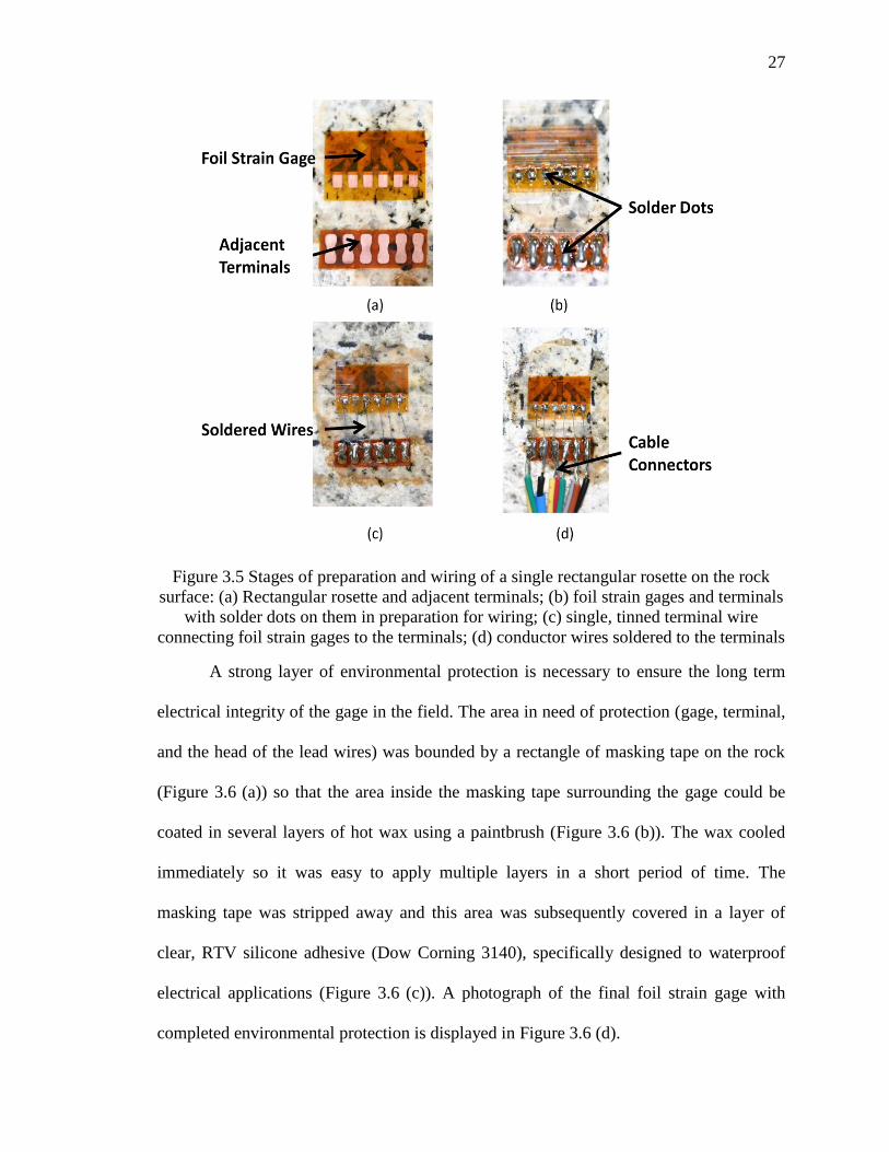
Figure 3.5 Stages of preparation and wiring of a single rectangular rosette on the rock
surface: (a) Rectangular rosette and adjacent terminals; (b) foil strain gages and terminals
with solder dots on them in preparation for wiring; (c) single, tinned terminal wire
connecting foil strain gages to the terminals; (d) conductor wires soldered to the terminals
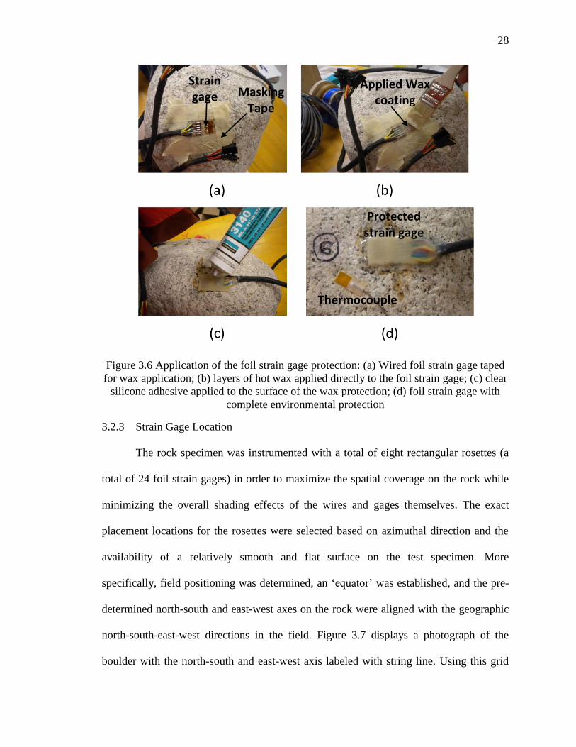
A strong layer of environmental protection is necessary to ensure the long term
electrical integrity of the gage in the field. The area in need of protection (gage, terminal,
and the head of the lead wires) was bounded by a rectangle of masking tape on the rock
(Figure 3.6 (a)) so that the area inside the masking tape surrounding the gage could be
coated in several layers of hot wax using a paintbrush (Figure 3.6 (b)). The wax cooled
immediately so it was easy to apply multiple layers in a short period of time. The
masking tape was stripped away and this area was subsequently covered in a layer of
clear, RTV silicone adhesive (Dow Corning 3140), specifically designed to waterproof
electrical applications (Figure 3.6 (c)). A photograph of the final foil strain gage with
completed environmental protection is displayed in Figure 3.6 (d).
28
Figure 3.6 Application of the foil strain gage protection: (a) Wired foil strain gage taped
for wax application; (b) layers of hot wax applied directly to the foil strain gage; (c) clear
silicone adhesive applied to the surface of the wax protection; (d) foil strain gage with
complete environmental protection
3.2.3 Strain Gage Location
The rock specimen was instrumented with a total of eight rectangular rosettes (a
total of 24 foil strain gages) in order to maximize the spatial coverage on the rock while
minimizing the overall shading effects of the wires and gages themselves. The exact
placement locations for the rosettes were selected based on azimuthal direction and the
availability of a relatively smooth and flat surface on the test specimen. More
specifically, field positioning was determined, an „equator‟ was established, and the pre-
determined north-south and east-west axes on the rock were aligned with the geographic
north-south-east-west directions in the field. Figure 3.7 displays a photograph of the
boulder with the north-south and east-west axis labeled with string line. Using this grid
Strain gage Masking
Tape
Applied Wax coating
Protected strain gage
Thermocouple

29
system, a gage was placed on the top and bottom of the rock, and on the equator,
positioned on the north, east, south and west sides of the rock. In addition to the top,
bottom, and four equator gages, two additional gages were positioned on the northeast
and the southwest quadrants of the rock between the equator and the top and bottom of
the specimen, respectively. Figure 3.7 displays the top strain gage near the intersection of
both major axis and the south and east equator gages on the boulder.
Figure 3.7. North–south and east-west axis established on the boulder with the top gage
and the south and east equator gages displayed
In general, the top and bottom gages were installed on surfaces that were
relatively horizontal, and the equator gages were installed on surfaces that were relatively
vertical when the boulder was in the field position. The additional NE gage was installed
on a surface that was upward facing and the SW gage was installed on a surface that was
downward facing. Overall, these locations were selected to document the spatial
variability in diurnal heating and strain given the constraints of having only eight
measurement locations. The orientation of each rosette was selected to ensure that cables
were efficiently oriented to minimize surface coverage (attached wires would lead down
S1 (Top)
S3 (East Equator )
S4 (South Equator )

30
instead of across the boulder). There was no attempt to place the strain gages on
particular minerals or in particular orientations. However, there was an attempt to
document their orientations relative to the grid system by horizontally projecting both
grid lines and measuring the orientation of gage 1 on the rosette with respect to them
using a protractor.
3.2.4 Summary on Strain Gage Measurement
It is important to note that because the boulder is rounded, there is potential error
in the principle strain calculations. The mathematics of foil strain gage calculations
assume the gage is attached to a flat, smooth surface that extends infinitely in all
directions. Therefore, it may be necessary to rely on the „relative‟ magnitude, sign, and
behavior of the strain gages rather than the absolute magnitude of the data when
evaluating the surface strain conditions. Since the strain gage configuration, calculations,
and programming remained unchanged from the previous study (Garbini, 2009),
additional validation and calibration was unnecessary.
3.3 Measurement of Surface Temperature
A thermocouple is constructed by creating a junction between two different types
of metal wires, which produces a voltage differential that is dependent upon temperature.
A standard T-Type thermocouple (Omega SA1XL-T-120) with a copper-constantan
junction was utilized for this project (Figure 3.8 (a)). This type of temperature
measurement sensor is a standard in a wide variety of engineering field studies that
require measurement of surface temperature on various materials due to the durability,
repeatability, and responsiveness of the sensor. It is capable of functioning in
temperatures ranging from -200 oC – 350
oC with a sensitivity of 43 µV/°C.

31
Figure 3.8 Thermocouple Installation: (a) cement adhesive used to attach all
thermocouples; (b) T-Type (copper-constantan) thermocouple; (c) T-Type thermocouple
installed on the surface of the boulder next to a protected strain rosette
A cement adhesive (Omegabond 400) was used to attach all thermocouples to the
rock test specimen. The adhesive was delivered in powder form, and mixed with water
until a paste consistency was achieved (Figure 3.8(b)). The adhesive backing on the
sensor was removed, and the cement adhesive was applied to the back of the
thermocouple in sufficient quantity to provide a complete contact with the rock upon
attachment. It was then attached to the rock and held under pressure until it cured
(approximately 5 - 7 minutes depending on ambient temperature).
Each thermocouple was positioned adjacent to a foil strain gage location (a total
of eight thermocouples) so that strain and temperature could accurately be assessed
relative to one another at all measurement locations. Figure 3.8(c) displays a photograph
of an installed thermocouple adjacent to a foil strain gage that has environmental
protection. While the thermocouples came pre-calibrated, all thermocouples were

32
validated against an independent thermometer to ensure the data acquisition system was
reading the sensors properly.
3.4 Measurement of Acoustic Emissions
Acoustic emissions are defined as transient elastic waves generated by the rapid
release of strain energy or by the sudden redistribution of stress within a material.
Sources of acoustic emission activity in rock can include defect-related deformation
(friction between interlocking grain boundaries), the initiation and propagation of
microcracks, and plastic deformation (Rao, 1998; Lei et al., 2000; Khair, 1981). The
purpose of an acoustic emission sensor (also referred to as a piezoelectric transducer) is
to convert the mechanical energy carried by an elastic wave into an electrical signal.
It is important to distinguish the difference between an AE “hit” and an AE
“event”. If the elastic wave measurement exceeds a pre-defined threshold value (already
established by Garbini (2009)) and is measured by one of the pre-amplified sensors
attached to the specimen, data will be recorded and referred to as an acoustic emission
“hit”. If the same wave is registered by at least four sensors on the specimen at the same
relative time, it is referred to as an acoustic emission “event”. The sophisticated source
code contained within this second software package (AE Win) requires an “event” to
calculate the three-dimensional source location of an AE wave.
Physical Acoustics Corporation equipment, sensors, and software were selected
because this was the only domestic vendor at the time that was able to provide software
that could locate an AE event in three dimensions. Figure 3.9 displays a photograph of
the AE sensor (PK151) utilized during this study. Inside the metal casing, the active
element of a piezoelectric transducer is a thin disk of piezoelectric material (a material
that can convert mechanical deformation into electrical voltage) coated in metal on the

33
top and bottom for electrical contact, and mounted in the metal cylinder case to provide
electromagnetic interference shielding. A damping material surrounds the piezoelectric
element to dissipate noise in the disk, and a wear plate is located under the piezoelectric
element to provide mechanical support to the disk. Six AE sensors were installed and a
SH-II data acquisition system monitored all AE activity. An adhesive couplant must be
used to attach the gage while ensuring that voids do not exist between the specimen and
sensor.
Figure 3.9 (a) Schematic of an acoustic emission sensor; (b) Physical Acoustics
Corporation acoustic emission sensor utilized during this study (PK151)
The SH-II data acquisition system utilizes two software programs to monitor and
analyze acoustic emissions. The “SH Client” software controls all primary
communications with the AE sensors on the rock during the calibration process and
during the data collection period. It is also used to set up all initial configurations for the
hardware. The field data collected by the “SH Client” software is then imported into the
“AE Win” software for data analysis.
The velocity of the AE wave is dependent upon the material properties and the
magnitude of this value is utilized in conjunction with the locations of the sensors to

34
determine the location of a micro-crack. As part of a detailed calibration process, it is
necessary to determine the wave velocity of the material and properly position the
sensors on the test specimen to enable the software to locate the source of the emission.
Each acoustic emission reaches a different AE transducer at a slightly different time
depending upon the distance between the source of AE (i.e. location of micro-crack) and
each AE sensor. The following subsections describe the sensor selection, and the
processes involved in determining the wave velocity and sensor locations.
3.4.1 Acoustic Emission Sensor Selection
The equipment and sensors must be sustainable in a natural, outdoor environment
since this is a field-based project. Based on trial and error, a low frequency (100 – 450
kHz), pre-amplified, low power consumption sensor was selected with the help the
manufacturer (Figure 3.9).
Two to six sensors are required depending upon the application (whether linear
location, zonal location, or point location measurements are needed). For the three
dimensional boulder in this study, point location (x, y, and z coordinates in a three
dimensional domain) is required. The software specifications require the inclusion of four
sensors to provide “point” location capability but the use of additional sensors is
recommended to better cover the surface of the specimen. The number and position of the
sensors can only be validated through trial and error.
3.4.2 AE Sensor Installation
Each AE sensor must be in full contact with the specimen (voids cannot exist
between the sensor and the test material), which presents a challenge on a boulder that
has a relatively rough surface and naturally occurring irregularities. To ensure the
adhesive would provide excellent contact between material and sensor and withstand the

35
environmental conditions in the field, a two part epoxy was used (E-20NS Loctitite Hysol
Epoxy). The strength of this epoxy increases if cured under heat, and the small ring of
adhesive around the installed sensor ensured that an adequate amount of adhesive was
utilized to enable full contact between the sensor and the test specimen. Figure 3.10
displays a photograph of the boulder in the field with the acoustic emission sensors
installed. Note that one sensor did fall off about 2 months after field deployment due to
the weight of the sensor in conjunction with the orientation of the surface plane it was
attached to (a relatively vertical face). While the sensor can be re-attached successfully in
the field, it is preferable to install the sensors on sub-vertical, upward facing faces of the
test specimen.
Figure 3.10 Acoustic emission sensors, foil strain gages, surface moisture sensor, and
thermocouples installed on the boulder
Surface Moisture
Sensor
Protected
Strain gages
Thermocouple AE Sensors

36
3.4.3 Finding Wave Velocity
As part of a detailed calibration process, it is necessary to determine the wave
velocity of the acoustic emission through the rock and properly position the sensors on
the test specimen to enable the software to locate the source of the emission. The “wave
velocity” is a material dependent property that can vary significantly in magnitude. For
example, the wave velocity in water is approximately 1,500 m/s and it can be as high as
5,500 m/s in rock. In this example, the difference in magnitude is attributed to the particle
to particle interaction. Water is a continuous medium while voids exist between the
particles in rock, which enable a wave to travel with less resistance.
In this study, the wave-velocity was determined using two rectangular blocks
specially cut from the same parent rock material so that simple, geometry (origin located
at one corner of the calibration block) could be used to determine distances between each
AE sensor installed on the calibration specimen. Each acoustic emission reaches a
different AE transducer at a slightly different time depending upon the distance between
the source of AE (i.e. location of micro-crack) and each AE sensor. This information is
utilized with the wave velocity to determine the three dimensional location. With the
sensors in position on the calibration block (the method used to position the sensors to
achieve optimum results is described in a subsequent paragraph), an AE event was
simulated using a „Pencil Lead Break‟ test (in accordance with the American Society for
Testing and Materials standard specification ASTM E 976) to determine this material
property.
To conduct a PLB test, a small piece of lead from a mechanical pencil
(approximately 2 to 3 mm in length) is snapped at a 28 angle from the surface at a
known location (see Figure 3.11 (b)). Knowing the true x, y, and z coordinates of each

37
sensor and the PLB location on the calibration block (easily determined using the
established origin of the rectangular block), multiple Pencil Lead Break (PLB) tests were
performed, and the AE data acquisition system was able to record the time it took each
sensor to register the PLB activity induced on the material so that the velocity of the
wave could be calculated using the time duration and distances between the source of the
wave and each sensor.
3.4.4 AE Sensor Location and Validation Test
The AEWin software configurations used by Garbini (2009) prevented the
software from distinguishing between interior versus exterior events. If an event occurred
on the interior of the rock, the software extrapolated the source location of the AE event
to the nearest surface on the specimen. This particular software configuration was
designed to monitor the structural health of tanks, pipes, and storage facilities, which are
hollow structures.
During this study, the ability to differentiate between interior and exterior events
was realized by changing the software settings and better positioning the sensors on the
test specimen. The manufacturer of AEWin suggested positioning the sensors so that “no
four sensors are on the same plane”. With six sensors, this could be accomplished by
creating two planes which are perpendicular to each other. Each plane was formed using
three sensors which were placed such that they try to form equilateral triangles. While
placing the sensors, no four sensors should form a plane. All combinations must be
checked to reach the optimum orientation. When an event occurs, the software algorithms
essentially develop an imaginary three-dimensional tetrahedron whose points comprise of
the sensors associated with the first four hits of the event, and then the software searches
for the AE source location within the tetrahedron developed using a best fit algorithm .

38
This method for finding the location is similar to various curve fitting algorithms.
However, if those four sensors are located on the same plane, the AE win software
algorithms are unable to create the three-dimensional tetrahedron required to determine
the source location, and hence there is a large error along the axis perpendicular to that
plane.
Using the above guidelines, sensor locations were selected on the calibration rock
to create multiple, triangular grid patterns between the sensors that created an optimized
pattern for the software to identify AE source location. Figure 3.11 (a) displays the
calibration block with the AE sensors temporarily attached. The dimensions of the first
calibration block were 137.6 mm in length (x-axis), 87.63 mm in width (y-axis), and
77.93 mm in height (z-axis). Figure 3.12 displays the calibration block and sensor
position configuration of the layout file in AE Win.
Figure 3.11 (a) Calibration block with acoustic emission sensors temporarily attached
with adhesive tape; (b) Pencil Lead Break Test performed on the calibration block in
accordance with ASTM E 976

39
Figure 3.12 Calibration block and AE sensors in AE Win software
Table 3.1 shows the 3D coordinate of sensors on the calibration block. Recalling
that any three AE sensors must form an equilateral triangle and form two perpendicular
planes, note that sensors 1, 2, and 3 form one triangle in the Y-Z plane and sensors 4, 5,
6 form another triangle in the X-Y plane. Additionally, sensors 1, 3, 6 form a slanting
plane. For example, if an event occurred near sensor 3, to calculate the location, AEWin
would create a tetrahedron using the first four hits. It could be sensors 3, 5, 6 and 1.
Hence it is important to note that no four sensors form a single plane.
Table 3.1 3D Coordinates of sensors on the calibration block
Using these sensor locations, wave velocity was determined using the PLB
procedure described in the last section. The average wave velocity was determined to be
Imaginary
Tetrahedron

40
5,353,501 mm/s. To validate this value, this value was inputted in the software, and used
to verify the location of all subsequent PLB tests. This validation exercise was performed
10 times in seven different PLB locations on the surface of the calibration rock. The
average source location calculated by “AEWin” was within 10.1 mm on average
(standard deviation equal to 2.4 mm) of the actual PLB location on the calibration block,
which was well within the tolerable limit of error for this study.
Subsequently, the same process was repeated for the second calibration block cut
from a separate boulder from the same parent rock material, resulting in an average wave
velocity equal to 2,293,201 mm/s. To validate this value on the second test specimen, it
was inputted in the software, and used to verify the location of all subsequent PLB tests.
This validation exercise was performed 10 times in six different locations, and the
average source location calculated by “AEWin” was within 11.3 mm on average
(standard deviation equal to 4.8 mm) of the actual PLB location on the calibration block.
Noting the difference in wave velocity values for two calibration blocks that were cut
from the same parent rock material, this initial calibration step was only one of several
iterations performed to determine the most accurate wave velocity value for the test
specimen, which was a required input value in “AEWin” to determine accurate locations.
After determining the wave velocity on a geometrically simple specimen, the
same validation exercise was repeated on the actual field specimen. Before validation
could proceed, the AE sensor locations were identified on the spherical boulder using the
same method already described: “no four sensors were on the same plane”. Since the
coordinates of a relatively spherical specimen were difficult to establish in comparison to
the simple geometry of a rectangular cube, a three sided corner box was constructed so
that the boulder could be placed inside of it and the x, y, and z coordinates could more

41
easily and accurately be determined (Figure 3.13). The origin of the coordinate system (0,
0, 0) was located at the intersection of these three sides.
Figure 3.13 Three sided box used to measure the x, y, and z coordinates on the boulder
Since the test specimen is not a cube, the software was configured using the “free
space” option using the determined wave velocity. In this configuration, the software
assumes that the sensors are placed in free space and AE waves travel with the wave
velocity mentioned in the layout file. Figure 3.14, Figure 3.15 and Figure 3.16 show the
side views of the test specimen with the AE sensors attached on them. The AE sensors
are numbered in the figures, as are the strain gages and thermocouples. Figure 3.17
displays the configuration of the AE sensors in a free space on the layout file in AEWin.
Table 3.2 shows the coordinates of the AE sensors on the sphere.
(0,0,0) y
z
x

42
Figure 3.14 AE Sensor (numbered) location: Side View of the test specimen ( North-
South )
Figure 3.15 AE Sensor (numbered) location: Side View of the test specimen (West-East)
North South
Bottom
Top
West East
Bottom
Top
1
2
6
5
6
2
3
1
Surface Moisture
Sensor
Thermocouples
Strain gages
South North
Thermocouple

43
Figure 3.16 AE Sensor (numbered) location: Side View of the test specimen (East-West)
Figure 3.17 AE sensors in free space in AE Win software
West East
Bottom
Top
1
5
4
Strain gage
Thermocouple

44
Table 3.2 3D coordinates of AE sensors on the test specimen
Using the newly established wave velocity from the second calibration block as
input in “AEWin”, PLB tests were performed at various locations on the boulder, and the
measured versus actual coordinates of each PLB test were compared. Initially, we got
acceptable readings at most of the PLB test locations with the exception of one area on
the boulder (near the location of the dimple displayed on Figure 3.2 (f)). Because that
portion of the rock was not well represented by an AE sensor, the AEWin software was
unable to accurately locate AE sources in this area (the coverage was incomplete within
this area of the rock which affected the ability for the software to calculate accurate
locations). As part of the iterative, trial and error process, one sensor was moved from the
bottom of the rock to the top of the dimple. The validation exercise was repeated and the
difference between the measured coordinates and actual coordinates of the PLB test was
reduced.
As a last step to further refine the 2,293,201 mm/s wave velocity, this value was
systematically varied in magnitude until the coordinates more closely converged. Values
of 2,200,000 mm/s, 2,400,000 mm/s, 2,600,000 mm/s, and 2,800,000 mm/s were
evaluated. The best results were achieved on the boulder using an average wave velocity
equal to 2,400,000 mm/s. This value was inputted into the software, the validation
exercise was performed 10 times in five different locations on the boulder, and the
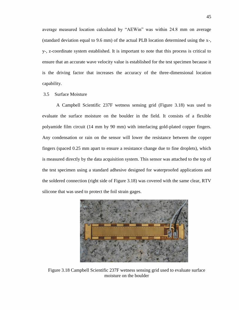
45
average measured location calculated by “AEWin” was within 24.8 mm on average
(standard deviation equal to 9.6 mm) of the actual PLB location determined using the x-,
y-, z-coordinate system established. It is important to note that this process is critical to
ensure that an accurate wave velocity value is established for the test specimen because it
is the driving factor that increases the accuracy of the three-dimensional location
capability.
3.5 Surface Moisture
A Campbell Scientific 237F wetness sensing grid (Figure 3.18) was used to
evaluate the surface moisture on the boulder in the field. It consists of a flexible
polyamide film circuit (14 mm by 90 mm) with interlacing gold-plated copper fingers.
Any condensation or rain on the sensor will lower the resistance between the copper
fingers (spaced 0.25 mm apart to ensure a resistance change due to fine droplets), which
is measured directly by the data acquisition system. This sensor was attached to the top of
the test specimen using a standard adhesive designed for waterproofed applications and
the soldered connection (right side of Figure 3.18) was covered with the same clear, RTV
silicone that was used to protect the foil strain gages.
Figure 3.18 Campbell Scientific 237F wetness sensing grid used to evaluate surface
moisture on the boulder

46
The level of resistance as a function of moisture was evaluated in a controlled
laboratory environment to calibrate the sensor. When there was moisture on the sensor,
the resistance measured by the sensor ranged between 2000 and 200,000 . When the
sensor was completely dry, the resistance was significantly higher reaching levels as high
as 7,000,000 . During this study, moisture was labeled “present” on the test specimen if
the resistance was less than or equal to 200,000 . Otherwise, the surface of the test
specimen was considered dry.
3.6 Measurement of the Environmental Conditions
In order to monitor the ambient environmental conditions surrounding the boulder
deployed to the North Carolina site, a full weather station capable of measuring ambient
temperature, relative humidity, wind speed, wind direction, barometric pressure,
insolation and precipitation was installed on site (components are labeled on Figure 3.19).
Since the Campbell Scientific and Physical Acoustics Corporation data acquisition
systems had already been purchased and tested as part of a previous study, it was
necessary to integrate the environmental sensors into the existing data acquisition
configuration rather than purchase an additional standalone system that would make data
integration difficult. Therefore, all environmental instrumentation was purchased from
Campbell Scientific to ensure the sensors would be compatible with the CR1000 logger.
A CS215 ambient temperature and relative humidity probe that outputs an SDI-12
signal directly to the data acquisition system was housed inside a naturally spirated, 6-
plate radiation shield (CS41303-5). When exposed to sunlight, the probe must be housed
inside a shield, which is white in color to reflect solar radiation, and enables air to pass
freely through the shield to keep the temperature probe at or near the ambient level.

47
Figure 3.19 (a) Campbell Scientific weather station installed at the field site; (b) ambient
temperature and relative humidity probe inside the radiation shield; (c) wind sentry set
for measurement of wind speed and direction; (d) pyranometer for measurement of
insolation; (e) barometric pressure sensor; (f) tipping bucket funnel for measurement of
precipitation
A CS03002 wind sentry set was utilized to measure wind speed and direction.
This system uses a three-cup anemometer to measure wind speed. Rotation of the cup
48
wheel produces a sine wave that is directly proportional to wind speed. The frequency of
the sine wave is measured by the data acquisition pulse count channel and converted to
engineering units. Wind direction is measured using a potentiometer. The data acquisition
system applies an excitation voltage to the potentiometer, which outputs an analog
voltage signal that is directly proportional to the azimuth angle of the wind direction.
The CS300 Apogee silicon pyranometer utilizes a silicon photovoltaic detector
mounted in a cosine-corrected head to provide solar radiation measurements (sun plus
sky radiation) for the spectral range of 300 to 1100 nm. The standard output is 0.2
mV/Wm-2
. The dome-shaped head prevents water from accumulating on the sensor head,
and the cable is shielded and cased to prevent internal condensation.
A CS106 barometric pressure sensor measures barometric pressure within a 500
to 1100 millibar range. It outputs a linear signal of 0 – 2.5 Volts DC that is measured
directly by the data acquisition system. The sensor is encased in a plastic, protective shell
fitted with an intake valve for pressure equilibration, and was located inside the data
acquisition enclosure in the field.
A TE525 tipping bucket rain gage (manufactured by Texas Electronics) funnels
precipitation into a bucket mechanism that tips when filled to a calibrated level. A
magnet attached to the tipping mechanism actuates a switch as the bucket tips, and the
switch closure is counted by the pulse-counting circuitry of the data acquisition system.
This model has a 24.4 cm orifice and measures precipitation in 0.1 mm increments. It is
necessary to periodically (about once per month) clean the tipping bucket funnel of dust
and bird droppings in order to ensure proper functioning.

49
3.7 Soil Moisture
Although the boulder was not embedded in the ground, it was assumed that soil
moisture affects ground surface temperature, and therefore, the bottom temperature of the
boulder. A CS616 water content reflectometer measures the volumetric water content of
soil using time-domain measurement methods that are sensitive to the dielectric
permittivity of any material. The moisture probe consists of two 30 cm long stainless
steel rods connected to a printed circuit board encapsulated in epoxy. Since water has a
dielectric permittivity significantly larger than soil constituents, the resulting oscillation
frequency is dependent upon the average water content of the soil surrounding the rods.
A shielded, 4-conductor cable is connected to the circuit board to supply power to the
probe and monitor the output. The cable connects to one of the single-ended analog
inputs on the CR1000 data logger, which converts the square-wave output to a volumetric
water content. In the field, the probe was pushed vertically into the subsurface near the
test specimen.
Figure 3.20 displays the instrumented boulder positioned in the field next to the
soil moisture probe. The steel rods are already inserted into the subsurface and the epoxy
covered circuit board is showing in this photograph. The calibration curve supplied by the
manufacturer was verified in a controlled laboratory environment. A suite of compacted
soil samples were prepared at varying moisture contents, and the probe was utilized to
measure the moisture content for each sample for comparison to the actual moisture
content as measured by standard procedures.

50
Figure 3.20 Instrumented boulder in the field
Soil Moisture Probe

CHAPTER 4: DATA ACQUISITION AND ANALYSIS METHODS
There were two data acquisition systems that simultaneously collected all data for
this research project. The SH-II data acquisition system continuously monitored all AE
activity while the CR1000 data acquisition system was programmed to collect all surface
strain, surface temperature, surface moisture, weather data, and soil moisture data at
intervals of 60 seconds. The following sections will describe each system in detail. Figure
4.1(a) displays a photograph of the three enclosures installed in the field. From left to
right on this figure, this figure displays the Campbell Scientific system (white enclosure),
the Physical Acoustics Corporation system (gray enclosure), and an additional steel
enclosure that housed the solar panel regulator and one of the three 12 V batteries that
supported the solar panels. The remaining two batteries were housed inside a plastic box
located behind the steel enclosure. The data acquisition equipment was powered by two
115 Watt Solar Panels (Figure 4.1(b)), regulated by a Morningstar PS
regulator/controller. Both systems were connected to a wireless modem that enabled
remote connectivity so that data could be downloaded from a location off-site.
Each data acquisition system had a separate data download procedure since each
data set was recorded in a different format. For analysis, the two data sets were merged
into a single Excel data analysis spreadsheet for each 24 hour time period that included
graphs for a visual display of the behaviors exhibited by the sensors. At the same time,

52
MATLAB programming was generated to analyze data in these spreadsheets in more
depth numerically and graphically. The following sections in this chapter describe the
data acquisition hardware, remote connectivity configuration, system power, and data
archival and analysis procedures in detail.
.
Figure 4.1 View of data acquisition enclosures, solar panel, test specimen, and weather
station (a) looking north; (b) looking west
Solar Panels
Campbell Scientific
SH-II and modem
Battery and Regulator
Weather Station

53
4.1 Data Acquisition
4.1.1 CR1000 Data Acquisition System
A Campbell Scientific CR1000 was utilized in this study (already configured in
the previous Garbini (2009) study). The Campbell Scientific CR1000 data logger can
drive and control external communication peripherals, is capable of data reduction, and
has 2 MB of flash memory for the operating system and 4 MB of battery-backed SRAM
for CPU usage, program storage, and data storage, which can be increased by using an
external Compact Flash card. The storage capacity for this system enabled the continuous
collection of data (without loss) over several days. The CR1000 has 16 single-ended or
eight differential analog input channels that will accommodate a wide variety of sensor
types including ratio-metric resistive bridge, thermocouple, switch closure, high
frequency pulse, low-level ac, and serial sensor input-output terminals. The CS I/O port
connects to an AC-powered PC and other communication peripherals (including phone
and multi-drop modems). A peripheral port enables data to be stored on a compact flash
card and also supports Ethernet communications. The RS-232 port provides a 9-pin DCE
port for connecting a battery powered laptop, serial sensors or RS-232 modems.
The data logger is powered using a 12 volt battery in conjunction with the CH100
charger/regulator and features a 13-bit analog to digital conversion rate, a 16-bit
microcontroller with 32-bit internal CPU architecture, and a battery-backed SRAM
memory and clock ensuring that all data, programs, and time stamps are maintained while
the CR1000 is disconnected from the main power source. Campbell Scientific data
acquisition systems are supported by LoggerNet software utilities, which provide setup
and network configurations, program management, programming (using a BASIC

54
programming language though the CRBasic Editor), communication, and data retrieval
and display capabilities.
Since the foil strain gages utilized during this study require the use of differential
channels, only eight foil strain gages could have been accommodated directly by the
CR1000 without multiplexing capabilities. To accommodate a total of 24 strain gages
(eight rectangular rosettes) and eight thermocouples, additional multiplexers were
connected to the CR1000 logger. Two Campbell Scientific AM16/32, 16-channel
multiplexers accommodated the 24 foil strain gages. However, terminal input modules
(serving as completion resistors) were attached directly to the multiplexer channels to
balance the last leg of the Wheatstone bridge circuit for all quarter bridge foil strain
gages. Additionally, a single AM 25T, 25-channel multiplexer accommodated the eight
thermocouples. The AM 25T houses a panel reference temperature (PRT) that is attached
to the multiplexer grounding bar to provide a reference temperature for the thermocouple
measurements. The sensors associated with the full weather station, a surface moisture
sensor, and a soil moisture sensor was connected directly to the CR1000 data logger.
Figure 3.1(a) displays the full hardware configuration of the data acquisition system
(before the cables were connected) including the CR1000 logger, two AM16/32
multiplexers, one AM25T multiplexer, and the CH100 charger/regulator, all of which
were housed inside a water-tight environmental enclosure.
4.1.2 Sensor Highway-II (SH-II) Data Acquisition System
The Physical Acoustics Corporation SH-II system was used to monitor all AE
activity during this study. The SH-II system (Figure 3.1(b)) is enclosed in a rugged
outdoor case, capable of operating in extreme weather conditions with minimum power
dissipations (temperatures ranging from -30 to 70oC without the use of heating or air

55
conditioning). The SH-II has a 4 GB internal flash card that stores the data until it is
extracted directly from the flash card or downloaded using a file transfer protocol via the
internet (the principle system interface). The system continuously monitors the data but
only records and saves data if hits (AE activity) are observed. To avoid data loss, data
should be downloaded often enough to avoid exceeding the capacity of the compact flash
card installed in the system, which is an issue on a rainy day.
The internal computer (CPU) is controlled by a Microsoft Windows CE 6.0
portable operating system. The SH-II contains surge protection, a circuit breaker for the
on/off switch, an AC/DC power supply, the main board, the CPU board, and two 4-
channel modules. The surge protector protects the system from unwanted power surges
on the input power line. The circuit breaker function disconnects the power from the
system in case of an excessive current draw. The main board is the digital back plane of
the system. From the DC input, the main board generates all necessary supply voltages
for the internal components. It also contains two, 4-million field-programmable gate
arrays (FPGA) that process the information from the 4-channel input boards and
communicate with the CPU board. The two, 4-channel modules (representing eight total
AE measurement channels) contain the analog circuitry for the system and process the
analog input signals from the sensors with the use of filters and analog/digital converters.
While six sensors are installed during this study, two additional channels are accessible
for future testing.
4.2 Remote Connectivity Communication
While it is possible to connect to both systems directly using a serial cable (for the
CR1000) or an Ethernet cable (for the SH-II), the intent was to enable remote
connectivity to accommodate daily download without traveling to the site. During this

56
study, both data acquisition systems were remotely accessed using a single, wireless
modem (Airlink Pinpoint X) housed inside the SH-II data acquisition enclosure. The
wireless modem connects to the internet using Code Division Multiple Access (CDMA)
technology via Verizon Wireless communications. The dynamic IP address (provided by
Verizon) is traceable using an IP manager software package provided with the modem.
This modem is compact, and has a fully‐featured mobile communications platform with
multiple peripheral connections including serial, Ethernet, and USB. Figure 4.2 shows
available connections on the modem. For this data acquisition configuration, the serial
port was used to connect the CR1000 and the Ethernet port was used to connect the SH-II
data acquisition systems.
Figure 4.2 Airlink Pinpoint X Connectors
Campbell Scientific Loggernet software is used to collect data from the CR1000.
For direct connection, Loggernet connects to CR1000 using the serial port on the
computer. For a remote connection, the CR1000 logger is connected to the modem using
the serial port on the modem (Figure 4.2), and the domain name and port number is
entered into Loggernet to establish the connection.
The SH-II data acquisition hardware creates an FTP server on the system. The
data from the SH-II can be downloaded using FTP client software (e.g. Filezilla) by

57
providing the IP address of SH-II, username and password. The Ethernet port is utilized
to establish a direct or a remote connection. For remote connectivity, the Ethernet port on
SH-II is connected to the wireless modem. Since SH-II acquires the IP address using
Dynamic Host Configuration Protocol (DHCP), connection can be accomplished using
the IP address of the modem (the domain name of the modem).
4.3 Power
Solar power was utilized to ensure continuous (uninterrupted) monitoring of the
rock specimen. Solar power supply was required to power the two data loggers and the
wireless modem. Table 4.1 shows the voltage and current characteristics of CR1000, SH-
II, and the modem.
Table 4.1 Voltage and Current Characteristic of Data Loggers and Modem
DC Voltage
(V)
Recommended
Voltage (V)
Current Drawn
(Amps) at 12 V
CR1000 9.6 to 16
12 0.11
SH-II 9 to 28 12 0.89
Pin Point X Airlink
Modem
9 to 28
12 0.3
The size of the solar panel is dependent upon the time of year that the study is
conducted and the location of the study. Because there is less sunlight during the winter
months, the required power was designed based on winter data to be conservative. During
the winter months in North Carolina, an average of four hours per day of sunlight is
assumed. There must be enough battery life to compensate for the remaining 20 hours per
day conservatively. The following calculations were performed to design the solar panel
and determine the number of batteries needed to back-up the panels.

58
Total Instantaneous Power = VCR1000 * ICR1000 + VSH-II * ISH-II + VModem * IModem [4.1]
= 15.6 Watts
Where : VCR1000 = 12 V
ICR1000 = 0.11 A
VSH-II = 12 V
ISH-II = 0.89 A
VModem = 12 V
IModem = 0.3 A
Total Instantaneous Current = Total Instantaneous Power / Voltage = 1.33 A [4.3]
Total Current in a day = Total Instantaneous Current * 24 = 31.92 Ah [4.4]
Considering 20% leakage and other transient currents,
Total Current required in a day = Total Current in a day * 1.20 = 38.30 Ah [4.5]
Hence a total current of 38.30 Ah is required by the two data loggers and the
modem. For the system to work even in winters, this much amount of current must be
drawn from the solar panel in 4 hours when there is sunlight and must be stored in
batteries.
Total Current required from solar panel in 4 hours = 38.30 [4.6]
Total Current required from solar panel in 1 hours = 38.30 / 4 = 9.57 A [4.7]
Considering 17 V solar panel,
Total power required = VoltageSolar Panel * Total Current required from a
Solar Panel in 1 hour = 162.69 Watts [4.8]
Where : VoltageSolar Panel = 17 V
Total Current required from Solar Panel in 1 hour = 9.57 A
For the given requirement of 17 V and 163 Watts, two 115 Watt Solar Panels
(Figure 4.1 (b)), and three 12V batteries were purchased. Table 4.2 shows the electrical

59
characteristic of the solar panel and Table 4.3 shows the specification of the batteries
used in this study.
Table 4.2 Electrical Characteristics of Solar Panel
Electrical Characteristics
Maximum Power ( Pmax ) 115 W
Voltage at Pmax (Vmp) 17.1 V
Current at Pmax (Imp) 6.7 A
Warranted minimum Pmax 109.3 W
Short-circuit current (Isc) 7.5 A
Open-circuit voltage (Voc) 21.8 V
Temperature coefficient of Isc 0.0650.015 %/ C
Temperature coefficient of Voc - 8010 mV/C
Temperature coefficient of power -0.50.05 %/ C
Table 4.3 Battery Specification
Nominal Voltage 12V
Capacity at C/100 110 AH
Plate Alloy Lead Calcium
Posts Forged terminals & bushings
Container/Cover: Polypropylene
Operating Temperature: - -40°C to 60°C
Cycle 2.40 to 2.43 VPC
Vent Self-sealing (2 PSI operation)
Terminal Dual Terminal S/X (SAE/STUD)
4.3.1 Battery Charge Controller
A pulse width modulator (PWM) Charge Controller regulates the power to limit
the rate at which electric current is added to or drawn from electric batteries. A
Morningstar PS regulator/controller is used which is located in the third steel enclosure

60
box displayed in Figure 4.1(a). Figure 4.3 shows the solar charge controller manufactured
by Morningstar, model number ProStar-15. Table 4.4 provides the electrical
specifications and battery control voltages of the regulator/controller, which prevents the
battery from overvoltage due to overcharging, and protects the battery against complete
discharge.
Table 4.4 Morningstar PS regulator/controller Specifications
Electrical Specifications
PS-15 Rated Solar Current 15A
Rated Load Current 15A
System Voltage 12V
Temp. Comp. (mV/˚C) 30mV
Min. voltage to operate 8V
Self-consumption 22mA
LVD current coefficient 20mV
Operating temperature 40˚C to + 60˚C
Operating temperature 30˚C to + 85˚C
Voltage accuracy 0.5%
Current accuracy 2.0%
Self-consumption 1 mA
Battery Voltage Set points
Battery Type Sealed
Regulation Voltage 14.15 V
Float 13.7 V
Equalization n/a 14.35 V
Load Disconnect 11.4 V
Load Reconnect 12.6 V
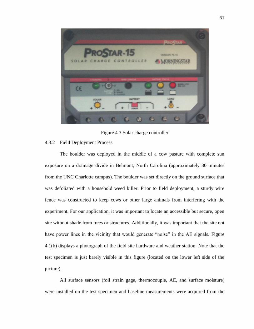
61
Figure 4.3 Solar charge controller
4.3.2 Field Deployment Process
The boulder was deployed in the middle of a cow pasture with complete sun
exposure on a drainage divide in Belmont, North Carolina (approximately 30 minutes
from the UNC Charlotte campus). The boulder was set directly on the ground surface that
was defoliated with a household weed killer. Prior to field deployment, a sturdy wire
fence was constructed to keep cows or other large animals from interfering with the
experiment. For our application, it was important to locate an accessible but secure, open
site without shade from trees or structures. Additionally, it was important that the site not
have power lines in the vicinity that would generate “noise” in the AE signals. Figure
4.1(b) displays a photograph of the field site hardware and weather station. Note that the
test specimen is just barely visible in this figure (located on the lower left side of the
picture).
All surface sensors (foil strain gage, thermocouple, AE, and surface moisture)
were installed on the test specimen and baseline measurements were acquired from the

62
strain gages in a controlled laboratory environment prior to field deployment. While the
cables for the AE sensors on the rock were easily screwed on to the sensors in the field
and the thermocouple wires were very thin and relatively easy to handle, the strain gage
cables were difficult to manage during the transit process due to the size, length (6.1 m),
and number (24) of cable bundles.
To avoid moving all 24 cable bundles after they had been soldered to the test
specimen and risk failing a gage during the transit and set-up process, an intermediate
“quick connection” was utilized. One side of the “quick connect” cable was soldered to
the eight intermediate terminal locations on the boulder (see Figure 4.4), the other side of
the quick connect cable was soldered to the 6.1 m long cable leads, the boulder was
carefully transferred to the field site, and the quick connection was completed on site.
However, this required additional splicing and the quick connection had to be water
proofed on site, (see Figure 4.5) which is generally not recommended if avoidable. It is
the author‟s opinion (after some trial and error) that potential problems associated with
the additional splicing and the water proofing techniques were significant and the benefits
of wiring and waterproofing a foil strain gage in a controlled atmosphere were more
important. As a result, the “quick connection” configuration will not be utilized on future
test specimens. To manage the cable bundles attached to the test specimen, it is
recommended that the rock be transported on a wooden pallet big enough to hold the
specimen and all cable bundles.
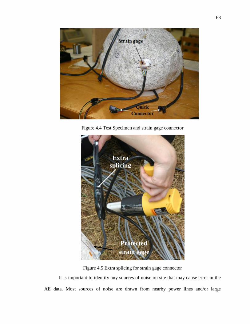
63
Figure 4.4 Test Specimen and strain gage connector
Figure 4.5 Extra splicing for strain gage connector
It is important to identify any sources of noise on site that may cause error in the
AE data. Most sources of noise are drawn from nearby power lines and/or large
Protected
strain gage
Extra
splicing

64
mechanical equipment. To determine potential sources of noise on site, raw data was
collected continuously for approximately one hour using the AE data acquisition system
and there were no hits or events during this time period at our chosen site. Previous rock
specimens installed on campus (on roof tops or closer to mechanical equipment near
buildings) and in off campus residential areas (closer to power line sources) clearly
showed noise issues in the data during an equivalent noise check exercise.
The field test specimen was oriented in the field in accordance with the north-
south-east-west axes pre-determined during the sensor installation process. The 3 m tall
tripod and steel mast for the weather station (Figure 3.19(a) and Figure 4.1(b)) was
constructed northwest of the rock to ensure minimum shading and all weather station
components were secured to it. The two data acquisition enclosures and an additional
steel box that housed the additional batteries and solar system regulator were set up north
of the rock on pallets resting on blocks to avoid moisture problems (Figure 4.1(a)).
Subsequently, all sensors were wired to the appropriate channels inside the data
acquisition boxes, all power components were wired to the loggers, and the two solar
panels were attached to the south-facing fence surrounding the test site (Figure 4.1(b)).
All cables and wires were wrapped with pipe insulation, which was covered with metal
duct tape to prevent rodents from chewing onto the wires (Figure 3.20), and all inlets on
the enclosure boxes were also sealed. A small, accessible shed was built around the three
enclosures (not shown in Figure 4.1(a)) to protect them from both heat and rain. Rodent
and ant traps were also put in place.
4.4 Data Archival Procedure
Because two data acquisition systems were required to monitor all sensors,
separate procedures were developed to download, archive, and manipulate each data set
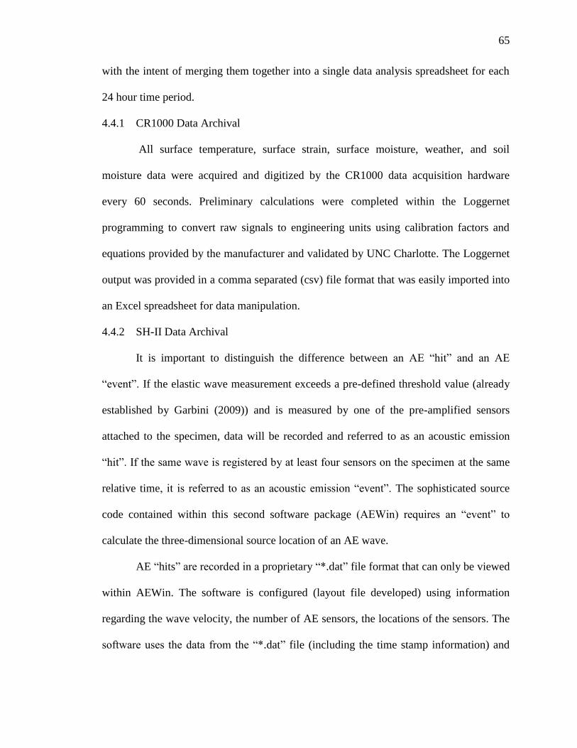
65
with the intent of merging them together into a single data analysis spreadsheet for each
24 hour time period.
4.4.1 CR1000 Data Archival
All surface temperature, surface strain, surface moisture, weather, and soil
moisture data were acquired and digitized by the CR1000 data acquisition hardware
every 60 seconds. Preliminary calculations were completed within the Loggernet
programming to convert raw signals to engineering units using calibration factors and
equations provided by the manufacturer and validated by UNC Charlotte. The Loggernet
output was provided in a comma separated (csv) file format that was easily imported into
an Excel spreadsheet for data manipulation.
4.4.2 SH-II Data Archival
It is important to distinguish the difference between an AE “hit” and an AE
“event”. If the elastic wave measurement exceeds a pre-defined threshold value (already
established by Garbini (2009)) and is measured by one of the pre-amplified sensors
attached to the specimen, data will be recorded and referred to as an acoustic emission
“hit”. If the same wave is registered by at least four sensors on the specimen at the same
relative time, it is referred to as an acoustic emission “event”. The sophisticated source
code contained within this second software package (AEWin) requires an “event” to
calculate the three-dimensional source location of an AE wave.
AE “hits” are recorded in a proprietary “*.dat” file format that can only be viewed
within AEWin. The software is configured (layout file developed) using information
regarding the wave velocity, the number of AE sensors, the locations of the sensors. The
software uses the data from the “*.dat” file (including the time stamp information) and
66
the software configurations within the layout file to determine the number of “events”
and the location of each “event”.
AEWin does not display data in a comma separated format that is easily imported
into Excel, and the SH-II system time stamp is recorded as cumulative time from the start
of data acquisition instead of using real time. Since the time stamp format is different for
each system (cumulative versus real time), it makes it more difficult to merge the data
sets together. To simplify this process, additional C programming was developed to read
the AE hit and event data, reconfigure it in a comma separated format, and convert the
cumulative time into an equivalent real time using the start time recorded at the beginning
of each data file.
More specifically, two separate C programs were developed (one for the “hits”
and one for the “events”). Since the CR1000 logger only recorded data every 60 seconds
and the SH-II system had the potential of recording data at a much higher frequency, the
number of hits and the number of events were summed up every 60 seconds so that the
two data sets could be easily merged together. The C program for the “hits” produced a
comma separated file that displayed the reconfigured time stamp, the number of hits per
channel each 60 seconds, and the total number of hits each 60 seconds. The C program
for the “events” produced a comma separated file that displayed the reconfigured time
stamp, and the number of events as well as the event location each 60 seconds.
4.4.3 Merging CR1000 and SH-II Dataset
The two datasets were downloaded every 1-2 days, but a separate spreadsheet was
created for each 24 hour interval (midnight to midnight) to merge all data together. To
simplify this process, an Excel spreadsheet was pre-programmed and pre-formatted as a
template file to perform all necessary calculations (e.g. calculate averages, look for

67
maximums, calculate rates) and create a suite of figures that accurately depicts the
behaviors of all measured data as a function of time for each 24 hour time period.
4.5 Data Analysis
Data was recorded every 60 seconds, every single day for a period of seven
months from June 20, 2010 to January 13, 2011. To handle this amount of data, two data
analysis methods were implemented. The Excel template file described in the previous
section generated the daily data and graphs necessary to visualize behaviors as a function
of time. Additionally, MATLAB programming was developed to reevaluate the same
spreadsheet data for the purpose of analyzing the data more globally. These methods are
described in more detail below.
4.5.1 Analysis using the Excel Spreadsheet Template
The Excel template file plots the following variables as a function of time after
the necessary calculations are performed within this template file: surface strain, surface
temperature, the range of surface temperatures for all thermocouples per minute, ambient
temperature, relative humidity, barometric pressure, insolation, wind speed, wind
direction, precipitation per minute, surface moisture per minute, soil moisture, minimum
and maximum principle strain, and principle strain orientation. Additionally, AE event
data is also displayed on the secondary axis of all graphs to help identify the conditions
that exist when AE events occur. It is important to note that AE data are collected
continuously so there may be multiple AE events in any particular minute.
An example of the figures generated by this spreadsheet method is displayed in
Figure 4.6 through Figure 4.9. In this figure all four graphs include a plot of the total
number of events occurring each minute throughout the day (right side axis). Figure 4.6
also displays the surface temperature from all 8 thermocouples and ambient temperature.

68
The approximate locations of thermocouples are as follows: 1-top; 1‟-northeast facing
upper hemisphere; 2-north facing equator; 3-east facing equator; 4-south facing equator;
5- west facing equator; 6- bottom; 6‟-southwest facing lower hemisphere.
Figure 4.7 also displays the temperature of the hottest thermocouple on the rock
minus that of the coolest for each minute of the day. Figure 4.8 also displays the wind
speed per minute and Figure 4.9 displays the maximum principle strain at each of the
eight strain measurement locations, which correspond closely with the thermocouple
locations.
Figure 4.6 Surface temperature versus Time

69
Figure 4.7 Maximum surface temperature difference across the rock versus time
Figure 4.8 Wind speed versus time
AE Events
AE Events
(symbols)
Temperature Difference

70
Figure 4.9 Maximum principle strain versus time
4.5.2 Analysis using MATLAB
For a more advanced numerical and graphical analysis of this large dataset,
MATLAB programs were written to read, manipulate, and summarize the data trends and
observations. For each event, the data is organized by time stamp, event location, and the
corresponding test specimen and weather data. A database was designed to facilitate a
detailed analysis of all AE events in conjunction with the corresponding test specimen
and environmental conditions so that behavioral patterns could be identified spatially and
temporally within and on the test specimen. During the analysis process, the program was
continuously updated to obtain a database that could generate summary statistics and
histograms of the variable and data of interest.
The program calculates the number of events per day, and the timestamp
(individual unique minute) associated with each acoustic emission event. To better
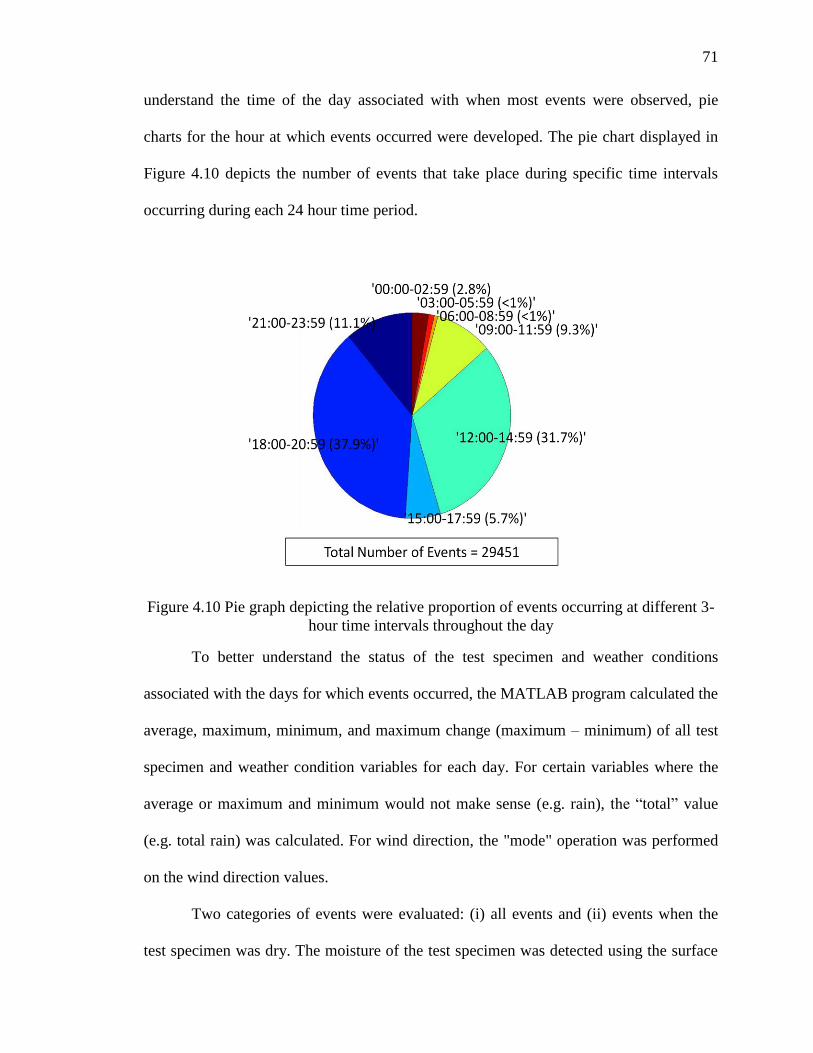
71
understand the time of the day associated with when most events were observed, pie
charts for the hour at which events occurred were developed. The pie chart displayed in
Figure 4.10 depicts the number of events that take place during specific time intervals
occurring during each 24 hour time period.
Figure 4.10 Pie graph depicting the relative proportion of events occurring at different 3-
hour time intervals throughout the day
To better understand the status of the test specimen and weather conditions
associated with the days for which events occurred, the MATLAB program calculated the
average, maximum, minimum, and maximum change (maximum – minimum) of all test
specimen and weather condition variables for each day. For certain variables where the
average or maximum and minimum would not make sense (e.g. rain), the “total” value
(e.g. total rain) was calculated. For wind direction, the "mode" operation was performed
on the wind direction values.
Two categories of events were evaluated: (i) all events and (ii) events when the
test specimen was dry. The moisture of the test specimen was detected using the surface

72
moisture. The test specimen was considered dry if the surface moisture sensor indicated
no moisture on it. The values generated in MATLAB were categorized in three separate
categories: (i) all day, (ii) days on which there was at least one event and (iii) days on
which there was at least one dry event.
To understand the instantaneous condition of the test specimen and weather
conditions when events occurred, all the strain, surface temperature, surface moisture and
weather data at the time when an event occurred was accumulated.
It was also desirable to evaluate the changes and condition of the test specimen
immediately before an event. The difference in all test specimen values (strain and
temperature) and weather condition variables was evaluated 1 minute, 5 minutes, 15
minutes, and 60 minutes prior to each event. In addition to this, the difference in the rate
of change of above values was also calculated. In some cases, the total values, and/or the
mean or mode was calculated instead (e.g. total rain in the last 15 minutes was
calculated). Histograms of all above calculated values were plotted along with the mean
and standard deviation.
Figure 4.11 shows histograms for relative humidity from June 20, 2010 to January
13, 2011. Figure 4.11(a) shows histogram of maximum recorded humidity recorded
every day. Similarly Figure 4.11(b) and (c) show histograms for minimum and average
relative humidity recorded every day. For Figure 4.11(d), first difference between the
maximum relative humidity and minimum relative humidity for each day is obtained and
then histogram of these values is plot in the figure. Mean and standard deviation is
displayed at top-right in all the figures.

73
Figure 4.11 (a) Maximum relative humidity; (b) minimum relative humidity; (c) average
relative humidity; (d) (maximum-minimum) relative humidity from June 20, 2010 to
January 13, 2010
In addition to analyzing the temporal patterns of AE events and boulder
conditions, AE event location patterns were examined. AEWin analyzes the AE hit data
to mathematically determine the three-dimensional location of all AE events (similar to
using multiple seismographs to determine the focus of an earthquake). In order to
visualize the locations and begin to identify spatial patterns, a three-dimensional shell of
the test specimen was generated within MATLAB using the dimensions of the test
specimen (length, width, and height) assuming an ellipsoid function.
As an example, Figure 4.12 displays two sample profile views of the test
specimen including four months of data from June 20, 2010 to September 25, 2010. In

74
this figure we only display events whose locations fall within our three-dimensional
ellipsoid. However a large number of event locations fell outside of this shell.
Approximately 11,250 events fell within the 5 cm error above the ellipsoid, leaving a
relatively large number of events outside of the ellipsoid. Events outside the ellipsoid are
interpreted to be due to reverberation of AE waves in the test specimen (i.e. secondary
waves associated with a prior event). If the amplitude of the reverberated wave is greater
than the threshold, it will also be detected as a hit. Such a wave would have traveled
almost twice the distance of the original wave, hence causing the calculated location of
the event to fall far afield of the boulder itself. Consequently, in this location analysis,
only events that fall inside the ellipsoid are considered.
Figure 4.12 Locations of AE events on the test specimen boulder: (a) profile view normal
looking east; (b) profile view looking north
4.5.3 Data Analysis Summary
The goal is to evaluate all the graphs generated by the Excel spreadsheets and the
MATLAB histograms to evaluate patterns in the data. Since every Excel graph displays
events on the secondary axis, the spatial and temporal patterns on the test specimen are
evaluated in combination with the ambient weather conditions during each event to help
identify patterns and behaviors before, during, and after an event.

75
When certain patterns were observed, MATLAB programs were developed to
generate numerical statistics to understand those patterns in more detail. For example,
when an event occurred, it was determined that the test specimen generally had a sudden
drop in temperature. To develop more insight into this pattern, the change of temperature
of test specimen in the previous 1, 5, 15 and 60 minutes for all instances when event
occurred was calculated. Similarly, combinations of graphs within the Excel spreadsheet
and the graphs and calculations produced from MATLAB were utilized to observe and
analyze.
The test specimen and weather conditions were monitored from June 20, 2010 to
January 13, 2011. Test specimen and weather conditions showed different patterns in
different seasons so the data analysis was divided into three seasons. In accordance with
the local meteorologist (John Wendal), the summer data extended from June 20, 2010 to
September 25, 2010, the fall data extended from September 26, 2010 to December 2,
2010, and the winter data extended from December 3, 2010 to January 13, 2011. An in
depth discussion of the data analysis is provided in the following chapter.

CHAPTER 5: RESULTS AND DISCUSSION
The purpose of this study is to correlate the formation of cracks in rock (as
measured by acoustic emission sensors) with the surface conditions of the boulder and
the ambient weather conditions that exist as a result of diurnal temperature variations
each day. Data was collected for a period of seven months from June 20, 2010 to January
13, 2011. The first part of this chapter discusses the daily and seasonal conditions of the
test specimen throughout the observation period as measured by the attached sensors
including general variations in surface temperature and corresponding strain. The
extreme temperature conditions that the rock underwent, the general temperature patterns
that were observed, and the general patterns of the surface strain due to temperature
variations were discussed. The second part of the chapter discusses the conditions of the
rock and surrounding environment in conjunction with the timing, location, duration, and
magnitude of AE events, which are assumed to signify the formation and/or propagation
of cracks. In total, 29,451 events were observed during a period of 194 days. The last
section of the chapter includes an interpretation of the results and observations.
Since this large dataset includes data from six AE sensors that are monitored
continuously and eight thermocouples, 24 strain gages, and a variety of weather station
sensors measured every minute for a period of 7 months, only the most significant
observations are shown in this chapter. Tables were generated to discuss the extreme
conditions and the general trends observed. The values in those tables were obtained
using MATLAB. Each table is preceded by an explanation on how the calculations are

77
performed and how it relates to the process contributing to the formation of the cracks. In
addition to tables, graphs were generated to reflect the observations made. Seasonal
variations were discussed.
Discussion of AE events are separated into two categories during the discussion: 1)
comparison of all events and 2) comparison of dry events. Dry events help to understand
the physical weathering processes that occur in the absence of moisture as measured by
the moisture sensor attached to the surface of the rock. As a result, separate tables and
graphs are generated for dry events in parts of the discussion. There are times when the
patterns for both categories are similar, and in these cases, common tables and figures
were generated.
5.1 Test specimen conditions throughout the observation period
5.1.1 General trends in surface temperature and strain
This section discusses the general trends observed by the sensors measuring
surface temperature and strain during this study to show that reasonable values were
measured. Figure 5.1 displays the ambient temperature as well as the temperature of all
eight thermocouples for a 24 hour time period on July 21, 2010. The secondary axis
displays the number of AE events observed on that day. AE events are indicated by the
symbols on this figure. This figure is representative of the trends that are typical of any
day during the study.
Figure 5.1 shows that surface temperatures are directly proportional to the
ambient temperatures that the test specimen was subjected to. For example, as the
ambient temperature increases from 24.07C to 34.33C between 6 AM and 3 PM, the
surface temperatures proportionally increase from 23.10C to 45.88C. Note that all
temperatures rise in the late morning and fall in the early evening, indicating that the
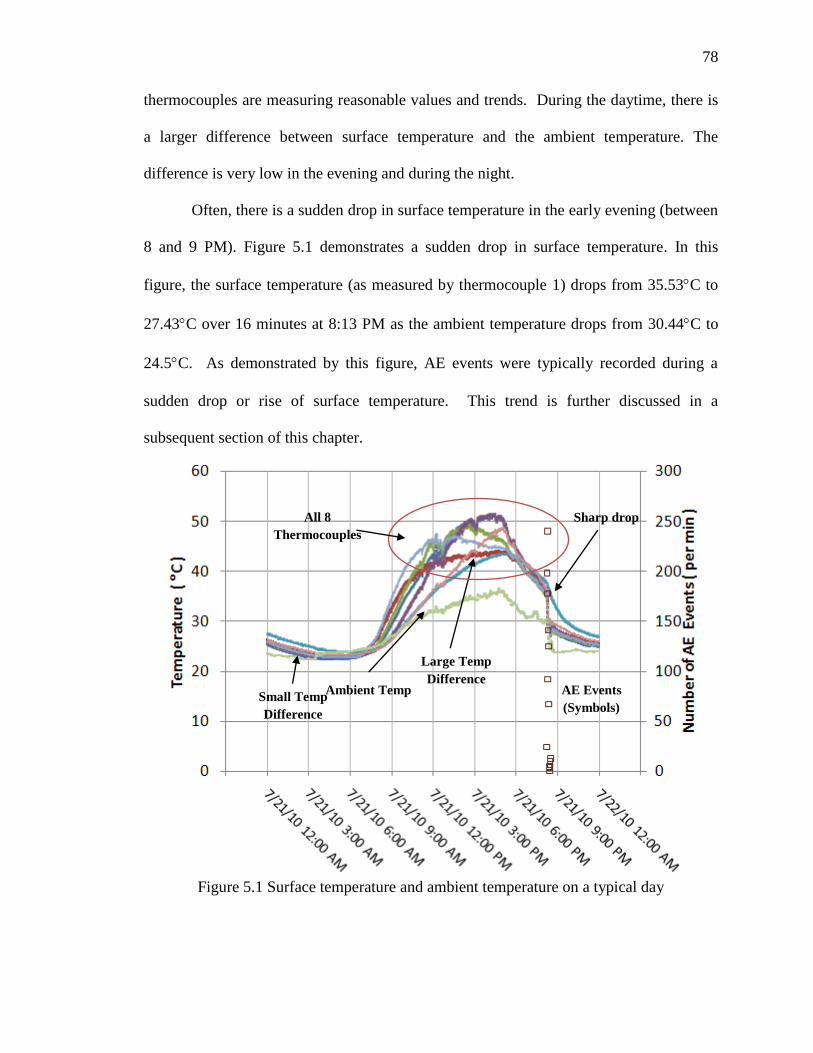
78
thermocouples are measuring reasonable values and trends. During the daytime, there is
a larger difference between surface temperature and the ambient temperature. The
difference is very low in the evening and during the night.
Often, there is a sudden drop in surface temperature in the early evening (between
8 and 9 PM). Figure 5.1 demonstrates a sudden drop in surface temperature. In this
figure, the surface temperature (as measured by thermocouple 1) drops from 35.53C to
27.43C over 16 minutes at 8:13 PM as the ambient temperature drops from 30.44C to
24.5C. As demonstrated by this figure, AE events were typically recorded during a
sudden drop or rise of surface temperature. This trend is further discussed in a
subsequent section of this chapter.
Figure 5.1 Surface temperature and ambient temperature on a typical day
Sharp drop
Large Temp
Difference AE Events
(Symbols)
Ambient Temp
All 8
Thermocouples
Small Temp
Difference

79
Figure 5.2 displays the strain measured by each of the individual gages on the
rectangular rosette for strain gage 1. Note that these raw strain readings are utilized to
calculate the major and minor principle strain values at each location in subsequent
discussions. Similar to surface temperature, strain is directly proportional to the ambient
temperature. When there is a rise in ambient temperature, there is increase in strain
(indicating expansion) and when there is drop in ambient temperature there is decrease in
stain (indicating compression). The surface temperature is also proportional to the
ambient temperature.
Figure 5.2 Strain measure on the three grids of a rectangular rosette on a typical day
Figure 5.3 illustrates the ambient temperature and the maximum principle strain
measured by the eight strain gages (S1, S2, S3, S4, S5, S6, S1‟, and S6‟) on July 21,
2010. These data are representative of all strain data collected during the testing interval.
Strain is plotted on the primary axis and ambient temperature is plotted on the secondary
axis. A positive strain value denotes tension (expansion) and a negative strain value
Thermocouple 1
S1, Grid 1
S1, Grid 2
S1, Grid 3
Ambient Temp

80
represents compression on the surface. It can be seen that the test specimen experiences
the greatest magnitude of strain when the maximum ambient temperature is attained
during that day.
Figure 5.3 Maximum principle strain on all 8 strain gages on a typical day
5.1.2 Temperature differences across the test specimen
Similar to Garbini (2009), various aspects (north-facing, south-facing, etc.) of the
rock measured different surface temperatures at different times of the day, causing a
temperature difference between different locations on the boulder. Table 5.1 lists the days
when the maximum temperature difference between two different locations on the test
specimen was the highest when evaluating all days within each of the three seasons
evaluated. To obtain the final data within this table, the temperature differences between
different locations on the rock were evaluated each minute, the largest difference
calculated from this analysis was then selected each minute, and then the maximum
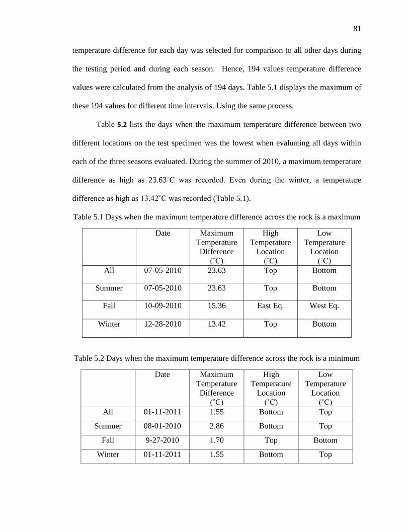
81
temperature difference for each day was selected for comparison to all other days during
the testing period and during each season. Hence, 194 values temperature difference
values were calculated from the analysis of 194 days. Table 5.1 displays the maximum of
these 194 values for different time intervals. Using the same process,
Table 5.2 lists the days when the maximum temperature difference between two
different locations on the test specimen was the lowest when evaluating all days within
each of the three seasons evaluated. During the summer of 2010, a maximum temperature
difference as high as 23.63˚C was recorded. Even during the winter, a temperature
difference as high as 13.42˚C was recorded (Table 5.1).
Table 5.1 Days when the maximum temperature difference across the rock is a maximum
Date Maximum
Temperature
Difference
(˚C)
High
Temperature
Location
(˚C)
Low
Temperature
Location
(˚C)
All 07-05-2010 23.63 Top Bottom
Summer 07-05-2010 23.63 Top Bottom
Fall 10-09-2010 15.36 East Eq. West Eq.
Winter 12-28-2010 13.42 Top Bottom
Table 5.2 Days when the maximum temperature difference across the rock is a minimum
Date Maximum
Temperature
Difference
(˚C)
High
Temperature
Location
(˚C)
Low
Temperature
Location
(˚C)
All 01-11-2011 1.55 Bottom Top
Summer 08-01-2010 2.86 Bottom Top
Fall 9-27-2010 1.70 Top Bottom
Winter 01-11-2011 1.55 Bottom Top

82
The reason for this temperature difference is the path of sun transit over the rock.
Figure 5.4 displays the surface temperature of all thermocouples on October 9, 2010.
This figure shows that the peak temperature is reached at different times of the day. For
example, the surface temperature located on the top of the rock (T1) reaches the peak
temperature around 4 PM while the surface temperature on the east side of the equator
(T3) reaches the peak temperature around 1 PM and the surface temperature on the south
side of the equator (T4) reaches the peak temperature around 5 PM.
Figure 5.4 Temperature peaks at different times of the day on October 9, 2010
For every minute, the difference between the thermocouple measuring the
maximum surface temperature and the thermocouple measuring the minimum surface
temperature is calculated and these data are presented on Figure 5.5 for a typical 24 hour
time period on October 9, 2010. The highest temperature differences exist between 10
T4 Peak T1 Peak
T3 Peak

83
AM and 6 PM. A maximum difference of 15.35˚C was observed on this date at 11:05
AM.
Figure 5.5 Difference in surface temperature (maximum – minimum) on the rock on
October 9, 2010
Figure 5.4 and Figure 5.5 displays data from the days when the maximum
temperature difference between different locations on the rock for a given day is the
highest in the fall season. Figure 5.6 and Figure 5.7 shows the trends observed when the
maximum temperature difference between different locations on the rock for a given day
is the lowest in the fall season. Figure 5.6 displays surface temperature data on September
27, 2010 for all thermocouples. The differences between these curves in the morning,
afternoon, and evening hours are minimal. Similarly, Figure 5.7 displays the maximum
difference in the surface temperature across on the rock on September 27, 2010. The
maximum temperature difference was only 1.69˚C during this fall season. Even in the

84
peek afternoon hours, it was approximately 1˚C. It is important to note that there was rain
throughout the day so there was no insolation measured from the sun and therefore, the
rock maintained a uniform temperature throughout the day.
Figure 5.6 Surface temperatures on the rock on September 27, 2010
Figure 5.7 Difference in surface temperature (maximum – minimum) of the rock on
September 27, 2010

85
Table 5.3 shows the surface temperature of the test specimen every three hours for
a 24 hour time period on July 5, 2010. This date was selected because the maximum
temperature difference across different locations on the rock was highest on this day. The
surface temperature is highest on the bottom of the rock during the night and early
morning time (see the 00:00, 3:00, 6:00 and 21:00 time periods in Table 5.3). During the
9:00, 12:00 and 15:00 time periods in Table 5.3, the surface temperatures on the top of
the rock are the highest. In the evening at 6 PM, the western side of the test specimen
measured the highest temperature while the eastern side measured the lowest
temperature.
Table 5.3 Surface temperature (˚C) on July 5, 2010
00:00 3:00 6:00 9:00 12:00 15:00 18:00 21:00 23:59
Top 19.2 17.7 16.2 34.4 49.8 56.7 47.6 23.26 20.2
North
Equator 23.4 18.9 16.1 26 37.4 42.7 43 33.28 24.66
East
Equator 22.4 18.4 15.6 31.4 44.6 42.6 38.5 30.5 23.9
South
Equator 22.6 18.4 15.6 24 40.9 45.9 41.3 31.9 24.1
West
Equator 23.1 18.7 15.8 21.6 34.3 45.9 49.4 33.5 24.3
Bottom 26 21.3 18.4 22.7 34.1 39.7 40.7 35.76 27.3
NE
High 22.9 18.5 15.6 30.7 42.2 43.1 40.2 31.97 24.12
SW
Low 24 19.5 16.7 21.4 34.4 43.6 45.9 33.99 25.28
Max
Temperature
26
(Bottom)
21.4
(Bottom)
18.4
(Bottom)
34.5
(Top)
49.8
(Top)
56.7
(Top)
49.4
(West)
35.7
(Bottom)
27.3
(Bottom)
Min
Temperature
19.2
(Top)
17.7
(Top)
15.6
(NE High)
21.5
(SW Low)
34
(SW Low)
39.7
(Bottom)
38.5
(East)
23.2
(Top)
20.2
(Bottom)
These trends are observed during all seven months of the study. These
temperature differences can cause expansion and contraction in the rock and induce
stresses within the rock over the course of the day. Daily repetition of these trends could

86
induce cyclic stresses on the rock and lead to formation of cracks by way of physical
weathering.
5.1.3 Rate of change of surface temperature
The value of each thermocouple reading was subtracted from the reading for the
previous minute to calculate the differences in surface temperature over each 60 second
interval during the day for all eight thermocouples. (This calculation is referred to as the
„rate of change of temperature‟ throughout the text in order to be consistent with cited
literature. It is not meant to imply acceleration). The thermocouple that had the
maximum rate of change for each minute was selected, and these data were utilized to
determine the maximum rate of surface temperature change for each day. Table 5.4
displays the highest and lowest maximum rate of change in the surface temperature
(maximum change in surface temperature per minute at a single location) per season and
for the entire testing period. Note that some areas of the test specimen experienced large
changes in surface temperature while other parts of the test specimen experienced
negligible change.
Table 5.4 Rate of change in surface temperature
Highest maximum rate of change Lowest maximum rate of change
Date Maximum
rate of
change in
temperature
(˚C/min)
Boulder
Location
Date Maximum
rate of
change in
Temperature
(˚C/min)
Boulder
Location
All 07-03-2010 15.89 Top 01-11-2011 0.26 Bottom
Summer 07-03-2010 15.89 Top 08-01-2010 0.44 Top
Fall 11-05-2010 4.10 East 9-29-2010 0.39 Bottom
Winter 01-13-2011 4.89 South 01-11-2011 0.26 Bottom
The table indicates that on certain days, a very high rate of change of surface
temperature was observed unlike other days when the maximum rate of change of surface
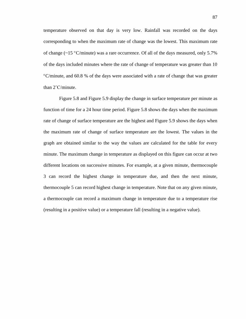
87
temperature observed on that day is very low. Rainfall was recorded on the days
corresponding to when the maximum rate of change was the lowest. This maximum rate
of change (~15 C/minute) was a rare occurrence. Of all of the days measured, only 5.7%
of the days included minutes where the rate of change of temperature was greater than 10
C/minute, and 60.8 % of the days were associated with a rate of change that was greater
than 2˚C/minute.
Figure 5.8 and Figure 5.9 display the change in surface temperature per minute as
function of time for a 24 hour time period. Figure 5.8 shows the days when the maximum
rate of change of surface temperature are the highest and Figure 5.9 shows the days when
the maximum rate of change of surface temperature are the lowest. The values in the
graph are obtained similar to the way the values are calculated for the table for every
minute. The maximum change in temperature as displayed on this figure can occur at two
different locations on successive minutes. For example, at a given minute, thermocouple
3 can record the highest change in temperature due, and then the next minute,
thermocouple 5 can record highest change in temperature. Note that on any given minute,
a thermocouple can record a maximum change in temperature due to a temperature rise
(resulting in a positive value) or a temperature fall (resulting in a negative value).

88
Figure 5.8 Rate of change of surface temperature on July 3, 2010
While all values displayed in Figure 5.9 are less than 2 °C/minute (an important
parameter noted in the literature by Hall( 1999) and Hall and Andre(2001)), Figure 5.8
displays a rate of change of surface temperature greater than 2 °C/minute 204 times on
August 1, 2010. However, AE events do not necessarily happen during each of these
instances. A rate of change in temperature greater than or equal to 2 °C/min does not
necessary cause cracks in rocks as suggested by Hall( 1999) and Hall and Andre(2001).
The purpose of this study is to determine the surface and ambient conditions that will
cause an AE event to take place. This subject is discussed in more detail in a subsequent
section of this chapter. These figures are representative of a typical day during the testing
period. Temperature changes can cause expansion and contraction in the rock due, which
can induce cyclic stresses on the rock and the possibility of crack formations (physical
weathering of the rock).
> 2 °C/minute
> 2 °C/minute

89
Figure 5.9 Rate of change of surface temperature on August 1, 2010
5.1.4 Strain exerted on the rock
Figure 5.10 and Figure 5.11 display examples of the general trends in surface
strain observed on the test specimen during this study. Please note that adjustments for
temperature compensation have not been incorporated into the strain calculations
presented in this document. Figure 5.10 (a), (b), and (c) displays the maximum and
minimum principle strain for gage 2 (located on the equator – north side) as a function of
time during a 24 hour time period in the summer, fall, and winter, respectively. Similarly,
Figure 5.11 (a), (b) and (c) displays the maximum and minimum principle strain values
recorded by gage 6 (located on the bottom of the rock) as a function of time during a 24
hour time period on the same representative days (typical representations of each season).
In other words, Figure 5.10(a) and Figure 5.11(a) both display strain for the same 24 hour
time period, but the strain conditions are representative of different locations (gage 2
versus gage 6). Surface temperature and ambient temperature is displayed on the
secondary axis of each figure.

90
Figure 5.10 Typical maximum and minimum principle strain values for gage S2 (located
on the equator, north side) during the (a) summer, (b) fall, and (c) winter
(a)
(b)
(c)
Sudden drop in surface
temperature and strain
Thermocouple, T2
Ambient Temperature
Max Principle Strain, S2
Min Principle Strain, S2
Thermocouple, T2
Ambient Temperature
Max Principle Strain, S2
Min Principle Strain, S2
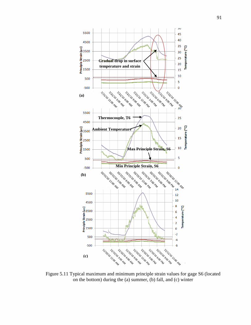
91
Figure 5.11 Typical maximum and minimum principle strain values for gage S6 (located
on the bottom) during the (a) summer, (b) fall, and (c) winter
(b)
(a)
(c)
Gradual drop in surface
temperature and strain
Thermocouple, T6
Ambient Temperature
Min Principle Strain, S6
Max Principle Strain, S6
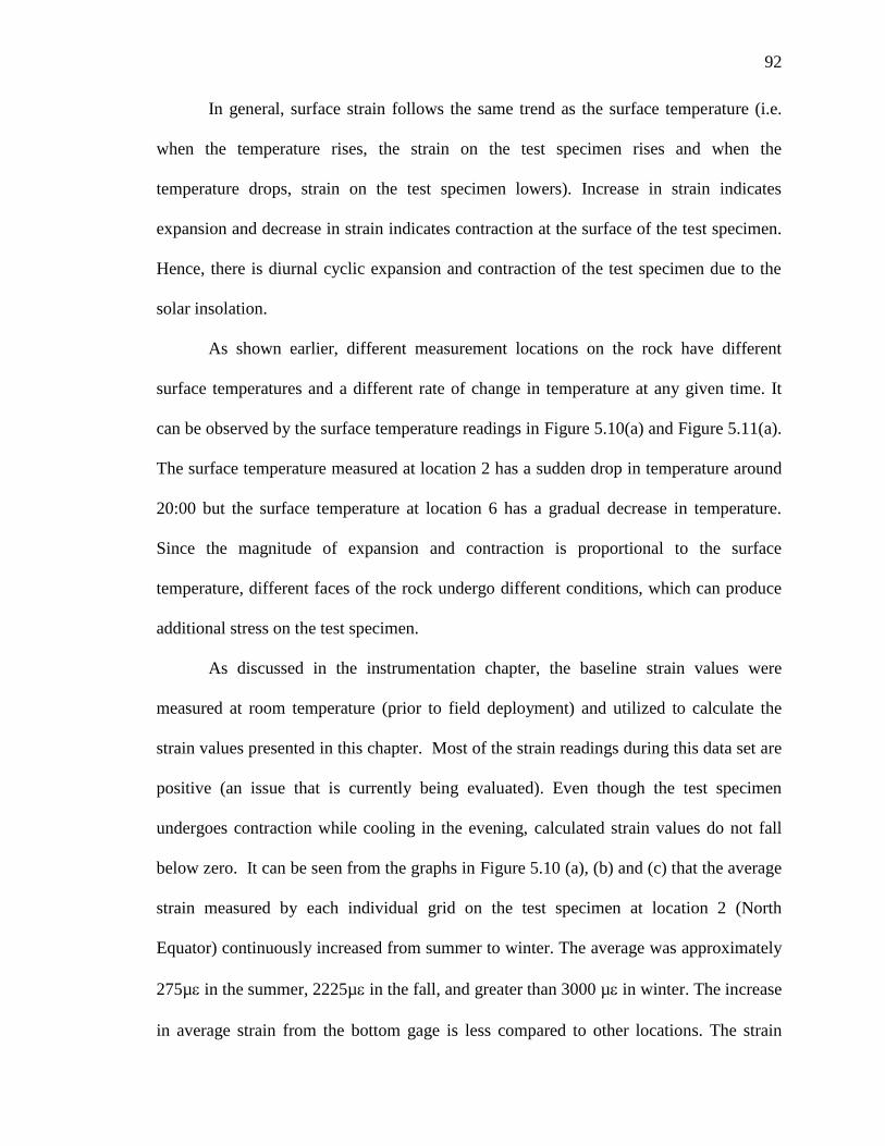
92
In general, surface strain follows the same trend as the surface temperature (i.e.
when the temperature rises, the strain on the test specimen rises and when the
temperature drops, strain on the test specimen lowers). Increase in strain indicates
expansion and decrease in strain indicates contraction at the surface of the test specimen.
Hence, there is diurnal cyclic expansion and contraction of the test specimen due to the
solar insolation.
As shown earlier, different measurement locations on the rock have different
surface temperatures and a different rate of change in temperature at any given time. It
can be observed by the surface temperature readings in Figure 5.10(a) and Figure 5.11(a).
The surface temperature measured at location 2 has a sudden drop in temperature around
20:00 but the surface temperature at location 6 has a gradual decrease in temperature.
Since the magnitude of expansion and contraction is proportional to the surface
temperature, different faces of the rock undergo different conditions, which can produce
additional stress on the test specimen.
As discussed in the instrumentation chapter, the baseline strain values were
measured at room temperature (prior to field deployment) and utilized to calculate the
strain values presented in this chapter. Most of the strain readings during this data set are
positive (an issue that is currently being evaluated). Even though the test specimen
undergoes contraction while cooling in the evening, calculated strain values do not fall
below zero. It can be seen from the graphs in Figure 5.10 (a), (b) and (c) that the average
strain measured by each individual grid on the test specimen at location 2 (North
Equator) continuously increased from summer to winter. The average was approximately
275µ in the summer, 2225µ in the fall, and greater than 3000 µ in winter. The increase
in average strain from the bottom gage is less compared to other locations. The strain

93
measured on the bottom of the rock had a gradual increase and decrease in surface
temperature while the rest of the surface had a rapid rise and fall in surface temperature.
Since the stress exerted by rapid rise and fall exceeded the fatigue limit, it undergoes
inelastic expansion and contraction leading to permanent increase in strain. Hence
different parts of the rock undergo different expansion as the rate of change of surface
temperature at different location is different.
5.1.5 Difference between ambient temperature and surface temperature
There is typically a significant temperature difference between ambient
temperature and surface temperature during the observation period. During the daytime,
temperature differences are larger while at night, the surface temperature is almost equal
to the ambient temperature. In this study, there was no correlation found between the
formation of cracks and the temperature difference between the surface and ambient
temperature. However, data presented in this section will display the highest temperature
difference measured between the surface and ambient temperature on any given day
during each season.
Table 5.5 displays the days during each season when the maximum difference
between the surface temperature and ambient temperature is the highest. Table 5.6
displays the days during each season when the maximum difference between the surface
temperature and ambient temperature is the lowest. The summary data presented on these
tables were generated by calculating the difference between the maximum value of all
thermocouples for each minute and the corresponding ambient temperature.
Subsequently, the maximum values were determined from these data each day, and then
each season. Similarly, Table 5.6 data were generated by calculating the difference
between the maximum value of all thermocouples for each minute and the corresponding

94
ambient temperature. Subsequently, the minimum values were determined from these
data each day, and then each season.
Table 5.5 Highest maximum difference between surface temperature and ambient
temperature
Date Maximum difference
between surface
temperature and
ambient temperature
(˚C)
Surface
Temperature
(˚C)
Ambient
Temperature
(˚C)
All
Seasons
07-05-2010 30.5 62.1 31.6
Summer 07-05-2010 30.5 62.1 31.6
Fall 10-02-2010 19.2 40.1 20.9
Winter 01-03-2011 16.2 23.2 7.01
Table 5.6 Lowest maximum difference between surface temperature and ambient
temperature
Date Maximum difference
between surface
temperature and
ambient temperature
(˚C)
Surface
Temperature
(˚C)
Ambient
Temperature
(˚C)
All
Seasons
12-16-2010 5.2608 7.51 7.50
Summer 08-01-2010 5.2608 27.6 22.4
Fall 11-30-2010 -1.7 15.7 17.4
Winter 12-16-2010 2.8 5.5 2.6
5.2 Event Analysis
The formation of a micro-crack in rock releases elastic energy, partly in the form
of an acoustic emission (Cox, 1993). When the acoustic emission arrives at an AE sensor
with an amplitude greater than 35 db (the defined threshold for this AE configuration), an

95
"AE hit" is recorded by the data acquisition system. If four or more sensors pick up the
same elastic wave, the recording is referred to as an “AE event” and this AE event can be
located using the software. For the purpose of this study, it is assumed that all AE events
are recording the initiation and/or propagation of micro-cracks in the test specimen.
Activity on or near the test specimen (bugs crawling and/or landing on the rock and the
process of walking/driving within a few meters of the specimen) does not produce AE
events (these types of observations were made on site). The amplitude of the AE wave
produced during hits and events is recorded by AE Win software and could provide an
additional means of discriminating between micro-fracture produced events and other
notises in the rock. Such an analysis, however, is beyond the scope of this study.
The goal of this analysis is to determine the ambient and surface conditions
associated with the time periods that had significant AE event activity. To best elucidate
processes and conditions leading to crack initiation and propagation, the analysis focuses
on correlating the timing and location of large event clusters with the timing and location
of data related to the surface temperature, strain, and moisture data on the rock as well as
the ambient weather station data.
Table 5.7 is a summary table of AE event statistics broken down by season. In
accordance with the local meteorologist (John Wendal), the summer data extended from
June 20, 2010 to September 25, 2010, the fall data extended from September 26, 2010 to
December 2, 2010, and the winter data extended from December 3, 2010 to January 13,
2011. An in depth discussion of the data analysis is provided in the following chapter. A
total of 29,541 events were observed. Unlike the Campbell Scientific logger that was
programmed to collect data every 60 seconds, the AE data acquisition system
continuously monitored all AE activity within the rock so multiple events occurred

96
during any 60 second time interval. The 29,541 recorded events occurred over 902
minute time intervals encompassed by 68 days out of total 194 day observation period.
Of the 29,451 AE events recorded, 7,834 AE events over 47 days were labeled “dry
events” since moisture was not detected by the surface moisture sensor during these time
periods.
Table 5.7 Acoustic emission event summary table
All Seasons Summer Fall Winter
Total Number of
Days 194 84 69 41
Number of Minutes 279,360 120,960 99,360 59,040
Number of Events 29,451 11,549 399 17,503
Number of Dry
Events 7,834 1,280 35 6,519
Number of days
with at least one AE
Event
68 35 19 14
Number of minutes
with an AE event 902 355 123 424
Number of days
with at least one dry
AE event
47 26 10 11
Number of minutes
with dry AE events 374 52 18 302
5.2.1 Timing of Events
The pie charts displayed in Figure 5.12 generated by MATLAB display the
number of AE events that occurred during each three hour time interval over the 24 hour
day. These charts include all events recorded during the entire testing period (also broken
down by season). Note that each 24 hour time period is divided into eight equal time
97
intervals (3 hours each). For example, time intervals extend from 0:00 to 2:59, 3:00 to
5:59 and so forth.
Most of the events occur in the evening hours. For example, during the entire
testing period (Figure 5.12(a)), the highest number of events (37.9%) occurs in the
evening between 18:00 to 20:59. During the summer time (Figure 5.12(b)), the highest
number of events (60.1%) occurs between 18:00 to 20:59. However, during the winter
time (Figure 5.12(d)), the highest number of events (52.2%) occurs between 12:00 to
14:59. The occurrence of events is influenced by the solar insolation and the timing of
events is likely influenced by the timing of the sunset, which varies by season.
During the summer months in North Carolina, the sun sets later in the evening
between the times of 7:30 PM and 8:30 PM, depending upon the month. During the
winter months, the sun sets earlier in the evening between the times of 5 PM and 6 PM,
depending upon the month. AE events commonly occur as the rock is cooling down.
Since the sunset is earlier during the winter months, this explains why the highest number
of events was recorded during an earlier time interval in comparison to the summer
months. During the fall season, the variations in temperature between the daytime and
nighttime are reduced in comparison to the summer and winter seasons so the spread in
Figure 5.12(c) is more evenly distributed.

98
Figure 5.12 Timing of all events during (a) all seasons, (b) summer, (c) fall, and (d)
winter
Similar to Figure 5.12, the pie charts displayed in Figure 5.13 generated by
MATLAB displays the number of “dry” AE events that occurred during each three hour
time interval over the 24 hour day. During the summer and winter months, most events
occur between 18:00 to 20:59. During the fall season, most of the events occur in the
morning 9:00 to 11:59, but the total number of dry events in the fall is very small (35
total events) compared to the number of dry events in summer and winter (1280 and 6915
total events, respectively). Only 17 events were observed between 9:00 to 11:59 in fall
season as compared to 4927 events between 18:00 -20:59 throughout the observation
period. Therefore, it was determined that the majority of dry events were also observed in
the evening hours.

99
Figure 5.13 Timing of all dry events during (a) all seasons, (b) summer, (c) fall, and (d)
winter
5.2.2 Influence of temperature on the formation of cracks
5.2.2.1 Surface Temperature of the rock concurrent with events
Table 5.8 displays the statistics related to the surface temperature of the test
specimen when AE events occurred. To obtain the data presented in this table, the
average of all eight thermocouples is calculated for every minute during the entire testing
period for which an event occurred. Using these averages, the maximum, minimum,
median, mean, and standard deviations were calculated for each season. This process
was repeated for all AE events and also for the AE events associated with dry weather
only.

100
Table 5.8 Temperature conditions of the boulder concurrent with AE events period
Surface Temperatures
All Seasons Summer Fall Winter
All Events
Maximum 46.52 46.52 35.04 12.78
Minimum -7.91 19.68 6.45 -7.91
Median 15.6 30.11 18.49 -0.65
Mean 14.83 30.78 19.9 0.28
Standard
Deviation 14.74 4.74 4.36 2.8
Dry Events
Maximum 46.52 46.52 35.04 11.77
Minimum -7.91 19.68 6.45 -7.91
Median -0.69 34.48 22.99 -0.74
Mean 5.25 35.33 21.36 -0.84
Standard
Deviation 13.43 5.99 8.01 2.11
The mean temperature for all events during all the seasons is 14.83˚C, but this
value varies with season. During the summer, fall, and winter, the mean temperature is
30.78˚C, 19.90˚C and 0.28˚C, respectively. Note that events even occur when the surface
of the test specimen is at a very low temperature. Events occur at test specimen
temperatures as high as 46.53˚C (the maximum value during the summer season) and as
low as -7.91 (the minimum value during the winter season). Similar patterns are observed
during the “dry” AE events. There does not appear to be a unique temperature associated
with AE events.

101
5.2.2.2 Temperature difference across the rock surface during events
As discussed in Section 5.1.2, there are temperature differences across the test
specimen at any given time during the day. Table 5.9 summarizes data associated with
the temperature differences observed during AE event periods. To generate the data
within this table, the difference between the maximum and minimum thermocouple
readings for every minute that an AE event occurs is calculated and the maximum and
minimum values from each seasonal dataset are acquired. In general, the maximum
temperature and minimum temperatures are located on the bottom and top of the rock,
respectively. This observation may be supported by the fact that in the evening, one
might expect the top part of the test specimen to cool down faster than the bottom.
When evaluating the thermocouples on the equator only, the north facing sensor
typically displays the maximum value and the south facing sensor typical displays the
minimum value. The previously calculated maximum temperature difference data
(calculated for each minute that an AE event occurred) was then utilized to calculate the
median, mean, and standard deviation of these data for each time interval.
Table 5.9 Temperature difference across the rock during all events period
Maximum
temperature
difference
(˚C)
Minimum
temperature
difference (˚C)
Median
(˚C)
Mean
(˚C)
Standard
Deviation
(˚C)
All Seasons 16.09 0.11 1.81 3.09 3.28
Summer 16.09 1.06 4.52 5.59 3.69
Fall 10.66 0.12 1.43 1.82 1.78
Winter 10.5 0.11 0.98 1.37 1.42
Table 5.10 summarizes data associated with the temperature differences observed
during “dry” AE event periods. The data trends are similar to those presented as part of
Table 5.9 except that for the summer and fall seasons, it appears that the maximum

102
difference in temperature when comparing sensors along the equator only is between the
north and east sides of the rock.
Table 5.10 Temperature difference across the rock during all events period
Maximum
temperature
difference
(˚C)
Minimum
temperature
difference
(˚C)
Median
(˚C)
Mean
(˚C)
Standard
Deviation
(˚C)
All Seasons 11.39 0.11 0.99 1.82 2.17
Summer 11.39 1.06 3.47 4.65 3.02
Fall 10.66 0.51 1.87 2.92 2.99
Winter 10.50 0.11 0.91 1.28 1.43
Figure 5.14 displays the general trends for all surface temperature thermocouples
on a day that included multiple AE events (July 21, 2010). All eight surface temperatures
and the ambient temperature are plotted on the primary axis and the number of AE events
is plotted on the secondary axis (indicated by symbols). On July 21, 2010, AE events
were observed from 20:13 to 20:39. During the AE events, thermocouple 6 (bottom of the
rock) is the highest and thermocouple 1 (top of the rock) is the lowest. When the ambient
temperature drops, the surface temperature on the bottom cools down at a slower rate.
During the day time, the trend is reversed.

103
Figure 5.14 Ambient and surface temperatures during AE events on a typical day during
the summer
Figure 5.15 and Figure 5.16 illustrate the general trends in surface temperature
during days that had multiple AE events for fall and winter seasons, respectively. On both
September 26, 2010 and December 18, 2010, AE events (labled using symbols in these
figures) were observed in the morning and afternoon between 9 AM to 2 PM. Even
though the events were observed earlier in the afternoon, similar observations were made.
The surface temperature on the bottom of the rock (T6) was the maximum thermocouple
reading and the surface temperature on the top of the rock (T1) was the lowest
temperature. Prior to the AE events, this condition was reversed (AE events occurred as
the rock was cooling). Note that the bottom part of the rock is sheltered so the rise and
fall of surface temperatures does not happen as quickly. In all three figures (Figure 5.14,
T6
T1 Ambient
Temperature

104
Figure 5.15 and Figure 5.16), there is a significant rise or fall in surface temperatures
before an AE event. The following section discusses the rate of change in surface
temperature before an AE event.
Figure 5.15 Ambient and surface temperatures during AE events on a typical day during
the fall
T6
T1
Ambient
Temperature

105
Figure 5.16 Ambient and surface temperatures during AE events on a typical day during
the winter
As the rock cools down after the sun sets, the surface temperature at various
locations on the rock reduces at different rates, but after some time, the differences in
surface temperature reduces. Therefore, when AE events are observed at night, the
surface temperature is more uniform across the rock. Figure 5.17 reflects the general
trends in surface temperature when AE events are observed at night. Note that AE events
(labeled using symbols) exist at three different times on this figure.
T1
T6
Ambient
Temperature
106
Figure 5.17 Ambient and surface temperatures during AE events that occur during the
evening on October 26, 2010
5.2.2.3 Rate of change of test specimen temperature before events
The data presented in Table 5.11 and Table 5.12 summarizes the rate of change in
measured surface temperatures just prior to each AE event. Table 5.11 displays data for
all events recorded during the study and Table 5.12 displays data for “dry” AE events
only. To generate the data presented in these tables, the temperature values measured
from all thermocouples during the same minute that an AE event was occurring were
subtracted from the corresponding temperature values one minute prior to the event. This
calculation presents the rate of change in temperature just prior to each event (˚C/min).
Both the maximum and minimum rate of change values (absolute values) from these data
are presented in Table 5.11 for all AE events and in Table 5.12 for AE events that occur

107
during dry conditions only. Data is organized by time period (season). Additionally, the
mean, median, and standard deviation of each data set were calculated for each time
period.
Table 5.11 Rate of change in surface temperature just prior to all AE events periods
All Seasons Summer Fall Winter
Maximum rate of change in
temperature (˚C/min) 5.58 5.58 1.99 2.1
Minimum rate of change in
temperature (˚C/min) 0.0063 0.025 0.0084 0.0063
Median (˚C/min) 0.13 0.39 0.1 0.05
Mean (˚C/min) 0.33 0.62 0.26 0.11
Standard Deviation
(˚C/min) 0.53 0.68 0.4 0.2
Percent of events with rate
of change > 2 ˚C/min (%) 1.99 4.7 0 < 1%
Percent of events with rate
of change > 1˚C/min (%) 8.53 15.21 5.69 1.41
Percent of events with rate
of change < 0 ˚C/min (%) 61.64 74.36 59.34 51.65
Number of minutes in
which events occurred 902 355 123 424
Table 5.12 Rate of change in surface temperature just prior to dry events periods only
All Seasons Summer Fall Winter
Maximum rate of change in
temperature (˚C/min) 5.58 5.58 1.27 1.4
Minimum rate of change in
temperature (˚C/min) 0.0063 0.025 0.034 0.0063
Median (˚C/min) 0.053 0.2 0.13 0.04
Mean (˚C/min) 0.15 0.49 0.2 0.09
Standard Deviation (˚C/min) 0.37 0.85 0.27 0.15
Percent of events with rate of
change > 2 ˚C/min (%) < 1 5.8 0 0
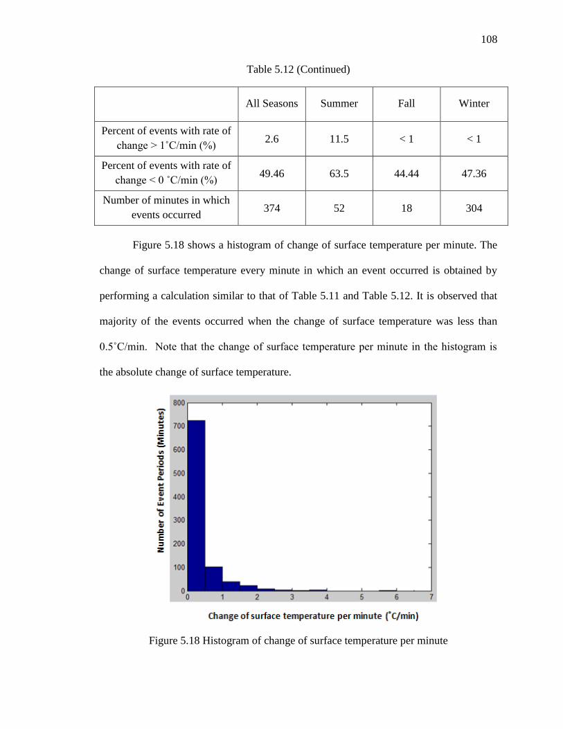
108
Table 5.12 (Continued)
All Seasons Summer Fall Winter
Percent of events with rate of
change > 1˚C/min (%) 2.6 11.5 < 1 < 1
Percent of events with rate of
change < 0 ˚C/min (%) 49.46 63.5 44.44 47.36
Number of minutes in which
events occurred 374 52 18 304
Figure 5.18 shows a histogram of change of surface temperature per minute. The
change of surface temperature every minute in which an event occurred is obtained by
performing a calculation similar to that of Table 5.11 and Table 5.12. It is observed that
majority of the events occurred when the change of surface temperature was less than
0.5˚C/min. Note that the change of surface temperature per minute in the histogram is
the absolute change of surface temperature.
Figure 5.18 Histogram of change of surface temperature per minute

109
Hall (1999) and Hall and Andre (2001) proposed that a rate of change in
temperature equal 2 °C/min was needed to cause cracks in rocks. During this study, a
rate of change in temperature greater than 2˚C/min is commonly observed without
registering an AE event. Additionally, the mean rate of change in surface temperature for
all AE events recorded during the testing period is 0.33 ˚C/min (Table 5.11) and the mean
rate of change in surface temperature during the “dry” AE events recorded during the
testing period is 0.15 ˚C/min (Table 5.11). Both averages are much lower than the
proposed rate of change discussed in the literature.
AE events recorded during dry conditions in the summer had the highest percent
of events with a rate of change in surface temperature greater than 2˚C/min (Table 5.12).
However, it was only 5.8 % of the total dry events observed. Comparatively, 4.7% of all
events recorded during the testing period have a rate of change in surface temperature
greater than 2˚C/min (Table 5.11). The percent of events that have a rate of change in
surface temperature greater than 1˚C/min is also very small (15.2% and 11.5% for all AE
events and for “dry” AE events, respectively). Therefore, the majority of events had a
rate of change in temperature that was less than 1˚C/min. AE events following a rate of
change in temperature as low as 0.0063˚C/min during the winter months (Figure 5.11).
The data from this study demonstrates that the suggested rate of change in temperature
equal to 2 °C/min (Hall, 1999; Hall and Andre, 2001) is not necessarily needed to cause
cracks in rocks.
The majority of events occurred during a decline in temperature. Out of 902
minutes in which AE events occurred, there was a drop in temperature 61.6 % of the
time. Most events occurred during the evening when there was a drop in the overall
temperature of the test specimen due to sunset. Since the majority of AE events occur

110
when there is a drop in temperature, the bottom of the specimen measures the highest
surface temperature and the top of the rock measures the lowest surface temperature (this
trend was discussed in a previous section).
5.2.2.4 Rate of change of maximum – minimum surface temperature
Figure 5.19 displays the difference in surface temperature as a function of time
during a representative 24 hour time period in which events occur during the summer.
The differences in surface temperature (maximum – minimum) are displayed on the
primary axis and number of AE events (indicated by symbols) is displayed on the
secondary axis of Figure 5.19. Similarly, Figure 5.20 and Figure 5.21 display the same
data for the fall and winter seasons, respectively.
On July 21, 2010 (Figure 5.19), events are recorded between from 20:13 to 20:29
and during this time interval, there is a rapid rise in the temperature difference (maximum
–minimum). On September 26, 2010 (Figure 5.20), AE events are recorded between 9
AM and 2 PM and there are rapid rises and falls in the temperature difference. Similarly,
there is a rise in the temperature difference (maximum – minimum) just before the AE
events are recorded on December 18, 2010 (Figure 5.21). Similar trends were observed
on most of the days for which AE events occurred throughout the observation period. In
general, just before an AE event, there is a rapid rise or fall in the surface temperature
difference (maximum – minimum) and the majority of AE events occur during the rising
limb of this difference.

111
Figure 5.19 Difference (maximum-minimum) in surface temperature during AE events in
the summer
Figure 5.20 Difference (maximum-minimum) in surface temperature during AE events in
the fall
AE
Events
AE
Events

112
Figure 5.21 Difference (maximum-minimum) in surface temperature during AE events in
the winter
5.2.3 Effect of Weather on events
The timing of AE events was correlated to the ambient weather conditions using
the weather station data collected during this study. In particular, a large number of AE
events were observed during rains, during a drop in insolation, and during changes in
wind speed and direction. No significant trends were evident from changes in soil
moisture, barometric pressure, or relative humidity as measured by these sensors.
5.2.3.1 Rain
In this study, AE events were observed on most of the rainy days. The presence
of AE events on rainy days may be due to the action of rain drops falling on the test
specimen or they may be caused by the weather conditions affecting the rock conditions
during the rain. If an AE wave was generated due to the sound generated by the impact of
rain drop colliding with the test specimen, the majority of events would be located on the
AE
Events

113
surface of the rock, and the locations would be spread evenly on the surface of the rock
exposed to the rain drops. However, this pattern was not observed (see section 5.2.4
below).
AE events could also be caused by the environmental conditions and changes in
those conditions just prior to or during rain events. For example, on a sunny day just
before a rain, clouds could suddenly move in, cover up the sun, and cause a sudden drop
in temperature on the rock, which could cause cracking. In some cases, some “dry” AE
events were observed immediately before a large number of AE events occurred during
precipitation. Presumably, the “dry” AE events were caused by a change in the
environmental conditions just prior to the rain event.
Since a tipping bucket sensor detects the rain shortly „after‟ it begins, the surface
moisture sensor attached to the rock was utilized to determine if moisture/precipitation
was present. The surface moisture sensor is very sensitive, able to distinguish a few
drops of precipitation on the test specimen. Note that a “dry” surface moisture gage has a
reading less than 200 kOhm while moisture is considered present if the moisture gage has
readings greater than 200 kOhm. This criteria was developed as part of a calibration
exercise in the field. As a result, the surface moisture data was used to categorize “dry”
AE events from all other AE events, and it was possible to distinguish between a “dry”
AE event just before precipitation (resulting from an immediate change in the ambient
conditions) versus AE events that take place minutes later during a rain event.
Figure 5.22 displays precipitation (primary axis) as a function of time during a 24
hour time period on June 24, 2010. Note that precipitation symbols are closed on this
figure. The number of AE events per minute is plotted on the secondary axis. Note that
AE events are open symbols on this figure. For the same date, Figure 5.23 displays

114
surface moisture data (closed symbols) as a function of time. Similar to Figure 5.22,
Figure 5.24 displays precipitation (primary axis) and the number of AE events per minute
as a function of time during a 24 hour time period on December 4, 2010.
Figure 5.22 Precipitation and AE events on June 24, 2010
AE Events (open symbols)
Precipitation

115
Figure 5.23 Surface moisture and AE events on June 24, 2010
On June 24, 2010, a total of 321 AE events were observed (Figure 5.21 and
Figure 5.22). These events were observed from 21:21 to 21:42, from 21:47 to 22:02, at
22:17, at 22:24, from 22:31 to 22:36, at 22:39 and from 22:41 to 22:49. Of those AE
events, a total of 25 “dry” AE events were observed between 21:21 and 21:23 using the
data from the surface moisture sensor (no surface moisture measured). The timing of the
“dry” events (as measured by the surface moisture sensor) indicates that there are “dry”
events observed on a rainy day, and it is assumed that these “dry” events are caused by
sudden changes in weather conditions before the onset of rain. A change in solar
insolation may be one of the ambient conditions that cause the change (discussed in the
following section). In general, the presence of AE events on a rainy day preceded by dry
AE events before the rain is a common trend in all seasons. For this data set, the tipping
AE Events (open symbols)
Surface Moisture (closed symbols)

116
bucket simultaneously detected rainfall at 21:37, 21:42, 22:37, 22:46, 22:51 and 22:59. It
is clear that due to timing issues, the tipping bucket data is not suitable for accurately
distinguishing “dry” versus “wet” AE events each minute, but it is still a critical sensor
that provides information on precipitation events during the day.
Figure 5.24 Precipitaion and AE events on December 4, 2010
Note that on December 24, 2010 (Figure 5.23), there were measurements of
precipitation with no recording of AE events (occurred around 19:30 on Figure 5.23). It
appears that the impact of the rain drop was not strong enough to generate AE waves in
this case. Note that an important observation was made regarding AE events in the
laboratory (prior to field deployment). In the lab, the test specimen was tapped with a
finger, generating only a few AE hits but no AE events. However, when the test specimen
was tapped with a metallic object that generated a more significant sound wave on the
AE Events (open symbols)
Precipitation (closed symbols)
Precipitation (closed symbols)

117
test specimen, a large number of hits were observed, which generated a number of AE
events as defined in this study.
5.2.3.2 Insolation
It is important to note that there is often a drop in insolation preceding a
significant number of AE events. The presence of clouds is the most likely explanation
for a sudden drop in insolation (after sunset, the insolation sensor actually measures
zero). Figure 5.25 displays insolation (closed symbols) as a function of time for a 24
hour time period on June 29, 2010. Figure 5.26 displays precipitation (closed symbols) as
a function of time for a 24 hour time period on the same date. The number of AE events
(open symbols) is displayed on the secondary axis on both these figures.
A total of 59 AE events were observed on June 29, 2010 between 15:29 and
16:40. Three of these AE events were “dry” (observed at 15:29). Figure 5.25 displays a
drop in insolation during the observed AE events. A total of 0.8 mm in precipitation was
recorded between 15:53 and 16:22 in 7 different minute intervals. While precipitation
was recorded at 15:53, the surface moisture sensor indicated a presence in moisture as
early as 15:30 immediately after the three dry events at 15:29. This is a common trend
observed during all seasons. Dry AE events were commonly recorded before wet AE
events so it was hypothesized that these dry AE events were caused by an immediate
change in the surface condition due to an immediate change in insolation.

118
Figure 5.25 Insolation and AE events June 29, 2010
Figure 5.26 Precipitation and AE events on June 28, 2010
Drop in
insolation
AE Events (open symbols)
Insolation (closed symbols)
Measurement of
Precipitation
AE Events (open symbols)
Precipitation (closed symbols)

119
5.2.3.3 Wind speed and wind direction
In addition to the insolation trend discussed in the previous section, there also
appears to be a drop in wind speed and change in wind direction just before or during a
series of AE events. Figure 5.27 displays wind speed (closed symbols) as a function of
time and Figure 5.28 displays wind direction (closed symbols) as a function of time for a
24 hour time period on July 25, 2010. Similar to previous figures, the number of AE
events per minute (open symbols) is displayed on the secondary axis of each figure. A
total of 780 AE events were observed between 20:16 and 20:21. Prior to the AE events
displayed on Figure 5.26, the wind speed was approximately 2 - 3 m/s, and just before the
AE events occurred, the wind speed dropped to less than 0.5 m/s. Similarly on Figure
5.28, the wind direction was approximately 200 to 250 degrees (i.e. South-West) prior to
any AE activity, but the direction changes to 0 to 50 degrees (i.e. North) just before the
AE events occurred. Due to the change in wind direction and wind speed, there could be
a significant change in temperature conditions on the test specimen, which could have
caused the formation of cracks.

120
Figure 5.27 Wind Speed and AE events
Figure 5.28 Wind Direction and AE events
Drop in
wind
speed
Wind Speed (closed symbols)
AE Events (open symbols)
Change in
wind
direction
Wind Direction (closed symbols)

121
5.2.4 Event Location
Figure 5.29 displays an AE event location diagram for all seasons. The ellipsoid
represents the test specimen and the solid dots represent the AE event locations within a 5
cm error of the approximated rock surface. Figure 5.29 (a) and (b) display profile views
(orientation labeled at the bottom of each figure) while Figure 5.29 (c) displays the plan
view.
Figure 5.29 (a) and (b) show that most of the AE events are located in the top
hemisphere of the test specimen. Figure 5.29 (a) indicates that the majority of the events
are located on the east, while Figure 5.29 (b) indicates that majority of the events are
observed towards the south. A large number of cracks are located in the center along the
North-South line as displayed in Figure 5.29(c). These observations are in agreement
with the field data observed by Eppes et al. (2010) and Mc Fadden et al. (2005), but do
not match the suggested results presented by Moores (2008). These results are further
discussed in a subsequent section of this chapter.

122
Figure 5.29 Event locations: (a) profile view (East-West) (b) profile view (North-South)
(c) plan view
5.3 Interpretation of results
Based on the literature review, cracks are formed under a specific set of conditions.
In this section, the results of this study are examined in the context of these conditions
and the hypothesis posed by previous researchers.
5.3.1 Hypothesis 1
The first hypothesis is that cracking occurs due to thermal shock when the rate of
change in temperature of the rock exceeds 2˚C/min (Hall, 1999;Hall and Andre, 2001).
In this study, only 0 to 5.8 % of AE events occur in association with the rate of change of
Test Specimen
South
North
Top Top

123
temperature that exceeds a temperature gradient equal to 2˚C/min (Table 5.11 and Table
5.12 in Section 5.2.2.3). The rate of change in temperatures associated with the AE
activity recorded during this study. Based only on these data, it appears that thermal
shock is not responsible for the majority of cracks. However, McKay et al.,(2009)
demonstrated that rock surface temperatures can change at very high rates on timescales
less than those observed in this study. It is possible that events could be occurring during
periods of high rates of change of temperature that we have not measured with the
temporal resolution of our system
5.3.2 Hypothesis 2
The second hypothesis is that cracking occurs due to cyclic fatigue. The graph in
the Figure 5.8 displays rapid rises and/or falls in surface temperature every minute, but no
events were registered on that day. The maximum rate of change in surface temperature
of 15.89˚C/min and 4.10˚C/min was recorded for the summer and fall seasons,
respectively (Table 5.4). Before any particular event, however, the maximum rate of
change in surface temperature was 5.58˚C/min and 1.99˚C/min, respectively. While the
rates of change in surface temperature on the rock surface may be large enough to cause
cracking, that does not necessarily mean that there will be AE events associated with
those rapid changes. Instead, it could be possible that during a large number of heating
and cooling cycles, cyclic stress is exerted on the rock. Our results suggest that fatigue
might be more important than thermal shock in producing cracks (Figure 5.8). It is only
when the cyclic stress exceeds the fatigue limit of the rock that there is formation or
propagation of cracks.
124
5.3.3 Hypothesis 3
The third hypothesis states that cracks occur due to directional heating and
cooling leading to a preferential north-south direction. The location data (Figure 5.29)
indicate that the cracks are oriented along the north-south direction. This observation is
consistent with the data collected by Eppes et. al (2010) and Mc Fadden et. al. (2005).
However, as discussed in section 5.2.2.2, the largest temperature difference is recorded
between the top and the bottom of the rock, and on the equator, the largest temperature
difference is typically between the north and the south side. Since the largest temperature
difference is along the north-south during the events, the location of the cracks should be
oriented along the east-west line, but in our study cracks are also along the north-south
line.
5.3.4 Hypothesis 4
The fourth hypothesis states that cracks occur due to preferential shading of
certain orientations of preexisting microfractures. The Moores et al. (2008) numerical
model showed that certain orientation of cracks received more insolation than other
cracks. Thus it is hypothesized that cracks which retain water due to lesser solar
insolation propagate preferentially. This hypothesis would lead to an expectation of more
cracks at the bottom than on the top side of the rock since the bottom part of the rock
receives the least amount of insolation. However, the location of events in the Figure 5.29
indicates that there is a prominently larger number of cracks on the top compared to the
bottom. Similar trends are also observed during “dry” AE events. As such, the data do
not support the numerical modeling and hypotheses proposed by Moores et al. (2008).

125
5.3.5 Hypothesis 5
The fifth hypothesis states that cracking occurs due to shock and/or fatigue
associated with a rapid change from cooling to heating (from contraction to expansion)
and/or a rapid change in temperature gradient across the surface of the rock. The results
show that a large number of events occur when there is a sudden change in temperature
caused by either a rapid change in solar insolation due to cloud movement or due to a
change in wind speed or direction. Such a reversal in temperature would cause a rapid
change in surface temperature and, therefore, strain on the rock.
5.3.6 Hypothesis 6
The final hypothesis states that cracking occurs due to processes associated with
water. While a large number of events did occur when the rock was wet, a significant
number of events occurred when the rock was dry (approximately 26.6% of the AE
events recorded). Even when AE events occurred during precipitation, “dry” AE events
often preceded the rain and additional AE events were recorded during the rain event.
Consequently, water may play an important role for propagation of a crack, but it is not
the only factor contributing to it. Temperature variation due to solar insolation and
weather conditions likely causes stress on the rock leading to the formation and
propagation of cracks.

CHAPTER 6: SUMMARY
6.1 Project Summary
The goal of this study was to further investigate the efficacy of insolation on
physical weathering by continuing to modify and improve the rock-instrumentation
established by Garbini (2009). In this study the formation/propagation of cracks as
detected by AE Events was correlated to the temperature, strain and moisture content of
rock. Weather conditions around the test specimen were also studied when AE events
were observed. Various observations during this study either support or refute different
hypotheses (Hall and Andre 2001; Hall and Andre 2003; Hall et al. 2002; McFadden et al.
2005, Halsey et al. 1998; Hallet et al. 1991) on formation of cracks due to insolation.
Overall, the data presented in this study support various hypotheses that suggest that
insolation may play a key role in the breakdown of rocks at Earth‟s surface.
This study was primarily motivated by Earth Science and Civil Engineering-
related questions (i.e. what are the processes responsible for the breakdown of rock and
man-made materials exposed to natural diurnal cycles. In the completion of this work,
however, a number of contributions have been made to the Electrical and Computing
Engineering field of study. In particular, this work represents an extremely novel
application of an embedded electrical system that needed to function under harsh outdoor
conditions. As such, innovations were made to the systems that were unique to its
application. In addition, a novel data analysis technique was developed which could

127
integrate two extremely large datasets using MATLAB programming. The entire study,
therefore, is exemplary of the type of interdisciplinary, application-driven research in the
field of Electrical and Computing Engineering.
6.2 Goals achieved
In this study the following goals were achieved during instrumentation and data
analysis
Eight strain gages, eight thermocouples, six AE sensors, and one surface moisture
sensor was installed on a new test specimen.
A weather station and soil moisture probe was installed on the site to correlate
cracking of rock with the weather conditions.
The strain gage installation technique was improved.
The AE sensor locations on the test specimen and the configuration in the AE Win
software was modified to provide a three dimension location of the AE events to
better study the formation or propagation of cracks.
A wireless modem was installed for continuous remote download of the data.
All data acquisition was powered using solar panels for uninterrupted data
acquisition.
A new data archival and data analysis method was generated using Microsoft excel
spreadsheets in conjunction with MATLAB and C programs.
6.3 Experimental observations
The following observations were made:
The surface temperatures experienced by the rock are similar to those reported for
rocks in desert conditions.

128
Similar to the observation made by McKay (2009), there is a significant difference
between the rock temperature and ambient temperature.
Similar to Garbini (2009), temperature differences exist at different locations on the
rock. The maximum difference is between the top and bottom.
29,541 AE events occurred during 902 minute intervals over 68 days out of 194 days
of observation. 7,834 out of the 29,451 AE events were dry events (no moisture
detected by the surface moisture sensor).
The majority of events occurred during the late afternoon and evening hours just
before and after sunset when the overall surface temperature of the rock is falling.
AE events occur during a full range of temperatures ranging from -7.91˚C to 46.52˚C
so there does not appear to be a unique temperature only condition under which AE
events occur.
In the presence of rain, a large number of AE events were observed due to both a
change in weather conditions before and during the rains as well as the impact of rain
drops on the test specimen.
During many of the AE events, changes in solar insolation, wind speed and wind
direction were observed. These sudden changes can cause thermal shock or thermal
stress fatigue due to change the temperature conditions.
In this study, a rate of change in temperature higher than 2˚C/min is commonly
observed but without registering an event. Up to 5.8 % of AE events had rate of
change in temperature greater 2˚C/min and some events were registered as a result of
a rate of change in temperature as low as 0.0063˚C/min. Hence, a rate of change in

129
temperature equal to 2 °C/min is not necessarily needed to cause cracks in rocks as
suggested by Hall( 1999) and Hall and Andre( 2001).
The abundance of temperature and strain data show that the test specimen underwent
a large number of heating and cooling cycles, likely causing cyclic stress on the rock.
It is possible that cracks are formed when the cyclic stress exceeds the fatigue limit of
the rock.
The majority of AE events were located on the top part of the rock. There were more
events on the east side and toward the north hemisphere in comparison to other
locations. A large number of cracks were found along the north-south line towards the
center.
It is not likely that events are caused by preferential shading of certain fractures as
suggested by Moores et al. (2008) since there were more cracks observed on the top
part of the rock than on the bottom. In accordance with the Moores et al.(2008)
numerical model, the bottom part of the rock should have a larger number of cracks
since the least amount of solar insolation is received at the bottom.
Preferential orientation along the north-south orientation (similar to McFadden et al.
(2005) and Eppes et al. (2010)) was observed, but the temperature data does not show
that it could be due to directional heating and cooling (McFadden et al., 2005, Eppes
et al., 2010).
6.4 Future Work
The major assumption in the data analysis portion of this thesis is that AE events
represent microfracture initiation or propagation in the rock. In order to validate this
assumption, it is recommended that acoustic emission waves be further analyzed. The
amplitude and timing of AE waves during hits and events can be studied in more detail

130
which could help to classify different types of cracks or sources of AE waves. This might
even help us to differentiate between events due to rain drops falling on the test specimen
or other non-crack related phenomenon.
In addition, although various data such as temperature and strain on the rock and
weather conditions around the rock were correlated to timing AE Events, they were not
correlated to the location of events. Modeling (Hallet et al., unpublished) suggests that
cracking would be expected at different locations during different times of day (i.e. on the
rock surface in the evenings and in the interior during mid-day). An analysis of the
location of events by time of day would help to validate such modeling results.
Furthermore, the temperature on different parts of the rock could be examined in more
detail with respect to patterns in wind direction and wind speed that were observed during
AE events. For example, how much temperature change in different parts of the rock is
observed due to change in wind direction?
In addition to these types of analyses on existing data, future rocks of different rock
types or sizes could be instrumented in order to compare and contrast to the data
presented in this study. For example, it is not known if location trends in this rock are
related to heterogeneities of the rock itself or to diurnal forcing of crack events. By
examining additional rocks, such questions could be answered.

131
REFERENCES
Amit, R., Gerson, R., and Yaalon, D.H., 1993. Stages and rate of the gravel shattering
process by salts in desert Reg soils. Geoderma 57, 295–324.
Bahr, H.-A., Fischer, G., Weiss, H.-J., 1986. Thermal-shock crack patterns explained by
single and multiple crack propagation. Journal of Materials Science 21, 2716–2720
Blackwelder, E.B., 1933. The insolation hypothesis of rock weathering. American
Journal of Science 226, 1324-1400.
BURDINE, N. 1963. Rock failures under dynamic loading conditions. Society of
Petroleum Engineers Journal, 3, 1-8.
Cox J. D., Meridith P. G., 1993, Microcrack Formation and Material Softening in Rock
Measured by Monitoring Acoustic Emissions.
Douglas M. Morton (compiler), and Fred K. Miller (compiler), 2003, Preliminary
Geologic Map of the San Bernardino 30' x 60' quadrangle, California: U.S. Geological
Survey Open-File report 03-293, U.S. Geological Survey, Menlo Park, California.
Eberhardt, E., Stead, D., Stimpson, B., and Read, R.S., 1998. Identifying crack initiation
and propagation thresholds in brittle rock. Canadian Geotechnical Journal 35 (2), 222-
233.
Eppes, M.C., McFadden, L., Wegmann, K., and Scuderi, L., 2010. Cracks in desert
pavement rocks: further insights into mechanical weathering by directional solar heating.
Geomorphology 123, 97-108.
Falls, S. D., Chow T., Young Ft. and Hutchins D.Acoustic emission analysis and
ultrasonic velocity imaging in the study of rock failure. J. Acoustic Emission 8, S166-
S169 (1989).
Garbini, J., 2009. Instrumentation and analysis of the diurnal processes affecting a natural
boulder exposed to a natural environment. UNC Charlotte Thesis. 148 p.
Grigg D., 1936. The factor of fatigue in rock exfoliation. Journal of Geology 44, 783-796
Hall, K. and Hall, A., 1996. Weathering by wetting and drying: some experimental
results. Earth Surface Processes and Landforms 21: 365–376.
Hall, K., 1999. The role of thermal stress fatigue in the breakdown of rock in cold
regions. Geomorphology 31, 47–63.
Hall, K., and André, M.F., 2003. Rock thermal data at the grain scale: applicability to
granular disintegration in cold environments. Earth Surface Processes and Landforms 28,
823-836.

132
Hall, K., Andre, M.-F., 2001. New insights into rock weathering from high-frequency
rock temperature data: an Antarctic study of weathering by thermal stress.
Geomorphology 41, 23–35.
Hall, K., Andre, M.-F., 2003. Rock thermal data at the grain scale: applicability to
granular disintegration in cold environments. Earth Surface Processes and landforms 28,
823–836.
Hallet, B., 1983. The breakdown of rock due to freezing: A theoretical model. In:
Proceedings of the 4th International Conference on Permafrost, Fairbanks, Alaska.
National Academy Press, Washington, DC, pp. 433–438.
Hallet, B., Walder, J., and Stubbs., C.W., 1991. Weathering by segregation ice growth in
microcracks at sustained sub-zero temperatures: verification from an experimental study
using acoustic emissions. Permafrost and Periglacial Processes 2, 283-300.
Hardy, H.R., 2003. Acoustic Emission/Microseismic Activity. A.A. Balkema Publishers,
Amsterdam, The Netherlands. 297 p.
Hayashi, M., Kanagawa T., Hibino S., Matojima M.and Kitahara Y. Detection of
anisotropic geostresses trying by acoustic emission, and non-linear rock mechanics on
large excavating caverns. In Proc., 4th
Congress Internat. Soc. for Rock Mechanicson
Rock Mechanics pp. 212-218. Montreaux, Switzerland (1979).
Hoerlé, S., 2006. Rock temperatures as an indicator of weathering processes affecting
rock art. Earth Surface Processes and Landforms 31, 383–389.
Hoerlé, S., 2006. Rock temperatures as an indicator of weathering processes affecting
rock art. Earth Surface Processes and Landforms 31, 383–389.
Holcomb, D. J. and Costin L. S. Detecting damage surfaces in brittle materials using
acoustic emissions. J. Appl. Mech. 108,536-544 (1986).
Holcomb, D. J. Using acoustic emissions to determine in-situ stress: problems and
promise. Geomechanics, ASME, AMD 57, 11-21 (1983).
Khair, A., 1981. Acoustic emission pattern; an indicator of mode of failure in geologic
materials as affected by their natural imperfections. Acoustic Emission/Microseismic
Activity in Geologic Structures and Materials; proceedings of the third conference, 45-
66.
Kranz, R. L., Satoh T., Nishizawa O., Kusunose K.,Takahashi M., Masuda K. and Hirata
A. Laboratory study of fluid pressure diffusion in rock using acoustic emissions. J.
Geophys. Res. 95, 21,593-21,607 (1990).
Lei X., Kusunose, K., Rao, M., Nishizawa, O., and Satoh, T., 2000. Quasi-static fault
growth and cracking in homogeneous brittle rock under triaxial compression using
acoustic emission monitoring. Journal of Geophysical Research 105, 6127-6139.

133
Lockner, D. A. and Byerlee J. D. Hydrofracture in Weber sandstone at high confining
pressure and differential stress. J. Geophys. Res. 82, 2018-2026 (1977).
Lockner, D. A., Byerlee J. D., Kuksenko V., Ponomarev A. and Sidorin A. Quasi-static
fault growth and shear fracture energy in granite. Nature 350, 39-42 (1991).
Lord, A. E. J. and Koerner R. Acoustic emissions in geological materials. In
Fundamentals of Acoustic Emission (Edited by K. Ono), pp. 261-307. Materials Dept.,
UCLA, Los Angeles (1978)
Matsuoka, N., 1991. A model of the rate of frost shattering: Application to field data
from Japan, Svalbard and Antarctica. Permafrost and Periglacial Processes 2, 271–281.
Matsuoka, N., Moriwaki, K., Iwata, S., Hirakawa, K., 1990. Ground temperature regimes
and their relation to periglacial processes in the Sør Rondane Mountains, East Antarctica.
Proceedings of the National Institute of Polar Research Symposium on Antarctic
Geosciences 4, 55–66.
McFadden, L.D., Eppes, M.C., Gillespie, A.R., and Hallet, B., 2005. Physical weathering
in arid landscapes due to diurnal variation in the direction of solar heating. Geological
Society of America Bulletin 110, 161–173.
McGreevy, J.P., 1985. Thermal properties as controls on rock surface temperature
maxima, and possible implications for rock weathering. Earth Surface Processes and
Landforms 10, 125–136.
McKay, C.P., Molaro, J.L., and Marinova, M.M., 2009. High-frequency rock temperature
data from hyper-arid desert environments in the Atacama and the Antarctic Dry Valleys
and implications for rock weathering. Geomorphology 110, 182–187.
Molaro, J. L. and McKay, C. P., 2010. Processes controlling rapid temperature variations
on rock surfaces. Earth Surface Processes and Landforms 35, 501–507.
Moores, J.E., Pelletier, J.T., and Smith, P.H., 2008. Crack propagation by differential
insolation on desert surface clasts. Geomorphology 102, 472-481.
Moores, J.E., Pelletier, J.T., and Smith, P.H., 2008. Crack propagation by differential
insolation on desert surface clasts. Geomorphology 102, 472-481.
Nicholson, D.T., 2001. Pore properties as indicators of breakdown mechanisms in
experimentally weathered limestones. Earth Surface Processes and Landforms 26, 819–
838.
Nishizawa, O., Onai K. and Kusunose K. Hypocenter distribution and focal mechanism
of AE events during two stress stage creep in Yugawara andesite. Pure Appl. Geophys.
122, 36-52 (1984).

134
Nordlund, E. and Li C. Acoustic emission and the Kaiser effect in rock materials. In
Proc., 31st U. S.Rock Mechanics Symposium (Edited by W. A. Hustrulid and G. A.
Johnson), pp. 1043-1050. Balkema, Rotterdam (1990).
Obert, L. and DuvaU W. U.S. Bureau of Mines, Rept.Invest. RI-3654, (1942).
Obert, L. U.S. Bureau of Mines, Rept. Invest. RI-3555, (1941).
Ødeg°ard, R.S., Sollid, J.L., 1993. Coastal cliff temperatures related to the potential for
cryogenic weathering processes, western Spitsbergen, Svalbard. Polar Research 12, 95–
106.
Rao N., Murthy, G., and Raju, N., 1998. Characterization of micro and macro-cracks in
rocks by acoustic emission. ASTM Special Technical Publication 1353, 141-155.
Scholz, C. H. Experimental study of the fracturing process in brittle rocks. J. Geophys.
Res. 73, 1447- 1454 (1968).
Shiraiwa, T., 1992. Freeze–thaw activities and rock breakdown in the Langtang Valley,
Nepal Himalaya. Environmental Science, Hokkaido University 15, 1–12.
Sondergeld, C. H. and Estey L. H. Acoustic emission study of microfracturing during the
cyclic loading of Westerly granite. J. Geophys. Res. 86, 2915-2924(1981).
Sondergeld, C. H. and Estey L. H. Source mechanisms and microfracturing during
uniaxial cycling of rock. Pure Appl. Geophys. 120, 151- 166 (1982).
Sondergeld, C. H., Granryd L. A. and Estey L. tt.Acoustic emission during compression
testing of rock. In 3rd Conf. on Acoustic Emission/Mieroseismic Activity in Geol.
Str~ctures and Materials (Edited by H. R. Hardy and W. F. Leighton), pp. 131 145.
Trans-Tech. Publications, Clausthal-Zellerfeld, Germany (1984).
Strini, A., Guglielmin, M., Hall, K., 2008. Tafoni development in a cryptic environment:
an example from Northern Victoria Land, Antarctica. Earth Surface Processes and
Landforms 33, 1502–1519.
Sumner, P.D., Meiklejohn, K.I., Nel, W., Hedding, D.W., 2004. Thermal attributes of
rock weathering: zonal or azonal? A comparison of rock temperatures in different
environments. Polar Geography 28, 79–92.
Tanigawa, Y., and Takeuti, Y., 1983. Three-dimensional thermoelastic treatment in a
spherical region and its application to solid sphere due to rotating heat source: Zeitschrift
fur angewandte mathematik und mechanik 63, 317–324.
Turkington, A., 2005. Stone Decay in the Architectural Environment. Geological Society
of America Special Publication 390, 62 p.
Van Hise, C. R., 1904 A Treatise on Metamorphism. U. S. Geo. Survey Viles, H.A. and
Goudie, A.S., 2007. Rapid salt weathering in the coastal Namib Desert: Implications for
landscape development. Geomorphology 85, 49-62.

135
Viles, H.A., 2005. Microclimate and weathering in the central Namib Desert.
Geomorphology 67, 189-209.
Walther, Johannes, 1924, Dad Gesetz der Wüstenbildung. Ed 4.
Wegmann, M., and Gudmundsson, G.H., 1999. Thermally induced temporal strain
variations in rock walls observed at subzero temperatures. Lecture notes in Physics, 533:
511-518.
Yanagidani, T., Ehara S., Nishizawa O., Knsunose K.and Terada M. Localization of
dilatancy in Ohshima granite under constant uniaxial stress. J. Geophys. Res. 90, 6840-
6858 (1985).
Yatsu, E., 1988. The Nature of Weathering: An Introduction. Sozosha, Tokyo. 624 pp.