1

Nationwide and State-by-State Emission Benefits of a

Gasoline Sulfur Limit

Thomas L. Darlington

Jeremy G. Heiken

Dennis Kahlbaum

Air Improvement Resource, Inc.

47298 Sunnybrook Lane

Novi, Michigan

48374

ABSTRACT

EPA recently completed its study of the need, cost-effectiveness, and

technological feasibility of Tier 2 standards, and will soon propose Tier 2 standards for

cars and light trucks. As a part of its Tier 2 Study and the upcoming Tier 2 notice of

proposed rulemaking (NPRM), EPA is also studying the effects of gasoline fuel sulfur on

exhaust emissions from advanced technology vehicles, and has indicated it will

implement some kind of sulfur limit in gasoline as well. Both the American Automobile

Manufacturers Association (AAMA) and the American Petroleum Institute (API) have

forwarded proposals for reducing sulfur in gasoline. This analysis examines these

proposals and examines the emission data on the effect of sulfur on advanced technology

and current vehicles. An advanced MOBILE5 model was created to incorporate a number

of recent improvements in emission factor methodology and to include the effects of

sulfur on exhaust emissions for different vehicle technologies. Finally, the model was

used with activity data obtained from EPA to determine nationwide, and state-by-state

emission reductions of HC, CO, NOx, and PM for the two proposals. The results of the

analysis indicates that the emission reductions from the AAMA proposal exceed the API

proposal and that low sulfur fuel appears to be essential to achieve the full emissions

benefit from advanced national LEV vehicles (NLEVs) and Tier 2 vehicles.

INTRODUCTION

EPA recently published its Tier 2 Study to Congress, which outlined the need for,

the cost effectiveness, and the technological feasibility of Tier 2 standards for cars and

light trucks. (1) EPA presented evidence in the Study, which indicated that, in EPA’s

view, additional reductions in vehicle emissions are needed, that technologies exist with

which to lower vehicle emissions, and that these technologies appear to be cost effective.

The Study further indicated that EPA intends to establish these same items with respect to

the Tier 2 standards by notice of proposed rulemaking and that this NPRM would be

released early next year (1999).

2

EPA further indicated in the Study that, as a part of the Tier 2 rulemaking process,

EPA would consider whether gasoline sulfur controls were needed as well as lower

vehicle standards. EPA concluded that “sulfur in gasoline affects emissions of HC, CO,

and NOx by inhibiting the performance of the catalyst,” and that “recent information

from test programs...suggest that not only do LEV and Tier 1 vehicles exhibit decreased

emissions performance due to fuel sulfur, but the more advanced the technology, the

more sensitive (on a percentage basis) the catalysts are to sulfur.” Prior to the release of

the Final Tier 2 Study, EPA released a report on gasoline sulfur issues, which covered

more detail concerning sulfur’s effects on vehicle emissions. (2)

The American Society of Testing Materials (ASTM) sets minimum specifications

for a number for gasoline properties, including sulfur. The ASTM specification for

maximum sulfur content in the U.S. is 1000 ppm. (3) The State of California controls

gasoline sulfur levels directly. California’s Phase 2 reformulated gasoline requirements

(RFG), implemented in 1996, establish a sulfur cap limit of 80 ppm, a flat limit of 40

ppm, and an averaging limit of 30 ppm. (4) These requirements are substantially below

the U.S. national average sulfur value of 339 ppm, as used by EPA’s on-highway

emissions model, MOBILE5B, and in the Complex Model. (5) The State of Georgia also

has a rule in place reducing sulfur in 25 counties. The rule calls for a two-step reduction

of 150 ppm average starting on April 1, 1999, and 30 ppm average starting on April 1,

2003. (6)

EPA also established reformulated gasoline (RFG) requirements, but these

requirements stopped short of specifying a sulfur limit. Instead, Federal RFG is a

performance specification of a 15% reduction in VOC in 1995, followed by a further

10% reduction (for a total of 25%) in 2000. (7) Fuel suppliers will use EPA’s Complex

Model for determining the optimum and lowest cost specification needed to meet the

25% reduction. EPA expects that on average, Federal Phase 2 reformulated gasoline will

have a sulfur level of around 150 ppm. (2) However, in some cases, the sulfur level with

Phase 2 could be substantially higher. Also, there is a concern with the Complex Model,

because the emission effects are based on 1990 technology vehicles, and not on advanced

technology National Low Emission Vehicles (NLEVs) or Tier 2 vehicles, which could

have significantly lower emission standards than NLEVs.

In March 1998, the National Low Emission Vehicle program was adopted by

EPA, 46 States outside of California, and the automobile manufacturers. (8) In this

program, the automobile manufacturers will provide California vehicles in the Ozone

Transport region starting in 1999, and the remainder of the 45 states in 2001. New York,

Massachusetts, Maine, and Vermont did not opt-into the program because these states

have implemented the California vehicle standards in various years. Thus, all states in the

U.S. will have advanced technology vehicles no later than 2001. Shortly after the NLEV

program was implemented, the American Automobile Manufacturers Association

(AAMA) petitioned EPA to reduce the sulfur in gasoline year-round, on a nationwide

basis, to the same specifications as California’s sulfur specifications, citing numerous

studies showing the negative impacts of sulfur on emissions from current and advanced

technology vehicles. (9)

3

Partly in response to AAMA’s petition and the Tier 2 Vehicle and Gasoline Sulfur

Studies, the American Petroleum Institute forwarded their proposal for reducing sulfur.

(10) The API proposal is basically a two-phase proposal in which sulfur is reduced in 22

OTAG states and 7 other states in 2004, and further reduced if needed in areas with

Federal Phase 2 reformulated gasoline in 2010. More will be presented on both the

AAMA and API proposals in the Methodology section.

To put these proposals in perspective, this analysis examines the nationwide and

state-by-state emission benefits of the two proposals using recent evidence of the effect

of sulfur on advanced technology vehicles. The analysis first examines sulfur levels

across the U.S. using recent service station data obtained by AAMA. Next, the analysis

examines recent test data on the effects of sulfur levels on advanced technology (LEV)

vehicles. The analysis then discusses modifications made to the MOBILE5B model to

estimate the effects of sulfur on vehicle emissions. Finally, the analysis presents the

results of using this model to estimate the emission benefits of both proposals.

METHODOLOGY

Examination of Current Gasoline Sulfur Levels In the U.S.

The AAMA conducts a semi-annual survey of motor vehicle fuels in various

cities in the U.S. and Canada. Each winter and summer, samples of gasoline and diesel

fuel are taken from service stations and analyzed for numerous properties. One of the

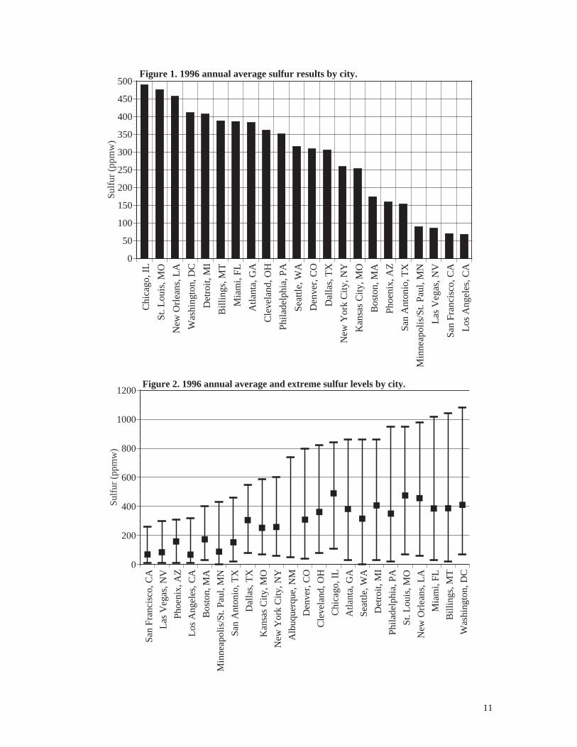
properties analyzed is sulfur content. AIR obtained the 1996 survey from AAMA , which

contains about 800 samples, and analyzed the data by city for premium, mid-grade, and

regular combined. (11) The results are shown in Figure 1.

The figure shows a wide variation in average sulfur levels across the U.S. The

averages range from a high of almost 500 ppm in Chicago, to a low of around 60 ppm in

Los Angeles. The California values are higher in 1996 than the California sulfur standard

because Phase 2 reformulated gasoline did not take effect until the Spring of 1996, and

this survey includes winter samples in California, which were not yet subject to the sulfur

requirement. The summer, 1996 average for California was below 30 ppm. Outside of

California, the lowest average appears to be in the Minneapolis area. Figure 2 shows

extreme values for the same cities, rank-ordered by city by the highest sulfur level. Two-

thirds of the cities in this survey have extreme values that exceed 500 ppm.

Sulfur Proposals

Table 1 outlines the AAMA and API proposals for reducing sulfur in U.S.

gasoline. The AAMA proposal calls for a year-round sulfur average of 30 ppm and a cap

of no more than 80 ppm, in the entire U.S., starting on January 1, 2004. This is consistent

with California’s Phase 2 reformulated gasoline specification for sulfur. The API

proposal is in two phases. Phase 1 starts in 2004, or with the introduction of Tier 2

vehicles, whichever is later. There are basically two standards in Phase 1. The more

4

stringent sulfur specification covers the 22 OTAG states in EPA’s NOx SIP Call, and

New Hampshire, Vermont, Mississippi, Florida, Louisiana, and East Texas. This

specification is a sulfur average of 150 ppm with a 300 ppm cap. The less stringent sulfur

specification applies to the remainder of the states in 2004, and includes a 300 ppm sulfur

average and a 450 ppm cap. Phase 2 starts in 2010, if necessary (API’s Phase 2 proposal

calls for a study to be conducted by EPA to determine the need for the Phase 2

standards), and includes a sulfur average of 30 ppm and a cap of 80 ppm, in the same

states that have 150 ppm above. The non-RFG states in Phase 2 of the API proposal

would continue with the sulfur requirements as in Phase 1.

Vehicle Emission Response to Gasoline Sulfur Level

Sulfur’s impact on catalytic activity has been studied extensively for the past ten

years. Sulfur’s impact on emissions is included in EPA’s MOBILE5B model, in the EPA

COMPLEX Model for fuels, in California’s on-highway model MVEI7G, and in

California’s Predictive Fuels Model (similar to EPA’s COMPLEX Model). For this

analysis we are interested in sulfur’s effects on three basic groups of vehicles:

• Tier 0 vehicles, or those built between 1981and 1994

• Tier 1 vehicles, built between 1994 and 2001

• Low Emission Vehicles (LEVs), or those built starting in 2001 (1999 in the Ozone

Transport Region)

The EPA Complex Model is based on tests of 1990 technology vehicles, therefore,

the emissions response to sulfur in this model is appropriate for Tier 0 vehicles. To

obtain this response, AIR ran the Phase 2 COMPLEX Model at different sulfur levels for

HC, CO, and NOx, using both high- and low-emitters, and plotted the results. This is

shown for HC and NOx in Figure 3. The results show that reducing sulfur from 339 ppm

to 30 ppm would reduce exhaust HC by about 6% and NOx by about 12%.

For Tier 1 vehicles, AIR obtained test data from the Auto/Oil testing. Six Tier 1

vehicles were tested on two fuels that contained 40 ppm and 330 ppm sulfur. For newer

technology vehicles, the emissions data are generally linear when plotted on a log-log

basis, that is, there is good correlation when a linear regression is fitted through the log

of emissions and the log of the sulfur value. AIR used this relationship to characterize

the emissions data for Tier 1 vehicles. For NOx, the sulfur sensitivity was similar to Tier

0 vehicles, but for HC, the sulfur sensitivity was higher than for Tier 0 vehicles. The Tier

1 response to sulfur is shown in Figure 4.

For LEV vehicles, there have been two recent testing programs conducted to

estimate the emission effects. One was conducted by AAMA and the Association of

International Automobile Manufacturers (AIAM), and a second one by CRC. In the

AAMA/AIAM program, 12 production and production-intent LEV and ULEV light duty

vehicles and 9 LEV and ULEV light duty trucks were tested at fuel sulfur levels of 40,

100, 150, 330, and 600 ppm sulfur. All vehicles were equipped with aged components to

simulate 100,000 miles. (12) In the CRC program, 12 1997 passenger cars were tested on

5

the same fuels as above. (13) The two programs yielded very similar results. For this

analysis, AIR utilized the AAMA/AIAM program data. AIR again regressed the log of

emissions versus the log of sulfur for cars and light trucks combined, and obtained the

relationships shown in Figures 5 and 6. Figures 5 and 6 also show the relationship for

Tier 1 and Tier 0 vehicles. Emissions for the curves have been normalized to a value of

1.0 at 339 ppm sulfur. For HC (Figure 5), the curves show that LEVs are more sensitive

to sulfur than Tier 1 vehicles, and Tier 1 vehicles are more sensitive than Tier 0 vehicles.

For NOx (Figure 7), the curves show that Tier 0 and Tier 1 vehicles appear to display

about the same sensitivity on a percentage basis, whereas LEVs appear to be much more

sensitive.

There is yet another way to view this data. LEVs are certified on California Phase

2 gasoline with a sulfur level of about 30 ppm. Their HC emissions are typically 0.04-

0.05 g/mi, and the NOx levels are 0.07-0.12 g/mi. When these vehicles are sold in the 49-

States, however, they operate on fuels with sulfur values as high as 500-800 ppm. At

about 350 ppm, the curves in Figures 6 and 7 would indicate that HC emissions are on

average about 35% higher, and NOx emissions are about 140% higher. Thus, much of the

benefit of these Low Emission Vehicles is being lost because of operation on higher

sulfur fuels.

Reversibility of Sulfur Effect

Reversibility refers to the ability of the catalyst to recover to full or near-full

conversion capability on low sulfur fuel after experiencing. This is a very key issue in the

debate concerning the API proposal. The API proposal calls for different sulfur levels in

different areas. If advanced technology vehicles with advanced catalysts are not

completely reversible, then vehicles that travel from a low sulfur region to a higher sulfur

region and back will have higher emissions than those that never travel to a higher sulfur

region. Conversely, if the effects are completely reversible, then traveling from region-to-

region and vehicle migration issues are less important when comparing the two

proposals.

According to EPA’s Gasoline Sulfur Report, some vehicles appear to be

reversible while others do not. The reversibility is related in part to the presence of some

rich operation: rich operation tends to clear out the sulfur dioxide which is stored on the

catalyst, reducing its effectiveness. Advanced technology vehicles such as LEVs with

off-cycle controls will have less rich operation under normal circumstances due to EPA’s

and the Air Resources Board’s off-cycle controls. Therefore, advanced technology

vehicles with off-cycle controls may have less reversibility than today’s vehicles.

Currently, testing is nearly completed by the Coordinating Research Council on

sulfur reversibility. This data will be analyzed extensively in the coming months. This

analysis makes the most optimistic assumption that sulfur effects are completely

reversible. This is only an assumption at this point, it is not based on any AIR analysis of

the reversibility data. As such, the emission benefits of the API proposal as presented in

this paper would be less than estimated if the sulfur effect were not completely reversible.

6

The relationships used in Figures 5 and 6 were used to develop correction factors

for use in the MOBILE5 model. This will be discussed in more detail in the next section.

HC and NOx Modeling Using Modified MOBILE5B

Over the last two years, there has been a significant amount of work performed by

AIR, EPA and others on changes to MOBILE5 for MOBILE6. Much of this work was

unpublished until recently, but as a part of the Tier 2 Study, EPA created a new model,

called the “Tier 2 Analysis Tool”, or “Modified MOBILE5B” (which we will call

MM5B) in which major changes have been made to the emission model. (1) These have

occurred in four major areas:

• Add off-cycle emissions (both aggressive driving and air conditioning effects),

• Incorporate lower deterioration for Tier 0, Tier 1 and LEV vehicles, particularly in

areas without enhanced I/M programs,

• Incorporate higher light duty truck VMT fractions, and

• Incorporate fuel sulfur effects

EPA’s MM5B changes are detailed in Appendix A of the Tier 2 Study.

AIR also has a MM5B, which is very similar but not exactly equivalent to EPA’s

MM5B, which AIR has used extensively to demonstrate the incremental emission effects

of some of these changes. The differences in AIR’s MM5B and EPA’s MM5B are (1)

somewhat different off-cycle effects, (2) slightly lower light truck VMT fractions in the

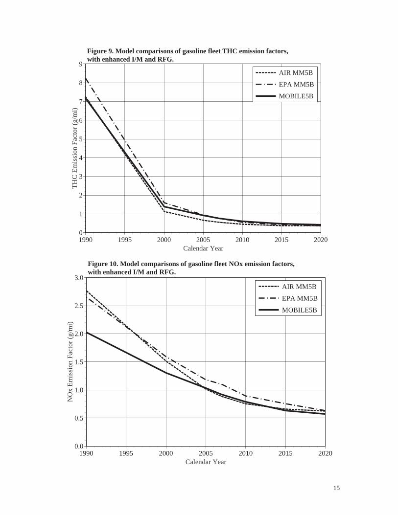
AIR model, and (3) slightly different fuel sulfur effects. Figures 7 – 10 present a

comparison of EPA’s MOBILE5B model, and EPA’s and AIR’s MM5B models for

gasoline vehicles only. The modified models include the four changes listed above, where

MOBILE5B was run in the stock configuration. All other inputs were the same. Figures 7

and 8 show HC and NOx emissions for areas without I/M or RFG. Figures 9 and 10 show

HC and NOx emissions for areas with enhanced I/M and RFG. As shown in the figures,

AIR’s and EPA’s models are similar, and both appear to be different from MOBILE5B.

The primary item to note from Figures 7 - 10 are that the modified models have generally

higher emissions in the early 1990s, and somewhat lower emissions in the 2005+ time

frame, than the current MOBILE5B model (except for NOx with enhanced I/M and RFG,

where the different models appear to be about equivalent). Early 1990s emissions are

higher due to the addition of off-cycle effects. The 2005+ emissions are lower in non-

I/M areas due to lower deterioration and off-cycle regulations. The increased VMT

fractions of light duty trucks mitigate the reductions somewhat, because LDTs are

certified to somewhat higher standards than cars because of their use patterns.

For this analysis, AIR used its MM5B to estimate the emission reductions of the

two proposals. AIR’s model includes the four modifications mentioned above. For the

sulfur effects, AIR modified the model to accept a sulfur content as an input variable, and

placed sulfur correction factors for the various vehicle technologies (Tier 0, Tier 1 and

LEV) in the block data to the program. Since the test data developed the relationship of

7

emissions to sulfur level on the basis of full Federal Test Procedure (FTP) values

(including cold start, stabilized, and hot start driving), the sulfur adjustment factors were

applied to FTP-based exhaust emissions. The model therefore makes all of the

subsequent adjustments to exhaust emissions automatically. All counties without RFG

were assumed to have a baseline sulfur value of 339 ppm (same as national average), and

all counties with RFG were assumed to have a nominal sulfur value of 150 ppm.

For vehicle technology, we assumed the NLEV program starting in 2001 for cars and

light trucks from 0-6,000 lbs. GVW. For the other MOBILE5B inputs, we assume the

following:

• Vehicle speed of 28 mph

• Ambient temperature of 75o F

• Diurnal temperature of 60o F to 84

o F

• Operating mode mix of 20.6/27.3/20.6

• Basic and enhanced I/M inputs were standard EPA default values

Particulate Matter Modeling Using PART5

AIR used PART5 to estimate PM reductions due to the proposals. (14) PART5

estimates directly emitted particulate emissions (carbonecous and sulfates), as well as

brake and tire wear, and indirect sulfates formed from atmospheric reactions of SO2. The

base model incorporates the Tier 1 vehicle standards, but not the effect of the NLEVs.

Since NLEVs have low HC emissions, these vehicles might be expected to have slightly

lower directly emitted carbonecous PM. Omitting these vehicles from the PM analysis,

however, would not significantly affect the relative benefits of the two proposals. To

estimate PM emissions from the proposals, this analysis computed the gasoline vehicle

weighted-average emission rates at the different sulfur levels.

The PART5 model assumes that 12.0 % of the SO2 reacts in the atmosphere to

form indirect sulfate PM.

Vehicle Activity and Other Input Information

To estimate nationwide and state-by-state benefits of the proposals, AIR obtained

vehicle miles traveled (VMT) information by state and county from Pechan and

Associates for calendar year 2007, which has been used by EPA in its National Emissions

Data System (NEDS). This information also included I/M program and reformulated

gasoline status by county. From this information, AIR was able to determine the

nationwide, and state-by-state vehicle miles traveled for six different types of areas in the

nation, as shown in Table 2. This information was also developed for each state.

To predict VMT for other years, AIR reviewed the OTAG growth rates by state,

and estimated that the population-weighted average growth rate was about 1.9% over the

period from 1990 to 2007. For this analysis, we assumed a 2% growth rate for every state

8

and for the nation, and estimated VMT in years prior to 2007 by subtracting 2% per year,

and for years after 2007 by adding 2% per year.

RESULTS

Nationwide Emission Benefits

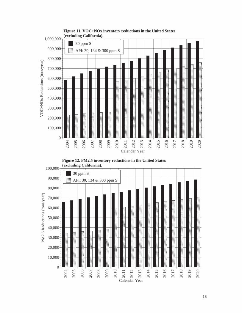
Using the above model, nationwide VOC and NOx emission benefits in tons per

year are shown in Figure 11. This chart includes NLEVS starting in 2001, and their

increased sensitivity to high sulfur fuel. The analysis assumes that the baseline sulfur

level in all non-RFG areas is 339 ppm, and in all RFG areas is 134 ppm. VOC and NOx

emission reductions due to the AAMA proposal (30 ppm) start at almost 600,000 tons per

year in 2004, and increase to almost a million tons per year in 2020, assuming 2%

growth. For the API proposal, VOC + NOx emission reductions start at about 220,000

tons per year in 2004, and increase to about 750,000 tons per year in 2020. The API

proposal improves in 2010 when all of states east of the Mississippi are assumed to have

low sulfur fuel. In this case, we have assumed that, under the API proposal, EPA’s study

finds that low sulfur is needed. In the event low sulfur fuel is not needed, the benefits of

the API proposal would be much less.

PM2.5 emission reduction benefits using the PART5 model are shown in Figure

12. As noted earlier, the PART5 model assumes that 12% of the SO2 from the vehicle

exhaust reacts to form sulfate PM in the atmosphere, on average. This figure would vary

widely by geographic location and meteorological conditions. The primary and secondary

PM reductions have been summed in Figure 12. Once again, the AAMA proposal shows

more significant PM reductions than the API proposal.

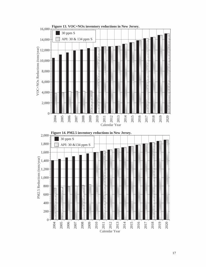
Example State Benefits

We have included similar charts for two very different states – New Jersey and

Oklahoma. New Jersey is assumed to have 100% enhanced I/M and reformulated

gasoline, and Oklahoma has no I/M or RFG. Figure 13 shows VOC and NOx reductions

in New Jersey. In 2004-2010, the AAMA proposal results in much lower emissions. In

2010, however, the API proposal would be equivalent to the AAMA proposal, if EPA’s

Study finds that sulfur control is needed. PM emission reductions in New Jersey are

shown in Figure 14.

Figure 15 shows HC and NOx emission reductions in Oklahoma. In Oklahoma,

the API proposal results in small emission reductions, because the sulfur level is assumed

to be reduced from 339 ppm to only 300 ppm., even after 2004 The AAMA proposal,

however, results in much more significant reductions. Figure 16 shows PM2.5 reductions

in Oklahoma.

9

DISCUSSION

In this analysis, we have developed new relationships of the influence of gasoline

sulfur on Tier 1 and LEV emissions, and applied those to an updated MOBILE5B model.

In this process, there are some uncertainties that could have an influence over the size of

the emission reductions in each case. A few of these are:

• The second phase of the API proposal is contingent on EPA finding that lower sulfur

fuel is necessary. If EPA finds it is not necessary, the reductions due to the API

proposal would be significantly less in the post-2004 timeframe.

• If advanced technology vehicles with off-cycle controls exhibit less reversibility, the

benefits of the API proposal would be less also.

The following effects would affect the magnitude of benefits from both programs, but

would not affect the relative differences between the two programs.

• We have assumed that the car and trucks response can be estimated by combining the

car and light trucks sulfur data. The EPA Gasoline Sulfur report indicates that trucks

may have a somewhat less significant response to sulfur than cars. However, since

this analysis was based on both sets of vehicles, this is already factored into the

analysis.

• We have assumed that same response for both normal and high emitters. The

COMPLEX model separates these responses for Tier 0 vehicles. This is also not

thought to be a significant factor, because Tier 1 and LEV vehicles are equipped with

California onboard diagnostics (OBD2), which should for most vehicles, keep the

emissions quite low. Furthermore, Tier 1 and NLEV vehicles that are higher emitters,

are not expected to be nearly as high emitting as some of the high emitting Tier 0

vehicles.

• We have assumed that all conventional gasoline states have a baseline gasoline sulfur

content of 339 ppm. However, it was shown early in this analysis that there is

significant variation in sulfur content by city.

CONCLUSIONS

EPA is in the process of deciding on Tier 2 vehicle standards for cars and light

trucks. As a part of the Tier 2 standards process, EPA is also considering reducing sulfur

in gasoline. AAMA and API have both forwarded proposals for reducing sulfur in the

U.S. This analysis examined the relative emission reductions of the two proposals for

HC, NOx and PM. The study found that the AAMA proposal provides more significant

reductions in HC, NOx, and PM than the API proposal.

10

Table 1. Comparison of AAMA and API Proposals

Sulfur (ppmw) Source

Average Cap

Season Geographical Coverage Year

AAMA 30 80 All Entire U.S. 2004

150 300 All 22 OTAG States + ME,

NH, VT, MS, FL, LA, East

TX

2004 API Phase 1

300 450 All Remainder of States 2004

API Phase 2 30 80 All Same States that receive

150 ppm above

2010

Table 2. 2007 VMT by I/M and RFG Status

I/M and RFG Status VMT (106 miles per year) VMT (%)

No I/M, No RFG 1,430,685 52.5%

No I/M, Federal RFG 48,527 1.8%

Basic I/M, No RFG 346,119 12.7%

Basic I/M, RFG 38,103 1.4%

Enhanced I/M, no RFG 284,713 10.4%

Enhanced I/M, RFG 548,713 21.2%

11

Chi

cago

, IL

St. L

ouis

, MO

New

Orle

ans,

LAW

ashi

ngto

n, D

CD

etro

it, M

IB

illin

gs, M

TM

iam

i, FL

Atla

nta,

GA

Cle

vela

nd, O

HPh

ilade

lphi

a, P

ASe

attle

, WA

Den

ver,

CO

Dal

las,

TXN

ew Y

ork

City

, NY

Kan

sas C

ity, M

OB

osto

n, M

APh

oeni

x, A

ZSa

n A

nton

io, T

XM

inne

apol

is/S

t. Pa

ul, M

NLa

s Veg

as, N

VSa

n Fr

anci

sco,

CA

Los A

ngel

es, C

A

0

50

100

150

200

250

300

350

400

450

500

Sulfu

r (pp

mw

)

Figure 1. 1996 annual average sulfur results by city.

San

Fran

cisc

o, C

ALa

s Veg

as, N

VPh

oeni

x, A

ZLo

s Ang

eles

, CA

Bos

ton,

MA

Min

neap

olis

/St.

Paul

, MN

San

Ant

onio

, TX

Dal

las,

TXK

ansa

s City

, MO

New

Yor

k C

ity, N

YA

lbuq

uerq

ue, N

MD

enve

r, C

OC

leve

land

, OH

Chi

cago

, IL

Atla

nta,

GA

Seat

tle, W

AD

etro

it, M

IPh

ilade

lphi

a, P

ASt

. Lou

is, M

ON

ew O

rlean

s, LA

Mia

mi,

FLB

illin

gs, M

TW

ashi

ngto

n, D

C

0

200

400

600

800

1000

1200

Sulfu

r (pp

mw

)

Figure 2. 1996 annual average and extreme sulfur levels by city.

12

0.0

0.2

0.4

0.6

0.8

1.0

1.2

1.4

1.6

0 100 200 300 400 500 600 700 800 900 1000

Emis

sion

s (g/

mi)

Sulfur (ppmw)

Exhaust HC

Exhaust NOx

Figure 3. Emissions versus sulfur, EPA Complex Model.

0.00

0.05

0.10

0.15

0.20

0.25

0.30

0.35

0 100 200 300 400 500 600 700 800 900 1000

Emis

sion

s (g/

mi)

Sulfur (ppmw)

Exhaust HC

Exhaust NOx

Figure 4. Emissions versus sulfur, Tier1 vehicles.

13

0.70

0.75

0.80

0.85

0.90

0.95

1.00

1.05

1.10

0 100 200 300 400 500 600

Rat

io, e

mis

sion

s at s

ulfu

r lev

el to

em

issi

ons a

t 339

ppm

v

Sulfur (ppmw)

Tier 0

Tier 1

LEV

Figure 5. HC emission sensitivity to sulfur.

0.4

0.5

0.6

0.7

0.8

0.9

1.0

1.1

1.2

1.3

0 100 200 300 400 500 600

Rat

io, e

mis

sion

s at s

ulfu

r lev

el to

em

issi

ons a

t 339

ppm

v

Sulfur (ppmw)

Tier 0

Tier 1

LEV

Figure 6. NOx emission sensitivity to sulfur.

14

0

1

2

3

4

5

6

7

8

9

1990 1995 2000 2005 2010 2015 2020

THC

Em

issi

on F

acto

r (g/

mi)

Calendar Year

AIR MM5B

EPA MM5B

MOBILE5B

Figure 7. Model comparisons of gasoline fleet THC emission factors,no I/M or RFG.

0.0

0.5

1.0

1.5

2.0

2.5

3.0

1990 1995 2000 2005 2010 2015 2020

NO

x Em

issi

on F

acto

r (g/

mi)

Calendar Year

AIR MM5B

EPA MM5B

MOBILE5B

Figure 8. Model comparisons of gasoline fleet NOx emission factors,no I/M or RFG.

15

0

1

2

3

4

5

6

7

8

9

1990 1995 2000 2005 2010 2015 2020

THC

Em

issi

on F

acto

r (g/

mi)

Calendar Year

AIR MM5B

EPA MM5B

MOBILE5B

Figure 9. Model comparisons of gasoline fleet THC emission factors,with enhanced I/M and RFG.

0.0

0.5

1.0

1.5

2.0

2.5

3.0

1990 1995 2000 2005 2010 2015 2020

NO

x Em

issi

on F

acto

r (g/

mi)

Calendar Year

AIR MM5B

EPA MM5B

MOBILE5B

Figure 10. Model comparisons of gasoline fleet NOx emission factors,with enhanced I/M and RFG.

16

2004

2005

2006

2007

2008

2009

2010

2011

2012

2013

2014

2015

2016

2017

2018

2019

2020

0

100,000

200,000

300,000

400,000

500,000

600,000

700,000

800,000

900,000

1,000,000V

OC

+NO

x R

educ

tions

(ton

s/ye

ar)

Calendar Year

30 ppm S

API: 30, 134 & 300 ppm S

Figure 11. VOC+NOx inventory reductions in the United States(excluding California).

2004

2005

2006

2007

2008

2009

2010

2011

2012

2013

2014

2015

2016

2017

2018

2019

2020

0

10,000

20,000

30,000

40,000

50,000

60,000

70,000

80,000

90,000

100,000

PM2.

5 R

educ

tions

(ton

s/ye

ar)

Calendar Year

30 ppm S

API: 30, 134 & 300 ppm S

Figure 12. PM2.5 inventory reductions in the United States(excluding California).

17

2004

2005

2006

2007

2008

2009

2010

2011

2012

2013

2014

2015

2016

2017

2018

2019

2020

0

2,000

4,000

6,000

8,000

10,000

12,000

14,000

16,000

VO

C+N

Ox

Red

uctio

ns (t

ons/

year

)

Calendar Year

30 ppm S

API: 30 & 134 ppm S

Figure 13. VOC+NOx inventory reductions in New Jersey.

2004

2005

2006

2007

2008

2009

2010

2011

2012

2013

2014

2015

2016

2017

2018

2019

2020

0

200

400

600

800

1,000

1,200

1,400

1,600

1,800

2,000

PM2.

5 R

educ

tions

(ton

s/ye

ar)

Calendar Year

30 ppm S

API: 30 &134 ppm S

Figure 14. PM2.5 inventory reductions in New Jersey.

18

2004

2005

2006

2007

2008

2009

2010

2011

2012

2013

2014

2015

2016

2017

2018

2019

2020

0

5,000

10,000

15,000

20,000

25,000

VO

C+N

Ox

Red

uctio

ns (t

ons/

year

)

Calendar Year

30 ppm S

API: 300 ppm S

Figure 15. VOC+NOx Inventory Reductions in Oklahoma.

2004

2005

2006

2007

2008

2009

2010

2011

2012

2013

2014

2015

2016

2017

2018

2019

2020

0

200

400

600

800

1,000

1,200

1,400

1,600

1,800

PM2.

5 R

educ

tions

(ton

s/ye

ar)

Calendar Year

30 ppm S

API: 300 ppm S

Figure 16. PM2.5 Inventory Reductions in Oklahoma.

19

ACKNOWLEDGEMENTS

The authors wish to extend their appreciation to the AAMA for partial funding of

this paper.

20

REFERENCES

1. “Tier 2 Report to Congress”, U.S. Environmental Protection Agency, Air and

Radiation, July 1998, EPA 420-R-98-008.

2. “EPA Staff Paper on Gasoline Sulfur Issues”, U.S. Environmental Protection

Agency, Air and Radiation, May 1998, EPA 420-R-98-004.

3. Coley, T, and Owen, K., Automotive Fuels Reference Book, 2nd

Edition, Society

of Automotive Engineers, 1995.

4. “California Procedures for Evaluating Alternative Specifications for Phase 2

Reformulated Gasoline Using the California Predictive Model”, State of

California, Air Resources Board, April 1995.

5. EPA Complex Model and MOBILE5B Source Code

6. “Rules of Georgia Department of Natural Resources Environmental Protection

Division, Air Quality Control, 391-3-.02(bbb), May 20, 1998.

7. “Regulation of Fuels and Fuel Additives: Standards for Reformulated and

Conventional Gasoline” (Final Rule), Federal Register, pp. 7716-7878, February

16, 1994.

8. “Regulatory Announcement, Final Rule for the National Low Emission Vehicle

Program, Environmental Protection Agency, Air and Radiation, December, 1997.

9. “Petition to Regulate Sulfur in gasoline Under Section 211 of the Clean Air Act”,

AAMA, March 1998.

10. “Lower Sulfur Gasoline”, American Petroleum Institute, October, 1998 (available

at www.api.org)

11. “An Analysis of 1996 Gasoline Quality in the United States”, Colucci, J.,

Darlington, T., and Kahlbaum, D., SAE98FL-497, October 1998.

12. “AAMA/AIAM Study on the Effects of Fuel Sulfur on Low Emission Vehicle

Criteria Pollutants”, AAMA, July, 1998.

13. CRC LEV Test Program, CRC Project E-42, September 2, 1998.

14. “Users Guide to PART5: A Program for Calculating Particle Emissions From

Motor Vehicles” EPA-AA-AQAB-94-2, February, 1995.

21

KEYWORDS

1. Light duty gasoline vehicles

2. Light duty gasoline trucks

3. Emissions

4. Particulate

5. Sulfur

6. Oxides of nitrogen