Estimation, availability and production of tree biomass resources for energy purposes
12 Forest Science 49(1) 2003
National-Scale Biomass Estimators forUnited States Tree Species
Jennifer C. Jenkins, David C. Chojnacky, Linda S. Heath, and Richard A. Birdsey
ABSTRACT. Estimates of national-scale forest carbon (C) stocks and fluxes are typicallybased on allometric regression equations developed using dimensional analysis techniques.However, the literature is inconsistent and incomplete with respect to large-scale forest Cestimation. We compiled all available diameter-based allometric regression equations forestimating total aboveground and component biomass, defined in dry weight terms, for treesin the United States. We then implemented a modified meta-analysis based on the publishedequations to develop a set of consistent, national-scale aboveground biomass regressionequations for U.S. species. Equations for predicting biomass of tree components weredeveloped as proportions of total aboveground biomass for hardwood and softwood groups.A comparison with recent equations used to develop large-scale biomass estimates from U.S.forest inventory data for eastern U.S. species suggests general agreement (±30%) betweenbiomass estimates. The comparison also shows that differences in equation forms and speciesgroupings may cause differences at small scales depending on tree size and forest speciescomposition. This analysis represents the first major effort to compile and analyze all availablebiomass literature in a consistent national-scale framework. The equations developed here areused to compute the biomass estimates used by the model FORCARB to develop the U.S. Cbudget. FOR. SCI. 49(1):12–35.
Key Words: Allometric equations, forest biomass, forest inventory, global carbon cycle.
Jennifer C. Jenkins, Research Forester, USDA Forest Service, George D. Aiken Forestry Sciences Laboratory, 705 SpearStreet, South Burlington, VT 05403. Current address: University of Vermont, School of Natural Resources, 590 Main St.,Burlington, VT—Phone: (802) 656-2953; Fax: (802) 636-2995; E-mail: [email protected]. David C. Chojnacky,Enterprise Business Owner, USDA Forest Service, Forest Inventory Research, P.O. Box 96090, Washington, DC 20090-6090—E-mail: [email protected]. Linda S. Heath, Research Forester, USDA Forest Service, Louis C. Wyman ForestrySciences Laboratory, 271 Mast Road, Durham, NH 03824—E-mail [email protected]. Richard A. Birdsey, ProgramManager, USDA Forest Service, Northern Global Change Program, 11 Campus Blvd., Suite 200, Newtown Square, PA19073—E-mail: [email protected].
Acknowledgments: The authors are grateful to Eric Wharton for providing the initial biomass literature and to Stan Arnerfor helpful discussions. We thank Brad Smith for his interest and encouragement. We also appreciate the editorial remarksof Lane Eskew, Timothy Gregoire, and Paul van Deusen as well as the helpful suggestions made by four anonymousreviewers. This research was supported by the USDA Forest Service Northern Global Change Program.
Manuscript received December 4, 2000, accepted October 15, 2001.This article was written by U.S. Government employ-ees and is therefore in the public domain.
R ESEARCHERS IN VARIOUS COUNTRIES have developednational-scale forest carbon (C) budgets to increaseunderstanding of forest-atmosphere C exchange at
large scales and to support policy analysis regarding green-house gas reductions (Birdsey and Heath 1995, Turner et al.1995, Kauppi et al. 1997, Nabuurs et al. 1997, Kurz and Apps1999, Nilsson et al. 2000). These C budgets have been basedprimarily on regional forest inventory data, which provide agood representation of forest conditions and trends when thedata are based on extensive networks of sample plots that areremeasured periodically. In the United States, the USDA
Forest Service’s Forest Inventory and Analysis (FIA) sam-pling design includes a network of plots chosen to representconditions across the landscape. In the past, the plots wereperiodically measured; however, an annualized design wasrecently adopted. In either design, plot-level information iscomputed directly from individual tree characteristics, suchas diameter at breast height (dbh) and species, which aremeasured during the inventory. Plot statistics may then beaggregated to provide information about forest populationsof interest, provided those populations are adequately sampledby the inventory.
Forest Science 49(1) 2003 13
Biomass Estimation
In this article, we define biomass in dry weight terms.“Aboveground tree biomass,” for example, refers to theweight of that portion of the tree found above the groundsurface, when oven-dried until a constant weight is reached.Plot-level biomass estimates are typically expressed on aper-unit-area basis (for example, Mg ha–1 or kg m–2), andare made by summing the biomass values for the indi-vidual trees on a plot, then standardizing for the land areacovered by that plot.
“Dimensional analysis,” as described by Whittaker andWoodwell (1968), is the method most often used byforesters and ecologists to predict individual tree biomass.This method relies on the consistency of an allometricrelationship between plant dimensions (usually dbh and/or height) and biomass for a given species, group ofspecies, or growth form. In the biological sciences, thestudy of size-correlated variations in organic form andprocess is traditionally called “allometry” (Greek allos,“other” and metron, “measure”) (Niklas 1994). Using thedimensional analysis approach, a researcher samples manystems spanning the diameter and/or height range of inter-est, then uses a regression model to estimate the relation-ship between one or more tree dimensions (as independentvariables) and tree component weights (as dependent vari-ables). “Tree components,” as defined here, refer to thedifferent portions of a tree such as foliage, merchantablestem, roots, or branches.
Most published biomass equations were developed us-ing trees sampled from isolated study sites or from verysmall regions. As a result, it is difficult to use existingbiomass equations with forest inventory datasets at largespatial scales because the literature is site-specific, oftendisorganized, and sometimes inconsistent. Existing com-pilations of equations (Tritton and Hornbeck 1982, Ter-Mikaelian and Korzukhin 1997), for example, are incom-plete or ignore differences in tree component definitions.Furthermore, unless an equation was developed exclu-sively for the species and study region of interest, and inconditions typical of the study site, it is impossible toknow which of several potentially applicable equations tochoose for a particular species and site.
For biomass estimation at large scales, one would use a setof biomass equations that applies equally well to every stemacross the region of interest. These equations would be“generalizable,” in that they would be applicable, for thepurposes of broad-scale biomass estimation, to trees growinganywhere in the region. They would also be consistent interms of component definitions, equation forms, and inputdata requirements. Because these consistent and generaliz-able equations have not been available for biomass estima-tion in the United States to date, regional FIA program unitshave applied published equations to each region on a species-specific basis, using equations that appear to be most appro-priate for that geographic area [e.g., Wharton et al. (1997),Wharton and Griffith (1998)]. This method can be cumber-some and difficult to comprehend. In addition, because theapproach has been implemented independently in different
regions of the United States, it has resulted in some inconsis-tency in methodology and probable inconsistency in results(Birdsey and Schreuder 1992).
Objective
In this analysis, we sought to develop consistent andgeneralizable biomass regression equations for use in large-scale inventory-based forest C budgets. Forest C budgetsinclude C in several ecosystem components: live biomass,detritus, and soil. Of these, C in live biomass is most directlytied to inventory measurements and is most affected byhuman activities and natural disturbances. The equationspresented here should provide a consistent basis for evaluat-ing forest biomass across regional boundaries, thereby help-ing to reduce uncertainty in analysis of forest-atmosphere Cexchange.
The equations developed for this study are also used by theUSDA Forest Service to develop the U.S. C budget using themodel FORCARB (Heath and Birdsey 1993, Plantinga andBirdsey 1993, Birdsey and Heath 1995, Heath et al. 1996).For use with FORCARB, biomass estimates developed fromdiameter for individual trees are incorporated into forest-type-specific volume: biomass ratios using FIA data—whichare then used to estimate forest biomass based on volumeprojections. The biomass estimates for individual trees arethus the foundation for the volume-based biomass projec-tions in the model.
Sources of Uncertainty in Large-ScaleBiomass Estimation
Ideally, to develop consistent national-scale biomass equa-tions, one would sample hundreds, if not thousands, of treesof different sizes from a representative sample of species,regions, and sites across the nation. This would ensure anunbiased sample of trees, but it would be very expensive andtime-consuming. Alternatively, one could attempt to collectsample data for reanalysis from all available sources of treemensurational data in as many species and regions as pos-sible. This approach is also prohibitively difficult: mostscientists have not published the raw data from which theirbiomass equations were developed, and even if the raw datawere available, many scientists do not keep adequate metadatafrom studies completed decades before. Even if this approachwere adopted, however, it would still be impossible to becertain that the accumulated biomass data from mensurationalstudies represent all conditions across the United States inproportion to occurrence. Instead, to accomplish our goal ofconsistent and generalizable biomass equations for U.S. treespecies, we undertook a comprehensive analysis and synthe-sis of the existing dimensional analysis literature.
Though applying equations developed via dimensionalanalysis is the only reasonable method to estimate treebiomass without destructive sampling, some potential errorsare inherent in estimating forest biomass at large scales usingpublished biomass equations (Wharton and Cunia 1986).These include: (1) application of coefficients developed forone species (or group of species) to another species (or groupof species); (2) sample trees and wood density samples not
14 Forest Science 49(1) 2003
representative of the target population because of factorssuch as size range of sample trees and stand conditions; (3)statistical error associated with estimated coefficients andform of selected equation; (4) inconsistent standards, defini-tions, and methodology; (5) use of indirect estimation meth-ods that compound errors; and (6) measurement and dataprocessing errors. It may be nearly impossible to quantify allof these errors in a practical application (Phillips et al. 2000).Indeed, inconsistencies in methods, analyses, and reportingamong the numerous published biomass studies were sub-stantial obstacles in this analysis.
Despite these inconsistencies, or perhaps because of them,the need is clear for a consistent method for forest biomassestimation for application in large-scale studies. To accom-plish this goal with our synthesis of the existing literature, weincorporated data from published studies into new biomassestimation equations. Variations on this technique have beenapplied successfully in the past by other researchers wishingto combine measured or modeled data points into new, moregeneral, equations (Schmitt and Grigal 1981, Pastor et al.1984, Schroeder et al. 1997).
Methods
OverviewThe formal statistical method for compiling information
from many studies is meta-analysis (Hedges and Olkin 1985).This method was devised to summarize studies on the sametopic by different investigators, generally to obtain a com-bined significance level for an overall mean among studies.Simply stated, meta-analysis is: (1) identification of a prob-lem; (2) retrieval of relevant studies; (3) extraction of appro-priate data; and (4) formulation of a statistical model forcombining data (Iyengar 1991).
Unfortunately, an accepted statistical model for combin-ing diverse regression equations has not yet been developed.For example, a recent paper by Peña (1997) describes anapproach for combining regression estimates from indepen-dent samples, but formal meta-analytic approaches like thisone do not apply to the current situation because: (1) formalmeta-analysis requires an estimate of regression errors, whichare rarely published in an appropriate format for existingbiomass equations; (2) all equations used in such a meta-analysis must have identical forms and identical variabletransformations; and (3) there is no clear method for combin-ing estimates from three or more regression equations. Appli-cation of formal meta-analytic techniques for combiningregression coefficients would not work in our study, with itsgoal of developing generalizable biomass equations based onall available published literature. Application of publishedformal meta-analytic techniques would have limited thenumber of available equations (by requiring identical modelforms and variable transformations, as well as specific infor-mation on regression errors) to the point where the resultingbiomass equations would have been internally consistent, butnot at all generalizable.
Therefore, we chose for our analysis a modified version ofa type of meta-analysis used by Pastor et al. (1984). Pastorfollowed the first three steps in Iyengar’s definition of meta-
analysis, but refitting of regression predictions was used inplace of a formal statistical model for combining the regres-sion results. Because development of new statistical methodsis beyond the scope of this study, we based our approach onPastor’s “modified meta-analysis” to develop new diameter-based regression equations from predictions by equations inthe literature.
We grouped species across taxonomic and geographicbounds. We did this because all species were not representedby published biomass equations, and because equations werenot always available throughout the entire range for a species.For each species group, we sought a pool of regressionequations that adequately captured trends in the diameter-to-biomass relationship. Using systematic graphing of pub-lished species-specific equations for total aboveground bio-mass, we found that within-species variation (i.e., variationamong biomass regressions published by different authorsfor the same species) often exceeded variation betweendifferent species. Regional differences might account for thisphenomenon, but we found no apparent regional pattern inthe published data. Most likely, noise in biomass measure-ments due to differences in methodology, together with somesite-level variability in biomass values and the relativelysmall sample size, are the main contributors to this within-species variability.
Theoretical literature on plant allometry (West et al. 1997,Enquist et al. 2000) groups the diameter-to-total abovegroundbiomass correlation in a family of allometric scaling relation-ships that view plants as fractal-like networks, which can bedescribed by the same model regardless of species or size.Whether a single allometric equation can adequately describeall tree species needs to be rigorously tested, but the apparentsimilarity in the diameter-to-total aboveground biomass rela-tionship across species in our data encourages such investi-gation. For this study, species were grouped into six soft-wood and four hardwood categories based on a combinationof taxonomic relationships, wood specific gravity, and diam-eter-to-aboveground biomass relationships. The woodland“softwood” group includes some hardwood mesquite, aca-cia, and oak species; these woodland species are all fromdryland forests and are measured for diameter at ground line(see below for procedure used to transform diameters fromground line to breast height). In addition to the ten species-group equations for predicting total aboveground biomass,we also developed equations to predict the relative biomassof tree components for hardwood and softwood types.
Literature SearchThe first step in this analysis was to compile all available
published biomass equations for U.S. tree species from theliterature. Because many tree species common in the UnitedStates have also been studied intensively by Canadian re-searchers, we included all applicable information from stud-ies conducted in Canada. In some cases, we also includedbiomass information for U.S. genera growing on other con-tinents.
While many researchers have reported that dbh is ad-equate for local or regional biomass estimation, others havesuggested that both dbh and height must be included for
Forest Science 49(1) 2003 15
larger scale application (Honer 1971, Crow 1978). We ex-cluded biomass equations that required tree height as anindependent variable because tree height is more difficult tomeasure accurately in closed-canopy stands than dbh andbecause we wished to make our equations as accessible to allresearchers as possible. Furthermore, currently the publiclyaccessible version of the USDA Forest Service FIA DataBase includes height data only for western states (Hansen etal. 1992, Woudenberg and Farrenkopf 1995), and even forthose states the height data are a mixture of true measure-ments and values estimated ocularly or predicted from dbh.Given that the FIA Data Base is the major source of large-scale forest inventory data for the United States, it is mostappropriate to use dbh only as the basis for equations meantto develop large-scale biomass and C estimates for the entirecountry. Finally, there is evidence that including height as anadditional dependent variable adds only a marginal amountto the predictive capacity of a diameter-based regression(Madgwick and Satoo 1975, Wiant et al. 1979).
Because site level measurements other than dbh may bedefined differently from site to site and from study to study,we also excluded from our compilation any equation thatrequired additional site-level variables (such as site index orsoil texture). In this first phase of the analysis, we compiled2,456 equations for 64 eastern U.S. species and 40 westernU.S. species. An additional 170 equations for western specieswere obtained from the “BIOPAK” compilation of Means etal. (1994). All of these equations use diameter as the singleindependent variable, with biomass (of any tree componentor combination, for example “total aboveground biomass,”“stem,” “foliage,” or another as defined by the author) as thesingle dependent variable. The full compilation of diameter-based equations from the literature, together with metadatadescribing methods used by the original authors, geographicorigin, component definitions, and other information rel-evant for potential users of the equations, will be published bythese authors as a USDA Forest Service General TechnicalReport. For this analysis, we assembled 318 total biomassequations (Tables 1, 2, and 3), and selected 389 componentequations (Table 7) for over 100 species from 104 sources.The remaining equations were excluded primarily becausecomponent definitions did not correspond with the compo-nents identified as critical for this analysis, as describedbelow.
Identifying Equations for InclusionTo standardize component definitions for our consistent
national-scale equations, and to provide the most flexible setof components for researchers wishing to estimate the biom-ass of portions of the tree, we developed estimation methodsfor the following five tree components: total aboveground(above the root collar), foliage, merchantable stem wood[from 12 in. (30.48 cm) stump height to 4 in. (10.16 cm) topdiameter outside bark (dob)], merchantable stem bark, andcoarse roots. We did not develop separate branch biomassequations because this component can be obtained by sub-traction. Equations that were not consistent (with sometransformations as described below) with these componentdefinitions were excluded from the analysis.
When an author presented equations based on indepen-dent tree samples from different sites, we included all ofthe published equations in this analysis. However, if thesame author also presented one equation based on “pooled”data from all sites sampled, we used the pooled equationonly. Where a researcher presented a group of equationsfor different components that added together to totalaboveground biomass, we used the additive equations forthis analysis. However, if the same author also presentedone equation for total aboveground biomass, we used thatequation only.
If merchantable stem biomass was presented along witha description of limiting top diameter close to 4 in. (8 to 12cm), then we used that equation directly in this analysis,with modifications to account for stump height as neces-sary (see section on stump calculations). No modificationswere made for top diameter: if an author did not report thelimiting top diameter for a stem biomass equation, thatequation was excluded from this analysis. For some wood-land species, the only equations available were based ondiameter at the root collar (drc), rather than dbh. For thesespecies, dbh was predicted from drc using algorithms aspublished in Chojnacky and Rogers (1999), and biomasswas related to dbh as for all other species.
Stump CalculationsMany authors describe their equations as representing
aboveground totals, when in fact the sampled trees werefelled leaving a stump some height above ground level.Stump biomass can be an important source of error, espe-cially if each measured tree represents tens or hundreds oftrees per unit area. For example, in an analysis of forestbiomass and productivity based on the USDA ForestInventory and Analysis data for the mid-Atlantic region ofthe United States, stumps 6 in. (15.24 cm) tall comprisedapproximately 2.5% of aboveground biomass (Jenkins etal. 2001). To develop equations representing totalaboveground biomass for this analysis, we added stumpbiomass to the aboveground totals presented by individualauthors where appropriate. To develop merchantable stemequations for this analysis, it was more common to sub-tract the biomass of that portion of the stump betweenstump height and 12 in. (30.48 cm).
If the original authors reported stump height, it wasused in the analysis. If no stump height was given, weassumed that the stump was 6 in. (15.24 cm) tall. Stumpheight was assumed to be zero if any one of the followingwere true: (1) the methods of Whittaker and Woodwell(1968) or Whittaker and Marks (1975) were used forsampling (these authors were very explicit about fellingthe trees at groundline); (2) the authors state that treeswere “felled at groundline”; (3) the stump is described as“as short as possible”; (4) the same authors also report anequation for root biomass only (as opposed to stump plusroot biomass); or (5) the authors discuss that they esti-mated (using their own method) that portion of the stumpnot included when the trees were felled.
To find stump biomass, tree diameters inside and outsidebark were estimated from dbh at a height corresponding to the
16 Forest Science 49(1) 2003
midpoint of the stump portion to be analyzed, using species-specific equations as described by Raile (1982). From thesediameters, we computed total stump volume (outside bark)and stump wood volume (inside bark) assuming the stumpwas cylindrical. Stump bark volume was found by difference.Stump wood and bark volume were multiplied by specificgravity values appropriate for each species and component,and added together to find total stump biomass.
Aboveground Biomass“Pseudodata” from published equations.—The first
step in the Pastor et al. (1984) method was generation of“pseudodata” from published equations. Biomass valueswere calculated for each of five diameters equally spacedwithin the diameter range of the trees used to develop eachpublished equation. The diameter and biomass valueswere log-transformed to linearize the dbh/biomass rela-
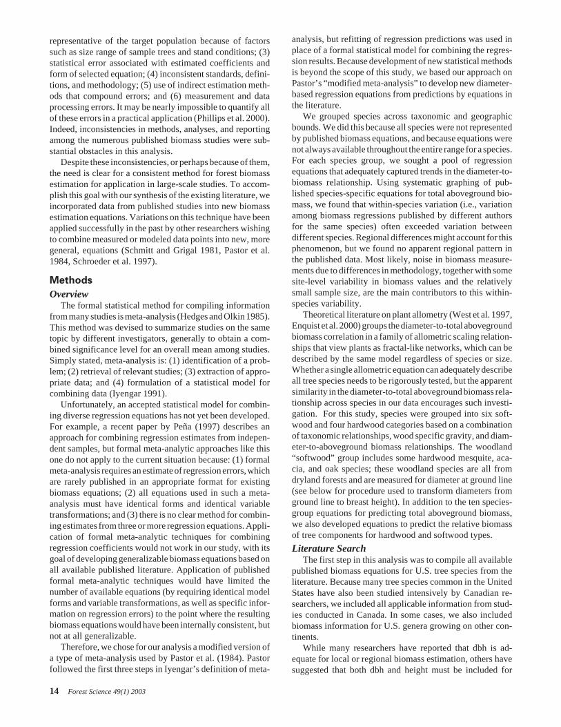
Table 1. Hardwood species groups for the diameter-based aboveground biomass equations.
Species groupNo. of
eqs. Genus SpeciesWood-specific
gravity* Literature reference †
Aspen/alder/ 36 Alnus rubra 0.37 7,8,44,55cottonwood/ sinuata 7willow spp. 0.37 71,83,101
Populus balsamifera 0.31 90deltoides 0.37 2,3,19,59grandidentata 0.36 32,54,100spp. 0.37 45,65,101tremuloides 0.35 16,32,47,51,58,61,72,74,76,78,83,85,90,96
Salix spp. 0.36 83,101Soft maple/ 47 Acer macrophyllum 0.44 33birch pensylvanicum 0.44 101
rubrum 0.49 12,22,23,25,26,32,45,51,53,61,63,65,77,81,83,100,101spicatum 0.44 14,60,79,101
Betula alleghaniensis 0.55 32,65,67,81,83,89,101lenta 0.60 15,45,63papyrifera 0.48 6,25,45,48,51,61,81,83,101populifolia 0.45 32,45,51,83,101
Mixed 40 Aesculus octandra 0.33 15hardwood Castanopsis chrysophylla 0.42 33
Cornus florida 0.64 10,63,77Fraxinus americana 0.55 65,100,101
nigra 0.45 71,81,101pennsylvanica 0.53 22
Liquidambar styraciflua 0.46 22,23,77Liriodendron tulipifera 0.40 15,22,23,63,77,100Nyssa aquatica 0.46 22
sylvatica 0.46 22,77,100Oxydendrum arboreum 0.50 63,77Platanus occidentalis 0.46 23Prunus pensylvanica 0.36 15,61,83,101
serotina 0.47 100virginiana 0.36 83,101
Sassafras albidum 0.42 100Tilia americana 0.32 45,101
heterophylla 0.32 15Ulmus americana 0.46 81
spp. 0.50 23Hard maple/ 49 Acer saccharum 0.56 15,20,25,32,45,65,67,72,83,89,100,101oak/hickory Carya spp. 0.62 22,23,63,77beech Fagus grandifolia 0.56 15,45,65,83,89,101
Quercus alba 0.60 22,23,63,77,81,98coccinea 0.60 23,63,98ellipsoidalis 0.56 81falcata 0.52 23,77laurifolia 0.56 22nigra 0.56 22prinus 0.57 23,63,77rubra 0.56 15,20,36,45,53,63,65,101stellata 0.60 23,77velutina 0.56 100
* US Forest Products Laboratory. 1974. Wood handbook: Wood as an engineering material. USDA Agric. Handb. 72, rev.† Reference numbers are matched to authors in Table 2. Reference number 32 for Freedman’s combined species equation is also included in
each species group.
Forest Science 49(1) 2003 17
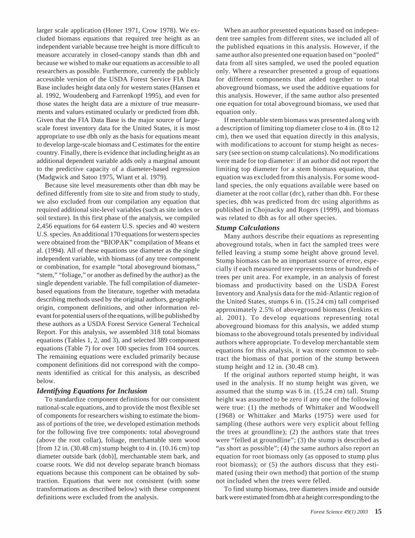
Table 2. Key to reference numbers in Tables 1 and 3.
Ref. no. Author reference Ref. no. Author reference1 Acker and Easter (1994) 52 Ker and van Raalte (1981)2 Anurag et al. (1989) 53 Kinerson and Bartholomew (1977)3 Bajrang et al. (1996) 54 Koerper and Richardson (1980)4 Barclay et al. (1986) 55 Koerper (1994)5 Barney et al. (1978) 56 Krumlik (1974)6 Baskerville (1965) 57 Landis (1975)7 Binkley (1983) 58 Lieffers and Campbell (1984)8 Binkley and Graham (1981) 59 Lodhiyal et al. (1995)9 Bockheim and Lee (1984) 60 Lovenstein and Berliner (1993)10 Boerner and Kost (1986) 61 MacLean and Wein (1976)11 Bormann (1990) 62 Marshall and Wang (1995)12 Briggs et al. (1989) 63 Martin et al. (1998)13 Brown (1978) 64 Miller et al. (1981)14 Bunyavejchewin and Kiratiprayoon (1989) 65 Monteith (1979)15 Busing et al. (1993) 66 Moore and Verspoor (1973)16 Campbell et al. (1985) 67 Morrison (1990)17 Carlyle and Malcolm (1986) 68 Naidu et al. (1998)18 Carpenter (1983) 69 Nelson and Switzer (1975)19 Carter and White (1971) 70 Ouellet (1983)20 Chapman and Gower (1991) 71 Parker and Schneider (1975)21 Chojnacky (1984) 72 Pastor and Bockheim (1981)22 Clark et al. (1985) 73 Pearson et al. (1984)23 Clark et al. (1986) 74 Perala and Alban (1982)24 Clary and Tiedemann (1987) 75 Perala and Alban (1994)25 Crow (1976) 76 Peterson et al. (1970)26 Crow (1983) 77 Phillips (1981)27 Darling (1967) 78 Pollard (1972)28 Dudley and Fownes (1992) 79 Rajeev (1998)29 Felker et al. (1982) 80 Ralston (1973)30 Feller (1992) 81 Reiners (1972)31 Freedman (1984) 82 Rencz and Auclair (1980)32 Freedman et al. (1982) 83 Ribe (1973)33 Gholz et al. (1979) 84 Ross and Walstad (1986)34 Gower et al. (1987) 85 Ruark and Bockheim (1988)35 Gower et al. (1992) 86 Sachs (1984)36 Gower et al. (1993) 87 Schnell (1976)37 Green and Grigal (1978) 88 Schubert et al. (1988)38 Grier et al. (1984) 89 Siccama et al. (1994)39 Grier et al. (1992) 90 Singh (1984)40 Grigal and Kernik (1984) 91 St. Clair (1993)41 Harding and Grigal (1985) 92 Swank and Schreuder (1974)42 Harmon (1994) 93 Teller (1988)43 Hegyi (1972) 94 Van Lear et al. (1984)44 Helgerson et al. (1988) 95 Vertanen et al. (1993)45 Hocker and Earley (1978) 96 Wang et al. (1995)46 Honer (1971) 97 Westman (1987)47 Johnston and Bartos (1977) 98 Whittaker and Woodwell (1968)48 Jokela et al. (1981) 99 Whittaker and Niering (1975)49 Jokela et al. (1986) 100 Williams and McClenahen (1984)50 Ker (1980a) 101 Young et al. (1980)51 Ker (1980b)
tionship, so that it could be fitted with simple linearregression rather than a more complicated nonlinear model.Finally, a new linear equation was fitted from thepseudodata. In this way, the new regression was a synthe-sis of the original published regressions.
We modified this approach slightly. In our analysis, if therange between the minimum and maximum diameters of theoriginal equations was wider than 25 cm, the diameter rangewas divided by 5 to obtain (to the nearest integer) the numberof diameter values included for that equation, spaced at 5 cmintervals. If the upper diameter limit for a given equation was
larger than 100 cm, we spaced the diameter values larger than100 cm at 10 cm intervals to moderate the influence of thethese few large-tree equations. The median number ofpseudodata points per equation was 8, but 10% of theequations spanned diameter ranges that exceeded 100 cm;these large-tree equations were all developed for softwoodspecies and represented between 20 and 50 pseudodatapredictions each.
Generalized regression for total aboveground biom-ass.—The pseudodata developed from the published equa-tions were used to predict the relationships between tree dbh
18 Forest Science 49(1) 2003
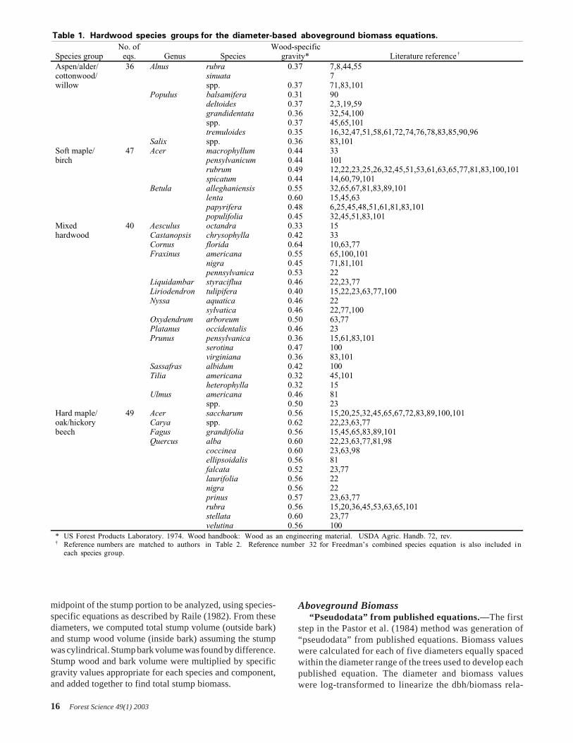
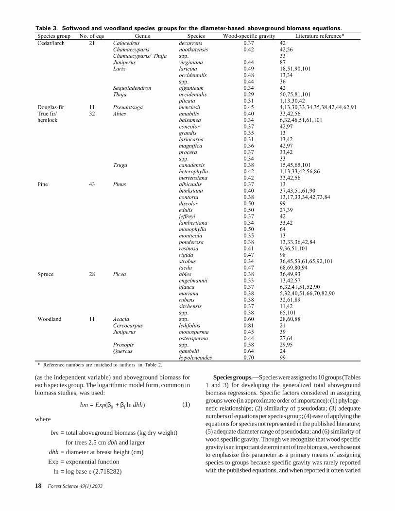
Table 3. Softwood and woodland species groups for the diameter-based aboveground biomass equations.
Species group No. of eqs Genus Species Wood-specific gravity Literature reference*Cedar/larch 21 Calocedrus decurrens 0.37 42
Chamaecyparis nootkatensis 0.42 42,56Chamaecyparis/ Thuja spp. 33Juniperus virginiana 0.44 87Larix laricina 0.49 18,51,90,101
occidentalis 0.48 13,34spp. 0.44 36
Sequoiadendron giganteum 0.34 42Thuja occidentalis 0.29 50,75,81,101
plicata 0.31 1,13,30,42Douglas-fir 11 Pseudotsuga menziesii 0.45 4,13,30,33,34,35,38,42,44,62,91True fir/ 32 Abies amabilis 0.40 33,42,56hemlock balsamea 0.34 6,32,46,51,61,101
concolor 0.37 42,97grandis 0.35 13lasiocarpa 0.31 13,42magnifica 0.36 42,97procera 0.37 33,42spp. 0.34 33
Tsuga canadensis 0.38 15,45,65,101heterophylla 0.42 1,13,33,42,56,86mertensiana 0.42 33,42,56
Pine 43 Pinus albicaulis 0.37 13banksiana 0.40 37,43,51,61,90contorta 0.38 13,17,33,34,42,73,84discolor 0.50 99edulis 0.50 27,39jeffreyi 0.37 42lambertiana 0.34 33,42monophylla 0.50 64monticola 0.35 13ponderosa 0.38 13,33,36,42,84resinosa 0.41 9,36,51,101rigida 0.47 98strobus 0.34 36,45,53,61,65,92,101taeda 0.47 68,69,80,94
Spruce 28 Picea abies 0.38 36,49,93engelmannii 0.33 13,42,57glauca 0.37 6,32,41,51,52,90mariana 0.38 5,32,40,51,66,70,82,90rubens 0.38 32,61,89sitchensis 0.37 11,42spp. 0.38 65,101
Woodland 11 Acacia spp. 0.60 28,60,88Cercocarpus ledifolius 0.81 21Juniperus monosperma 0.45 39
osteosperma 0.44 27,64Prosopis spp. 0.58 29,95Quercus gambelii 0.64 24
hypoleucoides 0.70 99* Reference numbers are matched to authors in Table 2.
(as the independent variable) and aboveground biomass foreach species group. The logarithmic model form, common inbiomass studies, was used:
bm Exp dbh= +( ln )β β0 1 (1)
where
bm
dbh
dbh
=
===
total aboveground biomass (kg dry weight)
for trees 2.5 cm and larger
diameter at breast height (cm)
Exp exponential function
ln log base e (2.718282)
Species groups.—Species were assigned to 10 groups (Tables1 and 3) for developing the generalized total abovegroundbiomass regressions. Specific factors considered in assigninggroups were (in approximate order of importance): (1) phyloge-netic relationships; (2) similarity of pseudodata; (3) adequatenumbers of equations per species group; (4) ease of applying theequations for species not represented in the published literature;(5) adequate diameter range of pseudodata; and (6) similarity ofwood specific gravity. Though we recognize that wood specificgravity is an important determinant of tree biomass, we chose notto emphasize this parameter as a primary means of assigningspecies to groups because specific gravity was rarely reportedwith the published equations, and when reported it often varied
Forest Science 49(1) 2003 19
among different portions of an individual tree. Instead, wegrouped species primarily according to similarities in tree mor-phology, which are reflected in taxonomic affiliations. Wherevery few equations existed for species in a particular taxonomicgroup, pseudodata were examined and species were assigned togroups with similar dbh/biomass relationships.
Large trees.—In addition to ensuring that the speciesgroup equations were developed from adequate numbers ofpseudodata, came from populations with reasonably similardbh/biomass relationships and were appropriate for use withspecies not represented by a biomass equation, we ensuredthat each of the equations will be applicable for the entire dbhrange of stems growing in the United States. Inclusion oflarge-tree equations for each group was especially criticalbecause logistic regression equations may not extrapolatewell beyond the range of data. Based on the full set ofEastwide and Westwide FIA data (Hansen et al. 1992,Woudenberg et al. 1995), the largest softwood and hardwoodtrees measured in the most recent inventory sample in theUnited States were 250 and 230 cm, respectively. Amplesoftwood pseudodata included trees as large as 250 cm dbh,such that we were able to include one equation with a dbhlimit close to 250 cm in each of the softwood species groups.
However, published hardwood equations have upper dbhlimits ranging only from 56 to 73 cm. To ensure that ourgeneralized hardwood equations would be applicable at di-ameters substantially larger than this, the generalized hard-wood equation published by Freedman (1984) was used topredict biomass values for diameters between 100 and 230cm for each hardwood species group. This equation’s statedupper limit is 31.3 cm, so we were concerned that it might biasbiomass estimates at large dbh values. We plotted the gener-alized Freedman (1984) hardwood equation together with thepseudodata from the softwood equations based on measureddata to 250 cm that were used to develop the generalizedregressions in this analysis. The Freedman (1984) equationmatched the large-tree softwood equations closely at allvalues of dbh, suggesting that this equation does not contrib-ute to substantial bias at large dbh values.
While this solution is clearly not ideal, we re-emphasizethat there are no published hardwood regression equationsavailable for use in this analysis that were developed usinghardwood trees as large as the largest trees in the inventorysample. Furthermore, we assert that: (1) it is important for ourequations to be applicable at the large dbh values observed innature; (2) equations developed without this correction werequite clearly biased upward at large diameters; (3) availablemensurational datasets (e.g., Baker 1971, Sollins and Ander-son 1971, Crow 1976, Briggs et al. 1989) do not include treesat diameters approaching 230 cm; and (4) the only otherapproach to estimate biomass for hardwood trees with verylarge diameters would have been to use pseudodata fromequations developed for softwoods.
Correction factors.—Logarithmic regressions are reportedto result in a slight downward bias when data are back-trans-formed to arithmetic units (Baskerville 1972, Beauchamp andOlson 1973, Sprugel 1983). To remedy this problem, it has beenproposed that the back-transformed results (from natural loga-
rithmic units) be multiplied by a correction factor (CF), definedas exp(MSE/2) (Sprugel 1983), where MSE refers to the meansquared error of a line fit by least-squares regression. BecauseMSE varies inversely with sample size, however, the CF alsovaries with sample size. This does not necessarily result in moreaccurate estimates, and the correction itself might be biased forsmall sample sizes (Flewelling and Pienaar 1981). To avoid thebias potentially introduced by using such CFs, we uncorrectedany equation coefficients that were presented by the originalauthors as having been corrected, and we did not use CFs whenthey were presented separately. In addition, though our regres-sions are presented in logarithmic form, we do not include CFsfor the reader to use after back-transformation. The root meansquared error (RMSE) for each regression is included in Table4, however, for the reader who wishes to calculate CF values.
Goodness-of-fit.—Because our generalized regressions wererefit from published equations without using a technique thatincluded a measure of the variability of the equations, it wasdifficult to calculate confidence intervals or other standardregression statistics to assess prediction error. However, weexamined regression residuals in terms of percentage of pre-dicted value. The residuals (pseudodata minus predicted value)from the generalized regressions were first expressed in terms of“percent of the predicted value,” and these percentage valueswere ranked. Table 5 lists the 10th and 90th percentiles of theresidual distribution (expressed as percent of predicted value)for each species group, which is an upper and lower bound for80% of the pseudodata. These results indicated that 80% of thepseudodata fell within about 20 to 35% of our generalizedregression equations.
Comparison with other datasets.—As stated above, thereis no available, representative, and complete set of treemensurational data against which to compare our generalizedbiomass equations at the national scale. As a test of our equa-tions, then, we compared our equations against other equationsthat were developed to be reasonably generalizable, and whichhave also been used to develop large-scale biomass estimates.While this comparison cannot determine unequivocally whetherany of these equations truly represent the conditions observed innature, it can point out areas of disagreement and suggest topicsfor further study.
We predicted biomass for dbh values between 5 and 80 cmusing our equations and equations for northeastern species,which have also been applied to the USDA Forest ServiceFIA dataset for large-scale biomass estimation, published bySchroeder et al. (1997) and Brown et al. (1999). For thiscomparison, our four hardwood species group equationswere compared with the general hardwood equation pub-lished by Schroeder et al. (1997); our spruce and true fir/hemlock equations were compared with the spruce/fir equa-tion published by Brown and Schroeder (1999); and our pineequation was compared directly with the equation for pinepublished by Brown and Schroeder (1999). Three of ourspecies groups—Douglas-fir, woodland, and cedar/larch—were excluded from this analysis because trees in thesegroups were not represented in the dataset used by Schroederet al. (1997) and Brown and Schroeder (1999) to developtheir equations.
20 Forest Science 49(1) 2003
Component BiomassWe could not determine if the species groups used for total
aboveground biomass were appropriate for grouping compo-nents because adequate numbers of equations were not avail-able to predict the biomass of each component in each of thespecies groups. Attempts to devise new species groupingsraised suspicions that dbh-based allometric relationships fortree components are much more complex than for totalaboveground biomass. As a result, equations were pooledinto hardwood and softwood groups for component biomassestimation.
Merchantable stem and bark were defined from a 12 in.(30.48 cm) stump height to a 4 in. (10.16 cm) top (dob).Foliage estimates exclude twigs and include the currentyear’s foliage and petioles plus any previous year’s foliagestill on the tree. Due to the scarcity of root biomass equations,we included all equations describing root biomass, regardless
of the author’s definition of roots. While some authors did notspecify a root definition, most equations limited roots to aminimum diameter ranging from 0.15 to 5 cm. Where anauthor specified that an equation referred to stump plus roots,the biomass of the stump portion was calculated as describedabove and then subtracted to find root biomass only.
Where allometric equations were available for each com-ponent of interest [coarse roots, merchantable stem (woodand bark computed separately), and foliage], biomass esti-mates of component biomass were made and expressed asproportions of aboveground total biomass. The logarithms ofthese proportions were modeled as functions of inversediameter so that the ratios reach an asymptote for large trees:
ratiodbh
= +
Exp β
β0
1(2)
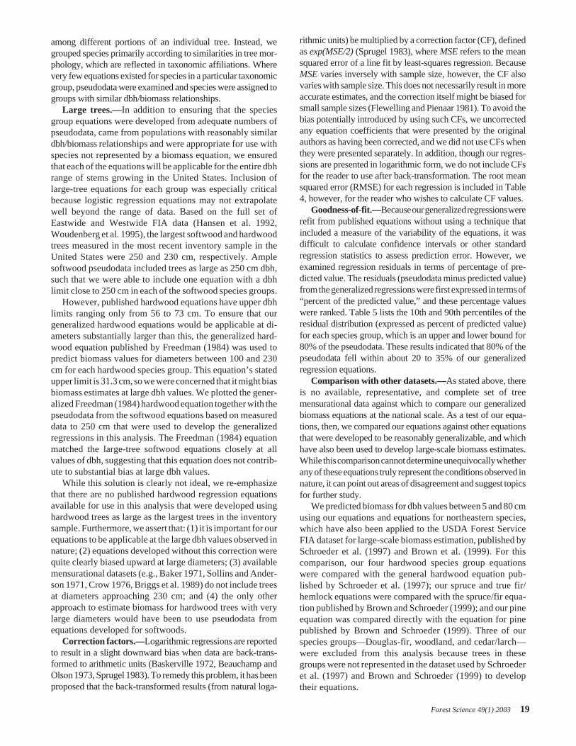
Table 4. Parameters and equations* for estimating total aboveground biomass for all hardwood and softwoodspecies in the United States.
ParametersSpecies group β0 β1
Datapoints†
Max ††dbhcm
RMSE §
log units R2
Hardwood Aspen/alder/cottonwood/willow –2.2094 2.3867 230 70 0.507441 0.953Soft maple/birch –1.9123 2.3651 316 66 0.491685 0.958Mixed hardwood –2.4800 2.4835 289 56 0.360458 0.980Hard maple/oak/hickory/beech –2.0127 2.4342 485 73 0.236483 0.988
Softwood Cedar/larch –2.0336 2.2592 196 250 0.294574 0.981Douglas-fir –2.2304 2.4435 165 210 0.218712 0.992True fir/hemlock –2.5384 2.4814 395 230 0.182329 0.992Pine –2.5356 2.4349 331 180 0.253781 0.987Spruce –2.0773 2.3323 212 250 0.250424 0.988
Woodland || Juniper/oak/mesquite –0.7152 1.7029 61 78 0.384331 0.938* Biomass equation:
bm dbh
bm
dbh
= +
====
Exp
where
total aboveground biomass (kg) for trees 2.5cm dbh and larger
diameter at breast height (cm)
Exp exponential function
ln natural log base "e" (2.718282)
( ln )β β0 1
† Number of data points generated from published equations (generally at 5 cm dbh intervals) for parameter estimation.†† Maximum dbh of trees measured in published equations.§ Root mean squared error or estimate of the standard deviation of the regression error term in natural log units.|| Woodland group includes both hardwood and softwood species from dryland forests.
Table 5. Distribution percentiles of regression residuals—expressed as a percentage of predicted value—foraboveground biomass equations (Table 4) for all hardwood and softwood species in United States.
Percent of predicted biomassSpecies group Data points* 10th percentile 90th percentile
Hardwood Aspen/alder/cottonwood/willow 230 –35.2 31.4Soft maple/birch 316 –23.8 28.5Mixed hardwood 289 –24.7 34.8Hard maple/oak/hickory/beech 485 –19.2 22.3
Softwood Cedar/larch 196 –33.7 35.7Douglas-fir 165 –23.0 27.2True fir/hemlock 395 –18.3 20.0Pine 331 –24.0 33.7Spruce 212 –24.4 28.7
Woodland † Juniper/oak/mesquite 61 –32.2 38.5* Number of data points generated from published equations (generally at 5 cm dbh intervals) for parameter estimation.† Woodland group includes both hardwood and softwood species from dryland forests.
Forest Science 49(1) 2003 21
where
ratio of component to total aboveground
biomass (dry weight) for trees
2.5 cm and larger
diameter at breast height (cm)
Exp exponential function
ln log base e (2.718282)
ratio
dbh
dbh
=
===
Due to the scarcity of component biomass equations and thesubstantial variation in component estimates, no attempt wasmade to quantify variability among published estimates.
Results and Discussion
Aboveground Biomass RegressionsAboveground biomass regression equations were devel-
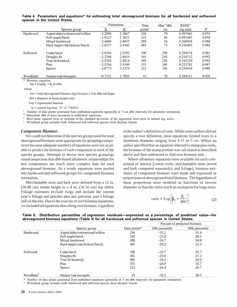
oped for four hardwood and six softwood species groups(Table 4). In general, the hardwood species had greaterbiomass at a given dbh than did the softwood species (Figure1). Two hardwood species groups—hard maple/oak/hickory/beech, and soft maple/birch—had the greatest biomass at agiven dbh. The woodland species had the lowest biomassvalues for a given diameter, and three of the softwood speciesgroups had the next-lowest biomass values: cedar/larch, pine,and spruce. The Douglas-fir species group had the largest ofthe softwood biomass values, while the aspen/alder/cotton-wood/willow group had the smallest of the hardwood biom-ass values.
Hardwood species groups.—The aspen/alder/cotton-wood/willow group, the lightest of the hardwood groups at agiven dbh, is comprised of species belonging to the Salicaceae
(Populus and Salix spp.) and Betulaceae (Alnus spp.) families.Though specific gravity was not used as the primary determi-nant of species grouping, these fast-growing species do havesimilar small bole wood specific gravity values (Table 1).Additional representatives of the Betulaceae family (Betulaspp.) occur in the soft maple/birch species group. Thesespecies were grouped with the soft maple species separatefrom the members of the Betulaceae family in the aspen/alder/cottonwood/willow group. The pseudodata developedfrom published equations for Betula species indicated thatthey were heavier at a given dbh than the Alnus species, andthat they were more similar to the soft maple species than tothe other members of their taxonomic group.
Sugar maple (Acer saccharum) was grouped with the hardmaple/oak/hickory/beech group, apart from the other mem-bers of its family Aceraceae. This split reflects the differentdbh/biomass relationships in the soft and hard maple species,as well as the higher bole wood specific gravity in sugarmaple compared to other species in the Aceraceae family.Species in the family Fagaceae, including oak (Quercus spp.)and American beech (Fagus grandifolia), had pseudodatathat matched sugar maple closely and were thus included inthis group, as were members of the Juglandaceae family(Carya spp.).
Forty equations were included in the mixed hardwoodgroup, compared with 36 in aspen/alder/cottonwood, 47 insoft maple/birch, and 49 in the hard maple/oak/hickory/beechgroup. However, more species and families are represented inthe mixed hardwood group—21 and 14, compared with 8species and 2 families in both the aspen/alder/cottonwood/willow and soft maple/birch groups, and 13 species in 3 familiesin the hard maple/oak/beech/hickory group. Because thepseudodata for different species and families, especially thespecies of intermediate bole wood specific gravity found in themixed hardwood group, often overlapped with one another, wegrouped the mixed hardwoods together unless it was clear thatthey belonged in one of the other three groups. This groupingwas consistent with the pseudodata distribution, resulted inreasonable prediction intervals about each of the groups, andallowed for more systematic group assignment of species notrepresented in the published literature.
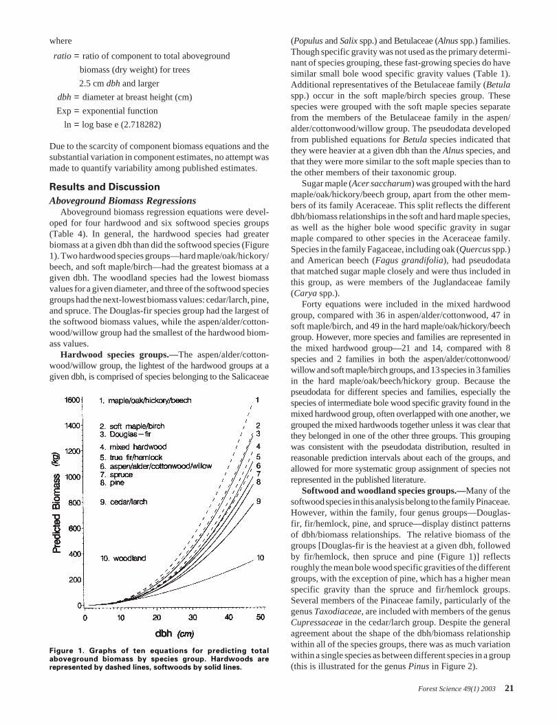
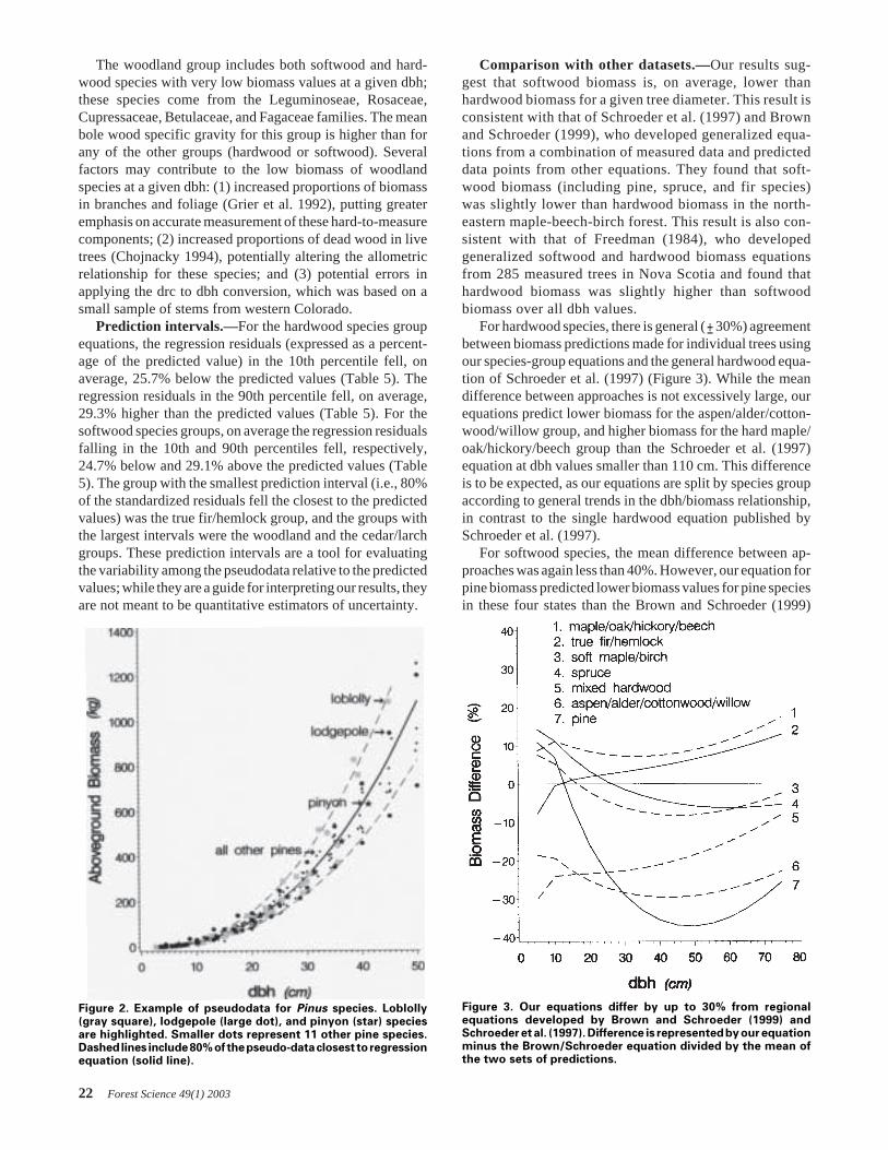
Softwood and woodland species groups.—Many of thesoftwood species in this analysis belong to the family Pinaceae.However, within the family, four genus groups—Douglas-fir, fir/hemlock, pine, and spruce—display distinct patternsof dbh/biomass relationships. The relative biomass of thegroups [Douglas-fir is the heaviest at a given dbh, followedby fir/hemlock, then spruce and pine (Figure 1)] reflectsroughly the mean bole wood specific gravities of the differentgroups, with the exception of pine, which has a higher meanspecific gravity than the spruce and fir/hemlock groups.Several members of the Pinaceae family, particularly of thegenus Taxodiaceae, are included with members of the genusCupressaceae in the cedar/larch group. Despite the generalagreement about the shape of the dbh/biomass relationshipwithin all of the species groups, there was as much variationwithin a single species as between different species in a group(this is illustrated for the genus Pinus in Figure 2).
Figure 1. Graphs of ten equations for predicting totalaboveground biomass by species group. Hardwoods arerepresented by dashed lines, softwoods by solid lines.
22 Forest Science 49(1) 2003
The woodland group includes both softwood and hard-wood species with very low biomass values at a given dbh;these species come from the Leguminoseae, Rosaceae,Cupressaceae, Betulaceae, and Fagaceae families. The meanbole wood specific gravity for this group is higher than forany of the other groups (hardwood or softwood). Severalfactors may contribute to the low biomass of woodlandspecies at a given dbh: (1) increased proportions of biomassin branches and foliage (Grier et al. 1992), putting greateremphasis on accurate measurement of these hard-to-measurecomponents; (2) increased proportions of dead wood in livetrees (Chojnacky 1994), potentially altering the allometricrelationship for these species; and (3) potential errors inapplying the drc to dbh conversion, which was based on asmall sample of stems from western Colorado.
Prediction intervals.—For the hardwood species groupequations, the regression residuals (expressed as a percent-age of the predicted value) in the 10th percentile fell, onaverage, 25.7% below the predicted values (Table 5). Theregression residuals in the 90th percentile fell, on average,29.3% higher than the predicted values (Table 5). For thesoftwood species groups, on average the regression residualsfalling in the 10th and 90th percentiles fell, respectively,24.7% below and 29.1% above the predicted values (Table5). The group with the smallest prediction interval (i.e., 80%of the standardized residuals fell the closest to the predictedvalues) was the true fir/hemlock group, and the groups withthe largest intervals were the woodland and the cedar/larchgroups. These prediction intervals are a tool for evaluatingthe variability among the pseudodata relative to the predictedvalues; while they are a guide for interpreting our results, theyare not meant to be quantitative estimators of uncertainty.
Comparison with other datasets.—Our results sug-gest that softwood biomass is, on average, lower thanhardwood biomass for a given tree diameter. This result isconsistent with that of Schroeder et al. (1997) and Brownand Schroeder (1999), who developed generalized equa-tions from a combination of measured data and predicteddata points from other equations. They found that soft-wood biomass (including pine, spruce, and fir species)was slightly lower than hardwood biomass in the north-eastern maple-beech-birch forest. This result is also con-sistent with that of Freedman (1984), who developedgeneralized softwood and hardwood biomass equationsfrom 285 measured trees in Nova Scotia and found thathardwood biomass was slightly higher than softwoodbiomass over all dbh values.
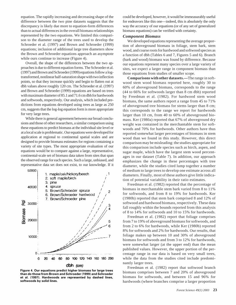
For hardwood species, there is general (± 30%) agreementbetween biomass predictions made for individual trees usingour species-group equations and the general hardwood equa-tion of Schroeder et al. (1997) (Figure 3). While the meandifference between approaches is not excessively large, ourequations predict lower biomass for the aspen/alder/cotton-wood/willow group, and higher biomass for the hard maple/oak/hickory/beech group than the Schroeder et al. (1997)equation at dbh values smaller than 110 cm. This differenceis to be expected, as our equations are split by species groupaccording to general trends in the dbh/biomass relationship,in contrast to the single hardwood equation published bySchroeder et al. (1997).
For softwood species, the mean difference between ap-proaches was again less than 40%. However, our equation forpine biomass predicted lower biomass values for pine speciesin these four states than the Brown and Schroeder (1999)
Figure 3. Our equations differ by up to 30% from regionalequations developed by Brown and Schroeder (1999) andSchroeder et al. (1997). Difference is represented by our equationminus the Brown/Schroeder equation divided by the mean ofthe two sets of predictions.
Figure 2. Example of pseudodata for Pinus species. Loblolly(gray square), lodgepole (large dot), and pinyon (star) speciesare highlighted. Smaller dots represent 11 other pine species.Dashed lines include 80% of the pseudo-data closest to regressionequation (solid line).
Forest Science 49(1) 2003 23
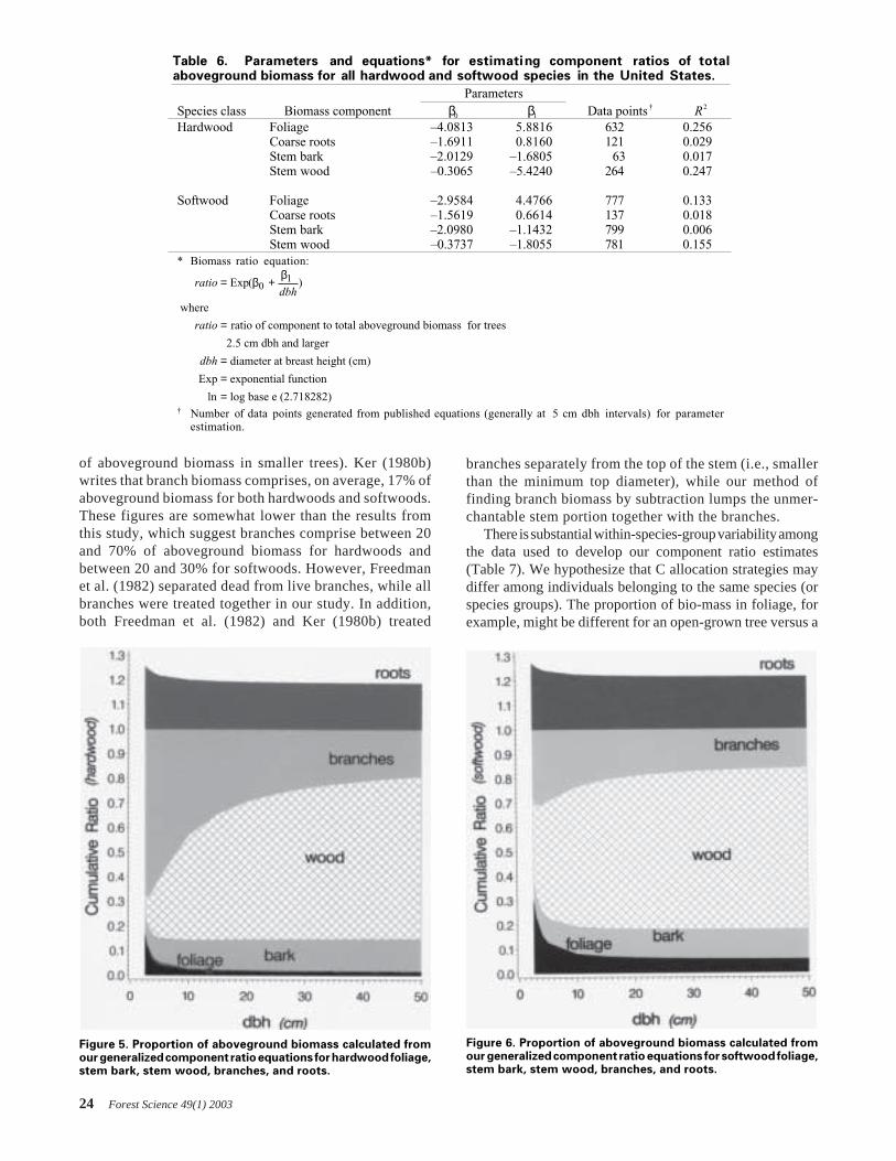
equation. The rapidly increasing and decreasing shape of thedifference between the two pine datasets suggests that thediscrepancy is likely due more to equation-form differencesthan to actual differences in the overall biomass relationshipsrepresented by the two equations. We limited this compari-son to the diameter range of the trees used to develop theSchroeder et al. (1997) and Brown and Schroeder (1999)equations; inclusion of additional large tree diameters showthe Brown and Schroeder equations approach an asymptotewhile ours continue to increase (Figure 4).
Overall, the shape of the differences between the two ap-proaches is due to different equation forms. The Schroeder et al.(1997) and Brown and Schroeder (1999) equations follow a log-transformed, nonlinear half-saturation shape with two inflectionpoints, so that they increase quickly and begin to flatten out atdbh values above roughly 120 cm. The Schroeder et al. (1997)and Brown and Schroeder (1999) equations are based on treeswith maximum diameter of 85.1 and 71.6 cm dbh for hardwoodsand softwoods, respectively. Our analysis, which included pre-dictions from equations developed using trees as large as 250cm, suggests that the log-log equation form is more appropriatefor very large trees.
While there is general agreement between our broad conclu-sions and those of other researchers, a similar comparison usingthese equations to predict biomass at the individual site level orat a local scale is problematic. Our equations were developed forapplication at regional to continental spatial scales and aredesigned to provide biomass estimates for regions containing avariety of site types. The most appropriate evaluation of ourequations would be to compare against a large, representative,continental-scale set of biomass data taken from sites that spanthe observed range for each species. Such a large, unbiased, andrepresentative data set does not exist, to our knowledge. If it
could be developed, however, it would be immeasurably usefulfor endeavors like this one—indeed, this is absolutely the onlyway the accuracy of our equations (or of any set of generalizedbiomass equations) can be verified with certainty.
Component BiomassWe developed equations representing the average propor-
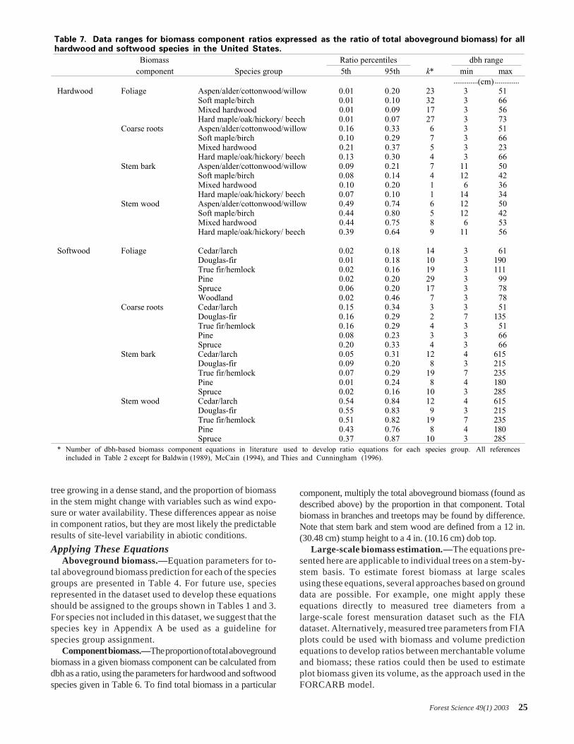
tion of aboveground biomass in foliage, stem bark, stemwood, and coarse roots for hardwood and softwood species asa function of dbh (Tables 6 and 7, Figures 5 and 6). Branch(bark and wood) biomass was found by difference. Becauseour equations represent many species over a large variety ofsites, we expect a larger range in component biomass thanthose equations from studies of smaller scope.
Comparisons with other datasets.—The range in soft-wood stem wood biomass reported here, roughly 30 to60% of aboveground biomass, corresponds to the range(44 to 66% for softwoods larger than 8 cm dbh) reportedby Freedman et al. (1982). For hardwood stem woodbiomass, the same authors report a range from 45 to 71%of aboveground tree biomass for stems larger than 8 cm;this corresponds to the range we report for hardwoodslarger than 10 cm, from 40 to 60% of aboveground bio-mass. Ker (1980a) reported that 67% of aboveground dryweight was contained in the merchantable stem for soft-woods and 70% for hardwoods. Other authors have thusreported somewhat larger percentages of biomass in stemwood than we found in this study. However, this directcomparison may be misleading: the studies appropriate forthis comparison include species such as birch, aspen, andsugar maple, which have the largest stem wood percent-ages in our dataset (Table 7). In addition, our approachemphasizes the change in these percentages with treediameter, while the studies cited lump together a numberof medium to large trees to develop one estimate across alldiameters. Finally, most of these authors give little indica-tion of potential variability in their ratio estimates.
Freedman et al. (1982) reported that the percentage ofbiomass in merchantable stem bark varied from 8 to 11%for softwoods, and from 8 to 19% for hardwoods. Ker(1980b) reported that stem bark comprised 8 and 12% ofsoftwood and hardwood biomass, respectively. These datafall roughly within the bounds reported from this analysisof 8 to 14% for softwoods and 10 to 15% for hardwoods.
Freedman et al. (1982) report that foliage comprisesfrom 7 to 19% of aboveground biomass for softwoods, andfrom 2 to 6% for hardwoods, while Ker (1980b) reported8% for softwoods and 2% for hardwoods. Our results, thatfoliage makes up between 10 and 30% of abovegroundbiomass for softwoods and from 3 to 12% for hardwoods,were somewhat larger (at the upper end) than the meanpublished values. However, the upper portion of the per-centage range in our data is based on very small trees,while the data from the studies cited include predomi-nantly larger trees.
Freedman et al. (1982) report that softwood branchbiomass comprises between 7 and 20% of abovegroundbiomass for softwoods, and between 15 and 96% forhardwoods (where branches comprise a larger proportion
Figure 4. Our equations predict higher biomass for large treesthan do those from Brown and Schroeder (1999) and Schroederet al. (1997). Hardwoods are represented by dashed lines,softwoods by solid lines.
24 Forest Science 49(1) 2003
Table 6. Parameters and equations* for estimating component ratios of totalaboveground biomass for all hardwood and softwood species in the United States.
ParametersSpecies class Biomass component β0 β1 Data points † R2
Hardwood Foliage –4.0813 5.8816 632 0.256Coarse roots –1.6911 0.8160 121 0.029Stem bark –2.0129 –1.6805 63 0.017Stem wood –0.3065 –5.4240 264 0.247
Softwood Foliage –2.9584 4.4766 777 0.133Coarse roots –1.5619 0.6614 137 0.018Stem bark –2.0980 –1.1432 799 0.006Stem wood –0.3737 –1.8055 781 0.155
* Biomass ratio equation:
ratio
ratio
= +
=
===
Exp
where
ratio of component to total aboveground biomass for trees
2.5 cm dbh and larger
diameter at breast height (cm)
Exp exponential function
ln log base e (2.718282)
( )ββ
01
dbh
dbh
† Number of data points generated from published equations (generally at 5 cm dbh intervals) for parameterestimation.
of aboveground biomass in smaller trees). Ker (1980b)writes that branch biomass comprises, on average, 17% ofaboveground biomass for both hardwoods and softwoods.These figures are somewhat lower than the results fromthis study, which suggest branches comprise between 20and 70% of aboveground biomass for hardwoods andbetween 20 and 30% for softwoods. However, Freedmanet al. (1982) separated dead from live branches, while allbranches were treated together in our study. In addition,both Freedman et al. (1982) and Ker (1980b) treated
branches separately from the top of the stem (i.e., smallerthan the minimum top diameter), while our method offinding branch biomass by subtraction lumps the unmer-chantable stem portion together with the branches.
There is substantial within-species-group variability amongthe data used to develop our component ratio estimates(Table 7). We hypothesize that C allocation strategies maydiffer among individuals belonging to the same species (orspecies groups). The proportion of bio-mass in foliage, forexample, might be different for an open-grown tree versus a
Figure 5. Proportion of aboveground biomass calculated fromour generalized component ratio equations for hardwood foliage,stem bark, stem wood, branches, and roots.
Figure 6. Proportion of aboveground biomass calculated fromour generalized component ratio equations for softwood foliage,stem bark, stem wood, branches, and roots.
Forest Science 49(1) 2003 25
Table 7. Data ranges for biomass component ratios expressed as the ratio of total aboveground biomass) for allhardwood and softwood species in the United States.
Biomass Ratio percentiles dbh rangecomponent Species group 5th 95th k* min max
.............(cm) .............Hardwood Foliage Aspen/alder/cottonwood/willow 0.01 0.20 23 3 51
Soft maple/birch 0.01 0.10 32 3 66Mixed hardwood 0.01 0.09 17 3 56Hard maple/oak/hickory/ beech 0.01 0.07 27 3 73
Coarse roots Aspen/alder/cottonwood/willow 0.16 0.33 6 3 51Soft maple/birch 0.10 0.29 7 3 66Mixed hardwood 0.21 0.37 5 3 23Hard maple/oak/hickory/ beech 0.13 0.30 4 3 66
Stem bark Aspen/alder/cottonwood/willow 0.09 0.21 7 11 50Soft maple/birch 0.08 0.14 4 12 42Mixed hardwood 0.10 0.20 1 6 36Hard maple/oak/hickory/ beech 0.07 0.10 1 14 34
Stem wood Aspen/alder/cottonwood/willow 0.49 0.74 6 12 50Soft maple/birch 0.44 0.80 5 12 42Mixed hardwood 0.44 0.75 8 6 53Hard maple/oak/hickory/ beech 0.39 0.64 9 11 56
Softwood Foliage Cedar/larch 0.02 0.18 14 3 61Douglas-fir 0.01 0.18 10 3 190True fir/hemlock 0.02 0.16 19 3 111Pine 0.02 0.20 29 3 99Spruce 0.06 0.20 17 3 78Woodland 0.02 0.46 7 3 78
Coarse roots Cedar/larch 0.15 0.34 3 3 51Douglas-fir 0.16 0.29 2 7 135True fir/hemlock 0.16 0.29 4 3 51Pine 0.08 0.23 3 3 66Spruce 0.20 0.33 4 3 66
Stem bark Cedar/larch 0.05 0.31 12 4 615Douglas-fir 0.09 0.20 8 3 215True fir/hemlock 0.07 0.29 19 7 235Pine 0.01 0.24 8 4 180Spruce 0.02 0.16 10 3 285
Stem wood Cedar/larch 0.54 0.84 12 4 615Douglas-fir 0.55 0.83 9 3 215True fir/hemlock 0.51 0.82 19 7 235Pine 0.43 0.76 8 4 180Spruce 0.37 0.87 10 3 285
* Number of dbh-based biomass component equations in literature used to develop ratio equations for each species group. All referencesincluded in Table 2 except for Baldwin (1989), McCain (1994), and Thies and Cunningham (1996).
tree growing in a dense stand, and the proportion of biomassin the stem might change with variables such as wind expo-sure or water availability. These differences appear as noisein component ratios, but they are most likely the predictableresults of site-level variability in abiotic conditions.
Applying These EquationsAboveground biomass.—Equation parameters for to-
tal aboveground biomass prediction for each of the speciesgroups are presented in Table 4. For future use, speciesrepresented in the dataset used to develop these equationsshould be assigned to the groups shown in Tables 1 and 3.For species not included in this dataset, we suggest that thespecies key in Appendix A be used as a guideline forspecies group assignment.
Component biomass.—The proportion of total abovegroundbiomass in a given biomass component can be calculated fromdbh as a ratio, using the parameters for hardwood and softwoodspecies given in Table 6. To find total biomass in a particular
component, multiply the total aboveground biomass (found asdescribed above) by the proportion in that component. Totalbiomass in branches and treetops may be found by difference.Note that stem bark and stem wood are defined from a 12 in.(30.48 cm) stump height to a 4 in. (10.16 cm) dob top.
Large-scale biomass estimation.—The equations pre-sented here are applicable to individual trees on a stem-by-stem basis. To estimate forest biomass at large scalesusing these equations, several approaches based on grounddata are possible. For example, one might apply theseequations directly to measured tree diameters from alarge-scale forest mensuration dataset such as the FIAdataset. Alternatively, measured tree parameters from FIAplots could be used with biomass and volume predictionequations to develop ratios between merchantable volumeand biomass; these ratios could then be used to estimateplot biomass given its volume, as the approach used in theFORCARB model.
26 Forest Science 49(1) 2003
Table 8. Potential sources of error in allometric biomass estimation at large scales using species- and region-specific equations versus the generalized equations developed in this study.
Type of application Potential source of errorSpecies- and site-specific equations
applied to national scale(a) Coefficients developed for one species (or species group) may not apply to another species
(or species group).(b) Coefficients developed for one site may not apply to another site.(c) Sample trees and wood density samples may not be representative of the target population
because of factors such as size range of sample trees and stand conditions.(d) Relationship of trees used to develop specific regression to the target population (i.e., all
trees) is unknown.(e) Statistical error may be associated with estimated coefficients and form of selected equation.(f) Inconsistent standards, definitions, and methodology.(g) Use of indirect estimation methods may compound errors.(h) Measurement and data processing errors.(i) Regional boundaries may be sharply delineated due to differences in methodology.
(a) Generalized equations may be biased in favor of species for which published equations exist.Generalized equations (this study)applied to national scale (b) Relationship of trees used to develop generalized regression to the target population (i.e. all
trees) is unknown.(c) Potential bias in applying generalized equations to species where no published equations
exist.(d) No obvious way to estimate uncertainty or variability.(e) Generalized equations may inherit shortcomings of published equations, including:
(i) statistical error associated with estimated coefficients and form of selected equation,(ii) inconsistent standards, definitions, and methodology,(iii) use of indirect estimation methods that compound errors, and(iv) measurement and data processing errors.
There is potential error in using these equations. Forclarity, we provide a summary of the potential errorsinherent in using two different methods for large-scalebiomass estimation (Table 8). For this purpose, we havecompared errors potentially introduced in using individualspecies- and site-specific equations as they currently existin the literature with the errors potentially introduced byusing the generalized regression equations presented here.We emphasize, however, that: (1) errors are potentiallyintroduced whenever an allometric method is used toestimate biomass, no matter what method and at whatspatial scale; (2) it may not be feasible to ascertain whetherany of these errors is actually introduced; and (3) ourgeneralized equations represent the most comprehensiveeffort to date to develop consistent, accurate biomassequations for application all across the United States.
Conclusions
In this analysis, we performed a thorough review ofavailable biomass literature and a rigorous analysis of asubset of pseudodata derived from that literature. We foundthat many of the published equations were unusable for large-scale application because of inconsistencies in methodologyand definitions, incomplete reporting of methods, lack ofaccess to original data, and sampling from narrow segmentsof the population of trees of the United States. Our equationsmay be applied for large-scale analyses of biomass or carbonstocks and trends, but should be used cautiously at very smallscales where local equations may be more appropriate.
The clear variability in tree C allocation from site to siteand from study to study suggests that more information isneeded about the differences in biomass and allocationamong different tree species and sites. This variability
makes it difficult to estimate tree biomass accurately evenwhen a site-specific regression equation is used. Develop-ment of continental-scale regressions of known accuracyrequires a continental-scale measurement campaign, inwhich individuals of all species and sizes are measured,over the entire range of site conditions typical of eachspecies. This would be a formidable task.
In future work, we strongly suggest that a consistent set ofmeasurement and reporting protocols be adopted for biomassmeasurement studies (Clark 1979, Crow 1983) and thatresearchers publish the raw data from which their regressionswere developed in addition to the equations themselves. Thiswould facilitate future efforts to synthesize the biomassliterature. We suggest that an effort be made to sample treesacross the entire diameter range of a species, as well; anyanalysis of available biomass equations suffers from the clearlack of biomass equations for predicting biomass (especiallyfor hardwoods) at large diameters.
Literature CitedACKER, S., AND M. EASTER. 1994. Unpublished equations. In Software for
computing plant biomass—BIOPAK Users Guide, Means, J., et al.(eds.). USDA For. Serv. Gen. Tech. Rep. PNW-GTR-340.
ANURAG, R., M. SRIVASTAVA, AND A. RAIZADA. 1989. Biomass yield andbiomass equations for Populus deltoides Marsh. Indian J. For.12:56–61.
BAJRANG, S., P. MISRA, AND B. SINGH. 1996. Biomass, energy content andfuel-wood properties of Populus deltoides clones raised in North Indianplains. Indian J. For. 18:278–284.
BAKER, J. 1971. Response of sapling loblolly pine (Pinus taeda L.) tonitrogen fertilization: Growth, accumulation, and recovery. Ph.D. thesis,Mississippi State University, Mississippi State, MS.
BALDWIN, V.J. 1989. Is sapwood area a better predictor of loblolly pinecrown biomass than bole diameter? Biomass 20:177–185.
Forest Science 49(1) 2003 27
BARCLAY, H., P. PANG, AND D. POLLARD. 1986. Aboveground biomassdistribution within trees and stands in thinned and fertilized Douglas-fir. Can. J. For. Res. 16:438–442.
BARNEY, R.J., K. VAN CLEVE, and SCHLENTNER. 1978. Biomass distributionand crown characteristics in two Alaskan Picea mariana ecosystems.Can. J. For. Res. 8:36–41.
BASKERVILLE, G. 1965. Dry-matter production in immature balsam firstands. For. Sci. Monogr. 9.
BASKERVILLE, G.L. 1972. Use of logarithmic regression in the estimation ofplant biomass. Can. J. For. Res. 2:49–53.
BEAUCHAMP, J.J., AND J.S. OLSON. 1973. Corrections for bias in regressionestimates after logarithmic transformation. Ecology 54:1403–1407.
BINKLEY, D., AND R. GRAHAM. 1981. Biomass, production, and nutrientcycling of mosses in an old-growth Douglas-fir forest. Ecology62:1387–1389.
BINKLEY, D. 1983. Ecosystem production in Douglas-fir plantations:Interaction of red alder and site fertility. For. Ecol. Manage. 5:215–227.
BIRDSEY, R.A., AND H.T. SCHREUDER. 1992. An overview of forest inventoryand analysis estimation procedures in the Eastern United States—withan emphasis on the components of change. USDA For. Serv. Gen. Tech.Rep. RM-GTR-214.
BIRDSEY, R.A., AND L.S. HEATH. 1995. Carbon changes in U.S. forests. P.56–70, in Productivity of America’s forests and climate change, Joyce,L.A. (ed.). USDA For. Serv. Gen. Tech. Rep. RM-GTR-271.
BOCKHEIM, J., AND S. LEE. 1984. Biomass and net primary productionequations for thinned red pine plantations in central Wisconsin. Univ.of Wisconsin Coll. of Agric. For. Res. Notes No. 256.
BOERNER, R., AND J. KOST. 1986. Biomass equations for flowering dogwood,Cornus florida L. Castanea 51:153–155.
BORMANN, B. 1990. Diameter-based biomass regression models ignorelarge sapwood-related variation in Sitka spruce. Can. J. For. Res.20:1098–1104.
BRIGGS, R., J. PORTER, AND E. WHITE. 1989. Component biomass equationsfor Acer rubrum and Fagus grandifolia. State Univ. of New York Coll.of Environ. Sci. and For., Fac. of For. Tech. Publ. No. 4.
BROWN, J. 1978. Weight and density of crowns of Rocky Mountain conifers.USDA For. Serv. Res. Pap. INT–197.
BROWN, S.L., P. SCHROEDER, AND J.S. KERN. 1999. Spatial distribution ofbiomass in forests of the Eastern USA. For. Ecol. Manage. 123:81–90.
BUNYAVEJCHEWIN, S., AND S. KIRATIPRAYOON. 1989. Primary production ofplots of five young close–spaced fast-growing tree species I. Biomassequations. Natur. Hist. Bull. Siam Soc, 37:47–56.
BUSING, R., E. CLEBSCH, AND P. WHITE. 1993. Biomass and production ofsouthern Appalachian cove forests reexamined. Can. J. For. Res.23:760–765.
CAMPBELL, J.S., V.J. LIEFFERS, AND E.C. PIELOU. 1985. Regressionequations for estimating single tree biomass of trembling aspen:Assessing their applicability to more than one population. For. Ecol.Manage. 11:283–295.
CARLYLE, J., AND D. MALCOLM. 1986. Biomass and element capital of a 7-year-old lodgepole pine (Pinus contorta Dougl.) stand growing on deeppeat. For. Ecol. Manage. 14:285–291.
CARPENTER, E. 1983. Above-ground weights for tamarack in northeasternMinnesota. USDA For. Serv. Res. Pap. NC-245.
CARTER, M., AND E. WHITE. 1971. Dry weight and nutrient accumulation inyoung stands of cottonwood (Populus deltoides Bartr.). Auburn Univ.Agric. Exp. Sta. Circ. 190.
CHAPMAN, J., AND S. GOWER. 1991. Aboveground production and canopydynamics in sugar maple and red oak trees in southwestern Wisconsin.Can. J. For. Res. 21:1533–1543.
CHOJNACKY, D. 1984. Volume and biomass for curlleaf cercocarpus inNevada. USDA For. Serv. Res. Pap. INT-332.
CHOJNACKY, D. 1994. Volume equations for New Mexico’s pinyon-juniperdryland forests. USDA For. Serv. Res. Pap. INT-471.
CHOJNACKY, D.C., AND P. ROGERS. 1999. Converting tree diameter measuredat root collar to diameter at breast height. West. J. Appl. For. 14:14–16.
CLARK, A.I. 1979. Suggested procedures for measuring tree biomass andreporting tree prediction equations. P. 615–628 in Forest resourceinventories. Vol. 2. Frayer, W. (ed.). Colorado State Univ., FortCollins, CO.
CLARK, A.I., AND J. SCHROEDER. 1986. Weight, volume, and physical propertiesof major hardwood species in the southern Appalachian mountains.USDA For. Serv. Res. Pap. SE-153.
CLARK, A.I., D. PHILLIPS, AND D. FREDERICK. 1985. Weight, volume, andphysical properties of major hardwood species in the Gulf and AtlanticCoastal Plains. USDA For. Serv. Res. Pap. SE-250.
CLARK, A.I., D. PHILLIPS, AND D. FREDERICK. 1986a. Weight, volume, andphysical properties of major hardwood species in the Piedmont. USDAFor. Serv. Res. Pap. SE-255.
CLARK, A.I., D. PHILLIPS, AND D. FREDERICK. 1986b. Weight, volume, andphysical properties of major hardwood species in the upland south.USDA For. Serv. Res. Pap. SE-257.
CLARY, W., AND A. TIEDEMANN. 1987. Fuelwood potential in large-treeQuercus gambelii stands. West. J. Appl. For. 2:87–90.
CROW, T.R. 1976. Biomass and production regressions for trees and woodyshrubs common to the Enterprise Forest. P. 63–67 in The Enterpriseradiation forest: Radioecological studies, Zavitkovski, J. (ed.). USEnergy Res. Dev. Adm. Rep. TID-26113-P2.
CROW, T.R. 1978. Biomass and production in three contiguous forests innorthern Wisconsin. Ecology 59:265–273.
CROW, T.R. 1983. Comparing biomass regressions by site and stand age forred maple. Can. J. For. Res. 13:283–288.
DARLING, M.L. 1967. Structure and productivity of pinyon-juniper woodlandin northern Arizona. Ph.D. Diss., Duke University, Durham, NC.
DUDLEY, N., AND J. FOWNES. 1992. Preliminary biomass equations for eightspecies of fast-growing tropical trees. J. Trop. For. Sci. 5:68–73.
ENQUIST, B., G. WEST, and J. BROWN. 2000. Quarter-power allometricscaling in vascular plants: functional basis and ecological consequences.P. 167–199 in Scaling in biology, Brown, J., and G. West (eds.). OxfordUniversity Press, Oxford.
FELKER, P., P. CLARK, J. OSBORN, and G. CANNELL. 1982. Biomass estimationin a young stand of mesquite (Prosopis spp.), ironwood (Olneya tesota),palo verde (Cercidium floridium and Parkinsonia aculeata), and leucaena(Leucaena leucocephala). J. Range Manage. 35(1):87–89.
FELLER, M. 1992. Generalized versus site-specific biomass regressionequations for Pseudotsuga menziesii var. menziesii and Thuja plicata incoastal British Columbia. Bioresource Tech. 39:9–16.
FLEWELLING, J.W., AND L.V. PIENAAR. 1981. Multiplicative regression withlognormal errors. For. Sci. 27:281–289.
FREEDMAN, B. 1984. The relationship between the aboveground dry weightand diameter for a wide size range of erect land plants. Can. J. Bot.62:2370–2374.
FREEDMAN, B., P. DUINKER, H. BARCLAY, R. MORASH, AND U. PRAGER. 1982.Forest biomass and nutrient studies in central Nova Scotia. MaritimesForest Research Centre, Can. For. Serv., Dep. of the Environ. Inf. Rep.M-X-134.
GHOLZ, H.L., C.C. GRIER, A.G. CAMPBELL, AND A.T. BROWN. 1979. Equationsfor estimating biomass and leaf area of plants in the Pacific Northwest.Oregon State Univ. School of For. For. Res. Lab Res. Pap. No. 41.
GOWER, S., C. GRIER, D. VOGT, AND K. VOGT. 1987. Allometric relations ofdeciduous (Larix occidentalis) and evergreen conifers (Pinus contortaand Pseudotsuga menziesii) of the Cascade Mountains in centralWashington. Can. J. For. Res. 17:630–634.
28 Forest Science 49(1) 2003
GOWER, S.T., K.A. VOGT, AND C.C. GRIER. 1992. Carbon dynamics ofRocky Mountain douglas-fir: Influence of water and nutrientavailability. Ecol. Monogr. 62:43–65.
GOWER, S.T., P.B. REICH, AND Y. SON. 1993. Canopy dynamics andaboveground production of five tree species with different leaflongevities. Tree Physiol. 12:327–345.
GREEN, D., AND D. GRIGAL. 1978. Generalized biomass estimationequations for jack pine. Coll. of For., Univ. of Minnesota,Minnesota For. Res. Notes No. 268.
GRIER, C., K. LEE, AND R. ARCHIBALD. 1984. Effect of urea fertiliza-tion on allometric relations in young Douglas-fir trees. Can. J.For. Res. 14:900–904.
GRIER, C., K. ELLIOTT, AND D. MCCULLOUGH. 1992. Biomassdistribution and productivity of Pinus edulis–Juniperusmonosperma woodlands of north-central Arizona. For. Ecol.Manage. 50:331–350.
GRIGAL, D., AND L. KERNIK. 1984. Generality of black spruce biomassestimation equations. Can. J. For. Res. 14:468–470.
HANSEN, M.H., T. FRIESWYK, J.F. GLOVER, AND J.F. KELLY. 1992. TheEastwide Forest Inventory Data Base: Users Manual. USDA For.Serv. Gen. Tech. Rep. GTR-NC-151.
HARDING, R.B., AND D.F. GRIGAL. 1985. Individual tree biomassestimation equations for plantation-grown white spruce in north-ern Minnesota. Can. J. For. Res. 15:738–739.
HARMON, M. 1994. Unpublished equations. In Software for comput-ing plant biomass—BIOPAK Users Guide, Means, J., et al. (eds.)USDA For. Serv. Gen. Tech. Rep. PNW-GTR-340.
HEATH, L., AND R. BIRDSEY. 1993. Impacts of alternative forestmanagement policies on carbon sequestration on U.S. timber-lands. World Resour. Rev. 5:171–179.
HEATH, L., R. BIRDSEY, C. ROW, AND A. PLANTINGA. 1996. Carbonpools and fluxes in US forest products. P. 271–278 in Forestecosystems, forest management and the global carbon cycle,Apps, M., and D. Price (eds.). Springer-Verlag, Berlin.
HEDGES, L., AND I. OLKIN. 1985. Statistical methods for meta-analy-sis. Academic Press, New York. 369 p.
HEGYI, F. 1972. Dry matter distribution in jack pine stands in northernOntario. For. Chron. 48:193–197.
HELGERSON, O., K. CROMACK, S. STAFFORD, R. MILLER, AND R. SLAGLE.1988. Equations for estimating aboveground components ofyoung Douglas-fir and red alder in a coastal Oregon plantation.Can. J. For. Res. 18:1082–1085.
HOCKER, H.W., AND D.J. EARLY. 1978. Biomass and leaf areaequations for northern forest species. University of NewHampshire, New Hampshire Agric. Exp. Sta., Res. Rep.Number 102. Durham, NH.
HONER, T. 1971. Weight relationships in open- and forest-grownbalsam fir trees. P. 65–78 in Forest biomass studies: IUFROworking group on forest biomass studies, Young, H. (ed.). Univ.of Maine Coll. of Life Sci. and Agric., Orono, ME.
IYENGAR, S. 1991. Much ado about meta-analysis. Chance 4:33–40.
JENKINS, J.C., R.A. BIRDSEY, AND Y. PAN. 2001. Biomass and NPPestimation for the mid-Atlantic region (USA) using plot-levelforest inventory data. Ecol. Appl. 11:1174–1193.
JOHNSTON, R., AND D.L. BARTOS. 1977. Summary of nutrient andbiomass data from two aspen sites in the western United States.USDA For. Serv. Res. Pap. INT-227.
JOKELA, E., C. SHANNON, AND E. WHITE. 1981. Biomass and nutrientequations for mature Betula papyrifera Marsh. Can. J. For. Res.11:298–304.
JOKELA, E.J., K.P. VAN GURP, R.D. BRIGGS, AND E.H. WHITE. 1986.Biomass estimation equations for Norway spruce in New York.Can. J. For. Res. 16:413–415.
KAUPPI, P., M. POSCH, P. HANNINEN, H. HENTTONEN, A. IHALAINEN, E.LAPPALAINEN, M. STARR, AND P. TAMMINEN. 1997. Carbon reser-voirs in peatlands and forests in the boreal regions of Finland.Silva Fennica 31:13–25.
KER, M. 1980a. Tree biomass equations for ten major species inCumberland County, Nova Scotia. Maritime For. Res. Cent. Inf.Rep. M-X-108.
KER, M. 1980b. Tree biomass equations for seven species insouthwestern New Brunswick. Maritime For. Res. Cent. Inf.Rep. M-X-114.
KER, M., AND G. VAN RAALTE. 1981. Tree biomass equations for Abiesbalsamea and Picea glauca in northwestern New Brunswick.Can. J. For. Res. 11:13–17.
KINERSON, A., AND I. BARTHOLOMEW. 1977. Biomass estimation equa-tions and nutrient composition of white pine, white birch, redmaple, and red oak in New Hampshire. New Hampshire Agric.Exp. Sta., Univ. of New Hampshire Res. Rep. Number 62.
KOERPER, G., AND C. RICHARDSON. 1980. Biomass and net annualprimary production regressions for Populus grandidentataon three sites in northern lower Michigan. Can. J. For. Res.10:92–101.
KOERPER, G.J. 1994. Unpublished equations. In Software for comput-ing plant biomass—BIOPAK Users’ Guide, Means, J.E., et al.(eds.). USDA For. Serv. Gen. Tech. Rep. PNW-GTR-340.
KRUMLIK, J.G. 1974. Biomass and nutrient distribution in two oldgrowth forest ecosystems in south coastal British Columbia. M.S.Thesis, Univ. of British Columbia, Vancouver, BC.
KURZ, W., AND M. APPS. 1999. A 70-year retrospective analysisof carbon fluxes in the Canadian forest sector. Ecol. Appl.9:526–547.
LANDIS, T., AND E. MOGREN. 1975. Tree strata biomass of subalpinespruce-fir stands in southwestern Colorado. For. Sci. 21:9–12.
LIEFFERS, V., AND J. CAMPBELL. 1984. Biomass and growth of Populustremuloides in northeastern Alberta: Estimates using hierarchy intree size. Can. J. For. Res. 14:610–616.
LODHIYAL, L., R. SINGH, AND S. SINGH. 1995. Structure and functionof an age series of poplar plantations in central Himalaya: I. Drymatter dynamics. Ann. Bot. 76:191–199.
LOVENSTEIN, H., AND P. BERLINER. 1993. Biometric relationships fornon-destructive above ground biomass estimations in youngplantations of Acacia salicina Lindl. and Eucalyptus occidentalisEndl. New For. 7:255–273.
MACLEAN, D.A., AND R.W. WEIN. 1976. Biomass of jack pine andmixed hardwood stands in northeastern New Brunswick. Can. J.For. Res. 6:441–447.
Forest Science 49(1) 2003 29
MADGWICK, H., AND T. SATOO. 1975. On estimating the abovegroundweights of tree stands. Ecology 56:1446–1450.
MARSHALL, P.L., AND Y. WANG. 1995. Above ground tree biomass ofinterior uneven-aged Douglas-fir stands. Canada-British Colum-bia Partnership Agreement on Forest Resource Development,Univ. of British Columbia Work. Pap. WP-1.5-003.
MARTIN, J., B. KLOEPPEL, T. SCHAEFER, D. KIMBLER, AND S. MCNULTY.1998. Aboveground biomass and nitrogen allocation of ten de-ciduous southern Appalachian tree species. Can. J. For. Res.28:1648–1659.
MCCAIN, C. 1994. Unpublished equations. In Software for comput-ing plant biomass — BIOPAK Users Guide, Means, J., et al.,(eds.). USDA For. Serv. Gen. Tech. Rep. PNW-GTR-340, Port-land, OR.
MEANS, J., H. HANSEN, G. KOERPER, P. ALABACK, AND M. KLOPSCH.1994. In Software for computing plant biomass—BIOPAK Us-ers’ Guide, Means, J.E., et al. (eds.). USDA For. Serv. Gen. Tech.Rep. PNW-GTR-340.
MILLER, E., R. MEEUWIG, AND J. BUDY. 1981. Biomass of singleleafpinyon and Utah juniper. USDA For. Serv. Research PaperINT-273.
MONTEITH, D. 1979. Whole tree weight tables for New York State.University of New York Coll. of Environ. Sci. and For., Appl.For. Res. Inst. AFRI Res. Rep. No. 40.
MOORE, T.R., AND E. VERSPOOR. 1973. Aboveground biomass ofblack spruce stands in subarctic Quebec. Can. J. For. Res.3:596–598.
MORRISON, I. 1990. Organic matter and mineral distribution in an old-growth Acer saccharum forest near the northern limit of its range.Can. J. For. Res. 20:1332–1342.
NABUURS, G.-J., R. PAIVINEN, R. SIKKEMA, AND G. MOHREN. 1997. Therole of European forests in the global carbon cycle—a review.Biomass Bioenergy 13:345–358.
NAIDU, S., E. DELUCIA, AND R. THOMAS. 1998. Contrasting patterns ofbiomass allocation in dominant and suppressed loblolly pine.Can. J. For. Res. 28:1116–1124.
NELSON, L., AND G. SWITZER. 1975. Estimating weights of loblollypine trees and their components in natural stands and planta-tions in central Mississippi. Miss. Agric. and For. Exp. Sta.Tech. Bull. 73.
NIKLAS, K.J. 1994. Plant allometry: The scaling of form and process.The Univ. of Chicago Press, Chicago. 395 p.
NILSSON, S., A. SHVIDENKO, V. STOLBOVOI, M. GLUCK, M. JONAS, AND
M. OBERSTEINER. 2000. Full carbon account for Russia. Internat.Inst. for Appl. Sys. Anal., A-2361 Laxenburg, Austria. IIASAInterim Rep. IR-00-021.
OUELLET, D. 1983. Biomass equations for black spruce in Quebec.Laurentian For. Res. Cent., Can. For. Serv., Environ. Canada. Inf.Rep. LAU-X-60E.
PARKER, G., AND G. SCHNEIDER. 1975. Biomass and productivity of analder swamp in northern Michigan. Can. J. For. Res. 5:403–409.
PASTOR, J., AND J. BOCKHEIM. 1981. Biomass and production of anaspen-mixed hardwood-spodosol ecosystem in northern Wis-consin. Can. J. For. Res. 11:132–138.
PASTOR, J., J.D. ABER, AND J.M. MELILLO. 1984. Biomass predictionusing generalized allometric regressions for some northeast treespecies. For. Ecol. Manage. 7:265–274.
PEARSON, J., T. FAHEY, AND D. KNIGHT. 1984. Biomass and leafarea in contrasting lodgepole pine forests. Can. J. For. Res.14:259–265.
PENA, D. 1997. Combining information in statistical modeling. Am.Stat. 51:326–332.
PERALA, D., AND D. ALBAN. 1982. Biomass, nutrient distribution andlitterfall in Populus, Pinus and Picea stands on two different soilsin Minnesota. Plant Soil 64:177–192.
PERALA, D.A., AND D.H. ALBAN. 1994. Allometric biomass estimatorsfor aspen-dominated ecosystems in the upper Great Lakes. USDAFor. Serv. Res. Pap. NC-314.
PETERSON, E.B., Y.H. CHAN, AND J.B. CRAGG. 1970. Abovegroundstanding crop, leaf area, and caloric value in an aspen clone nearCalgary, Alberta. Can. J. Bot. 48:1459–1469.
PHILLIPS, D. 1981. Predicted total–tree biomass of understory hard-woods. USDA For. Serv. Res. Pap. SE-223.
PHILLIPS, D., S. BROWN, P. SCHROEDER, AND R. BIRDSEY. 2000. Towarderror analysis of large-scale forest carbon budgets. Global Ecol.Biogeog. 9(4):305–314.
PLANTINGA, A., AND R. BIRDSEY. 1993. Carbon fluxes resulting fromU.S. private timberland management. Clim. Change 23:37–53.
POLLARD, D. 1972. Above-ground dry matter production in threestands of trembling aspen. Can. J. For. Res. 2:27–33.
RAILE, G.K. 1982. Estimating stump volume. USDA For. Serv. Res.Pap. NC-224.
RAJEEV, M., D. BANKHWAL, R. PACHOLI, V. SINGH, AND R. MISHRA.1998. Biomass status of mixed dry deciduous forest of Shiwalikhills in Haryana. Indian For. 124:287–291.
RALSTON, C. 1973. Annual primary productivity in a loblolly pineplantation. P. 105–117 in IUFRO biomass studies, Proc. of theworking party of the mensuration of the forest biomass. Internat.Div. of For. Res. Org. 54.01 Mensuration, Growth, and Yield,Vancouver, BC, Canada.
REINERS, W.A. 1972. Structure and energetics of three Minnesotaforests. Ecol. Monogr. 42:71–94.
RENCZ, A.N., AND A.N. AUCLAIR. 1980. Dimension analysis ofvarious components of black spruce in subarctic lichen wood-land. Can. J. For. Res. 10:491–497.
RIBE, J. 1973. Puckerbrush weight tables. Life Sci. and Agric. Exp.Sta., Univ. of Maine. Misc. Rep. 152.
ROSS, D.W., AND J.D. WALSTAD. 1986. Estimating abovegroundbiomass of shrubs and young ponderosa and lodgepole pines. For.Res. Lab., Oregon State Univ. Res. Bull. 57.
RUARK, G.A., AND J.G. BOCKHEIM. 1988. Biomass, net primaryproduction, and nutrient distribution for an age sequence ofPopulus tremuloides ecosystems. Can. J. For. Res. 18:435–443.
SACHS, D. 1984. Management effects on nitrogen nutrition and long-term productivity of western hemlock stands. M.S. Thesis, Or-egon State Univ., Corvallis, OR.
30 Forest Science 49(1) 2003
SCHMITT, M.D.C., AND D.F. GRIGAL. 1981. Generalized biomassestimation equations for Betula papyrifera Marsh. Can. J. For.Res. 11:837–840.
SCHNELL, R. 1976. Biomass estimates of eastern redcedar tree com-ponents. Div. of For., Fisheries and Wildl. Dev., TennesseeValley Authority Tech. Note No. B15.
SCHROEDER, P., S. BROWN, J. MO, R. BIRDSEY, AND C. CIESZEWSKI.1997. Biomass estimation for temperate broadleaf forests of theUnited States using inventory data. For. Sci. 43:424–434.
SCHUBERT, T., R. STRand, T. COLE, AND K. MCDUFFIE. 1988. Equationsfor predicting biomass of six introduced subtropical tree species,Island of Hawaii. USDA For. Serv. Res. Note PSW-401.
SICCAMA, T.G., S.P. HAMBURG, M.A. ARTHUR, R.D. YANAI, F.H.BORMANN, AND G.E. LIKENS. 1994. Corrections to allometricequations and plant tissue chemistry for Hubbard Brook Exp. For.Ecology 75:246–248.
SINGH, T. 1984. Biomass equations for six major tree species of theNorthwest Territories. North. For. Res. Cent., Can. For. Serv. Inf.Rep. NOR-X-257.
SOLLINS, P., AND R. ANSERSON. 1971. Dry-weight and other data fortrees and woody shrubs of the southeastern United States. OakRidge National Laboratory. Ecol. Sci. Publ. No. 407. ORNL-IBP-71-6. Oak Ridge, TN.
SPRUGEL, D.G. 1983. Correcting for bias in long-transformed allom-etric equations. Ecology 64:209–210.
ST. CLAIR, B. 1993. Family differences in equations for predicting biomassand leaf area in Douglas-fir (Pseudotsuga menziesii var. Menziesii).For. Sci. 39:743–755.
SWANK, W.T., AND H.T. SCHREUDER. 1974. Comparison of three methods ofestimating surface area and biomass for a forest of young eastern whitepine. For. Sci. 20:91–100.
TELLER, A. 1988. Biomass productivity and wood waste evaluation in aspruce (Picea abies) forest (Strainchamps 1983). Commonw. For. Rev.67:129–139.
TER-MIKAELIAN, M., AND M. KORZUKHIN. 1997. Biomass equations for sixty-five North American tree species. For. Ecol. Manage. 97:1–24.
THIES, W.G., AND P.G. CUNNINGHAM. 1996. Estimating large-root biomassfrom stump and breast-height diameters for Douglas fir in westernOregon. Can. J. For. Res. 26:237–243.
TRITTON, L.M., AND J.W. HORNBECK. 1982. Biomass equations for majortree species of the northeast. USDA For. Serv. Gen. Tech. Rep. NE-GTR-69.
TURNER, D.P., G.J. KOERPER, M.E. HARMON, AND J.J. LEE. 1995. A carbonbudget for forests of the coterminous United States. Ecol. Appl.5:421–436.
VAN LEAR, D., J. WAIDE, AND M. TEUKE. 1984. Biomass and nutrient contentof a 41-year-old loblolly pine (Pinus taeda L.) plantation on a poor sitein South Carolina. For. Sci. 30:395–404.
WANG, J., A. ZHONG, P. COMEAU, M. TSZE, AND J. KIMMINS. 1995. Abovegroundbiomass and nutrient accumulation in an age sequence of aspen (Populustremuloides) stands in the boreal white and black spruce zone, BritishColumbia. For. Ecol. Manage. 78:127–138.
WEST, G., R. BROWN, AND B. ENQUIST. 1997. A general model for the originof allometric scaling laws in biology. Science 276:122–126.
WESTMAN, W. 1987. Aboveground biomass, surface area, and productionrelations of red fir (Abies magnifica) and white fir (A. concolor). Can.J. For. Res. 17:311–319.
WHARTON, E., AND T. CUNIA. 1986. Estimating tree biomass regressions andtheir error. USDA For. Serv. Gen. Tech. Rep. NE-GTR-117.
WHARTON, E.H., AND D.M. GRIFFITH. 1998. Estimating total forest biomassin Maine, 1995. USDA For. Serv. Resour. Bull. NE-142.
WHARTON, E.H., A.L. ALERICH, AND D.A. DRAKE. 1997. Estimating totalforest biomass in New York, 1993. USDA For. Serv. Resour. Bull.NE-139.
WHITTAKER, R., AND W. NIERING. 1975. Vegetation of the Santa CatalinaMountains, Arizona. V. Biomass, production, and diversity along theelevation gradient. Ecology 56:771–790.
WHITTAKER, R.H., AND G.M. WOODWELL. 1968. Dimension and productionrelations of trees and shrubs in the Brookhaven forest, New York. J.Ecology 56:1–25.
WHITTAKER, R.H., AND P.L. MARKS. 1975. Methods of assessing terrestrialproductivity. P. 55–118 in Primary productivity of the biosphere, Lieth,H., and R.H. Whittaker (eds.). Springer-Verlag, New York.
WIANT, H.J., F. CASTANEDA, C. SHEETZ, A. COLANINNO, AND J. DEMOSS. 1979.Equations for predicting weights of some Appalachian hardwoods.West Virginia Univ. Agric. and For. Exp. Sta., Coll. of Agric. and For.West Virginia For. Notes, No. 7.
WILLIAMS, R.A., AND J.R. MCCLENAHEN. 1984. Biomass prediction equationsfor seedlings, sprouts, and saplings of ten central hardwood species.For. Sci. 30:523–527.
WOUDENBERG, S.W., AND T.O. FARRENKOPF. 1995. The Westwide forestinventory inventory data base: User’s manual. USDA For. Serv. Gen.Tech. Rep. INT-GT-317.
YOUNG, H.E., J.H. RIBE, AND K. WAINWRIGHT. 1980. Weight tables for treeand shrub species in Univ. of Maine Life Sci. and Agric. Exp. Sta.,Maine Misc. Rep. 230.
Forest Science 49(1) 2003 31
APPENDIX A. Species groups (SG*) identified for Forest Inventory and Analysis (FIA†) species list.
SG Genus Species FIA Common nameaa Alnus rhombifolia 352 White alderaa rubra 351 Red alderaa rugosa Speckled alderaa Populus alba 752 Silver poplaraa angustifolia 753 Narrowleaf cottonwoodaa balsamifera 741 Balsam poplaraa deltoides 742 Eastern cottonwoodaa fremontii 748 Fremont cottonwoodaa grandidentata 743 Bigtooth aspenaa heterophylla 744 Swamp cottonwoodaa sargentii 745 Plains cottonwoodaa spp. 740 Cottonwoodaa tremuloides 746 Quaking aspenaa trichocarpa 747 Black cottonwoodaa Salix amygdaloides 921 Peachleaf willowaa eriocephala 923 Diamond willowaa nigra 922 Black willowaa spp. 920 Willowmo Acer nigrum 314 Black maplemo saccharum 318 Sugar maplemo Carya aquatica 401 Water hickorymo cordiformis 402 Bitternut hickorymo glabra 403 Pignut hickorymo illinoensis 404 Pecanmo laciniosa 405 Shellbark hickorymo ovata 407 Shagbark hickorymo spp. 400 Hickory spp.mo texana 408 Black hickorymo tomentosa 409 Mockernut hickorymo Fagus grandifolia 531 American beechmo Quercus agrifolia 801 California live oakmo alba 802 White oakmo bicolor 804 Swamp white oakmo chrysolepis 805 Canyon live oakmo coccinea 806 Scarlet oakmo douglasii 807 Blue oakmo durandii 808 Durand oakmo ellipsoidalis 809 Northern pin oakmo engelmannii 811 Engelmann oakmo falcata var. falcata 812 Southern red oakmo falcata var. pagodaefolia 813 Cherrybark oak, swamp red oakmo garryana 815 Oregon white oakmo ilicifolia 816 Bear oak, scrub oakmo imbricaria 817 Shingle oakmo incana 840 Bluejack oakmo kelloggii 818 California black oakmo laevis 819 Turkey oakmo laurifolia 820 Laurel oakmo lobata 821 California white oakmo lyrata 822 Overcup oakmo macrocarpa 823 Bur oakmo marilandica 824 Blackjack oakmo michauxii 825 Swamp chestnut oakmo muehlenbergii 826 Chinkapin oakmo nigra 827 Water oakmo Quercus nuttalii 828 Nuttall oakmo palustris 830 Pin oakmo phellos 831 Willow oakmo prinus 832 Chestnut oakmo rubra 833 Northern red oakmo shumardii 834 Shumard oakmo spp. 899 Scrub oakmo stellata 835 Post oak
32 Forest Science 49(1) 2003
APPENDIX A. (continued)SG Genus Species FIA Common namemo Quercus stellata var. mississippiensis 836 Delta post oakmo velutina 837 Black oakmo virginiana 838 Live oakmo wislizeni 839 Interior live oakmh Aesculus californica 330 California buckeyemh glabra 331 Ohio buckeyemh octandra 332 Yellow buckeyemh spp. 330 Buckeye, horsechestnutmh spp. 333 Buckeye (except 331, 332)mh Ailanthus altissima 341 Ailanthusmh fordii 980 Tung-oil treemh Amelanchier spp. 355 Serviceberrymh Arbutus menziesii 361 Pacific madronemh Asimina triloba 367 Pawpawmh Bumelia lanuginosa 381 Chittamwood, gum bumeliamh Carpinus caroliniana 391 American hornbeam, musclewoodmh Castanea dentata 421 American chestnutmh ozarkensis 423 Ozark chinkapinmh pumila 422 Allegheny chinkapinmh Castanopsis chrysophylla 431 Golden chinkapinmh spp. 430 Chinkapinmh Catalpa bignonioides 451 Southern catalpamh speciosa 452 Northern catalpamh spp. 450 Catalpamh Celtis laevigata 461 Sugarberrymh occidentalis 462 Hackberrymh spp. 460 Hackberry spp.mh Ceriss canadensis 471 Eastern redbudmh Cornus florida 491 Flowering dogwoodmh nuttallii 492 Pacific dogwoodmh Cotinus obovatus 985 Smoketreemh Crataegus spp. 500 Hawthornmh Diospyros virginiana 521 Common persimmonmh Eucalyptus spp. 510 Eucalyptusmh Fraxinus americana 541 White ashmh latifolia 542 Oregon ashmh nigra 543 Black ashmh pennsylvanica 544 Green ashmh profunda 545 Pumpkin ashmh quadrangulata 546 Blue ashmh spp. 540 Ashmh Gleditsia aquatica 551 Waterlocustmh triacanthos 552 Honeylocustmh Gordonia lasianthus 555 Loblolly-baymh Gymnocladus dioicus 571 Kentucky coffeetreemh Halesia spp. 580 Silverbellmh Hardwood spp. 1000 Hardwoods (general)mh Ilex opaca 591 American hollymh Juglans cinerea 601 Butternutmh nigra 602 Black walnutmh spp. 600 Walnutmh Liquidambar styraciflua 611 Sweetgummh Liriodendron tulipifera 621 Yellow-poplarmh Lithocarpus densiflorus 631 Tanoakmh Maclura pomifera 641 Osage-orangemh Magnolia acuminata 651 Cucumbertreemh grandiflora 652 Southern magnoliamh macrophylla 654 Bigleaf magnoliamh spp. 650 Magnolia spp.mh virginiana 653 Sweetbaymh Malus spp. 660 Applemh Melia azedarach 983 Chinaberrymh Morus alba 681 White mulberrymh rubra 682 Red mulberry
Forest Science 49(1) 2003 33
APPENDIX A. (continued)SG Genus Species FIA Common namemh Morus spp. 680 Mulberry spp.mh Nyssa aquatica 691 Water tupelomh ogeche 692 Ogeechee tupelomh sylvatica 693 Blackgummh sylvatica var. biflora 694 Swamp tupelomh Ostrya virginiana 701 Eastern hophornbeam, ironwoodmh Oxydendrum arboreum 711 Sourwoodmh Paulownia tomentosa 712 Paulownia, Empress treemh Persea borbonia 721 Redbaymh Planera aquatica 984 Water-elmmh Platanus occidentalis 731 Sycamoremh racemosa 730 California sycamoremh Prunus americana 766 Wild plummh nigra 765 Canada plummh pensylvanica 761 Pin cherrymh serotina 762 Black cherrymh spp. 760 Cherry, plum spp.mh spp. 764 Plums, cherries, except 762mh virginiana 763 Chokecherrymh Robinia psuedoacacia 901 Black locustmh Sapium sebiferum 925 Chinese tallowtreemh Sassafras albidum 931 Sassafrasmh Sorbus americana 935 American mountain-ashmh aucuparia 936 European mountain-ashmh Tilia americana 951 American basswoodmh heterophylla 952 White basswoodmh spp. 950 Basswoodmh Ulmus alata 971 Winged elmmh americana 972 American elmmh crassifolia 973 Cedar elmmh pumila 974 Siberian elmmh rubra 975 Slippery elmmh serotina 976 September elmmh spp. 970 Elmmh thomasii 977 Rock elmmh Umbellularia californica 981 California-laurelmh Vaccinium arboreum 981 Sparkleberrymb Acer barbatum 311 Florida maplemb Acer macrophyllum 312 Bigleaf maplemb negundo 313 Boxeldermb pensylvanicum 315 Striped maplemb rubrum 316 Red maplemb saccharinum 317 Silver maplemb spicatum 319 Mountain maplemb Betula alleghaniensis 371 Yellow birchmb lenta 372 Sweet birchmb nigra 373 River birchmb occidentalis 374 Water birchmb papyrifera 375 Paper birchmb papyrifera var. commutata 376 Western paper birchmb populifolia 379 Gray birchmb spp. 370 Birch spp.cl Calocedrus decurrens 81 Incense-cedarcl Chamaecyparis lawsoniana 41 Port-Orford-cedarcl nootkatensis 42 Alaska-cedarcl thyoides 43 Atlantic white-cedarcl Juniperus silicicola 67 Southern redcedarcl virginiana 68 Eastern redcedarcl Larix laricina 71 Tamarack (native)cl lyallii 72 Subalpine larchcl occidentalis 73 Western larchcl spp. 70 Larch (introduced)cl Sequoia sempervirens 211 Redwoodcl Sequoiadendron giganteum 212 Giant sequoia
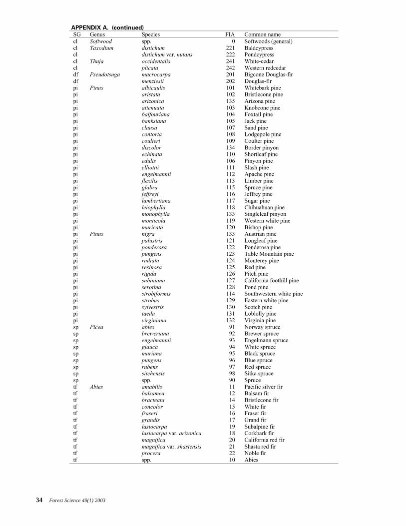
34 Forest Science 49(1) 2003
APPENDIX A. (continued)SG Genus Species FIA Common namecl Softwood spp. 0 Softwoods (general)cl Taxodium distichum 221 Baldcypresscl distichum var. nutans 222 Pondcypresscl Thuja occidentalis 241 White-cedarcl plicata 242 Western redcedardf Pseudotsuga macrocarpa 201 Bigcone Douglas-firdf menziesii 202 Douglas-firpi Pinus albicaulis 101 Whitebark pinepi aristata 102 Bristlecone pinepi arizonica 135 Arizona pinepi attenuata 103 Knobcone pinepi balfouriana 104 Foxtail pinepi banksiana 105 Jack pinepi clausa 107 Sand pinepi contorta 108 Lodgepole pinepi coulteri 109 Coulter pinepi discolor 134 Border pinyonpi echinata 110 Shortleaf pinepi edulis 106 Pinyon pinepi elliottii 111 Slash pinepi engelmannii 112 Apache pinepi flexilis 113 Limber pinepi glabra 115 Spruce pinepi jeffreyi 116 Jeffrey pinepi lambertiana 117 Sugar pinepi leiophylla 118 Chihuahuan pinepi monophylla 133 Singleleaf pinyonpi monticola 119 Western white pinepi muricata 120 Bishop pinepi Pinus nigra 133 Austrian pinepi palustris 121 Longleaf pinepi ponderosa 122 Ponderosa pinepi pungens 123 Table Mountain pinepi radiata 124 Monterey pinepi resinosa 125 Red pinepi rigida 126 Pitch pinepi sabiniana 127 California foothill pinepi serotina 128 Pond pinepi strobiformis 114 Southwestern white pinepi strobus 129 Eastern white pinepi sylvestris 130 Scotch pinepi taeda 131 Loblolly pinepi virginiana 132 Virginia pinesp Picea abies 91 Norway sprucesp breweriana 92 Brewer sprucesp engelmannii 93 Engelmann sprucesp glauca 94 White sprucesp mariana 95 Black sprucesp pungens 96 Blue sprucesp rubens 97 Red sprucesp sitchensis 98 Sitka sprucesp spp. 90 Sprucetf Abies amabilis 11 Pacific silver firtf balsamea 12 Balsam firtf bracteata 14 Bristlecone firtf concolor 15 White firtf fraseri 16 Fraser firtf grandis 17 Grand firtf lasiocarpa 19 Subalpine firtf lasiocarpa var. arizonica 18 Corkbark firtf magnifica 20 California red firtf magnifica var. shastensis 21 Shasta red firtf procera 22 Noble firtf spp. 10 Abies
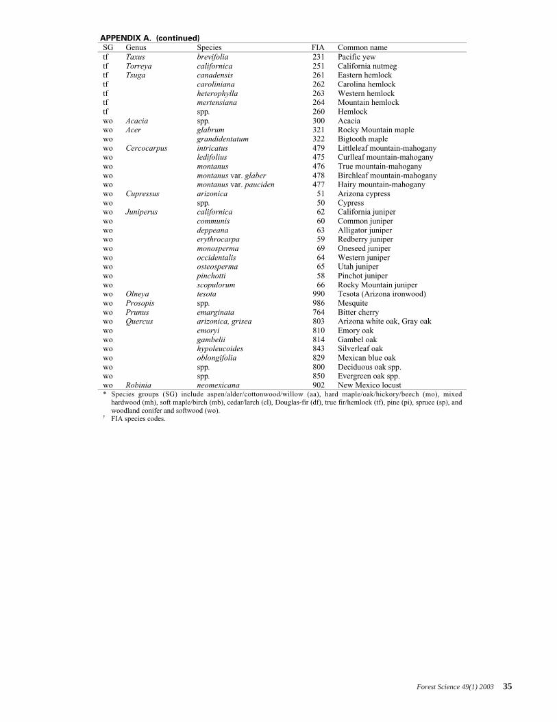
Forest Science 49(1) 2003 35
APPENDIX A. (continued)SG Genus Species FIA Common nametf Taxus brevifolia 231 Pacific yewtf Torreya californica 251 California nutmegtf Tsuga canadensis 261 Eastern hemlocktf caroliniana 262 Carolina hemlocktf heterophylla 263 Western hemlocktf mertensiana 264 Mountain hemlocktf spp. 260 Hemlockwo Acacia spp. 300 Acaciawo Acer glabrum 321 Rocky Mountain maplewo grandidentatum 322 Bigtooth maplewo Cercocarpus intricatus 479 Littleleaf mountain-mahoganywo ledifolius 475 Curlleaf mountain-mahoganywo montanus 476 True mountain-mahoganywo montanus var. glaber 478 Birchleaf mountain-mahoganywo montanus var. pauciden 477 Hairy mountain-mahoganywo Cupressus arizonica 51 Arizona cypresswo spp. 50 Cypresswo Juniperus californica 62 California juniperwo communis 60 Common juniperwo deppeana 63 Alligator juniperwo erythrocarpa 59 Redberry juniperwo monosperma 69 Oneseed juniperwo occidentalis 64 Western juniperwo osteosperma 65 Utah juniperwo pinchotti 58 Pinchot juniperwo scopulorum 66 Rocky Mountain juniperwo Olneya tesota 990 Tesota (Arizona ironwood)wo Prosopis spp. 986 Mesquitewo Prunus emarginata 764 Bitter cherrywo Quercus arizonica, grisea 803 Arizona white oak, Gray oakwo emoryi 810 Emory oakwo gambelii 814 Gambel oakwo hypoleucoides 843 Silverleaf oakwo oblongifolia 829 Mexican blue oakwo spp. 800 Deciduous oak spp.wo spp. 850 Evergreen oak spp.wo Robinia neomexicana 902 New Mexico locust* Species groups (SG) include aspen/alder/cottonwood/willow (aa), hard maple/oak/hickory/beech (mo), mixed
hardwood (mh), soft maple/birch (mb), cedar/larch (cl), Douglas-fir (df), true fir/hemlock (tf), pine (pi), spruce (sp), andwoodland conifer and softwood (wo).
† FIA species codes.