National Income Accounting When Firms Insure Managers:

Understanding Firm Size and Compensation Inequality.

Barney Hartman-GlaserUCLA Anderson

Hanno LustigStanford GSB and NBER

Mindy X. ZhangUT Austin McCombs

June 24, 2016∗

Abstract

We develop a model in which firm-specific shocks have a first-order effect on the distributionof rents between shareholders and managers. In our model, firms optimally provide managerswith contracts that do not expose them to risk. Consequently, larger and more productive firmsreturn a larger share of rents to shareholders while less productive firms endogenously exit. Anincrease in firm-level risk lowers the threshold at which firms exit and increases the measure offirms in the right tail of the size distribution. As a result, such an increase always increasesthe aggregate capital share in the economy, but may lower the average firm’s capital share.Moreover, the aggregate capital share reported in national income accounts produces a biasedestimate of the ex-ante distribution of rents because the data only contain surviving firms. Weconfirm that the average firm’s capital share has declined amongst publicly traded U.S. firms,even though the aggregate capital share has increased. We attribute the secular increase in theaggregate capital share amongst these firms to an increase in firm size inequality that resultsfrom an increase in firm-level risk. This effect is only partially mitigated by an increase ininter-firm labor compensation inequality.

Keywords: Idiosyncratic Risk, Selection, Capital Share, Labor Share, National IncomeAccounting, Selection.

∗Hartman-Glaser: UCLA Anderson School of Management, 110 Westwood Plaza, Los Angeles, CA 90034 (bh-glaser@anderson.ucla.edu). Lustig: Lustig: Stanford Graduate School of Business, 355 Knight Way, Stanford, Ca94305 (hlustig@stanford.edu). Zhang: UT McCombs School of Business, 2110 Speedway B6600, Austin, TX 78712(xiaolan.zhang@mccombs.utexas.edu). We received detailed feedback from Hengjie Ai, Alti Aydogan, Frederico Belo,Bob Hall, Ben Hebert, Chad Jones, Pat Kehoe, Arvind Krishnamurthy, Pablo Kurlat, Ed Lazear, Chris Tonetti,Sebastian DiTella, Andres Donangelo and Andy Skrypacz. The authors acknowledge comments received from sem-inar participants at the Stanford GSB , UT Austin, Universite de Lausanne and EPFL, the Carlson School at theUniversity of Minnesota and the 2016 labor and finance group meeting.

1 Introduction

Over the last decades, publicly traded U.S. firms have experienced a large increase in firm-

specific volatility of both firm-level cash flow as well as returns (see, e.g., Campbell, Lettau,

Malkiel, and Xu, 2001; Comin and Philippon, 2005; Zhang, 2014; Bloom, 2014; Herskovic, Kelly,

Lustig, and Van Nieuwerburgh, 2015). At the same time, the aggregate capital share of these

firms as also increased. We present an equilibrium model which links these two facts and provides

novel implications for national income accounting. We find that the increase in firm size inequality

induced by the increase in risk is the main driver of the increase in the aggregate capital share for

publicly traded firms. The capital share at the average firm, however, has decreased. Inter-firm

compensation inequality has increased (see Song, Price, Guvenen, Bloom, and von Wachter (2015)),

but not enough to offset the effect of the increase the firm size inequality on the capital share.

Since shareholders of publicly traded firms can diversify idiosyncratic firm-specific risk away,

while risk-averse workers cannot, it is efficient for firms to provide managers with insurance against

firm-specific risk. We analyze a simple compensation contract in an equilibrium model of indus-

try dynamics (see, e.g., Hopenhayn, 1992) that pays managers a fixed wage while allocating the

remainder of profits to shareholders. The level of managerial compensation is set in equilibrium

by the value of ex-ante identical firms. Ex-post these firms are subject to permanent idiosyncratic

shocks that lead some firms to increase in size and productivity while others decrease and poten-

tially exit. We use this model as a laboratory to analyze the impact of changes in firm-level risk

on the distribution of rents.

Standard national income accounting applied inside this model yields a new perspective on

capital share dynamics. The manager’s compensation is set such that the net present value of

starting a new firm, computed by integrating over all paths using the density for a new firm,

is zero, but the national income accounts only integrate over all firms that are currently active

using the stationary size distribution, without discounting. As a result, the aggregate capital share

calculation puts more probability mass on the right tail than the NPV calculation. As firm-level

risk increases and the right tail of the firm size distribution grows, managers capture a smaller

1

fraction of aggregate rents ex post, even though they capture all of the ex ante rents. This effect is

partly offset by a larger mass of unprofitable firms in the left tail of the stationary size distribution,

but, in our model, an increase in firm-level risk invariably increases the capital share. Only when

managers receive equity-only compensation is the capital share invariant to changes in firm-level

volatility.

At the heart of this mechanism is the selection effect that arrises by measuring the distribution

of rents excluding firms that have endogenously exited.1 This effect is closely related to Hopenhayn

(2002)’s observation that selection biases average Tobin’s Q estimates for industries above one. In

a similar manner, the capital share computed in national income accounts also produces a biased

estimate of the ex ante profitability of new firms. Moreover, an increase in selection increases the

size of the bias. This effect explains the measured divergence between aggregate compensation and

profits: Compensation is tied to ex ante profitability, not the ex post realized one. This result

also has a natural insurance interpretation. When idiosyncratic risk increases, managers effectively

pay a larger idiosyncratic insurance premium to shareholders ex post. The increase in the ex post

premium leads to an increase in the aggregate capital share, even though the shareholders are risk-

neutral and receive zero rents ex ante. This mechanism has interesting cross-sectional implications.

Only the capital share of the largest firms in the right tail increases as risk increases, but they

determine aggregate capital share dynamics, echoing Gabaix (2011)’s observation that we need to

study the behavior of large firms to understand macroeconomic aggregates. The capital share of

the smallest firms will actually decrease. As a result, the average capital share across all firms will

tend to decrease.

Between 1960 and 2010, the U.S. labor share of total output in the non-farm business sector

of the U.S. economy has shrunk by 15 percent (see Figure 1). This phenomenon does not seem

limited to the U.S. (see, e.g., Piketty and Zucman (2014)). In the universe of U.S. publicly traded

firms, we find that the shrinkage in the labor (capital) share is concentrated among the largest

(smallest) firms in the U.S. In fact, the equal-weighted average labor (capital) share of publicly

1Jovanovic (1982) is the first study of selection in an equilibrium model of industry dynamics. Selection has alsobeen found to be quantitatively important. Luttmer (2007) attributes about 50 percent of output growth to selectionin a model with firm-specific productivity improvements, selection of successful firms and imitation by entrants.

2

traded companies has increased (decreased), starting in the 80s. This new cross-sectional evidence

is consistent with the selection mechanism: The divergence between the average and the aggregate

labor share is a key prediction of selection. The main competing hypothesis is that firms are

increasingly substituting capital for labor (see, e.g., Karabarbounis and Neiman, 2013) in response

to declines. As far as we know, this mechanism does not predict a divergence between the average

and aggregate labor share that we document in the data.

Firm-level risk and the firm size inequality that results plays a key role in U.S. factor share

dynamics. Consistent with the selection mechanism, we find that the decline in the aggregate U.S.

labor share for publicly traded firms cannot be attributed to the averages of log firm-level output

and log compensation, but is entirely due to differential changes in the higher-order moments of

the cross-sectional firm size and firm compensation distribution, as predicted by our model. In

particular, starting in the late seventies, the increases in the variance and kurtosis of the log output

distribution are not matched by similar risk increases for log compensation. An increase in firm

size inequality that is unmatched by a commensurate increase in inter-firm compensation inequality

mechanically lowers the aggregate labor income share. Even though inter-firm wage inequality has

increased, as was recently pointed out by Song et al. (2015), the increase was too small to offset

the increase in firm size inequality.

In a series of papers, Luttmer (2007, 2012) characterizes the stationary size distribution of

firms when firm-specific productivity is subject to permanent shocks. Firms incur a fixed cost

of operating a firm. The selection effect of exit at the bottom of the distribution informs the

shape of the stationary size distribution, which is Pareto with an endogenous tail index. Our

work explores the impact of changes in the stationary size distribution on the distribution of rents

in our laboratory economy. In recent work, Perla, Tonetti, Benhabib, et al. (2014) examine the

endogenous productivity distribution in an environment where firms choose to innovate, adopt new

technology or keep producing with the old technology.

There is a large literature on optimal risk sharing contracts between workers and firms (see

Thomas and Worall, 1988; Holmstrom and Milgrom, 1991; Kocherlakota, 1996; Lustig, Syverson,

and Nieuwerburgh, 2011; Berk and Walden, 2013; Zhang, 2014). This literature has analyzed the

3

1960 1970 1980 1990 2000 20100.3

0.4

0.5

0.6

0.7

Valu

e A

dded

0.12

0.14

0.16

0.18

Sale

s

Cap/Sales

Cap/VA

Figure 1. Capital Share.The figure presents the aggregate capital share in Compustat public firms database. Source:Compustat Fundamentals Annual (1960-2014). We plot two measures: (1) Aggregate capital

share =∑iOperating Incomei∑

iVAifor each year, (2) Aggregate capital share =

∑iOperating Incomei∑

i Salesi.

VAi = Operating Incomei + Labor Costi.

1960 1970 1980 1990 2000 2010

0.3

0.4

0.5

0.6

0.7

Valu

e A

dded

0.1

0.12

0.14

0.16

0.18

0.2

0.22

0.24

Sale

s

Lab/Sales

Lab/VA

Figure 2. Labor Share.The figure presents the aggregate labor share in Compustat public firms database. Source:Compustat Fundamentals Annual (1960-2014). We plot two measures: (1) Aggregate labor

share =∑iLabor Costi∑

iVAifor each year, (2) Aggregate labor share =

∑iLabor Costi∑

i Salesi. VAi =

Operating Incomei + Labor Costi.

4

trade-off between insurance and incentives. We analyze the case of two-sided limited commitment

on the part of the firm and the manager, similar to Ai and Li (2015); Ai, Kiku, and Li (2013). When

we introduce moral hazard and other frictions, our mechanism will be mitigated. However, we show

that when we allow workers to have some exposure to firm performance, our primary results remain

unchanged. The intuition is that so long as a firm’s owners are providing some insurance to it’s

workers, and can exit when productivity declines, the selection problem still applies. Gabaix and

Landier (2008); Edmans, Gabaix, and Landier (2009) examine equilibrium CEO compensation in

a competitive market for CEO talent. The equilibrium compensation will be comprised of a cash

component and an equity component. We analyze the implications of this class of contracts for our

key results.

The rest of this paper is organized as follows. Section 2 present empirical evidence on U.S.

capital share dynamics. Section 3 describes the benchmark model that we use as a laboratory.

Section 4 derives the stationary firm size distribution in the benchmark model, and it describes the

implications for the aggregate capital share. Section 5 considers a large class of compensation con-

tracts that allow for performance sensitivity. Finally, section 6 considers a version of our economy

with production and unskilled labor.

2 Understanding U.S. Capital Share Dynamics

In this section, we present empirical evidence on the joint dynamics of compensation, firm size

and the implied capital share dynamics. We show the findings are consistent with the selection

mechanism.

2.1 Data

Our baseline results are from analyzing two sources of data. To obtain cross-sectional evidence,

we use widely available accounting data from Compustat Fundamentals Annual, which includes all

publicly-traded firms. The sample is from 1960 to 2014. We exclude financial firms with SIC codes

in the interval 6000-6799, and also exclude firms whose sales, employee numbers and total asset

5

values are negative. We examine the distribution of factor share of output in the publicly traded

firm sample.

The capital income of the firm is measured by operating income before depreciation (OIBDP).

OIBDP represents sales/turnover (SALE) minus operating expenses including the cost of goods

sold, labor cost and other administrative expenses. Capital share of output is the ratio of OIBDP

to sales2.

We use the ratio of the cost of labor to sales as the measure of labor share of output. The

cost of labor is the staff expenses – total (XLR) in Compustat. However, the limitation of XLR

is that XLR in Compustat is sparse with roughly 13% firm-year observations in the sample. We

then follow Donangelo, Gourio, and Palacios (2015) to construct the extended labor cost. We first

estimate the average labor cost per employee (XLR/EMP) within industry for each year using the

available XLR observations, and then labor cost of a firm with missing XLR equals the number of

employees times the average labor cost per employee of the same industry3 during that year.

For both the labor share and capital share calculation, value added (VA) is the ideal denomi-

nator. Although the labor cost is sparsely reported in the public firm sample, we use our extended

XLR to construct a firm-level measure of value added VAi, which equals to OIBDP plus Extended

XLR. Although value added can be negative for the individual firm on the tail of firm size distribu-

tion, hence it is not sensible to calculate factor shares scaling by value added, we use the estimates

of VAi to compute the aggregate factor share as a robustness check. Figure 1 presents the time

series of our two measures of aggregate capital share.

2.2 Capital Share Dynamics

In this section, we examine the capital share dynamics over time. Firm level volatility has

increased over the past five decades (Comin and Philippon (2005), Zhang (2014), Herskovic et al.

(2015)). Figure 3 confirms the time series results of firm-level volatility. The measure of cash flow

2Ideally, capital share should be computed using value added as denominator. However, the cost of material andthe cost of labor are not reported separately in the sample. Instead of using different ways to estimate the cost oflabor or the cost of material which leads to many negative value added at the tail, we will stick to sales as the measureof output.

3We follow Donangelo et al. (2015) and use Fama-French 17 industry classifications. The result is robust using2-digit SIC code.

6

1950 1960 1970 1980 1990 2000 2010-3

-2.5

-2

-1.5

-1

Log V

ola

tilit

y (

Sale

s G

row

th)

-4.5

-4

-3.5

-3

-2.5

Log V

ola

tilit

y (

Retu

rns)

Idiosyncratic Returns

Sales Growth

Figure 3. Firm Level Volatility of U.S. Public Firms

The dashed line is annualized idiosyncratic firm-level stock return volatility. Idiosyncratic returnsare constructed within each calendar year by estimating a Fama French 3-factor model using allobservations within the year. Idiosyncratic volatility is then calculated as the standard deviationof residuals of the factor model within the calendar year. We obtain the time series of idiosyncraticvolatility by average across firms at each year. The solid line is the firm-level cash flow volatility,estimated for all CRSP/Compustat firms using the 20 quarterly year-on-year sales growth obser-vations for calendar years. The idiosyncratic sales growth is the standard deviation of residualsof a factor specification. The factors for sales growth are the first 3 major principal components.Source: CRSP 1960-2014 and Compustat Fundamentals Annual 1950-2014.

volatility and stock return volatility has almost doubled over the period 1960-2010. The rising

firm-level volatility is a very robust fact using other firm-level variables (Comin and Philippon

(2005)).

For most of our analysis, we focus on the capital share of output. Figure 4 plots the average and

aggregate capital share in the publicly traded firm sample. The average capital share is the sample

mean of capital share for a given year. As the firm-level volatility increases, the aggregate capital

share and the average capital share diverge. The aggregate capital share equals the sum of capital

income (OIBDP) across all the firms divided by aggregate sales. The average capital share drops

from 0.13 in 1960 to -0.40 in 2014, while the aggregate capital share increases with a less dramatic

scale, from 0.14 in 1960 to 0.17 in 2014. The presence of the contrasting trends in capital share

is consistent with the mechanism we highlight in our model. Specifically, the trends we observe in

7

1960 1970 1980 1990 2000 2010-0.6

-0.4

-0.2

0

0.2

Avera

ge

0.14

0.16

0.18

Aggre

gate

Aggregate Trend

Aggregate

Average Trend

Average

Figure 4. Average and Aggregate Capital ShareCapital share of output equals the ratio of operating income to sales. Aggregate capital share =∑

iOperating Incomei∑i Salesi

for each year. Average capital share = mean(Operating Income

Sales) for each

year. The dash lines are the HP-filtered trends. Source: Compustat Fundamentals Annual (1960–2014).

the data a consistent with changes in firm-level volatility causing a shift in the distribution of firm

size that favors the owners of capital

We find similar patterns in the labor share dynamics. The aggregate labor share of output in

the non-farm business sector has declined by 15%. However, the the trend of the average labor

share of output in the publicly traded firm sample did not decline. Figure 5 shows the time series of

both the average and the aggregate labor share in our sample using the estimated labor cost. The

average labor share rises from 0.32 in 1960 to 0.4 in 2014, while the aggregate labor share drops

from 0.25 to 0.19 during the same period of time.

2.3 Firm Size and Firm Compensation Inequality

Firm-level risk and firm size inequality are the key drivers of U.S. labor share and capital share

dynamics. We can use the cumulant generating function to decompose capital share dynamics. The

aggregate labor share is the ratio of two cross-sectional moments: 1−Π = E(lab)E(sales) where Π denotes

the aggregate capital share. We can decompose these cross-sectional moments using higher-order

8

1960 1970 1980 1990 2000 20100.25

0.3

0.35

0.4

Ave

rag

e

0.1

0.15

0.2

0.25

Ag

gre

ga

te

Aggregate Trend

Aggregate

Average Trend

Average

Figure 5. Aggregate and Average Labor Share of U.S. Public FirmsThe figure presents the average and aggregate labor share in Compustat public firms database.Labor share is measured by the ratio of estimated staff expenses (XLR) to sales. The dashedlines are the HP-filtered trends of the average and the aggregate labor share. Source: CompustatFundamentals Annual (1960-2014).

moments of the log sales and log labor income distribution. In particular, we can expand the log

of the aggregate labor share as the difference in the cumulant-generating functions of log output

and log capital at the firm level:

log(1−Π) = logE(lab)− logE(sales) =∞∑j=1

κj(log lab)

j!−∞∑j=1

κj(log sales)

j!, (1)

where the cumulants are defined by:

mean : κ1,

variance : κ2,

skewness : κ3/κ3/22 ,

kurtosis : κ4/κ22.

We decompose the aggregate labor share instead of the capital share because labor income is

9

non-negative. Figure 6 plots the difference in the cross-sectional cumulants of log sales and log

labor income. The log of labor income is approximated by log of sales minus operating income

before depreciation log(Sales − OIBDP ), because the labor data is sparse. The sum of all these

weighted differences in cumulants adds up the log labor income share. The means of the log sales

and log labor income distribution do not contribute much to the decline in the labor income share.

All of the time series variation in the aggregate labor share is induced by higher order moments.

Note that a common measure of risk is the entropy of a random variable L(x) = log(E(x))−E log(x).

Hence, much of the change in the aggregate labor share is attributable to difference in entropy

between firm size (sales) and firm labor income.

∆ log(1−Π) ≈ L(lab)− L(sales) =∞∑j=2

κj(log lab)

j!−∞∑j=2

κj(log sales)

j!

We can interpret L(lab) as a measure of inter-firm compensation inequality, and L(sales) as a

measure of firm size inequality. The log of aggregate labor income share in this sample declines

because the overall cross-sectional inequality in labor compensation increases far less than the

overall inequality in the size distribution. Table 1 provides a decade-by-decade overview of all four

cumulants for sales and labor income. The top panel considers all sectors, including financials. The

bottom panel considers only non-financials. Across-the-board, both for sales and compensation, we

see large increase in variance and kurtosis starting in the seventies, together with large increases

in negative skewness. However, these increases are much larger for sales than for labor income.

Between 1960 and 2014, we record a 279 log point increase in the cumulant sum for firm sales, but

only 208 log points for compensation, which implies a 71 log point increase in the difference between

the size and compensation weighted sum of cumulants. Table 2 reports the differences between the

moments of the compensation and size distribution. The last column shows that 69 log points are

due to the difference in firm size and firm compensation inequality (≈ L(lab) − L(sales)). In this

sample, the changes in the means have no bearing on the aggregate labor share. When we exclude

financials, reported in the bottom panel, the results are even stronger. Changes in the means do

not account for any of the labor share decline.

10

Basically, the increase in the cross-sectional variance and kurtosis of the log size distribution

that started in the late 70s in our universe of firms is not matched by similar changes in the log

labor compensation distribution. These forces are only partly mitigated by an increase in negative

skewness of the log size distribution, because of a growing mass of small, unprofitable firms in the

left tail of the size distribution, that is not offset a similar increase in the log labor compensation

distribution. As documented by Fama and French (2004), the wave of new listings that started in

1980 gave rise to a large mass of unprofitable firms in the tail of the size distribution. The increasing

left skewness of profitability and right skewness of growth after 1979 are not due to younger firms

seeking a public listing: Loughran and Ritter (1995) conclude that during 1980-1998 there is no

downtrend in the average age of firms going public. Starting in 1996, this trend in new listings

reversed itself, and there was a sharp decline in the number of listed firms (Doidge, Karolyi, and

Stulz (2015)). The decline is concentrated mostly in smaller firms.

1960 1970 1980 1990 2000 2010 2020

Year

-2.5

-2

-1.5

-1

-0.5

0

0.5

1

1.5

2

κ1(log(lab))− κ1(log(sales))12κ2(log(lab))−

12κ2(log(sales))

16κ3(log(lab))−

16κ3(log(sales))

124κ4(log(lab))−

124κ4(log(sales))

Figure 6. Cross-sectional Cumulants of Firm-level Compensation and SizeThe plot shows the first four cumulants of the log labor compensation minus the same cumulantsfor the log sales distribution. Labor compensation is approximated at the firm level as Sales minusoperating income before depreciation (OIBDP). The sample includes all Compustat firms (bothactive and inactive), 1960-2014. The sample is winsorized at 1%.

11

Table 1. Firm Size and Compensation Inequality

Periods Panel A: Including Financials

κ1κ22

κ33!

κ44!

∑4j=1

κjj!

∑4j=2

κjj!

Sales

1960 - 1969 4.560 1.208 0.027 0.019 5.814 1.2551970 - 1979 4.367 1.610 -0.014 0.243 6.205 1.8391980 - 1989 4.068 3.138 -0.841 0.549 6.915 2.8471990 - 1999 4.541 2.704 -0.334 0.571 7.482 2.9412000 - 2009 5.445 2.665 -0.470 0.566 8.206 2.761

2010 - present 5.968 2.693 -0.932 0.876 8.605 2.637

2010’s-1960’s 1.408 1.485 -0.959 0.857 2.791 1.382

Labor Compensation

1960 - 1969 4.384 1.242 0.008 0.032 5.666 1.2821970 - 1979 4.192 1.647 0.006 0.110 5.954 1.7631980 - 1989 3.954 2.793 -0.041 -0.385 6.320 2.3661990 - 1999 4.421 2.338 0.332 -0.122 6.969 2.5482000 - 2009 5.332 2.265 0.287 -0.210 7.674 2.343

2010 - present 5.774 2.358 0.086 -0.472 7.746 1.972

2010’s-1960’s 1.390 1.116 0.077 -0.504 2.080 0.689

Periods Panel B: Excluding Financials

Sales

1960 - 1969 4.585 1.183 0.051 0.014 5.833 1.2471970 - 1979 4.387 1.584 0.017 0.265 6.254 1.8661980 - 1989 4.055 3.094 -0.799 0.606 6.956 2.9011990 - 1999 4.586 2.783 -0.490 0.614 7.493 2.9072000 - 2009 5.549 2.794 -0.834 0.716 8.224 2.676

2010 - present 6.134 2.785 -1.388 1.213 8.743 2.610

2010’s-1960’s 1.548 1.602 -1.439 1.199 2.911 1.362

Labor Compensation

1960 - 1969 4.413 1.208 0.046 0.010 5.676 1.2631970 - 1979 4.234 1.575 0.092 0.088 5.988 1.7551980 - 1989 3.977 2.669 0.058 -0.290 6.415 2.4371990 - 1999 4.528 2.267 0.345 -0.173 6.967 2.4392000 - 2009 5.506 2.160 0.222 -0.267 7.621 2.115

2010 - present 5.999 2.189 -0.007 -0.413 7.768 1.769

2010’s-1960’s 1.586 0.981 -0.053 -0.422 2.092 0.506

The table shows the first four cumulants of the log labor compensation minus the same cumulantsfor the log sales distribution. Labor compensation is approximated at the firm level as Sales minusoperating income before depreciation (OIBDP). The sample includes all Compustat firms (bothactive and inactive), 1960-2014. The sample is winsorized at 1%.12

Tab

le2.

Tim

eS

erie

sof

Cu

mu

lants

(Fu

llS

amp

le):

log

lab

sales

and

logoibdp

sales

Per

iod

sP

anel

A:

Incl

ud

ing

Fin

anci

als

κ1(l

oglab)

κ2(l

oglab)

2κ3(l

oglab)

3!

κ4(l

oglab)

4!

∑ 4 j=1κj(l

oglab)

j!

∑ 4 j=2κj(l

oglab)

j!

−κ

1(l

ogsales)−κ2(l

ogsales)

2−κ3(l

ogsales)

3!

−κ4(l

ogsales)

4!

−∑ 4 j=

1κj(l

ogsales)

j!−∑ 4 j=

2κj(l

ogsales)

j!

196

0-

1969

-0.1

76

0.03

4-0

.019

0.01

3-0

.148

0.02

8197

0-

1979

-0.1

75

0.03

70.

020

-0.1

33-0

.251

-0.0

76198

0-

1989

-0.1

14

-0.3

460.

800

-0.9

35-0

.594

-0.4

80199

0-

1999

-0.1

20

-0.3

660.

666

-0.6

93-0

.513

-0.3

93200

0-

2009

-0.1

14

-0.4

000.

757

-0.7

76-0

.532

-0.4

18201

0-

pre

sent

-0.1

94

-0.3

351.

018

-1.3

48-0

.859

-0.6

652010

’s-1

960

’s-0

.018

-0.3

691.

037

-1.3

60-0

.711

-0.6

93

Per

iod

sP

anel

B:

Excl

ud

ing

Fin

anci

als

κ1(l

oglab)

κ2(l

oglab)

2κ3(l

oglab)

3!

κ4(l

oglab)

4!

∑ 4 j=1κj(l

oglab)

j!

∑ 4 j=2κj(l

oglab)

j!

−κ

1(l

ogsales)−κ2(l

ogsales)

2−κ3(l

ogsales)

3!

−κ4(l

ogsales)

4!

−∑ 4 j=

1κj(l

ogsales)

j!−∑ 4 j=

2κj(l

ogsales)

j!

196

0-

1969

-0.1

73

0.02

5-0

.005

-0.0

04-0

.157

0.01

6197

0-

1979

-0.1

54

-0.0

090.

075

-0.1

77-0

.265

-0.1

12198

0-

1989

-0.0

78

-0.4

250.

857

-0.8

96-0

.542

-0.4

64199

0-

1999

-0.0

58

-0.5

160.

835

-0.7

87-0

.526

-0.4

68200

0-

2009

-0.0

43

-0.6

341.

057

-0.9

83-0

.603

-0.5

60201

0-

pre

sent

-0.1

35

-0.5

961.

381

-1.6

26-0

.975

-0.8

412010

’s-1

960

’s0.

038

-0.6

211.

386

-1.6

22-0

.819

-0.8

57

Th

eta

ble

show

sth

ed

iffer

ence

sin

the

firs

tfo

ur

cum

ula

nts

ofth

elo

gla

bor

com

pen

sati

onm

inu

sth

esa

me

cum

ula

nts

for

the

log

sale

sd

istr

ibu

tion

.L

abor

com

pen

sati

onis

app

roxim

ated

atth

efi

rmle

vel

asS

ales

min

us

oper

atin

gin

com

eb

efor

ed

epre

ciat

ion

(OIB

DP

).T

he

sam

ple

incl

ud

esall

Com

pu

stat

firm

s(b

oth

acti

ve

an

din

acti

ve),

1960

-201

4.T

he

sam

ple

isw

inso

rize

dat

1%.

13

Figure 7 plots the weighted fourth cumulants by industry. This plot shows that the increase in

kurtosis of firm size unmatched by firm compensation is broad-based across industries, but seems

most pronounced in high-tech and manufacturing, and smaller in health and consumer goods.

1960 1970 1980 1990 2000 2010 2020

Year

-3.5

-3

-2.5

-2

-1.5

-1

-0.5

0

0.5

1

124κ4(log(lab))−

124κ4(log(sales))

Full Sample (Non Financials)

Consumer Goods

Manufacturing

High Tech

Health

Figure 7. Fourth Cumulants of Compensation and Size by IndustryThe plot shows the fourth cumulant of the log labor compensation minus the fourth cumulant of thelog sales distribution computed by industry. Labor compensation is approximated at the firm levelas Sales minus operating income before depreciation (OIBDP). The sample includes all Compustatfirms (both active and inactive), 1960-2014. The sample is winsorized at 1%.

2.4 Cross Sectional Variation in Capital Share Dynamics

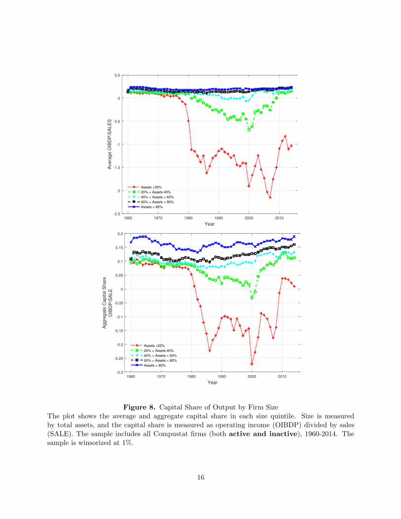
Figure 8 presents the average and aggregate capital share for difference size groups. All firms

are sorted into five groups based on their total assets. Within each group, we compute the aver-

age capital share. The average capital share tends to decline more in the smaller size quintiles.

Aggregate capital share increases in total, but the increase in profitability mainly happens in the

larger firms. Over the period from 1960 to 2014, firm-level volatility has gone up, and hence small

firms with low profitability stay in the industry as they find the abandon options are more valuable.

During the same period, we find that the capital share of the large firms (group 5) remains stable.

14

The dispersion of capital share across size groups increases over time as the volatility increases.

Changes in the capital share of firms on the right tail of size distribution imply the change in the

selection process of the public firms. Consistently, we see that the average capital share of firms

that were liquidated is declining over time (Figure 14). We then compare the average and aggregate

factor share of output for different volatility sectors. Figure 12 presents the time series of factor

shares for low volatility and high volatility sectors. Panel (a) reports the trends of OIBDP to Sales

ratio. The divergence of average and aggregate trends only presents in the high volatility sectors.

In Figure 13, the decline of capital share in the small firms group (group 1) is much more sizable

in the high volatility sector than in the low volatility sector.

To address the concern of changing composition of public firm sample, we examine the distri-

bution of capital share controlling for industries. We examine four main industries in this paper:

consumer goods, manufacturing, health products and information, computer and technology (high

tech) industry. The definition of consumer goods, manufacturing and health products are taken

from Fama-French 5 industry classification. The high tech industry definition is from BEA Industry

Economic Accounts4. We fix the definitions of industries over time, and sort firms into five different

size groups within each industry. We find similar cross-sectional patterns within each industry: the

dispersion of capital share across size groups increases over the last five decades, while the more

significant decline in capital share happens in the smaller size quintiles. We also see stronger selec-

tion effect in the high tech industry and in the health products industry which have relatively high

firm-level volatility.

3 Model

In this section we present a model to rationalize the facts we present above. In the model, firms

produce cash flows according to a simple production function. We abstract from physical capital

and unskilled labor. As we show in Section 6, adding these factors does not change any of the main

results, but does substantially complicate the analysis.

4The high tech industry is classified using NAICS, consisting of computer and electronic products, publishing andsoftware, information and data processing, and computer system design and related services.

15

1960 1970 1980 1990 2000 2010

Year

-2.5

-2

-1.5

-1

-0.5

0

0.5

Ave

rag

e O

IBD

P/S

AL

ES

Assets <20%

20% < Assets 40%

40% < Assets < 60%

60% < Assets < 80%

Assets > 80%

1960 1970 1980 1990 2000 2010

Year

-0.3

-0.25

-0.2

-0.15

-0.1

-0.05

0

0.05

0.1

0.15

0.2

Ag

gre

ga

te C

ap

ita

l S

ha

re

OIB

DP

/SA

LE

Assets <20%

20% < Assets 40%

40% < Assets < 60%

60% < Assets < 80%

Assets > 80%

Figure 8. Capital Share of Output by Firm SizeThe plot shows the average and aggregate capital share in each size quintile. Size is measuredby total assets, and the capital share is measured as operating income (OIBDP) divided by sales(SALE). The sample includes all Compustat firms (both active and inactive), 1960-2014. Thesample is winsorized at 1%.

16

Importantly, the shareholders of a given firm hold an option to cease operations when produc-

tivity falls. This is the classic abandonment option that has been well studied in the real options

literature. As is standard in that literature, increasing the volatility of the firms cash flows increases

the value of the option to wait to abandon, and thus decreases the threshold in productivity at

which the firm ceases operations.

Given the solution to the optimal abandonment problem, we characterize the stationary distribu-

tion of firms. Increasing (idiosyncratic) cash flow volatility leads more firms to delay abandonment

and survive long enough to become very productive. As such, the average across firms of the capital

share of profits can be increasing in volatility.

3.1 Environment

The economy is populated by a measure of ex ante identical firms each operating a unit of

physical capital with productivity Xidt given by

dXi = µXidt+ σXidZi −XidN it ; for Xi > Xmin

where Zi is a standard Brownian motion independent across firms, N i is a Poisson process with

intensity λ, and Xmin > 0 is some minimum level of productivity. If dN it = 1, or of Xi reaches

Xmin, Xi jumps to zero, and the firm exits. The process N it gives rise to what is often referred

to as an exogenous death rate of firms and is necessary to guarantee the existence of a stationary

distribution of firms for all parameterizations of the model. Physical capital is normalized to one

for simplicity for the time being. We also abstract from the use of unskilled labor in production.

In section 6 we enrich the environment to production functions that include physical capital and

unskilled labor. Since all firms produce independent and identically distributed cash flows, we will

drop the i superscript for the remainder of the paper.

Each firm is owned by a shareholder and requires a skilled manager to operate. We assume

shareholders are risk-neutral and discount cash flows at the risk free rate r > µ while managers

17

value a stream of payment {ct}t≥0 according to the following utility function

U({ct}t≥0) = E

[∫ ∞0

e−rtu(ct)dt

],

where u′(c) ≥ 0 and u′′(c) > 0. We normalize the measure of managers in the economy to one.

Firms can exit at the discretion of the shareholder. When a firm exits, its shareholder receives

the liquidation value of the firm, which normalize to zero. There is a competitive fringe of share-

holders waiting to create new firms. When an shareholer creates a new firm, she must match with

a manager then pay a cost P for a new unit of physical capital and the technology to operate it.

After creating a new firm, the firm’s initial productivity is drawn from a Pareto distribution with

density

f(X) =ρ

X1+ρ; X ∈ [Xmin,∞).

This distribution implies that the log-productivity of an entering firm is exponentially distributed

with parameter ρ > 1 and simplifies the characterization of equilibrium that follows. We denote

the rate at which new firms are created by ψt. Note that this implies that the entry rate at a given

point X is ψtf(X).

Upon matching with a manager, a shareholder in a new firm offers a long term contract to the

manager prior to the realization of the firm’s productivity and payment of the cost P . The manager

can reject the contract at which point she is instantaneously matched with a new shareholder.

Formally, this contract can be denoted by a process {ct}t≥0 determining payment to the manager

of ct at time t. We assume that the investor cannot commit to continue operations or to pay the

manager once the firm has ceased operations. We also assume that the manager can choose to

exit the contract and match with a new firm at any time and that she does not have access to a

savings technology. When the firm ceases operations, the manager is matched with a entering firm

and signs a new contract. This contracting environment features a two sided limited commitment

problem similar to Ai and Li (2015); Ai et al. (2013). Importantly the outside option of the manager

will depend on the value of starting a new firm, which is endogenously determined in equilibrium.

We denote the utility the manager receives upon entering this market by U0, which is also the

18

manager’s reservation utility. At the inception of the contract, the investor and manager takes U0

as exogenously given, although it will be determined in equilibrium by the market for managers.

The investor will continue operations as long as doing so yields a positive present value. This means

that the investor operating for the firm is the solution to a standard abondonment option common

in the real options literate. Specifically, the investor operates the firm until a stopping time denoted

by τ . The investor’s problem is thus

maxτ,c

E

[∫ τ

0e−rt(Xt − ct)dt

](2)

such that

U0 ≤ E[∫ τ

te−r(s−t)u(cs)ds+ e−r(τ−t)U0

]for all t > 0. (3)

Intuitively, the manager’s limited commitment constraint given in equation (3) must bind as de-

livering more continuation utility to the manager can only ever reduce the investor’s value for the

firm. As a result, the manager value for the contract is constant over time and it is without loss

of generality to restrict attention to contracts that offer the manager a fixed wage c until the firm

exits, at which point the manager reenters the market and receives her outside option. Thus, we

can simplify the investors problem to

V (X; c) = maxτ

E

[∫ τ

0e−rt(Xt − c)dt

], (4)

where V (X; c) is the value of operating a firm with current productivity X given a manager contract

c. The payment c to the manager then acts as a fixed cost or operating leverage. As such, the

investor in a given firm will choose to exit if productivity X is low enough as in the classic problems

of optimal abandonment considered in the real options literature or optimal default as in Leland

(1994). It is without loss of generality to restrict attention to firm exit times that are given by

threshold rules of the form

τ = inf{t|Xt ≤ X or dNt = 1}

19

for some X ≥ 0.

Before stating the definition of equilibrium, it will be useful define xt = log(Xt).

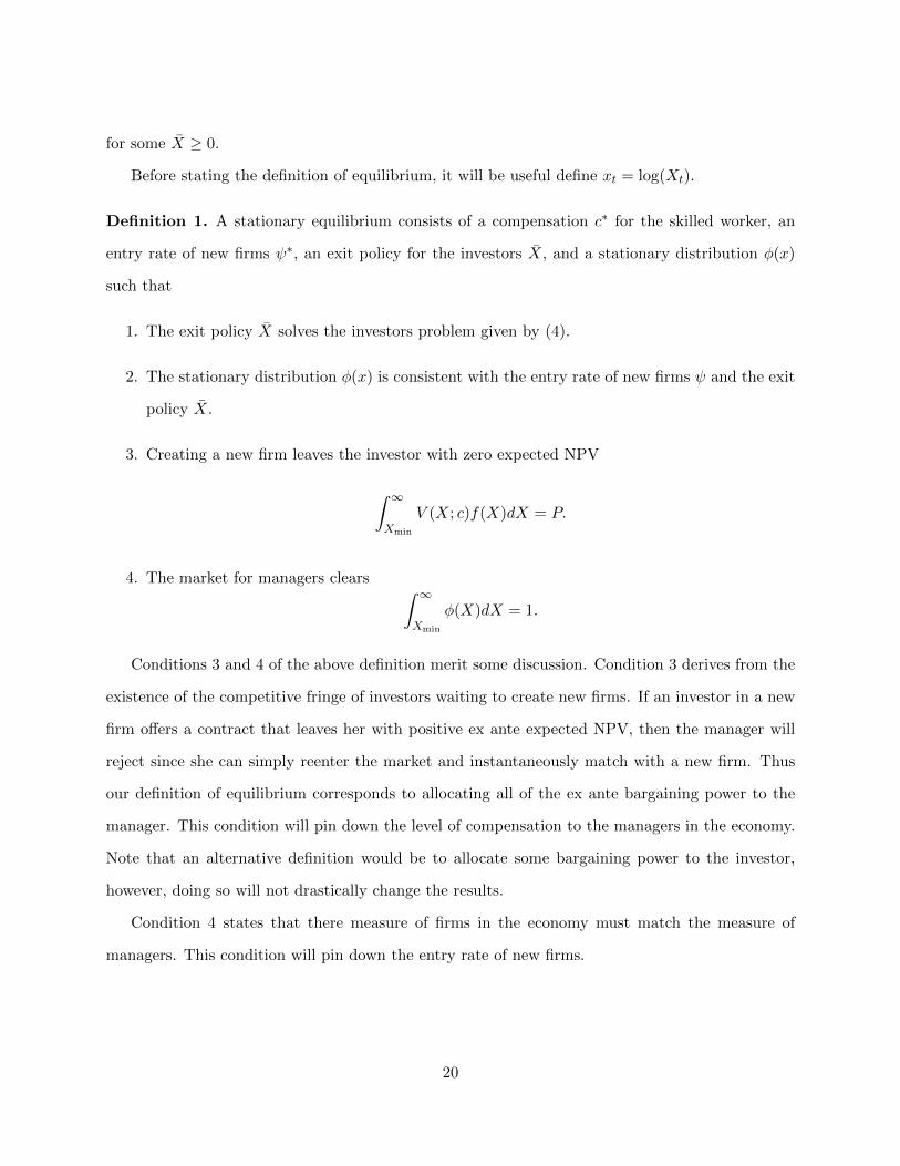
Definition 1. A stationary equilibrium consists of a compensation c∗ for the skilled worker, an

entry rate of new firms ψ∗, an exit policy for the investors X, and a stationary distribution φ(x)

such that

1. The exit policy X solves the investors problem given by (4).

2. The stationary distribution φ(x) is consistent with the entry rate of new firms ψ and the exit

policy X.

3. Creating a new firm leaves the investor with zero expected NPV

∫ ∞Xmin

V (X; c)f(X)dX = P.

4. The market for managers clears ∫ ∞Xmin

φ(X)dX = 1.

Conditions 3 and 4 of the above definition merit some discussion. Condition 3 derives from the

existence of the competitive fringe of investors waiting to create new firms. If an investor in a new

firm offers a contract that leaves her with positive ex ante expected NPV, then the manager will

reject since she can simply reenter the market and instantaneously match with a new firm. Thus

our definition of equilibrium corresponds to allocating all of the ex ante bargaining power to the

manager. This condition will pin down the level of compensation to the managers in the economy.

Note that an alternative definition would be to allocate some bargaining power to the investor,

however, doing so will not drastically change the results.

Condition 4 states that there measure of firms in the economy must match the measure of

managers. This condition will pin down the entry rate of new firms.

20

4 Equilibrium and National Income Accounting

In this section, we characterize the stationary equilibrium of the model and study its implications

for national income accounting.

4.1 Ex Ante Firm Value and the Equilibrium Wage

To solve for the firm value function and exit policy of the investor, we use standard techniques

from the real options literature. An application of Ito’s formula and the dynamic programing

principal imply that V (X; c) must satisfy the following ordinary differential equation

(r + λ)V (X; c) = X − c+ µX∂

∂XV (X; c) +

1

2σ2X2 ∂2

∂X2V (X; c), (5)

with the boundary conditions

V (X(c); c) = 0, (6)

∂

∂XV (X(c); c) = 0, (7)

limX→∞

∣∣∣∣V (X; c)−(

X

r + λ− µ− c

r + λ

)∣∣∣∣ = 0. (8)

Conditions (6) and (7) are the standard value matching and smooth pasting conditions pinning

down the optimal exercise boundary for the abandonment option. Condition (8) arises because as

Xt tends to infinity, abandonment occurs with zero probability and the value of the firm must tend

to the present value of a growing cash flow less a fixed cost.

The solution to equations (5)-(8) is given by

X(c) =η

η + 1

c(r + λ− µ)

r + λ(9)

V (X; c) =X

r + λ− µ− c

r + λ−(

X(c)

r + λ− µ− c

r + λ

)(X

X(c)

)−η(10)

where

η =µ− 1

2σ2 +

√(µ− 1

2σ2)2 + 2(r + λ)σ2

σ2.

21

Note that an increase in firm-level volatility σ invariably lowers the abandonment threshold, simply

because an increase in volatility raises the option value of keeping the firm alive. This feature of

the abandonment option will play key role in our analysis as will become apparent when we discuss

the stationary distribution of firm size. Specifically, an increase in firm-level volatility will lead to

a increase mass of firm’s that delay exit, increasing the mass of firms that have low productivity as

well the mass of firms that survive long enough to achieve high productivity.

Given the solution for firm value conditional on a manager wage c as well as our assumption

on the distribution of productivity of new firms, we can solve for the equilibrium compensation in

closed form. We have

c∗ =

(P (r + λ)(ρ− 1)(ρ− η)

η

(η(r + λ− µ)

(η + 1)(r + λ)

)ρ)− 1ρ−1

. (11)

The derivation of c∗ is given in section of the Appendix.

4.2 The Kolmogorov Forward Equation

We use φ to denote the stationary distribution of x = logX. To remain stationary, the expected

change via inflow and outflow in the measure of firms at a given level of x must be equal to the

measure of firms that exogenously die at the rate λ less the measure of firms that endogenously enter

at the rate ψg(x) (see p. 273 in Dixit and Pindyck, 1994). This leads to the following Kolmogorov

forward equation for φ(x)

1

2σ2φ′′(x)−

(µ− 1

2σ2

)φ′(x)− λφ(x) + ψg(x) = 0. (12)

where

g(x) = ρe−ρx.

22

is the density of initial log productivity x for entering firms. A similarly argument gives a boundary

condition for φ(x) at the exit barrier x = log X

φ(x) = 0. (13)

The final equation that determines the stationary distribution of firm size is given by the market

clearing condition for managers ∫ ∞x

φ(x)dx = 1. (14)

The solution to equations (12)-(14) is given by

φ(x) =ργ

ρ− γ

(e−γ(x−x) − e−ρ(x−x)

)(15)

for x ∈ [x,∞), where

γ =−(µ+ 1

2σ2) +

√(µ− 1

2σ2)2 + 2σ2λ

σ2. (16)

The solution also allows us to characterize the aggregate entry rate of new firms

ψ =γ(ρ(µ+ 1

2σ2)− 1

2ρ2σ2 − λ)

ρ− γeρx. (17)

We note the our assumption on the density of productivity of entering firms allows for the simple

closed form solutions above. The general solution to the ODE given in equation (12) is exponential.

By assuming that g(x) is exponential as well, we are left with a solution to equation (12) for which

it is possible to solve the boundary condition given in equation (13).

Figure 9 plots the stationary distribution of firm productivity for different levels of σ. The other

parameters are calibrated at r = 5%, µ = 2%, λ = .05, ρ = 3, P = 1. As σ increases, the stationary

distribution shifts to the left and becomes more diffuse, with a fatter right tail. The shift to the

left is due to the fact that as firm-level volatility increase, the value of the option to wait to exit

increases, and the optimal point at which the investor chooses to exit necessarily decreases.

The effect of firm-level volatility on the shape of φ(x) visible in figure 9 is born out by examining

23

0 1 2 3 4

0

0.2

0.4

0.6

0.8

x

φ(x)

σ = .1σ = .2σ = .3

3.5 4 4.5 5 5.5

0

2

4

6

8

·10−3

x

φ(x)

σ = .1σ = .2σ = .3

Figure 9. The stationary distribution of log-productivity for σ = .1, .2, and .3. Parameter values:r = 5%, µ = 2%, λ = .05, ρ = 3, p = 1.

the higher-ordered moments of φ(x). Table 3 reports the standard deviation, the skewness and the

kurtosis of the log size distribution as we increase σ. As σ increases, the right skewness increases

from 0.12 to 2.74 and the excess kurtosis of the log size distribution increases from 0.15 to 7.31.

This overall widening of the distribution with a fattening of the left tail comes from two effects.

First there is a direct effect of σ on the dispersion of the distribution of firm size. When firm-

level productitivity is more volatile, the stationary distribution of firms must be more dispersed.

This is evident by examining the dependence of γ on σ. The second effect operates through the

abandonment option. When the option to wait to exit becomes more valuable, more firms delay

exit, and as a result more firms survive long enough to become very productive. As a result the

right tail of the distribution becomes fatter. In the next section, we show that this effect has

important implications for national income accounting.

4.3 Capital Share and Ex Post Profitability

Armed with this stationary distribution, we can do national income accounting inside our model.

We use this stationary distribution to calculate the total and average profit share for a range of σ.

24

Table 3. Higher order moments of the log-size distribution implied by the model

σ Mean Std. Dev. Skew. Kurt.

.1 1.879 0.700 0.120 0.151

.2 1.493 0.696 2.186 5.631

.3 1.181 0.789 2.742 7.310

Moments of the stationary distribution of log-productivity for σ = .1, .2, and .3. Parameter values:r = 5%, µ = 2%, λ = .05, ρ = 3, p = 1.

Specifically, we use the stationary distribution to calculate the aggregate capital share:

Capital Share of Profits = Π =

∫∞x (ex − c)φ(x)dx∫∞

x exφ(x)dx,

= 1−(ρ− 1

ρ

)(γ − 1

γ

)( cX

)

and the average capital share:

Average Capital Share of Profits =

∫ ∞x

(ex − cex

)φ(x)dx.

= 1−(

ρ

ρ+ 1

)(γ

γ + 1

)( cX

)

We note that our expressions for both aggregate and average capital share are gross of the costs

of starting new firms. Including these costs leads to a less transparent expressions and does not

change the results of the analysis below.

Given the exponential entry distribution given above, the aggregate capital share is independent

of c and available in closed form:

Π = 1−(

r + λ

r + λ− µ

)(ρ− 1

ρ

)(γ − 1

γ

)(η + 1

η

). (18)

One main goal of our paper is to understand the effect of an increase in idiosyncratic volatility

on the aggregate capital share. To do so we consider the comparative static effect of a change in σ

on Π. Note that the only the last two terms of Π depend on σ. The second to last term depends on

25

the rate of decay of γ of the stationary distribution while the last term depends on the exponent

of the investor’s value function η. As σ increases, γ decreases, and the measure of firms in the

right tail of the stationary distribution of X increases. Thus, the second to last term measures

the effect that very productive firms have on the aggregate capital share and is decreasing in σ.

The last term is proportional to the ratio of the equilibrium wage c∗ to the optimal exit threshold

X. We can think of this term as relating to the effect that the least productive firms have on the

aggregate capital share. As σ increases, η decreases, and this ratio increases. When σ is large, the

option to wait to abandon the firm is more valuable. This leads to two effects. First, the optimal

abandonment threshold decreases. Second, the ex ante surplus created by starting a new firm, and

thus the manager’s payment, increases. Together, these effects imply that that the ratio of the

managers payment to the optimal abandonment threshold is increasing in σ. To summarize, an

increase in σ increases the measure of firms in the right tail of the distribution, which serves to

increase capital share. At the same time, an increase in σ means that the least productive firms

have increasing negative capital share of profits, which serves to decrease the aggregate capital

share. The net effect of σ on the aggregate capital share depends on which effect dominates.

To determine which effect dominates, we calculate the derivative of Π with respect to the

volatility parameter σ:

∂Π

∂σ= −

(r + λ

r + λ− µ

)(ρ− 1

ρ

)[(η + 1

η

)1

γ2

∂γ

∂σ−(γ − 1

γ

)1

η2

∂η

∂σ

]. (19)

So ∂Π/∂σ is positive if and only if

η(η + 1)∂γ

∂σ≤ γ(γ − 1)

∂η

∂σ. (20)

It is straightforward to show that η(η + 1) ∂η∂σ ≤ 0 and γ(γ − 1) ∂γ∂σ ≤ 0, , so to verify (20), it is

equivalent to verify

η(η + 1) ∂γ∂σγ(γ − 1) ∂η∂σ

≥ 1. (21)

26

After considerable algebra, one can show that

η(η + 1) ∂γ∂σγ(γ − 1) ∂η∂σ

=

√(µ− 1

2σ2)2 + 2(r + λ)σ2√

(µ− 12σ

2)2 + 2λσ2> 1 (22)

which verifies that ∂Π/∂σ > 0. Hence, in our model, the aggregate capital share always increases

as volatility increases.

Using the decomposition of the log labor share inside our model, we obtain:

log(1−Π) = logE(c)− logE(y) = log c−∞∑j=1

κj(log y)

j!, (23)

= log

[(r + λ

r + λ− µ

)(ρ− 1

ρ

)(γ − 1

γ

)(η + 1

η

)]. (24)

The higher-order moments drop out for compensation, because of perfect insurance. The labor share

is then determined by the higher-order moments of the size (output) distribution. An increase in

volatility increases the higher-order moments of the size distribution and reduces the labor share.

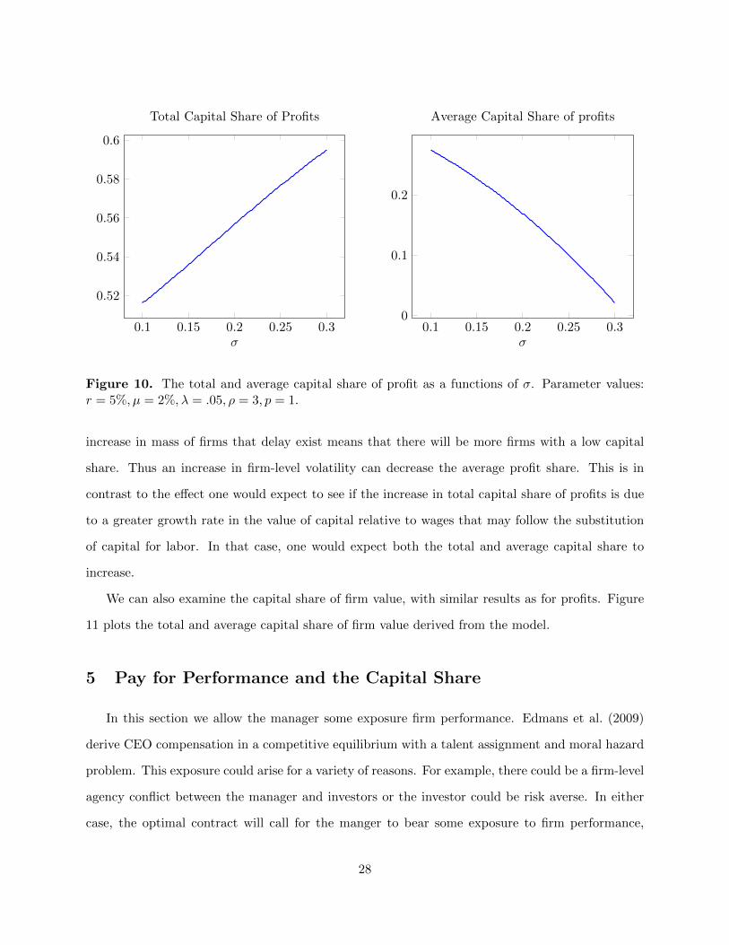
Figure 10 plots a calibrated example. The figure plots the total and average capital share of

profit as a functions of σ. We use the following parameter values: r = 5%, µ = 2%, λ = .05, ρ =

3, p = 1. We can see that the total capital share of profits is increasing in σ while the average capital

share of profits is decreasing. The intuition is as follows. As σ increases, the value of the option

to delay abandonment increases, and hence the optimal threshold at which firms exit decreases.

Holding the total measure of firms fixed, this means that the distribution of profits becomes more

dispersed. The increase in mass of firms in the right tail of the firm size distribution increases the

total profit share, because the profit share measures the ex post profitability of existing firms. This

is effectively a selection bias. The profit share of entering firms is set by setting the NPV of the

investor’s stake in the firm to zero. This NPV calculation integrates over all possible future paths

for firm-level productivity, including those that lead the investor to choose to exit. In contrast,

the stationary distribution of existing firms only consider firms that have survived. Surviving firms

necessarily have a higher capital share of profits, otherwise the investor would have chosen to exit.

Our model also makes a novel prediction about the capital share at the average firm. The

27

0.1 0.15 0.2 0.25 0.3

0.52

0.54

0.56

0.58

0.6

σ

Total Capital Share of Profits

0.1 0.15 0.2 0.25 0.30

0.1

0.2

σ

Average Capital Share of profits

Figure 10. The total and average capital share of profit as a functions of σ. Parameter values:r = 5%, µ = 2%, λ = .05, ρ = 3, p = 1.

increase in mass of firms that delay exist means that there will be more firms with a low capital

share. Thus an increase in firm-level volatility can decrease the average profit share. This is in

contrast to the effect one would expect to see if the increase in total capital share of profits is due

to a greater growth rate in the value of capital relative to wages that may follow the substitution

of capital for labor. In that case, one would expect both the total and average capital share to

increase.

We can also examine the capital share of firm value, with similar results as for profits. Figure

11 plots the total and average capital share of firm value derived from the model.

5 Pay for Performance and the Capital Share

In this section we allow the manager some exposure firm performance. Edmans et al. (2009)

derive CEO compensation in a competitive equilibrium with a talent assignment and moral hazard

problem. This exposure could arise for a variety of reasons. For example, there could be a firm-level

agency conflict between the manager and investors or the investor could be risk averse. In either

case, the optimal contract will call for the manger to bear some exposure to firm performance,

28

0.1 0.15 0.2 0.25 0.3

0.65

0.7

0.75

σ

Total Capital Share of Firm Value

0.1 0.15 0.2 0.25 0.30.43

0.44

0.44

0.44

0.44

σ

Average Capital Share of Firm Value

Figure 11. The total and average capital share of firm value as a functions of σ. Parameter values:r = 5%, µ = 2%, λ = .05, ρ = 3, p = 1.

either for incentive purposes or to improve risk sharing. The precise form of the optimal contract

will depend on the nature of the agency problem or the exact preferences of the managers and

investors. A concern with our results thus far might be that such a sensitivity could mitigate the

insurance nature of the relationship between firms’ owners and their managers, thus decreasing or

reversing the effect of firm level volatility on the capital share of profits. Rather than solve directly

for an optimal contract for a particular problem, we assume that the manager’s contract takes the

following simple affine form

ct = βXt + w. (25)

The sensitivity β of the managers payment ct to the level of productvity is determined by either

the severity of the agency problem or the nature of the risk-sharing problem, and is exogenous from

the standpoint of our model. The fixed wage w is set in equilibrium in the same manner as total

wages are set above. This contract has the advantage of being particularly tractable to analyze in

the context of our model of equilibrium.

29

For a given fixed wage w, the investors problem is

maxτ

[∫ τ

0e−rt((1− β)Xt − w)dt

]. (26)

Again, standard arguments imply that the investor’s value function V (X) must statisfy the following

ODE

(r + λ)V = (1− β)X − w + µXV ′ +1

2σ2X2V ′′, (27)

with the boundary conditions

V (X) = 0, (28)

V ′(X) = 0, (29)

limX→∞

∣∣∣∣V (X)−(

(1− β)X

r + λ− µ− w

r + λ

)∣∣∣∣ = 0. (30)

This problem is essentially the same as one given in equations (5)-(8), up to a scaling of the leading

term by a factor of (1− β). Thus, the solution to equation (27)-(30) is

X =

(1

1− β

)(η

η + 1

)w(r + λ− µ)

r + λ

V (X) =(1− β)X

r + λ− µ− c

r + λ−(

(1− β)X

r + λ− µ− c

r + λ

)(X

X

)−η

where η is defined as above.

Given the solution for the investor’s value, we can apply the investor’s zero ex-ante profit

condition to determine the fixed component of the manager’s equilibrium contract. Doing this

calculation yields

w∗ =

(P (r + λ)(ρ− 1)(ρ− η)

η

(η(r + λ− µ)

(1− β)(η + 1)(r + λ)

)ρ)− 1ρ−1

. (31)

Comparing equations (11) and (31) reveals that the fixed component of the equilibrium affine

30

contract is just the equilibrium wage under full insurance scaled by a function of β. The intuition

here is that we can essentially view the investor’s problem under the affine contract has identically

to the problem under full insurance when the firm’s productivity is scaled by a factor of 1− β.

Now note that the stationary distribution of firm productivity is unaffected by our assumption

of affine contracts, up to a shifting of the optimal abandonment threshold, i.e. the left support of

the stationary distribution. Thus we can again calculate the total capital share of profits in the

stationary distribution to get

Π = 1− (1− β)

(r + λ

r + λ− µ

)(ρ− 1

ρ

)(γ − 1

γ

)(η + 1

η

). (32)

Comparing equations (18) and (32) shows that the total capital share profits under the affine

contract depends on γ and η, and hence on σ, in the same manner as the total capital share

of profits under full insurance. In other words, allowing the manager to share in success of the

successful firms does not change our main results.

6 Economy with Physical Capital and Unskilled Labor

To quantify the effects we describe above, we analyze an extended version of our economy with

physical capital accumulation and unskilled labor.

Again we study an economy populated by a measure of ex ante identical firms. However, now

we will consider firms that require unskilled labor in addition to a manage and that can adjust

the amount of capital under production. A given firm with productivity Xt has a single manager,

capital kt and unskilled labor lt. Total output produced by this firm is given by:

Yt = Xνt F (kt, lt)

1−ν ,

where F is homogeneous of degree one and 0 < ν < 1. Lucas refers to ν as the span of control

parameter of the firm’s manager. Unskilled labor is in fixed supply. We normalize lt = 1. This is

without loss of generality.

31

The firm rents physical capital at a rental rate ρt and unskilled labor at a spot rate wt. The

firm’s gross earnings are given by:

dt(Xt) = Yt − wtlt(Xt)− ρtkt(Xt).

The firm chooses physical capital and unskilled labor to maximize gross earnings. This is a static

optimization problem. We can simply characterize the optimal allocation of physical capital and

labor as a function of the firm’s productivity Xt. To do so, we can define the first moment of X:

Xt =

∫ ∞x

(ex)φt(x)dx.

Given the homogeneity of the production function, it is straightforward to show that physical

capital and unskilled labor are allocated across firms according to the following linear allocation

rule:

kt(Xt) =Xt

Xtkt,

lt(Xt) =Xt

Xtlt,

yt(Xt) =Xt

Xtyt,

where yt = X1−νt F (kt, lt)

ν denotes aggregate output. One can verify that this allocation rule

satisfies the firm’s static first order conditions. As a result, we know that a firm’s gross earnings

are proportional to Xt:

dt(Xt) = (1− ν)yt(Xt) = (1− ν)Xt

Xt

yt.

Thus, we can simplify the investors problem to

V (X; c) = maxτ

E

[∫ τ

0e−rt((1− ν)

Xt

Xt

yt − c)dt], (33)

where V (X; c) is the value of operating a firm with current productivity X given a manager contract

32

c.

The definition of a stationary equilibrium in this economy is the natural extension of the one

given above to a setting in which firms employ unskilled labor and can adjust capital.

Definition 2. A stationary equilibrium consists of a rental rate ρ for physical capital, a wage rate

w, a compensation c for the skilled worker, an exit policy for the shareholder X(·), a stationary

distribution φ, such that, for given (X, y), the exit policy solves the shareholder problem, the

wage rate clears the labor market, the rental rate r clears the market for physical capital, and the

stationary size distribution is consistent with the exit policy X(·).

We focus on a stationary equilibrium in which (Xt, yt) are constant. The solution technique

for the investor’s problem is essentially the same as in the case with constant physical capital and

labor up to a change in the coefficients in the ODE and determination of the optimal abandonment

threshold. For a given candidate equilibrium abandonment threshold X(c), V (X; c) must satisfy

the following ordinary differential equation

(r + λ)V (X; c) = (1− ν)X

Xy − c+ µX

∂

∂XV (X; c) +

1

2σ2X2 ∂2

∂X2V (X; c), (34)

with the boundary conditions

V (X(c); c) = 0, (35)

limX→∞

∣∣∣∣V (X; c)−(

X

r + λ− µ− c

r + λ

)∣∣∣∣ = 0. (36)

Conditions (35) is the standard value matching, while condition (36) arises because as Xt tends to

infinity, abandonment occurs with zero probability as in the simple model we analyzed above.

An important difference between the model with physical capital and unskilled labor and the

simple model given above, is that the abandonment threshold must be consistent with the equilib-

rium distribution of capital and labor. Consider a candidate equilibrium threshold X(c). If all firms

choose to delay abandonment beyond this threshold, average productivity decreases, increasing the

allocation of capital and labor to existing firms with higher productivity. This in turn increases the

33

benefit to delaying abandonment. Whether it is for some abandonment threshold above the mini-

mum level of productivity to obtain in equilibrium depends on how sensitive average productivity

is to the left support of the stationary distribution. For the Pareto distribution we have considered

above, average productivity is very sensitive to the left support of the stationary distribution and

X(c) > Xmin cannot obtain in equilibrium. Thus, the optimal abandonment threshold is given by

X(c) = Xmin (37)

and the solution to equations (34)-(36) is given by

V (X; c) =X

(1− ν)y

X

r + λ− µ− c

r + λ−(

X

(1− ν)y

Xmin

r + λ− µ− c

r + λ

)(X

Xmin

)−η. (38)

where the exponent η is the same as given in the simple model.

Now note that since Xt still has the same dynamics as in the simple model, the form of the

stationary distribution for productivity is unchanged. The only difference is the left support is now

Xmin. It is then possible to calculate the equilibrium average productivity

X =Xminγρ

(γ − 1)(ρ− 1).

Finally, we have assumed that entering firms still draw initial productivity from a Pareto dis-

tribution as in the simple model. Thus, given the solution to the investors value function, it is

straightforward to solve the investors ex ante zero profit condition for the equilibrium c. The

closed form solution for c is somewhat messy and uninformative, so we omit it for brevity.

Once we have solved for the c that sets the NPV to zero, we can back out the actual c, using

(y,X).

6.1 National Income Accounting

Armed with this stationary distribution, we can do national income accounting inside our model.

We use this stationary distribution to calculate the total and average profit share for a range of σ.

34

Specifically, we use the stationary distribution to calculate the aggregate capital share:

Total Capital Share of Rents =

∫∞x ((1− ν) yX e

x − c)φ(x)dx∫∞x (1− ν) yX e

xφ(x)dx

= 1− c

(1− ν)y

Total Capital Share of Output =

∫∞x (ανy + (1− ν) yX e

x − c)φ(x)dx∫∞x (1− ν) yX e

xφ(x)dx

= 1 +αν

1− ν− c

(1− ν)y.

Average Capital Share of Rents = E

[X − cX

]=

∫ ∞x

((1− ν) yX e

x − c(1− ν) yX e

x

)φ(x)dx.

Note, total capital share of out put is equal to total capital share of rents plus a constant that

doesn’t depend on σ, hence the two will have the same comparative static.

In order to make our predictions sharpe, we make some simple assumptions on functional forms.

Specifically we use F (k, l) = kαl1−α. The stand-in agent’s Euler equation for consumption implies

that:

1 + r = (1− τc)(να

y

k− δ)

+ 1.

Atkeson and Kehoe set the capital share ky to 1.46, the corporate tax rate τ to 48.1 percent, δ to

5.5 percent. Hence, the implied να is 19.9 percent. Without loss of generality, we can normalize

the unskilled labor force to one. We also know that we can state total output as:

y = X1−ν1−αν (

k

y)

αν1−αν

35

As a result we can restate the expressions for the factor shares as follows:

Total Capital Share of Rents = 1− c

(1− ν)X1−ν1−αν (ky )

αν1−αν

Total Capital Share of Output = 1 +αν

1− ν− c

(1− ν)X1−ν1−αν (ky )

αν1−αν

.

where k/y is a constant pinned down by the intertemporal Euler equation. We have

Total Capital Share of Output = 1 +αν

1− ν−(

1

1− ν

)(k

y

)− αν1−αν

((ρ− 1

ρ

)(γ − 1

γ

)(1

Xmin

))βc

where

β =1− ν

1− αν.

After some algebra, we can show that

Total Capital Share of Output = α1 − α2

(γ − 1

γ

)(η + 1

η

)+ α3

(γ − 1

γ

)β η + ρ

η(39)

where α1, α2 and α3 are positive constants that don’t depend on σ. The sign of the comparative

static of total capital share of output thus depends on the relative magnitude of κ2 and κ3. When

Xmin is small, κ3 << κ2 and the total capital share of output is increasing in σ

7 Conclusion

We propose a mechanism whereby an increase in firm-level volatility can have important effects

on national income accounting. A firm’s owner insurance it’s manager against firm-level productiv-

ity shocks. As a result, that owner may choose to exit if productivity becomes too low. The level

of the manager’s compensation is set based on expected firm value–which necessarily integrates

36

over paths that end in exit. In contrast, when accounting for income, one typically integrates over

surviving firms which necessarily feature lower capital shares of profit. This leads to an difference

between the aggregate capital share of income, which is calculated ex post, and the capital share of

value at the origination of firm, which is calculated ex ante. When firm-level volatility increases, the

difference can increase, increasing the aggregate capital share and decreasing the average capital

share. We also present time series and cross sectional evidence for Compustat firms consistent with

our proposed mechanism.

37

References

Ai, H., Kiku, D., Li, R., 2013. A mechanism design model of firm dynamics: The case of limitedcommitment. Available at SSRN 2347821.

Ai, H., Li, R., 2015. Investment and CEO compensation under limited commitment. Journal ofFinancial Economics 116 (3), 452 – 472.URL http://www.sciencedirect.com/science/article/pii/S0304405X15000458

Berk, J. B., Walden, J., 2013. Limited capital market participation and human capital risk. Reviewof Asset Pricing Studies 3 (1), 1–37.URL http://raps.oxfordjournals.org/content/3/1/1.abstract

Bloom, N., May 2014. Fluctuations in uncertainty. Journal of Economic Perspectives 28 (2), 153–76.URL http://www.aeaweb.org/articles?id=10.1257/jep.28.2.153

Campbell, J. Y., Lettau, M., Malkiel, B. G., Xu, Y., 2001. Have individual stocks become morevolatile? an empirical exploration of idiosyncratic risk. The Journal of Finance 56 (1), 1–43.URL http://dx.doi.org/10.1111/0022-1082.00318

Comin, D., Philippon, T., 2005. The rise in firm-level volatility: Causes and consequences. NBERMacroeconomics Annual.

Dixit, A. K., Pindyck, R. S., 1994. Investment under uncertainty. Princeton university press.

Doidge, C., Karolyi, G. A., Stulz, R. M., May 2015. The u.s. listing gap. Working Paper 21181,National Bureau of Economic Research.URL http://www.nber.org/papers/w21181

Donangelo, A., Gourio, F., Palacios, M., 2015. Labor share and the value premium. Tech. rep.

Edmans, A., Gabaix, X., Landier, A., 2009. A multiplicative model of optimal ceo incentives inmarket equilibrium. Review of Financial Studies 22 (12), 4881–4917.URL http://rfs.oxfordjournals.org/content/22/12/4881.abstract

Fama, E. F., French, K. R., 2004. New lists: Fundamentals and survival rates. Journal of FinancialEconomics 73 (2), 229 – 269.URL http://www.sciencedirect.com/science/article/pii/S0304405X04000315

Gabaix, X., 2011. The granular origins of aggregate fluctuations. Econometrica 79 (3), 733–772.URL http://dx.doi.org/10.3982/ECTA8769

Gabaix, X., Landier, A., 2008. Why has ceo pay increased so much? The Quarterly Journal ofEconomics 123 (1), 49–100.URL http://qje.oxfordjournals.org/content/123/1/49.abstract

Herskovic, B., Kelly, B. T., Lustig, H. N., Van Nieuwerburgh, S., 2015. The common factor inidiosyncratic volatility: Quantitative asset pricing implications. Journal of Financial Economics.

38

Holmstrom, B., Milgrom, P., 1991. Multitask principal-agent analyses: Incentive contracts, assetownership, and job design. Journal of Law, Economics, & Organization 7, 24–52.URL http://www.jstor.org/stable/764957

Hopenhayn, H., 2002. Exit, selection, and the value of firms. Journal of Economic Dynamics andControl 16(3-4), Pages 621–653.

Hopenhayn, H. A., 1992. Entry, exit, and firm dynamics in long run equilibrium. Econometrica60 (5), 1127–1150.URL http://www.jstor.org/stable/2951541

Jovanovic, B., 1982. Selection and the evolution of industry. Econometrica 50 (3), 649–670.URL http://www.jstor.org/stable/1912606

Karabarbounis, L., Neiman, B., 2013. The global decline of the labor share. Tech. rep., NationalBureau of Economic Research.

Kocherlakota, N., 1996. Implications of efficient risk sharing without commitment. Review of Eco-nomic Studies 63, 595–610.

Leland, H. E., 1994. Corporate debt value, bond covenants, and optimal capital structure. TheJournal of Finance 49 (4), 1213–1252.URL http://dx.doi.org/10.1111/j.1540-6261.1994.tb02452.x

Loughran, T., Ritter, J. R., 1995. The new issues puzzle. The Journal of Finance 50 (1), 23–51.URL http://dx.doi.org/10.1111/j.1540-6261.1995.tb05166.x

Lustig, H., Syverson, C., Nieuwerburgh, S. V., 2011. Technological change and the growing inequal-ity in managerial compensation. Journal of Financial Economics 99 (3), 601 – 627.URL http://www.sciencedirect.com/science/article/pii/S0304405X10002199

Luttmer, E. G., 2012. Technology diffusion and growth. Journal of Economic Theory 147 (2), 602– 622, issue in honor of David Cass.URL http://www.sciencedirect.com/science/article/pii/S0022053111000196

Luttmer, E. G. J., 2007. Selection, growth, and the size distribution of firms. The Quarterly Journalof Economics 122 (3), 1103–1144.URL http://www.jstor.org/stable/25098869

Perla, J., Tonetti, C., Benhabib, J., et al., 2014. The growth dynamics of innovation, diffusion, andthe technology frontier. In: 2014 Meeting Papers. No. 818. Society for Economic Dynamics.

Piketty, T., Zucman, G., 2014. Capital is back: Wealth-income ratios in rich countries, 1700-2010.The Quarterly Journal of Economics.URL http://qje.oxfordjournals.org/content/early/2014/05/21/qje.qju018.abstract

Song, J., Price, D. J., Guvenen, F., Bloom, N., von Wachter, T., May 2015. Firming up inequality.Working Paper 21199, National Bureau of Economic Research.URL http://www.nber.org/papers/w21199

39

Thomas, J., Worall, T., 1988. Self-enforcing wage contracts. Review of Economic Studies 15, 541–554.

Zhang, M. X., 2014. Who bears firm-level risk? implications for cash flow volatility, working PaperU.T. Austin.

A Proofs

A.1 Derivation of equilibrium compensation

The equilibrium wage is given by the solution to the following equation

∫ ∞X(c)

V (X; c)f(X)dX = P

where X(c) is given by equation (9) and V (X; c) is given by equation (10). Note that this equation

is equivalent to condition 3 of Definition 1. First evaluate the integral on the left hand side we have

∫ ∞X(c)

(X

r + λ− µ− c

r + λ−(

X(c)

r + λ− µ− c

r + λ

)(X

X(c)

)−η) ρ

X1+ρdX

=(ρX(c))ρ(

X(c)

(r + λ− µ)(ρ− 1)+

c

(r + λ)ρ+X(c)(r + λ)− c(r + λ− µ)

(r + λ− µ)(r + λ)(η + ρ)

)=

(η(r + λ− µ)

(1 + η)(r + λ)

)−ρ( η

(r + λ)(ρ− 1)(η + ρ)

)c−(ρ−1).

Note that our assumption on the Pareto form f(X) facilitates that computation of the integral

above because both V (X; c) and f(X) are power functions. This integral represent the expected

value of the firm to the shareholder after paying the fixed cost but before realizing the initial

productivity of the firm. Since ρ > 1, it is monotonically increasing in c, and we can solve to get

the expression for equilibrium compensation given in (11).

A.2 Derivation of stationary distribution

The ODE for φ(x) has the following general solution

φ(x) = A1eγ1x +A2e

−γ2x +A3e−ρx (40)

40

where γ1 and γ2 are given by:

γ1 =µ− 1

2σ2 +

√(µ− 1

2σ2)2 + 2σ2λ

σ2(41)

γ2 =−(µ− 1

2σ2) +

√(µ− 1

2σ2)2 + 2σ2λ

σ2(42)

First note that γ1 > 0 implies A1 = 0. To ease notation we drop the subscript on γ2. Next note

that an application of the ODE gives

A3 = − ρψ12ρ

2σ2 + ρ(µ− 12σ

2)− λ. (43)

Finally, the boundary condition implies that

A2e−γx +A3e

−ρx = 0

so

A2 = −A3e(γ−ρ)x. (44)

The result in equation (15) directly follows from the above and an application of the market clearing

condition for managers.

A.3 Derivation of Total and Average Capital Share of Profits.

We have

Π =

∫∞x (ex − c)φ(x)dx∫∞

x exφ(x)dx= 1−

c∫∞x φ(x)dx∫∞

x exφ(x)dx

= 1− c∫∞x exφ(x)dx

41

where the second step follows from the market clearing condition given in equation (14). To continue

the calculation we have

∫ ∞x

exφ(x)dx =

∫ ∞x

ργ

ρ− γ

(e−(γ−1)x+γx − e−(ρ−1)x+ρx

)dx

= X

(ρ

ρ− 1

)(γ

γ − 1

)=

(ρ

ρ− 1

)(γ

γ − 1

)(η

η + 1

)(r + λ− µr + λ

)c

Substituting this expression into the expression for Π given above yields the desired result. The

derivation of the average capital share is similar.

B Data Appendix

BLS Data: BEA develops employee compensation data as part of the national income accounts.

These quarterly data include direct payments to labor, wage and salary accruals (including execu-

tive compensation), commissions, tips, bonuses, and payments in kind representing income to the

recipients and supplements to these direct payments. Supplements consist of employer contribu-

tions to funds for social insurance, private pension and health and welfare plans, compensation for

injuries, etc.

The compensation measures taken from establishment payrolls refer exclusively to wage and

salary workers. Labor cost would be seriously understated by this measure of employee compensa-

tion alone in sectors such as farm and retail trade, where hours at work by proprietors represent

a substantial portion of total labor input. BLS, therefore, imputes a compensation cost for labor

services of proprietors and includes the hours of unpaid family workers in the hours of all employees

engaged in a sector. Labor compensation per hour for proprietors is assumed to be the same as that

of the average employee in that sector for measures found in the BLS news release, “Productivity

and Costs”.

42

Figure 12. Average and Aggregate Factor Share of Output – Volatility Sectors

1960 1970 1980 1990 2000 20100.1

0.12

0.14

0.16

0.18

0.2

0.22

0.24

0.26

Ave

rag

e

0.12

0.13

0.14

0.15

0.16

0.17

0.18

0.19

0.2

Ag

gre

gate

Low σ(r) Group

Average Trend

Aggregate Trend

1960 1970 1980 1990 2000 2010-2

-1

0

1

Avera

ge

-0.2

0

0.2

0.4

Aggre

gate

High σ(r) Group

(a) OIBDP/Sales

1960 1970 1980 1990 2000 20100.22

0.24

0.26

0.28

0.3

Avera

ge

0.05

0.1

0.15

0.2

0.25

Aggre

gate

Low σ(r) Group

Average Trend

Aggregate Trend

1960 1970 1980 1990 2000 20100.2

0.3

0.4

0.5

0.6

0.7

0.8

Avera

ge

0.1

0.15

0.2

0.25

0.3

0.35

0.4

Aggre

gate

High σ(r) Group

(b) Extended XLR/Sales

The plots present the time series of factor share of output for low and high volatility groups. Panel(a) shows the average and aggregate time series of operating income (OIBDP) to sales ratio. Panel(b) shows the average and aggregate time series of extended labor cost (XLR) to sales ratio. Forboth (a) and (b), we classify firms into three groups (low, median, high) based on the idiosyncraticreturn volatility. The plots show data moments of the lowest and highest volatility groups. Source:Compustat Fundamentals Annual (1960-2014).

43

Figure 13. Average Capital Share of Output – Volatility Sectors

1960 1970 1980 1990 2000 2010

Year

-0.1

-0.05

0

0.05

0.1

0.15

0.2

0.25

0.3

Ave

rag

e O

IBD

P/S

AL

ES

Low σ (r) Sector

Assets <20%

20% < Assets 40%

40% < Assets < 60%

60% < Assets < 80%

Assets > 80%

1960 1970 1980 1990 2000 2010

Year

-3.5

-3

-2.5

-2

-1.5

-1

-0.5

0

0.5

Ave

rag

e O

IBD

P/S

AL

ES

High σ (r) Sector

Assets <20%

20% < Assets 40%

40% < Assets < 60%

60% < Assets < 80%

Assets > 80%

The plots present the average capital share of output within each size quintile for both high and lowvolatility sectors. Size is measured by total assets, and the capital share is measured as operatingincome (OIBDP) divided by sales (SALE). Source: Compustat Fundamentals Annual (1960-2014).

44

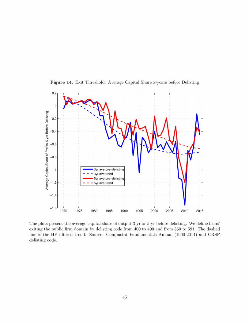
Figure 14. Exit Threshold: Average Capital Share x-years before Delisting

1970 1975 1980 1985 1990 1995 2000 2005 2010 2015−1.6

−1.4

−1.2

−1

−0.8

−0.6

−0.4

−0.2

0

0.2

Avera

ge C

apital S

hare

of P

rofits

X y

rs B

efo

re D

elis

ting

3yr ave pre−delisting

3yr ave trend

5yr ave pre−delisting

5yr ave trend

The plots present the average capital share of output 3-yr or 5-yr before delisting. We define firms’exiting the public firm domain by delisting code from 400 to 490 and from 550 to 591. The dashedline is the HP filtered trend. Source: Compustat Fundamentals Annual (1960-2014) and CRSPdelisting code.

45

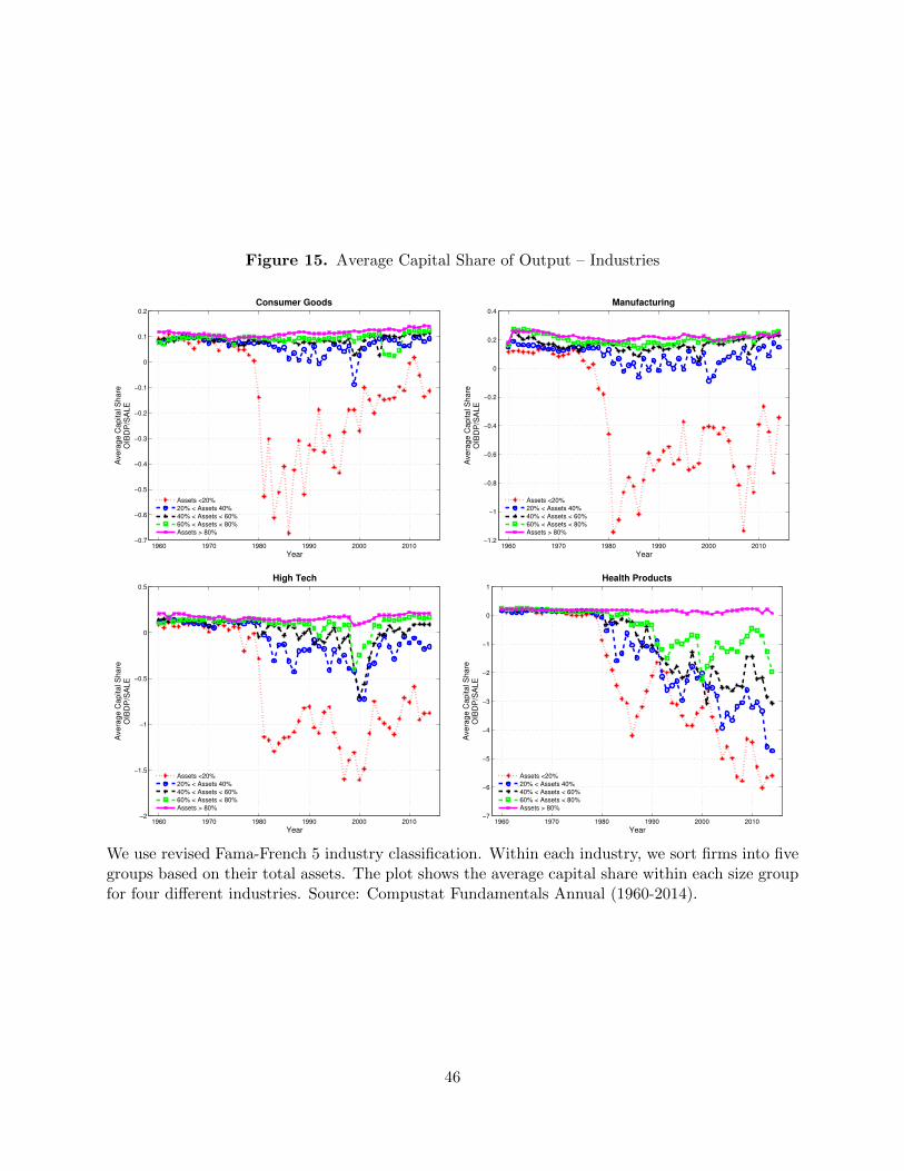
Figure 15. Average Capital Share of Output – Industries

1960 1970 1980 1990 2000 2010−0.7

−0.6

−0.5

−0.4

−0.3

−0.2

−0.1

0

0.1

0.2

Avera

ge C

apital S

hare

OIB

DP

/SA

LE

Year

Consumer Goods

Assets <20%

20% < Assets 40%

40% < Assets < 60%

60% < Assets < 80%

Assets > 80%

1960 1970 1980 1990 2000 2010−1.2

−1

−0.8

−0.6

−0.4

−0.2

0

0.2

0.4

Avera

ge C

apital S

hare

OIB

DP

/SA

LE

Year

Manufacturing

Assets <20%

20% < Assets 40%

40% < Assets < 60%

60% < Assets < 80%

Assets > 80%

1960 1970 1980 1990 2000 2010−2

−1.5

−1

−0.5

0

0.5

Avera

ge C

apital S

hare

OIB

DP

/SA

LE

Year

High Tech

Assets <20%

20% < Assets 40%

40% < Assets < 60%

60% < Assets < 80%

Assets > 80%

1960 1970 1980 1990 2000 2010−7

−6

−5

−4

−3

−2

−1

0

1

Avera

ge C

apital S

hare

OIB

DP

/SA

LE

Year

Health Products

Assets <20%

20% < Assets 40%

40% < Assets < 60%

60% < Assets < 80%

Assets > 80%

We use revised Fama-French 5 industry classification. Within each industry, we sort firms into fivegroups based on their total assets. The plot shows the average capital share within each size groupfor four different industries. Source: Compustat Fundamentals Annual (1960-2014).

46