NASA Contractor Report 3493

Turbofan Forced Mixer-Nozzle Internal Flowfield II - Computational Fluid Dynamic Predictions

M. J. Werle and V. N. Vatsa

CONTRACT NAS3-20951 APRIL 1982

NASA

https://ntrs.nasa.gov/search.jsp?R=19820014585 2018-07-14T05:09:33+00:00Z

NASA Contractor Report 3493

TECH LIBRARY KAFB, NM

llnlllllRNllNlllRlDllllrlllll 0062253

Turbofan Forced Mixer-Nozzle Internal Flowfield II - Computational Fluid Dynamic Predictions

M. J. Werle and V. N. Vatsa United Techno Zogies Research Center East Hartford, Connecticut

Prepared for Lewis Research Center under Contract NAS3-2095 1

National Aeronautics and Space Administration

Scientific and Technical Information Branch

1982

TABLE OF CONTENTS

ABSTRACT ..................................

TABLEOFCONTENTS .............................

I. INTRODUCTION .............................

II. ANALYTICAL/NUMERICAL APPROACH .....................

1. General Statement ......................... 2. Pre-analysis Element ....................... 3. Mixer Flow Element ........................ 4. Output Element ..........................

III. RESULTS AND DISCUSSION ........................

1. 2. 3. 4.

5.

General Statement . . . . ..................... 5 Hot Jet Mixing . . . . . ..................... 5 Diffuser Flow . . . . . . ..................... 6 Mixer Nozzle Flow - Cold ..................... 7

(a) General Description ..................... 7 (b) Input Profiles . . ..................... 8 (c) Downstream Profiles ..................... 10

Mixer Nozzle Flow - Hot . . . . . . . . . . . . . . . . . . . . . . 12

(a) General Description ..................... 12 (b) Input Profiles . . ..................... 12 (c) Downstream Profiles ..................... 13

IV. CONCLUSIONS ..............................

V. REFERENCES ..............................

APPENDIX A - USER'S MANUAL -UTRCMIXERCODE ................

APPENDIXB - PRATT AND WJJITNEY AIRCRAFT MIXER NOZZLE FLOW ANALYSIS .....

i

ii

1

2

5

16

17

64

68

iii

I. INTRODUCTION

In an effort to increase the efficiency of turbofan engines, the concept of forced mixing of engine core and fan exhaust gases has been introduced. Studies to date (see Ref. 1 for example) indicate a potential for significant Improvement in engine performance through this simple modification to an engine exhaust system. To better guide the design of such systems though, a reliable analytical means is required for predicting the degree of thermal mixing that takes place Inside the engine exhaust duct aft of the mixer lobes. This flow involves a highly three dimensional mixing of a hot engine core flow with a cold fan flow as it accelerates from a subsonic level at the engine exhaust to a sonic state at the nozzle exit plane. As such It is anticipated that the prediction of such a complex flow process could only be accomplished using advanced computational fluid dynamic concepts.

The overall goal of the current study was to develop and assess a computer code to analyze the mixing between the fan and core flows in this turbofan "mixing duct". To accomplish this, the overall effort was conducted in three major subelements - the first being a benchmark experimental study to provide a basis of assessment (see Vol. 1 of this report), the second being the de- velopment of a computer code for solving the mixing flow equations in an axi- symmetric duct (see Vol. 3 of this report), and the third the development of a preprocessor element and overall assessment of the codes' capabilities. The details of this last program element are presented in the current report.

The principal tasks conducted in the current program element were: 1) development of the total analytical program including the SRA mixing analysis (Vol. 3); 2) evaluation of the basic turbulence model through comparison with experimental data; 3) assessment of the final Mixer Code predictions with the benchmark data presented indetailin Vol. 1 of this report.

The overall results achieved indicate that the current code gives reasonable qualitative predictions of the flow processes in the low subsonic regions of a mixer nozzle but underpredicts the thermal mixing in the highly accelerated flow regions approaching the nozzle exit for the low bypass type configuration tested here.

During this study, Mr. G. F. Kardas and Dr. W. Presz, of Pratt and Whitney Aircraft Group - Commercial Products Division, East Hartford, Connecticut, acted in a consulting and advisory role to UTRC, provided the forced mixer model hardware employed in the experimental program, and assisted in the engineering evaluation of the flowfield predictions gen- erated by the computational code. In addition, they performed the turbofan forced mixer nozzle analysis presented in Appendix B of this report.

II. ANALYTICAL/NUMERICAL APPROACH

1. General Statement

The general computer code produced and assessed here contained three major elements: a Pre-analysis Element concerned with coordinate generation and input data processing; a Mixer Flow Element concerned with predicting the detailed mixing of the core and fan flows; and an Output Element con- cerned with post processing and analysis of the computed results. Each such element is described in detail below.

2. Pre-analysis Element

The first major task of the mixer code involves generation of an orthogonal coordinate system for the calculation scheme. This is accomplished using Anderson's (Ref. 2) ADD code approach wherein a conformal mapping is employed to generate an orthogonal net within the duct geometry of interest. This "2-D" net is then rotated about the axis of symmetry to produce the full coordinate system within the mixer nozzle (see Fig. l(a)).

Once the coordinate system is fixed it is only necessary to establish the initial plane data that is to be used as input to the second code element, the Mixing Flow Element. For the current applications* it is assumed that the flow at the exit of the mixer lobes (see Fig. 1) has been defined by some inde- pendent process, either experimental or analytical, and that the full velocity, temperature, and pressure field is defined at a finite number of points on some plane - plane I of Fig. 1. This plane need not, and in general will not, correspond to a coordinate plane nor will the data points correspond to the coordinate grid points discussed above. Thus a preprocessing procedure is followed for extrapolating and interpolating the initial plane data-base to the inlet coordinate plane and grid. To do this, the coordinate values of the inlet data point locations are first found using a simple look-up and interpolation routine. Once these are established, a particular coordinate plane is identified as the "inlet" station by seeking that coordinate plane with the minimum longitudinal coordinate distance from the data plane. All data points on the initial data plane were moved without change to the inlet plane along longitudinal coordinate lines. This procedure is based on the assumption that these coordinate lines approximate streamlines, and that the fluid properties will experience small variation over short distances. Once the initial data-base has been moved to the initial plane and velocity components resolved into the coordinate directions, simple linear inter- polations are used between points to establish values at the usually denser coordinate grid locations. A final check is made to verify that these inter- polations and extrapolations capture the details of the phenomenon such as

* The mixer code has the option to construct its own Starting Profiles for given velocity and temperature distributions along a coordinate line of Fig. 1.

2

shear layers, etc. and modifications made where necessary to ensure a valid representation of the inlet flow state.

3. Mixer Flow Element

This code element is concerned solely with the numerical solution of the governing equations in the axisymmetric nozzle with a three-dimensional inlet flow as defined above. The particular code element employed here was developed by Kreskovsky, et al. (see Ref. 3) as part of the current effort. The details of the solution element are presented in Vol 3 (Ref. 3) of this report and will not be repeated here. The principal features of that code are that it employs a subset of the initial plane data to start an implicit finite difference solution scheme that marches in a single pass through the mixer nozzle to the exit plane. For the current application, all wall boundary layer effects were considered of secondary importance. While the general code does contain a two equation turbulence model, it was not employed here for the mixer calculation. Rather, a simpler, wake-like eddy viscosity model defined in detail in Vol. 3 of this report has been used throughout. One other major aspect of the current code concerns its use of an approximate representation of compressibility influences on the pressure field imposed on the viscous mixing evaluation. In the SRA mixer nozzle code the longitudinal pressure gradient field was approximated using an incompressible potential flow solution, thereafter adjusted with a modified Prandtl-Glauert type correction.

4. Output Element

Once the mixer nozzle calculations have been completed, two principal activities take place in an output element. The first involves a simple movement of the computed results to a more convenient output plane to facili- tate comparison with other results - either experimental or analytical. This

process is a direct reversal of that used in the Pre-analysis Element and Involves simple interpolation and extrapolation to obtain the computed results on some convenient plane.

The second activity In the Output Element involves the calculation of general performance parameters for the overall mixer nozzle. In this regard four principal parameters as defined below are calculated from the detailed flow field predictions (see Ref. 3 for a discussion of the first three of these).

3

1.) Mass Averaged Total Pressure Loss:

J 2( 'Tref'PTI -

A (dJz)=f piidA

c = PT

/ pi.dA

A

2.) Ideal Thrust Coefficient:

T/TI = lypM2dAfl YpM'dA

3.) Area Averaged Mach Number:

M=

4.) Total Temperature Mixing

(1)

(2)

(3)

(4)

where TT is the mass averaged total temcerature.

4 \

III. RESULTS AND DISCDSSION

1. General Statement

The general mixer code described above has been applied here to four principal test cases for each of which detailed experimental data was avail- able for direct code assessment. The four test cases were: (1) a hot, free- jet mixing problem used to compare and assess the wake and T.K.E. turbulence models; (2) a diffuser duct flow used to assess the wall boundary layer pre- dictions; (3) a cold flow mixer configuration used to assess the pressure mixing; and (4) a hot flow mixer configuration used to assess the thermal mixing prediction.

2. Hot Jet Mixing

Application of the basic mixer code of Kreskovsky et al. (Ref. 3) to a cold coflowing jet mixing problem has been presented in detail in Vol. 3 of, this report showing excellent comparison with experimental data. The results presented here focus only on the application of the current code to a case with a temperature variation from the jet to outer stream state typical of that encountered in mixer applications. In essence, this represents a de- generate forced mixer configuration in which the lobe geometries are of unit height and the fan flow is at zero velocity. The actual case studied here was that of Heck presented as Test Case 8 in the NASA summary of data on free turbulent shear flows (Ref. 4). Although some question exists about the accuracy of the data, it represents the only such case available at this time. The flow configuration was that ,of a 10.16 cm (4 inch) diameter jet at a Mach number of 0.2 and temperature of 889OK (1600'~) exiting'into a 1.22 m (4 ft) diameter test section at an ambient state. The calculations were initiated at a measurement station 0.85 m (2.79 ft) aft of the jet exit plane. Here the measured values of the jet core velocity and temperature, as well as the shear layer width, were used to construct initial plane profiles (see Ref. 3) as shown in Figs. 2(a) and 2(b). Note that for this case, a small artificial free stream velocity was imparted to the computed flow results to avoid flow entrainment complications at the outer boundary. The jet version of the SRA mixer code was originally constructed for application to confined jet flow and, as such, does not account for mass entrainment at the outer boundary. Application of this approach to the free jet data of Ref. 4 thus requires construction of an artificial velocity along the outer jet boundary to approximate entrainment effects. For the current case, it was found that an outer velocity level of 5% of the jet exit value well approximated the experimental results.

5

Profiles were constructed on a lateral grid space according to a hyperbolic grid stretching scheme in order to capture the large gradients of the shear layer. The resulting starting profiles are presented in Fig. 2(a) and (b) and are seen to give a reasonable quantitative representation of the measured flow conditions - which then display uncertainty in the centerline temperature levels of Fig. 2(b).

The mixer code was applied to this case using simple inviscid like boundary conditions at the outer shroud (zero normal velocity) with solutions marched from the initialization plane to a distance of 1.7 m (5.58 ft) using the T.K.E. turbulence model. Comparisons with the measured axial velocities and total temperatures are presented in Figs. 2(a) and (b) where it is seen that the current results match the observed centerline region velocity and temperature decay trends. The observed spreading of the velocity field is also predicted reasonably well in Fig. 2(a) although the use of an artificial slip velocity at the edge makes direct quantitative assessment somewhat difficult. Similarly, as shown in Fig. 2(b) the temperature mixing trends of the data are predicted by the code but the detailed temperature levels are underpredicted.

3. Diffuser Flow

The test case considered here corresponded exactly to the experimental study of Frazer (Ref. 5). The configuration corresponded to a 0.15 m (0.5 ft) dia straight pipe with cold flow at U = 51.52 m/set (169 ft/sec) into a coni- cal diffuser with a half angle of 10'. This case has been studied by numerous previous investigators (see Ref. 6, for example) as a means of assessing the accuracy of viscous wall effect predictions. Calculations were performed here with both the wake and TKR turbulence models and with two lateral grid spacings. The first grid was obtained from the conformal mapping approach discussed in Section II above as applied to a constant lateral grid spacing of 5% of the duct radius and a longitudinal step of 2% of the duct radius. Since this grid is too coarse to represent the local gradients in the boundary layer region, a second grid was constructed with a packing of the lateral grid mesh points in the wall boundary layer regions. For this case the lateral grid was again constructed with 20 mesh points, except that here a Roberts transformation (see Ref. 7) was used to vary the mesh width.

Solutions for this configuration were initiated at a station 2 diameters upstream of the diffuser. For this process, the experimental data (see Ref. 5) were employed to construct Inlet axial velocities and an average static pres- sure of Pavg = 0.1 atm. Solutions were obtained downstream of the initial station first with the uniform lateral grid spacing and both the eddy viscosity and TKR turbulence models. The resulting centerline velocity, surface skin

6

friction, and surface pressure coefficient distributions are presented in Figs. 3(a), (b), and (c), respectively. Not surprisingly these results show that the turbulence model has virtually no effect on the inviscid nature of the flow - i.e., the centerline velocity (Fig. 3(a)) or pressure (Fig. 3(b)). The boundary layer representation itself is only slightly influenced as shown in the skin friction comparisons of Fig. 3(c). Comparisons with experimental data were found to markedly improve as the grid resolution of the wall boundary layer region was increased. As shown in Figs. 3(a) through 3(c), all flow properties predictions improve with this change - the most notable improvement being for the skin friction (Fig. 3(c)). The slight changes in centerline velocity (Fig. 3(a)) and pressure levels (Fig. 3(b)) are apparently due to an improved estimate of the boundary layer displacement induced blockage in the diffuser as the boundary layer thickens in its approach to separation at x = 0.61 m (2 ft), see Fig. 3(c).

4. Mixer Nozzle Flow - Cold

(a) General Description ------- --

Solutions have been obtained for the flow in an axisymmetric nozzle downstream of the lobe mixer configuration depicted in Figs. la and lb.* Figure la shows the overall nozzle/centerbody geometry and position of the lobe mixers between the upper fan flow and lower engine flow. An end view sketch of the lobe geometries is shown in Fig. lb. For the cases studied here, both streams were held at an ambient stagnation temperature of 289'K (520'R) with a nominal engine flow stagnation pressure of 261 kN/M2 (5460 lbf/ ft2) and a fan stagnation pressure of 240 kN/M2 (5021 lbf/ft2>.

The computational grid employed for the current calculation was obtained from the conformal mapping routine described in Section II-2 above. For this purpose, three adjustments were made, first the annular nozzle contour was extended upstream to the initial point of Fig. la, second, the plug center- body was faired smoothly into the centerline to avoid separation in the cal- culation, and third, the nozzle contour was continued downstream as shown to provide smooth coordinate contours at the nozzle exit plane. A general grid was then generated using 20 evenly spaced points across the flow path, 100 grid points evenly spaced longitudinally, and 9 azimuthal grid points spaced uniformly over 15O of arc (see Fig. lb). The viscous flow calculations were performed on a subset of this grid. This subgrid extended essentially from the inlet station "I" to the exit station "e" using 26 longitudinal grid stations strategically chosen to capture regions of high gradients.

*Detail specifications on the test hardware are presented in Vol. 1 of this report.

7

(b) input Profiles -----

Input profiles for the numerical solutions were established from experimental measurements (see Ref. 8) taken at Station I. This was accomplished using simple linear extrapolations between measurement points to set the values at grid nodal points. Also, an approximation was made to set initial conditions along a lateral grid line based on values dis- tributed along the vertical measurement line (see Fig. la). For this purpose, all flow properties were assumed to hold constant along stream- lines over the short distance between the initial measurement plane I and the calculation initiation plane (see Fig. la). Here the streamline locations were taken to be approximately those used for the coordinate system construc- tion of Fig. la.

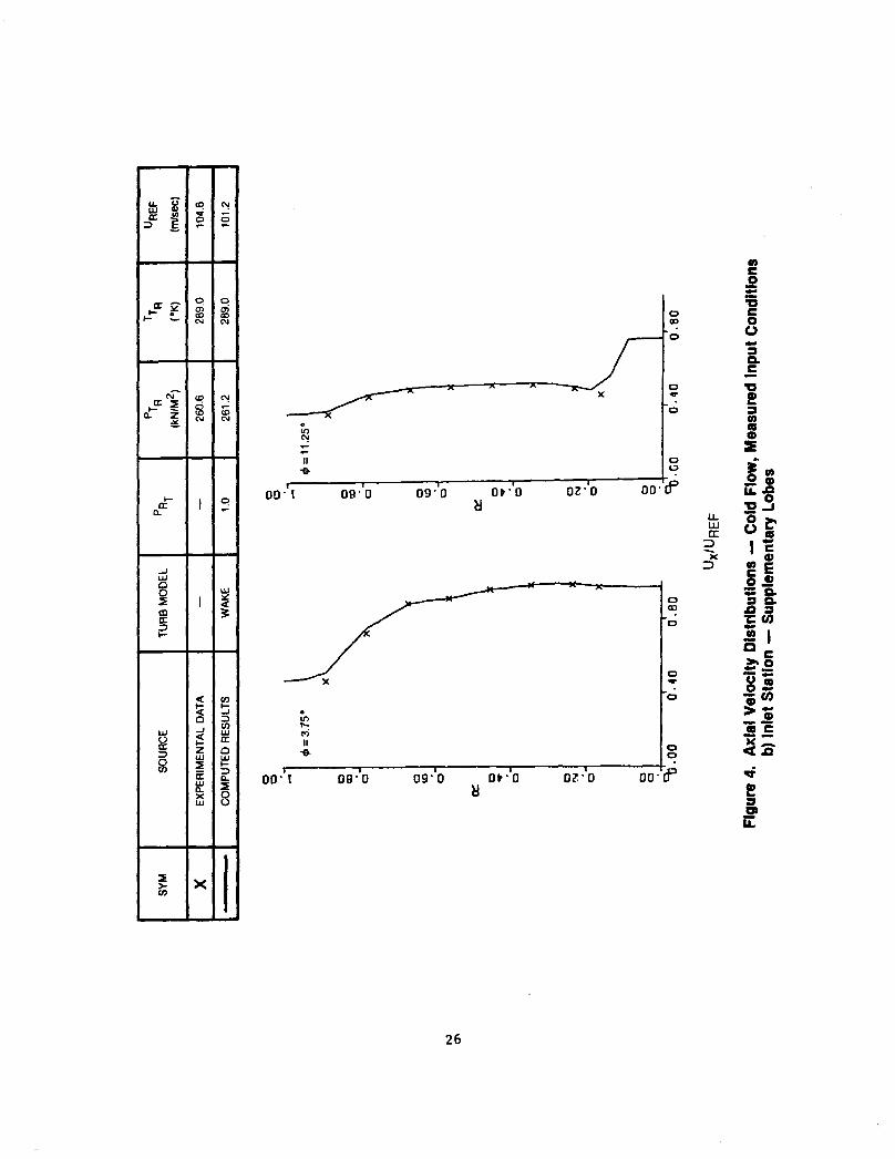
Typical results from this initial data preprocessing procedure are given for the longitudinal velocity in Figs. 4(a) and (b) showing the actual ex- perimental data and curve fitted analytical distributions used as code input. Note that the radial coordinate position has been normalized to vary from zero to unity for all positions through the definition

R= r-rmin (5) r -r

UELX min

while the velocity has been normalized with a reference value defined as the core velocity value at the inlet station and #I = O", R = 0.2. The resulting velocity distributions are shown in Figs. 4(a) and (b) to very accurately represent the experimentally measured profiles. Note that these profiles have been adjusted at the $I = 11.25' and 15' locations to estimate the engine core velocities under the lobes where no velocities are measured. To do this, the densely measured total pressure profiles in this region (see Figs. 7(a) and (b)) were used to calculate the velocity under the assumption of a constant static pressure level over this portion of the flow field. A final adjustment was made to the input velocity profiles to set the flow choking condition at the nozzle exit station. It was found in the initial phases of this study that a sonic Mach number was predicted to occur along the outer casing wall region ahead of the nozzle exit plane. This was believed to be directly related to the lack of boundary layer resolution on the shroud and plug flow. The diffuser flow analysis discussed in Section III-3 above clearly indicated the need to provide a fine grid resolution near the walls in order to properly represent blockage effects in such internal flows. As in the diffuser flow case, it was found that inclusion of the boundary layer option in the SRA code using a coarse grid near the walls did not improve the com- parisions with the data. It was decided here not to redistribute and pack the mesh points near the wall (as was done for the diffuser case) because

this would have caused a lack of resolution of the critical mixing process taking place around the mixer lobes.* Thus an adjustment was made to the reference velocity level to uniformly reduce the input mass flow - in effect to distribute the boundary layer mass defect over the entire inlet plane. As indicated in the table of Fig. 4(a), the computational results were obtained with the reference velocity reduced 3X from the experimental value - resulting in the shroud sonic point exit plane Mach number profile shown in Fig. 8. This was found to be a crucial step in the calculation procedure - producing as much as a 15% reduction of the predicted exit Plane Centerline velocity levels. The resulting compariaono with experimentaI data given below will clearly support the validity of thia approach. The one difficulty that la encountered in use of this approach is the iterative aspect it introduces into the solution procedure since the inlet velocity levels must be set to achieve a sonic condition at the nozzle exit. It was found here that use of a simple one-dimensional approach provided a very effective means of setting the inlet plane adjustment level. An initial run was made with the measured level of reference velocity and note made of the Mach number at the exit plane ahroud location. The inlet plane reference velocity was then modified according to the one-dimensional isentropic relations to produce a maximum exit plane Mach number of unity.

The procedure discussed above was also used to establish the input profiles of the radial and azimuthal velocities as depicted in Figs. S(a), (b) and 6(a), (b) - again adjustments being made near the hub to more accurately represent the engine velocities. It is important to note that the analytical inlet profiles used by the code are not precise curve fits to the data. Once the data has been curve fitted and read into t!he code, a preprocessing occurs that provide an approximate balance of the conservation laws at the initial plane. In this process the secondary velocity field is adjusted to the levels shown in Figs. 5(a), (b), 6(a) and 6(b).

Note that the radial velocity profiles (Fig. S(a), (b)) clearly show the strong lobe induced inflow from the fan and outflow of the engine gas. These velocity levels were found to play the dominant role In the mixing process of the two streams, as they introduce very significant levels of secondary flow vorticity and subsequent convective mixing of the two streams.

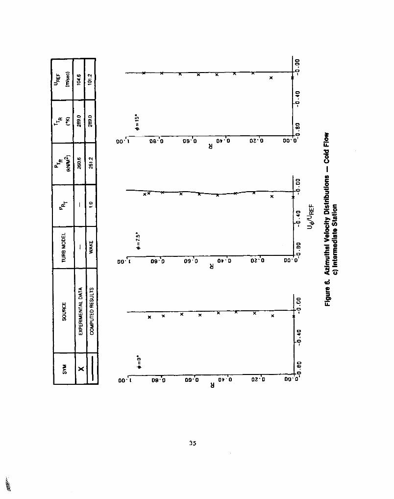
The azimuthal velocity levels shown in Figs. 6(a), (b) were found to be quite small in the inlet plate for R > 0.18. Here the data was found to indi- cate a slight amount of azimuthal velocity both at 4 - 0' and 15'. indicating a small amount of swirl In the inlet flow - apparently traceable to the inlet guide vanes upstream of the lobe mixer region (see Vol. I). Swirl could be present for values of R < 0.18 and could contribute to the mixing process. No attempt was made to account for this effect in the present study which was con- ducted with the assumption that the flow is azimuthally periodic Over all lobes of the inlet plane. The azimuthal velocities at the remaining locations 0 = 3.75, 7.5 and 11.25 show a very slight but distinct clockvise rotation of

* Subsequent work at NASA Lewis Research Center has updimensioned the code to allow denser meshing.

9

theflowas the hot core flow crosses at the low R values over into the colder fan flow. This effect Is better represented in Fig. 6(b) and discussed at length in Ref. 8. The code inlet profiles seem to represent this aspect of the flow quite accurately.

As discussed in Section II, the SRA mixer code also requires as input the average static pressure levels measured over the input plane. This was calculated here from the measured total pressure (Fig. 7(a), (b)) and velocity levels (Figs. 4, 5 and 6). The code then calculated total pressure distributions based on a radial momentum and mass flow balance procedure (see Ref. 3, Vol. 3 of this report). The resulting analytical inlet plane profiles are compared with the measured profiles in Fig. 7(a) and (b) - showing a reasonable level of approximation over the entire inlet plane. Again notice that the total pressure level has been normalized with the reference total pressure, this being taken again at the reference point of 4 = 0O, R - 0.2 at the inlet plane. Since the input data from the total pressure measurements is only employed in an indirect fashion, the comparisons of Fig. 7(a) and (b) actually serve as a check on the accuracy of the preprocessing procedure used to construct the inlet plane velocity profiles of Figs. 4, 5, and 6. In general, the resulting comparisons are quite good except at the 9 = 7.5 (Fig. 7(a)) station where the profile is taken at a very low oblique angle across the mix- ing layer between the two streams (see Fig. l(b)). As pointed out in Vol I, Ref. 8, measurements in this area of the flow are extremely sensitive to probe location and very slight misalignments would easily account for the differences observed at rj = 7.5O In Fig. 7(a).

(c) Downstream Profiles ------a---

Figure 4(c) and (d) give comparisons of the predicted and experimental results for the axial velocity at the intermediate and exit plane stations. At the intermediate station, Fig. 4(c), it is seen that the overall agreement is quite good - with the code giving a good representation of the rather large degree of mixing that has taken place In the short distance from the inlet station (Fig. 4(a)). Note that the sharp discontinuous nature of the analytical solutions is due directly to the use of the coarse mesh used in the transverse plane. The SRA code was used with a mesh of 20 radial and 10 azimuthal sta- tions. With these and 24 longitudinal steps the code required approximately 20 minutes per run of computer time on a UNIVAC 1110 computer. Each configura- tion required a minimum of two runs in order to properly set the inlet mass flow levels using the procedure discussed in Section III 4b - with additional runs required to establish the final mesh configuration. Detailed comparison of Figs. 4(a) and 4(c) shows that the code correctly predicts the level of acceleration experienced by the fan flow and the retardation of the engine flow. The very low level of centerline velocity (R = 0) displayed by the data is believed due to the occurrence of a separation bubble on the blunt end of the centerplug (see Fig. 1) which cannot be expected to be captured by the current code.

10

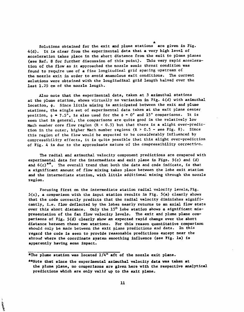
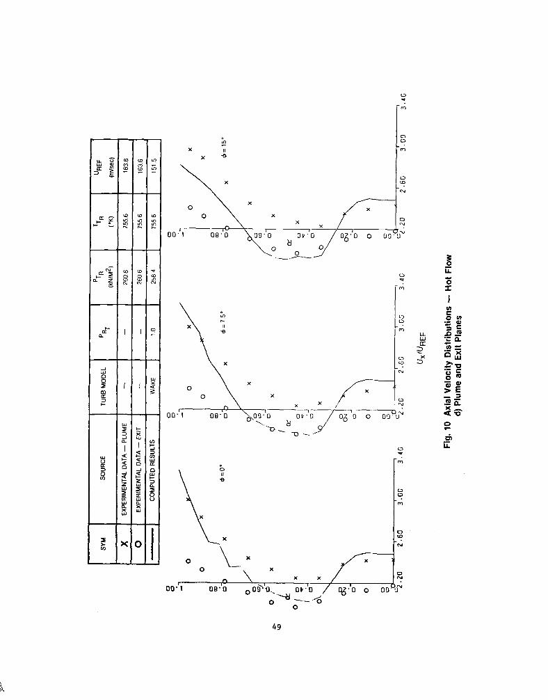
Solutions obtained for the exit and plume stations* are given in Fig. 4(d). It is clear from the experimental data that a very high level of acceleration takes place in the short distance from the exit to plnme planes (see Ref. 8 for further discussion of this point). This very rapid accelera- tion of the flow as it approached the nozzle sonic throat condition was found to require use of a fine longitudinal grid spacing upstream of the nozzle exit in order to avoid anamolous exit conditions. The current solutions were obtained with the longitudinal grid length halved over the last 1.25 cm of the nozzle length.

Also note that the experimental data, taken at 3 azimuthal stations at the plume station, shows virtually no variation in Fig. 4(d) with azimuthal location, #. Since little mixing is anticipated between the exit and plume stations, the single set of experimental data taken at the exit plane center position, + - 7.5", is also used for the $ = 0" and 15" comparisons. It is seen that in general, the comparisons are quite good in the relatively low Mach number core flow region (R < 0.5) but that there is a slight over-predic- tion in the outer, higher Mach number regions (R > 0.5 - see Fig. 8). Since this region of the flow would be expected to be considerably influenced by compressibility effects, it is quite possible that this slight over-prediction of Fig. 4 is due to the approximate nature of the compressibility correction.

The radial and azimuthal velocity component predictions are compared with experimental data for the intermediate and exit plane in Figs. 5(c) and (d) and 6(c)**. The overall trend that both the data and code indicate, is that a significant amount of flow mixing takes place between the lobe exit station and the intermediate station, with little additional mixing through the nozzle region.

Focusing first on the intermediate station radial velocity levels,Fig. 5(c), a comparison with the input station results in Fig. 5(a) clearly shows that the code correctly predicts that the radial velocity diminishes signifi- cantly, i.e. flow deflected by the lobes nearly returns to an axial flow state over this short distance. Only the 15' lobe station shows a significant mis- presentation of the fan flow velocity levels. The exit and plume plane com- parisons of Fig. 5(d) clearly show an expected rapid change over the short distance between these two stations. For this reason quantitative comparison should only be made between the exit plane predictions and data. In this regard the code is seen to provide reasonable predictions except near the shroud where the coordinate system smoothing influence (see Fig. lB) is

apparently having some impact.

*The plume station was located l/4" aft of the nozzle exit plane.

**Note that since the experimental azimuthal velocity data was taken at the plume plane, no comparisons are given here with the respective analytical predictions which are only valid up to the exit plane.

11

The total pressure variations through the nozzle are presented in Figs. 7(c) and 7(d). The intermediate plane comparisons are seen to provide excellent predictions of the high levels of mixing from the initial inlet profiles (Fig. 7(a)) including the details of the azimuthal variations from 4 = 0 to 15O. Solutions at the exit plane are shown in Fig. 7(d). Although the data shown was obtained at the plume station, it is believed representative of exit plane data due to the small level of viscous stresses active in this

region of the flow. These data clearly indicate that the two streams have virtually fully mixed out In both the radial and azimuthal directions and have virtually eliminated the total pressure differences between the fan and engine flow which were evident at the inlet station, (see Fig. 7(a)). The mixer code reasonably well predicts this behavior except for a slight degree of residual total pressure variation for R > 0.5 where compressibility effects may be significant, as evidenced by the local Mach number profiles in Fig. 8. The overall pressure levels are quite accurate showing only a very small under- prediction by the code.

5. Mixer Nozzle Flow - Hot

(a) General Description ------- --

The principal feature of this test case was that it was a virtual re- production of the cold flow test case described above (see Fig. l(a) and (b)), except that the engine core flow was operated at a temperature of 756°K (1360'~) producing a 60% increase In the engine core flow velocity level. The objective of the current study was to directly assess the code's ability to predict the details of the crucial temperature mixing of the cold fan and hot engine flows.

(b) +lut Profiles -----

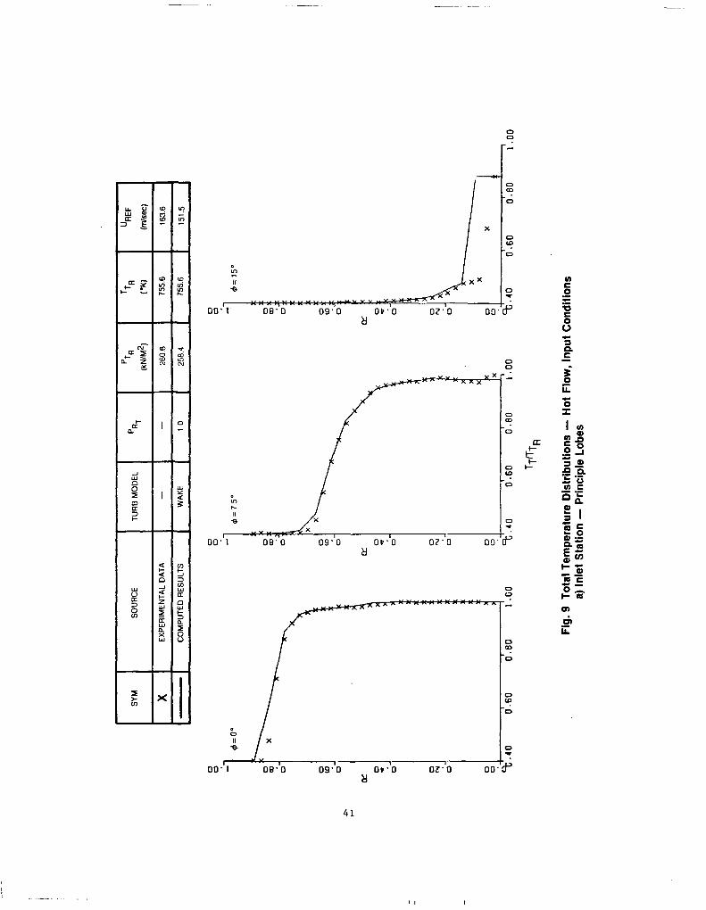
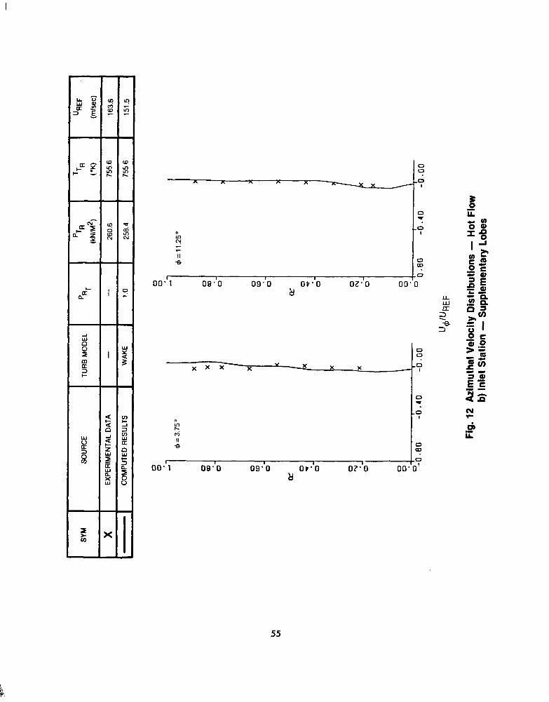
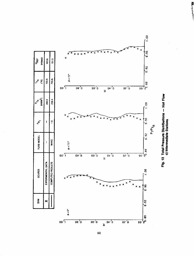
The input conditions and finite difference mesh for this case were virtually identical to those employed for the cold flow caBe (see Fig. l(a)) except that here the experimentally measured total temperature levels at the Inlet station were also interpolated and extrapolated to grid points. The input total tem- perature profiles are shown in Figs. 9(a) and (b), with the velocity distri- butions given III 10(a) and (b), 11(a) and (b), and 12(a) and (b). The analytical curve fit Is Been to provide an excellent representation over the majority of the input plane except for the slight discrepancy in representing the engine flow under the fan lobe (0 = 11.25' and 15O of Figs. 9 through 12) vhere only total temperature and pressure measurements were available. As in the cold flow case, the axial velocity levels were approximated in thie region using the measured total pressures of Figs. 13(a) and (b) with the aosumption of a constant static pressure. The coarseness of the total temperature profiles near R - 0 and 0 - 11.25' and 15O in Fig. 9 is due to the use of a coarse numerical mesh in this region. The total pressure profiles that are pre- dicted by the mixer code at the Inlet station are shown in Fig. 13(a) and (b).

12

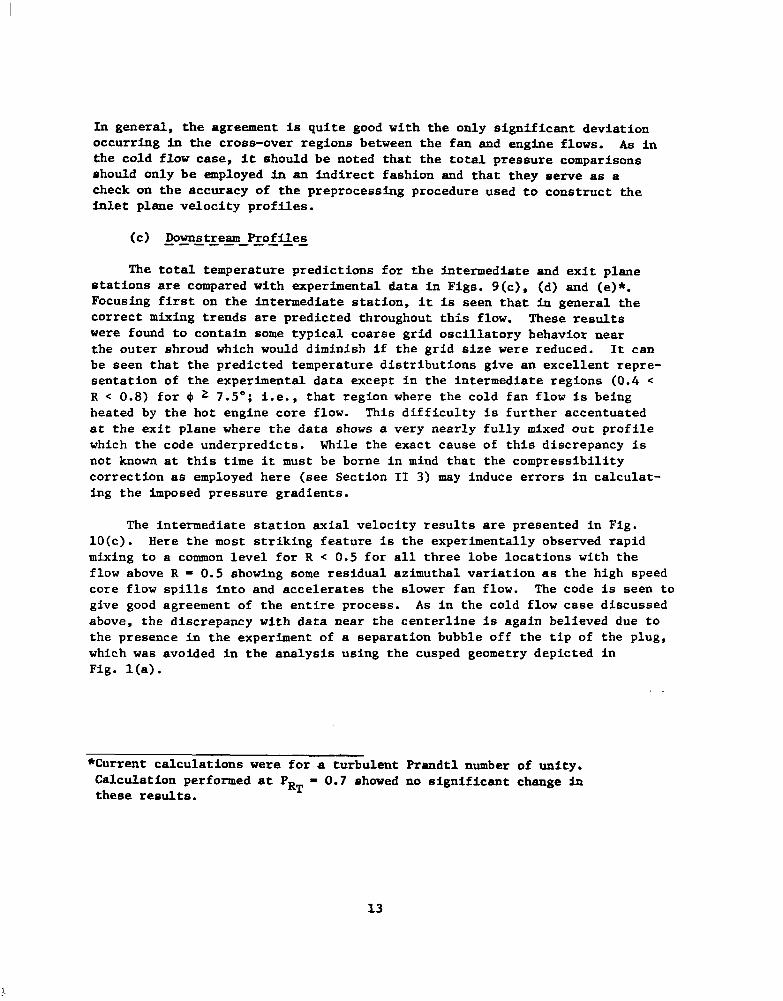
In general, the agreement is quite good with the only significant deviation occurring in the cro6s-over regions between the fan and engine flows. A6 in the cold flow case, it should be noted that the total pressure comparisons ohould only be employed In an indirect fashion and that they eerve as a check on the accuracy of the preprocessing procedure used to con6truct the inlet plane velocity profiles.

(c) Downstream Profiles --a-------

The total temperature predictions for the Intermediate and exit plane stations are compared with experimental data in Figs. S(c), (d) and (e)*. Focusing first on the intermediate station, it is seen that in general the correct mixing trends are predicted throughout this flow. These results were found to contain Borne typical coarse grid oscillatory behavior near the outer shroud which would diminish if the grid size were reduced. It can be seen that the predicted temperature distributions give an excellent repre- sentation of the experimental data except in the intermediate regions (0.4 < R < 0.8) for 4 2 7.5"; i.e., that region where the cold fan flow is being heated by the hot engine core flow. This difficulty is further accentuated at the exit plane where the data shows a very nearly fully mixed out profile which the code underpredicts. While the exact cause of this discrepancy is not known at this time it must be borne in mind that the compressibility correction as employed here (see Section II 3) may induce errors in calculat- ing the Imposed pressure gradients.

The intermediate station axial velocity results are presented in Fig. 10(c). Here the most striking feature is the experimentally observed rapid mixing to a common level for R < 0.5 for all three lobe locations with the flow above R = 0.5 showing 6ome residual azimuthal variation as the high speed core flow spills into and accelerates the slower fan flow. The code is seen to give good agreement of the entire process. As In the cold flow ca6e discussed above, the discrepancy with data near the centerline is again believed due to the presence in the experiment of a separation bubble off the tip of the plug, which was avoided in the analysis using the cusped geometry depicted in Fig. l(a).

*Current calculation6 were for a turbulent Prandtl number of unity. Calculation performed at P

RT - 0.7 showed no significant change in

these resulte.

13

The axial velocity distribution of Fig. 10(d) shows that as the flow proceeds to the plume plane, azimuthal mixing is virtually completed. Note that the exit plane data was only measured at the #I - 7.5O location but It has been displayed at + - 0' and 15O under the assumption that mixing was complete there as well. It is seen that the code provides a qualitatively correct prediction of the drastic changes to the profiles that occur between the intermediate and exit planes, with apparently an underprediction of the degree of mixing that has taken place in this highly accelerated flow.

The intermediate and exit plane radial and azimuthal velocity distributions are shown in Fig. 11(c) and (d) and 12(c). With regard to the intermediate station, it is seen in Figs. 11(c) and 12(c) that the code reasonably well predicts the overall decay of velocity levels from the inlet station values of Fig. 11(a) and 12(a) with only small deviation6 for the radial velocities at the 4 - 0 and 15' locations. Note from Fig. 12(c) there i6 a limited amount of swirl in the center region of the core flow (R c 0.1). As discussed in Vol. I (Ref. 8) this apparently represents a spun up vortex that originates in swirl vanes of the test configuration upstream of the mixer lobes. Fortunately this effect is small and appear6 confined to the center region of the core flow.

Proceeding to the plumeplane,attention Is first focused on the radial velocities of Fig. 11(d). Since the plume plane data shows no azimuthal variation, it is reasonable to assume the exit plane flow is independent of 9 as well. Thus the single exit plane measurement taken at I$ = 7.5 has been repeated at 0 - 0 and 15'. Comparison of the predicted results at the exit plane are very encouraging at the 0 - 0 location. However, at I$ - 7.5 and 15O significant differences are encountered. It is surprising to encounter these large azimuthal variations in the predicted results, when there were no significant variation in the intermediate plane predictions nor in the measured plume plane values taken just aft of the exit plane. Again there exists the possibility that the approximate nature of the com- PTeS6ibilitY correction used In the exit plane region is the casue of the discrepancy.

The$otal pressure predictions from the code are compared with experimental data at the Intermediate and exit planes in Figs. 13(c) and 13(d). In general, the comparisons at the intermediate station are excellent except for a slight difference near the shroud at I$ - 7.5'. This seems tracable to the inlet total pressure profiles shown in Fig. 13(a) where a slight over-prediction was encountered for I$ - 0 0 . The remainder of the profile is very well repre- sented by the predicted results ,xcept naar the core where perhaps some of the residual swirl observed in Fig. 12(c) is causing a drop in the experi- mentally measured total pressure levels.

14

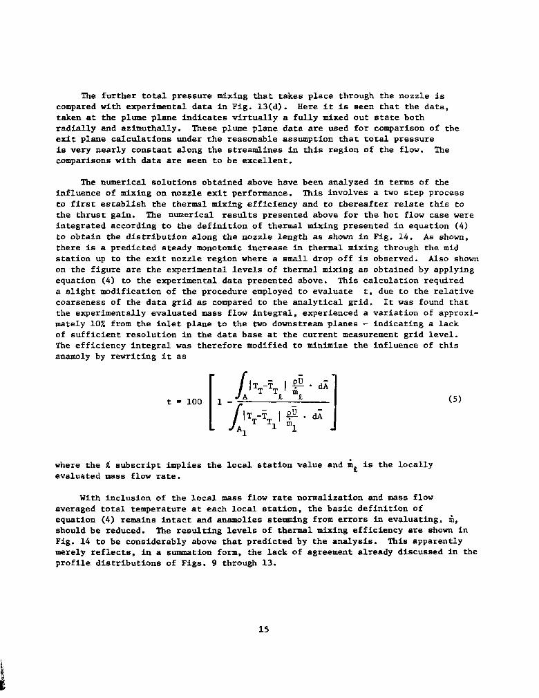
The further total pressure mixing that takes place through the nozzle is compared with experimental data In Fig. 13(d). Here it Is seen that the data, taken at the plume plane Indicates virtually a fully mixed out state both radially and azimuthally. These plume plane data are used for comparison of the exit plane calculations under the reasonable assumption that total pressure is very nearly constant along the streamlines in this region of the flow. The comparisons with data are seen to be excellent.

The numerical solutions obtained above have been analyzed in terms of the influence of mixing on nozzle exit performance. This involves a two step process to first establish the thermal mixing efficiency and to thereafter relate this to the thrust gain. The numerical results presented above for the hot flow case were integrated according to the definition of thermal mixing presented in equation (4) to obtain the distribution along the nozzle length as shown in Fig. 14. As shown, there is a predicted steady monotomic increase in thermal mixing through the mid station up to the exit nozzle region where a small drop off is observed. Also shown on the figure are the experimental levels of thermal mixing as obtained by applying equation (4) to the experimental data presented above. This calculation required a slight modification of the procedure employed to evaluate t, due to the relative coarseness of the data grid as compared to the analytical grid. It was found that the experimentally evaluated mass flow integral, experienced a variation of approxi- mately 10% from the inlet plane to the two downstream planes - indicating a lack of sufficient resolution in the data base at the current measurement grid level. The efficiency integral was therefore modified to minimize the influence of this anamoly by rewriting it as

(5)

where the li subscript implies the local station value and in. is the locally evaluated ma86 flow rate.

With Inclusion of the local ma66 flow rate normalization and mass flow averaged total temperature at each local station, the basic definition of equation (4) remains Intact and anamolles stemming from error6 in evaluating, 6, should be reduced. The resulting level6 of thermal mixing efficiency are shown in Fig. 14 to be considerably above that predicted by the analysis. This apparently merely reflects, In a summation form, the lack of agreement already discussed In the profile distributions of Figs. 9 through 13.

15

Further verification of the experimental result6 presented In Fig. 14 is available from independent thrust measurement tests taken on similar mixer nozzle configuration6 by FluiDyne Corporation for Pratt & Whitney Aircraft Company (see Ref. 9). Work done at P&WA (Ref. 10) indicated that the thermal mixing t, and force mixing, f, should be similar (to within f 3%) thus the data of Ref. 9 can be employed directly here. Figure 15 present6 a comparison of the current experimental and numerical results to experimentally measured levels (Ref. 9) taken at higher value6 of the ideally mixed Mach number at the mixing plane*. The current results appear to be consistent with a reason- able extrapolation of the previous force te6t data while the numerical results yield much lower mixing levels.

IV. CONCLUSIONS

A critical assessment ha6 been conducted of a computational technique for predicting the forced mixing of a hot core and cold fan flow. It was found that in general the code provided reasonably accurate prediction of the pressure and therm61 mixing of the two streams in the low speed portions of the duct region. These results were found to be highly sensitive to the inlet flow conditions - indicating a need for experimental data resolution somewhat finer than that anticipated here. It was also found that the thermal mixing was underpredicted in the highly accelerated nozzle exit region.

* The ideally mixed Mach number is obtained through solution of the conservation equations for constant area mixing of the fan and core flow to a uniform state.

16

1.

2.

3.

4.

5.

6.

7.

8.

9.

V. REFERENCES

Anderson, B. H., and L. A. Povinelli: *'Factors Which Influence the Behavior of Turbofan Forced Mixer Nozzle", AIAA Paper presented at the AIAA 19th Aerospace Sciences Meeting, St. Louis, Missouri, Jan. 12-15, 1981 and NASA Technical Memorandum 81668.

Anderson. 0. L.: "Calculation of Internal V~BCOUS F~OWB in Axisymnetric Duct6 at Moderate to High Reynolds Numbers". Int. J. of Computer6 and Fluids, Vol. 8, No. 4, Dec. 1980, p. 391-411.

Rreskovsky, J. P., W. R. Briley, and H. McDonald: "Turbofan Forced Mixer-Nozzle Internal Flowfleld - Vol. 3, A Computer Code for 3-D Mixing in Axisymmetric Nozzles", NASA CR-xXxX, April 1981.

Heck, P. H.: "Jet Plume Characteristics of 72-Tube pnd 72-Hole Primary Suppressor Nozzles", General Electric Co. Flight Propulsion Division Technical Memorandum No. T. M. 69-457, July 1969.

Coles, D. E. and E. A. Hirst: "Proceedings-Computation of Turbulent Boundary Layers 1968." AFOSR-IFP-Standford Conference, August 1968.

Barber, T. J., P. Raghuraman, and 0. L. Anderson: "Evaluation of an Analysis for Axisymmetrlc Internal Flows in Turbomachinery Ducts", appearing Flow in Primary Non-Rotating Passages in Turbomachines, published by the American Society of Mechanical Engineers, New York, 1979.

Roberts, Glyn 0.: "Computational Meshes for Boundary Layer Problems". Proceedings of the Second International Conference on Numerical Methods in Fluid Dynamics. Volume 8 of Lecture Notes in Physics, Maurice Holt, ed., Springer-Verlag, 1971, pp. 171-177.

Paterson, R. W.: "Turbofan Forced Mixer-Nozzle Internal Flowfield, Vol. 1 - A Benchmark Experimental Study", NASA CR-XXXX, April 1981.

Morgan, K. K. and J. H. Berger: "Hot/Cold Flow Model Tests to Determine Static Performance of 1/7th Scale JT8D-209 Mixer Exhaust Nozzles" FluiDyne Report 1119, FluiDyne Engineering Corp. Mlnn. Minnesota, Nov. 1977.

10. Rardas, G. E., private communication, Pratt and Whitney Aircraft Company, East Hartford, CT 1980.

17

w

-

-

18

19

i tk i ‘\

2.8

2.4

2.0

1.6

0.8

i 01

1

I - I

SYM 1 X/D [ REMARKS 1 1 l 1 2.79 1 EXPDATA.REF4 1

-- -- 2.79 PRESENT RESULTS

0 5.50 EXP DATA, REF 4

1 5.50 PRESENT RESULTS

0.2 0.4 0.6 0.8

“‘“FIEF

Figure 2. Hot Jet Test Case a) Axial Velocity Profile Comparisons

20

I

?.8 -

!.O -

.6 -

I.8 -

SYM WD REMARKS

0 2.79 EXP DATA, REF 4

-m-w 2.79 PRESENT RESULTS

0 5.50 f%XP DATA, REF 4

5.50 PRESENT RESULTS

0

0 0

\ \

0

0.6 0.8 1

T/T TR

Figure 2. Hot Jet last Case b) Total Temperature Profile Comparisons

21

Figure 3. Fraser Flow Test Case a) Centerline Velocity Comparisons

22

SYM

0

E -w-B

---

REMARK

EXP DATA, FIEF 5

WAKE MODEL, by CONSTANT

TKE MODEL, by CONSTANT

WAKE MODEL. AY VARIABLE

Figure 3. Fmser Flow Test Case b) Centerline Pressure Comparhns

23

- ‘I

SYM I REMARK 1

0 1 EXPDATA. REF 5 I

- WAKE MODEL, by CONSTANT

- - -- TKE MODEL. Ay CONSTANT

- - - WAKE MODEL. Av VARIABLE

0.004 -

0.003 -

0.002 -

0.001 -

OO 0.1 0.2 0.3

X/D

Figure 3. Fraser Flow Test Cese c) Skin Friction Comparisons

24

. i

I 1 1 00’ I I 09’0 I 09’0 OV’O 02’0 00 &I

b ::

i X

0 m . ‘0

0 v . 0

iii P

‘0

0

0” P

0

0 *

0

25

I- B

J--J- o 2 &

i r I I I I

00’ 1 OR’0 09’0 00-o 02’0 00 &I

0 Q) ‘0

0 0 0

z P

. c L-5 4

, 1 I I I s 00’ I 09’0 09’0 OV’O 02’0 0o.f

tl

26

I

r I 00’ I 1 OR’0 1 I

09’0 OP.0 02’0 00 tl

2 ‘0

0 t

‘0

Ei

P

J , , ‘ , oo[ 00’ 1 08’0 09’0 ot-0 02’0

. 0

:

b I 00‘ I

I 00’0 09’0

, I DC’0 02’0 00

Ii

27

X X

X

3 X X

0 X X’ 0

x

0 . 2

A X

0 4 0 0 0 0 0

\ 1 I I I, I 00’ I OR’0 09’0 0)‘0 02’0 OC

&I

X X

X

28

X X

X

8 -0 1

0 t -0

29

.

X X-

I I I I 1

00’ I 08’0 09’0 or-0 02’0 01 tl

E 0 I

0 w

, .O

I

0 aD

.O

D’

30

X X X x x

1 I I I I 00’ I DA’0 09’0 OP.0 02’0 00

tl

z

.O I

0 *

. .O

I

0 (P

.O

I’

0 0

0 I

0 w

0 I

0 al

.O

3’

0 w

-0 I

D 0 :: 0

rT)

1 1 1 I 1 00’ I oe.0 09'0 ot-0 02'0 oo.o?

&I

31

c n!! ,: ; ~~

O0 In rc’

:: I I

00’ 1 I

OR’0 I

09’0 Oh’0 I

02’0 00 ti

x X X X X

0 *

. -0

I

00

t 1 I

00’ I 1

OB’O I I

09’0 or-0 02’0 00-o’: &I

32

-

0 rr! r-

5

I 1 I 1 I 00’ 1 08’0 03’0 0)‘0 02’0 00

tl

t 'C

'C

X X

X X X

. 0 &

t I I , , 00'1 OR'0 09'0 or.0 07-o 00' o7

c- 8

33

=z - . -

= “r i’ t

E

c o!=

Y 5 s:

* X X y x d

4

I , r 1 r 00'1 08'0 09'0 or-0 02'0 00

tl

- x x -

X X Y x x

f3 . .O

I

0 *

. ,O

,

0 m

-0

II’

-0 I

0 *

,O I

0

r ci

4 tz

I r I I 1 3

00'1 08'0 09'0 tl o"'o'

02'0 00' 0':

34

8 . -0 x X X x * I

X 1c

. 0

::

35

I I 00’ I

I I I 08’0 09’0 OP.0 02’0 00’

tl ,d

is

s

0

s

0

b

::

Ei I

00' I I I I 1 00'0 09'0 Dt'0 02'0 0o.f

&I

36

a< ct t

I- I?

z

xX

iti .

0

z .

. 0

tt ,:

4 aD (D

I . I 00’1 1 I 1

09’0 09’0 Ot’0 02’0 00-f 8

37

b r;

: z

r 1 1 r 1 I 00’ I 08’0 09’0 or.0 02'0 0o.L-P

8

%

0

z.z

0

. 0 II

8 Et I I 1 1 1

00'1 00'0 09'0 OC'O 02'0 00.6; 8

38

1 I I I I 00' I 00'0 09'0 ot-0 02'0 00

tl

8

X x x x 1: z?l 0

b r-:

k

I I I I I 00' I OR'0 09'0 ot'0 02'0 00

21

x x x x

x x x x xxxxxx

b :

* I 1 I I 00’ 1 00’0 09’0 DC’0 02'0 01

tl

39

40

00

41

I-

n?

:: XX

Y., I

00’ I 08’0 09’0 OC’O 07’0 00 tl

0 u)

‘0

0

;

42

I I 00' I OR'0 09'0 OP.0 07’0 05

ii

b II 8

I 1 00’ 1 OR’ 0 09’ ------& 0 Ok’ 0 07’0 -

8

43

00

0 L . R 0

,’ : 0 w

‘II I 1 08’0 Ob’o ..I. 09’0 07’0 0O.F

I I 1-v 00’ I 08’0 09’0 OC’O 07’0 00

tl

a t!- 2-

44

I

/ x x i X

X 4 I I I I I

00’ 1 OR’0 09’ 0 OP‘O 07’0 OI

tl

r; X 4 I I 3 I I 00’ 1 08’0 09'0 OC' 0 07' 0 00

tl

/- -

45

1 I I I I 00’ I 08’0 09’0 Ob’d oz.0 00-e

tl

22 0

0 w

0

0” .

I I I I 1 1- 00’ I 08’0 09~0 Ob’O oz.0 oo*f

tl

46

I I I 00’ 1 08’0 09’0

!V-& Ob’ 0 07’0 . .

tl

I I I 00’ I 08’0 09’0

tl

47

ap l- - -

0 al

0

0 w

0

0 In

4 iii

I I I 1 I 00’ 1 OR’0 09’0 Ob’ 0 07’9 O!J’ 11”

a

I . 1 1 I I 1 I

00’ 1 OR’0 09’0 OP.0 07’0 0O.F ti

48

X X

x X

x

00‘ I 08’0

y IF

09’0 OP.0

O &o O Oi3’0 O OL; \ --..---

I I I I 1 I

08’0 09’0 OP.0 07’0 00’ oy tl

I 00’ I

I 7 08’0 09i----- OP.0 07’0 00’0

tl

0 0

:

I I I I I 00’ I 08’0 09’0 Ob’O 02’0 00

8

50

I I 1 1 I

00’ 1 08’0 09’ 0 OP.0 07’0 00 tl

0 I

0 (D

,?

0 w

I I I , I 1

00’ I 08’0 09’0 Ob‘O 02’0 00’ % tl

51

z

60 I

0 -

-0 I

b

1: iii

I I 1-1 0

00’ I OB’O 09’0 OP.0 07’0 00’ 3

tr

52

I- n=

53

A

R

I I I 00’ 1

I I 08’0 09’0 OP.0 07’0 00

tl

X a y x

I I I I I I

00’ I 08’0 09’0 OP.0 07’0 00’ cl7 tl

0” X Y X

A A .- -0 X I

0 0

4

I I I I I 00’ 1 08’0 09’0 Ob’O 02’0 00

tl

IO w

-0 t

0 aD

. .O

3’

54

G

II 8

I I I I 00’ I

I 08’0 09’0 OP.0 02’0 00

tl

z

x x x -x X x -0 I

. .- . ..-. -

Y *

X

0 v, r-

: I I 1

00' I 08'0 09'0 ------TO 07?0 03 tl

x Y X X Y a a

X

k3 LO

I

I I I I 1 I 00’ 1 08’0 09’0 or.0 07’0 oo.loo

tl

56

-VA x X X

b

i

1 I I 1 I 00’ 1 OB’O 09’0 OC’O 07’0 09

b

OO”1 08”O 09.‘0 OP.‘0 oz.‘0 Oil b

is

X Y 1-0 x x X

X I X X

-0 I

I I I I I 00’ 1 08’0 09’0 OP.0 07’0

u

57

1 I 00’ I

I I 00’0

I 09’0 OP.0 02’0 00

tl

b

4

I 00’ I

I I I I 00’0 09’0 0,.0 07’0 0t

&I

58

c

CF

r I 00’ I

I I 00’0 09’0

I Ok’ 0 07’0 00

8

1 I I 00’ 1

I 08’0 09’0

I OP.0 OZ’O 00

tl

59

-x - X

X- xxxx xxxxxxxxxx it!

X

-‘I-

0

:

0

Fn II

8 z

I I I 00’ I

I OR’0 09’0 OP.0 07’0 0o.f

a

X

xx H”x x .rm

xxx x 0,

60

I- L=

08.10 09 .‘o I I

olr 0 07’0 00 &I

x x x x - X

x y” x x

I I I I 00’ 1 OR’ 0 09’0 Or’ Ll 07’0 03

b

I:

I’ I

CE ‘0

P % I-

N n m

‘0

,----- I I I I 00’ I 08’0 09.0 OP’O 02’0 00

&I

61

1oc

8C

20

a

INITIAL PLANE

INTERMEDIATE PLANE

l

EXIT PLANI

l EXPERIMENTAL RESULT - NUMERICAL RESULT

Fig. 14. Nozzle Thermal Mixing Distribution

62

P CURRENT NUMERICAL SOLUTION

T CURRENT EXP DATA (REF. 8) A

Ezl EXP THRUST DATA (APP B)

EXTRAPOLATION (APP B)

v CURRENT MIXER MODEL

I /I I I 0 0.1 0.2 0.3 0.4 C

IDEALLY MIXED MACH NUMBER AT MIXING PLANE

Figure 15 - Exit Mixing Level Based on Thrust

63

APPENDIX A

USER'S MANDAL - MIXER NOZZLE CODE

1. Pre-Analysis Element

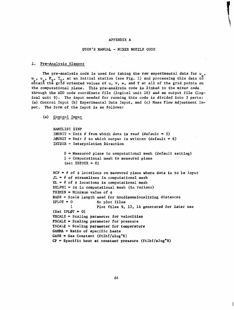
The pre-analysis code is used for taking the raw experimental data for u ,

;&,;f 'T' TT' at an initial station (see Fig. 1) and processing this data tg

the gr d oriented values of u, v, w, and T at all of the grid points on the computational plane. This pre-analysis code is linked to the mixer code through the ADD code coordinate file (logical unit 16) and an output file (log- ical unit 9). The input needed for running this code is divided into 3 parts: (a) Control Input (b) Experimental Data Input, and (c) Mass Flow Adjustment In- put. The form of the input is as follows:

NAMELIST $INP INDNIT = Unit # from which data is read (default = 5) J@JNIT = Unit I to which output is written (default = 6) INTDIR = Interpolation Direction

0 -+ Measured plane to computational mesh (default setting) 1 -t Computational mesh to measured plane (set INTDIR = 0)

NCP = # of @ locations on measured plane where data is to be input JL = d of streamlines in computational mesh KL= # of Q locations in computational mesh DELPHI = A$ in computational mesh (in radians) PHIMIN = Minimum value of $I RADR= Scale length used for nondimensionalizing distances IPLOT = 0 No plot files

(Set IPLiT = 0) Plot files 9, 12, 14 generated for later use

VSCALE = Scaling parameter for velocities PSCALE = Scaling parameter for pressure TSCALE- Scaling parameter for temperature GAMMA = Ratio of specific heats GASR = Gas Constant (ftlbf/slugOR) CP = Specific heat at constant pressure (ftlbf/slugOR)

64

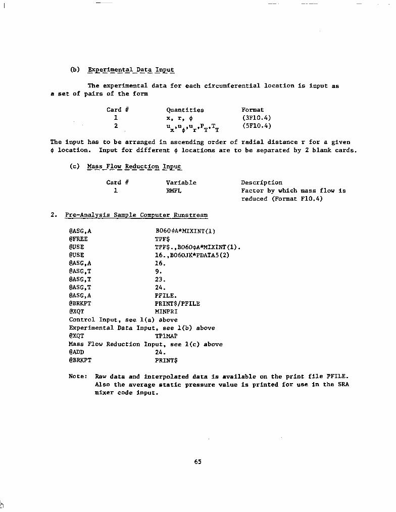
(b) ExEez@ental Data InEuL ------

The experimental data for each circumferential location is input as a set of pairs of the form

Card # Quantities Format 1 x, r, 4 (3F10.4) 2 ux9u ,u $J J' ,T r T T

(5F10.4)

The Input has to be arranged in ascending order of radial distance r for a given $ location. Input for different $I locations are to be separated by 2 blank cards.

(c) ga=s-F&n#&efiuLtLo; LnEuL

Card d Variable Description 1 RMFL Factor by which mass flow is

reduced (Format F10.4)

2. Pre-Analysis Sample Computer Runstream

@ASG,A BO604A*MIXINT(l) @FREE TPF$ @USE TPF$.,BO6O$A*MIXINT(l). @USE l6.,B060JK*PDATA5(2) @ASG,A 16. @ASG,T 9. @ASG,T 23. @ASG,T 24. @ASG,A PFILE. @BRKPT PRINT$/PFILE @XQT MINPRI Control Input, see l(a) above Experimental Data Input, see l(b) above @XQT TPlMAP Mass Flow Reduction Input, see l(c) above @ADD 24. @BRKPT PRINTS

Note: Raw data and interpolated data is available on the print file PFILE. Also the average static pressure value is printed for use in the SRA mixer code input.

65

Note: Unit 9 contains the information on u, v, w and T needed in the SRA mixer code and should be added after namelist SIN7 (Ref. 3) for running the mixer code.

3. Post Processor Element

After the mixer code has been run, it is necessary to move the computed results back to the measuring planes and resolve the velocities into cylindrical Cartesian coordinates to facilitate comparison with experimental data. This process is essentially the reverse of the preanalysis process. This post pro- cessor is linked to the mixer code through the ADD code coordinate file (log- ical unit 16) and an output file (logical unit 8) that contains the computed flow field from the mixer code. The form of input is as follows:

Namelist $SRAINP

JL= No. of radial grid points KL= No. of circumferential grid points NSRA = No. of axial stations used in mixer analysis NADD = No. of axial stations in the ADD code coordinate file NPIANE = No. of data planes at which this analysis is performed XPLANE= NPLANE values of axial distance where this analysis is performed (ft) XENTER = Location of inlet data plane (ft) USC = PSC =

Reference Velocity (ft/secJ Reference pressure (lbf/ft >

TSC = Reference temperature (“R) ISUNIT = logical unit # for flow field file (default to 8)

4. Post-Analysis Sample Computer Runstream

@ASG,A BO~@$JA*MIXINT(~) @FREE TPF$. @USE TFP$., B060$A*MIXINT(l). @USE 16., B060JK*PDATA5(2) @ASG,A 16. @USE 8., VATSAN*JETDTB. @ASG,A 8 @ASG,T 20. @ASG,A PFILE. @BRKPT PRINT$/PFILE @XQT XFSRA Input Namelist $ SRAINP discribed above @BRKPT PRINTS

66

Note: The printfile PFILE contains the velocities, pressure and temperature in self-explanatory form for NPLANE nuuber of x stations.

67

APPENDIX B

Pratt & Whitney Aircraft Mixer Nozzle Flow Analysis

G. F. Rardas W. M. Presz, Jr.

Pratt & Whitney Aircraft/Commercial Products Division

INTRODUCTION

Pratt & Whitney Aircraft/Commercial Products Division was involved in technical support effort under a (P&WA/CPD) subcontract to United Technologies Research Center (LITRC) for the Aircraft Engine Turbofan Forced Mixer Analysis and Experiments Program (NASA Contract NAS3-20951). Principal aims of the contract included (1) the development of an advanced computer code for the analysis of the mixing process occurring between the core and fan flows in a turbofan mixed-flow exhaust system, and (2) the conduct of flowfield measure- ment experiments to obtain data for verification of the developed computer analysis and for the establishment of a unique mixer flowfield data base. In support of this contract, P&WA/CPD completed the following work: (a) provided mixer test hardware; (b) consulted on test formulation and procedures; (c) predicted mixer duct velocity profiles and compared results to data; (d) predicted mixer lobe losses and compared results to data; (e) predicted mixer nozzle performance using previous experimental results; and (f) consulted on the evaluation of the developed computer analysis. This appendix summarizes the work conducted by P&WA/CPD.

Discussion

Test Hardware

Pratt 8 Whitney conducted hot and cold flow model tests of thirty-eight candidate 12 lobe forced mixer configurations for the JT8D engine in 1977. One of these configurations, with a scarf angle of -12', was selected as the test configuration for this program. It is shown schematically in Figure B-l. This forced mixer was selected for two reasons: (1) it represented a realistic mixer for a current engine, and (2) existing thrust and nozzle exit plane profile data was available. This configuration was provided to UTRC for use in the experimental portion of the contract effort. The test hardware assembly is shown schematically in Figure B-2.

68

During initial tests using the selected mixer, it was determined that UTRC's hot flow test stand was not capable of sustaining the JTBD nozzle pressure ratio at previously tested mass flow levels with the existing exhaust nozzle. The nozzle exit area was decreased to allow simulation of realistic pressure ratios. This modification, introduced sufficient changes in test flow conditions such that the existing thrust and nozzle exit profile information was not directly applicable.

Test Formulation and Procedures

Since the selected forced mixer configuration represented a realistic mixer for a current engine, it was desirable to have a set of test flow conditions which were representative of engine operating conditions at a critical operating point, and which also were similar to previously tested flow conditions. Cruise operation was chosen for simulation and this led to recommending the following reference flow conditions:

1) Charging station engine pressure ratio, PTR/Pamb, of 2.595;

2) Charging station fan to engine pressure split, PTF/PTR, of 0.95;

3) Cold flow test temperature split, TTF/TTR, of 1.00; and

4) Hot flow test temperature split, TTF/TTE, of 0.475.

Actual tested flow conditions for the forced mixer experimental investigation duplicated items 1, 2, and 3. Due to test stand capability limitations, item 4, the hot flow test temperature split, was set at 0.400.

Initial experimental measurements of nozzle exit plane flow velocities using laser velocimetry in a cold flow test indicated that measured velocities were about 5% below ideal axisymmetric inviscid nozzle flow theory values calculated by P&WA. The velocities are obtained by seeding the flow with small particles, reflecting laser light off the particles, measuring the intensity of the reflected light, and converting the measured signal strength to a velocity. A basic assumption is that the particle velocities are representative of the flow velocity, and this is true only if the particle size is small enough for the inertial forces to be negligible. The accuracy of the ideal axisymmetric inviscid nozzle flow theory is well within a 5% error level. This indicated that the seed particles were not being accelerated to true flow velocities at the nozzle exit. Consequently, significant improvements were made by UTRC to the state-of-the-art techniques utilized to generate the seed particles for laser velocimeter measure- ments. The improved techniques were then used through the remainder of the test program.

69

Further assistance was provided to UTRC during the experimental investigations in several ways. First, a normalized velocity parameter was defined for possible use in velocity dat,a presentation. This velocity parameter was based on the local value of the ideally mixed flow velocity for a given axial position in the mixer duct. Comparison of velocity measurements to the local value of the Ideally mixed flow velocity could provide an indication of the local "mixedness" of the flow. Second, a brief analytical study was conducted to investigate the possible effects of mixer duct wall boundary layer behavior on measured variations in nozzle exit velocities with nozzle total pressure changes. The effect was found to be negligible.

Mixer Duct Velocity Profiles

Analytical predictions of the velocity profiles generated through the model mixer duct and near the nozzle exit plane were made for both the cold flow and hot flow tests. Nominal values of the primary and fan flow properties were processed through the P&WA/CPD one-dimensional mixing calculation to obtain ideally mixed flow properties. Calculation of the mixed flow properties assumes the existence of a static pressure balance between the fan and pri- mary flows at the end of the forced mixer lobes. Flowfield calculations were then made for the mixed flow using the transonic internal flow Nozzle Analysis Program (reference B-l). Thus, the predicted flow profiles were representa- tive of the mean properties for a completely mixed flow.

Laser velocimeter data were acquired at three axial locations in the mixer duct using the assembly shown schematically in Figure B-2. Data were taken immediately downstream of the mixer lobes (Station l), at an intermediate location in the mixer (Station 2), and at a location nominally 0.75 cm down- stream of the nozzle exit plane (Station 3). The azimuthal positions at which data were acquired are shown in Figure B-3.

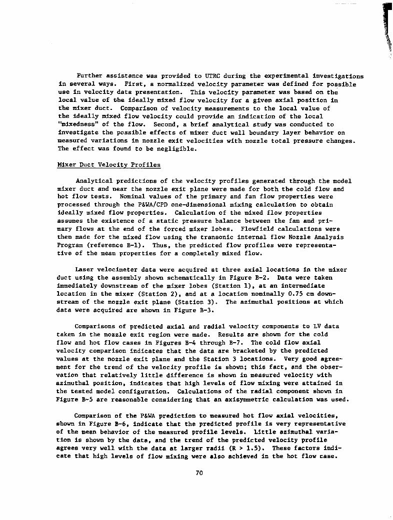
Comparisons of predicted axial and radial velocity components to LV data taken in the nozzle exit region were made. Results are shown for the cold flow and hot flow cases in Figures B-4 through B-7. The cold flow axial velocity comparison indicates that the data are bracketed by the predicted values at the nozzle exit plane and the Station 3 locations. Very good agree- ment for the trend of the velocity profile is shown; this fact, and the obser- vation that relatively little difference is shown in measured velocity with azimuthal position, indicates that high levels of flow mixing were attained in the tested model configuration. Calculations of the radial component shown in Figure B-5 are reasonable considering that an axisymmetrlc calculation was used.

Comparison of the PSWA prediction to measured hot flow axial velocities, shown In Figure B-6, Indicate that the predicted profile is very representative of the mean behavior of the measured profile levels. Little azimuthal varia- tfon is shown by the data, and the trend of the predicted velocity profile agrees very well with the data at larger radii (R > 1.5). These factors lndi- cate that high levels of flow mixing were also achieved in the hot flow case.

70

The predicted hot flow radial velocity profile at Station 3 (see Figure B-7) shows fairly good agreement with the data in the interior portion of the flow. The prediction Indicates the initiation of a radially outward expansion of the flow in the vicinity of the nozzle lip. Such behavior should be expected, since the 2.5 pressure ratio flow should produce an expanding exhaust plume about the nozzle lip.

Total pressure losses through the mixer lobes (i.e., from the charging station to the mixer duct entrance plane) were evaluated from P&WA empirically derived loss relations. These loss relations include approximations for fric- tional losses and an accounting for losses induced by struts and vanes. The resulting predictions of the lobe total pressure losses were compared to the total pressure losses calculated from an averaging of the measurements taken in the UTRC forced mixer model test.

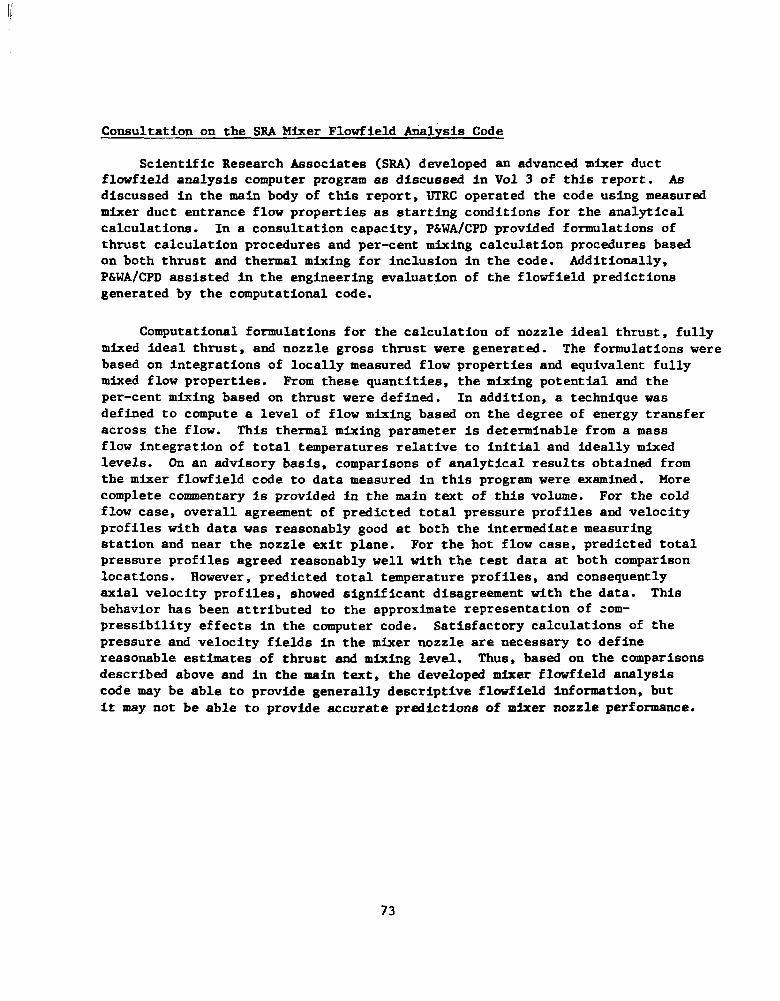
Isobaric contour maps of measured total pressure at the mixer duct en- trance plane were prepared from the cold flow and hot flow data, and these are shown in Figures B-8 and B-9. The isobaric contour patterns are fairly similar and are closely indicative of the mixer lobe shape. The measured total pres- sures and total temperatures were processed through the P&WA Pressure Averaging Deck to obtain stream-thrust averaged total pressure losses. Results are presented as item (a) in Table B-I. The pressure averaging process was performed with both a constant static pressure downstream of the lobes and the local static pressure gradient computed by the transonic internal flow analysis procedure used for the velocity profile predictions. The effect of static pres- sure gradient on calculated average total pressures was found to be inconse- quential to this case.

Total pressure losses through the mixer lobes were computed based on the nominal values of flow properties at the model charging station. The results are shown in item (b) In Table B-I. Very little difference In pressure loss was computed for the cold flow and hot flow cases. This result may be expected since the differences In flow Reynolds number are not significant, and the con- sequent differences in skin friction coefficient are small.

A slight alteration may be noticed in the isobar patterns near the inner wall at the center of the contour maps. This Is possibly a result of varia- tions in the secondary flow patterns established in the forced mixer. An exam- ination of the laser-velocimeter measured radial and azimuthal velocities at the lobe exit plane were used to calculate the incremental equivalent secondaiy flow pressure loss (Item b, Table B-I). This is seen to be approximately 15% of the skin friction loss for the cold flow and hot flow cases. As also shown in Table B-I for the cold flow case, the total estimated pressure loss (item c) is in excellent agreement with the loss calculated from the data (item a). The

* The secondary flow contribution to the total pressure loss Is taken to be the secondary flow dynamic pressure.

71

hot flow case does not exhibit similar closure. However, the difference in the hot flow pressure loss results, as shown by column (c) of Table B-I, appear to be within the measurement accuracy (f 0.5%) of the pressure transducers used in the experiments.

Hixer Nozzle Performance Estimates

Using previously obtained P&WA/CPD data for the type of forced mixer con- sidered in this program, and utilizing a PLWAICPD ideal mixing analysis pro- cedure, estimates of thrust levels that could be produced In the cold flow and hot flow tests of the configuration Investigated in this program were generated.

For the thrust calculation, the flow mixing was assumed to be complete. Review of the UTRC flow measurements indicated this to be approximately correct, i.e., 90%. The P&WA/CPD ideal mixing procedure was applied to core and fan flow properties entering In the mixer duct. Core and fan flow total pressures were calculated using the P&WA/CPD pressure loss relations applied to the nominal total pressures at the charging station. For the cold flow case, this procedure indicated a 0.2% decrease in ideal thrust due to mixing for the completely mixed flow. Including estimated nozzle losses , the cold flow gross thrust calculations would be expected to show a 0.7% decrease through the mixer duct; i.e., the gross thrust based on the nozzle exit properties is 99.3% of the gross thrust based on the duct entrance properties in the cold flow case.

For the hot flow case, the ideal mixing analysis procedure indicated that a 2.6% increase in thrust could be achieved through complete flow mixing. Data from a P&WA/CPD forced mixer model tests conducted in 1977 (reference B-2) were reviewed to establish an estimate for the level of mixing in the research model in this program. For the forced mixer configuration tested, the previous data indicated that 75% mixing, based on thrust, had been achieved. The thrust measurements for the 1977 program were accurate to * 0.25%; this accuracy then represents * 10% in the mixing level for this program. Since the nozzle exit area and hence the mixing plane Mach number was reduced for this program, the 75% mixing level had to be corrected. Other data taken during the P&WA/CPD tests for similar mixers at the same nozzle pressure ratios were used to estab- lish the trend shown in Figure B-10. The slightly longer tailpipe length for the UTRC model could be expected to add a small but relatively negligible ln- crease to the mixing level based on other P&WA/CPD data. As shown in Figure B-10, the UTRC measured mixing level, based on thermal mixing, Is within the projected trend from the P6WA/CPD data. Using the extrapolated value of 97% mixing and including estimated nozzle losses , gross thrust calculations would be expected to show a 2.2% increase through the mixer duct; i.e., the gross thrust based on the duct entrance properties for the hot flow case.

72

Consultation on the SRA Mixer Flowfield Analysis Code

Scientific Research Associates (SRA) developed an advanced mixer duct flowfield analysis computer program as discussed in Vol 3 of this report. As discussed in the main body of this report, UTRC operated the code using measured mixer duct entrance flow properties as starting conditions for the analytical calculations. In a consultation capacity, P&WA/CPD provided formulations of thrust calculation procedures and per-cent mixing calculation procedures based on both thrust and thermal mixing for inclusion in the code. Additionally, P&WA/CPD assisted in the engineering evaluation of the flowfield predictions generated by the computational code.

Computational formulations for the calculation of nozzle ideal thrust, fully mixed ideal thrust, and nozzle gross thrust were generated. The formulations were based on integrations of locally measured flow properties and equivalent fully mixed flow properties. Prom these quantities, the mixing potential and the per-cent mixing based on thrust were defined. In addition, a technique was defined to compute a level of flow mixing based on the degree of energy transfer across the flow. This thermal mixing parameter is determinable from a mass flow integration of total temperatures relative to initial and ideally mixed levels. On an advisory basis, comparisons of analytical results obtained from the mixer flowfield code to data measured in this program were examined. More complete commentary is provided in the main text of this volume. For the cold flow case, overall agreement of predicted total pressure profiles and velocity profiles with data was reasonably good at both the intermediate measuring station and near the nozzle exit plane. For the hot flow case, predicted total pressure profiles agreed reasonably well with the test data at both comparison locations. However, predicted total temperature profiles, and consequently axial velocity profiles, showed significant disagreement with the data. This behavior has been attributed to the approximate representation of corn- pressibillty effects in the computer code. Satisfactory calculations of the pressure and velocity fields in the mixer nozzle are necessary to define reasonable estimates of thrust and mixing level. Thus, based on the comparisons described above and in the main text, the developed mixer flowfield analysis code may be able to provide generally descriptive flowfield information, but it may not be able to provide accurate predictions of mixer nozzle performance.

73

CONCLUSIONS

. Generally favorable agreement was obtained in comparisons of P&WA/cm) velocity profile predictions to laser velocimeter data. This indicates that axisyuunetric internal flow analysis procedures are capable of providing reasonable predictions of mean flow properties in mixer duct flowfields.

. Heasured nozzle exit velocity profiles indicate high levels of flow mixing were achieved in the forced mixer tests. This is in agreement with an extrapolation of available P&WA/CPD forced mixer test data.

. Total pressure losses through the mixer lobe configuration tested at UTRC are dominated by skin friction losses. Secondary flows generated in the mixer lobes are responsible for additional pressure losses, and these losses are relatively constant from cold flow to hot flow.

. The version of the mixer flowfield analysis code developed in this program may be useful in providing descriptive flowfield information for the analysis of mixer nozzles.

74

RECOMMENDATIONS

The Turbofan Forced Mixer Program has revealed several areas where further work is required and recommended. These include the following:

1)

2)

3)

4)

5)

B-l

B-2

Verify the nozzle performance estimates which were based on extrapolations of available data, and verify analytical performance predictions from an improved version of the developed mixer flowfield computer code. Mixer model performance tests should be conducted using the nozzle hardware from this program.

Use the improved laser-velocimeter measurement techniques to expand the generated flowfield measureddata base. Measurements in other mixer nozzle geometries should be taken to provide information for further verification and improvement of 3-D internal flowfield analysis techniques.

Use the improved laser-velocimeter measurement techniques to investigate secondary flow phenomena in mixer duct flowfields. As a first step, a two-dimensional lobe "cascade" facility could be utilized. Such studies could provide a more thorough understanding of the role of secondary flow formation in flow miring.

Develop advanced three-dimensional internal flowfield analysis procedures to predict mixer lobe losses and secondary flow patterns at the lobe exit. This analysis could be linked to the mixer flowfield computer code to provide a complete predictive technique for forced mixers.

Conduct an analytical mixer design study with the lobe and mixer analyses. Test selected concepts to verify and improve the capabilities of the advanced prediction procedures.

REFERENCES

Michael C. Cline, "NAP: A computer Program for the Computation of Two-Dimensional, Time-Dependent, Inviscld Nozzle Flow', LOS Ahmos Scientific Laboratory Report LA-5984, January 1977.

J. K. Morgan and J. II. Berger, "Hot/Cold Flow Model Tests to Determine Static Performance of l/7 - Scale JT8D-209 Fixer Exhaust Nozzles", FlulDyne Report 1119, FluiDyne Engineering Corp., Minneapolis, EN, November, 1977.

75

TABLE B-I

STREAM-THRUST AVERAGED TOTAL PRESSURE LOSSES THROUGH MIXER LOBES

Item Cold Flow Hot Flow

a) % Apt/P, from data 0.5409 0.6279

b) X AP,/Pt from loss relations % APt/Pt, equivalent secondary

flow pressure loss

0.4660 0.4180

0.0655 0.0605

c) Estimated total X Apt/P, 0.5315 0.4785

d) Loss difference = data-estimate 0.0094 0.1494

76

A

1

I I I . I I

TAILPIPE WALL

a) SECTION B-B

0.44 cm

0.62 cm RADIUS

b) SECTION A-A

Figure 6.1 - Mixer Lobe Geometry Definition

77

78

# = 11.3 deg INTERSECT10 r = 4.069 cm NOZZLE WALL

6 = 15 deg INTERSECTION

----

----#=OO

# = 3.75 deg INTERSECTION r = 7.666 cm

HUB #= 0 deg INTERSECTION r = 7.930 cm

Figure B-3 - Mixer Lobe Geometry

79

COMPARISO* OF ?REDtCTloN TO LV DATA

a--

- PREDICTION 0 DATA.610’

0 DATA, 6’17.5’

0 DATA, 8- 15’

24+0 1.0 2.0 LD 6.0

RADIUS, cm

FIGURE 8.4 - COLD FLOW AXIAL VELOCITIES NOZZLE EXIT REGION

80

COMPARISON OF PREDICTION TO LV DATA

STATION 3 AX - 0.75 cm

I

- PREDICTIDN

is

DATA, 8 - 0’ DATA, 8 - 7.6’

0 DATA,6- lb

EXIT PLANE

I I I I 1 1.0 2.0 3.0 4A 6.0

RADIUS, cm

FIGURE B-5 - COLD FLOW RADIAL VELOCITIES NOZZLE EXIT REGION

81

COMPARISON OF PREDICTION TO LV DATA

PREDICTION

0 DATA, l9 - 00

DATA, 8 = 7.B

DATA.6 15”

49

I 3601 I I I I I 0 1A 2.0 3.0 4.0 61

RADIUS, cm

FIGURE B-6 - HOT FLOW AXIAL VELOCITIES STATION 3

82

lCOMPARlSON OF PREDICTION TO LV DATA

- PREDICTION

0 DATA,hP

0 DATA, 8 - 7.5O

0 DATA.6150

RADIUS, cm

FIGURE B-7 - HOT FLOW RADIAL VELOCITIES STATION 3

83

COLD FLOW TEST - STATION 1 MIXER DUCT ENTRANCE

NO. WPAMB m- 1 2.565 2 2.552 3 2.638 4 2.524 5 2511 6 2.497 7 2.484 8 2.470

FIGURE B-8 - TOTAL PRESSURE ISOBARIC CONTOUR MAP

84

HOT FLOW TEST - STATION 1 MIXER DUCT ENTRANCE

NO. PTiPAM8 - 1 2.865 2 2.652 3 2.638 4 2.624 5 2.611 8 2.497 7 2.484 8 2.470

FIGURE B-9 - TOTAL PRESSURE ISOBARIC CONTOUR MAP

85

100

8C

7c

60

I f

CURRENT EXP DATA (REF. 8)

ml EXP THRUST DATA (APP B)

EXTRAPOLATION (APP B)

/

CURRENT MIXER MODEL

0.1 0.2 0.3 u.4

IDEALLY MIXED MACH NUMBER AT MIXING PLANE

Figure B.10 - Mixing Performance Trend

86

1. Report No. 2. Government Accession No. 3. Recipient’s Catalog No.

NASA CR-3493 4. Title and Subtitle 5. Report Date

TURBOFAN FORCED MIKER-NOZZLE INTERNAL FLOWFIELD April 1982

II - COMPUTATIONAL FLUID DYNAMIC PREDICTIONS 6. Performing Organization Code

7. Author(s)

M. J. Werle and V. N. Vatsa 8. Performing Organization Report No.

R81-921929 10. Work Unit No.

9. Performing Organization Name and Address

United Technologies Research Center 11. Contract or Grant No.

East Hartford, Connecticut 06108

12. Sponsoring Agency Name and Address

NASS- 20951 13. Type of Report and Period Covered

National Aeronautics and Space Administration Contractor Report

Washington, D. C. 20546 14. Sponsoring Agency Code

505-32-12 15. Supplementary Notes

Final report. Project Manager, Louis A. Povinelli, Aerothermodynamics and Fuels Division, NASA Lewis Research Center, Cleveland, Ohio 44135. Appendix B was written by G. F. Kardae and A. M. Presz, Jr. of Pratt and Whitney Aircraft Group, Commercial Products Division.

16. Abstract

A general program has been conducted to develop and assess a computational method for predict- ing the flow properties in a turbofan forced mixer duct. The detail assessment of the resulting computer code is presented in the current volume (Vol. II) of this report, whereas the results of the benchmark experimental study are presented in Volume I. The details of the computational method used for predicting the flow mixing process are given in Volume III. It was found that the code developed here provided excellent predictions of the kinematics of the mixing process throughout the entire length of the mixer nozzle. The thermal mixing process between the hot core and cold fan flows was found to be well represented in the low speed portion of the flowfield.

17. Key Words (Suggested by Author(s))

Three dimensional Turbulent Compressible Mixing

19. Security Classif. (of this report1

Unclassified

18. Distribution Statement

Unclassified - unlimited STAR Category 34

20. Security Classif. (of this page)

Unclassified 21. No.;;7

* For sale by the National Technical Information Service, Springfield, Virginia 22161 NASA-Langley, 1982

National Aeronautics Space Administration

Washington, D.C. 20546 Official Business Penalty for Private Use, $300

and THIRD-CLASS BULK RATE Postage and Fees Paid National Aeronautics and Space Administratiori NASA-451

POSTMASTER: If Undeliverable (Section 158 Postal Manual) Do Not Return