NASA CONTRA CTOR NASA - ntrs.nasa.gov. Report No. 2. Government Accession No. 3. ReLnp,mmro wra10g...

N A S A

m

C O N T R A

R E P O R T C T O R N A S A

c. /

LOAN COPY: RETURN TO ' AFWL cDOI(L) KIRTLAND AFB, N. M,

LAMINAR OR TURBULENT BOUNDARY-LAYER FLOWS OF PERFECT GASES OR REACTING GAS MIXTURES IN CHEMICAL EQUILIBRIUM

by E, C. Anderson and C, H, Lewis .*. j_ 'J

, 4

N A T I O N A L A E R O N A U T I C S AND S P A C E A D M I N I S T R A T I O N W A S H I N G T O N , D. C. OCTOBER 1971

https://ntrs.nasa.gov/search.jsp?R=19720003639 2018-05-21T17:54:28+00:00Z

OOblOOO 1. Report No. 3. ReLnp,mmro wra10g NO. 2. Government Accession No.

NASA CR-1893 4. Title and Subtitle 5. Report Date

Laminar o r Turbu len t Boundary-Layer Flows of P e r f e c t Gases o r 6. Performing Organization Code Reacting Gas M i x t u r e s i n Chemical Equilibrium

October 1971

7. Author(s1 8. Performing Organization Report No. El C. Anderson and C. H. Lewis

10. Work Unit No. 9. Performing Organization Name and Address

V i r g i n i a P o l y t e c h n i c I n s t i t u t e and S ta t e Un ive r s i ty Blacksburg, Virginia 24060 11. Contract or Grant No.

NAS1-9337

13. Type of Report and Period Ccivered 12. Sponsoring Agency Name and Address

National Aeronautics and Space Administration Contractor Report

14. Sponsoring Agency Code Washington, D.C. 20546

15. Supplementary Notes Computer Program Documentation: Miner, E. I.I., Anderson, E, C., and Lewis, C. H., "Two-Dimensional and Axisynrmetric Nonreacting Perfect Gas and Equilibrium Chemically Reacting Laminar, Trans i t iona l and/or Turbulen t Boundary Layer Flaws," VPI-E-71-8, 1971.

~ ~ ~~~~~

FAbskac t ~~ ~ ~~~ ~ _ _ _ ~~

Turbulent boundary-layer flows of non-reacting gases are p r e d i c t e d f o r b o t h i n t e r n a l ( n o z z l e ) snd ex te rna l f l owsr E f fec t s o f f avorab le p re s su re g rad ien t s on two eddy v iscos i ty models were s t u d i e d i n r o c k e t and hypervelocity wind tunnel f lows. Nozzle flOv7S of equi l ibr ium air wi th s tagnat ion tempera tures up t o 10,OOO°K were computed. Predic t ions o f equi l ibr ium ni t rogen f lows through hyperveloci ty nozzles were compared with experimental data. A s l ende r spher ica l ly b lunted cone was s tud ied a t 70,000 f t . a l t i t u d e and 19,000 ft./sec. i n t h e e a r t h ' s atmosphere, Comparisons with available experimental data shared good agreement. A computer program was developed and fully documented d u r i n g t h i s i n v e s t i g a t i o n f o r use by in te res ted i n d i v i d u a l s r

17. Key Words (Suggested by Author(s)) Laminar or tu rbulen t boundary l ayer , per fec t gas , equi l ibr ium gas , nozzle , b lunt body

18. Distribution Statement Unlimited

L

19. Security Classif. (of this report) 2 2 Price' 21. No. of Pages 20. Security Classif. (of this page) Unclas s i f i ed $3.00 174 Unc las s i f i ed

For sale by the National Technical Information Service, Springfield, Virginia 22151

1. ABSTRACT

An impl i c i t f in i te -d i f fe rence scheme i o used to so lve the l aminar

and turbulent boundary-layer equations for perfect gases and reacting

gas mixtures in chemical squilibrium. The formulation of the boundary-

layer equations neglects transverse curvature effects, and the equili-

brium chemistry model assumes that the element composition across the

boundary-layer is constant. Thus, inject ion of a foreign gas a t the

wall boundary cannot be considered,

The numerical procedure is app l i ed t o bo th i n t e rna l and externa l

flow problems and the results are compared with experimental data and

other numsrical solutions where these data were avai lable . The solu-

t ions for laminar and turbulent f lows of perfect gases and laminar

flow of an equilibrium gas without mass t r ans fe r are i n good agreement

with experimental data and/or other numerical solutions. For the case

of mass t r ans fe r at the wall, the numerical solut ion is i n good agree-

ment with experimental heat-transfer data, bu t t he ve loc i ty p ro f i l e s

and akin-friction predictions are not: i n good agreement with the

available data, Additional experimental data are needed t o aseess t h e

accuracy of the numerical solutions with mass t r a n s f e r e f f e c t s .

The experimental data which were avai lable for turbulent f lows of

an equilibrium gas were in a range of pressure and/or temperature where

the effects of equilibrium chemistry are not large. With the exception

of an integral method of solut ion for turbulent f low of an equi l ibr ium

gas i n nozz le s - which f a i l e d t o converge for the problam considered - other numerical methods were not: ava i l ab le fo r comparison. However,

the solut ions obtained are i n good agreement with the l imited data

avai lable .

iii

11. TABLE OF CONTENTS

Page

6.1 Governing Equations. . . . . . . . . . . . . . . . . 4

6.1.1 Laminar Boundary-Layer Conservation E q u a t i o ~ . r r r r . . . . . r . . . . . . . 4

6.1.2 Laminar Boundary-Layer Equations Expressed i n Levy-Lees Variables. . . . . . . . . . . . 9

6.1.3 Turbulent Boundary-Layer Conservation Equat ions . . . . . . . . . . . . . . . . . . 13 A. Expression for the Inner Eddy Viscosi ty

Law for no Mass Transfer a t the Wall. . . 15

B. Eddy Viscosity Expression for t h e Case of a Porous Wall. . . . . . . . . . . . . 18

C. Outer Eddy Viscosity Expression . . . . . 22

6.1.4 Turbulent Boundary-Layer Equations Expressed in Levy-Lees Variables. . . . . . . . . . . . 22

6.1.5 Boundary Conditions for the Governing E q u a t i o n s . . . o . . . . . . . . . . . . . r 24

6.2 Numerical Solution Procedure . . . . . . . . . . . . 24

6.2.1 Standard Parabolic Form of t h e Governing Equat ions . . . . . . . . . . . . . . . . . . 25

6.2.2 Derivation of the Fini te-Difference Solution Procedure. . . . . . . . . . . . . . 27

6.2.3 Spacing of Node P o i n t s i n t h e Normal Coordinate Direction. . . . . . . . . . . . . 32

i v

2.4 Convergence Criteria. . . . . .. . . . . . . 33 6.3 Speci f ica t ion of Body Geometry . . . . . . . . . . . 35 6.4 Fluid Proper t ies a t the Outer Edge of t h e

Boundary Layer . . . . . . 35

6.4.1 hisymmetric Nozzles. . . . . . . . . . . . . 36 A. One-Dimensional Expansion of a

Perfec t Gas . . . . . . . . . . . . . . . 36 Be Pressure Distribution SpeciEied for

a Per fec t Gas Solution. . . . . . . . . 39

C. One-Dimensional Expansion of a Reacting Gas i n Chemical Equilibrium . . . . 40

D. Equilibrium Gas Solution With the Pressure Distr ibut ion Given . . . . . . . 41

A, Isentropic Expansion of a Perfec t Gas Along th8 Body Streamline From t he Stagnation Point. . . . . . . . . . . . 42

B. Isentropic Expansion of an Equilibrium C m Along t h e Body Streamline From t h e Stagnation Point. . . . . . 43

6.4.3 Wedges and F l a t Plates. . . . . . . . . 43

A. Edge Condit ions for Flat Plates and Wedges f o r a Per fec t Gas Solution . . . . 43

B. F l a t Plate Solutions for Equilibrium Chemistry Gases . . . . . . . . . . . . . 44

6.4.4 Evaluation of the Longitudinal Coordinate ~ 5 * * . * . . * . . . . . . . . . * . ~ a * 44

6.5 S o l u t i o n f o r t h e I n i t i a l P r o f i l e Data. . . . . . . . 45 6.5.1 I n i t i a l P r o f i l e s f o r t h e S o l u t i o n of t he

Laminar Boundary-Layer Equations. . . . . . a 45

6.5.2 I n i t i a l P r o f i l e 8 f o r t h e T u r b u l e n t Boundary-Layer Equations. . . . . . . . . . . 48

V

6 Boundary-Layer Paramaters. . . . . . . . . . . . 49

7.1 Per fec t G a s Turbulent Boundary-Layer Flows , . . . . 56

7.1.1 Per fec t G a s Solutions for Turbulent Flows Over Fla t P la tes . . . . a . . 57

7,1.2 Turbulent Flat of Per fec t Gases in N o z z l e s b . . . . . . . . . . . . . . . . . . 58

A. El l io t t , Bar tz , and S i l v e r Sample Caae. . 59

C, AEDC HotahoC Wind Tunnel Nozzle . . . 63

7.1.3 Revised Evaluation of the Inner Eddy Viscosity Laws. . . . . . . . . a . . . 65

7.2 Laminar and Turbulent Boundary-Layer Flows of Reacting Gas Mixtures i n Chemical Equiltbrium, . 66

7.2.1 Equilibrium Gas Solutions for Laminar and Turbulent Flows Over Fla t P la tes . . . . . , . 67

7.2.2 Equilibrium and Perfect Gas Solut ions for Laminar Plow Over 8 Hyperboloid . . , . . . 67

7.2.3 Equilibrium and Perfect Gas So lu t ions fo r Laminar and Turbulent Plat Over a Spherically- Blunted COUe. * * * * * * * . . * 69

7.2.4 Turbulent Flow of Equilibrium Gases i n Axisynrmetric Nozzles. . . . . . . , . . . 70

7.3 Per fec t G a s Solutions for Laminar and Turbulent Flow Over a F l a t P l a t e With Normal Mass Inject ion. . 74

7.4 Convergence T e s t and Computing Time Requirements . . 75

A. Thermodynamic and Transport Propert ies and One Dimensional Expansion of a Reacting Gas Mixture i n Chemical Equilibrium . . . . . . . . . . . . 80

vi

Page

All Equilibrium Gas Propertieo. . . . . . . . . . . . 80

A a l m l Tharnrodyaamic and Transport Properties. . . . . . 81

vi1

111. LIST OF FIGURES AND TABLES

Figure Page

1 Boundary Layer Coordinate System. . . . . . . . . . . . 108

2 DiSpl8Cement Thickness for Flat Plates-Coles Data . . . . 109

3 Veloc i ty Prof i les €or a Flat Plate-Coles Data . . . . . . 110

4 Veloc i ty Prof i les for a F l a t Plate-Law of the Wall Variables-Coles Data. . . . . . . . . . . . . . . . . Jll

6 Skin-Frict ion Distr ibut ion for a Flat Plate-Coles Data. . 113

7 Nozzle Geometry-Elliott, Bartz, and S i lve r Test Case. . . 114

8 Eddy Viscos i ty Prof i les a t Nozzle Throat-Elliott, Bartz, and S i l v e r Test Case. . . . . . . . . . . . . . . . 115

9 Heat Transfer Dis t r ibu t ion Along Nozzle Wall-Elliott , Bartz, and S i l v e r Test Case b . . . . . . . . . . . . . 116

10 Boundary Layer Thickness Distribution for a Nozzle- E l l io t t , Ba r t z , and S i l v e r Test Case. . @ . . . . . . . . 117

11 Displacement Thickness Distribution for a Nozzle- E l l io t t , Ba r t z , and S i lve r Test Case. . . . * . . . . . . 118

12 Momentum Thickness Distribution for a Nozzle-El l iot t , Bartz, and S i lve r Test Case . . . . . . . . . 8 . . 119

13 Geometry f o r t h e NASA-Lewis Nozzle. . b . . . . . . 120

14 P res su re D i s t r ibu t lon fo r t he NASA-Lewis Nozzle . . . . . 121

15 Wall Temperature Distribution for the NASA-Lewis Nozzle . 122

16 Heat Transfer Dis t r ibu t ion for the NASA-Lewis Nozzle. . 123

17 Geometry f o r t h e AEDC Hotshot-Nozzle. . . . . . . . . 124

18 Wall Enthalpy Distr ibut ion for the AEDC Hotshot-Nozzle. . 125

19 Pressure Distr ibut ion for the AEDC Hotshot-Nozzle . . . . 126

20 Eddy Viscos i ty Prof i les for the AEDC Hotshot-Nozzle . . . 127

viii

Figure Page

21 Heat Tranefer Distribution for the AEDC Hotshot-Nozzle. . 128 22 Displacement Thickness Distribution for the AEDC

Hotshot-Nozzle. ..................... 129

23 Number of Iterations Required to Obtain a Converged S o l u t i o n . r . . r r . r . . r . . . r . . . . . . . . . . 130

24

25

26

27

28

29

30

31

Skin Friction Distribution for a Flat Plate-Hironimus' D a t a C a s e f . . . . . . . . . . . . . . . . . . ~ . . ~ ~ 131

Skin Friction Distribution for a Flat Plate-Hiroaimus' DataCaseII. ...................... 132

Geometry for a 10" Half-Angle Hyperboloid-AGARD Case A. . 133 Pressure Distribution for a loo Half-Angle Hyperboloid- A G A R D C a s e A . . . . . . . . . . . . . . . . . . . . . . . 134

Displacement Thickness Distribution for a 10" Half-Angle Hyperboloid-AGARD Case A. 0 135

Skin Friction Distribution for a 10" Half-Angle Hyper- boloid-AGARD Case A . . . . . . . . . . . . . . . . . . . 136 Stanton Number Distribution for a 10" Half-Angle Hyper- boloid-AGARS Case A . . . . . . . . . . . . . . . . . . . 137 Geometry for a 5" Half-Angla Spherically-Blunted Cone . . 138

32 Pressure Distribution for a 5" Half-Angle Spherically= Blunted Cone. ........................ 139

33 Displacement Thickness Distribution €or Laminar Flow Over a 5" Half-Angle Spherfcally-Blunted Cone . . . . . . 140

34 Displacement Thickness Distribution for Turbulent Flat Over a 5" Half-Angle Spherically-Blunted Cone . . . . . . 14i

35 Skin Friction Distribution for a 5" Half-Angle Spherically-Blunted Cone. . . . . . . . . . . . . . . . . 142

36 Stanron Number Distribution for a 5" Half-Angle Spherically-Blunted Cone. . . . . . . . . . . . . . . . . 143

37 Heat Transfer Distribution for a 5" Half-Angle Spherically-alunted Cone. . . . . . . . . . . . . . . . . 144

38 Momentum Thickness Distribution for the AEDC Hotshot-Nozzle. ..................... 145

ix

Figure Page

39 Boundary Layer and Displacement Thickness Distribution for the AEDC Hotshot-Nozzle. . . . . . . . . . . . . . 146

41 Density Profiles for the AEDC Hotshot-Nozzle e . . . . . . 148 42 Comparison of the Predicted Displacement Thickness

Distribution with. Other Metliods Using Both Momentum and Energy Equations-AEDC Hotshof-Nozzle . . . . . . . . . . . 149

43 Comparison of the Predicted Displacement Thickness Distribution with Other Methods Which Use the Momentum Equation Only-AEDC Hotshot-Nozzle . . . . . . . 150

44 Pressure Distribution for the AEDC Nozzle Configuration- = 58,522 P S U ; To 9 10,OOO°K. 151

45 Heat Transfer Distribution for the AEDC Botshot-Nozzle Configuration-Po = 58,522 PSIA; To = 10,OOO°K. . . . . . . 152 Configuration-Po - 58,522 PSIA; To = 10,OOO°K. . . . . . . 153 Danberg's Data . . . . * . * . . . . . . . . . . . . . . . 154

46 Stanton Number Distribution for the AEDC Hotshot-Nozzle

47 Velocity Profiled for a Flat Plate With Mass Injection-

48 Stanton Number Distribution for a Flat Plate With Mass Injectfon-Danberg's Data . . . . . . . . . 155

49 Skin Friction Distribution for a Flat Plate With Mass Injection-Danberg's Data . . . . . . . . a 156

Table Page

I. Test Conditions for Cole's Flat Plate Experiments. . . 99 If. Elliott, Bartz, and Silver Test Case Nozzle Data . . . . . 100 111. Test Conditions for NASA-Lewis Nozzle - Case 2a. . . . . . 10€ IV. Test Conditions for AEDC Hotshot-Nozzle. . . . . . . 102 V. Test Conditions for Hironiwas ' Flat Plate Experiments. . 103. VI. Flight Conditions for AGARD Test Case A. . . . . . . . . . 104 VII. Flight Conditions for Sphere-Cone Sample Case. . . . . 105

X

Table Page

VIII. Test Conditions for Flat Plate Flows with Mass Injection. 106

IX. Cornpariaon of Numerical Predictions and Experimental Data for Flat Plate Flows with Mass Injection . e . . 107

xi

IV. LIST OF SYMBOLS

Ao, AI' Ap, A30 A4' AI coefficients of parabolic differential

equation (88, 89, and 90).

An

A*

A+

*/At

a *

Bll

C

c1

ctl

C fW

A

cfw

cf e

coefficient matrix of difference equation

(101)

damping factor (52), dimensional

damping constans (53)

matrix arrays of A1, Aq, A y A4

ratio of local cross-sectional area to

minimum cross-sectional area

unit reference length


(101)

density-viscosity product ratio, pp/(p p )

1" constant for perfect gas


e e

Pr '

(101)

skin-friction coefficient based on free-

stream conditions

skin-friction coefficient, Cf /cM W

skin-friction coefficient based on local

edge conditions

heat-transfer coefficient based on free-

stream conditions

Ch heat-transfer coefficient based on local

edge conditions e

xii

C *

- C

C i

C d

C * P

4 C P

C P

F

f

'n

G

constant in Sutherland's viscosity law

(21), 198.6OR for air * * lTtef

mass fraction of

mass fraction of

specific heat of

ft2/(sec2 - OR)

species i

chemical element j

perfect gas or mixture,

frozen specific heat of mixture,

ft2/(sec2 - OR) C;/RGAS, OR or OK

thermal. diffusion coefficient, lb sec/ft

multi-component diffusion coefficient,

ft /sec


(101)

2


(102)

normalized tangential velocity component,

u/ue or f'

streamfunction (25)


(102)

dummy variable (92)

stagnation enthalpy ratio, H/He

total enthalpy, ft / B ~ C 2 2

xiii

H'*

H

H'

h*

h g1

h 82

TSS

J*i

K*

k

kl

k2

L*

nondimensionalized fluctuating component of

total enthalpy, H' /uref

static enthalpy, f t /sec

* *2

2 2

static enthalpy of species i, f t /sec

nondimensionalized static enthalpy, h /uref

2 2

* *2

loglO(h /WAS)

f i lm coef f ic ien t , BTU/in - aec - O R *

2

film. coef f ic ien t , lbm/in2 - 8ec

number of species in mixture

mass flux r e l a t i v e t o mass-average velocity,

ratio of adjacent intamals of s t e p s i z e s

i n normal coordinate d i rec t ion (106)

Erozea value of Zhermal conductivity,

I b / ( f t 2 - sec)

constant i n Van Driest expression for

dxiug-length, 0.4, (52)

constant in outer eddy-viscosity expression,

0.168, (79)

reference length, f t

xiv

T* Li

M

M I

*i

M’

N

P*

’ref *

P

‘a 3

P+

Pr

prf

Prt

RGAS

RO

Re

r *

r

4 T* * thermal Lewis-Seminar number, cp Di /kf

multi-component: Lewis-Seminar number, A * cp P Di&

Mach number

molecular weight o€ mixture, lb/ (lb-mole)

molecular weight of species i, lb/(lb-mole)

atomic weight of element j , lb/(lb-mole)

number of s t r i p s in boundary-layer

pressure, lb / f t 2

reference pressure, pref * uref, *2 l b / f t *

nondimensionalized pressure, P /Pref

pressure, atmospheres

* *

stagnation pressure behind a normal shock

pressure gradient paramater (59)

Praudt l number of mixture, cp P /K * * *

f rozen Prandt l number, cp P /kf d * *

* +* * tu rbulen t Prandt l number, cp E assumed

constant - 0.9

gas constant, f t 2 /(sec2 - OK) o r

ft2/(szec2 = OR)

universal gas constant (1,98647 ~ o l e ” g 1 oca1

Reynolds number

body radius, dimensional

body radius , r /a , nondimensional * *

Stanton number based on freestream condi-

St e

T*

Tref *

* Trefl

T *

U

U '*

* Uf U * ref

u

U'

- V

V *

V ,*

V

V'

V + W

t ions

Stanton number based on edge conditione

temperature, O R or OK

reference temperature, u:tf /cp, OR *

reference temperature used in computing

f reescream Repnolda number

nondimensional tempernture, T*/Tref

tangential velocity, ft/sec

fluctuating component of tangential velocity,

f t/sec

friction velocity, (s:/p*~l'~, ft/sec

reference velocity, u,, ftlsec

nondimensional tangential velocity, u /u

nondimensional fluctuating component of

tangential velocity, u' /uref

transformed normal velocity ( 3 4 , 35, 85, and

86 1

normal velocity, f t /see

Pluctuating component of normal velocity,

ft/sec

* * *

ref

* *

nondimensional normal velocity, v /(u

nondimensional fluctuating component of

normal velocity, v'

* * ref E ~ )

* * /(Uref E d * *

vw/'f

mi

W

w1 n

w2 n

*i

X *

x * P

Y

r+ 2 *

z

U i

B

Y

6

6*

+ * E

dummy var i ab le (88)

a r ray of W a t x = x1

a r ray of W at x = x1 4- Ax

mole f r a c t i o n of species i, ci/Mi

distance along surface, dimensional

nondimensional surface distance, x /a * *

normal coordinate, dimensional

nondimensional normal coordinate, y /(a E ~ ) * *

* * * Y Uf/V

dis tance along body axis, dimensional

nondimensional distance along body axis, * *

2 /a

number of atms of element 3 per molecule

of species t

pressuze gradient paramater (11.42)

r a t i o of specif i c .heats, or i n t e m i t t a n c y

factor (81)

-boundary-layer shickness, d5menaionaI

-compressible dlsplacernent thickness,

dimensional

incompressible displacement thickness,

dimensional

eddy-viscosity, lb-sec/ft 2

xvii

+* E i

+* E

* 'k

E +

+

E + 0

rl

0*

0

x

" * * "ref * "refl

I

" /

inner eddy-viscosity, lb-sec/f t 2

outer eddy-viscosity , lb-sec/f t 2

eddy thermal conductivity, lb/sec - OR) *

nondimensional eddy-viscosity, E /u + *

nondimensional inner eddy viscosity

nondimensional outer eddy viscosity,

coordinate stretching paramater

transformed normal coordinate (27, 29)

momentum thickness, dimensional

static temperature ratio, TITe

implicit - explicit indicator in finite difference equation (98)

viscosity, lb-sec/ft 2

viscosity corresponding to Tref, lb-sec/€t

viscosity corresponding to Tref , lb-sec/ft

nondimensional viscosity, p href

* 2

* 2

1 * *

* V

V

E

P * *

"ref

P

a

T *

t

e

m

n

ref

W

X

0

rl

5

kinematic viscosity, u /p , ft /sec * * 2

nondirnensional kinematic viscosity,

transformed surface coordinate (26, 28)

density, slugs/ft

reference density, p,, slugs/ft

3

* 3

nondimensional density, p /pref * *

shock angle

* shear stress, u * lb/ft2

ay* '

nondimensional

streamfinction

* * T E~ a

uxef uref shear stress *

exponent for power law viscosity expression

Subscripts and Superscripts

condition at outer edge of boundary layer

designates node point in Sodirection

designates node point in rpdirection

reference condition

condition at wall boundary

differentiation with respect to x

stagnation condition

differentiation with respect to rl

differentiation with respect to 5

xix

W freestream condition

differentiation with respect to rl

dimensional quantity

,

V. INTRODUCTION

The e x i s t i n g l i t e r a t u r e on t h e numerical so lu t ion of the laminar

boundary-layer equations for two-dimensional and axisymmetric flows is

extensive. A recent review of t h e most commonly used techniques for

solving the laminar boundary-layer equations for non-equilibrium,

equilibrium, and non-reacting chemistry is given by Blot tner [ ref . 11 . Kline et al , [ re f . 21 present a similar review of the prediction

methods used for the so lu t ion of the incompress ib le tu rbulen t boundary-

layer equations. Examples of the more recent solut ions of the tur-

bulent boundary-Iayar equations ar0 t h e r e p o r t s by Harris [ r e f , 31 and

Ple tcher [ re f , 41,

The impl ic i t f in i te -d i f fe rence scheme of t h e Crank-Nicolson

[ref, 51 type ha8 been developed extensively by Blottner [refs. 1, 6 ,

71 and by Davis [refs. 8 , 9, LO] f o r a wide range of laminar boundary-

l aye r flows. This method of solution has been demonstrated t o be

accurate and s t a b l e and does not require an excessive amount of com-

puting time. This type of f ini te-difference scheme has been used by

Harris [ re f . 31 to solve the turbulent boundary-layer equations for

non-reacting gases, Harris considered mass transfe'r a t the wall and

the laminar-turbulent transit ional regime. Cebeci et al, [ r e f s , 11,

12, 131 used an implici t f ini te-difference scheme to ob ta in t he so lu -

tion of the turbulent boundary-layer equations, However, t he numeri-

cal procedure used by Cebeci differed considerably from the Crank-

Nicblson type scheme, The s o l u t i o n p f P l e t c h e r used an expl ic i t

f ini te-difference calculat ion procedure based on t h e DuFort-Frankel

[ r e f , 141 scheme, The turbulent solutions of Cebeci and P le t che r a l so

1

considered only non-reacting chemistry.

In the references cited above, the authors have considered only

external flows. E l l io t t , Ba r t z , and S i lve r -[ref. 151 have developed

an in tegra l method of so lu t ion for p red ic t ing tu rbulen t boundary-

layer f laws in rocket nozzles . Boldman et al. [ ref . 161 have applied

t h e method to p red ic t tu rbulen t - f lowo in supersonic nozz les . Eden-

field [ref. 171 has extended the method t o predict turbulent f lows in

hypervelocity nozzles in which the gas-was considered to be in chemi-

cal equilibrium.

For the lower Mach number perfect gas cases considered by E l l i o t t ,

Bartz, and Silver and by Boldman, r e l a t i v e l y good agreement between the

predict ions and the experimental data for the heat- t ransfer dis t r ibu-

t i o n was obtained, Edenfield found that the method did not predict

t he boundary-layer displacement thickness accurately downstream of t he

nozzle throat and f a i l e d t o converge f o r l o c a l Mach numbers of about

16. 'Thus, for hypersonic nozzle f laws, a limit e x i s t s f o r t h e u s e of

t h e i n t e g r a l method. Other disadvantages of the integral method are

the amount of empirical data needed and the number of adjustable para-

maters which s t rongly in f luence the resu l t s o f the p red ic t ions .

As a r e s u l t of t he exce l l en t agreement between experiment and

theorg which has been obtained by Blot tner and Davis for bo th reac t ing

and non-reacting chemistry for laminar boundary-layer f l w s and by

Harris for non-reacting turbulent f lows using the Crank-Nicolson type

impl ic i t f in i te -d i f fe rence scheme, t h i s method of so lu t ion was se=

lec t ed fo r t he p re sen t i nves t iga t ion . Both laminar and turbulent flows

of perfect gasee and mixtures of perfect gases in chemical equi l ibr ium

2

are considered for f l a t plates, wedges, two-dimensional or axisym-

metric blunt bodies and nozzles. Mass transfer is considered for the

case where the injected gas is the same as that of the external flow,

The primary emphasis has been to obtain solutions for high Mach number

flows having strongly favorable pressure gradients and highly cooled

walls

3 .

. "" -

V I . ANALYSIS

The equations of motion for laminar or turbulent f law of perfect

gases and equilibrium gas mixtures are developed i n Levy-Lees vari-

ables . and expressed in t he gene ra l pa rabo l i c form necessary for the

implici t f ini te-dtfference solut ion procedure employed by Blot tner

[ ref . 6 ) and by Davis [ re f . 81.

. .

Semi-empirical expressions for the turbulent eddy v i scos i ty are

presented for the cases of a s o l i d wall and a porous wall. The

f in i te -d i f fe rence scheme is developed and the procedures employed fo r

determining the i n i t i a l p r o f i l e d a t a , and the spec i f i ca t ion of edge

conditions are discussed. Definitions of the boundary-layer para-

maters which have been employed are also given.

6.1 Governing Equations

The governing equations for laminar or turbulent boundary-layer

flow of an a r b i t r a r y gas i n thermodynamic equilibrium o r of a perfec t

gas are presented i n dimensional variables and trans€ormed t o Levy-

Lees variables. The rate of mass t r a n s f e r a t the wall boundasy f o r

porous-walls is assumed small I n comparison t o t h e boundary-layer mass

flow and normal gradients are negl igible . The boundary-layer thick-

ness is assumed t o be small i n comparison t o the body radius of curva-

t u r e and cent r i fuga l forces are neglected. The coordinate system is

shown i n F i g u r e 1.

6.1.1 Laminar Boundary-Layer Conservation Equations

The conservation equations for laminar boundary-layer flows of a

pe r fec t gas o r of a chemically reacting gas mixture in equi l ibr ium are

4

developed in this section. For a multicomponent gas mixture, the lam-

inar boundary-layer equations are expressed in dimensional variables

as; (see Hirechfelder et al. [ref. 38 J ) :

Continuity

where

j = 0 for two dimensional flow

j - 1 for axisymmetric flow Momentum

Energy

where

* * a ~ * ISS- * * q I - k -+ 2 hi Ji f * a y i=l

and

5

Suecies

Assuming the gas mixture t o be i n l o c a l chemical equilibrium, the spe-

cies composition is a function of the press'ure, temperature, and con-

cent ra t ions of the chemical elements, The di f fus ion equat ion for the

is obtained from equation ( 6 ) af te r mul t ip l ica-

summing over a l l species, ISS, as

where

ISS j

111 c j - c a j M c i M i i

Assuming that the element cornposition, cj , remains constant across the

boundary-layer, the conservation of energy, equation (3), can be ex-

p re s sed i n t e r n of t o t a l en tha lpy i n the same general form as that

f o r a pe r fec t gas. If c is cons. tant , the heat t ransfer can be ex-

pressed as

j

* * a T* a Y*

q - - K

where

* * ISS K * - k f - L 1 h i

Prf i-I 'j a T* T*

6

Using the de f in i t i ons , n

* * u *'

H - h +- 2

h* - h (P , T*) * *

and the normal momentum equation

the heat t ransfer ,equat ion (9). can be expressed as

where * *

Pr .I - cP ll K*

Multiplying equation (2) by u and adding to equa t ion (3) with the use rk

of equation (14) gives - 1

The conservation of energy a8 expressed by equation (16) has the

same form as t h a t f o r a perfect gas , but for an equi l ibr ium gas the

thermodynamic and t ranspor t p roper t ies are determined f o r the spec i f ied

gas mixture, This approach is limited s i n c e the element composition is

n o t s t r i c t l y c o n s t a n t across the boundary layer . This approach cannot

b e used f o r i n j e c t i o n of a foreign gas, since the element composition

7

is not a constant across the boundary layer. Therefore, the case of

mass t r a n s f e r i n t o t h e boundary layer is r e s t r i c t e d t o i n j e c t i o n of

t he same equilibrium gas mixture or perfect gas as t h a t a t the ou ter

edge of the boundary layer.

For high Reynolds number flow, the conservation equations are non-

dimensionalized by var iables , g iven,by Van Dyke [ref. 191, which are of

order one in the boundary layer. The nondimensional variables are de-

f i n e d i n t h e list of symbols. The conservation equations i n non-dimen-

s ional var iables have the same form as the dimensional equations and

are!

Continuity

Enernv

For a per fec t gas,

P r = constant

cp = constant *

h = T

and the v i scos i ty may be expressed by Sutherland's law

8

T+C

where

* c = 198,6'R f o r air

o r by a simple parer law

= Tu

The equations of state are:

P - p~ f o r a per fec t gas

and

P = p x T for an equi l ibr ium gas RO

Mc P

The thermodynamic and t ransport propert ies of an equi l ibr ium gas

are funct ions of the chemical composition and in te rna l energ ies of the

species in the gas mixture, and have been determined using a modifica- . - t i o n of the computer program developed by Lordi, Mates, and Moselle

[ r e f e 201, A descr ipt ion of the modified program is g iven i n Appendix

A.

6*1,2 Laminar Boundary-Layer

Equations Exoressed in Levy-Lees Variables

A more convenient fora of the conservation equations for numerical

9

so lu t ion is obtained by the introduct ion of a stream funct ion defined

as

where 6 and rl are the Levy-Lees transformed coordinates:

X

0

At the s tagnat ion point of a blunt body the boundary-layer equations

have a removable s ingular i ty . As 5 + 0, the l imi t ing process g ives

o r

The d i f f e ren t i a l ope ra to r s exp res sed i n the Eon coordinate system

10

are:

and

Using equations (25) , (311, and (32) gives

or

2 E f 5 + V + f = 0

where

A t the stagnation point,

(33)

Differentiation of equation (25) with respect to y using equation (32)

f ' = u/ue

11

Evaluation of equation (18) at the outer edge of t h e boundary-

layer gives the pressure gradient as:

" 0 dPe due dx Pe 'e dx (37)

With t h e use of equations (31) - (37). the conservation equations

for laminar boundary layers are; (Blot tner [ ref . 71):

Cont inui t1

2 E F E + V ' + F - 0

Momentum

2FF PC + VF' = f3[$ - F2] + (CF') ' (39)

E n e r a

2SF g $. V g' - g" '+ - C E Pr P r 8' +

where

and

12

o r a t the s tagnat ion point

6.1.3 Turbulent Boundary-Laver Conservation Eauations

In th i s sec t ion , the conserva t ion equat ions for tu rbulen t f low

and the semi-empirical formulations of the eddy v i scos i ty model and

the eddy thermal conductivity are presented.. Following the usual

p rac t i ce , t he symbol8 H, P, p , u, and v are to be i n t e rp re t ed as time

averaged properties, The nondimensionalized form of the conservation

equations are:

Continui ty

Energy

The solution of equations (42)-(44) requi res express ions re la t ing

the Reynolds shear stress term and v H t o t h e mean va r i ab le s -(7

u, v and H, These expressions are obtained by introducing an eddy * viscos i ty , c+ , and an eddy thermal conductivity, E ~ , where i t is

*

assumed t h a t

13

and

o r

- * * "u'*v'* I E+ au

aY*

where . .. . -.

c* E+*

Prt P

I- * 'k

(49)

The value of the tu rbulen t Prandt l number is t aken to be 0.9 for bo th

perfect gases and equflibrium gas mixtures. * The eddy visco'elty, E+ , is evaluated using the concept of a two-

l aye r eddy v i scos i ty model cons is t ing of an inner law, E~ + , valid near

t h e wall and an outer law, eo , f o r t h e remainder of the boundary layer ,

This procedure has been employed successfully by a number of authors:

*

+*

for example, Cebeci, Smith, and Mosinskis [ref. 121, and Harris [ r e f ,

31. These authors used expressions for the inner eddy v i scos i ty law

which were based on Erandtl's mixing-length concept stated as

* where 11 is the mixing-length, In the present solut ion of the turbu-

l e n t boundary-layer equations, a number of expressions based on equation

14

(50) have been used, and i n a d d i t i o n t o t h e s e models, an eddy viscos-

i t y based on t h e Boussinesq [ r e f , 211 r e l a t i o n

has been used f o r t h e non-porous wall cases. For the porous wall case

the eddy viscosity expression considered was based on equation (50).

These expressions are given below,

A. Expressions for the Inner Eddy Viscosity Law

fo r no Mass Transter a t the Wall

The eddy v i scos i ty laws based on equation (50) have been derived

by analogy with Van Driest ' 8 proposal for the mixing-length. Van

Driest [ re f . 221 considered Stokes' flow for an I n f i n i t e f lat p l a t e

with per iod ic o sc i l l a t ions i n the plane p a r a l l e l t o t h e p l a t e t o ar-

rive a t an expression for

Van Driest is

1 1 = *

t h e mixing Sength. The expression given by

or using law of the wall coordinates

11 = kl Y 11 - exp(-y /A 11 * * + +

where * *

y+ 111 - y *f * V

(53)

15

By correlation of experimentally determined velocity profiles for

incompressible turbulent flows in tubes the constants were found to be ~.

kl = 0.4

and

Ai = 26

or

Patankar an4 Spalding [ref, 231 proposed the shear stress at the *

wall, T ~ , in equation (54) be replaced by the local value T . The

expression for A using th i s proposal is

* *

A* = 26v (T /p ) * * * -1/2

The conservation of momentum, equation (44), for an incompressible

two-dtmensional flow can be expressed as

(55)

for the region near the wall, Integration of equation (56) and sub-

stituting into equation (55) gives A as *

16

4 2

A* = 26u* [$ + $ -1 o r

A + = 26[1 = P y ] + + 4 2

(57)

where *

dPe * * * 3 . P+ = - - * u /p (u,) (59)

dx

Cebeci and Smith [ re f . 111 no te t ha t t he term in b racke t s of equa-

t i ons (57) and (58 ) may become negat ive €or accelerat ing f lows leading

to the square root of a negat ive number. To avoid the numerical d i f -

f icul ty Cebeci and Smith replaced equations (57) and (58) by

* -1/ 2 A* - 26u*[ 3 + *ij * dP*

P dx

and

A+ - 26111 = P y 11 + + -1/2

As a r e s u l t of the d i f f icu l t ies encountered us ing equat ions (571,

(60) and (61), equation (57) was a r b i t r a r i l y modified by replacing the

pressure gradient with the absolute value giving

17

. .

dx *

In a more recent publication, Cebeci [ref. 131 suggested that the

value of y in equation ( 5 8 ) be replaced by a constant value of 11.8. + This is an experimentally determined value for the laminar sublayer

thickness and gives

A+ = 26[1 - 11,8P ] + -112

Cebeci [ref, 133 does not indicate D procedure for the case of a nega-

tive square root which occurs for P.' > U U . 8 .

Beichardt [ref .24] considered the incompressible continuity equa- +* t i on fo r t he f l uc tua t ing ve loc i ty components to demonstrate that E

varies with y and preeented an expression which vas obtained by curve i

*3

f i t t i n g experimental data of flaw in pipes . Relchardt ' s expression for

the inner eddy v i scos i ty is

B. Eddy Viscosity Expression for t h e Case of a Porous Wall

Fur a porous wall with pressure gradient, the conservation of

momentum, equation (44), is approximated for the reg ion near the wall

a s , (Cebeci [ r e f , 131):

18

Solving equation (65 ) f o r the shear stress gives

The damping constant, A+, for the porous wall is expressed as

Assuming t h a t y a t the.edge of t he laminar sublayer for the case of a

porous wall is approximately the same a8 t h a t f o r a f l a t p l a t e w i t h o u t

mass transfer, Cebeci [ref, 131 used a value of 11.8 f o r y and ex-

pressed A as

. +

+ +

For the case of no mass t ransfer , equa t ion (68) reduce@ to equation

(63), and f o r a porous f l a t p l a t e becomes

The nondimensional form of the inner eddy v i scos i ty laws for no

mass t r ans fe r a t the wall are:

19

. . .

Van Driest [ref. 22

Zi - x1 1 - + I x2

Patankar and Spaldinn [ref. 231

IF' I

Cebeci and Smith [ref. 121

- g , u - due p e e d x

Absolute Value of the Pressure Gradient

Ei - XI 1 - exp + I . I

- x2 c.

' f, - + = p u 2 p e e

20

1

' IF'I

I

(73)

Cebeci [ref. 131

where A is given by equation (63). In equations (70)-(74)., X1 and X2

are defined as:

+

and

Reichardt [ref. 241

[$I "pp

x2 26~1 J'VD

1/2

- 4.4 tan h fi I (77)

The inner eddy viscosity law for the case of mass injection is (Cebeci

[ref . 131)

where A is given by equation (68) or equation (69) . +

21

" .

C. Outer Eddy Viscosity Expression

The above expres s ions fo r t he i nne r eddy viscosity have been em-

ployed i n combination wich the Clauser outer eddy v i scos i ty as modi-

f i e d by Klebanoff [ref, 251 and is expressed in nondimensional form as

-*

where bk is t h e i n c q p r e s s i b l e boundary-layer displacement thickness *

and y is Klebanoff ' s in termit tancy factor

. (81)

The inner eddy v iscos i ty , e:, app l i e s from t h e wall outward t o t h e

poin t where c: - B ~ . For turbulent f low the enthalpy, v iscosi ty , and

equations of state are given by equations (20 ) - (24 ) , and the thermo-

dynamic and t ransport propert ies for an equi l ibr ium gas are determined

by t h e method given i n Appendix A.

+

6.1.4 Turbulent Boundary-Layer

Equations Expressed in Law-Lees Variables

Proceeding in t h e same manner an f o r t h e laminar boundary-layer.

equations (Section 6,1.2), the equat ions for turbulent f low are ex-

pressed i n Levpleas var iab les as: (Cebeci, Smith, and Moadlrskis

22

.

[ref. 121) :

Continuity

2 E F + V ' + F - 0 E

Momentum

2 E Z F S V F 9 B - o F .n [:e F2] + (C(1 + E+) F')'

+ CFl2 + CF"] + CFF' 1 - - I 4 where

or at the stagnation point

23

6.1.5 Boundary Conditions for t he Governing Eauations

The boundary condi t ions a t t h e wall, TI - 0 , and a t the ou te r edge

of t he boundary-layer, TI = ne, fo r equa t ions ( 3 4 ) - ( 4 0 ) and (82) - (86)

are :

and

a t 0 = ne: F 1; g = 1

6.2 Numerical Solution Procedure

The conservat ion equat ions for laminar or turbulent f low have been

solved using an implici t f ini te-difference scheme. The numerical method

is t he one employed by Davis [ref. 91 and requires that the governing

equations be expressed in the general parabolic form

W" + %W' + A2W + A3 + A W = 0 4 5 (88 )

where W is t he dependent va r i ab le and the coe f f i c i en t s are functions of

5 , TI and W.

In the fo l lowing sec t ions , the conserva t ion equat ions are ex=

pressed in t he gene ra l pa rabo l i c form, equation ( 8 8 ) , and t h e f i n i t e -

d i f fe rence scheme is described.

24

6.2.1 Standard Parabolic Form of the Governin% Equations

The governing equations are expressed in the form of equation

(88) for a perfect gas or an equilibrium gas mixture as:

Momentum

F" + AIF' + A2F + Ag + A F - 0 4 5

where

A4 - 2&F/A0 A0 is defined for laminar and turbulent flow as

AO = c (for laminar flow)

A. - C (1 + E+) (for turbulent flow)

and

Enerq

where

g" + Alg' + A2g + Ag + A g 0 4 5

.I-+-" c' A; v AI C A. A.

25

A2 - 0

2

A3 - 2 He b - ~1 Pr FF' + (for a perfect gas) cAO

2

A3 H ue C1 [$ + 21 FF' + F' + FFj no (for an equilibrium gas) e

A. zp C + e+ k] (for turbulent flow)

c1 = 1" 1 Pr

Conttnuite

The aolution of the continuity equation is determined by numerfcal

integration of the expression

"e V - Vw - (25 F6 + F) dn I

0

after each tteration of the momenfum and energy equations. The inte-

gration is performed using the trapizoid rule.

26

6,2.2 Derivation of the Finite-Difference Solution Procedure

The f in i te -d i f fe rence scheme used t o solve the.boundary=layer

which has been applied successfully by a number of authors; for exam-

ple , Davia (rsf.91, Blottner [ r e f , 11 and Harris [ref. 31.

The boundary l aye r is considered as a network of nodal points with

a varying s t e p size i n t h e normal coordinate direct ion as shown sche-

mat ical ly i n the f i g u r e below

1)

.. . .

27

. ”

For convenience, equatAon (88 ) is expressed at (m,n) and (&l,n)

as

and

If it is assumed that the dependent variable is known at the

points (rn,n) and (m+l,n), Taylor series expansions for Wmt(l-x) gives n

+ ( ~ w X ) ~ A# 2 [$In m

2

and . .

where

28

Noting that

and solving equations (94) and (95) for I s 1 gives

or using equations ( 9 2 ) and (93),

~ a v b l t e f . 91 approximeteti aquation (973 as

and evaluated the Ai in equation (88) at: the points (rn+l,n) Following

Davis' formulation, the normal derivatives in equation (88) are te-

placed by Taylor series expansions for varying step s i z e s i n the n di-

rection at the point *l,n as

29

and

+ O(An2)

Evaluat ing the Ai a t *l,n and l e t t i n g

and

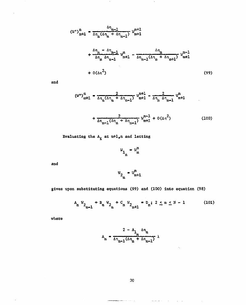
gives upon subst i tut ing equat ions (99) and (100) into equat ion (98)

A W + B W + C W2 = D * P < n L N - l 2n-1 2n n n+l n' -

where

30

and

A. w, + - [W; + A Wi + A2 W1 ] (1 X ) A3 4n 'n

Dn n 'n n n n n A-5

Assuming t h a t

W2 = E W n 2n+1 + Fn

is valid throughout the boundary-layer (Richtmyer [ref, 26]), then

w2 is given by ~ n-1

w2 = E W + Fnml n-1 n=l 2*

Using equation (103) in equa t ion (101) and solving for W2 and n

comparing with equation (102) gives !

and

31

The values of El and F1 are detemtned by the boundary condition

f o r W,

6.2,3 Spacing of Node P o i n t s i n t h e Normal Coordinate Direction

The-f ini te-difference solut ion procedure has been developed f o r a

var iable spacing of t h e node p o i n t s i n the normal (n) coordinate direc-

t ion. This permits a d08e spacing of poin ts in the region near She

wall where the va r i a t ion o€ € h i d and dynamic p rope r t i e s is grea te s t ,

The procedure employed I s tha t g iven by Cebeci, Smith, and Mosinskis

[ref. 121.

Using t h i s procedure, the ratio of the ad jacent in te rva ls is a

constant expressed as

k=- An*-l

The d i s t ance t o t he n th po in t measured from the wall boundary is

given by

where

N is the number of s t r i p s i n t he boundary-layer, and 0 i s the loca t ion

of t he boundary-layer outer edge, e

The values of the constant k for laminar or turbulent f low were

determined by numerical experiments. A number of so lu t ions were ob-

ta ined for laminar and turbulent boundary l aye r flows a t supersonic

32

condi t ions consider ing both adiabat ic and cold wall casee. The value

of k was varied over the range from 1 t o 1.5 with ne var ied from 4 t o

12 for laminar flow and from 75 t o 200 for tu rbulen t ' f low. The r e s u l t s

of these test cases were compared with experimental data to determine

a value of k which gave good agreement with experimental data and

where the so lu t ion showed l i t t l e change fo r d i f f e ren t va lues of ve.

The values selected were:

k m 1.04 and ne = 6 f o r laminar flow

k = 1.09 and ne 100 for turbulent: flow . " -

The above values correspond to a value of N = ZOO i n equa t ion (108).

Similar tests were made varying N from 50 t o 500. An N of 50 was

found t o b e u n s a t i s f a c t o r y f o r most cases, but values of N greater than

100 did not improve the so lu t ions which were obtained.

6.2.4 Convergence Criteria

A suitable convergence test may be es tab l i shed for l aminar

boundary-layer flows by comparing F; a t successive iterates of t h e

solut ion, This type of convergence test was employed by Davis [ref.

91 and Cebeci and Smith [ re f . 111.

For turbulent flaws, Cebeci and Smith found t h a t a second require-

ment based on successive iterates of the boundary-layer displacement

thickness was neceasa ry t o ob ta in s a t i s f ac to ry so lu t ions . They con-

t inued the i t e ra t fon procedure un t i l bo th tests were s a t i s f i e d .

For the present calculat ions provis ions were made t o e s t a b l i s h

convergence by comparison of successive iterates of both F; and g; o r

33

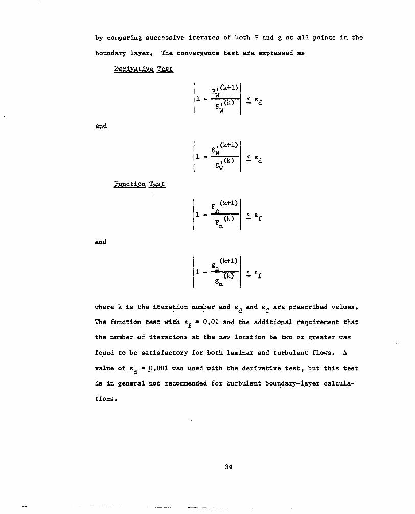
by comparing successive iterates of both F and g a t a l l po in t s i n t he

boundary layer , The convergence test are expressed as

and

Derivative -%

Function T e s t "

and

where k is t h e i t e r a t i o n number and cd and are prescribed values,

The function test with cf = 0.01 and the additional requirement that

t he number of i t e r a t i o n s a t the na7 location be two or grea te r was

found to be sa t i s fac tory for bo th l aminar and turbulent f lows, A

value of E - 0,001 was used with t he de r iva t ive test, b u t t h i s test

is i n general not recommended for tu rbulen t boundary-1,ayer calcula-

t ions

d

34

6.3 Speci f ica t ion of Body Geometry

The geometry of a given configuration is considered as a series

of segments of fourth order and requires that the coordinates , z , x,

and r be given i n t abu la r form, Since t ransverse-curvature effects

have been neglected i n the governing equations, provisions have not

been made t o d i s t i n g u i s h between d i f f e r e n t body sect ions. Thus, some

inaccuracies are introduced i n reg ions near the in te rsec t ion po in ts o f

different contours. For problems requir ing a spec i t ied p ressure

and/or a wall temperature dis t r ibut ion, these data are entered in tab-

ular forni a t the same po in t s as the geometry data. The temperature is

entered i n O R and the p ressure is given as P/Poor P/PA. 1

To insure accurate interpolat ion and/or different ia t ion of t h e

temperature and pressure da ta in reg ions of la rge g rad ien ts , it is nec-

essary to have a close spacing of the coordinate data.

For nozzles, a t least 30 points should be entered in the throat

region, and for b lunt bodies , a t least 50 points should be entered

for the nose eect ion. A maximum of 500 points may be tabulated, and

the minimum number permitted is 5 . Best r e s u l t s were obtained when

t h e maximum r a t i o of a d j a c e n t s t e p s i z e s i n z were not greater than

1.25.

The body shapes which have been considered are blunt bodies,

wedges, f l a t p l a t e s , and nozzles.

6.4 Fluid Proper t ies at the Outer Edge of the Boundary-Layer

I n t h e p r e s e n t method fo r so lv ing t he boundary-layer equations,

t h e e f f e c t s of mass entrainment of the outer inviscid vortical stream-

l i n e i n t o t h e expanding boundary-layer on a b lunt body is neglected.

35

Therefore, the edge conditions may be spec i f ied by conditions on the

body su r face fo r t he i nv i sc id f l a t of t he gas. The procedures em=

ploped fo r spec i fy ing t he outer edge conditions for t h e d i f f e r e n t geom-

etries and gas models is discussed in the fol lowing sect ions,

6.4.1 Axisvmmetric Nozzles

The edge conditions for nozzle flows of a per fec t or an equili- '

brim gas may be Specified by assuming a one-dimensional expansion or

t he expansion can be determined for a spec i f i ed p re s su re d i s t r ibu t ion

where the p ressure is given i n t a b u l a r form as ind ica t ed i n Sec t ion

6.3. The procedures employed for t h e d i f f e r e n t cases are discussed

below.

A. One-Dimensional Expansion of a Per fec t Gas

For a one-dimensional expansion of a perfect gas, tables of Mach

numbers and the rotresponding mea ratios are computed within the

bounhry-lapar mmpu%e5! program u s h g the relation

A/A, - 1 I4

at intervals of 0.03.in Mach number f o r M < 2 and i n intervals of 0.05

f o r M 2 2.

After the above cables' have been generated, the Hach number a t

the nozzle exit is determined by f ive po in t i n t e rpo la t ion i n the tables

of area r a t i o and Mach number with t he area r a t i o as the independent

36

variable, The exit Mach number is denoted by M,,

The free-stream pressure, temperature, velocity, density, vis-

cosity, and Reynolds number are then computed using the relations

rl *

m *

U, * M, /-

and

* P* pm - m

R G M T:

* + C

* *

* 312 Trefr

T, + c

* * * poa u m

'm

R - em

*

37

* * * where 'ref, , Tref, snd L are reference values of viscosity, temperature and length,

Corresponding to the points in the geometry arrays, tables of the

edge pressure and velocity are computed in nondimensionalized form

using the expressions

where

u e &To = Te)2

* * * * T c

r - r O p m TO TO To * *2 2 *

Tref L a (Y-1) M, T,

T I

0

Te 1 + * 2 2 %

and % is the local Mach number determined for the area ratio at the

given point in the geometry arrays.

At a local solution station x = x1 + Ax, Pe, ue and F$ are deter-

mined by interpolation, and Te, pe and p are computed using e

38

or

Te - To - ue/2 2

n L - 'e 'e y-1 Te

I- 1 +; 3/2 Te f 'E T€l

.(123)

where

* * 'e 'e

Pref p- 'e * I-=- *

and * 'e

'ref

I- 'e *

due The velocity derivative dx is evaluated numerically.

B. Pressure Distribution Specified for a Perfect Gas Solution

For solutions where the pressure distribution is input to the

computer program, the outer edge conditions are computed in the same

manner as for the one-dimensional expansion solution with the exception

that the Mach number table is computed from the input pressure distri-

bution using

39

After computing the Mach number array using equation (125 ) , equa-

t i ons (116)-(124) are evaluated using the local Mach number data cor- due responding to t he g iven p re s su re d i s t r ibu t ion , and - dx is evaluated

numerically.

C. One-Dimensional Expansion of a Reactinq

Gas i n Chemical Eauilibrium

-The boundary-layer edge conditions for the equilibrium gas case

were determined by the so lu t ion of the inviscid equat ions of motion

for the g iven-mixture of perfect gases. The da ta which must be given

f o r t h e boundary-layer so lu t ion are: \

These da ta are t abu la t ed fo r use with a table-look-up procedure. For

a one-dimensional expansion of t he gao mixture, the area r a t i o is used

as the independent variable to determine the local edge conditions for

the given body geometry. Since the area r a t i o is not a monotone func-

t ion over the length of the nozzle, i f was found t o . b e more satis-

f a c t o r y t o create a secondary expansion data set on a sc ra t ch un i t ex-

pressed in terms of z o r x. The loca t ions of z and x were determined

f o r a given A/A by in te rpola t ion and the secondary data set was writ-

t en as unformatted records in the order t

2, x, M, U , 3 and % *

This operation is performed within the boundary-layer program and re-

qui res no addi t ional preparat ion o€ the expansion data. In addition

40

t o t h e ex'pansion data tape, a tape un i t is requi red for the tables of

thermodynamic and transport properties of the equilibrium gas mixture.

These t ab le s are written a t constant 8 with the temperature decreasing,

The d a t a i n each table are wr i t t en as unfonnat ted records in the form

(P; T , h, p, l~ , cpD Pr). The expansion data and t h e tables of

thermodynamic and t ransport propert ' ies were obtained using two modified

versions of the computer program developed by Lordi et al. [ re f . 203.

* % % *

A descr ip t ion of these modif icat ions are given i n Appendix A,

After the secondary expansion data set has been wri t ten, local

values of M, U , P and % are determined by interpolation with either

z o r x as the independent variable. With the local values of 8 and h" as independent var iables , the local values of T , p, IJ , c and P r are

found by i n t e rpo la t ion i n t he t ab l e s of thermodynamic and t ranspor t

propert ies . The nozzle exit conditions are taken as the free-stream

conditions and the re fe rence condi t ions re ta in the same d e f i n i t i o n s i n

the dimensional form with the exception of uref. The reference vis-

*. 'L

* ' L * P

*

cos i ty for the equi l ibr ium cases may be chosen a r b i t r a r i l y and does

not necessarily correspond to the reference temperature and reference

pressure. The re ference v i scos i ty employed is computed using Suther-

land 's law.

D, EauiHbrium Gas Solut ions with the Pressure Distr ibut ion Given

I f t h e p r e s s u r e d i s t r i b u t i o n is given, the local value of P is 'L

determined by in t e rpo la t ion i n t he g iven p re s su re d i s t r ibu t ion table.

With t h i s v a l u e of 8 as the independent variable, local values of M, U and h are determined by interpolation of the data on the expansion * n4

41

data tape, It is not necessary for P t o be a monotone function, The

remaining edge conditions are determined by interpolation in the

tables of thermodynamic and transport properties with P and h as the

independent variables as in paragraph C above.

%

'I, %

6 .4 .2 Blunt - Bodies

The solution of the boundary-layer equations for flows over blunt

bodies requires that the pressure distribution be specified. The re-

maining edge conditions are determined for a perfect gas or an equili-

brium mixture of perfect gases as discussed below,

A. lsentrooic Expansion of a Perfect Gas Along

the Body 'Streamline From the Stagnation Point

For these solutions, the pressure distribution is entered in the

table a8 P/PA where PA .is the stagnation pressure behind a normal.

shock expressed in nondimensionalized form as

P:, - The reference conditions are based on the flow properties ahead of the

bow shock. Since the inviscid flow along the body streamline is isen-

tropic, the edge conditions are computed in the same way as for a noz-

zle with the pressure distribution given and is described in paragraph

C of Section 6.4.1 above. It is noted that the expansion is from the

stagnation conditions behind the normal shock.

42

B, Isentropic Expansion of an Equilibrium Gas

Along the Body Streamline from the Stagnat ion Point

For t h i s case, the equilibrium expansion data are determined f o r

the s tagnat ion pressure and temperature behind a normal shock f o r t h e

given mixture of perfect gases and free-stream conditions, The free-

stream and reference condi t ions with the except ion o f the re fe rence

v i scos i ty are determined by t h e f l u i d p r o p e r t i e s ahead of t h e bow

shock, The edge conditions at local points a long the body are deter-

mined i n t he same manner as for an equi l ibr ium so lu t ion for a nozzle

with the p ressure d i s t r ibu t ion g iven and is discussed i n 6,4,1 D,

6 , 4 , 3 Wedges and F l a t P l a t e s

The edge condi t ions for wedges and f l a t p l a t e s are constants cor=

responding to conditions behind an oblique shock or the free-stream

condi t ions respect ively. The computer program for the so lu t ion O€ t h e

boundary-layer equations is s u i t a b l e f o r b o t h wedges and f l a t p l a t e s

i f a perfect gas is considered, The so lu t ion of wedges for an equi l i -

brium gas requires modification of the boundary-layer computer program,

Thus, o n l y f l a t p l a t e s are considered for equt l ibr ium chemistry soh-

f ions , The procedure for determining the edge conditions for a per-

fec t gas and an equilibrium gas mixture is discussed below,

A, Edge Condit ions for Flat Plates snd

WedRes f o r a Per fec t Gas Solution

The pressure, temperature, and velocity a t t h e o u t e r edge of t h e

boundary-layer are computed from the obl ique shock re la t ions and are

expressed in nondimensional form by t h e r e l a t i o n s

43

2y M, 2 2 s in u - (y-1)

[2y M, s i n u - (y-1) J [(y=l) M, s i n cr + 2 J

Cy-1) .", (y+l) M, sin2 u

2 2 2 2

Te = 2 2 (127)

and

The dens i ty and v i scos i ty are computed using equations (122) and (123)

o r (124)

B, Flat-Plate Solutions for Equilibrium Gases

The so lu t ion of f l a t p l a t e s i n an equ i l ib r ium gas r equ i r e s t he

uae of the t ab l e s of thermodynamic and t r anspor t p rope r t i e s fo r t he

given gas mixture (Appendix A). The free-stream pressure, temperature,

and ve loc i ty are input da ta t o the boundary-layer computer program,

Using the free-stream pressure and temperature as independent vari-

ables, the va lues of h,, p,, p,, and c are determined by the use of * * * 2:

Pm i n t e r p o l a t i o n i n the t a b l e s of thermodynamic and t ranspor t p roper t ies ,

6.4.4 Evaluation of the Longitudinal Coordinate+

The coordinate 5 is evaluated by equation (26) numerically using

a modified Simpson's r u l e (Davis [ r e f . 9 ] ) , and is expressed a8

44

where t h e s u b s c r i p t s r e f e r t o t h e edge conditions a t the po in ts x

xm.+ 2 , and x $. Ax respect ively, .

m' Ax

m

6,.5 S o l u t i o n f o r t h e I n i t i a l P r o f i l e Data

The equations governing the laminar or turbulent boundary-layer

flow of a perfect gas or an equilibrium mixture of perfect gases

reduce to a system of ordinary non-l inear different ia l equat ions a t

x - 0 However, for ful ly developed turbulent flow, the eddy v i scos i ty

cannot be evaluated a t x = 0 , f o r f l a t p l a t e s or nozzles. The limit-

ing form of the d i f fe ren t ia l equa t ions are employed.at x = 0 fo r b lun t

body flows. The procedures used to ob ta in the s ta r t ing p rof i le da ta

are discussed belowr

6,S.l I n i t i a l P ro f i l e s fo r t he So lu t ion

of t he Laminar Boundary-Layer Equations

To s t a r t t h e s o l u t i o n of the boundary-layer equations, init ial

guesses of the profiles for the dependent variables F, g, and V are

required. A t the leading edge or s tagnat ion point , the equat ions are

ord inary d i f fe ren t ia l equa t ions , and t h e i n i t i a l p r o f i l e d a t a are

determined by an i terat ion procedure using the implici t f in i te -

45

di f fe rence scheme developed in 6.2.2,

I n i t i a l g u e s s e s are made f o r t h e p r o f i l e s and for t h e f i r s t itera-

t ion, These-est imates are denoted by t h e s u b s c r i p t s - ( )1 and (--- )c

respect ively and the k+l iterate is denoted by the subscr ip t ( )2 .

The i n i t i a l g u e s s e s of the p rof i le da ta a re .assumed to have the

forms given be lmt

a t 9 e ne at n - ne

F; - F" = - e -n

C F; - 0

The solu t ion of the cont inui ty equat ion is asaumed as

and the temperature dis t r ibut ion I s computed from the g pro f i l e u s ing

the def in i t i ons

8 . I -=- T h Te he

46

1 2 2

He he + ue 1 2 g r - r H h + T u e F

or

U 2

e + - - 1 e F 2 he

1 ue he

g = 2

1 +"

Solving for 8 gives

and

For a perfect gas

and the Chapman-Rubesin factor, C, Is assumed unity across the boundary=

layer

Using the above guesses of the profile data, the governing equa-

tions are solved to determine F2, F;, F;, g2, g;, and g" The sub-

scripted variables ( and ( >c are set equal.to the variables with 2'

47

subsc r ip t ( )2 and new values of 0, e', - 'e , Vc, and C are then

computed where P

vc = (25 FcE + PC) drl 0

C - A = &&. (Sutherland'e law) 'e "e (e + 3

o r

The procedure is r epea ted un t i l the convergence criteria of sec t ion

6.2.4 is s a t i s f i e d ,

For an equilibrium gas, t he i n i t i a l guesses of the profile data

are assumed t o be the prof i le data corresponding to the converged

s o l u t i o n f o r a perfect gas described above. Using the per fec t gas

p r o f i l e s of F and g, the remaining thermodynamic and t r anspor t prop-

erties are determined by use of the table-look-up procedure, Deri-

vatives of e and C are evaluated numerically for the equilibrium gas.

The i terat ion procedure is t he same as fo r t he pe r f ec t gas case.

6.5.2 I n i t i a l P r o f i l e s f o r t h e

Turbulent Boundary-Layer Eauations

The so lu t ion of f l a t p l a t e s , wedges, or nozzle flows assuming

fully developed turbulent f low assumes t h a t t h e p r o f i l e s a t x = 0 and

x = 0.001 are similar, This procedure has been adopted because the

48

values of E are zero a t x - 0. With this except ion and assuming an

i n i t i a l p r o f i l e f o r E as zero, t h e s tar t ing procedure is the same as

for the laminar boundary layer .

+ +

An a l t e r n a t e method fo r s t a r t i ng t hese so lu t ions is t o use t he

l a m i n a r s t a r t i n g p r o f i l e at x - 0 and assume an instantanequs t ransi-

t i on t o t u rbu len t f l ow a t x > 0.001, Both methods have been used and

t h e d i f f e r e n c e s i n t h e r e s u l t i n g s o l u t i o n s are ins ign i f i can t .

For b lunt body so lu t ions , t he t u rbu len t s t a r t i ng p ro f i l e s are

determined a t x - 0 us ing the l imi t ing form of the governing equations.

The i n i t i a l g u e s s e s of t h e s t a r t i n g p r o f i l e s f o r t h e e q u i l i b r i u m

so lu t ion is determined from t h e converged p r o f i l e s f o r a perfect gas.

Using. these prof i les , the i terat ion procedure is continued using the

equilibrium gas properties unt5l the convergence tests are s a t i s f i e d . - . _ .

6.6 Boundary-Layer Paramaters

The de f in i t i ons of t he boundary-layer thicknesses, skin-friction

coef f ic ien t , hea t t ransfer , hea t t ransfer coef f ic ien ts , and Stanton

numbers which have been used i n t h e boundary-layer calculations are

presented in t h i s s e c t i o n . Both the dimensional and nondimensional

expressions are given,

Velocity o r Boundary-Layer Thickness

U * * ‘ I =

The veloci ty thickness , 6, is assumed t o b e t h e v a l u e of y a t

0.995, and is determined by i n t e r p o l a t i o n i n t h e v e l o c i t y p r o f i l e

*

U e a r ray

Incompressible Displacement Thickness

The incompreasible displacement thickness is computed us ing the

49

L

two-dimensional definition

* 6; - T'

0

[I - 4 dr*

or

Compressible Displacement Thickness

Two-dimensional

* b*"

0

or

50

. . " ~~

Axiepmmetric t

The axiaymmetric compressible displacement: thickness is approxi-

mated arr; (Cebeci and Moeinskia- [ref. 271): " - -.- .

* *

* r

or

Momentum Thickness : ..

*

or

Heat Transfer Ratet

In dimensional variables

51

or

In nondimensional f o m

'.*

or in Levy-Lees variables

j 'e 'w He 'e ue ' R " ' prW [%I W

k is converted t o BTU/ft2-aec as

'* * *3 R gW 'ref Uref 'VD /778

Film Coefficients:

** * c"

BTU/ln -sec-'R 2 h g l = * *

Hw - HAtr (778) (144)

or

i * * *

52

a 32.17 lbm/in -sec * * 144 2

cHw HAw)

or

b * * % “VD ’ref Uref 32.17 lbm/in -sec 2

hg2 a (Hw - HAW) 144

Stanton Number Definitions:

A, Based on free-stream conditions

% St, = - * * * * p, U- (He - Hw)

or

B , Based on edge conditions

’* % Ste = - * * * *

p, ue (He - Hw) or

s, Ste - - p, ue (He - Hw) Heat Tranefer Coefficients:

A. Based on free-stream conditions

53

'* I- 9,

%? * * * * p, U- (HAW - Hw)

or

B. Based on edge conditions

'*

or

Skin-Friction Coefficients:

A. Based on free-stream conditions

or

B, Based on edge conditions:

* ?W

e 'e ue cf

P" * *2

54

or

cf , Cf - -

e PC? ue 2

55

VII. RESULTS AND DISCUSSION

The impl ic i t f in i te -d i f fe rence scheme developed i n Chapter V I has

been appl ied to obtain solut ions of laminar and turbulent boundary-

layer f lows of perfect gases and equi l ibr ium gas mixtures over f la t

p la tes , an hyperboloid, a spherically blunted cone, and i n axiaym-

metric nozzles.

Solutions of perfect gas turbulent; f lows using different expres-

s ions fo r ' t he i nne r eddy v i scos i ty law are presented in Sect ion 7.1,

and are compared with experimental data and/or other numerical solu-

t i ons €or cases where these data were available. Solut ions using the

equilibrium gas option are presented in Sect ion 7.2, and the so lu t ion

of boundary-layer flows with mass i n j ec t ion are presented in Sect ion

7.3.

The numerical solutions presented assume e i t h e r f u l l y developed

turbulent o r laminar flow; however the boundary-layer computer pro-

gram described by Miner, Anderson, and Lewis [ r e f , 281 provides

opt ions €or e i t h e r an instantaneous or a cont inuous t ransi t ion from

laminar to t u rbu len t flow. The cont inuous t ransi t ion model is based

on the exper imenta l resu l t s of Owen [ r e f . 291 and is d iscussed in the

repor t on t h e computer program.

7.1 Per fec t Gas Turbulent Boundarv-Layer Flows

Solut ions of turbulent f lows over f la t p la tes and i n axisymmetric

nozzles using the inner eddy v i scos i ty laws of Van Driest, equation

(70). Cebeci and Smj.th, equation (721, absolute value of the pressure

gradient, equation (73), and Reichardt, equation (77), are presented

56

. " -

i n t h i s s e c t i o n . The inner eddy v i s c o s i t y law proposed by Patankar

and Spalding, equation (731, was found t o be unsat isfactory for f lows

having a s igni f icant favorable p ressure g rad ien t and is nor; considered.

7.1.1. Perfpct Gas_S.olu.tions for Turbulent Flows Over F l a t P l a t e s

For f la t -p la te f lows the inner eddy v i scos i ty laws expressed by

equations (70)-(74) are i d e n t i c a l and are r e f e r r e d t o as t h e Van

Drieet model. The inner eddy v i scos i ty law given by equation (77) is

r e f e r r e d t o as the Reichardt model,

Three f la t -plate solut ions are presented corresponding to case

numbers 20, 26, and 62 of the experimental data given by Coles [ref.

301. The r e s u l t s of the present numerical method of so lu t ion are

compared with Coles' experimental data and the so lu t ions of Van Driest

[ re f . 221 and Dorrance [ref. 311. The free-s t ream condi t ions for the

th ree cases are given in Table I. The free-stream Mach numbers f o r . .

casea 20, 26, and 62 were 3,701, 2,578, and 4.544 respect ively, and

the p l a t e s were assumed to be ad iaba t i c .

Boundary-layer displacement thicknesses predicted using the Van

Driest: and Reichardt eddy v i scos i ty models are compared with Coles'

exper imenta l da ta in F igure 2. The displacement thickness predicted

us ing the Van Driest and Reichardt eddy v i scos i ty model were found t o

d i f f e r by less than 3% f o r t h e t h r e e cases, but the predicted values

of displacement thickness differ from Coles' experimental data by as

much as 20X. The numerically determined displacement thickness is l e a s

than the experimental value in a l l t h r e e cases. The numerical resul t

is i n good agreement with experiment for Case 62.

57

The numericalxy determined velocity profiles a t x = 21.48 i n , f o r

Case 20 are presented i n F i g u r e s 3 and 4. The r e su l t s u s ing e i the r

eddy v i scos i ty model are i n good agreement with Coles' experimental

data. Figure 4 shows the solut ion given by Van Driest [ r e f . 221.

Figure 5 shows t h e eddy v iscos i ty p rof i les p red ic ted us ing the Van

Driest and Reichardt eddy v i scos i ty models a t x - 21.48. The d i f -

f e r e n c e i n t h e two models is no t s ign i f i can t .

The predic ted sk in- f r ic t ion coef f ic ien ts for the th ree cases are

compared wi th t he so lu t ion of Dorrance [ref. 311 and Coles' experi-

mental data in Figure 6 . The sk in - f r i c t ion p red ic t ions fo r Cases 20

and 26 are i n excellent agreement.with both the experimental data and

Dorrance's solutions, For Case 62, the present method of so lu t ion is

i n good agreement with the experimental data points for Reynolds num-

bers g rea te r than 3 x lo6, b u t f o r Re, = 1.7 x 10 the present numer-

ical so lu t ion pred ic t s a sk in- f r ic t ion coef f ic ien t which i s approxi-

mately 15% lower than the experimental value. The present method of

so lu t ion is i n b e t t e r agreement with the experimental data for this

case than the solution of Dorrance.

6

The above r e s u l t s are representa t ive examples of t u rbu len t f l a t -

p l a t e so lu t ions and i n a l l cases considered the numerical results were

not s ignif icant ly inf luenced by the choice of the inner eddy v i scos i ty

law. However, the use of the Reichardt inner law reduced the comput-

ing time by a f a c t o r of approximately 10 (see Section 7.1.3).

7.1.2 Turbulent Flow o f - P e r f e c t Gases i n Axismetric Nozzles

The present method of solution has been used to so lve t h ree axisym-

metric nozzles, and the results are compared wi th the in tegra l method

58

of so lu t ion developed by Elliott, Bartz, and Silver [ r e f , 151 and ex-

perimental data where t h e data were ava i lab le , The inner eddy vis-

cos i ty laws of Van Driest, equation ( t o ) , Cebeci and Smith, equation

(72), absolute value of the pressure gradient, equation (73), and

Reichardt, equation (771, have been considered for the sample case

given by E l l i o t t , Bartz, and Silver [ r e f , 151,

A, El l io t t , Ba r t z , and Silver Sample Case

The problem conesdered cons i s t s of a 30’ con ica l i n l e t s ec t ion , a

c i r c u l a r arc throa t sec t ion wi th a throa t rad ius of 0,885 i n , and a

15’ conical d ivergent sect ion, The reservoi r p ressure and temperature

were 300 p s i a and 4500’R respec t ive ly , The s p e c i f i c h e a t r a t i o , y,

was assumed t o be 1,2 and t h e wall temperature was assumed t o be a

constant; value of 1145’R, The d a t a f o r t h i s case are given in Table

11, and the nozzle geometry is shown i n F igu re 7,

Eddy v iscos i ty p rof i les p red ic ted a t the nozzle throat using the

€our eddy v i scos i ty models are shown i n F i g u r e 8. In t he r eg ion nea r

t h e wall, n < 0,4, the eddy viscosi ty predicted using the four inner

laws are e s s e n t i a l l y i d e n t i c a l , The Cebeci and Smith inner law (72)

pred ic t s a gecond zero value of E: a t II = 1,2 result ing from the pres- +

sure gradient tam y/p being equal and opposite i n s i g n to ‘cw/p,

It is noted t h a t the solution using the Patankar and Spalding expres-

sion, equation (71), fails upstream of the throat: as a r e s u l t o f t h e

square root: term being negative, By replacing the aum

dP

59

Cebeci and Smith [ref. 111 were success fu l i n ob ta in ing so lu t ions t o

problems having a s igni f icant p ressure g rad ien t . This model, equation

(72), r e s u l t s i n s u b s t a n t i a l l y smaller values of c+ f o r most of the'

boundary-layer than is given by the Van Driest Law, equation (70), t he

absolute value of the pressure gradient equat ion (73) and the Reichardt

Law, equation (77) . The values of E' corresponding to the Van Driest

expression and the expression using the absolute value of the pressure

g rad ien t d i f f e r by less than 3%, and the E+ corresponding to the outer

law, equation (79) , II > 1 r 7, a l s o d i f f ets by less than 3%. I n t h e

sublayer, the Reichardt expression, equation (77), predicts values of

E* which are 1 0 t o 20% larger than those given by equations (70) and

(73), but above the match point with the outer law, 0 = 1.4, c+ is

near ly the same as when using equation (70) or equation (73) f o r t h e

inner law. It is emphasized t h a t t h e o u t e r eddy v i scos i ty law is t h e

same express ion in a l l cases,

The resu l t ing p rof i les o f ve loc i ty and temperature differed by

less than 5% for the so lu t ions ob ta ined us ing the d i f fe ren t v i scos i ty

lawsr The boundary-layer paramaters 6 , 6 , 0 , cf , etc. also agreed

to w i th in 54. I f t he i nne r law of Cebeci and Smith is excluded i n t h e

* aD

comparison, the resu l t ing so lu t ions d i f fe red by less than 3%. These

resu l t s ind ica te tha t inc luding the p ressure g rad ien t term in the inner

law had l i t t l e inf luence upon the eddy v i scos i ty p ro f i l e s , and had

60

e s s e n t i a l l y no inf luence upon the resu l t ing so lu t ion .

As a r e s u l t of t h e above, and the formulations of equations (71)

and (72) fo r t he i nne r law, these expressions were dropped from fu r the r

consideration. The r e s u l t s which are discussed below were obtained

using the Van Driest or Reichardt expression for the inner eddy vis-

cos i ty law. However, as in the previous cases, use of the Reichardt

inner law resu l ted in a substant ia l reduct ion of the computer time re=

quirement (see Section 7.1.3). S ince the d i f fe rences in these so lu-

t i o n s were i n s ign i f i can t , t hese da t a are shown as a s ing le curve.

The heat t ransfer coeff ic ient , bouadary-layer , momentum, and dis-

placement thicknesses predicted by the present numerical solut ions are

compared i n Figures 9-12 with the resu l t s ob ta ined by El l io t t , Ba r t z ,

and S i lve r [ r e f . 151 us ing an in tegra l method of solut ion, The solu-

t ions using the present numerical method and t h e i n t e g r a l method d i f f e r

by up t o 30%; however it should be noted, that the solut ions using the

i n t e g r a l method can be varied over a wide range by changing t h e assump-

t i ons which must be made r e l a t i n g t o t h e nominal entrance conditions.

S ince t he s t a r t i ng p ro f i l e s fo r t he p re sen t method are determined from

the so lu t ion of the governing equations, direct comparison of t he two

methods is not possible, a l so i t is not clear what assumptions should

be made f o r t h e i n i t i a l c o n d i t i o n s necessary f o r t h e i n t e g r a l method

i f exper imenta l da ta were not: ava i lab le before the ca lcu la t ions are

made. Because of the a rb i t ra r iness o f the so lu t ion us ing the in tegra l

method, t h e agreement of t h e two solution procedures is considered. to

be adequate,

61

B. NASA-Lewis Case 2a (Boldrnan et al. [ref. 161)

The nozz le conf igura t ion cons is t of a 30" conical convergent sec=

t ion , a c i r c u l a r arc throa t sec t ion , and a 15" conical divergent sec-

tion. The throa t rad ius is 0.746 in., and the s tagnat ion pressure and

temperature were 300 ps ia and 970"R respectively. The test conditions

are g iven i n Table 111. The geometry is shown i n F i g u r e 13, and the

pressure distribution corresponding to a one-dimensional expansion and

the experimental data are shown i n Figure 14. The experimentally

determined wall tempera ture d i s t r ibu t ion is shown i n Figure 15.

So lu t ions t o t h i s problem were obtained using the Van Driest and

the Reichardt expressions, equations (70) and (77), fo r t he i nne r eddy

v i scos i ty laws, and as in t he p rev ious ly d i scussed E l l io t t , Ba r t z , and

S i lve r sample case, the d i f f e rences i n t he so lu t ions were ins ignf f i -

cant. However, the so lu t ion us ing the Van Driest inner law required

approximately 10 times more computing time than was necessary using

the Reichardt inner law (see Section 7.1.3).

The predic ted hea t - t ransfer coef f ic ien t us ing the p resent method

of solution i s compared with the experimental data and the so lu t ions

obtained using the El l iot t , Bartz , and S i l v e r i n t e g r a l method in F igu re

16. The present method of so lu t ion is i n e x c e l l e n t agreement with the

experimental data in the throat region and downstream. Differences of

up t o 20% between the p red ic ted and experimentally determined heat-

t r ans fe r coe f f i c i en t are noted in t he subson ic r eg ion of the nozzle.

The near discontinuous change in the experimental value of the heat-

t r ans fe r coe f f i c i en t a t z = 1.97 is the resul t of the temperature tabu-

l a t e d in t h i s r eg ion (see Figure 15), and also the experimental pres-

su re da t a were not smooth in t h i s r eg ion . For the present calculat ions,

62

these da ta were smoothed i n the region 1.9 z 5 2.5. The i n t e g r a l

method of so lu t ion is s e e n t o r e f l e c t a strong dependence upon the

s t a r t i ng cond i t ion asoumptions. The two solut ions presented using the

i n t e g r a l method d i f f e r from each other by as much as 50%.

C. AEDC Hotshot Whd Tunnel Nozzle

The problem considered corresponds t o t h e case r e f e r r e d t o as

"Hotshot 1" by EdenLield [ r e f , 171. The nozzle geometry, wall enthalpy

and pres su re d i s t r ibu t ion are shown i n F igu res 17-19, The operating

conditions are given in Table I V , In th i s s ec t ion t he expe r imen ta l

p reesure d i s t r ibu t ion ahown i n Figure 19 was not used, The r e s u l t s

presented assume a one-dimensional axpansion of nitrogen.and the speci-

f i c h e a t ratio, y, was taken as 1.4. The experimental wall enthalpy

d is t r ibu t ion , F igure 18, f o r 20 milliseconds of tunnel operat ion was

used, The s tagnat ion pressure and temperature were 11,500 p s i and

5400"R. The nozz le cons is t of loo and 5' converging conical in le t

sect ions, a f a i r e d ci-rcular arc throa t sec t ion , and a 5 O conical d i -

vergent section. The throa t rad ius is 0.055 in.

Attempts t o s o l v e t h i s problem using the Van Driest expression,

equation (70), for the inner eddy v i s c o s i t y r e s u l t e d i n a n i n s t a b i l i t y

a t z / r = loo,* When the Reichardt inner eddy v i scos i ty law, equation

(77). was used a complete solution was obtained. The so lu t ions ob-

ta ined are compared for va lues o f z / r up t o 100 i n F i g u r e s 20-23.

*

*

Figure 20 shows t h e eddy v i s c o s i t y p r o f i l e s f o r z / r i n t h e r a n g e *

from 7 t o 80, Dif fe rences i n t he eddy v iscos i ty us ing the two models

*This applies only i f t h e v e l o c i t y d e r i v a t i v e i n e q u a t i o n (70) is evaluated implici t ly (see Section 7.1.3).

63

d i f f e r from 5 t o 20X with the larger differences being a t s t a t ions nea r

the nozzle throat. Heat-transfer rates predicted using the two eddy

v i scos i ty models are s h a m i n Figure 21. For t h i s problem, the Van

Driest inner law resu l ted i n heat- t ransfer rates which are approximately

10% higher than the predicted heat ing rates using the Reichardt inner

law in the reg ion near and upstream of the throat. Downstream of the

th ros t , t he Van Driest model oscil lated about the solution obtained

using the Reichardt inner eddy v i scos i ty law. The displacement thick-

ness predict ions using the two inner eddy v iacos i ty laws were near ly

i d e n t i c a l and are shown i n Figure 22.

The computer t ime required to obtain a s o l u t i o n t o a given axial *

posi t ion, z / r , i s shown i n F i g u r e 23. The c u r v e s i l l u s t r a t e t h e time

requirement i n terms of the t o t81 number of i t e r a t ions . The use of

t h e Van Driest inner law required approximately f ive times as many

i t e r a t i o n s t o o b t a i n 8 so lu t ion to z / r - 100 as was necessary for the

complete solution using the Reichardt inner law.*

*

The problems discussed i n t h i s section have demonstrated that the

choice of the inner eddy v i scos i ty law Bad l i t t l e inf luence upon the

r e s u l t i n g s o l u t i o n f o r cases where convergence was obtained, and t h a t

the computing time requirement was considerably less when the Reichardt

expression was used for the inner law (see Section 7.1.3). For the

cases where experimental data were ava i l ab le , t he r e su l t s ob ta ined w i th

the p resent method of so lu t ion were i n good agreement with these data.

*This app l i e s on ly i f t he ve loc i ty de r iva t ive i n equa t ion (70) is evaluated implici t ly (see Sect ion 7.1.3).

64

7.1.3 Revised Evaluation of the Inner Eddy Viscosity Laws

Af te r the so lu t ions d i scussed in Sec t ion 7.1 and 7.2 were ob-

ta ined , the more recent expression for the inner eddy v i scos i ty law

given by Cebeci [ r e f . 131 became ava i lab le , T h i s re la t ion, equat ion

(74), was used i n t h e boundary-layer computer program with and without

including the preasure gradient term; equation (74) i s t h e same as

that g iven by Van Driest, equation (70). when the p ressure g rad ien t

term is neglected. The resu l t s ob ta ined using equation (74) with the

pressure gradient term included were e s s e n t i a l l y t h e same as that g iven

by t h e Van Driest expression and r e su l t ed i n i n s t a b i l i t y a t z / r = 100

for t he AEDC nozzle.

*

I n a l l of t h e r e s u l t s which have been presented up t o t h i s p o i n t

using Van Driest's and Cebeci ' s expressions for the inner eddy vis-

cos i ty , the ve loc i ty der iva t ive was e v a l u a t e d a t . t h e s t a t i o n x + Ax. It was noted that i n the cases which r e s u l t e d i n converged solut ions,

the solut ions obtained were relat ively unaffected by the i nne r eddy

v i scos i ty law which was used, and that: a l a r g e number of i t e r a t i o n s

were necessary i f v i s c o s i t y laws based on Van Driest's [ r e f . 221 modi-

fication of Prandtl 's mixing length were used. The diff icul ty appeared

t o be in the evaluat ion of To determine t h e inf luence of the

impl ic i t eva lua t ion of the veloci ty der ivat ive, the approximation (%)x+*x

was made. With th i s replacement, the Van Driest inner law, equation

(70), r e su l t ed i n so lu t ions which were e s s e n t i a l l y i d e n t i c a l t o t h e

65

solut ions obtained using the Reichardt expression, equation ( 7 7 ) , and

the computer time requirement was nea r ly t he same for both eddy vis-

c o s i t y laws. When the pressure gradtent was included in equat ion ( 7 4 ) ,

t he r e su l t s ob ta ined showed tha t the p ressure g rad ien t term had l i t t l e

inf luence upon the solut ion. For the cases considered, the use of

equations (70), ( 7 4 ) , and ( 7 7 ) r e su l t ed i n so lu t ions which agreed t o

wi th in 2 3%. Therefore , the resu l t s comparing the eddy v i scos i ty laws

presented in Sect ion 7.1 should be considered as the in f luence of t he

i m p l i c i t evaluation of - ra ther than the d i f fe rences i n the eddy vis-

cosity expressions.

aF a n

The results presented in ' Section 7.2 have been obtained uaing the

Reichardt expression for the inner eddy viscoai ty , and as mentioned

above, the so lu t ions are not s ign i f icant ly a f fec ted by the choice of

the inner eddy viscosity expression. Equations (71) and ( 7 2 ) were not

cons idered in th i s eva lua t ion .

7 .2 Laminar and Turbulent Boundary-Layer Flows of Reacting Gas

Mixtures i n Chemical Equilibrium

For the perfect gas solut ions presented in Section 7.1, i t was

possible to obtain experimental data for most of t h e problems con-

sidered. However, it has not been possible to obtain experimental data

in the range of pressure and/or temperature where the departure from

the perfect gas condi t ion is s igni f icant . For the problems considered

in th i s sec t ion , bo th the per fec t and the equi l ibr ium gas solut ions

are given for the cases where s ign i f icant d i f fe rences were found t o '

exist:

To check the accuracy of t he table-look-up procedure, a number of

66

problems were solved a t conditions corresponding to the range of pres-

Sure and temperature where the perfect gas re la t ions are correct . For

t h e cases considered the solutions with the table-look-up and the per-

f e c t gas optione agreed to within 5 3Z.

7.2.1 Equilibrium Gas Solu t ions for

Laminar and Turbulent Flows Over F l a t P l a t e s

ltro f l a t p l a t e cases were considered corresponding to the experi-

mental data given by Hironimus [ re f . 321. The free-stream Mach number

and temperature for Case 1 were 7.391 and 533"R and f o r Case 2, were

7.58 and 339"R respect ively. The wall temperature was 533'R f o r Case

1 and 355"R f o r Case 2. The test conditions are g iven in Table V.

P l o t s of Stanton number based on edge conditions are shown for bo th

f u l l y developed turbulent and laminar flow for Case 1 and Case 2 i n

Figures 24 and 25. The so lu t ions shown were obtained with the table-

look-up procedure. The per fec t gas so lu t ions for these cases d i f fe red

from the equi l ibr ium solut ion by less than 3% and are not presented.

Downstream of t h e t r a n s i t i o n from laminar to turbulent f low the

agreement of the predicted and the experimentally determined Stanton

number da t a is wi th in lo%, and i n the region of laminar flow the agree-

ment between the numerical and experimental data is good.

7,2.2 Equilibrium and Per fec t Gas Solu t ions for

Laminar Flow Over a Hyperboloid

A 10" half-angle hyperboloid a t a n a l t i t u d e of 100,000 f t . with

a wall temperature of 1400°K was considered for a free-stream Mach

number and temperature of 20.178 and 226.98"K. This case corresponds

67

t o Case A of t h e AGARD test cases (Lewis [ re f . 331) . The f l i g h t con-

d i t i ons are given i n Table V I . The body geometry and p res su re d i s t r i -

but ion are shown i n Figures 26 and 27.

The so lu t ions of bo th per fec t a i r and equilibrium air have been

obtained for the laminar case only. The per fec t gas so lu t ion is com-

pared with the results of Adam [ref . 341, and the equilibrium solu-

t i o n is compared wi th Blo t tner ' s and Smith's r e s u l t s as presented by

Lewis [ re f . 331 . Figure 28 shows the boundary-layer displacement thickness pre-

d i c t ions fo r t he pe r f ec t and equilibrium air cases. The present method

of so lu t ion is s e e n t o b e i n e x c e l l e n t agreement with Adams' so lu t ion

fo r t he pe r f ec t gas case. The present equilibrium air s o l u t i o n l e i n

good agreement with the results given by Keltner and Smith [ r e f . 351

but d i f fe rs by a f ac to r of two from the solut ion given by Blot tner

[ re f . 11. It is noted tha t Blo t tner used f in i te rate chemical re-

act ions and complete multi-component diffusion whereas Keltner and

Smith used 8 f inf te - ra te b inary a i r model.

P lo t s of the sk in- f r ic t ion coef f ic ien t and Stanton number d i s t r i -

but ions are shown in Figures 29 and 30. For the per fec t gas case the

skin f r ic t ion p red ic ted by the present method of so lu t ion is i n excel-

l e n t agreement with Adams' so lu t ion fo r S / r > 0.4, bu t t he so lu t ions

d i f f e r by up t o 10% near . the s tagnat ion point . The Stanton number

dis t r ibut ion given by the present method is i n good agreement with

Adams' r e s u l t s f o r a l l S/rn.

n -

For the equi l ibr ium air solut ion, the present method is i n excel-

l e n t agreement with Blottner 's solution for both skin-friction and

68

Stanton number d i s t r ibu t ions .

The maximum di f fe rences between Blot tner 's , Keltner and Smith's,

and the present results are less than 5%.

7.2.3 Equilibrium and Per fec t Gas Solu t ions for Laminar and

Turbulent Flow Over a Spherically-Blunted Cone

A 5' half-angle spherically-blunted cone a t a n a l t i t u d e of 70,000

f t , is considered i n th i s sec t ion .* The free-stream Mach number and

temperature were 19,564 and 226.98"K respect ively. The wall tempera-

t u r e was assumed to be cons t an t a t 1000°R. The problem da ta are pre-

sented in Table VII. The geometry and p res su re d i s t r ibu t ion are shown

in F igures 31 and 32, The p r e s s u r e d i s t r i b u t i o n f o r t h i s case was

determined f o r p e r f e c t air , y - 1.4, using t he computer program devel-

oped by Inouye, Rakich, and Lomax [ref . 361.

This problem is included t o i l l u s t r a t e t h e s o l u t i o n of a weak

adverse p ressure g rad ien t resu l t ing from an overexpansion and recom-

pression of the gas. Solutions are given for both laminar and f u l l y

developed turbulent f low for specif ic heat ra t ios , y, of 1.4 and 1.165

and equilibrium air.

The boundary-layer displacement thickness, skin-friction, Stanton

number, and heat- t ransfer rate d i s t r ibu t ions fo r t hese so lu t ions are

presented in Figures 33-37. Since experimental data or other numerical

so lu t ions are not: ava i l ab le for comparison, it is n o t p o s s i b l e t o

assess the accuracy of the resul ts . However, because of t h e s i m i l a r i t y

*This case was provided by Mr. Randy Graves of the NASA Langley Research Center as representat ive of a body of unpublished free-flight experimental data a v a i l a b l e f o r t h i s body.

69

with the hyperboloid discussed in Sect ion 7.2.2, these resu l t s appear

t o show the cor rec t t rends .

7.2.4 Turbulent Flow of Equilibrium Gases in Axisyrmnetric Nozzles

"he d a t a f o r t h i s case are g iven in Sec t ion 7.1.2.C of t h i s

Chapter. Edenfield [ref. 171 considered the nozzle discussed i n t h i s

sect ion for prel iminary invest igat ions leading to the design of con-

toured nozzles for hypersonic hotshot wind tunnels with a test sec-

t i o n Mach number of about 20. Edenfield used a number of theor ies to

pred ic t the downstream boundary-layer displacement thickness, but the

ava i l ab le methods of p r e d i c t i o n e i t h e r f a i l e d t o g i v e a complete solu-

t i on fo r t he nozz le or t h e r e s u l t s were found t o be unacceptable.

Attempts t o s o l v e t h e problem us ing the E l l io t t , Bar tz , and S i lve r

[ re f . 151 i n t e g r a l method f a i l e d a t z / r = 1350.* T h i s f a i l u r e was

a t t r i b u t e d t o t h e assumed power Law to ta l en tha lpy p ro f i l e s used i n t h e

i n t e g r a l method. All other a t tempts t o predict the displacement thick-

ness used the momentum equat ion only with the Crocco enthalpy dis t r ibu-

t ion or correlat ion formulas .

*

Before discussion of the present resul ts , a br ie f descr ip t ion of

the physical nozzle contour and the contour used in the calculat ions

is given. The physical nozzle consis ts of a subsonic region composed

of a 10' conical section followed by a 5' conical sect ion. The th roa t

i s cy l indr ica l wi th a length of one throat diameter and the supersonic

port ion is a 5' conic sect ion. For the calculat ions, the nozzle con-

tour was smoothed as shown in F igu re 17 ,

*In t h i s s e c t i o n r denotes the non-dimensional throat redius . *

70

It should also be noted tha t t h e t o t a l l e n g t h of the nozzle was

given as 92,087 inches (Menfield [ref. 171, Using a th roa t r ad ius of

0,055 inches r e su l t s in a maximum value of z / r of approximately 1684,

However, experimental pressure measurements are g iven in F igure 19 f o r

values of z/r up to approximately 1850. The pressure data used up-

stream of z / r = 100 corresponds to an isentropic expansion of t h e

gas (nitrogen) a The t r a n s i t i o n from the isentropic expansion pressure

d a t a t o the experimental data is p a r t i c u l a r l y n o t i c e a b l e i n t h e l a r g e r

scale p lo t s o f t he boundary-layer thicknesses computed using the pre-

s en t method o f so lu t ion fo r z / r between 100 and 400. With reference

t o t h e above comments, i t is not clear what conclusions should be

made i n t h e comparison of the p red ic ted and experimental.disp1acement

thickness, However, t he same conditions have been used for a l l pre-

d i c t ion methods and t h e r e s u l t s of t he d i f f e ren t so lu t ions may be

compared,

*

* *

*

The momentum th i ckness d i s t r ibu t ion co r re spond ing t o t he E l l i o t t ,

Bartz, and S i l v e r i n t e g r a l method o f so lu t ion and the present method

is shown i n F i g u r e 38. The v e l o c i t y o r boundary-layer and displacement

thickness are shown i n F i g u r e 39, and the predicted heat- t ransfer rates

are g iven in F igure 40, The resu l t s p resented in F igure 40 from t h e

i n t e g r a l method were obtained by so lv ing bo th the momentum and energy

equations with a power law f o r the to ta l en tha lpy prof i les .

The d i f fe rences i n t h e boundary-layer thickness predictions vary

from 10% f o r t h e v e l o c i t y t h i c k n e s s t o a fac tor o f 2 f o r t h e momentum

and displacement thicknesses, The heat- t ransfer rates predicted by t h e

i n t e g r a l method are from 30 t o 60% lower than the rates predicted by

71

the present method. The results obtained with the integral , method do

not appear to be realistic, and as noted previously the method f a i l e d

a t z / r = 1350. The assumed power law to ta l en tha lpy prof i les to -

ge ther wi th the assumed v e l o c i t y p r o f i l e s i n t h e i n t e g r a l method

r e s u l t e d i n s o l u t i o n s which predic ted l a rge dens i t ies near the ou ter

edge of the boundary layer i n t h e downstream region of the nozzle.

The dens i ty p rof i les p red ic ted by the i n t eg ra l method, t he method of

Enkenhus and Maher [ r e f . 371 using the Crocco enthalpy dis t r ibut ion,

and the present method are shown i n F i g u r e 4 1 f o r z / r = 984. As

noted by Edenfield [ref. 171, p i to t p re s su re measurements would de tec t

the presence of these peaks in dens i ty if they exist, but the measure-

ments made indicate that such peaks do not ex is t . The d e n s i t y p r o f i l e

predicted with the present method shows a decrease in dens i ty near the

wall which is c h a r a c t e r i s t i c of boundary l aye r s fo r co ld wall cases.

*

*

Figure 42 shows the boundary-layer displacement thickness pre-

d ic ted by Enkenhus and Maher [ re f . 371, Burke and Bird [ ref . 381, Lee

[ref. 391, El l io t t , Bar tz , and Silver [ re f . 151, and the present

method of solut ion. The present two-dimensional displacement thick-

ness predict ion i e i n g e n e r a l agreement with Burke's calculation based

on t h e edge Reynolds number. The axisymmetric value of the displace-

ment-thickness prediction is i n g e n e r a l agreement with the solution

of Lee. Burke's solution based on a reference Reynolds number ( the

reference Reynolds number is computed using Eckert 's reference condi-

tions) gave the best agreement with the date presented near the nozzle

ex i t , bu t as noted a t the beginning of this eect ion, the experimental

data presented a t z / t = 1825 is outside of the nozzle dimensions. *

72

The methods of Enkenhus and Maher, and El l io t t ; Bar tz , and Silver are

i n poor agreement with the experimental data presented and the o ther

solut ions.

Figure 43 shows the displacement thickness predictions of t h e

E l l io t t , Ba r t z , and S i lve r method fo r bo th an assumed power law and the

Crocco enthslpy dis t r ibut ion. For the Crocco en tha lpy d i s t r ibu t ion

only the momentum equation is solved by t h e i n t e g r a l method. Two solu-

t ions are given corresponding to different skin-fr ic t ion laws using the

method of Enkenhus and Maher. The present two-dimensional and axisym-

metric so lu t ions are i n good agreement with the other solution proce-

dures which use the momentum equation only. It is not clear why these

predict ion methods should be i n good agreement with experiment f o r

z / r up t o 1100 and overpredict the displacement thickness by a f ac to r

of two at the nozz le ex i t .

*

To demonst ra te the feas ib i l i ty of obta in ing so lu t ions to problems

with more severe conditions than the cases presented, the nozzle

geometry, wall en tha lpy d i s t r ibu t ion and r e s e r v o i r d e n s i t y f o r t h e

above case have been retained and the reservoi r p ressure and tempera-

t u r e were changed t o 58 , 522 ps i a and 18,000"R respect ively. Solut ions

were obtained for perfect n i t rogen, equi l ibr ium ni t rogen, and equi l i -

brium air f o r f u l l y developed turbulent flow. The pressure d i s t r ibu-

t ion corresponds to a one-dimensional expansion of t h e gas and is

shown f o r t h e t h r e e cases in F igu re 44. The e x i t Mach numbers for per-

fect n i t rogen, equi l ibr ium ni t rogen, and equilibrium air were 21.64,

13.69, and 10.62 respect ively.

Y

The predicted heat- t ransfer rate and Stanton number d i s t r i b u t i o n

73

are shown in Figures 45 and 4 6 . The heat-transfer rates predicted for

the equilibrium gases were from two to five times greater than the

perfect gas solution for the region n b r and downstream of the nozzle

throat. As a result of the different edge conditions, the Stanton

number distribution Shows less variation.

7.3 Perfect Gas Solutions for Laminar and Turbulent

Flow Over a Flat Plate With Normal Mass Injection

Three flat-plate solutions are presented for air into air mass

transfer and one case with no mass transfer corresponding to the exper-

imental data referred to as run no's. 8, 11, 15, and 19 by Danberg

[ref. 401. The free-stream Mach number for these cases was approxi-

mately 6.3 and the temperature was approximately 59°K. The injection

paramater, c4 = varied from 0 to 25.8 x lom4. The ratio of

the wall-to-edge static temperature was approximately 4.0. More com-

plete data are given in Table VIII.

The velocity profiles obtained numerically are compared with

Danberg's experimental data for the four cases in Figure 47. The num-

erical solutions correspond to fully developed turbulent flow where

the inner eddy viscosity law is the modified Van Driest expression

given by Cebeci. [ref. 131. For y c 6, the predicted velocity is rl.

consistently lower than the experimental data, and except for the case

with no mass injection, run no. 19, the velocity derivative 8t the

wall given by the numerical solution is considerably less than the

corresponding experimental value. The computed velocity profiles are

not in good agreement with the experimental data for any of the cases

considered having mass transfer.

The predicted skin-friction and heat-transfer distributions are

74

shown in F igu res 48 and 49. The predic ted hea t - t ransfer d i s t r ibu t ion

is i n good agreement with the experimental data. However, as would be

expected from t h e poor agreement of the p red ic ted and experimental

ve loc i ty p ro f i l e s , t he agreement between the predicted and experi-

mental ek in- f r ic t ion da ta is unsat isfactory. It is noted tha t the

experimental heat-transfer data were determined h d i r e c t l y by t he u se

of thermocouples imbedded i n t h e p l a t e , The experimental skin-fr ic t ion

da ta were determified by two-point d i f f e r e n t i a t i o n of the experimental

ve loc i ty p ro f i l e and are more l i ke ly t o be i n f luenced by the presence

of the probes within the boundary layer, Tabulations of the predicted

and experimental data for heat t ransfer and sk in- f r ic t ion are given ' in

Table IX for the tu rbulen t so lu t ion .

7.4 Convergence Test and Computing Time Requirements

The solutions presented above have been obtained with E ; ~ - ob01

using the funct ion test and the addi t ional requirement that the mini-

mum number of i t e r a t i o n s a t t h e new s t a t i o n b e 2 o r g rea t e r . The last

requirement was found t o b e n e c e s s a r y t o insure a smooth d i s t r i b u t i o n

of the displacement thickness when considering turbulent f low problems

with weak pressure gradients ,

To determine the

resu l t ing so lu t ion , a

€f 0,001, The f l a t

inf luence of E upon the computing time and t h e

number of the above cases were computed with

p l a t e Case I considered i n S e c t i o n 7,Z.l re-

f

quired approximately cen times more computing time with ef = 0.001

than with = 0.01. The r e su l t s o f t he two so lu t ions d i f fe red by

less than 2%. Essent ia l ly the same r e s u l t s were obtained for other

body shapes where the flow was turbulent and t h e r a t i o of wall t o

75

.. """" _.

stagnation enthalpy was small. The computing time was not significantly

influenced by for laminar flows with zero pressure gradient, since

these flows are self similar,

Representative computing time requirements for an IBM 360-65

computer are given in the table below. The times given are for solu-

tions where a large number of stations were solved and should be re-

garded as maximum computing times rather than the optimum. The tabu-

lated times €or turbulent flows are for the use of the Reichardt inner

eddy viscosity law, The solution times would be increased by approxi-

mately 20 to 30% using the Van Driest inner law for the same number of

stations as when using the Reichardt law,

Execution Time (M5n:Sec) Laminar Turbulent

Body Section Perfect Equilibrium Perfect Equilibrium Shape Number Gas Gas Gas Gas

7.2.1 0 : 33 0 1: 32 2 : 4 (Case 1)

Flat Plate 7.241 0 : 32 0 1: 9 2:36 (Case 2)

Hyper- boloid 7.2.2 0 t 51 15: 1 - 0

Blunt Cone 7.2.3 2 : 27 11: 22 4: 9 19: 3 7.1.2 (B) - - 2:26 I

Nozzle

76

VIIIe CONCLUSIONS AND REMARKS

The r e s u l t s which have been presented demonstrate that the Crank-

Nicoleon type implicit f in i te -d i f fe rence scheme can be used success-

ful ly to obtain solut ions of the turbulent boundary-layer equat ions

for nozzle f laws of perfect gases or mixtures of perfect gases in chem-

ica l equilibrium, For the low Mach number per fec t gas so lu t ions con-

sidered for nozzle f lows, the present method of solution was fn excel-

lent agreement with the experimental data. For the hypervelocity

nozzle , the present solut ions were Ln good agreement with other numeri-

cal so lu t ions which used only the momentum equation and the Crocco

enthalpy dis t r ibut ion. However, these so lu t ions were not in good

agreement with the available experimental data, but these experimental

data did not match with the given geometry near the nozzle exit. The

equi l ibr ium solut ion for the hyperveloci ty nozzle was found t o be

e s s e n t i a l l y t h e same as t h a t f o r a perfect gas a t t h e same rese rvo i r

conditions, Thus, the da ta which were ava i l ab le do not appear' to be

su f f i c i en t t o e s t ab l i sh t he accu racy of the numerical method.

The resul ts presented for equi l ibr ium laminar f low over a hyper-

boloid were found t o b e in excellent agreement with other numerical

so lu t ions fo r t he p red ic t ions o f hea t t r ans fe r and skin f r i c t i o n , b u t

the displacement thickness calculat ions differed by a f a c t o r of two o r

more among the different : numerical solut ions which were a v a i l a b l e f o r

comparison.

Solutions of f la t -p la te l aminar and turbulent boundary-layer flows

of an equilibrium gas were obtained, but these solut ions were a l s o

e s s e n t i a l l y t h e same as f o r a pe r fec t gas. The solut ions obtained were

77

. .

i n good agreement with the experimental data.

I n a l l of the turbulent boundary-layer calculations considered

without mass t r ans fe r a t the wall, the- so lu t ions ob ta ined were found

to be essentially independent of the expression used for the inner

eddy v i scos i ty law. That is the pressure gradient term appearing i n

the inner eddy v i scos i ty law may be included or excluded without sig-

ni f icant ly in f luenc ing the resu l t s ,

Fo r f l a t -p l a t e t u rbu len t f l a t s w i th mass in j ec t ion a t the wall,

the numer ica l resu l t s were in good agreement with the indirectly

determined experimental data for heat t ransfer , but the predict ions

of s k i n f r i c t i o n and veloci ty prof i les , determined from d i r e c t measure-

ments, were not in sat isfactory agrement with the experimental data .

Thus, these resu l ta are also inconclusive,

The present method of solution has been demonstrated to be accu-

r a t e - f o r b o t h i n t e r n a l and ex terna l flows of per fec t gases for bo th

laminar and turbulent flow f o r t h e case of no mass in jec t ion . More

experimental data are needed t o v e r i f y t h e method f o r t h e case of mass

t r ans fe r . For the equi l ibr ium chemistry calculat ions, the present method of

so lu t ion fo r t he laminar flow of the gas is i n good agreement with

other numerical solutions. For turbulent f low of an equilibrium gas

the p resent method of solution was found t o be stable and the so lu t ions

show the expected trends, but the experimental data which were avail-

able were in 8 range of pressure and/or temper8t;ure which showed l i t t l e

departure from the perfect gas condi t ion. With the exception of the

El l io t t , Bar tz , and S i lve r [ r e f . 151 i n t e g r a l method of so lu t ion fo r

equilibrium chemistry turbulent boundary-layer flows in nozz les , o ther

78

numerical solutions were not available'for comparison. For the case

of a hypervelocity nozzle, the integral method failed to converge for

a rtagnation pressure and temperature of 11,511 psia and 30OO0K.

Whereas, the present method was found to be stable for nozzle calcula-

tiono with reservoir pressures and temperatures up to 58,522 psia and

10,OOO°K tespactivaly.

79

. ~ _ . .- "" "-

IX. APPENDIX A

Thermodynamic and Transport Properties and one Dimensional

Expansion of a Reacting Gas Mixture in Chemical Equilibrium

In order to so lve the conserva t ion equat ions for laminar or tur-

bulent boundary-layer flow of an a rb i t ra ry mix ture of per fec t gases in

thermodynamic equilibrium, i t ie necessary to specify the boundary=

layer edge conditions and to p rovide a method for determining the

l o c a l thermodynamic and t r anspor t p rope r t i e s fo r t he gas mixture con-

sidered.

The thermodynamic and t ranspor t p roper t ies and the inv isc id ex=

pansion data which have been used in t he p re sen t so lu t ion of t he

boundary-layer equations have been obtained by modifying the basic

computer program developed by Lordi, Mates, and Moselle [ r e f . 201,.

which was developed to determine the inviscid expansion of arbi t rary

gas mixtures assuming either frozen chemistry, equilibrium chemistry,

o r f in i te - ra te chemis t ry . Only the equilibrium chemistry option is

considered in t he s ec t ions below.

A . l Equilibrium Gas Propert ies

A br i e f desc r ip t ion of the procedure for determining the equili-

brium chemistry solution is included i n t h i s appendix. The nota t ion

is the same as t h a t employed by Lordi, Mates and Moselle, and is in=

cluded i n a separa te list of symbols presented a t the end of t h i s appen-

dix. The analysis presented below is es sen t i a l ly t he same as t h a t

given in Sec t ions 2.1, 2.2, and 4.1 of the i r repor t .

80

A . l . l Thermodynamic and Transport Properties

The enthalpy of a given gas mixture in thermodynamic equilibrium

is a funct ion of the internal energies of the species and the chemical

composition of the mLxture, which are r e l a t e d t o t h e l o c a l thermo-

dynamic propert ies , pressure, densi ty , and temperature, The composi-

t i o n of a specified gas mixture a t a given equilibrium s ta te i s

determined f o r c chemical elements and s chemical species as follows.

The chemical equat ion for the i th species may be expressed as

i - 1, 2,....,8

The spec ies to be inc luded in the mix ture are specified through the

matrix CY ij

The equilibrium formation reactions for t h e s p e c i e s i n terms of

the elements may ‘be expressed by . (8 - c) linearly independent rela-

t ions of the form

where the rank of the a matrix is C. Lordi, Mates and Moselle note

t h a t i n some cases i t is necessary to choose species other than the

chemical elements as components. The formation react ions for the

ij

(s - c) dependent species are expressed in terms of the c components as

M j,

i = c + 1, c + 2,....,S (A3 1

The number of gram-atoms of each chemical element, Q,, contained

in the mix ture must be given in addi t ion to the chemica l spec ies and

81

”_ . ”- ... - “I”. ”

chemical elements, The to ta l number of gram-moles of t h e components

which are present in the mix ture is given by

C

(A4

This re lat ion specif ies the e lement composi t ion in terms of the corn-

ponents rather than the chemical elementsr

Enforcing mass conservation in each of the formation reactions and

a global mass conservat ion gives the mole f r ac t ions of t he components

as

where

1 The dependent species,concentrations are related t o t h e component con-

centrations through the equilibrium constants for the formation re-

actions, equation (A31 , bp

where

82

The concentrations of the independent species or components are

determined by solving equation (A5) and using a Newton-Raphson itera-

tion procedure to so lve equa t ion (A4) . The molecular weight a t t h e

epecif ied pressure and temperature is calculated from

The dens i ty is then determined from the equation of state f o r a mix-

t u r e of perfect gases

RO P' - p ' M T' (A9 1

and the specif ic enthalpy is given by

For a mixture of perfect gases, the molar enthalpy, h chemical poten-

t i a l , pj, a t one atmosphere of pressure, and molar entropy, s are

functions of temperature only. These data are spec i f ied by e i t h e r a

eimple-harmonic-oscillator model, or by polynomial curve f i t s t o more

accura te ca lcu la t ions of t he spec ie s p rope r t i e s , The latter method is

ca l l ed t he t hemo- f i t method. In both methods, the spec ies are assumed

to be v ib ra t iona l ly and e lec t ronica l ly exc i ted , in equi l ibr ium wi th the

local t ranslat ional temperature . The t r ans l a t iona l and ro t a t iona l

degrees of freedom are assumed t o b e f u l l y e x c i t e d ,

j , 0 0

j'

For the harmonic-oscillator model, the spec i f ic en tha lpy for a

monatomic or diatomic species is expressed as

83

and the chemical potential at standard pressure is given by

5 + 2(n - 1) T 2 In T

where

5 + 2(n - 1) 2 aj = bj + In TA

and

84

For the thermo-fit method, these da ta are given by

and by d i f f e r e n t i a t i o n of equation ( U S )

T "aj j j j 4- b T' + c (T')2 + d (T' )3 + ej ( T f ) 4 (Al.6)

For both methods so is determined from j

and t h e s p e c i f i c h e a t of the ind iv idua l spec ies is determined by dif-

ferent ia t ion of equat ion (A12) or equation (Al6).

The l o c a l thermodynamic and t ranspor t p roper t ies which must be

spec i f ied for u s e i n t h e boundary-layer computer program are:* T',

Tables of these data are generated for the desfred range of

temperatures in decreasing T' at constant pressure, The procedure is

repea ted for decreas ing in P to span the des i red range in p ressurer

Conversion of t he da t a t o t he r equ i r ed form i s as follows

QJ

QJ HT' M

loglo[ Mo ] - log 10 (H'/RGAS)

85

% pA(2.205 x P - log

lo (3.531 x low5) (32.176) ( p i )

The der iva t ive is computed using a f ive point Lagrangian different ia-

t i o n polynomial.

The Prandt l number i s obta ined by in te rpola t ion in the t ab les of

data given by Hansen [ r e f . 411 f o r air and Ahtye and Peng [ re f . 421 f o r

nitrogen.

The v i scos i ty of the gas mixture is computed using Wilke's [ref.

431 semi-empirical formula

where

Species viscosi t ies , l~ , are approximated by c u w e f i t d a t a of the * i

f o m

86

The constants Ai, Bi, and C are obtained from c u r v e f i t t i n g t h e p

data given by use of the method of Pun and Mason [ re f . 441. The da ta

* i i

which have been used i n the boundary-layer calculations were given by

Blo t tner [ re f , 71,

The frozen values of themal conduc t iv i ty and Prandt l umber , and

the compressibi l i ty factor are a l s o computed, bu t these quant i t ies were

not used.

A descr ipt ion of the modif icat ions made t o t he computer program

of Lordi, Mates aud Moselle (for computing the thermodynamic propert ies)

and the mixture t ransport property calculat ions are given by Miner,

Anderson and Lewis [ref. 281 wi th l i s t i ngs o f t he added or modified

subroutines, and a description of the necessary input data is given.

A.1.2 Boundary-Layer Edge Conditions for a

Gas Mixture i n Thermodynamic Equilibrium

The boundary-layer edge conditions for the equ5librium gas case

are obtained from the isentropic expansion of the gas from a given

s tagnat ion or ' r eservoi r state. To obtain the inviscid expansion of

the gas it is necessary to conserve momentum and energy i n a d d i t i o n t o

the requirements given in Sect ion A.1.1. The procedure for determining

the inv isc id expans ion d i scussed be la r ' i s essent ia l ly tha t g iven in

Section 2.2 of Lordi, Mates and Moselle [ref. 201.

For a quasi-one-dimensional inviscid f low of a gas the conserva-

t i on of mass, momentum, and energy is expressed as

87

puA = M - constant udu + ; dp * 0 1

u 2 H -t 2 H = constant 0 (A231

For a chemically reacting gas mixture the entropy is expressed as

for an isentropic path. The governing equation which must be satisfied

by the c components and the pressure is

where from (AS)

and from (A24)

The expansion is obtained by taking successive temperature steps

88

from the reservoi r va lue and solving equations (A251 and (A26) by a

Newton-Raphson method to determine the composition and pressure a t the

spec i f ied temperature and entropy.

To expres s t he so lu t ion i n terms of area r a t i o , t h e c r i t i ca l mass

flow is f i r s t determined by computing t h e maximum value of pur This

maximum value with the corresponding temperature determines the t h roa t

conditions for nozzle flows. The so lu t ion is then res tar ted from the

reservoi r and t h e area r a t i o is determined from equation (A21) . A t

each point in the expansion, the densi ty and Mach number are computed

from

P' - p ' = T' RO

M

and

where the subscr ip t b r e f e r s to the values a t the previous step.

The area r a t i o is computed using

The veloci ty , pressure, and enthalpy are converted to t h e form

required by t h e boundary l a y e r program as follows

u = u(R0(778.158)(1.8) (32.176) TA/M)1/2 *

89

Lordi, Mate6 and Moselle's computer program [ref. 201 was modified and

is described by Miner, Anderson, and L e w i s [ref. 283 where the addi-

tional input data are given.

90

a1

A

b 3

C

c9

C * P

d 3

h

H

k

LIST OF SYMBOLS

constant in thermo-fit and harmonic oscillator expressions

for chemical potential,

ratio of local cross-sectional area to minimum cross-

sectional area,

coefficient of T' in thermo-fit expression for species

enthalpy, or defined by Eq.(AlC) for harmonic-oscillator

description,

number of elements in mixture.

coefficient of (T') in thermo-fit expression for species

enthalpy, or mass fraction.

specific heat of mixture (ft /sec2-'K).

dimensionless specific heat (cp/RGAS) . coefficient of (T') in thermo-fit expression for species 3

enthalpy . coefficient of (T') in thermo-fit expression for enthalpy.

2

2

*

4

degeneracy of the

Plank's constant,

molar enthalpy of

specific enthaLpy

lth electronic state of the jth species.

the jth species

of mixture - I. Boltzmenn's constant

91

k j

Qk

RO

RGAS

6

T *

U

U

xi

- constant in thermo-fit expression for the chemical

p o t e n t i a l of the j t h s p e c i e s .

ewi l ibr ium cons tan t for the i th reac t ion based on par t ia l

preesure

mas8 of t he j th p a r t i c l e (gm) . molecular weight (gms/mole) . Mach number

molecular weight of the gas mixture at standard atmos-

pheric conditions.

number of atoms i n t h e j th species.

pressure (P = P'/PA), P' i n atmospheres.

mole e rac t ion of j t h component when only independent

spec ies are present in mixture.

number of gram atoms of kth element in mixture.

universal gas constant

gas cons tan t ( f t /sec -OK)

number of spec ies i n mixture

molar entropy of j t h s p e c i e s (s = s'/Ro)

temperature (T'/TA); T' i n OK

ve loc i ty ( f t / s ec )

2 2

j j

ve loc i ty u = u ' / Ro TA/M, I J I mole-fraction of j t h species

92

a i j

9

9 3

matrix specifying the elements and species in the chemical

model of the mixture

mass concentration of the i th species , lb-mole/ lb

energy of the g th e lec t ronic state of t h e j t h s p e c i e s

charac te r i s t ic re la t iona l t empera ture of t he j t h spec5es

charac te r i s t ic v ibra t iona l t empera ture of t h e j t h s p e c i e s

chemical potential of t h e j t h s p e c i e s 1.1 j =eJ *

pi spec ies v i scos i ty (gm/cm-sec)

I

vij s to ich iometr ic coef f ic ien ts of the equilibrium formation

reac t ions

P densi ty (P P'/P;)

P *

densi ty ( s lugdft 1 3

% P

Subscripts

0 reservoir condi t ion

8 standard atmospheric condition

i pertaining t o t h e i t h r e a c t i o n

j pertaining to t he j th spec ie s

k pertaining to the kth e lement

93

1 pertaining to the lth electronic level

Superscripts

dimensional quantity

refers to standard presaure condition

94

REFERENCES

1. Blottner. P. (3.. "Finite Difference Solution of the First-Order Boundary Layer Equations," Nonreacting and Chemically Reactinq Viscous Blows Over a Hyperboloid a t Hypersonic Condition. Lewia, C. H., ed,, AGARDograph No. 147, NATO, Paris, Sf3pt.

8ds.t Computation of Turbulent Boundary Layers - 1968 AFOSR- IRP-Stanford Conference Vol. 1 - Methods. 'Predictions. Evaluation and F l a t Structure , Aug. 1968.

3. H8rri8, J, E., "Numerical Solut ion of the Compressible Laminar, Tranai t ional , and Turbulent Boundary Layer Equations," PhD Disser ta t ion, VPISU, Blscksburg, Virginia, 1970.

4. Ple'tcher, R. H., "On a Calculat ion Method f o r Compressible Turbulent Boundary Layer Flows wi th Heat Transfer," AIM Paper 71-165, Jan. 1971.

5. Crank, J., and Nicolson, P., "A P r a c t i c a l Method f o r Numerical Evaluation of Solutions of Par t ia l Di f fe ren t ia l Equat ions o f t h e ,Heat Conduction Type," Proc. Camb. Phi l . SOC. Vol, 43, 1947, Po 50.

6, Blottner, F. Go, .and Lenard, X., "Fin i te Rate Plasma Generation i n t h e Laminar A i r Boundary Layer of Slender Reentry Bodies," Transactions -of the Eighth Svmposium on Ballistic Missile and Space T e c h n o l m , San Diego, Cal i fornia , 16-18 Oct. 1963, PP. 3-33.

7. Blottner, F. G., "Non-Equilibrium Laminar Boundary Layer Flow of Ionized Air," General Electric Report R64SD56. Also AIAA Journal Vol. 2 NO. 11, Nova 1964, pp. 1921-1927.

8. Davis, R. T. , and Flugge-Lotz, I. , "Second-Order Boundary-Layer

-*J. " Fluid Mechanics, Vol. 20, P a r t 4, 1964, PP. 593-623. E f fec t s in Hypersonic F l a t P a s t Axisymmetric Blunt Bodies,"

9. Davis , R. T. , "The Hypereonic FulIy Viscous Shock-Layer Problem," Sandia Laboratories Report SC-RR-68-840, Dec. 1968.

10. Davis. R. T I , "Solution of t h e Viscous Shock-Layer Equat ions for a Binary Mixture," Nonreacting and Chemically Reacting Viscous Flows Over a Hyperboloid a t Hypersonic Condition. Lewis, C. H a , ed., AGARDograph No. 147, NATO, Paris, Sept. 1970, PPI 55-67.

11. Cebeci, T,, and Smith, A. M. O., "A Finite-Difference Solution of the Incompressible Turbulent Boundary-Layer Equations by an Eddy-Viscosity Concept," Douglas Aircraft CO., Report No. DAC- 67130, O C t , 1968.

95

12. Cebeci, Tu, Smith, A. M. ob, and Mosinskis, G . , "Calculation of Compressible Adiabatic Turbulent Boundary Layers, A I M Paper 69-687, June, 1969.

13. Cebeci, T., "Behavior of Turbulent Flow Near a Porous Wall wfth Pressure Gradient," AIAA Journal, volb 8, No, 2, Dec. 1970, pp 2152-2156 c

14. DuFort, E. C,, and Frankel, s b Pb, "Stability Conditions in the Numerical Treatment of Parabolic Differential Equations," Math. Tables Aids Comput,, 7, 1953, ppI 135-152.

15. Elliott, D, G,, Bartz, D. R., and Silver, S., "Calculation of Turbulent Boundary Layer Growth and Heat Transfer in Axisymmetric Nozzles," JPL TR-32-387, 1963.

16. Boldman, D. R,, Newmann, H. E., and Schmidt, J. F., "Heat Transfer- in 30" and 60' Half-Anglo of Convergence Nozzles with Various Diameter Uncooled Pipe Inlets," NASA TN D-4177, 1967.

17. Edenfield, E. E,, "Contoured Nozzle Design and Evaluation for Hotshot Wind Tunnels," AIM Paper 68-369, April 1968.

18. Hirschfelder, J. 0,, Curtiss, cb I?., and Bird, R. B., Molecular Theory of Gases and Liquids, John Wiley and Sons, New York, 1954 e

19. Van Dyke, M., "Second-Order Compressible Boundary-Layer Theory with Application to Blunt Bodies in Hypersonic Flow," Stanford University Report SUDAER No. 112, June, 1961.

206 Lordi, f, A , , Mates, R. E., and Moselle, J. R., "Computer Pro- gram for the Numerical Solution of Nonequilibrium Expansions of Reacting Gas Mixtures," Cornel1 Aeronautical Laboratory, Inc,, CAL Report No. AD-1689-A-6, Octb 1965.

21, Boussinesq, J,, "Theory de l'ecoulement tourbillant," Mem. pre. par. Siv Sav. XXIIL, Paris, 1877

22, Van Driest, E. R., "On Turbulent Flow Near a Wall," J.A. s a , Vol b

23, No. 11, NOV. 1956, pp. 1007-1011, 1036.

23. Patankar, S. V., and Spalding, D. B,, Heat and Mass Transfer in Boundary Laye-rs, CbRbCb Press, 1967.

24. Reichardt, H., "Vollsttlndige Darstellung der turbulenten Geschwindigkeitsverteilung in glatten Lutungen," ZAMM 31, 1951, PPI 208-2194

25, Klebanoff, P, S., "Characteristics of Turbulence in a Boundary Layer with Zero Pressure Gradient," NASA TN-3178, 1954.

96

26. Richtmyer, R. D., Difference Methods for Initial-Value Problems, In te rsc ience Publ ishers , Inc., New York, 1957.

27, Cebeci, T., and Mosinskis, G, , "Prediction of Turbulent Boundary Layers with Mass Addition, Including Highly Accelerating Flats," ASME Paper 7O-HT/SpT-l9, June, 1970.

28. Miner, E. W., Anderson, E. C. , and Lewis, c. H I , "A Computer Program f o r 2-D and Axisymmetric Non-Reacting Per fec t Gas and Equilibrium Chemically Reacting Laminar, Transitional, and Turbulent Boundary-Layer Flows," College of Engineering Report, VPISU, Blacksburg, Virginia, to be published, 1971.

29. Owen, F. K., [1970] "Transition Experiments on a F l a t P l a t e a t Subsonic and Supersonic Speeds ,'I AIAA J., Vol. 8, No. 3, March, 1970, pp. 518-523.

30, Coles, D., "Measurements of Turbulent Friction on a Smooth F l a t P la te in Supersonic Flow," J.- Aero. Sci. Vol. 21, No. 7, July, 1954', pp. 433-448.

31. Dorrance, W. H., Viscous Hypersonic Flow (McGraw-Hill, N e w York) Chapter 7, 1962.

32. Hironimus, G. A,, "Hypersonic Shock Tunnel Experiments on t h e W7 F l a t P l a t e Model-Expansion Side Turbulent Flow and Leading Edge Transpiration Data," CAL Dept. AA-1953-y-2, Feb, 1966.

33. Lewis, C. H. ed. [1970]: No.nrescting and Chemically Reacting Viscous Flows Over a Hyperboloid a t Hypersonic Condition. AGARDograph No. 147. NATO, Paris, Sept. 1970.

34. Adams, J. C., "Highel: Order Boundary-Layer E f f e c t s f o r t h e AGARD Engineering Applications Body and Flow Conditions," Nonreacting and Chemicaw Reacting Viscous Flows Over a Hyperboloid a t Hypersonic, Condition. Lewis, C H. ed, AGARDograph No 147, NATO, Paris, Sept. 1970, pp. 121-134.

35. Keltner, G. L., and Smith, A. M. O., [1970] "Laminar Boundarp- Layer Calculations on Bodies of Revolution i n Hypersonic Flow," Nonreactinpr and Chemically Reacting Viscous Flows Over a Hyperboloid at Hypersonic Condition. Lewis, C. H. ed., AGARDograph No, 147, NATO, Paris, Sept. 1970, pp. 37-54.

36; Inouye, M,, Rakich, J. V., and Lomax, H., "A Description of Numerical Methods and Computer Programs f o r lbo-Dimensional and Axisymmetric Supersonic Flow Over Blunt-Nosed and Flared Profiles." NASA-TN D-2970, 1965.

97

. "

38. Burke, A. F., and Bird, K. D., "The Use of Conical and Contoured Expansion Nozzles i n Hypervelocity FacilFtiea," CAL Report No. 112, Revised-July, 1962.

39. Lee, J. D., "Axisymmetric Nozzles for Hypersonic FlOWS," WADC TN-228, June, 1960.

40. Danberg, J. E., "Characterisrico of the Turbulent Boundary Layer with Heat Transfer: Data Tabulation," NOLTR 67-6, Jan. 1967.

41. Hansen, C. F., "Approximations for the Thermodynamic and Trans- por t Proper t ies o€ High Temperature Air." NASA TR-R-50, 1959,

42. Ahyte,, W. F., and Peng, T. C. , "Approximations for t h e Therrno- dynamic and Transport Properties of High-Temperature Nitrogen with Shock-Tube Applications." NASA TN D-1303, 1962.

4 3 . Wilke, C. R., "A Viscoaity Equation for Gas Mixtures." J. Chem. Physics, Vol. 18, No. 4, Apri l 1950, pp. 517-519.

98

TABLE I

Test Conditions for Cole's Flat Plate Experiments

20 103 561 2219 3.701 0,1642 Adiabatic

26 131 568 1972 2.578 0 387 Adiabatic

62 302 . 563 2327 4.544 0.322 Adiabatic

- 99

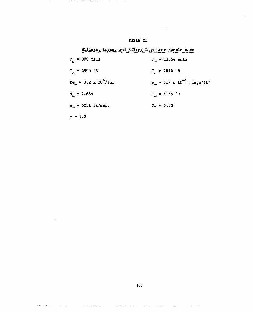
TABLE I1

Elliott. Bartz. and Silver Test Case Nozzle Data

Po = 300 p i a P, - 11.54 psia

To 0 4500 OR T, 9 2614 OR

Re, 0.2 x 10 /in. 6 = 3.7 x slugs/ft 3

M, = 2.685 Tw = 1125 O R

u, - 6231 ft/secr Pr = 0.83

y 1.2

/

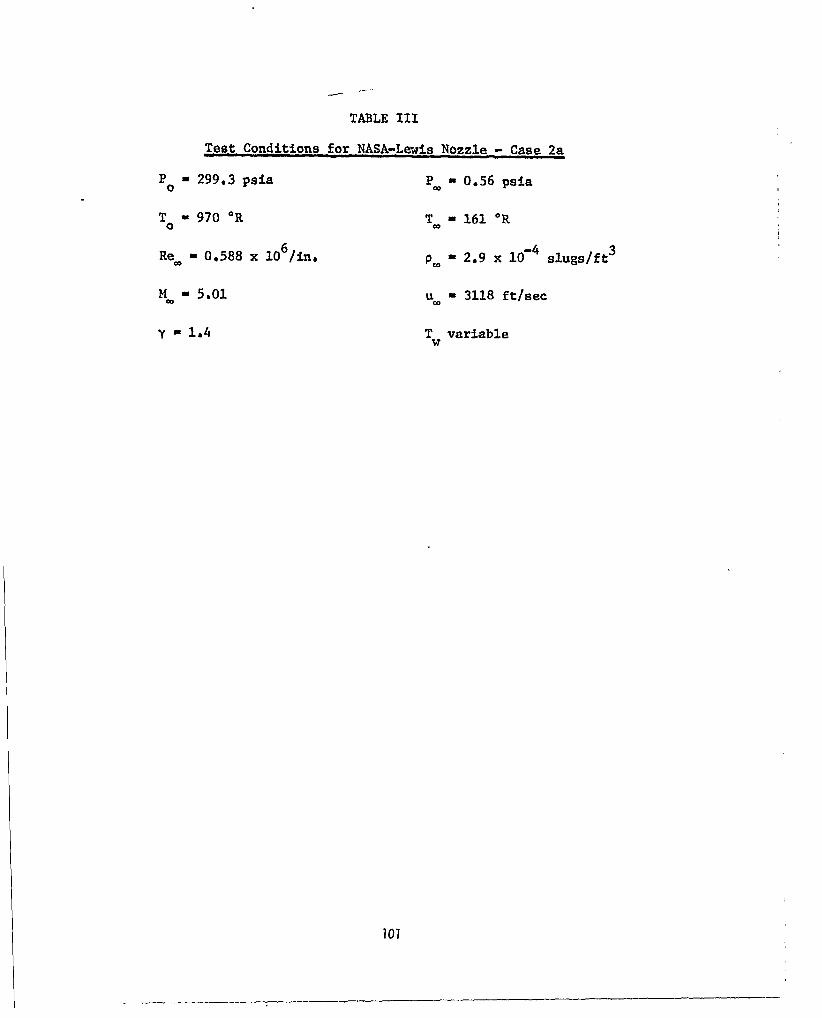
TABLE I11

Test Conditions for NASA-Lewis Nozzle - Case 2a

Po 9 299.3 psia P, - 0.56 psia

To 970 O R T, - 161 O R

Re, = 0.588 x 10 /in, 6 p, - 2.9 x loo4 slugs/ft 3

M, 5.01 u, 3118 ft/sec

y 9 1.4 Tw variable

I

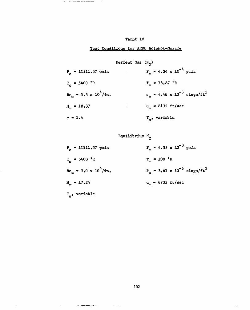
TABLE I V

Test Conditions for AEDC Hotshot-Nozzle

Po = 11511.57 paia

To = 5400 OR

Re, 5.3 x 10 /in. 4

M, 18.37

y 1.4

= 11511.57 ps ia

To = 5400 OR

Re, = 3 .O x 10 /in, 4

M, 17.24

Tw, variable

Perfect Gas (N2)

P, = 4.34 x psia

T, = 78.87 OR

4.46 X 8lUgE/ft 3 PC0

u, = 8132 ftjsec

Tw , variable

Equilibrium N2

P, = 4.33 x 10’~ psia

T, = 108 O R

P, 3.41 X low6 BlUgE/ft 3

u, = 8732 ft/sec

102

TABLE V

Test Conditions for Hironimus' Flat Plate Experiments

Po 8498 psia

To - 4913 O R

Re, 4.46 x 10 /in 5

M, = 7.391

Tn - 533 O R

Po = 14670 psia

To = 3691 O R

Re, = 1.33 x 10 /in 6

M, 9 7.58

Tn = 355 O R

Case 1

P, = 1.53 p s i a

T, - 546 O R

- 2.49 x slugs/ft 3 p,

uW = 8157 ft/sec

Case 2

P, - 2.46 p s i a

T, = 339 O R

p, = 6.1 x lom4 slugs/ft 3

u, - 6843 ftisec

103

i

TABLE VI

Flight Conditions for AGARD Test Case A

PA = 6.035 atms P, - 1.0997 x atms

TA - 6996 "K T, - 226.98 OR

Re, = 2157943/ft ALT - 100,000 f t

M, 20.178 r = 1 i n n

u, 20,000 f t / s e c Tw - 1400 O K

1 04

TABLE VI1

Flight Conditions for Sphere-Cone Sample Case

PA/P, = 513.994 P, 4,429 x loo2 atms

TA/T, - 33.065

P;/P, 11.783

T, = 217.9 O K

P, = 5.555 x lo1* AMAGAT

M, 19.564 A l t - 70,000 f t

Re, = 8.898 x 106/ft Tw - 1000 "R

u, - 19,000 f t / s ec Y: - 1.1655

TABLE VI11

Test Conditions for Flat Pla te F lows wtth Mass Injection

Run x, ran Rexx lom6 pw “w Tw’Te Me TeOK p 11 :

- x 10 4

NO e e

5

6

7

8

9

10

11

12

13

14

15

16

17

18

19

2,925

3,446

4 160

4.261

3.249

3,950

4 264

3,185

3 619

. -

3.945

4 a 298

3,057

3.163

3 679

4.260

6.38

6.49

6 a 6 0

6.48

6.39

6 e.42

6.37

6.28

6.20

6.22

6.22

6.52

6.32

6.44

6.45

4 .x02

4 132

4 263

4 167

4 .lo2

3.991

3 808

3 864

3 640

3.759

3.662

4.418

4 .171

4.346

4 297

60 04

58e1

5603

5803

59 e5

59 0 1

60 ,O

61.9

62.4

62.5

62.5

57.6

61.0

59 00

58.6

106

9.23

9 b o 7

8.85

9.21

16.86

16 24

17.81

24.91

24.52

24.90

25.80

0.0

0.0

0.0

0.0

TABLE Ut

Comparison of Numerical Predictions and Experimental Data for Flat Plate Flaws with Mass Injection

exp b

19

calc

exp b 3 I-.

8

calc . exp .

11

calc

exp b

15

calc

530 2

530.2

530.2

8034 7

8036.6

8042 2

12.54

0.0

11.95

8.39

9 e21

4 902

5.17

17 a81

2.59

3.40

$30.2 8106.4 25.8

0.376

0,409.

0.658

0.665

0.934

0.996

1.25

10 b o

10 b 1

14.1

15.4

18 .O

21.8

22.7

3023 15.11

3284 14.06

5288 11.94

5341 14.40

7511 11.46

8009 14.23

10166 11 36

1.50 1.54 1.34 19.2 28.5 10820 14.39

Figure 1: Boundary Layer Coordinate System

0.7

0.6

0.5

0.4

8’ in. 0.3

0.2

0. I

0

I I I I I I I I I

0 IO 20 30 40 50 60 70 80 90 100 .X, in.

Figure 2: Displacement Thickness f o r Flat Plates-Coles Data

c

1.0

0.8

- U Ue 0.6

0.4

0.2

0

M a = 3.701 x = 21.48 in. Reco,,=3.54xlO6

EDDY VISCOSITY MODEL ”” VAN DRIEST

REICHARDT -.-.-.

6) COLES CASE 20

0 0.1 02 0.3 0.4 0.5 0.6 y, inches

Figure 3: Velocity Profiles for a Flat-Plate-Coles Data

110

30

25

20

t~+ 15

IO

5

0

Ma= 3.701 X = 21.48in. Rea,x = 3.54 X IO6

VAN DRIEST (1956) / COLES CASE 20

I

FAIRING O f EXPERIMENTAL DATA

EDDY VISCOSITY MODEL ""_ VAN DRIEST -.-.-.-. REiCHARDT

I I I I 1 1 1 1 I I I I I I I I I I I I i l l

IO0 io ' I o' Y+

Figure 4: Velocity Profiles for a Flat Plate-Law of the Wall Variables-Coles Data

111

I os

2.5

I .5

Y 8 -

I .o

0.5

0 1

I 1 I “I I I

EDDY VISCOSITY MODEL

”” VAN DRIEST M, = 3.701 RE ICHARDT x = 21.48

Rea= 3.54 x IOg COLES CASE 20 -

- .- .-.-

O 10 : 20 30 40 50 60 70 C 4 = E

U

Figure 5: Comparison of Eddy Viscosity Profiles for a Flat Plate-Coles Data

I”

I 0-2 - I I I I I l l 1 1 I I I 1 I I l l _ ‘ - COLES EXPERIMENTS

0 3.701 CASE 20 m 4.544 CASE 62 1

- A 2.570 CASE 26 -

- -

Ma -

- - -

4

1

PRESENT RESULTS EDDY VlSCOSlTY MODEL

I

“-” VAN DRIEST REICH ARDT -.-.-.-

I 1 I I I I I I I I I 1 I I I I l l ,

I o6 lo7 108 Re,,x

Figure 6: Skin-Friction Distribution for a Flat Plate-Coles Data

113

r = 2.50

1-42 1 ALL DIMENSIONS in.

L ro = 0.885

”* r ~1.85

Figure 7s Nozzle Geometry-Elliott, Bartz, and Silver Test Case

P,=3OOpsi T,=4500°R, B=6.5

CURVE I'MODEL I CEBECI 8t SMITH 2 VAN DRIEST 3 I DPf 0x1 4 REICHARDT

0 IO 20 30 40 50 60 70 80 €+

Figure 8: Eddy Viscoeity Profiles at Nozzle Throat-Elliott, Bartz, and Silver Test Caae

115

PO = 300 psi , TO = 4500O R

28 I I I I 1 I I I I T H RpAT

4 PRESENT RESULTS

0 I I I I I 1 I I 0 0.1 0.2 0.3 0.4 0.5 0.6 0.7 0.8 0.9 1.0

Z/L

Figure 9r Heat Transfer Distribution Along Nozzle Wall-Elliott, Bartz, and Silver Test Case

Po = 3OOpsi, TO = 4500OR

0.28 I 1 I I 1 1. I I

”- ELL1 OTT, BARTZ ,8r Si LVER PRESENT RESULTS 0.20

-

8, in. 0.16

0.12

0.08

0.04

0

Figure 101 Boundary Layer Thickness Distribution for a Nozzle-Elliott, Barez, and Silver Teet Caee

.

I 0.024

0.020

0.016

\

o.o'2 t \\ PRESENT RESULTS 0.008 1 \ "- ELLIOT, BART2 & StLVER

\

I s", in \ 2b Po = 3OOpsi I

""

-0.004 1 -0.008

0 0.1 0.2 0.3 0.4- 0.5 0.6 0.7 0.8 0.9 1.0 Z/L

i

0.032

0.028

0.024

0.020

8,in 0.016

0.012

0.008

0.004

0

1 I I I I 1 1 I I

= 3OOpsi - To = 4500OR ELLIOTT, BARTZ, & SILVER PRESENT RESULTS

"-

1 K ~ ~ ~ N A L ENTRANCE CONDITIONS I -\ CASE

1.00 0 0 0 0 I - \ c d e A 8 \ I I I

-\ '\ 2a 0.188 0.201 0.022 0.024 1.01 ,

/

- \ \ 2b 0.188 0 0.018 0 0 / /

- \

THROAT / I ' ' \ ', \2a

\ \ I I /'

/

0 0.1 0.2 0.3 0.4 0.5 0.6 0.7 0.8 0.9 1.0 Z/L

Figure 121 Momentum Thickness Distribution for a Nozzle-Elliott, Bartz, and Silver Test Case

r9 in.

I

Figure

,

3 - -

-

-

0 I I I I I I I I I I I I

0 2 4 6 8 10 I2 z, in.

13; Geometry f o r the NASA-Lewie Nozzle

i

P 'PO

I I I

-EXPERIMENTAL --- I- D EXPANSION

Po = 300 PSIA T, = 970"R

I I I I I I I I I I I I I I I I l l I I I 1 1 1 1 1

I 0" ioo IO+' z

Figure 142 Pressure Distribution for the NASA-Lewis Nozzle

900

800

700 0 .. I- P 600

500

Figure 15% Wall Temperature Distribution for the NASA-Lewis Nozzle

.. i

75X I 0-4

60X IO-^

40X I 0-4

2 o x m 4

""

-.-

PRES. METHOD EXPERIMENT Po = 300 PSIA .

AXIAL DISTA.NCE ALONG NOZZLE 9 in= Figure 16, Heat Tranefer Distribution for the NASA-Lmie Nozzle

. . .

6 I I I I I I I. I

THROAT

4 - rx=o.055 in x / r" = IO. 30 -

r - 4

13 L r" If 5 O 7

i

~ X / P

I 1 i I 1 I I I I , 0. i 0 4 8 12 16 20 24 28 32 36 I

I Figure 17: Geometry for the AEDC Hotshot-Nozzle

t

!

7000 I I I I I I 1 A I I "

6000

5000

4000 , Pw

3000

2000

I O 0 0

30 ms n

t \\ ms- TIME IN MILLISECONDS

0 IO 20 30 40 50 60 70 80 96 2000

z/r Figure 18t Wall Enthalpy Distribution for the AEDC Hotshot-Nozzle

. . . . . . .

3

2

I

0 n

a" Y a. -I \

-3

-4

I I I

a Pw MEASUREMENT 0 Pw DEDUCED FROM P i MEASUREMENTS

Po = I 1,500 psi

z/r Figure 19r Preseure Distribution for the AEDC Hotshot-Nozzle

0 100 200 300 E'

. . . . . .

IO 4

V W cn

Figure 213 Heat Tzansfer Distribution for the AEDC Hotshot-Nozzle

0.6 I I 1 I I 1 I I I

0.5 -

0.4 -

ax rR - 0.3-

0.2 -

0.1 -

""

VAN DRIEST REICHARDT

PO = 11,500 psi

} EDDY-VISCOSITY LAW

T o = 5,400 O R

y = 1.4

I I I I I

Figure 221 Displacement; Thickness Distribution for the AEDC Hotshot-Nozzle

2400

2000

v) 2 0

Q rar w t-

LL 0

1600

- 1200

0

a

I- 400

800

!3

0

I I I I 1 I I EDDY VISCOSITY LAW I .

I RlCHAWDT - 1

"" VAN DRIEST

0 400 800 1200 1600 Z/P *

Figure 23: Number of Iteratione Required to Obtain a Converged Solution

IO

a

6 * 0 - % Q)

33 4

2

0 0

I I I I I

1 =-\

0 EXPERl M ENT

- PRESENT METHOD "e FULLY TURBULENT

FULLY LAMINAR 0 Mao= 6.928

- TO = 6082OR 0 Tw= 533OR 1

I I I I I 1 I 2 4

Re, X IOw6 6 8 IO

Figure 24r Skin Friction Disttibution for a Flat Plate-Hironimue' Data Case I

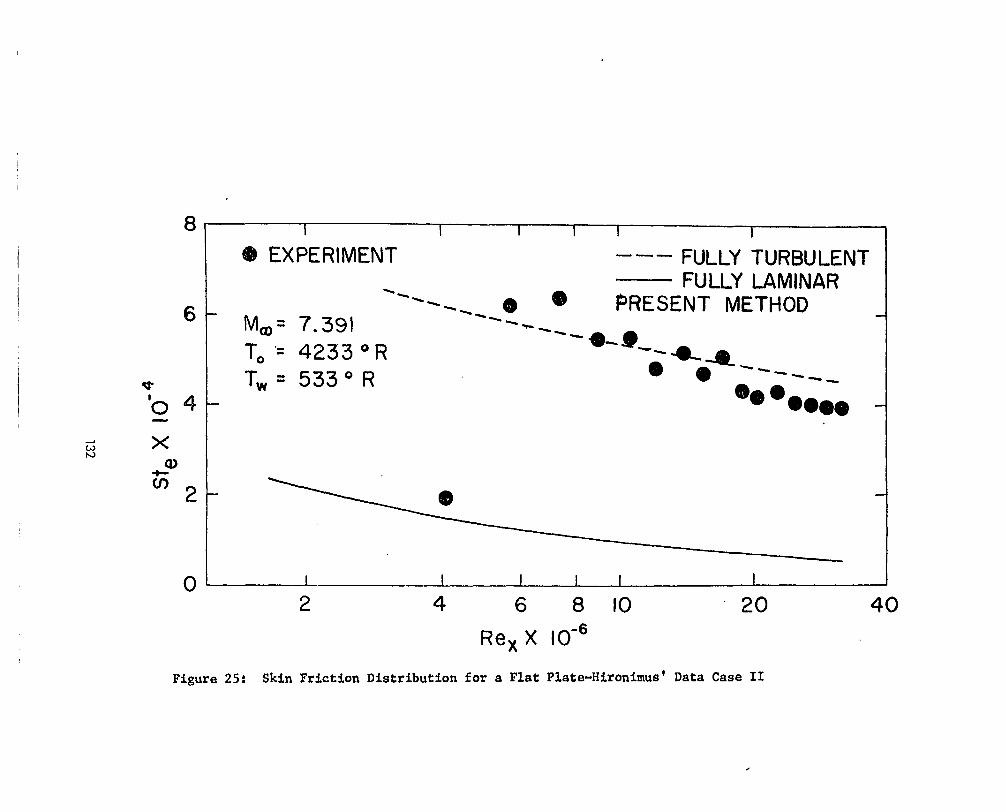
8

6

* '0 4 -

0

EXPERIMENT "- FULLY TURBULENT FULLY LAMINAR

" " -" @ e PRESENT METHOD Ma= 7.391 To '= 4233 O R

T, = 533 O R

" " "'*-.6, ;**a- -" * "

- %@..a@

1 I I I I I 1 2 4 6 8 IO 20 40

Re, X

Figure 25: Skin Friction Distribution for a Flat Plate-Hironimus' Data Case 11

14 12 IO 8 6 4 2

-4 -6 -8 -10 -12 -14

I I I I I I 1 I I I

0 5 10 15 20 25 30 35 40 45 50 Z J r ,

Figure 26: Geometry for a 10' Half-Angle Hyperboloid-AGARD Case A

PRESSURE DISTRIBUTION - MODIFIED NEWTONIAN

THEORY ,

I oo

IO"

Bigute' 27t Pressure Distrlbution for a 10' Half-Angle Hyperboloid-AGARD Case A

I

0.09

0.0 8

0.07

0.06

0.05 - S* 'n

0.04

0.03

0.02

0.0 1

0

AGARD CASE A 100,000ft/20,00Oft/sec. -

Tw= 1400K

PRESENT METHOb

Po = 6.0352 ATMS To = 6996 O R Re,= 2157943 / FT M a = 20.17-8

0 10 20 30 40 50 S/r,

Figure 288 Displacement Thickness Distribution €or a 10' Half-Angle Hyperboloid-AGARD Case A

I o'2

cfa

I o - ~

-7 IXGARD CASE A

100,000ft/20,000ft/sec.

PRESENT METHOD

BLOTTNER, NEQ, MCW or ECW

SCHONAUER EQUIL

pd = 6.0352 ATMS To = 6996"R RE+,, = 2157943/FT M, = 20. I78

10'' I I I I I I I l l I I I I I I l l 1 I I I 1

IO" I 10 50 S/r,

Figure 29: Skin Friction Distribution for a 10' Half-Angle Hyperboloid-AGARD Case A

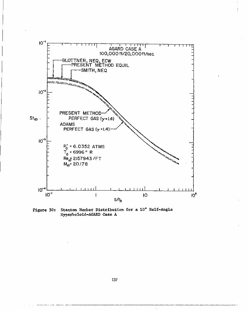
IO" - I I I 1 1 1 1 1 I I I I 1 1 1 1 1 - I - I I 1 1 1 1 1 ' - AGARD CASE A - - - 100,000 ft/20,000ft/sec. -

I 0-2

PRESENT METHOD

PERFECT GAS (7 =1.4)

P i = 6.0352 ATMS

I o - ~ I I I I 1 1 1 1 I I I I I I l l I I I 1 I I l l

IO" I IO IOe sir,

Figure 30: Stanton Number Distribution for a 10' Half-Angle Hyperboloid-AGARD Case A

137

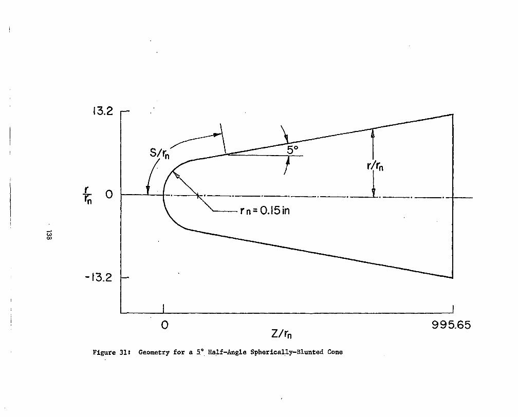
13.2

T ' 0

-13.2

Figure

0 Z/f"

311 Geometry for a 5'. Half-Angle Spherically-Blunted Cone

9 9 5.65

P

IO"

1 0 3

334.645 19.564

DE = 70,000FT

Figure 32: Pressure Distribution for a 5' Half-Angle Spherically-Blunted Cone

.. . . .

I o-~ I I I I 1 1 1 1 1 I I I 1 I I111 I I I I I l l I .Q 10 I o2 I os

s /r,, Figure 348 Displacement Thickness Distribution for Turbulent Flow

Over a 5' Half-Angle Spherically-Blunted Cone

141

I P,' = 334.645 PSlA

Re, = 8.898~ IOe/FT ALTlTU DE = 70,000 FT

Ma = 19.564.

- EQUIUBRIUM

IO0 IO' IO2 103 s/rn

Figure 358 Skin Friction Distribution for a So Half-Angle Spherically-Blunted Cone

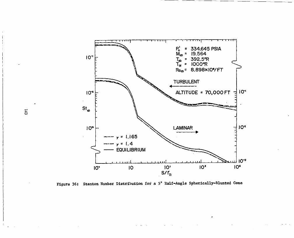
I I I I 1 1 1 1 I I I I I I l l I I I I 1 1 1 1 '

P,' = 334.645 PSlA

Tco = 392..5"R Ma = 19.564

- - Tvr = t0OQ"R

F

I o*

IO' IO' I os s/ rn

Figure 368 Stanton Number Distribution for a 5' Half-Angle Spherically-Blunted Cone

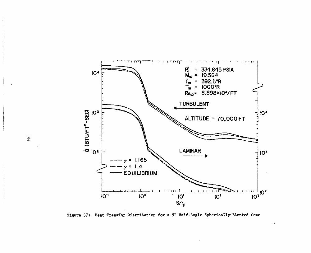
E '

334.645 PSlA 19.56.4 392.5OR IOOOOR 8.898xIO"r 1 -

TURBULENT - 1 104

ALTITUDE = 70,000 FT -

-*\- -.-a"-. -".:

y = 1.165 y = 1.4 EQUlLlSRlUM

I I I r 1 1 1

IO0 . IO' IOP S/r,

1 , IO3

10 = IO3

F5gure 371 Heat Transfer Distribution for a 5" Half-Angle Spherically-Blunted Cone

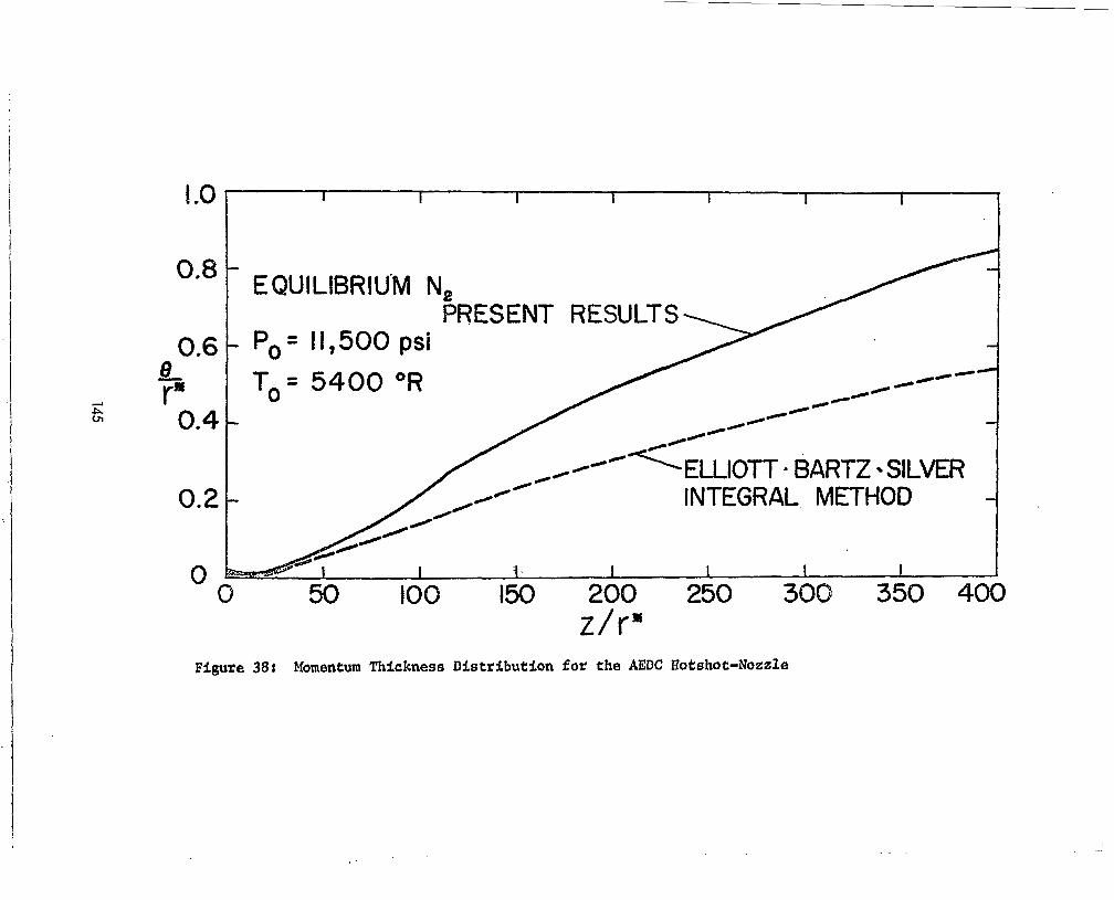
i c .O

8.8

0.6

p. cn 0.4

0.2

I I I I I 1 I

EQUILIBRIU'M N,

Po= 11,500 psi

To= 5400 O R

PRESENT RESULTS

/ "- )C"

c)

-'flKELLIOJ-r = BARTZ SILVER fNTEGRAL, METHOD -

I I I I

358

Figure 388 Momentum Thickness Distribution for the AEDC Hotshot-Nozzle

20

16

8 y“ 12 and

4

I 1 I 1 I I I I “- ELLIOTT-BARTZ- SILVER

PRESENT’ RESULTS EQUILIBRIUM N, Po = I 1,500psi T, = 5400 O R

IO0 200 300 400

Figure 39: Boundary Layer and Displacement Thickness Distribution for the AEDC Hotshot-Nozzle

to4

EQUILIBRIUM N, Po = 11,500 PSI To = 5,400°R

I

Figure

I IO 10, Z I P

to3

40; Hear Transfer Distribution for the AEDC Hotshot-Nozzle

!

147

2. I I I I I

ELLIOTT-BARTZ-SILVER - ENKENHUS-MAHER .POWER LAW VELOCITY

CROCCO ENTHALPY' AND ENTHALPY PROFILES

'EQUILIBRIUM N2 Z/rm= 984 PO= 1.1,500 psi

To"5400°R PRESENT METHOD

P ' P E Figure 41: Density Profiles for the AEDC Hotshot-Nozzle

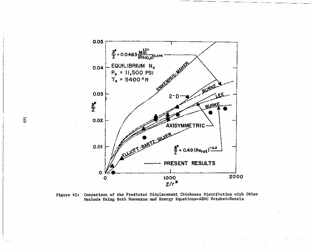
0.05 1 I 1

0.04

0.03

0.02

0.01

\

PRESENT RESULTS

0 I 0 1000 2000

z/r ' Figure 422 Comparison of the Predicted Displacement Thickness Distribution with Other

Methods Using Both Momentum and Energy Equations-AEDC Hotshot-Nozzle

. . - EQUILIBRIUM N,

(a) "- EDENFIELD'S RESULTS To = 5400 OR I00 I I I I I I I I . I I

PRESENT RESULTS Po = I1,5OOpsi

G 0

A Pw MEASUREMENT MOMENTUM EQUATION ONLY P ' MEASUREMENT 0 CROCCO ENTHALPY DISTRIBUTION

ELLIOTT BARTZ SILVER INTEGRAL ME THO0

0 400 800 1200 I600 2000 z/r#

Figure 43; Comparison of the Predicted Displacement Thickness Distribution with Other Methods Which Use the Momentum Equation Only-AEDC Hotshot-Nozzle

4 1 I I 1 I I I I I , I I I I I I I ' I I I I I I 1 1 7

I "THROAT 3 -

2 -

A

$a I - n.

0-

Y

0

3 0 -

-1 -

- 2 -

' \ Po = 58522 PSIA f0= 1 0 ~ 0 ~

-.- EQUILIBRIUM AIR EQUILIBRIUM N2 -

-..- PERFECT GAS Nz

M a = 10.62 M a = 13.69 M a = 21.64

-3 I I I I I I I l l I I I I I 1 1 1

Io-I I oo Z, in IO' IO2

Figure 441 Pressure Distribution for the AEDC Nozzle Configuration=Po - 58,522 PSIA; To = 10,OOO°K

Figure 45 :

152

IOP 1 I I I I l l l l 1 I I I l l l l l I I I I 1 1 1

t"

Figure 46: Stanton Number Distribution for the AEDC Hotshot-Nozzle Configuration-Po - 58,522 PSIA; To - 10,OOOOR

153

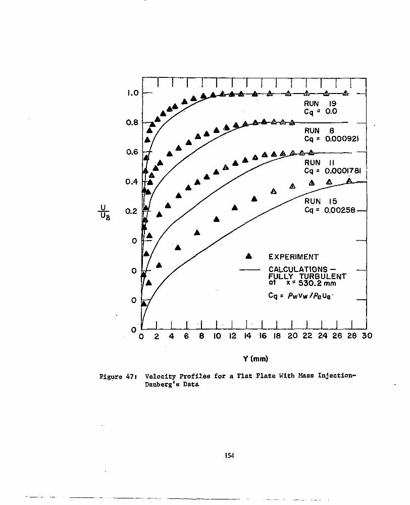
I I I I 1 I I I I I I I I I I

7"" RUN 8 Cq = 0.000921

0.6

- CALCULATIONS - FULLY TURBULENT at X = 530.2 mrn

I " I - I I - I I I 1 I I I J 0 2 4 6 8 IO I2 14 16 18 20 22 24 26 28 30

Figure 47: Velocity Profiles for a Flat Plate With Mass Injection- Danberg'a Data

154

,.e - e :H,-H,J --- LAMINAR - FULLY TURBULENT

-

I "

lo5 I o6 R e X

I 0'

I

I

t ERG EXPERIMENTAL DATA. NOMINAL VALUES NUMBERS I 16- 19 I 5-8 I 9-1 I I 12-15

~~ ~~ - -

SYMBOL BI e A 6- Me 6.4 6.5 6.4 , 6.24

4.31 4.17 3.94 3.73 w V w / P e U e X IO4 0.0 9.09 17.0 25.0 -

RUN 19

RUN 8

RUN 19 RUN I 1

RUN 15

. _

I os

Figure 49: Skin Friction Distribution for a Flat Plate With Mass Injection-Danberg's Data

NASA CONTRA CTOR NASA - ntrs.nasa.gov. Report No. 2. Government Accession No. 3. ReLnp,mmro wra10g...

Documents

Transcript of NASA CONTRA CTOR NASA - ntrs.nasa.gov. Report No. 2. Government Accession No. 3. ReLnp,mmro wra10g...