Naoyuki Yoshino and Victor Pontines - IMF · Naoyuki Yoshino and Victor Pontines Dean Research...
32
Impact Evaluation of Infrastructure: Case Studies of Japan and the Philippines Naoyuki Yoshino and Victor Pontines Dean Research Fellow Asian Development Bank Institute [email protected] / [email protected] IMF-Japan High-Level Tax Conference Tokyo, Japan, 7 April 2015 1
Transcript of Naoyuki Yoshino and Victor Pontines - IMF · Naoyuki Yoshino and Victor Pontines Dean Research...

Impact Evaluation of Infrastructure: Case Studies of Japan and the
Philippines
Naoyuki Yoshino and Victor Pontines Dean Research Fellow Asian Development Bank Institute
[email protected] / [email protected]
IMF-Japan High-Level Tax Conference
Tokyo, Japan, 7 April 2015
1

Outline
1, Micro data-based Evaluation of the effect of Infrastructure – Philippine case 2, Tax revenues and Non-tax Revenues 3, Business Tax, Property Tax 4, Affected region vs non-affected region 5, Macroeconomic effect of infrastructure 6, Community based infrastructure Hometown Investment Trust Funds
2

Micro Case Study - Philippine micro data Objectives:
1, Evaluation of the ‘highway effect’ on tax and non-tax revenues using as case study the Southern Tagalog Arterial Road (STAR) in Batangas Province, Philippines
2, Evaluation is carried out using a quasi-experimental approach via a difference-in-difference (DiD) analysis
3

Affected or treatment group (D = 1)
Affected group: Lipa City, Ibaan and Batangas City
4

Unaffected or Control groups (D = 0) Control group (1): San Jose San Pascual Padre Garcia Rosario Taysan
5
Control group (2): Cuenca Alitagtag Bauan Lobo San Juan
Control group (3): Agoncillo Lemery San Nicolas Taal San Luis Mabini
Control group (4): Nasugbu Lian Tuy Balayan Calaca Calatagan

Method: Difference-in-Difference (DiD) Analysis
Pre- Post
where: D = 1 (Affected or treatment group) T = Affected period D = 0 (Unaffected or control group)
= Highway Effect
6
Assumption: Equal trends between Affected and Non-affected groups

Property tax data
7

Business tax data
8

Tax variables and Non-tax variables • We employ data on property tax
revenues, business tax revenues, regulatory fees and user charges of the cities and municipalities comprising Batangas Province, Philippines.
• The tax and non-tax revenues data were obtained from the Philippine Bureau of Local Government Finance (BLGF)
9

10
Difference-in-Difference Regression: Control Group 1 (1)
Property tax
(2) Property
tax
(3) Business
tax
(4) Business
tax
(5) Regulatory
fees
(6) Regulatory
fees
(7) User
charge
(8) User
charge Impact D 1.370
(1.473) 1.466
(1.478) 0.819
(0.869) 0.776
(0.885) 0.932
(0.763) 0.929
(0.779) 0.513
(1.012) 0.612
(1.125) Impact D ×
Periodt-2 0.210** (0.099)
0.095 (0.100)
1.570*** (0.502)
1.616** (0.626)
0.186 (0.121)
0.162 (0.118)
0.651*** (0.132)
0.453*** (0.105)
Impact D × Periodt-1
0.210** (0.096)
0.254** (0.104)
1.689*** (0.517)
1.978*** (0.585)
0.507** (0.225)
0.610*** (0.191)
0.502*** (0.151)
0.330 (0.277)
Impact D × Periodt0
0.342*** (0.125)
0.293** (0.126)
1.849*** (0.519)
1.995*** (0.616)
0.609** (0.292)
0.637** (0.253)
0.740*** (0.175)
0.553 (0.292)
Impact D × Periodt+1
0.373*** (0.128)
0.060 (0.161)
1.799*** (0.536)
1.541** (0.803)
0.774* (0.475)
0.591 (0.458)
0.836*** (0.289)
0.604 (0.470)
Impact D × Periodt+2
0.471** (0.203)
0.183 (0.210)
1.739*** (0.589)
1.520* (0.831)
0.949** (0.430)
0.786* (0.412)
0.803*** (0.267)
0.576 (0.442)
Impact D × Periodt+3
0.376*** (0.123)
0.136 (0.144)
1.968*** (0.479)
1.821** (0.692)
1.162*** (0.290)
1.037*** (0.282)
1.023*** (0.275)
0.804* (0.424)
Impact D × Periodt+4,
forward
1.247*** (0.344)
0.939*** (0.348)
2.610*** (0.280)
2.360*** (0.556)
1.548*** (0.231)
1.369*** (0.272)
1.321*** (0.456)
1.090* (0.603)
Construction 0.709** (0.278) 1.085
(0.920) 0.567 (0.399) 0.118
(0.580)
Constant 16.18*** (0.504)
10.34*** (2.45)
15.25*** (0.516)
6.290 (8.038)
14.84*** (0.272)
10.19*** (3.13)
14.26*** (0.265)
13.39*** (4.85)
N 98 90 98 90 98 90 97 90 R2 0.24 0.25 0.36 0.37 0.42 0.42 0.20 0.21
Clustered standard errors, corrected for small number of clusters; * Significant at 10%. ** Significant at 5%. *** Significant at 1%.

11
Difference-in-Difference Regression: Control Group 2 (1)
Property tax
(2) Property
tax
(3) Business
tax
(4) Business
tax
(5) Regulatory
fees
(6) Regulatory
fees
(7) User
charge
(8) User
charge Impact D 2.283
(1.479) 2.383
(1.486) 1.221
(0.947) 1.078
(0.889) 1.414
(0.843) 1.508* (0.863)
0.775 (1.207)
1.084 (1.30)
Impact D × Periodt-2
0.210** (0.099)
0.109 (0.095)
1.570*** (0.501)
1.686*** (0.614)
0.186 (0.121)
0.101 (0.111)
0.651*** (0.132)
0.319*** (0.076)
Impact D × Periodt-1
0.210** (0.095)
0.248** (0.102)
1.689*** (0.516)
1.930*** (0.580)
0.507** (0.225)
0.652*** (0.188)
0.502*** (0.151)
0.422 (0.272)
Impact D × Periodt0
0.342*** (0.125)
0.297** (0.126)
1.849*** (0.518)
2.017*** (0.614)
0.609** (0.292)
0.619** (0.252)
0.740*** (0.175)
0.513 (0.291)
Impact D × Periodt+1
0.373*** (0.128)
0.101 (0.129)
1.799*** (0.535)
1.760** (0.722)
0.774* (0.475)
0.404 (0.440)
0.836*** (0.289)
0.191 (0.411)
Impact D × Periodt+2
0.471** (0.203)
0.221 (0.191)
1.739*** (0.589)
1.720** (0.766)
0.949** (0.430)
0.615 (0.396)
0.803*** (0.267)
0.199 (0.390)
Impact D × Periodt+3
0.376*** (0.123)
0.168 (0.125)
1.968*** (0.478)
1.986*** (0.638)
1.162*** (0.289)
0.896*** (0.266)
1.023*** (0.274)
0.493 (0.388)
Impact D × Periodt+4,
forward
1.247*** (0.343)
0.980*** (0.334)
2.610*** (0.279)
2.575*** (0.445)
1.548*** (0.230)
1.185*** (0.246)
1.321*** (0.455)
0.683 (0.572)
Construction 0.608** (0.145) 0.554
(0.409) 1.021*** (0.258) 1.120***
(0.192)
Constant 15.27*** (0.529)
10.25*** (1.380)
14.85*** (0.640)
10.30*** (3.596)
14.36*** (0.450)
5.92*** (1.952)
14.00*** (0.712)
4.78** (1.89)
N 102 94 102 94 100 94 100 94 R2 0.41 0.42 0.44 0.45 0.46 0.47 0.18 0.21
Clustered standard errors, corrected for small number of clusters; * Significant at 10%. ** Significant at 5%. *** Significant at 1%.

12
Difference-in-Difference Regression: Control Group 3 (1)
Property tax
(2) Property
tax
(3) Business
tax
(4) Business
tax
(5) Regulatory
fees
(6) Regulatory
fees
(7) User
charge
(8) User
charge Impact D 2.883**
(1.424) 2.941** (1.425)
1.608* (0.850)
1.528* (0.787)
1.824** (0.765)
1.947** (0.805)
1.517 (1.025)
1.879* (1.148)
Impact D × Periodt-2
0.210** (0.097)
0.118 (0.095)
1.570*** (0.489)
1.634*** (0.591)
0.186 (0.118)
0.058 (0.117)
0.651*** (0.130)
0.290*** (0.082)
Impact D × Periodt-1
0.210** (0.093)
0.238** (0.098)
1.689*** (0.504)
1.966*** (0.571)
0.507** (0.219)
0.681*** (0.185)
0.502*** (0.148)
0.442* (0.266)
Impact D × Periodt0
0.342*** (0.122)
0.30** (0.123)
1.849*** (0.507)
2.0*** (0.596)
0.609** (0.285)
0.606** (0.246)
0.740*** (0.171)
0.504* (0.283)
Impact D × Periodt+1
0.373*** (0.125)
0.131 (0.135)
1.799*** (0.523)
1.597** (0.684)
0.774* (0.463)
0.271 (0.449)
0.836*** (0.282)
0.099 (0.409)
Impact D × Periodt+2
0.471** (0.198)
0.248 (0.195)
1.739*** (0.575)
1.571** (0.728)
0.949** (0.419)
0.495 (0.404)
0.803*** (0.260)
0.115 (0.387)
Impact D × Periodt+3
0.376*** (0.120)
0.190 (0.128)
1.968*** (0.468)
1.864*** (0.607)
1.162*** (0.283)
0.797*** (0.280)
1.023*** (0.268)
0.424 (0.385)
Impact D × Periodt+4,
forward
1.247*** (0.336)
1.009*** (0.331)
2.610*** (0.273)
2.415*** (0.412)
1.548*** (0.225)
1.055*** (0.277)
1.321*** (0.445)
0.593 (0.569)
Construction 0.537** (0.167) 0.949**
(0.387) 1.342*** (0.388) 1.342***
(0.260)
Constant 14.67*** (0.451)
10.27*** (1.359)
14.46*** (0.505)
6.64** (3.378)
13.95*** (0.317)
2.88 (3.416)
13.26*** (0.376)
2.18 (2.30)
N 128 118 128 118 128 118 125 118 R2 0.50 0.50 0.47 0.48 0.54 0.57 0.39 0.42
Clustered standard errors, corrected for small number of clusters; * Significant at 10%. ** Significant at 5%. *** Significant at 1%.

13
Difference-in-Difference Regression: Control Group 4 (1)
Property tax
(2) Property
tax
(3) Business
tax
(4) Business
tax
(5) Regulatory
fees
(6) Regulatory
fees
(7) User
charge
(8) User
charge Impact D 1.252
(1.434) 1.491
(1.326) 0.889
(0.865) 0.896
(0.765) 1.326* (0.727)
1.353** (0.692)
1.351 (0.985)
1.789* (0.992)
Impact D × Periodt-2
0.210** (0.098)
0.061 (0.092)
1.570*** (0.495)
1.593** (0.625)
0.186 (0.120)
0.210 (0.137)
0.651*** (0.130)
0.397*** (0.144)
Impact D × Periodt-1
0.210** (0.094)
0.201*** (0.069)
1.689*** (0.509)
1.775*** (0.607)
0.507** (0.222)
0.610*** (0.191)
0.502*** (0.149)
0.474** (0.194)
Impact D × Periodt0
0.342*** (0.124)
0.052** (0.155)
1.849*** (0.512)
1.808*** (0.651)
0.609** (0.288)
0.554** (0.223)
0.740*** (0.172)
0.260 (0.233)
Impact D × Periodt+1
0.373*** (0.126)
-0.230 (0.203)
1.799*** (0.528)
1.617** (0.777)
0.774* (0.468)
0.543 (0.481)
0.836*** (0.285)
-0.150 (0.401)
Impact D × Periodt+2
0.471** (0.200)
-0.071 (0.171)
1.739*** (0.581)
1.584** (0.807)
0.949** (0.424)
0.752* (0.447)
0.803*** (0.263)
-0.084 (0.383)
Impact D × Periodt+3
0.376*** (0.121)
-0.129 (0.164)
1.968*** (0.472)
1.829*** (0.688)
1.162*** (0.286)
0.985*** (0.240)
1.023*** (0.271)
0.193 (0.343)
Impact D × Periodt+4,
forward
1.247*** (0.339)
0.595 (0.386)
2.610*** (0.276)
2.354*** (0.776)
1.548*** (0.227)
1.258*** (0.107)
1.321*** (0.449)
0.266 (0.425)
Construction 1.327** (0.497) 0.60
(0.619) 0.745*** (0.270) 2.137***
(0.641)
Constant 16.30*** (0.440)
5.359 (3.959)
15.18*** (0.521)
10.24** (4.911)
14.45*** (0.184)
8.308*** (2.239)
13.43*** (0.206)
-4.235 (5.14)
N 114 104 114 104 114 104 111 103 R2 0.21 0.23 0.37 0.36 0.56 0.55 0.36 0.44
Clustered standard errors, corrected for small number of clusters; * Significant at 10%. ** Significant at 5%. *** Significant at 1%.

Affected and Unaffected group - Spillover effect (outside of the province)
AFFECTED group: Lipa City, Ibaan and Batangas City Unaffected: (municipalities belonging to neighboring Quezon province) Candelaria Dolores San Antonio Tiaong
14

15
Difference-in-Difference Regression: Spillover (1)
Property tax
(2) Property
tax
(3) Business
tax
(4) Business
tax
(5) Regulatory
fees
(6) Regulatory
fees
(7) User
charge
(8) User
charge Impact D 1.55535
(1.263) 0.736
(0.874) 1.067
(1.316) 0.438
(1.407) 1.372
(1.123) 0.924
(1.046) 0.990
(1.095) 0.364
(1.028) Impact D ×
Periodt-2 0.421** (0.150)
-0.083 (0.301)
1.189*** (0.391)
0.991** (0.450)
0.248*** (0.084)
-0.019 (0.248)
0.408*** (0.132)
-0.010 (0.250)
Impact D × Periodt-1
0.447** (0.160)
0.574*** (0.118)
1.264*** (0.415)
1.502*** (0.542)
0.449** (0.142)
0.515*** (0.169)
0.317** (0.164)
0.434** (0.167)
Impact D × Periodt0
0.497*** (0.128)
0.570** (0.223)
1.440*** (0.417)
1.641*** (0.482)
0.604** (0.183)
0.642*** (0.181)
0.350 (0.271)
0.422 (0.158)
Impact D × Periodt+1
1.294** (0.674)
0.387 (0.728)
2.256** (0.957)
1.779** (0.470)
1.318** (0.649)
0.838* (0.448)
0.959 (0.714)
0.197 (0.560)
Impact D × Periodt+2
1.163* (0.645)
0.336 (0.594)
2.226** (0.971)
1.804** (0.531)
1.482** (0.634)
1.044** (0.413)
0.941 (0.704)
0.247 (0.531)
Impact D × Periodt+3
1.702* (0.980)
0.450 (0.578)
2.785** (1.081)
2.070*** (0.544)
1.901*** (0.630)
1.238*** (0.369)
1.732*** (0.598)
0.676 (0.515)
Impact D × Periodt+4,
forward
2.573*** (0.900)
1.100 (0.758)
3.428*** (0.928)
2.560*** (0.350)
2.288*** (0.563)
1.509*** (0.452)
2.030*** (0.607)
0.787 (0.745)
Construction 2.283** (1.172) 1.577
(1.196) 1.207 (0.855) 1.942*
(1.028)
Constant 14.69*** (0.408)
-2.499 (8.839)
14.18*** (0.991)
2.230 (9.094)
13.66*** (0.879)
4.597 (6.566)
13.08*** (0.649)
-1.612 (7.84)
N 80 73 79 73 80 73 77 73 R2 0.29 0.41 0.37 0.44 0.43 0.50 0.26 0.39
Clustered standard errors, corrected for small number of clusters; * Significant at 10%. ** Significant at 5%. *** Significant at 1%.

Alternative Difference-in-Difference – Distance of municipality from STAR Tollway
• The adjacency of a municipality to the municipality/city in which the STAR Tollway directly pass through was used as the criterion for a municipality to be included in the control group
• We take a different strategy this time by using the estimated distance of a municipality/city from the STAR Tollway
• The difference-in-difference regression is now expressed as:
16 Inclusion of leads and lags as before
17
Difference-in-Difference Regression: Distance from the STAR Tollway (1)
Property tax
(2) Property
tax
(3) Business
tax
(4) Business
tax
(5) Regulatory
fees
(6) Regulatory
fees
(7) User
charge
(8) User
charge
Distance -0.691*** (0.227)
-0.683*** (0.224)
-0.753*** (0.156)
-0.718*** (0.159)
-0.708*** (0.097)
-0.752*** (0.101)
-0.583*** (0.120)
-0.546*** (0.124)
Distance × Periodt-2
0.073*** (0.010)
0.064*** (0.009)
0.166*** (0.010)
0.117*** (0.011)
0.034* (0.018)
0.047** (0.019)
0.107*** (0.016)
0.033** (0.016)
Distance × Periodt-1
0.056*** (0.019)
0.049*** (0.018)
0.205*** (0.013)
0.213*** (0.014)
0.155*** (0.015)
0.173*** (0.013)
0.036 (0.024)
-0.007 (0.025)
Distance × Periodt0
0.103*** (0.011)
0.095*** (0.011)
0.247*** (0.012)
0.222*** (0.012)
0.196*** (0.018)
0.211*** (0.019)
0.120*** (0.029)
0.059** (0.028)
Distance × Periodt+1
0.100*** (0.023)
0.088*** (0.024)
0.230*** (0.015)
0.111*** (0.014)
0.234*** (0.027)
0.241*** (0.025)
0.131*** (0.024)
0.018 (0.027)
Distance × Periodt+2
0.140*** (0.012)
0.130*** (0.015)
0.238*** (0.014)
0.128*** (0.018)
0.292*** (0.022)
0.300*** (0.023)
0.149*** (0.030)
0.042 (0.031)
Distance × Periodt+3
0.111*** (0.020)
0.101*** (0.018)
2.261*** (0.019)
0.168*** (0.023)
0.285*** (0.025)
0.294*** (0.024)
0.181*** (0.023)
0.083*** (0.026)
Distance × Periodt+4,
forward
0.232*** (0.020)
0.220*** (0.023)
0.322*** (0.021)
0.202*** (0.025)
0.370*** (0.016)
0.377*** (0.016)
0.197*** (0.021)
0.084*** (0.027)
Construction 0.030 (0.101) 0.902***
(0.059) 0.077 (0.075) 0.496***
(0.135)
Constant 19.98*** (0.768)
19.74*** (1.108)
19.66*** (0.532)
12.262*** (0.736)
17.946*** (0.334)
17.427*** (0.752)
16.90*** (0.429)
12.930*** (1.255)
N 960 886 960 886 960 886 960 886 R2 0.03 0.03 0.07 0.07 0.12 0.13 0.05 0.04
Clustered standard errors, corrected for small number of clusters; * Significant at 10%. ** Significant at 5%. *** Significant at 1%.

Marginal Productivity of Public Capital (Regional Disparity in Japan)
0
0.1
0.2
0.3
0.4
0.5
0.6
0.7
0.8
Hokkaido Tohoku NorthernKanto
SouthernKanto
Hokuriku Tokai Kinki Chugoku Shikoku NorthernKyushu
SouthernKyushu
SecondaryIndustry
TertiaryIndustry
(C) 2014 Yoshino & Nakahigashi 18

Map of Japan from the North to the South
19
Hokkaido
Tohoku Hokuriku
North Kanto
South Kanto Tokai Shikoku South
Kyushu
North Kyushu
Chugoku Kinki
Okinawa (not included)

Macroeconomic Effect of Public Capital
(C) 2014 Yoshino & Nakahigashi 20
Simultaneous regression of Translog Production Function and Labor Share Function
),,( tttt KgLKpfY =

Marginal Productivity of Public Capital Macroeconomic Effects (in Japan)
(C) 2014 Yoshino & Nakahigashi 21

Effectiveness of Public Capital Stock - “Private capital/Public capital ratio” to “Marginal productivity of Public capital” -
0
0.1
0.2
0.3
0.4
0 0.2 0.4 0.6 0.8 1 1.2 1.4 1.6Private Capital / Public Capital
Mar
gina
l Pro
duct
ivity
of P
ublic
Cap
ital
Southern KantoTokai
Kinki
Chugoku
Northern Kanto
Hokkaido
Southern Kyushu
Tohoku
Northern KyushuShikoku
Hokuriku
(C) 2014 Yoshino & Nakahigashi 22
Secondary Industry (Industrial Sector)

(C) 2014 Yoshino & Nakahigashi 23
Explanation of Direct and Indirect Effects

Table3 Allocation of Public Infrastructure in Japan: (Pooled data, 47 prefecture) Coeffcient Explanatory
Variables Agriculture Land
Conservation Industrial Infrastructure
Improvement of living standardsy
0α Constant -35.44 (-10.46**)
-34.26 (-11.32**)
-61.58 (-11.84**)
52.32 (8.00**)
1α Yp (Income) 0.01 (7.21**)
0.01 (13.18**)
0.02 (17.99**)
0.036 (25.86**)
2α Sp(AreaSize) 4970 (28.47**)
2090 (13.40**)
3855 (14.39**)
2730 (8.10**)
3α Rp(Political Power)
8280 (16.88**)
7274 (16.60**)
10956 (14.55**)
-7434 (-7.85**)
4α Dummy1 -23.21 (-6.69**)
-34.27 (-11.06**)
-59.81 (-11.23**)
-36.85 (-5.50**)
5α Dummy2 27.43 (9.26**)
-1.65 (-0.62)
65.87 (14.48**)
66.89 (11.70**)
Adj. 2R 0.675 0.486 0.458 0.527 (1) ( ) denotes t-value
(2) ** is significant with 99.0% level, (C) 2014 Yoshino & Nakahigashi 24
Determinants of Regional Allocation of Public Investment in Japan (Political Power plays a role)
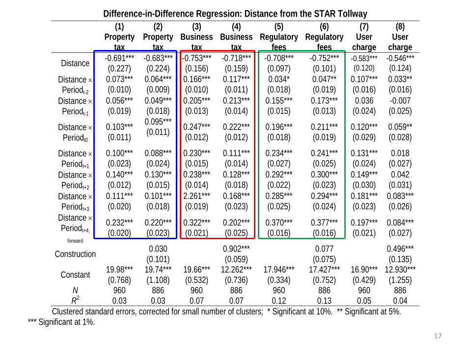
Rate of Return and the Revenue Bond
(C) 2014 Yoshino & Nakahigashi 25
A
B
C D
Rate of return relies on performance of infrastructure
(C) 2014 Yoshino & Nakahigashi 26
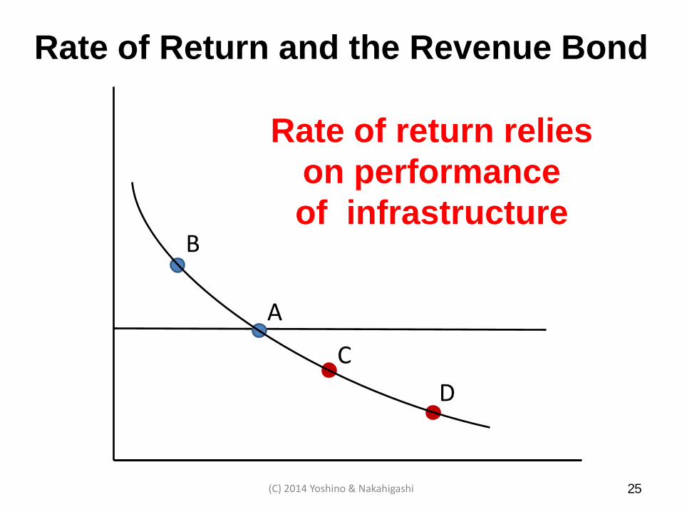
To Create Incentive Mechanism

Public Private Partnership (PPP) (1) Risk sharing between private and public sector (2) Incentive to cut costs and to increase revenue Avoid political intervention (transparency) Bonus payment for employees
who run infrastructure (incentive mechanism) (3) Many projects could be started by PPP Utilize domestic savings Life insurance and Pension funds (long term)
(4) Indirect Effects are important (tourism, manufacturing, agriculture, services)
27

Community Infrastructure
• Wind power Generator Funds • Agricultural Farmer’s Trust Fund • SME Hometown Trust Fund • Local Airport Large Projects Pension Funds, Insurance Funds Infrastructure Bond
28

Hometown Investment Trust
Funds A Stable Way to
Supply Risk Capital (i.e. knowledge
base companies)
Naoyuki YOSHINO Sahoko KAJI (ed.)
29

30

31
Savings/GDP and Investment/GDP in Asia

References: DPWH. Private-Public Partnership Service. Southern Tagalog Arterial Road (STAR) Project. www.dpwh.gov.ph/ppp/projs/star.htm Llanto, Gilberto and Fauziah Zen (2013) “Governmental Fiscal Support for Financing Long-term Infrastructure Projects in ASEAN Countries,” PIDS Discussion Paper No. 2013-08. OECD (2010) Southeast Asian Economic Outlook 2010, OECD Publishing. Yoshino, Naoyuki and Tomohiro Hirano (2010) “Fiscal Stability, the Infrastructure Revenue Bonds and Bank Based Infrastructure Funds for Asia,” GEM Working Paper (Nov. 2010). Yoshino, Naoyuki, Takanobu Nakajima and Masaki Nakahigashi (1999) “Productivity Effect of Public Capital,” in Yoshino, Naoyuki and Takanobu Nakajima (ed.), Economic Effect of Public Investment, Nihon Hyoron-sha, Part I, pp. 11-88. (in Japanese) Yoshino, Naoyuki and Masaki Nakahigashi (2000) “Economic Effects of infrastructure: Japan’s Experience after World War II”, JBIC Review, 3, pp. 3-19. Yoshino, Naoyuki and Masaki Nakahigashi (2004) “Role of Infrastructure in Economic Development,” ICFAJ Journal of Managerial Economics, II(2), pp. 7-26. Yoshino, Naoyuki (2012) “Global Imbalances and the Development of Capital Flows among Asian Countries,” OECD Journal: Financial Market Trends, Volume 2012/1, pp. 81-112. Yoshino, Naoyuki and Sahoko Kaji (ed.) (2013) Home town Investment Trust Funds: A Stable Way to Supply Risk Capital, Springer. Yoshino, Naoyuki and Farhad Taghizadeh-Hesary (2014) “Hometown Investment Trust Funds: An Analysis of Credit Risk,” ADBI Working Paper Series, No.505. Yoshino, Naoyuki and Farhad Taghizadeh-Hesary (2015) “An Analysis of challenges faced by Japan’s Economy and Abenomics” The Japanese Political Economy, Routledge, Taylor and Frances,
32