NANO-SCALE SIMULATION OF GOLD NANOPARTICLE TRACKING …

The Pennsylvania State University

The Graduate School

Biomedical Engineering Department

NANO-SCALE SIMULATION OF

GOLD NANOPARTICLE TRACKING OF KINESIN-1

A Thesis in

Bioengineering

by

Janak Prakashchandra Jethva

2017 Janak Prakashchandra Jethva

Submitted in Partial Fulfillment

of the Requirements

for the Degree of

Master of Science

May 2017

The thesis of Janak Prakashchandra Jethva was reviewed and approved* by the following:

William O. Hancock

Professor, Chair of the Intercollege Graduate Program in Bioengineering

Thesis Advisor

Scott Medina

Assistant Professor of Biomedical Engineering

Peter J. Butler

Associate Dean of Education and Professor of Biomedical Engineering

*Signatures are on file in the Graduate School

iii

ABSTRACT

Kinesins are motor proteins that perform essential cellular functions such as intracellular

transport along microtubules and the organization of mitotic spindle during cell division. The

structure of kinesin-1 consists of two heads attached through flexible neck-linkers to a coiled-coil

stalk that ends in a cargo-binding domain. Kinesin-1 derives energy from ATP hydrolysis and

walks in a hand-over-hand manner with each head taking 16-nm steps along the microtubules. In

published work from the Hancock lab, single molecule experiments were performed to

understand the mechanochemical transitions that underlie kinesin stepping by attaching 30 nm

gold nanoparticle to one of the two heads of kinesin-1 heads through a 14 amino acid Avi-tag.

Using Interferometric Scattering or Dark Field Total Internal Reflection Microscopy, millisecond

temporal resolution and 1 nm spatial precision were achieved in this work. Similar experiments

that showed somewhat different behavior were performed by the Tomishige lab, using a PEG-tag,

which is shorter and less elastic tether than an Avi-tag, and was attached at a different location on

the head.

Interpreting these measurements taken at millisecond timescales requires a more detailed

understanding of the microsecond-scale diffusion of the kinesin head and coupled nanoparticle.

Specifically, it is important to understand how the attached nanoparticle affects the dynamics of

the head and whether the nanoparticle faithfully tracks the head position. To address these

questions, the present study used Brownian Dynamics modelling to simulate the three-

dimensional dynamics of a 30-nm nanoparticle tethered to a kinesin-1 head via either an Avi-tag

or PEG-tag. In the two-head-bound state, a nanoparticle tethered by an Avi-tag tracked the head

more accurately along the axis of the microtubule than a particle tethered through a PEG-tag, but

tracking accuracy perpendicular to the microtubule were identical for the two tethers. In the one-

head-bound state, both heads tracked nanoparticles with similar accuracy, but the PEG-tag

iv

created a larger force in the neck-linker domains than did the Avi-tag. According to these data, an

Avi-tag is a better tag for tracking the head, as it more accurately tracks head position and creates

less perturbation in the natural system than a PEG-tag.

To better study the effects of different experimental parameters on nanoparticle tracking

accuracy, a simpler model consisting of a nanoparticle tethered to a glass surface was used. In

the absence of added experimental noise, particle size and contour length of the tether were found

to have major effects on tracking accuracy, defined as the Root-Mean-Squared (RMS) error

between imaged and true particle position, but the persistence length had only a minor influence.

With simulated experimental noise added, the Avi-tag and PEG-tags gave similar RMS error of

tracking, demonstrating that noise inherent in the imaging process had a larger effect on the

measured particle position than did the mechanical properties of the tether. Kinesins are

implicated in neurodegenerative diseases and are targets for anti-cancer therapeutics, and by

better understanding the inner workings of the motors, it is hope that this work will contribute to

these efforts.

v

TABLE OF CONTENTS

List of Figures .......................................................................................................................... vii

List of Tables ........................................................................................................................... x

Acknowledgements .................................................................................................................. xi

Chapter 1 Introduction ............................................................................................................. 1

1.1 Functions of Kinesins ................................................................................................. 1 1.2 Structure of Kinesin-1 ................................................................................................ 2 1.3 Mechanochemical Cycle of Kinesin-1 ....................................................................... 3 1.4 Single Molecule Experiments with Avi-tagged kinesin-1 ......................................... 5 1.5 Single Molecule Experiments with PEG-tagged kinesin-1 ........................................ 6 1.6 Goals of Simulation ................................................................................................... 8

Chapter 2 Methods ................................................................................................................... 10

2.1 Computational Flowchart ........................................................................................... 11 2.2 Particle Dynamics Simulation .................................................................................... 12

2.2.1 Computational Model for Gold Nanoparticle Tracking Experiment............... 12 2.2.2 Equation of Motion – Langevin Equation ....................................................... 14 2.2.3 Modelling Polypeptides as Entropic Springs using Worm-like Chain

Model................................................................................................................ 15 2.2.4 Volume Exclusion for Particle Collisions ....................................................... 17 2.2.4 Reflective Boundary at Contour Length ......................................................... 17 2.2.5 Implementation in Three Dimensions ............................................................. 18

2.3 Subsampling of Particle Position ............................................................................... 19 2.4 Simulation of the Imaging Process ............................................................................ 19 2.5 Fitting of Particle Tracks ............................................................................................ 21 2.6 Calculation of Statistics.............................................................................................. 22

Chapter 3 Particle Dynamics Simulation of Single Molecule Experiments with Avi-tag

and PEG-tag ..................................................................................................................... 23

3.1 Two Head Bound Case............................................................................................... 23 3.2 One Head Bound Case with Undocked Neck-linker .................................................. 26 3.3 One Head Bound Case with Docked Neck-linker ...................................................... 29 3.4 Comparison of Simulation Data with Experimental Data .......................................... 32

Chapter 4 Accuracy of Tracking by Imaging a Gold-nanoparticle .......................................... 35

4.1 Simplified Model of Tethered Diffusion of Nanoparticle .......................................... 36 4.2 Autocorrelation Time for a Nanoparticle Tethered is on the order of

Microseconds ........................................................................................................... 37 4.3 Effect of Contour Length of Attached Tether on RMS Error of Nanoparticle

Tracking ................................................................................................................... 39

vi

4.4 Effect of Persistence Length of Attached Tether on RMS Error of Nanoparticle

Tracking ................................................................................................................... 40 4.5 Effect of Particle Size on RMS Error of Nanoparticle Tracking ............................... 41 4.6 Effect of Image Noise on Accuracy of Nanoparticle with Avi-tag and PEG-tag ...... 43

Chapter 5 Conclusions and Future Directions ......................................................................... 47

REFERENCES................................................................................................................. 49 Appendix A MATLAB Code for Worm-like Chain Force Calculation .......................... 53 Appendix B MATLAB Code for Particle Dynamics Simulation for Single Molecule

Experiment for One Head Bound Case with Undocked Neck-linker and

Nanoparticle attached with Avi-tag .......................................................................... 54 Appendix C MATLAB Code for Simulation of the Imaging Process ............................ 62 ACADEMIC VITA .......................................................................................................... 64

vii

LIST OF FIGURES

Figure 1-1. Kinesin-1 is a dimer with each monomer having a microtubule-binding head

domain connected via flexible neck-linker to coiled-coil stalk, which ends in a

cargo-binding tail domain. Figure adapted from Asbury et al. [13]................................. 3

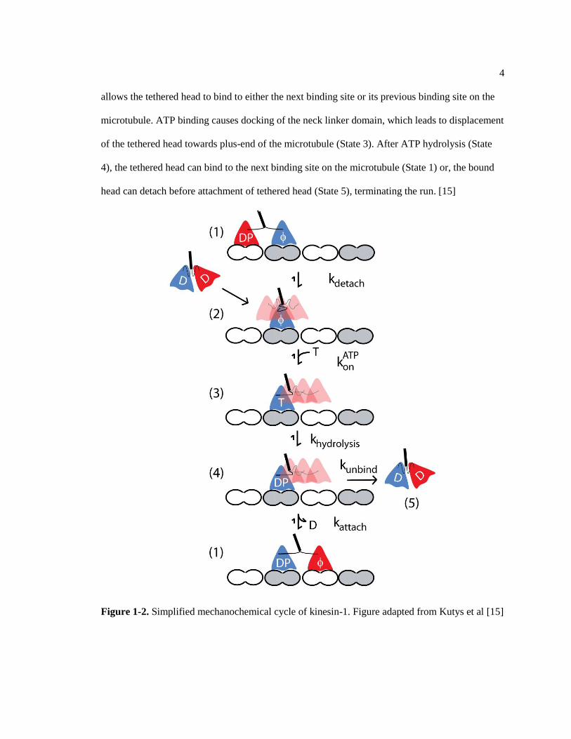
Figure 1-2. Simplified mechanochemical cycle of kinesin-1. Figure adapted from Kutys

et al [15] ........................................................................................................................... 4

Figure 1-3. Experimental setup of a single molecule experiment with 30 nm diameter

gold nanoparticle attached via Avi-tag to N-terminal of kinesin-1 head is shown in

(a). Point spread function of the gold nanoparticle from interferometric scattering

(iSCAT) microscopy is shown in (b). Sample particle tracks from the single

molecule experiments are given in (c), which clearly show 16.4 nm steps. Figure

adapted from Mickolajczyk et al. [16] ............................................................................. 5

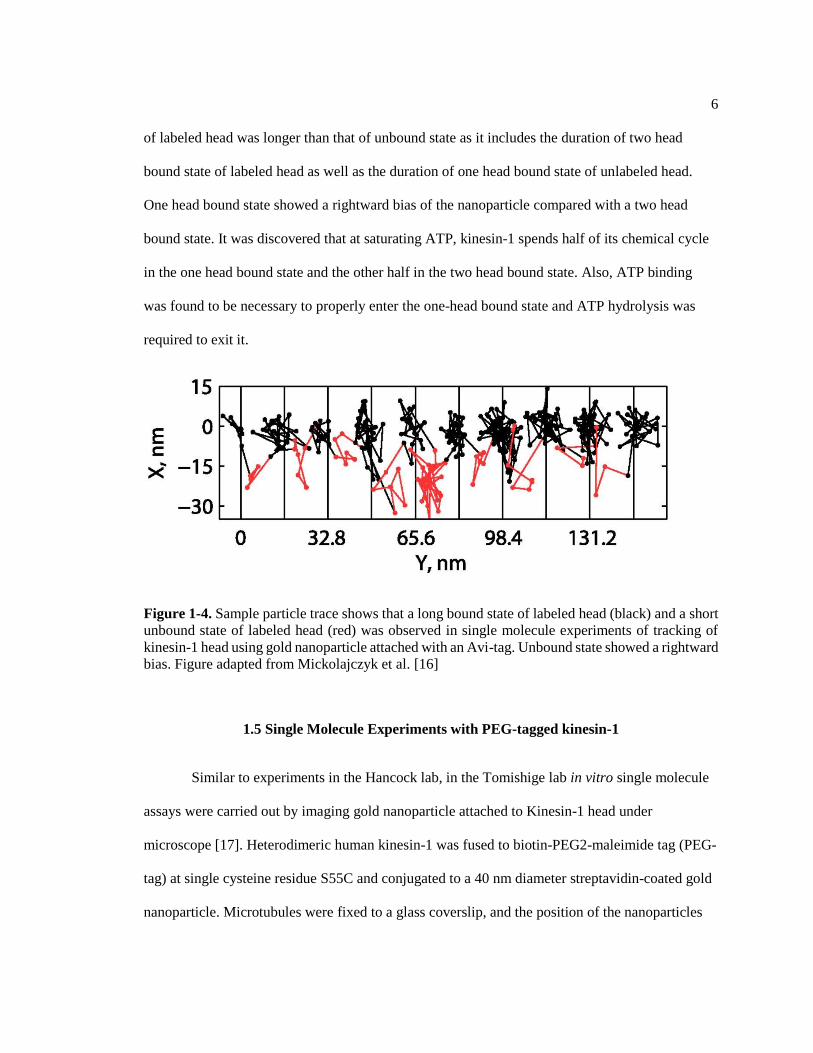
Figure 1-4. Sample particle trace shows that a long bound state of labeled head (black)

and a short unbound state of labeled head (red) was observed in single molecule

experiments of tracking of kinesin-1 head using gold nanoparticle attached with an

Avi-tag. Unbound state showed a rightward bias. Figure adapted from Mickolajczyk

et al. [16] .......................................................................................................................... 6

Figure 2-1. Computational flowchart, which includes particle dynamics simulation to

generate simulated particle positions, which were then subsampled and used to make

simulated movies. These simulated movies were used to fit particle traces to get

measured particle position data, which can then be used to compute error statistics ...... 11

Figure 2-2. Three-dimensional model used for simulation of single molecule

experiments. A 30-nm gold nanoparticle was attached to kinesin-1 at N-terminal of

one of its heads using an Avi-tag. The tethered kinesin-1 was attached to the bound

head through both 14 amino acid neck linker domains, and the particle and tethered

head diffused in three dimensions. The microtubule was modeled as a 25 nm

diameter cylinder. Volume exclusion was maintained in the simulation for the

particle, heads and microtubule, but collisions of the tether with any objects was

ignored. ............................................................................................................................ 13

Figure 2-3. Free body diagram for simple tethered diffusion of a particle in one

dimension. Note that random Brownian force can act in both directions and drag

force always points in the direction opposite to net velocity. .......................................... 14

Figure 2-4. Force-extension profile for kinesin-1 neck-linker. Solid curve is prediction

from worm-like chain model for 15 residue peptide with 0.5 nm persistence length

and 0.38 nm per residue contour length. Figure adapted from Hariharan et al. [27] ....... 16

Figure 2-5. Sample frame from simulation of imaging a fixed nanoparticle with added

shot noise and Gaussian background noise ...................................................................... 21

Figure 3-1. In the two head bound state when the labeled head is bound to the

microtubule, the nanoparticle attached via Avi-tag (shown in a) samples

viii

significantly larger volume than that via PEG-tag (shown in b). The nanoparticle

with Avi-tag tends to stay on the right side of the microtubule. Positions are plotted

at an interval of 1 ns for a total period of 1 ms. The labeled head is shown in red and

the microtubule is shown in green. The nanoparticle position is shown in blue. The

plus-end of microtubule is towards positive x-axis. ......................................................... 24

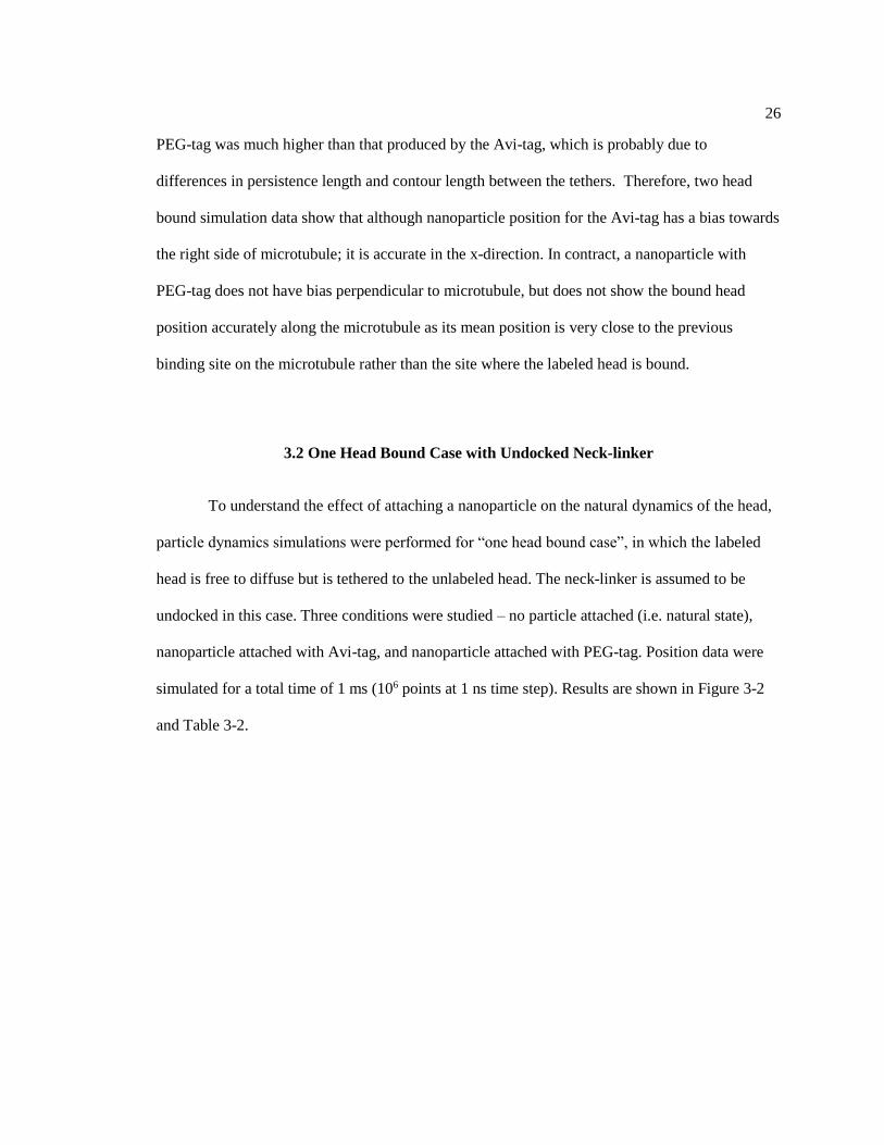
Figure 3-2. In the one head bound state when the labeled head is tethered to the bound

head via undocked neck-linker (a), mean position of the head is skewed towards one

side of microtubule. When the nanoparticle attached using Avi-tag (b) or PEG-tag

(c) to tethered head, the nanoparticle samples larger volume around microtubule

than in the two head bound state, with a bias towards the right side of microtubule.

A nanoparticle attached via PEG-tag samples larger volume than that with Avi-tag.

The microtubule is shown in green and bound head is shown in magenta. Positions

of labeled head (red) and nanoparticle (blue) are plotted at interval of 1 ns for total

period of 1 ms. The plus-end of microtubule is towards positive x-axis. ........................ 27

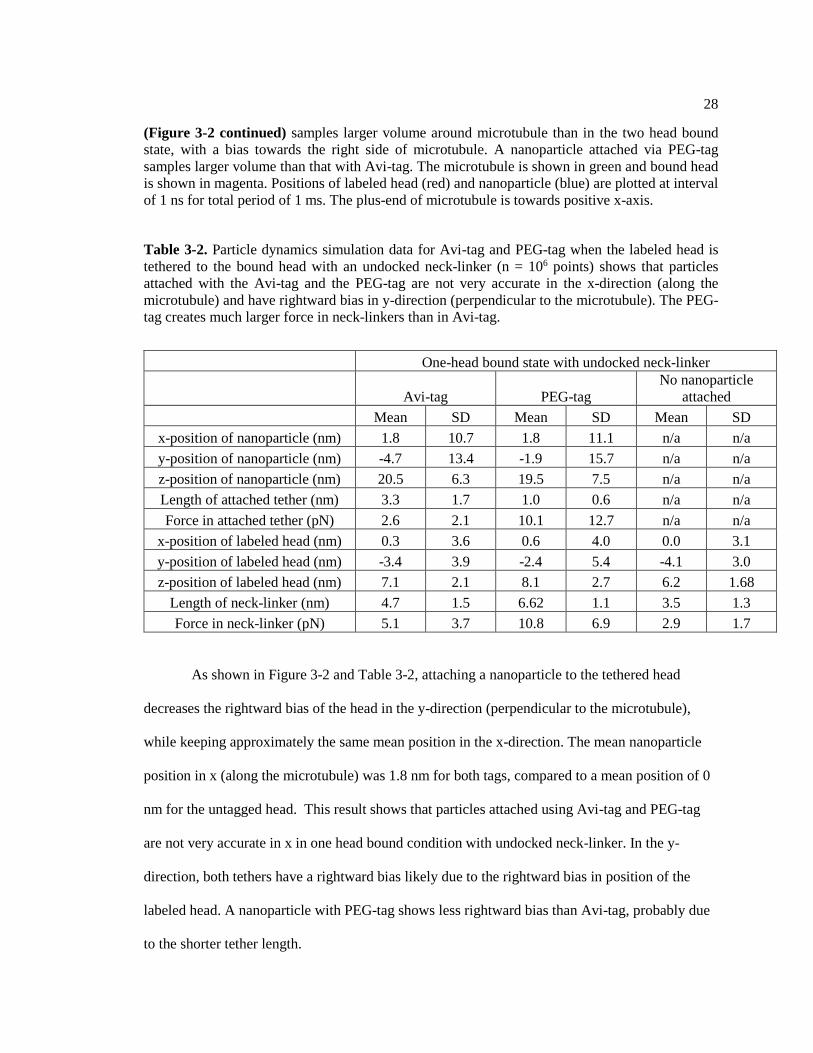
Figure 3-3. In one head bound state when the labeled head is tethered to the bound head

via docked neck-linker (a), the mean position of head is skewed towards right side of

the microtubule due to volume exclusion with the bound head and is shifted towards

the plus-end due to neck-linker docking. When nanoparticle is attached using Avi-

tag (b) or PEG-tag (c) to the tethered head with docked neck-linker, nanoparticle

position shifts in the positive x-direction, while not retaining a rightward bias. Both

tags seem to result in similar nanoparticle position distribution. Microtubule is

shown in green, bound head is shown in magenta and docked part of neck-linker is

shown in black. Positions of labeled head (red) and nanoparticle (blue) at plotted at

interval of 1 ns for total period of 1 ms. Plus-end of microtubule is towards positive

x-axis. ............................................................................................................................... 30

Figure 4-1. Simplified tethered diffusion model of a 30 nm diameter nanoparticle

attached via Avi-tag to a fixed tether attachment point on a glass surface. ..................... 36

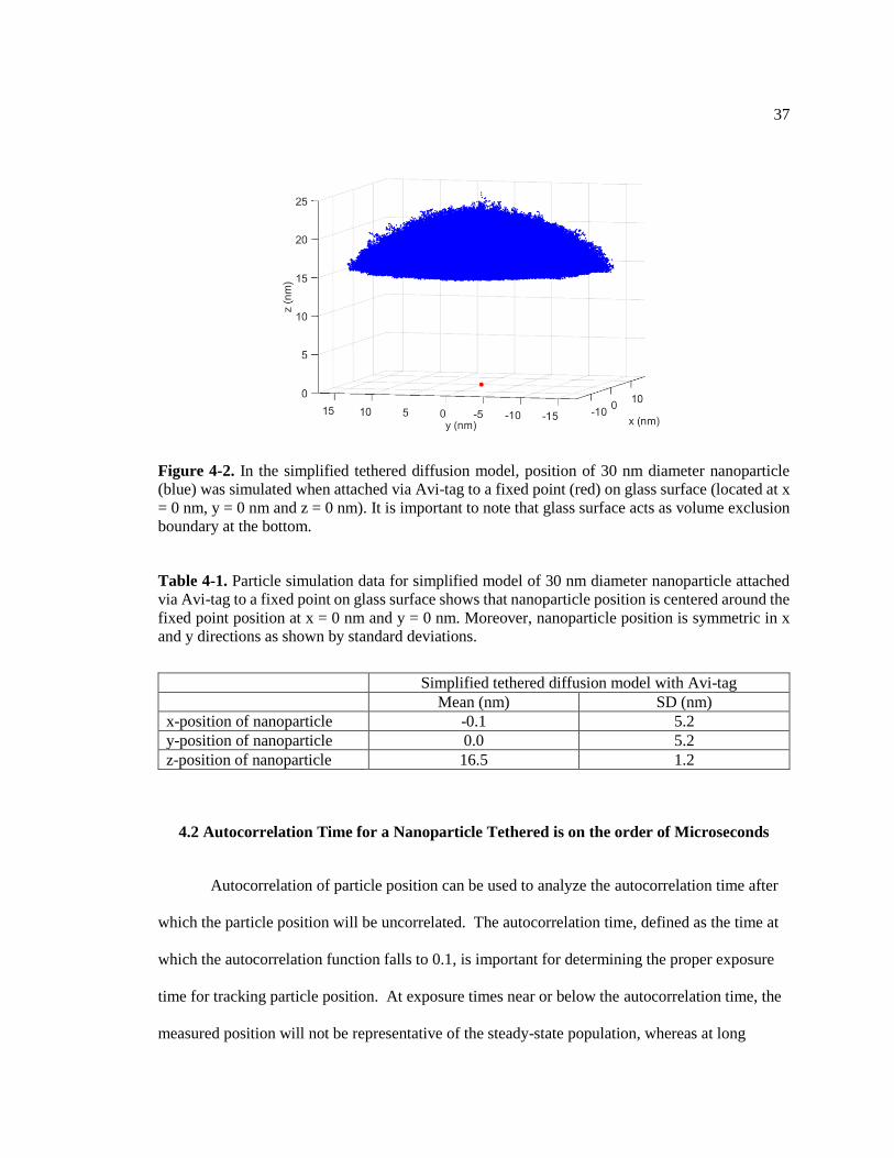
Figure 4-2. In the simplified tethered diffusion model, position of 30 nm diameter

nanoparticle (blue) was simulated when attached via Avi-tag to a fixed point (red)

on glass surface (located at x = 0 nm, y = 0 nm and z = 0 nm). It is important to note

that glass surface acts as volume exclusion boundary at the bottom. .............................. 37

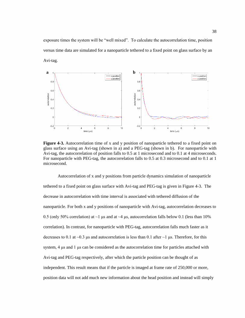
Figure 4-3. Autocorrelation time of x and y position of nanoparticle tethered to a fixed

point on glass surface using an Avi-tag (shown in a) and a PEG-tag (shown in b).

For nanoparticle with Avi-tag, the autocorrelation of position falls to 0.5 at 1

microsecond and to 0.1 at 4 microseconds. For nanoparticle with PEG-tag, the

autocorrelation falls to 0.5 at 0.3 microsecond and to 0.1 at 1 microsecond. .................. 38

Figure 4-4. RMS error vs exposure time from simulation, in which tethered diffusion of

30 nm diameter nanoparticle attached to fixed point on glass surface using a tether

with 1 nm persistence length was imaged at frame rate of 1000 frames/s without any

added image noise. As contour length of the tether increases, RMS error in x

direction increases for all exposure times. For each case, the RMS error decreases

with exposure time and seems to converge to similar value. ........................................... 40

ix

Figure 4-5. RMS error vs exposure time from simulation, in which tethered diffusion of a

30 nm diameter nanoparticle attached to a fixed point on glass surface using a tether

with 11.4 nm contour length was imaged at a frame rate of 1000 frames/s without

any added image noise. As persistence length increases, RMS error in x direction

increases very little. For each case, the RMS error decreases with exposure time but

little difference is observed in RMS error between stiff and compliant tethers. .............. 41


nanoparticle attached to fixed point on a glass surface using a tether with 1 nm

persistence length and 11.4 nm contour length was imaged at frame rate of 1000

frames/s without any added image noise. As nanoparticle size increases, RMS error

in x direction increases drastically for all exposure times. The RMS error decreases

drastically with exposure time, except for 5 nm particle, which shows that for some

particles, exposure time does not change imaging error. ................................................. 42

Figure 4-7. Particle traces for a stationary nanoparticle (a), a nanoparticle tethered to a

moving point on a glass surface via an Avi-tag (b) , and a nanoparticle tethered to a

moving point on a glass surface via a PEG-tag (c). The tether attachment point steps

with step size of 8 nm at frequency of 100 Hz. Traces were generated using

simulation of imaging with 50 frames at frame rate of 1000 fps and exposure time of

0.99 ms. ............................................................................................................................ 44

Figure 4-8. The x-position vs. time traces of Avi-tag (a) and PEG-tag (b) show that a

nanoparticle follows the tether attachment point on a glass surface as it is moved

with step size of 8 nm at frequency of 100 Hz. The y-position vs. time particle traces

for Avi-tag (c) and PEG-tag (d) show large fluctuations in lateral direction due to

tethered diffusion and error associated with imaging process. ........................................ 45

x

LIST OF TABLES

Table 3-1. Particle dynamics simulation data for Avi-tag and PEG-tag when labeled head

is bound (n = 106 points) shows that a nanoparticle with Avi-tag is more accurate

than that with a PEG-tag in x-direction (along the microtubule), but a nanoparticle

with Avi-tag shows rightward bias in y-direction (perpendicular to the microtubule) .... 25

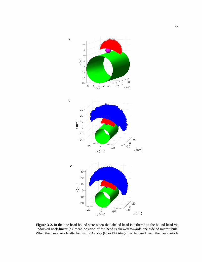
Table 3-2. Particle dynamics simulation data for Avi-tag and PEG-tag when the labeled

head is tethered to the bound head with an undocked neck-linker (n = 106 points)

shows that particles attached with the Avi-tag and the PEG-tag are not very accurate

in the x-direction (along the microtubule) and have rightward bias in y-direction

(perpendicular to the microtubule). The PEG-tag creates much larger force in neck-

linkers than in Avi-tag. ..................................................................................................... 28

Table 3-3. Particle dynamics simulation data for Avi-tag and PEG-tag when labeled head

is tethered to bound head with docked neck-linker (n = 106 points) ................................ 31

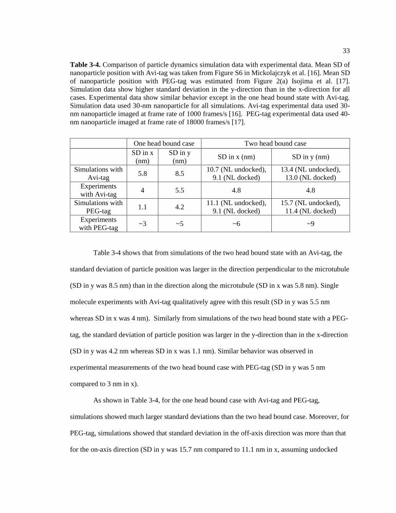
Table 3-4. Comparison of particle dynamics simulation data with experimental data.

Mean SD of nanoparticle position with Avi-tag was taken from Figure S6 in

Mickolajczyk et al. [16]. Mean SD of nanoparticle position with PEG-tag was

estimated from Figure 2(a) Isojima et al. [17]. Simulation data show higher standard

deviation in the y-direction than in the x-direction for all cases. Experimental data

show similar behavior except in the one head bound state with Avi-tag. Simulation

data used 30-nm nanoparticle for all simulations. Avi-tag experimental data used 30-

nm nanoparticle imaged at frame rate of 1000 frames/s [16]. PEG-tag experimental

data used 40-nm nanoparticle imaged at frame rate of 18000 frames/s [17]. .................. 33

Table 4-1. Particle simulation data for simplified model of 30 nm diameter nanoparticle

attached via Avi-tag to a fixed point on glass surface shows that nanoparticle

position is centered around the fixed point position at x = 0 nm and y = 0 nm.

Moreover, nanoparticle position is symmetric in x and y directions as shown by

standard deviations. .......................................................................................................... 37

Table 4-2. Addition of image noise increases RMS error in x and y for fixed

nanoparticle, and nanoparticle tethered with Avi-tag and PEG-tag. Without image

noise, PEG-tag is more accurate at tracking the tether attachment point. But with

image noise, both PEG-tag and Avi-tag give RMS error of approximately 1.6-2 nm ..... 46

xi

ACKNOWLEDGEMENTS

I would like to express my sincere gratitude towards my advisors Dr. William O.

Hancock and Dr. John Fricks for their continuous support, guidance, patience, motivation and

immense knowledge. I would also like to thank Keith Mickolajczyk for experimental data and

guidance for this project. Finally, I would like to thank David Arginteanu, Geng-Yuan Chen and

all other lab members for their valuable input.

1

Chapter 1

Introduction

Kinesins are motor proteins that perform essential functions in cells such as intracellular

transport, microtubules steering and cell division. The kinesin superfamily consists of 45 motor

proteins in humans that can be grouped into 14 families based on their sequence and functions

[1].

1.1 Functions of Kinesins

Transport kinesin, such as those from the kinesin-1 family bind to specific cargo such as

vesicles, organelles and proteins, and transport them along axonal and dendritic microtubules [2].

Cargos are generally simultaneously bound to plus-end-directed kinesin motors responsible for

anterograde transport towards the cell periphery and minus-end-directed dynein motors

responsible for retrograde transport back to the cell body [3]. The bidirectional transport of cargo

is important to understand due to its potential role in neurodegenerative diseases. Alzheimer’s

disease, for example, is characterized by tangles of the microtubule-associated protein tau13 that

inhibit axonal transport. Amyotrophic lateral sclerosis, Huntington’s disease and Parkinson’s

disease are all thought to involve deterioration in anterograde and/or retrograde axonal

transport[4][5][6][7][8].

Kinesins also help in steering microtubule growth in dendrites by actively directing

growing plus-ends of microtubule towards the cell body. A complex of the microtubule plus-end

tracking protein EB1 and the motor Kinesin-2 was shown to direct microtubules growth in vitro,

2

which may explain the uniform minus-end out orientation of microtubules in Drosophila

dendrites [9].

In addition to transport, some kinesins also influence microtubules dynamics along with

microtubule and chromosome movements during mitosis. For instance, Drosophila kinesin-13

members have been shown to drive microtubule depolymerization in interphase cells [10].

Kinesin-5 motors also play a role in cell division by generating forces between overlapped

interpolar microtubules to push mitotic spindle poles apart during anaphase [11]. This function

has made Kinsin-5 a target for potential anticancer chemotherapeutic drugs [12]. Hence,

understanding Kinesin dynamics and the motors’ underlying mechanochemical cycle is important

for the development of future cancer treatments as well.

1.2 Structure of Kinesin-1

Kinesin-1, studied in the present research, contains two 110 kDa heavy chains that

consist of the N-terminal motor head, the flexible neck linker domain, the coiled-coil stalk, and

the C-terminal cargo-binding tail as shown in Figure 1-1. The head domain attaches to tubulin

dimers in microtubule. The tail domain binds to different types of cargo such as vesicles and

protein complexes. Each neck-linker is a 14 amino acid domain that provides flexible connection

between coiled-coil stalk and head domain.

3

Figure 1-1. Kinesin-1 is a dimer with each monomer having a microtubule-binding head domain

connected via flexible neck-linker to coiled-coil stalk, which ends in a cargo-binding tail domain.

Figure adapted from Asbury et al. [13]

Upon ATP binding, the neck linker transitions from a flexible unstructured state to a

structured docked state. Docking of neck linker provides the principal conformational change in

Kinesin to drive it forward as it provides a forward (plus-ended) bias to the motor and enables the

free head to diffuse to the next binding site approximately 8 nm away [14]. During this diffusive

search, the neck linker serves as a tether that constrains the search of the motor head for the next

microtubule binding site and ensures that that lateral or backward steps are exceedingly rare [15].

1.3 Mechanochemical Cycle of Kinesin-1

The kinetic model for the kinesin-1 hydrolysis cycle that underlies this work is presented

in Figure 1-2. This model is built on a large body biophysical and biochemical studies of kinesin.

In the model the motor starts in State 2 with one head bound and undocked neck-linker, which

4

allows the tethered head to bind to either the next binding site or its previous binding site on the

microtubule. ATP binding causes docking of the neck linker domain, which leads to displacement

of the tethered head towards plus-end of the microtubule (State 3). After ATP hydrolysis (State

4), the tethered head can bind to the next binding site on the microtubule (State 1) or, the bound

head can detach before attachment of tethered head (State 5), terminating the run. [15]

Figure 1-2. Simplified mechanochemical cycle of kinesin-1. Figure adapted from Kutys et al [15]

5

1.4 Single Molecule Experiments with Avi-tagged kinesin-1

The following experiment was carried out by Keith Mickolajczyk, a Ph.D. student in the

Hancock lab. Direct observation of the stepping cycle of kinesin-1 was made at saturating ATP

by performing in vitro single-molecule assays under Interferometric scattering (iSCAT)

microscopy as shown in Figure 1-3[16]. Drosophila kinesin-1 (k560) was fused to an N-terminal

Avi-tag and conjugated to a 30 nm streptavidin-coated gold nanoparticle. N-terminal Avi-tag was

attached to the cover strand, which adds additional length to the tag. It is also important to note

that N-terminal Avi-tag came out of right side of the head. Microtubules were attached to a glass

coverslip using rigor kinesins, and the position of the nanoparticles position was imaged with

iSCAT microscopy. A schematic of the experimental setup is shown in Figure 1-3(a). The point-

spread function of gold nanoparticle is shown in Figure 1-3 (b) and sample particle traces are

shown in Figure 1-3(c). [16]

Figure 1-3. Experimental setup of a single molecule experiment with 30 nm diameter gold

nanoparticle attached via Avi-tag to N-terminal of kinesin-1 head is shown in (a). Point spread

function of the gold nanoparticle from interferometric scattering (iSCAT) microscopy is shown in

(b). Sample particle tracks from the single molecule experiments are given in (c), which clearly

show 16.4 nm steps. Figure adapted from Mickolajczyk et al. [16]

From these single molecule experiments, substeps were observed that corresponded to

bound and unbound states of the labeled head as shown in Figure 1-4. The duration of bound state

6

of labeled head was longer than that of unbound state as it includes the duration of two head

bound state of labeled head as well as the duration of one head bound state of unlabeled head.

One head bound state showed a rightward bias of the nanoparticle compared with a two head

bound state. It was discovered that at saturating ATP, kinesin-1 spends half of its chemical cycle

in the one head bound state and the other half in the two head bound state. Also, ATP binding

was found to be necessary to properly enter the one-head bound state and ATP hydrolysis was

required to exit it.

Figure 1-4. Sample particle trace shows that a long bound state of labeled head (black) and a short

unbound state of labeled head (red) was observed in single molecule experiments of tracking of

kinesin-1 head using gold nanoparticle attached with an Avi-tag. Unbound state showed a rightward

bias. Figure adapted from Mickolajczyk et al. [16]

1.5 Single Molecule Experiments with PEG-tagged kinesin-1

Similar to experiments in the Hancock lab, in the Tomishige lab in vitro single molecule

assays were carried out by imaging gold nanoparticle attached to Kinesin-1 head under

microscope [17]. Heterodimeric human kinesin-1 was fused to biotin-PEG2-maleimide tag (PEG-

tag) at single cysteine residue S55C and conjugated to a 40 nm diameter streptavidin-coated gold

nanoparticle. Microtubules were fixed to a glass coverslip, and the position of the nanoparticles

7

position was imaged with total internal reflection (TIRF) dark-field microscopy. A schematic of

the experimental setup is shown in Figure 1-5.

Figure 1-5. Experimental setup of single molecule experiment with 40 nm diameter gold

nanoparticle attached via Avi-tag to S55C residue (located towards minus-end) of kinesin-1 head.

Figure adapted from Isojima et al. [17]

In these experiments, substeps corresponding to bound and unbound states of the labeled

head were also observed as shown in Figure 1-6(a). The one head bound state showed a rightward

bias of nanoparticle compared with the two head bound state, similar to Avi-tag experiments.

8

Figure 1-6. A long bound state of labeled head (red) and a short unbound state of labeled head

(blue) were observed in single molecule experiments of tracking of kinesin-1 head using gold

nanoparticle attached with a PEG-tag. Unbound head showed rightward bias. On-axis and off-

axis displacement traces are shown in (a) and a sample trace is shown in (b). [17]

1.6 Goals of Simulation

There are three major goals of this research – (1) to understand whether attaching gold

nanoparticles with Avi-tag or PEG-tag can perturb natural head dynamics, (2) to evaluate whether

gold nanoparticles with Avi-tag and PEG-tag can accurately track mean head position (without

imaging), and (3) to quantify the effect of different experimental parameters on the accuracy of

gold nanoparticle tracking of a fixed point (with imaging).

For the first two goals, particle dynamics simulations were carried out for various cases.

Two head bound simulations show that Avi-tag is better at tracking bound head than PEG-tag

9

along microtubule direction. One head bound simulations for both undocked and docked neck-

linker conformations show that both Avi-tag and PEG-tag display similar accuracy of tracking

but generate larger force in neck-linker than natural case. Mean force caused by PEG-tag is about

twice as much as that caused by Avi-tag.

For the third goal, position of nanoparticle tethered to a fixed point on a glass surface was

simulated. RMS error in particle position from the fit was chosen as the measure of accuracy of

tracking. First, without adding image noise, effect of different particle sizes, and contour lengths

as well as persistence lengths of tether on the RMS error of tracking was evaluated. Contour

length of tether and particle size had major effects on accuracy of tracking, but persistence length

was found to have the least impact. Then image noise was added and accuracy of PEG-tag and

Avi-tag was compared. But both of them showed similar accuracy, which shows that image noise

was the limiting factor.

10

Chapter 2

Methods

In vitro single molecule experiments of kinesin-1 head allow observation of the motion of

a kinesin-1 head as it moves along the microtubule. But particle dynamics simulations are

required to understand the underlying dynamics of tethered diffusion of head and nanoparticle. In

addition, simulation of imaging process can help us understand the effect of image noise as well

as other experimental factors on accuracy of tracking.

In this study, Monte Carlo simulations in MATLAB® programming language were run

to understand Brownian dynamics of kinesin-1 head and nanoparticle in three dimensions at sub-

nanometer spatial resolution and nanosecond temporal resolution. In addition, the imaging

process was simulated in MATLAB® by superimposing point spread functions to subsampled

nanoparticle position data, calculating average intensity values for each pixel, adding Gaussian

and shot noise to make simulated movies, similar to the ones generated in single molecule

experiments. These simulated movies were then used to fit tracks of particles using the same

program used to fit movies from experiments.

11

2.1 Computational Flowchart

Figure 2-1. Computational flowchart, which includes particle dynamics simulation to generate

simulated particle positions, which were then subsampled and used to make simulated movies.

These simulated movies were used to fit particle traces to get measured particle position data, which

can then be used to compute error statistics

To simulate the gold nanoparticle tracking experiments, first particle dynamics were

simulated for a simplified computational model using Monte Carlo simulation in MATLAB®

with a 1 ns time step. This position data (𝑥𝑠𝑖𝑚𝑢𝑙𝑎𝑡𝑒𝑑 , 𝑦𝑠𝑖𝑚𝑢𝑙𝑎𝑡𝑒𝑑 , 𝑧𝑠𝑖𝑚𝑢𝑙𝑎𝑡𝑒𝑑) was used to

understand the overall distribution of nanoparticle and head position in different

mechanochemical states of the kinesin cycle. Then this position data was subsampled at a rate

that is scaled according to exposure time of the imaging process so that each frame contains at

least 300 points (for instance, with 0.99 ms exposure time, position data would be collected every

3.3 μs). This subsampling rate ensured similar results as that obtained by maximum sampling

while decreasing computation time for simulation of the imaging process. The subsampled data

(𝑥𝑠𝑢𝑏𝑠𝑎𝑚𝑝𝑙𝑒𝑑, 𝑦𝑠𝑢𝑏𝑠𝑎𝑚𝑝𝑙𝑒𝑑) was used to make simulated movies by superimposing a point spread

12

function represented by a 2D Gaussian distribution. Gaussian noise and shot noise were added to

each frame. The frames were stacked to make simulated movies. These movies were used to fit

particle traces (𝑥𝑚𝑒𝑎𝑠𝑢𝑟𝑒𝑑 , 𝑦𝑚𝑒𝑎𝑠𝑢𝑟𝑒𝑑) using Fluorescent Image Evaluation Software for Tracking

and Analysis (FIESTA) program [18] in MATLAB®, which is also used to fit particle traces for

experimental movies. Finally, statistics such as RMS error were calculated by comparing

measured particle position to its mean position of the tether attachment point.

2.2 Particle Dynamics Simulation

2.2.1 Computational Model for Gold Nanoparticle Tracking Experiment

The three-dimensional model used for simulation of single molecule experiments with

gold-nanoparticle using a tag on one of the kinesin-1 heads is shown in Figure 2-2. A number of

assumptions were made to simplify the biomechanical system. The microtubule was modelled as

a cylinder with 25 nm diameter. The microtubule was assumed to be rigidly attached to a glass

surface with rigor kinesins. Tubulin dimers were assumed to be 8 nm apart as kinesin-1 steps are

measured to be 8 nm apart[19]. The gold nanoparticle was assumed to be a sphere with 30 nm

diameter[16], and any radius added by the attached streptavidin was ignored. The kinesin-1

heads, which are dimensions 4.5 x 7 x 4.5 nm [20] were assumed to be spheres with 5 nm

diameter for simplicity. The neck-linkers and Avi-tag were modelled as thermodynamic springs

using the worm-like chain model with persistence length of 1 nm[21]. Contour length of Avi-tag

was calculated to be 11.4 nm as contour length of each amino acids is 0.38 nm [15] and total

number of amino acids is 30, which includes 14 amino acids in Avi-tag sequence[16], 3

glycines[16] and 13 amino acids in N-terminal cover strand [22]. The PEG-tag was also modelled

as a worm-like chain with persistence length of 0.38 nm [23] and contour length of 2.91 nm [24].

13

The coiled-coil stalk was ignored as it does not contribute significantly to the motion of Avi-N

gold nanoparticle.

Note that the positive x-axis points in the direction of microtubule, the positive y-axis is

perpendicular to the microtubule axis and points towards left side of the microtubule, and the

positive z-direction points vertically upwards. The origin of coordinate system was defined such

that center of the bound head is generally located at x = 0 nm, y = 0 nm and z = 2.5 nm.

Figure 2-2. Three-dimensional model used for simulation of single molecule experiments. A 30-

nm gold nanoparticle was attached to kinesin-1 at N-terminal of one of its heads using an Avi-tag.

The tethered kinesin-1 was attached to the bound head through both 14 amino acid neck linker

domains, and the particle and tethered head diffused in three dimensions. The microtubule was

modeled as a 25 nm diameter cylinder. Volume exclusion was maintained in the simulation for the

particle, heads and microtubule, but collisions of the tether with any objects was ignored.

14

2.2.2 Equation of Motion – Langevin Equation

To derive the equation of motion, consider a spherical particle undergoing simple

tethered diffusion in one dimension as shown in Figure 2-3. It experiences three major forces – a

spring force from the tether, random Brownian forces due to diffusion, and a drag force.

Figure 2-3. Free body diagram for simple tethered diffusion of a particle in one dimension. Note

that random Brownian force can act in both directions and drag force always points in the direction

opposite to net velocity.

Using a 30 nm particle moving at velocity of 800 nm/s in water, the Reynolds number is

calculated to be 2.7 x 10-8. At this very low Reynolds number, viscous drag force dominates and

inertial force is negligible. This fact is used to derive overdamped Langevin equation (Equation

5) [15] in one dimension as demonstrated below:

𝐹𝑑𝑖𝑓𝑓𝑢𝑠𝑖𝑜𝑛 + 𝐹𝑠𝑝𝑟𝑖𝑛𝑔 − 𝐹𝑑𝑟𝑎𝑔 = 𝑚𝑎 = 0 (1)

𝐹𝑑𝑟𝑎𝑔 = 𝐹𝑑𝑖𝑓𝑓𝑢𝑠𝑖𝑜𝑛 + 𝐹𝑠𝑝𝑟𝑖𝑛𝑔 (2)

𝜁 𝛥𝑥

𝛥𝑡= 𝐹𝑑𝑖𝑓𝑓𝑢𝑠𝑖𝑜𝑛 + 𝐹𝑠𝑝𝑟𝑖𝑛𝑔 (3)

𝑥𝑖 = 𝑥𝑖−1 + √2𝐷𝑑𝐵(𝑡) +𝛥𝑡

𝜁 𝐹𝑠𝑝𝑟𝑖𝑛𝑔 (4)

𝑥𝑖 = 𝑥𝑖−1 + √2𝐷𝛥𝑡 𝑁(0,1) +𝛥𝑡

𝜁 𝐹𝑠𝑝𝑟𝑖𝑛𝑔 (5)

(Overdamped Langevin equation in one dimension)

15

where 𝜁 = 6𝜋𝑟𝜇 (6)

and 𝐷 =𝑘𝐵𝑇

𝜁

(7)

(𝜁 is viscous drag coefficient, D is diffusion coefficient, 𝑘𝐵 is Boltzmann constant, 𝑇 is

temperature in K, B(t) is Weiner process representing diffusion, and N(0,1) is normal

random number with mean = 0 and SD = 1)

Drag coefficient for a sphere varies according to its distance from a surface as described

by Faxen’s Law shown in Equation 8. From experiments, it has been found that the mean height

of bottom of a microtubule attached to kinesin heads on a glass surface is about 17 nm above the

glass surface[25]. The error between drag coefficients calculated by Equation (6) and Equation

(8) for 30 nm nanoparticle at mean height of 20 nm above the top surface of microtubule, and

hence at height of 62 nm above glass surface (which includes elevation of the microtubule above

the surface, diameter of the microtubule and height of particle above the top surface of

microtubule), was calculated to be 16%. Therefore, approximation from Equation (6) was used to

calculate the drag coefficient instead of Equation (8).

𝜁 =6𝜋𝑟𝜇

1 −9

16(

𝑟ℎ

) +18

(𝑟ℎ

)3

−45

256(

𝑟ℎ

)4

−1

16(

𝑟ℎ

)5 (8)

Faxen’s law for drag on a sphere near a surface

where 𝑟 is radius of the sphere and ℎ is height of the particle above the surface.

2.2.3 Modelling Polypeptides as Entropic Springs using Worm-like Chain Model

The worm-like chain model is the best model currently available to describe entropic

springs such as polypeptide chains and is commonly used to model DNA[26]. Two important

parameters that affect force produced by the spring in this model are contour length and

persistence length. Contour length is the maximum length the tether can be stretched. Persistence

16

length is a measure of compliance of the spring. The force of a worm-like chain is given by

Equation 9 below [15]:

𝐹𝑠𝑝𝑟𝑖𝑛𝑔 =𝑘𝐵𝑇

4𝐿𝑝[(1 −

𝑥 − 𝑥0

𝐿𝑐)

−2

−1

4+

𝑥 − 𝑥0

𝐿𝑐 ] (9)

Worm-like chain equation

where 𝐿𝑝 = persistence length, 𝐿𝑐 = contour length and 𝑥0 = mean position

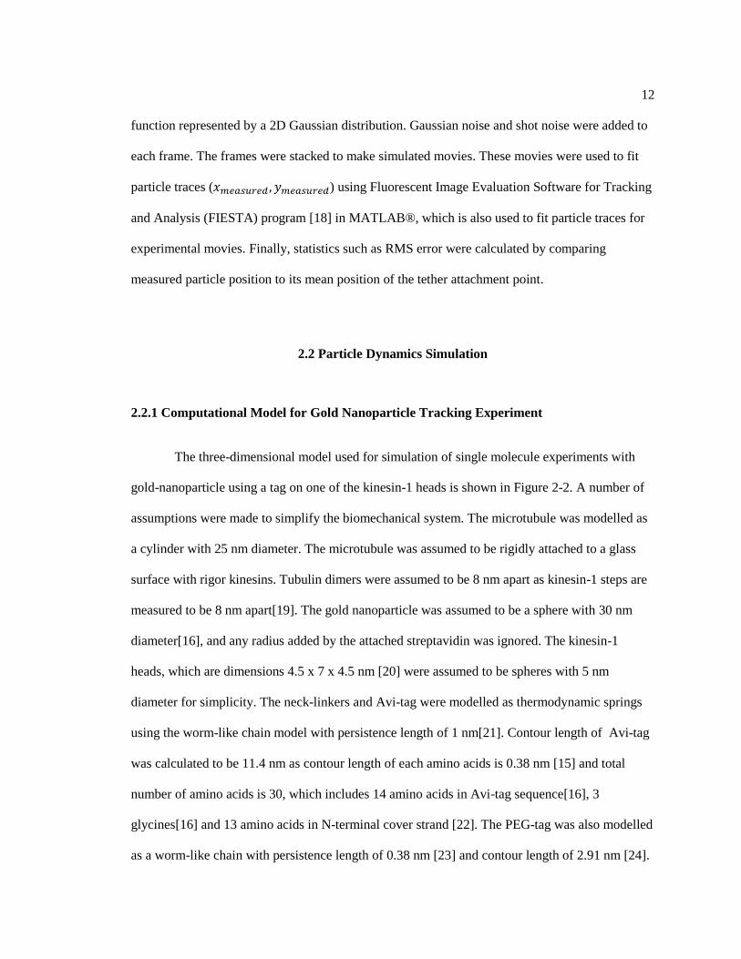
The force-extension curve for kinesin-1 neck linker domain was simulated using

Molecular Dynamics simulation by Hariharan and Hancock [27] and shown to be well fit by a

worm-like chain model with persistence length of 0.5 nm and contour length of 0.38 nm for 15

residue neck-linker is shown in Figure 2-4.

Figure 2-4. Force-extension profile for kinesin-1 neck-linker. Solid curve is prediction from worm-

like chain model for 15 residue peptide with 0.5 nm persistence length and 0.38 nm per residue

contour length. Figure adapted from Hariharan et al. [27]

The worm-like chain formula given comes from an empirical fit to force-extension curve

for many polypeptide chains. It is used here to calculate force generated in neck-linkers and Avi-

17

tag. For kinesin-1 neck-linker, the persistence length is thought to be in range of 0.7 nm to 2 nm

[27]. In this simulation, Avi-tag and both neck-linkers are assumed to have persistence length of 1

nm. Contour length of each amino acid is approximated as 0.38 nm [15]. The PEG-tag was assumed

to have persistence length of 0.38 nm [23] and contour length of 2.91 nm [24]. A ceiling of 100 pN

is put on calculated forces to prevent unnaturally large fluctuations in particle position.

2.2.4 Volume Exclusion for Particle Collisions

Volume exclusion means that two particles cannot occupy the same space at the same

time. Therefore, it is important to include volume exclusion for tethered diffusion simulations to

account for particle collisions [28]. In this study, volume exclusion is considered for collisions

between nanoparticle, kinesin-1 heads, microtubule, and glass surface. Rebounds from particle

collisions are modelled in a simple way – if the calculated position of a particle is inside a volume

exclusion boundary by some distance, the particle rebounds by that distance. For instance, if there

is a surface at z = 0 nm and z-position of the particle calculated from Langevin equation is -2 nm,

then updated z-position of the particle will be z = 2 nm. Surface of the bound head, microtubule

and glass surface at bottom of the microtubule are considered as such volume exclusion

boundaries. For the special case when nanoparticle collides with unbound head, nanoparticle is

moved rather than the head because sometimes head can get stuck bouncing between nanoparticle

and microtubule. Volume exclusion of tethers with any particle or surface were ignored.

2.2.4 Reflective Boundary at Contour Length

Sometimes due to diffusion or volume exclusion, a particle gets beyond its contour

length, which is not possible practically. Therefore, a reflective boundary is put at the contour

18

length of each tether, similar to volume exclusion boundary. If the calculated position of particle

was beyond the contour length of tether by some distance, its position was updated to be contour

length minus that distance.

2.2.5 Implementation in Three Dimensions

Particle position of nanoparticle and head are simulated in three dimensions using the

Langevin equation (Equation 5) and the worm-like chain equation (Equation 9) as follows:

(1) Start with initial condition or previous position in Cartesian coordinates.

(2) Convert Cartesian coordinates to polar coordinates centered at origin of

each tether.

(3) Calculate force in each tether using radial distance.

(4) Adjust radial distance according to the Langevin equation (assuming no

diffusion).

(5) Convert new position of particle from polar coordinates to Cartesian

coordinates.

(6) Add contribution of diffusion along each of the three Cartesian axes.

(7) Check for volume exclusion error between particles or between particles

and microtubule surface in the model, or particle going beyond contour

length error. If any of the errors are true, then repeat checking of errors until

all errors are false.

(8) Save the particle position in Cartesian coordinates and repeat the process

until desired number of iterations.

The head and nanoparticle were assumed to rotate around tether attachment point on their

surface. The length of neck-linkers was assumed to be distance between neck-linker origin on

right surface of the bound head and center of the unbound head minus radius of the unbound

head. For two head bound case, the length of tag was assumed to be distance between neck-linker

19

origin on right surface of the labeled head and center of the nanoparticle minus radius of the

nanoparticle. The position of origin of tag on labeled head surface was not tracked in one head

bound case. Therefore, for one head bound case, the length of tag was assumed to be distance

between center of the labeled and center of the nanoparticle minus radius of the labeled head and

radius of the nanoparticle.

For detailed information about implementation in MATLAB, see sample codes in

Appendix A and Appendix B.

2.3 Subsampling of Particle Position

Particle dynamics simulation data was recorded at time interval of 1 ns. But for

simulation of the imaging process, it was necessary to subsample particle position to increase

speed of the computation. The sampling rate is scaled with exposure time to ensure an equal

number of particle positions used for each frame of the simulated movie regardless of the

exposure time. The imaging simulation was carried out with different subsampling rate, and it

was found that a minimum subsampling rate of 300 points per frame is needed to obtain less than

0.1 nm RMS error compared to maximum subsampling rate. Therefore, this subsampling rate of

300 points per frame is used in imaging simulations.

2.4 Simulation of the Imaging Process

There are two important parameters for the imaging process – frame rate and exposure

time. Frame rate describes frequency of the recording of frames, while exposure time describes

duration of time the shutter is open to record the intensity values. In this study, a frame rate of

1000 frames/s and exposure time of 0.99 ms was used, which is what was used for single

20

molecule experiments with Avi-tag in Hancock lab [16]. It is found in experiments that the point

spread function of fixed gold nanoparticle can be approximated by a two-dimensional Gaussian

function to describe the intensity with full-width half-max of 275 nm [16]. Frame size of 30 x 30

pixels with pixel length of 31.8 nm was used.

A simulated movie is made from subsampled data using the following procedure:

(1) Two-dimensional Gaussian point-spread function is superimposed on each

subsampled position data point.

(2) Average intensity of the 2D Gaussian in each pixel is calculated by

integrating the 2D Gaussian in the pixel and dividing by area of the pixel.

Integration of 2D Gaussian between points (q,r) and (s,t) is calculated using

cumulative density function using the following formulae:

∫ ∫ 𝑓(𝑢, 𝑣)𝑑𝑢𝑑𝑣𝑡

𝑟

𝑠

𝑞

= ∫ ∫ 𝑓(𝑢, 𝑣)𝑑𝑣𝑑𝑢𝑡

−∞

𝑠

−∞

− ∫ ∫ 𝑓(𝑢, 𝑣)𝑑𝑣𝑑𝑢𝑟

−∞

𝑠

−∞

− ∫ ∫ 𝑓(𝑢, 𝑣)𝑑𝑣𝑑𝑢𝑡

−∞

𝑞

−∞

+ ∫ ∫ 𝑓(𝑢, 𝑣)𝑑𝑣𝑑𝑢𝑟

−∞

𝑞

−∞

(10)

∫ ∫ 𝑓(𝑢, 𝑣)𝑡

𝑟

𝑠

𝑞

= F(s, t) − F(s, r) − F(q, t) + F(q, r) (11)

Because of independence, F(𝑠, 𝑡) = Φ(𝑠)Φ(𝑡) (12)

where Φ(𝑠) = ∫1

√2𝜋

𝑠

−∞𝑒−𝑢2/2𝑑𝑢 (13)

Formulae for integration of 2D Gaussian point spread function using cumulative

density function

(3) Intensity values from all 2D Gaussians corresponding to subsampled particle

positions within the exposure time of the frame are added together.

(4) All intensity values are converted to 16-bit values and are scaled by one-

fourth to ensure that the frame is not oversaturated.

21

(5) Shot noise from the camera generally follows Poisson distribution [29]. So,

for each pixel, the new intensity value is chosen from a Poisson distribution with

mean and standard deviation equal to the intensity value calculated from the

previous step.

(6) Background is assumed to be Gaussian noise with mean of 0. A standard

deviation of 1300 for 16-bit image was found to give standard deviation of ~2 nm

for stationary nanoparticle similar to experimental results. Therefore, Gaussian

noise with mean of 0 and standard deviation of 1300 is added to each pixel.

(7) Frames thus obtained are stacked and saved as a simulated movie. A sample

frame for imaging of stationary nanoparticle with added noise is shown in Figure

2-5.

For detailed information about implementation of imaging simulation in MATLAB, see

Appendix C.

Figure 2-5. Sample frame from simulation of imaging a fixed nanoparticle with added shot noise

and Gaussian background noise

2.5 Fitting of Particle Tracks

The simulated movie was fit with Fluorescence Image Evaluation Software for Tracking

and Analysis (FIESTA) program in MATLAB® – the same program used to fit particle tracks for

22

single molecule movies in Hancock lab [18]. The intensity threshold was set at 1200. This

automated program uses 2D Gaussian model to fit particle position with about one-nanometer

precision [18].

2.6 Calculation of Statistics

For the particle dynamics simulation data for Chapter 3, statistics calculated were mean

and standard deviation of head and nanoparticle position, and of forces in neck-linkers and Avi-

tag or PEG-tag. To calculate accuracy of tracking for imaging simulations for Chapter 4, RMS

error was calculated, which is defined as root-mean-square error between measured particle

position and its true mean position, i.e., position of tether attachment point on the glass surface.

For the imaging simulation, it was found that when no noise is added, measured particle

position for a particular frame can be calculated directly by averaging subsampled position data

within exposure time of the frame. This result means if a 2D Gaussian is fit to a sum of 2D

Gaussians, it approximates the mean of centers of 2D Gaussians very well. This fact was used to

simplify simulation of imaging process when no noise was added.

23

Chapter 3

Particle Dynamics Simulation of Single Molecule Experiments with Avi-tag

and PEG-tag

3.1 Two Head Bound Case

To characterize the effects of attachment tether just on nanoparticle position, simulations

were carried out for “two head bound case”, in which the labeled head is bound to the

microtubule. Two conditions were studied – gold nanoparticle attached with Avi-tag and with

PEG-tag. Position data were simulated for total time of 1 ms (106 points at 1 ns time step).

Results are shown in Figure 3-1 and Table 3-1.

24

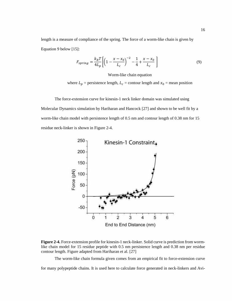
Figure 3-1. In the two head bound state when the labeled head is bound to the microtubule, the

nanoparticle attached via Avi-tag (shown in a) samples significantly larger volume than that via

PEG-tag (shown in b). The nanoparticle with Avi-tag tends to stay on the right side of the

microtubule. Positions are plotted at an interval of 1 ns for a total period of 1 ms. The labeled head

is shown in red and the microtubule is shown in green. The nanoparticle position is shown in blue.

The plus-end of microtubule is towards positive x-axis.

a

b

25

Table 3-1. Particle dynamics simulation data for Avi-tag and PEG-tag when labeled head is bound

(n = 106 points) shows that a nanoparticle with Avi-tag is more accurate than that with a PEG-tag

in x-direction (along the microtubule), but a nanoparticle with Avi-tag shows rightward bias in y-

direction (perpendicular to the microtubule)

Two-head bound state

Avi-tag PEG-tag

Mean SD Mean SD

x-position of nanoparticle (nm) 0.7 5.8 -8.1 1.1

y-position of nanoparticle (nm) -6.5 8.5 0.0 4.2

z-position of nanoparticle (nm) 17.3 2.9 17.7 0.6

Length of attached tether (nm) 4.4 1.4 1.8 0.2

Force in attached tether (pN) 2.8 1.5 23.4 10.2

Figure 3-1 shows that the distribution of nanoparticle position around the microtubule

resembles a saddle shape due to tethered diffusion and volume exclusion due to the presence of

the microtubule. As shown in Figure 3-1 and Table 3-1, the nanoparticle attached via Avi-tag

samples much larger volume around the bound head than particles attached via a PEG-tag (SD in

y-direction of 8.5 nm for Avi-tag and 4.2 nm for PEG-tag). This result is not surprising because

of the difference in contour lengths between the tethers (contour length of Avi-tag is 11.4 nm

compared to 2.91 nm of PEG-tag); the different persistent lengths (persistence length of Avi-tag

is assumed to be 1 nm while that of PEG-tag is 0.38 nm) could also contribute because a smaller

persistence length results in a larger force resisting stretch of the tether. Importantly, the mean

nanoparticle position along the x-direction (along the microtubule axis) was approximately 0 nm

for Avi-tag but was -8 nm for Avi-tag. In the y-direction (perpendicular to the microtubule), mean

nanoparticle position for PEG-tag is 0 nm, but for the Avi-tag it is skewed towards the right side

of the head (mean y-position for Avi-tag is -6.5 nm). Differences in these mean positions is likely

caused due by differences in location of origin tethers on labeled head surface. Avi-tag was

assumed to come out of the right side of the labeled head surface at position of x = 0 nm, y = -2.5

nm and z = 2.5 nm, whereas PEG-tag was assumed to come out of back side of the labeled head

surface at position of x = 0 nm, y = -2.5 nm and z = 2.5 nm. In addition, force produced in the

26

PEG-tag was much higher than that produced by the Avi-tag, which is probably due to

differences in persistence length and contour length between the tethers. Therefore, two head

bound simulation data show that although nanoparticle position for the Avi-tag has a bias towards

the right side of microtubule; it is accurate in the x-direction. In contract, a nanoparticle with

PEG-tag does not have bias perpendicular to microtubule, but does not show the bound head

position accurately along the microtubule as its mean position is very close to the previous

binding site on the microtubule rather than the site where the labeled head is bound.

3.2 One Head Bound Case with Undocked Neck-linker

To understand the effect of attaching a nanoparticle on the natural dynamics of the head,

particle dynamics simulations were performed for “one head bound case”, in which the labeled

head is free to diffuse but is tethered to the unlabeled head. The neck-linker is assumed to be

undocked in this case. Three conditions were studied – no particle attached (i.e. natural state),

nanoparticle attached with Avi-tag, and nanoparticle attached with PEG-tag. Position data were

simulated for a total time of 1 ms (106 points at 1 ns time step). Results are shown in Figure 3-2

and Table 3-2.

27

Figure 3-2. In the one head bound state when the labeled head is tethered to the bound head via

undocked neck-linker (a), mean position of the head is skewed towards one side of microtubule.

When the nanoparticle attached using Avi-tag (b) or PEG-tag (c) to tethered head, the nanoparticle

a

b

c

28

(Figure 3-2 continued) samples larger volume around microtubule than in the two head bound

state, with a bias towards the right side of microtubule. A nanoparticle attached via PEG-tag

samples larger volume than that with Avi-tag. The microtubule is shown in green and bound head

is shown in magenta. Positions of labeled head (red) and nanoparticle (blue) are plotted at interval

of 1 ns for total period of 1 ms. The plus-end of microtubule is towards positive x-axis.

Table 3-2. Particle dynamics simulation data for Avi-tag and PEG-tag when the labeled head is

tethered to the bound head with an undocked neck-linker (n = 106 points) shows that particles

attached with the Avi-tag and the PEG-tag are not very accurate in the x-direction (along the

microtubule) and have rightward bias in y-direction (perpendicular to the microtubule). The PEG-

tag creates much larger force in neck-linkers than in Avi-tag.

One-head bound state with undocked neck-linker

Avi-tag PEG-tag

No nanoparticle

attached

Mean SD Mean SD Mean SD

x-position of nanoparticle (nm) 1.8 10.7 1.8 11.1 n/a n/a

y-position of nanoparticle (nm) -4.7 13.4 -1.9 15.7 n/a n/a

z-position of nanoparticle (nm) 20.5 6.3 19.5 7.5 n/a n/a

Length of attached tether (nm) 3.3 1.7 1.0 0.6 n/a n/a

Force in attached tether (pN) 2.6 2.1 10.1 12.7 n/a n/a

x-position of labeled head (nm) 0.3 3.6 0.6 4.0 0.0 3.1

y-position of labeled head (nm) -3.4 3.9 -2.4 5.4 -4.1 3.0

z-position of labeled head (nm) 7.1 2.1 8.1 2.7 6.2 1.68

Length of neck-linker (nm) 4.7 1.5 6.62 1.1 3.5 1.3

Force in neck-linker (pN) 5.1 3.7 10.8 6.9 2.9 1.7

As shown in Figure 3-2 and Table 3-2, attaching a nanoparticle to the tethered head

decreases the rightward bias of the head in the y-direction (perpendicular to the microtubule),

while keeping approximately the same mean position in the x-direction. The mean nanoparticle

position in x (along the microtubule) was 1.8 nm for both tags, compared to a mean position of 0

nm for the untagged head. This result shows that particles attached using Avi-tag and PEG-tag

are not very accurate in x in one head bound condition with undocked neck-linker. In the y-

direction, both tethers have a rightward bias likely due to the rightward bias in position of the

labeled head. A nanoparticle with PEG-tag shows less rightward bias than Avi-tag, probably due

to the shorter tether length.

29

More importantly, when the neck-linker is undocked, attaching a PEG-tag increases mean

force in neck-linkers from 2.9 pN to 10.8 pN, whereas attaching Avi-tag increases it to only 5.1

pN. This simulation was repeated with 0.1 ns time step instead of 1 ns time step and similar

behavior was observed – an Avi-tag increased the mean force in undocked neck-linkers from 2.9

pN to 4.5 pN, whereas a PEG-tag increases it to about twice the force from 2.9 pN to 9.8 pN.

These data suggest that that a particle attached to a head through a PEG-tag may perturb the

natural mechanochemical cycle of kinesin-1 more than that with Avi-tag by creating large forces

in neck-linkers.

3.3 One Head Bound Case with Docked Neck-linker

Next, particle dynamics simulations were performed for the one head bound state with

docked neck-linker, in which one of the two neck-linker undergoes conformational change,

pushing mean position of the tethered head towards the plus-end of the microtubule. Three

conditions were studied – no particle attached (i.e. natural state), nanoparticle attached with Avi-

tag and nanoparticle attached with PEG-tag. Position data were simulated for a total time of 1 ms

(106 points at 1 ns time step). Results are shown in Figure 3-3 and Table 3-3.

30

Figure 3-3. In one head bound state when the labeled head is tethered to the bound head via docked

neck-linker (a), the mean position of head is skewed towards right side of the microtubule due to

volume exclusion with the bound head and is shifted towards the plus-end due to neck-linker

a

b

c

31

(Figure 3-3 continued) docking. When nanoparticle is attached using Avi-tag (b) or PEG-tag (c)

to the tethered head with docked neck-linker, nanoparticle position shifts in the positive x-direction,

while not retaining a rightward bias. Both tags seem to result in similar nanoparticle position

distribution. Microtubule is shown in green, bound head is shown in magenta and docked part of

neck-linker is shown in black. Positions of labeled head (red) and nanoparticle (blue) at plotted at

interval of 1 ns for total period of 1 ms. Plus-end of microtubule is towards positive x-axis.

Table 3-3. Particle dynamics simulation data for Avi-tag and PEG-tag when labeled head is

tethered to bound head with docked neck-linker (n = 106 points)

One-head bound state with docked neck-linker Avi-tag PEG-tag No tether attached Mean SD Mean SD Mean SD

x-position of nanoparticle (nm) 6.4 9.1 7.1 9.1 n/a n/a

y-position of nanoparticle (nm) -1.2 13.0 1.1 11.4 n/a n/a

z-position of nanoparticle (nm) 19.6 5.0 20.3 4.3 n/a n/a

Length of attached tether (nm) 3.1 1.6 1.0 0.6 n/a n/a

Force in attached tether (pN) 2.3 1.8 9.9 12.3 n/a n/a

x-position of labeled head (nm) 5.8 1.9 5.8 2.2 5.7 1.9

y-position of labeled head (nm) -0.1 2.6 0.2 2.9 -3.3 2.2

z-position of labeled head (nm) 6.2 1.0 6.7 1.2 5.6 1.0

Length of neck-linker (nm) 2.5 1.0 3.2 0.8 1.9 0.9

Force in neck-linker (pN) 7.0 8.6 12.2 13.3 3.7 3.5

As shown in Figure 3-3 and Table 3-3, when neck-linker is docked, attaching tags to

tethered head does not change the mean position of the head in x-direction (along the

microtubule), but decreases its rightward bias in the y-direction. Mean position of the head in the

x-direction (along the microtubule) is 5.8 nm with both Avi-tag and PEG-tag, which is close to

the expected mean value of 5.32 nm. But mean position of the nanoparticle in the x-direction

(along the microtubule axis) is 6.4 nm for Avi-tag and 7.1 nm for PEG-tag compared to mean

position of 5.8 nm of the head, which shows that Avi-tag and PEG-tag are not very accurate in

the x direction in the one head bound condition with a docked neck-linker. In the y-direction

(perpendicular to the microtubule), nanoparticles with tethers do not show much bias towards

either side of the microtubule, which was observed in the case of undocked neck-linker.

32

More importantly, for the docked neck-linker case, attaching a PEG-tag increases mean

force in neck-linker from 3.7 pN to 12.0 pN, whereas attaching Avi-tag increases it to only 6.6

pN. This shows that a PEG-tag may perturb the natural mechanochemical cycle of kinesin-1 by

creating large forces in neck-linkers.

3.4 Comparison of Simulation Data with Experimental Data

Fluctuations in particle position measured in experiments can be due to combination of

different factors – coupled tethered diffusion of nanoparticle and labeled head, spatiotemporal

averaging from imaging process, errors associated with image noise and fitting of traces to

movies. Although these are different measurements, standard deviations in particle position from

tethered diffusion are compared to experimental values in Table 3-4 to see if the overall behavior

of the distribution of particle positions can be explained by tethered diffusion itself. It is

important to note that PEG-tag experiments used 40-nm diameter bead but for simulations, 30-nm

diameter bead is used to compare PEG-tag vs. Avi-tag. Mean SD of nanoparticle position with

Avi-tag was taken from Figure S6 in Mickolajczyk et al. [16]. Mean SD of nanoparticle position

with PEG-tag was estimated from Figure 2(a) Isojima et al. [17].

33

Table 3-4. Comparison of particle dynamics simulation data with experimental data. Mean SD of

nanoparticle position with Avi-tag was taken from Figure S6 in Mickolajczyk et al. [16]. Mean SD

of nanoparticle position with PEG-tag was estimated from Figure 2(a) Isojima et al. [17].

Simulation data show higher standard deviation in the y-direction than in the x-direction for all

cases. Experimental data show similar behavior except in the one head bound state with Avi-tag.

Simulation data used 30-nm nanoparticle for all simulations. Avi-tag experimental data used 30-

nm nanoparticle imaged at frame rate of 1000 frames/s [16]. PEG-tag experimental data used 40-

nm nanoparticle imaged at frame rate of 18000 frames/s [17].

One head bound case Two head bound case

SD in x

(nm)

SD in y

(nm) SD in x (nm) SD in y (nm)

Simulations with

Avi-tag 5.8 8.5

10.7 (NL undocked),

9.1 (NL docked)

13.4 (NL undocked),

13.0 (NL docked)

Experiments

with Avi-tag 4 5.5 4.8 4.8

Simulations with

PEG-tag 1.1 4.2

11.1 (NL undocked),

9.1 (NL docked)

15.7 (NL undocked),

11.4 (NL docked)

Experiments

with PEG-tag ~3 ~5 ~6 ~9

Table 3-4 shows that from simulations of the two head bound state with an Avi-tag, the

standard deviation of particle position was larger in the direction perpendicular to the microtubule

(SD in y was 8.5 nm) than in the direction along the microtubule (SD in x was 5.8 nm). Single

molecule experiments with Avi-tag qualitatively agree with this result (SD in y was 5.5 nm

whereas SD in x was 4 nm). Similarly from simulations of the two head bound state with a PEG-

tag, the standard deviation of particle position was larger in the y-direction than in the x-direction

(SD in y was 4.2 nm whereas SD in x was 1.1 nm). Similar behavior was observed in

experimental measurements of the two head bound case with PEG-tag (SD in y was 5 nm

compared to 3 nm in x).

As shown in Table 3-4, for the one head bound case with Avi-tag and PEG-tag,

simulations showed much larger standard deviations than the two head bound case. Moreover, for

PEG-tag, simulations showed that standard deviation in the off-axis direction was more than that

for the on-axis direction (SD in y was 15.7 nm compared to 11.1 nm in x, assuming undocked

34

neck-linker). Single molecule experiments with PEG-tag show similar asymmetry in standard

deviation (SD in y was approximately 9 nm and SD in x was approximately 6 nm). Similarly,

simulations for one head bound case with Avi-tag showed asymmetry in particle position

distribution (SD in y was 13.4 nm compared to 10.4 nm in x, assuming undocked neck-linker). In

contrast, single molecule experiments with Avi-tag gave similar standard deviation in x and y

directions. This disagreement is likely due to the fact that experimental data includes

spatiotemporal averaging and error associated with image noise, which will be addressed in

Chapter 4.

Therefore, experimental data generally agrees qualitatively with particle dynamics

simulation data. Moreover, the asymmetry in on-axis and off-axis standard deviations in

experimental data for two head bound case can be explained by simulation. This asymmetry is

likely caused by volume exclusion of nanoparticle due to presence of the microtubule surface.

35

Chapter 4

Accuracy of Tracking by Imaging a Gold-nanoparticle

In addition to minimally perturbing the natural system, a nanoparticle should also track

the position of a kinesin head with high accuracy. Accurate tracking requires a sufficient number

of collected photons to fit the point-spread function, and it also requires an exposure time that is

longer than the correlation time of the particle, such that the measured position is representative

of the particle positional distribution. In this chapter, the effects of the experimental factors such

as contour length and persistence length of the nanoparticle tether, and size of nanoparticle were

examined using a simple system of nanoparticle tethered to a fixed point on glass surface. This

geometry was chosen to focus in on the interplay of particle dynamics, exposure time, and frame

rate in the absence of any geometrical factors from the bound head or microtubule.

The work proceeded as follows. First, the effect of experimental parameters was

explored without adding any noise to the imaging process. It was found that without any added

image noise, the measured position in each frame of simulated movie was approximately equal to

the mean position within the exposure time. Therefore, for cases without image noise, the mean

of subsampled position data within exposure time of the frame was used as approximation for the

measured value of particle position from the fit. RMS errors were calculated by comparing this

measured value to fixed point on glass surface where tether is attached, which is its true mean

position. These RMS errors were used to compare accuracy of tracking for different experimental

cases.

36

4.1 Simplified Model of Tethered Diffusion of Nanoparticle

In this chapter, a simple model (shown in Figure 4-1) was used where a nanoparticle is

attached to fixed point on glass surface by a tether such as Avi-tag. This model is supposed to

mimic the two head bound state where a nanoparticle is attached to the bound head on a

microtubule using Avi-tag, but it avoids complicating issues of asymmetry caused by microtubule

geometry. Particle dynamics simulation data of 30 nm gold nanoparticle attached via Avi-tag to a

fixed point on glass surface in this simplified model is shown in Figure 4-2. Glass surface acts as

a volume exclusion boundary at the bottom. It is important to note that position of the

nanoparticle in this tethered diffusion model is symmetric in x and y directions, and is centered

about the tether attachment point as shown in Table 4-1. This simplified tethered diffusion model

is used in following sections to simulate imaging with and without added noise. Without added

noise, spatiotemporal averaging of nanoparticle is used to calculate measured particle position.

With added noise, nanoparticle positions are used to make a simulated movie, which is then fit to

calculate measured particle position.

Figure 4-1. Simplified tethered diffusion model of a 30 nm diameter nanoparticle attached via Avi-

tag to a fixed tether attachment point on a glass surface.

37

Figure 4-2. In the simplified tethered diffusion model, position of 30 nm diameter nanoparticle

(blue) was simulated when attached via Avi-tag to a fixed point (red) on glass surface (located at x

= 0 nm, y = 0 nm and z = 0 nm). It is important to note that glass surface acts as volume exclusion

boundary at the bottom.

Table 4-1. Particle simulation data for simplified model of 30 nm diameter nanoparticle attached

via Avi-tag to a fixed point on glass surface shows that nanoparticle position is centered around the

fixed point position at x = 0 nm and y = 0 nm. Moreover, nanoparticle position is symmetric in x

and y directions as shown by standard deviations.

Simplified tethered diffusion model with Avi-tag

Mean (nm) SD (nm)

x-position of nanoparticle -0.1 5.2

y-position of nanoparticle 0.0 5.2

z-position of nanoparticle 16.5 1.2

4.2 Autocorrelation Time for a Nanoparticle Tethered is on the order of Microseconds

Autocorrelation of particle position can be used to analyze the autocorrelation time after

which the particle position will be uncorrelated. The autocorrelation time, defined as the time at

which the autocorrelation function falls to 0.1, is important for determining the proper exposure

time for tracking particle position. At exposure times near or below the autocorrelation time, the

measured position will not be representative of the steady-state population, whereas at long

38

exposure times the system will be “well mixed”. To calculate the autocorrelation time, position

versus time data are simulated for a nanoparticle tethered to a fixed point on glass surface by an

Avi-tag.

Figure 4-3. Autocorrelation time of x and y position of nanoparticle tethered to a fixed point on

glass surface using an Avi-tag (shown in a) and a PEG-tag (shown in b). For nanoparticle with

Avi-tag, the autocorrelation of position falls to 0.5 at 1 microsecond and to 0.1 at 4 microseconds.

For nanoparticle with PEG-tag, the autocorrelation falls to 0.5 at 0.3 microsecond and to 0.1 at 1

microsecond.

Autocorrelation of x and y positions from particle dynamics simulation of nanoparticle

tethered to a fixed point on glass surface with Avi-tag and PEG-tag is given in Figure 4-3. The

decrease in autocorrelation with time interval is associated with tethered diffusion of the

nanoparticle. For both x and y positions of nanoparticle with Avi-tag, autocorrelation decreases to

0.5 (only 50% correlation) at ~1 μs and at ~4 μs, autocorrelation falls below 0.1 (less than 10%

correlation). In contrast, for nanoparticle with PEG-tag, autocorrelation falls much faster as it

decreases to 0.1 at ~0.3 μs and autocorrelation is less than 0.1 after ~1 μs. Therefore, for this

system, 4 μs and 1 μs can be considered as the autocorrelation time for particles attached with

Avi-tag and PEG-tag respectively, after which the particle position can be thought of as

independent. This result means that if the particle is imaged at frame rate of 250,000 or more,

position data will not add much new information about the head position and instead will simply

a b

39

be measuring the diffusion of the particle. However, the maximum frame rate is limited by the

camera. Generally for single molecule experiments, a nanoparticle is imaged at frame rate

ranging from 1000 fps [16] to 109,500 fps [17]. Even at high frame rate of 109,500 fps,

nanoparticle position will be uncorrelated and can thus be downsampled if necessary.

Autocorrelation time may also be related to how RMS error in particle position changes with

exposure time of imaging process.

4.3 Effect of Contour Length of Attached Tether on RMS Error of Nanoparticle Tracking

Figure 4-4 shows the effect of contour length of tether on RMS error in the x-direction

between a measured value from imaging process without added image noise and a tether

attachment point on glass surface, which is the mean position in x. Imaging simulation is done at

a frame rate of 1000 frames/s. Persistence length of the tether and the diameter of nanoparticle

were kept constant at 1 nm and 30 nm respectively. As exposure time increases, RMS error

decreases because the nanoparticle can sample more points around the mean position. As contour

length of the tether decreases, RMS error increases because a shorter tether allows a nanoparticle

to sample the area around the mean position quickly. Therefore, a shorter tether should be used

for imaging, provided it does not induce large forces in a target like PEG-tag.

40

Figure 4-4. RMS error vs exposure time from simulation, in which tethered diffusion of 30 nm

diameter nanoparticle attached to fixed point on glass surface using a tether with 1 nm persistence

length was imaged at frame rate of 1000 frames/s without any added image noise. As contour length

of the tether increases, RMS error in x direction increases for all exposure times. For each case, the

RMS error decreases with exposure time and seems to converge to similar value.

4.4 Effect of Persistence Length of Attached Tether on RMS Error of Nanoparticle

Tracking

Figure 4-5 shows the effect of persistence length of tether on RMS error in x-direction

between measured value from imaging process without added image noise, and tether attachment

point on glass surface, which is the mean position in x. Imaging simulation is done at frame rate

of 1000 frames/s. Contour length of the tether and nanoparticle diameter were kept constant at

11.4 nm and 30 nm respectively. Data show that as exposure time increases, RMS error decreases

because a nanoparticle can sample more points around mean position. As persistence length

increases, RMS error increases slightly because stiff tethers pull a particle more towards center

41

resulting in smaller RMS error. Although data show that nanoparticle with less compliant tether

seems to be better at tracking the fixed point, overall persistence length does not have as

significant an effect on RMS error as contour length or particle size.

Figure 4-5. RMS error vs exposure time from simulation, in which tethered diffusion of a 30 nm

diameter nanoparticle attached to a fixed point on glass surface using a tether with 11.4 nm contour

length was imaged at a frame rate of 1000 frames/s without any added image noise. As persistence

length increases, RMS error in x direction increases very little. For each case, the RMS error

decreases with exposure time but little difference is observed in RMS error between stiff and

compliant tethers.

4.5 Effect of Particle Size on RMS Error of Nanoparticle Tracking

Figure 4-6 shows the effect of particle size on RMS error in the x-direction between

measured value from imaging process without added image noise, and the tether attachment point

on a glass surface, which is the mean position in x. Imaging simulation is done at a frame rate of

1000 frames/s. Persistence length and contour length of the tether were kept constant at 1 nm and

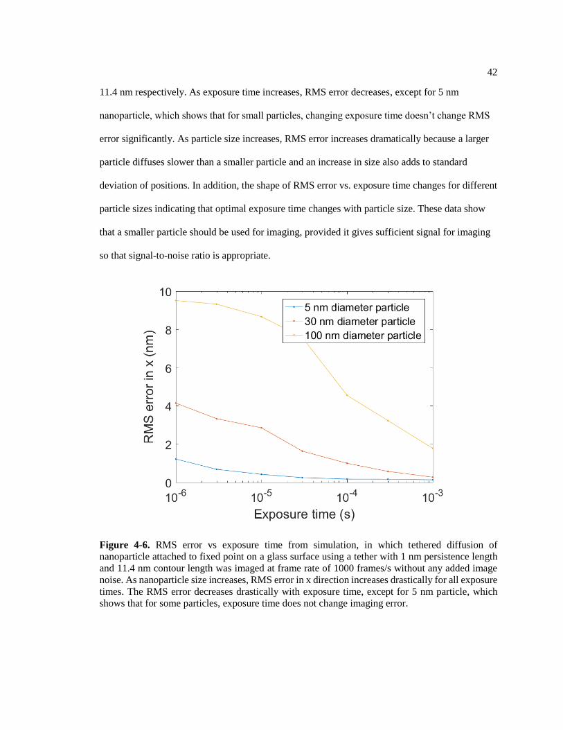
42

11.4 nm respectively. As exposure time increases, RMS error decreases, except for 5 nm

nanoparticle, which shows that for small particles, changing exposure time doesn’t change RMS

error significantly. As particle size increases, RMS error increases dramatically because a larger

particle diffuses slower than a smaller particle and an increase in size also adds to standard

deviation of positions. In addition, the shape of RMS error vs. exposure time changes for different

particle sizes indicating that optimal exposure time changes with particle size. These data show

that a smaller particle should be used for imaging, provided it gives sufficient signal for imaging

so that signal-to-noise ratio is appropriate.


nanoparticle attached to fixed point on a glass surface using a tether with 1 nm persistence length

and 11.4 nm contour length was imaged at frame rate of 1000 frames/s without any added image

noise. As nanoparticle size increases, RMS error in x direction increases drastically for all exposure

times. The RMS error decreases drastically with exposure time, except for 5 nm particle, which

shows that for some particles, exposure time does not change imaging error.

43

4.6 Effect of Image Noise on Accuracy of Nanoparticle with Avi-tag and PEG-tag

First, simulated movie of a stationary nanoparticle was made with 50 frames at a frame

rate of 1000 fps and an exposure time of 0.99 ms to calibrate image noise. Shot noise and

Gaussian noise were added to Gaussian point spread functions of stationary nanoparticle as

described in Chapter 2. Standard deviation of Gaussian noise was chosen so that particle position

from fit has standard deviation of ~2 nm in both directions. A particle trace of this stationary

particle (negative control case) is shown in Figure 4-7 (a).

Then the same image noise values were used to make simulated movies of a tethered

nanoparticle attached to a fixed point on glass surface (true mean position) that is moved with

step size of 8 nm at frequency of 100 Hz similar to stepping of kinesin-1 at 800 nm/s. Frame rate

of 1000 fps is used with exposure time of 0.99 ms, similar to experiments run in Hancock lab.

Particle traces of tethered diffusion of nanoparticle with Avi-tag and PEG-tag are shown in Figure

4-7 (b) and (c), respectively. Stepping of a tether attachment point can be clearly seen in these

traces.

44

Figure 4-7. Particle traces for a stationary nanoparticle (a), a nanoparticle tethered to a moving

point on a glass surface via an Avi-tag (b) , and a nanoparticle tethered to a moving point on a glass

surface via a PEG-tag (c). The tether attachment point steps with step size of 8 nm at frequency of

a

b

c

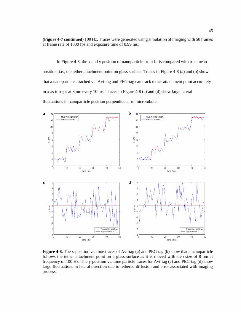
45

(Figure 4-7 continued) 100 Hz. Traces were generated using simulation of imaging with 50 frames

at frame rate of 1000 fps and exposure time of 0.99 ms.

In Figure 4-8, the x and y position of nanoparticle from fit is compared with true mean

position, i.e., the tether attachment point on glass surface. Traces in Figure 4-8 (a) and (b) show

that a nanoparticle attached via Avi-tag and PEG-tag can track tether attachment point accurately

in x as it steps at 8 nm every 10 ms. Traces in Figure 4-8 (c) and (d) show large lateral

fluctuations in nanoparticle position perpendicular to microtubule.

Figure 4-8. The x-position vs. time traces of Avi-tag (a) and PEG-tag (b) show that a nanoparticle

follows the tether attachment point on a glass surface as it is moved with step size of 8 nm at

frequency of 100 Hz. The y-position vs. time particle traces for Avi-tag (c) and PEG-tag (d) show

large fluctuations in lateral direction due to tethered diffusion and error associated with imaging

process.

a b

c d

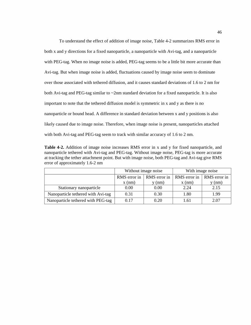
46

To understand the effect of addition of image noise, Table 4-2 summarizes RMS error in

both x and y directions for a fixed nanoparticle, a nanoparticle with Avi-tag, and a nanoparticle

with PEG-tag. When no image noise is added, PEG-tag seems to be a little bit more accurate than

Avi-tag. But when image noise is added, fluctuations caused by image noise seem to dominate

over those associated with tethered diffusion, and it causes standard deviations of 1.6 to 2 nm for

both Avi-tag and PEG-tag similar to ~2nm standard deviation for a fixed nanoparticle. It is also

important to note that the tethered diffusion model is symmetric in x and y as there is no

nanoparticle or bound head. A difference in standard deviation between x and y positions is also

likely caused due to image noise. Therefore, when image noise is present, nanoparticles attached

with both Avi-tag and PEG-tag seem to track with similar accuracy of 1.6 to 2 nm.

Table 4-2. Addition of image noise increases RMS error in x and y for fixed nanoparticle, and

nanoparticle tethered with Avi-tag and PEG-tag. Without image noise, PEG-tag is more accurate

at tracking the tether attachment point. But with image noise, both PEG-tag and Avi-tag give RMS

error of approximately 1.6-2 nm

Without image noise With image noise

RMS error in

x (nm)

RMS error in

y (nm)

RMS error in

x (nm)

RMS error in

y (nm)

Stationary nanoparticle 0.00 0.00 2.24 2.15

Nanoparticle tethered with Avi-tag 0.31 0.30 1.80 1.99

Nanoparticle tethered with PEG-tag 0.17 0.20 1.61 2.07

47

Chapter 5

Conclusions and Future Directions

Computational modelling based on reasonable assumptions and experimental constraints

can be used to characterize nanoscale motion of kinesin-1 head position with and without

nanoparticle. The three-dimensional simulation shows that in addition to Brownian diffusion and

the force of a thermodynamic spring in the neck-linker and the tethers attached to the head,

collisions of the head and the nanoparticle along with the three-dimensional geometry, especially

microtubule geometry plays a key role in determining the dynamics. In addition, it was found that

in the two head bound state although motion of a nanoparticle attached via Avi-tag is skewed to

the right side of microtubule, Avi-tag is more accurate in tracking the kinesin-1 head along the

microtubule than PEG-tag. In one head bound case, Avi-tag and PEG-tag tracked kinesin-1 head

with similar accuracy. Moreover, not much difference was observed between the effect of Avi-tag

and PEG-tag on overall head position distribution, but PEG-tag produced significantly larger

forces in neck-linkers than Avi-tag. Therefore, effect of the attached tether on the position of a

target molecule as well as on forces experienced by a target molecular should be carefully

considered for selecting an appropriate tether for tracking experiments.

From imaging simulations without any added noise, it was discovered that the effect of

particle size has drastic effect on RMS error. Contour length also had significant effect on RMS

error. Persistence length on the other hand has very little effect on RMS error. Therefore, particle

size and contour length of the tether are important parameters to consider to minimize error

associated with tethered diffusion of nanoparticle.

48

The effect of Avi-tag vs. PEG-tag can be studied further by making simulated movies of

Kinesin stepping at some frequency where particle dynamics simulation data for different states

such as one head bound and two head bound states could be used to make simulated movies by

adding image noise. This data can be compared with experimental results to further validate this

model.

In conclusion, three-dimensional geometry as well as particle size and mechanical

parameters are important to track a target accurately without perturbing the natural system

significantly. Computational modelling can be used as a tool to decide various experimental

parameters such as particle size and type of tether best suited for the application.

49

REFERENCES

[1] C. J. Lawrence, “A standardized kinesin nomenclature,” J. Cell Biol., vol. 167, no. 1, pp.

19–22, 2004.

[2] R. D. Vale, T. S. Reese, and M. P. Sheetz, “Identification of a novel force-generating

protein, kinesin, involved in microtubule-based motility,” Cell, vol. 42, no. 1, pp. 39–50,

1985.

[3] W. O. Hancock, “Bidirectional cargo transport: moving beyond tug of war,” Nat. Rev.

Mol. Cell Biol., vol. 15, no. 9, pp. 615–628, 2014.

[4] E. Chevalier-Larsen and E. L. Holzbaur, “Axonal transport and neurodegenerative

disease,” Biochim. Biophys. Acta, vol. 1762, no. 11–12, pp. 1094–1108, 2006.

[5] L. G. Bilsland, E. Sahai, G. Kelly, M. Golding, L. Greensmith, and G. Schiavo, “Deficits

in axonal transport precede ALS symptoms in vivo.,” Proc. Natl. Acad. Sci. U. S. A., vol.

107, no. 47, pp. 20523–20528, 2010.

[6] G. a Morfini et al., “Pathogenic huntingtin inhibits fast axonal transport by activating

JNK3 and phosphorylating kinesin.,” Nat. Neurosci., vol. 12, no. 7, pp. 864–871, 2009.

[7] A.-L. Ström, J. Gal, P. Shi, E. J. Kasarskis, L. J. Hayward, and H. Zhu, “Retrograde

axonal transport and motor neuron disease.,” J. Neurochem., vol. 106, no. 2, pp. 495–505,

2008.

[8] E. Perlson et al., “A Switch in Retrograde Signaling from Survival to Stress in Rapid-

Onset Neurodegeneration,” J. Neurosci., vol. 29, no. 31, pp. 9903–9917, 2009.

50

[9] Y. Chen, M. M. Rolls, and W. O. Hancock, “An EB1-Kinesin Complex Is Sufficient to

Steer Microtubule Growth In Vitro,” Curr. Biol., vol. 24, no. 3, pp. 316–321, 2014.

[10] V. Mennella, G. C. Rogers, S. L. Rogers, D. W. Buster, R. D. Vale, and D. J. Sharp,

“Functionally distinct kinesin-13 family members cooperate to regulate microtubule

dynamics during interphase,” Nat Cell Biol, vol. 7, no. 3, pp. 235–245, 2005.

[11] A. M. Saunders, J. Powers, S. Strome, and W. M. Saxton, “Kinesin-5 acts as a brake in

anaphase spindle elongation,” Curr. Biol., vol. 17, no. 12, pp. 453–454, 2007.

[12] G. Bergnes, K. Brejc, and L. Belmont, “Mitotic Kinesins: Prospects for Antimitotic Drug

Discovery,” Curr. Top. Med. Chem., vol. 5, no. 2, pp. 127–145, 2005.

[13] C. L. Asbury, A. N. Fehr, and S. M. Block, “Kinesin moves by an asymmetric hand-over-

hand mechanism.,” Science, vol. 302, no. 5653, pp. 2130–4, 2003.

[14] S. Rice et al., “A structural change in the kinesin motor protein that drives motility.,”

Nature, vol. 402, no. 6763, pp. 778–84, 1999.

[15] M. L. Kutys, J. Fricks, and W. O. Hancock, “Monte Carlo analysis of neck linker

extension in kinesin molecular motors.,” PLoS Comput. Biol., vol. 6, no. 11, p. e1000980,

2010.

[16] K. J. Mickolajczyk, N. C. Deffenbaugh, J. Ortega Arroyo, J. Andrecka, P. Kukura, and W.

O. Hancock, “Kinetics of nucleotide-dependent structural transitions in the kinesin-1

hydrolysis cycle.,” Proc. Natl. Acad. Sci. U. S. A., vol. 112, no. 52, pp. E7186-93, 2015.

[17] H. Isojima, R. Iino, Y. Niitani, H. Noji, and M. Tomishige, “Direct observation of

intermediate states during the stepping motion of kinesin-1,” Nat. Chem. Biol., vol. 12, no.

4, pp. 290–297, 2016.

[18] F. Ruhnow, D. Zwicker, and S. Diez, “Tracking single particles and elongated filaments

51

with nanometer precision,” Biophys. J., vol. 100, no. 11, pp. 2820–2828, 2011.

[19] A. N. Fehr, C. L. Asbury, and S. M. Block, “Kinesin steps do not alternate in size.,”

Biophys. J., vol. 94, no. 3, pp. L20-2, 2008.

[20] E. P. Sablin, F. J. Kull, R. Cooke, R. D. Vale, and R. J. Fletterick, “Crystal structure of the

motor domain of the kinesin-related motor ncd.,” Nature, vol. 380, no. 6574. pp. 555–9,

1996.

[21] G. J. Hoeprich, A. R. Thompson, D. P. McVicker, W. O. Hancock, and C. L. Berger,

“Kinesin’s Neck-Linker Determines its Ability to Navigate Obstacles on the Microtubule

Surface,” Biophys. J., vol. 106, no. 8, pp. 2–8, 2014.

[22] W. Hwang, M. J. Lang, and M. Karplus, “Force Generation in Kinesin Hinges on Cover-

Neck Bundle Formation,” Structure, vol. 16, no. 1, pp. 62–71, 2008.

[23] H. Lee, R. M. Venable, A. D. Mackerell, and R. W. Pastor, “Molecular dynamics studies

of polyethylene oxide and polyethylene glycol: hydrodynamic radius and shape

anisotropy.,” Biophys. J., vol. 95, no. 4, pp. 1590–9, 2008.

[24] Thermo Fisher Scientific, “21901BID: EZ-Link Maleimide-PEG2 -Biotin.”

[25] J. Kerssemakers, J. Howard, H. Hess, and S. Diez, “The distance that kinesin-1 holds its

cargo from the microtubule surface measured by fluorescence interference contrast

microscopy.,” Proc. Natl. Acad. Sci. U. S. A., vol. 103, no. 43, pp. 15812–15817, 2006.

[26] P. C. Nelson, C. Zurla, D. Brogioli, J. F. Beausang, L. Finzi, and D. Dunlap, “Tethered

particle motion as a diagnostic of DNA tether length,” J. Phys. Chem. B, vol. 110, no. 34,

pp. 17260–17267, 2006.

[27] V. Hariharan and W. O. Hancock, “Insights into the Mechanical Properties of the Kinesin

Neck Linker Domain from Sequence Analysis and Molecular Dynamics Simulations,”

52

Cell Mol Bioeng., vol. 2, no. 2, pp. 177–189, 2009.

[28] D. E. Segall, P. C. Nelson, and R. Phillips, “Volume-exclusion effects in tethered-particle

experiments: Bead size matters,” Phys. Rev. Lett., vol. 96, no. 8, pp. 1–4, 2006.

[29] F. N. Hooge and A. M. H. Hoppenbrouwers, “Amplitude distribution of Shot Noise,”

Physica, vol. 42, no. l, pp. 331–339, 1969.

53

Appendix A

MATLAB Code for Worm-like Chain Force Calculation

function [f_s] = f_WLC(T,Lp,Lc,x,x0,max_f) %Inputs: T = Temperature in K, Lp = Persistence Length of chain, Lc = %Contour Length of Chain, x = end-to-end distance of chain, freeheadpos = %position of free head, x0 is equilibrium position where spring force is %zero %Outputs: f_s = spring force generated by Worm-Like Chain k_B = 1.3806488e-2; %Boltzmann's constant (in pN*nm/K) if x >= x0 x = x - x0; f = k_B*T/Lp*(1/4*(1-x/Lc).^(-2) - 1/4 + x/Lc); else x = -(x - x0); f = -k_B*T/Lp*(1/4*(1-x/Lc).^(-2) - 1/4 + x/Lc); end if abs(f) >= max_f f_s = sign(f)*max_f; else f_s = f; end

54

Appendix B

MATLAB Code for Particle Dynamics Simulation for Single Molecule Experiment for One

Head Bound Case with Undocked Neck-linker and Nanoparticle attached with Avi-tag

%Particle dynamics simulation for single molecule experiments %One head bound case with undocked neck-linked %Nanoparticle is attached with Avi-tag %Note: coordinate system used for calculation is different from that %used to report results (y_calc = z_result, z_calc = -y_result) clear all close all clc %Input Parameters N_tot = 1; %Total number of .mat files n = 1e6; %Number of points in each .mat file dt = 1e-9; %Simulation time step %Physical input parameters r_np = 15; %radius of nanoparticle (nm) r_h = 2.5; %radius of kinesin head (nm) r_MT = 12.5; %radius of microtubule (nm) eta = 8.9e-10; %dynamic viscocity of water at 25 C (pN*s/nm^2) f_h = 6*pi*eta*r_h; %viscous drag coefficient for kinesin head(pN*s/nm) f_np = 6*pi*eta*r_np; %viscouns drag coefficient for nanoparticle (pN*s/nm) T_C = 25; %temperature (C) T_K = T_C + 273.15; %temperature (K) k_B = 1.3806488e-2; %Boltzmann's constant (pN*nm/K) D_h = k_B*T_K/f_h; %coefficient of diffusion (nm^2/s) D_np = k_B*T_K/f_np; %coefficient of diffusion (nm^2/s) %Tether attachment point coh2coNL = r_h; %distance from center of head to center of neck-linker; if tether is sticking out of right

side of head, it will be r_h coh2coAvi = 0; %distance from center of head to center of Avi-tag; if tether is sticking out of right side of

head (two head bound case), it will be r_h %Contour length Lc_AA = 0.38; %Contour length of each amino acid (nm) AA_NL = 14; %Number of amino acids in neck-linker AA_CS = 13; %Number of amino acids in cover strand AA_Avi = 14 + 3; %Number of amino acids in Avi-tag

55

Lc_dNL = AA_NL*Lc_AA; %Contour length of docked neck-linker (nm) Lc_uNL = 2*AA_NL*Lc_AA; %Contour length of undocked neck-linkers (nm) Lc_Avi = (AA_Avi + AA_CS)*Lc_AA; %Contour length of Avi-tag (nm) Lc_PEG = 2.91; %Contour length of PEG-tag (nm) %Persistence length Lp_Avi = 1; %Persistence length of Avi-tag (nm) Lp_PEG = 0.38; %Persistence length of PEG-tag (nm) Lp_NL = 1; %Persistence length of neck-linkers (nm) %Offset in head and NP position due to docking of NL x0_h = 0; %displacement of mean position of head. If NL is undocked, x0_h = 0; If NL is docked, x0_h =

Lc_dNL x0_np = 0; %displacement of mean position of nanoparticle min_dist_h_h = r_h; %Minimum distance between center of unbound head and neck-linker attachment

point on bound head surface min_dist_h_np = r_h + r_np; %Minimum distance between center of nanoparticle and Avi-tag attachment

point ( %Assign persistence and contour lengths Lc_Avi = Lc_Avi; %Contour length of Avi-tag (nm). For Avi-tag use Lc_Avi. For PEG-tag use Lc_PEG Lp_Avi = Lp_Avi; %Persistence length of Avi-tag (nm). For Avi-tag use Lp_Avi. For PEG-tag use

Lp_PEG Lp_NL = Lp_NL; %Persistence length of NL (nm) Lc_NL = Lc_uNL; %Contour length of NL (nm) %First initial condition bhx = 0; bhy = r_h; bhz = 0; uhx_ini = bhx(1) + x0_h; uhy_ini = bhy(1) + min_dist_h_h + 0.5*Lc_NL; uhz_ini = bhz(1) + coh2coNL; npx_ini = uhx_ini + x0_np; npy_ini = uhy_ini + min_dist_h_np + 0.5*Lc_Avi; npz_ini = uhz_ini + coh2coAvi; for N = 1:N_tot %for each .mat file %Initialization uhx = zeros(1,n+1); uhy = zeros(1,n+1); uhz = zeros(1,n+1); npx = zeros(1,n+1); npy = zeros(1,n+1); npz = zeros(1,n+1); force_h = zeros(1,n+1); force_np = zeros(1,n+1); theta_np_MT = []; L_np_MT = []; L_fAvi = zeros(1,n+1); L_fNL = zeros(1,n+1);

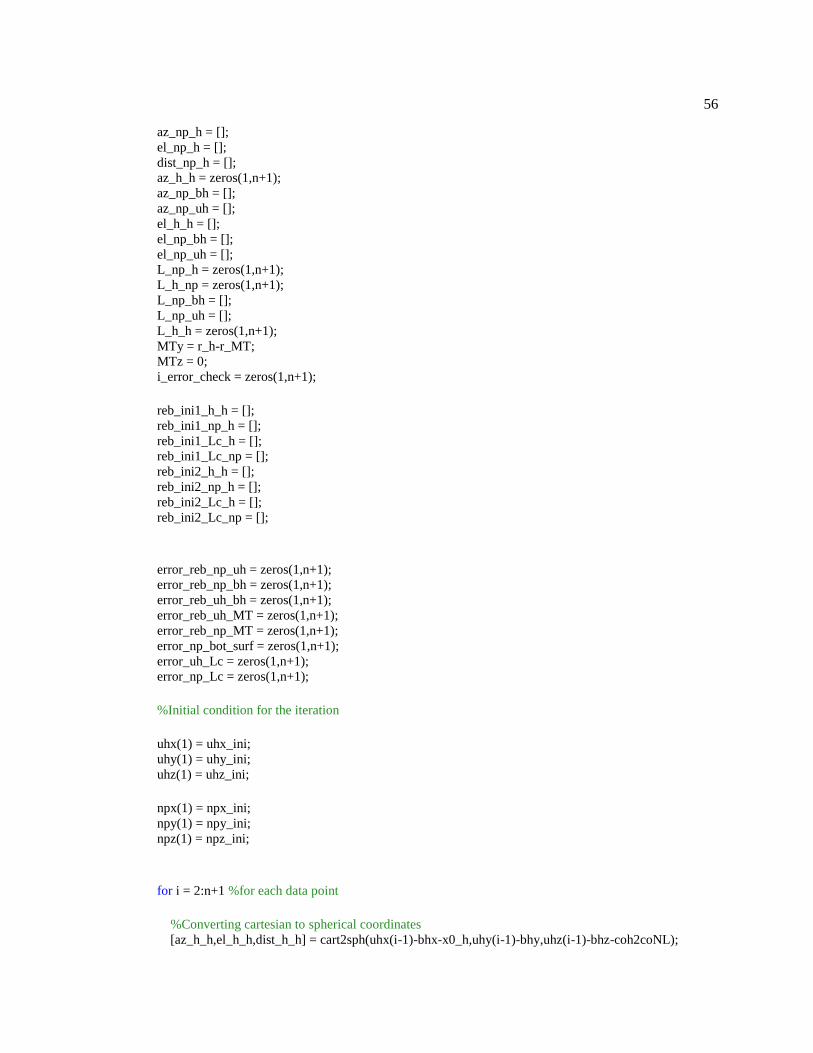
56

az_np_h = []; el_np_h = []; dist_np_h = []; az_h_h = zeros(1,n+1); az_np_bh = []; az_np_uh = []; el_h_h = []; el_np_bh = []; el_np_uh = []; L_np_h = zeros(1,n+1); L_h_np = zeros(1,n+1); L_np_bh = []; L_np_uh = []; L_h_h = zeros(1,n+1); MTy = r_h-r_MT; MTz = 0; i_error_check = zeros(1,n+1); reb_ini1_h_h = []; reb_ini1_np_h = []; reb_ini1_Lc_h = []; reb_ini1_Lc_np = []; reb_ini2_h_h = []; reb_ini2_np_h = []; reb_ini2_Lc_h = []; reb_ini2_Lc_np = [];

error_reb_np_uh = zeros(1,n+1); error_reb_np_bh = zeros(1,n+1); error_reb_uh_bh = zeros(1,n+1); error_reb_uh_MT = zeros(1,n+1); error_reb_np_MT = zeros(1,n+1); error_np_bot_surf = zeros(1,n+1); error_uh_Lc = zeros(1,n+1); error_np_Lc = zeros(1,n+1); %Initial condition for the iteration uhx(1) = uhx_ini; uhy(1) = uhy_ini; uhz(1) = uhz_ini; npx(1) = npx_ini; npy(1) = npy_ini; npz(1) = npz_ini;

for i = 2:n+1 %for each data point %Converting cartesian to spherical coordinates [az_h_h,el_h_h,dist_h_h] = cart2sph(uhx(i-1)-bhx-x0_h,uhy(i-1)-bhy,uhz(i-1)-bhz-coh2coNL);

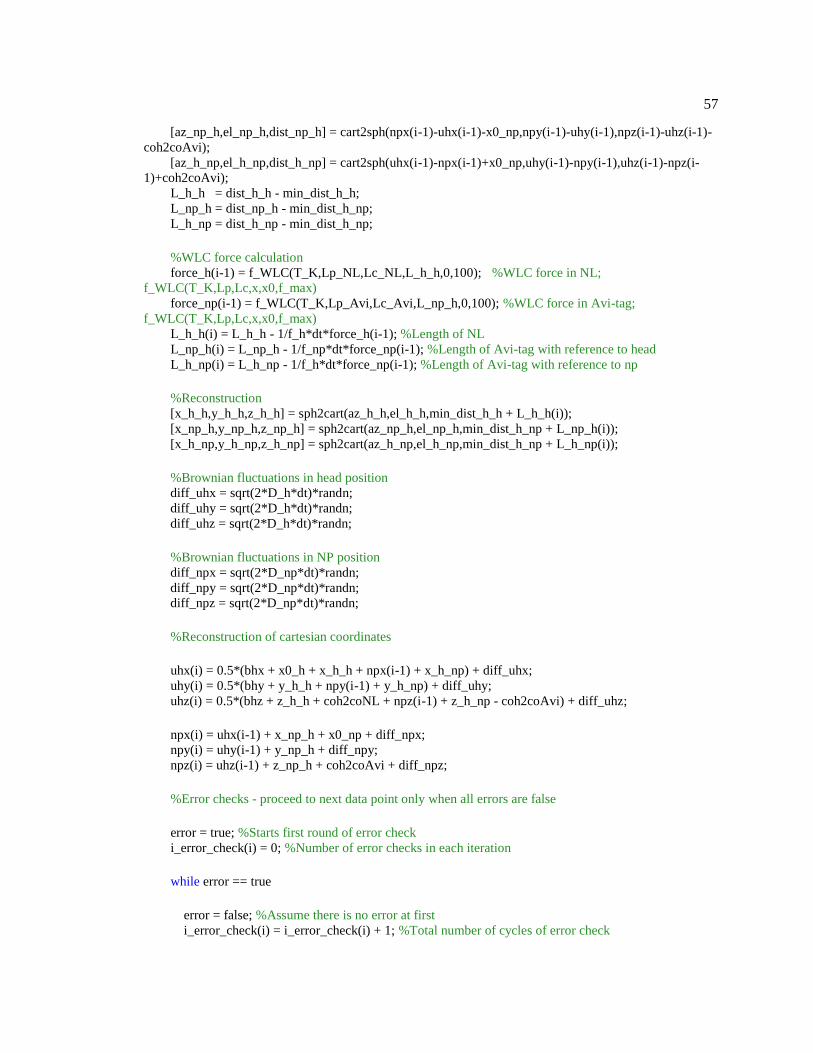
57

[az_np_h,el_np_h,dist_np_h] = cart2sph(npx(i-1)-uhx(i-1)-x0_np,npy(i-1)-uhy(i-1),npz(i-1)-uhz(i-1)-

coh2coAvi); [az_h_np,el_h_np,dist_h_np] = cart2sph(uhx(i-1)-npx(i-1)+x0_np,uhy(i-1)-npy(i-1),uhz(i-1)-npz(i-

1)+coh2coAvi); L_h_h = dist_h_h - min_dist_h_h; L_np_h = dist_np_h - min_dist_h_np; L_h_np = dist_h_np - min_dist_h_np; %WLC force calculation force_h(i-1) = f_WLC(T_K,Lp_NL,Lc_NL,L_h_h,0,100); %WLC force in NL;

f_WLC(T_K,Lp,Lc,x,x0,f_max) force_np(i-1) = f_WLC(T_K,Lp_Avi,Lc_Avi,L_np_h,0,100); %WLC force in Avi-tag;

f_WLC(T_K,Lp,Lc,x,x0,f_max) L_h_h(i) = L_h_h - 1/f_h*dt*force_h(i-1); %Length of NL L_np_h(i) = L_np_h - 1/f_np*dt*force_np(i-1); %Length of Avi-tag with reference to head L_h_np(i) = L_h_np - 1/f_h*dt*force_np(i-1); %Length of Avi-tag with reference to np %Reconstruction [x_h_h,y_h_h,z_h_h] = sph2cart(az_h_h,el_h_h,min_dist_h_h + L_h_h(i)); [x_np_h,y_np_h,z_np_h] = sph2cart(az_np_h,el_np_h,min_dist_h_np + L_np_h(i)); [x_h_np,y_h_np,z_h_np] = sph2cart(az_h_np,el_h_np,min_dist_h_np + L_h_np(i)); %Brownian fluctuations in head position diff_uhx = sqrt(2*D_h*dt)*randn; diff_uhy = sqrt(2*D_h*dt)*randn; diff_uhz = sqrt(2*D_h*dt)*randn; %Brownian fluctuations in NP position diff_npx = sqrt(2*D_np*dt)*randn; diff_npy = sqrt(2*D_np*dt)*randn; diff_npz = sqrt(2*D_np*dt)*randn; %Reconstruction of cartesian coordinates uhx(i) = 0.5*(bhx + x0_h + x_h_h + npx(i-1) + x_h_np) + diff_uhx; uhy(i) = 0.5*(bhy + y_h_h + npy(i-1) + y_h_np) + diff_uhy; uhz(i) = 0.5*(bhz + z_h_h + coh2coNL + npz(i-1) + z_h_np - coh2coAvi) + diff_uhz; npx(i) = uhx(i-1) + x_np_h + x0_np + diff_npx; npy(i) = uhy(i-1) + y_np_h + diff_npy; npz(i) = uhz(i-1) + z_np_h + coh2coAvi + diff_npz; %Error checks - proceed to next data point only when all errors are false error = true; %Starts first round of error check i_error_check(i) = 0; %Number of error checks in each iteration while error == true error = false; %Assume there is no error at first i_error_check(i) = i_error_check(i) + 1; %Total number of cycles of error check

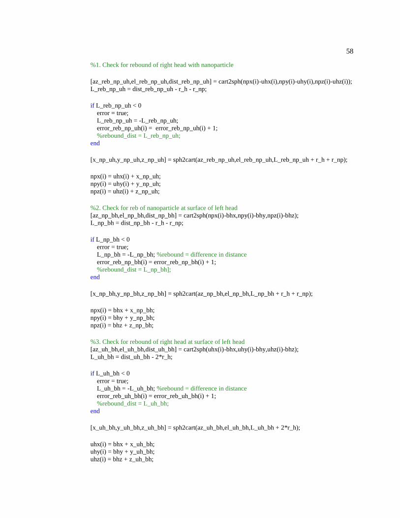
58

%1. Check for rebound of right head with nanoparticle [az_reb_np_uh,el_reb_np_uh,dist_reb_np_uh] = cart2sph(npx(i)-uhx(i),npy(i)-uhy(i),npz(i)-uhz(i)); L_reb_np_uh = dist_reb_np_uh - r_h - r_np; if L_reb_np_uh < 0 error = true; L_reb_np_uh = -L_reb_np_uh; error_reb_np_uh(i) = error_reb_np_uh(i) + 1; %rebound_dist = L_reb_np_uh; end [x_np_uh,y_np_uh,z_np_uh] = sph2cart(az_reb_np_uh,el_reb_np_uh,L_reb_np_uh + r_h + r_np); npx(i) = uhx(i) + x_np_uh; npy(i) = uhy(i) + y_np_uh; npz(i) = uhz(i) + z_np_uh; %2. Check for reb of nanoparticle at surface of left head [az_np_bh,el_np_bh,dist_np_bh] = cart2sph(npx(i)-bhx,npy(i)-bhy,npz(i)-bhz); L_np_bh = dist_np_bh - r_h - r_np; if L_np_bh < 0 error = true; L_np_bh = -L_np_bh; %rebound = difference in distance error_reb_np_bh(i) = error_reb_np_bh(i) + 1; %rebound_dist = L_np_bh]; end [x_np_bh,y_np_bh,z_np_bh] = sph2cart(az_np_bh,el_np_bh,L_np_bh + r_h + r_np); npx(i) = bhx + x_np_bh; npy(i) = bhy + y_np_bh; npz(i) = bhz + z_np_bh; %3. Check for rebound of right head at surface of left head [az_uh_bh,el_uh_bh,dist_uh_bh] = cart2sph(uhx(i)-bhx,uhy(i)-bhy,uhz(i)-bhz); L_uh_bh = dist_uh_bh - 2*r_h; if L_uh_bh < 0 error = true; L_uh_bh = -L_uh_bh; %rebound = difference in distance error_reb_uh_bh(i) = error_reb_uh_bh(i) + 1; %rebound_dist = L_uh_bh; end [x_uh_bh,y_uh_bh,z_uh_bh] = sph2cart(az_uh_bh,el_uh_bh,L_uh_bh + 2*r_h); uhx(i) = bhx + x_uh_bh; uhy(i) = bhy + y_uh_bh; uhz(i) = bhz + z_uh_bh;

59

%4. Check for rebound of right head at MT [theta_uh_MT,dist_uh_MT] = cart2pol(uhz(i)-MTz,uhy(i)-MTy); L_uh_MT = dist_uh_MT - r_MT - r_h; if L_uh_MT < 0 error = true; L_uh_MT = -L_uh_MT; error_reb_uh_MT(i) = error_reb_uh_MT(i) + 1; %rebound_dist = L_uh_MT; end [z_uh_MT,y_uh_MT] = pol2cart(theta_uh_MT,L_uh_MT + r_MT + r_h); uhz(i) = MTz + z_uh_MT; uhy(i) = MTy + y_uh_MT; %5. Check for rebound of nanoparticle at MT [theta_np_MT,dist_np_MT] = cart2pol(npz(i)-MTz,npy(i)-MTy); L_np_MT = dist_np_MT - r_MT - r_np; if L_np_MT < 0 error = true; L_np_MT = -L_np_MT; error_reb_np_MT(i) = error_reb_np_MT(i) + 1; %rebound_dist = L_np_MT; end [z_np_MT,y_np_MT] = pol2cart(theta_np_MT,L_np_MT + r_MT + r_np); npz(i) = MTz + z_np_MT; npy(i) = MTy + y_np_MT; %6. Check for rebound of nanoparticle at bottom surface if npy(i) - r_np < -r_h - 2*r_MT error = true; npy(i) = r_np - r_h - 2*r_MT - (npy(i) - r_np + r_h + 2*r_MT); error_np_bot_surf(i) = error_np_bot_surf(i) + 1; %rebound_dist = npy(i) - r_np + r_h + 2*r_MT; end %7. Check for rebound of right head at contour length [az_uh_bh,el_uh_bh,dist_uh_bh] = cart2sph(uhx(i)-bhx-x0_h,uhy(i)-bhy,uhz(i)-bhz-coh2coNL); L_fNL(i) = dist_uh_bh - min_dist_h_h; if L_fNL(i) > Lc_NL error = true; L_fNL(i) = Lc_NL - (L_fNL(i) - Lc_NL); error_uh_Lc(i) = error_uh_Lc(i) + 1; %rebound_dist = Lc_NL - L_fNL(i); end

60

[x_uh_bh_Lc,y_uh_bh_Lc,z_uh_bh_Lc] = sph2cart(az_uh_bh,el_uh_bh,min_dist_h_h + L_fNL(i)); uhx(i) = bhx + x_uh_bh_Lc + x0_h; uhy(i) = bhy + y_uh_bh_Lc; uhz(i) = bhz + z_uh_bh_Lc + coh2coNL; %8. Check for rebound of nanoparticle at contour length [az_np_uh,el_np_uh,dist_np_uh] = cart2sph(npx(i)-uhx(i)-x0_np,npy(i)-uhy(i),npz(i)-uhz(i)-

coh2coAvi); L_fAvi(i) = dist_np_uh - min_dist_h_np; if L_fAvi(i) > Lc_Avi error = true; L_fAvi(i) = Lc_Avi - (L_fAvi(i) - Lc_Avi); error_np_Lc(i) = error_np_Lc(i) + 1; %rebound_dist = Lc_Avi - L_fAvi; end [x_np_uh_Lc,y_np_uh_Lc,z_np_uh_Lc] = sph2cart(az_np_uh,el_np_uh,min_dist_h_np +

L_fAvi(i)); npx(i) = uhx(i) + x_np_uh_Lc + x0_np; npy(i) = uhy(i) + y_np_uh_Lc; npz(i) = uhz(i) + z_np_uh_Lc + coh2coAvi; end end %Exchange y and z axes (because axes used for calculation and %axes used for results are different) npZ = npy; npy = -npz; npz = npZ; clear npZ uhZ = uhy; uhy = -uhz; uhz = uhZ; clear uhZ bhZ = bhy; bhy = -bhz; bhz = bhZ; clear bhZ %Reassign initial values for next iteration of N (Note change in %coodinate system mentioned above) uhx_ini = uhx(end);

61

uhy_ini = uhz(end); uhz_ini = -uhy(end); npx_ini = npx(end); npy_ini = npz(end); npz_ini = -npy(end); end

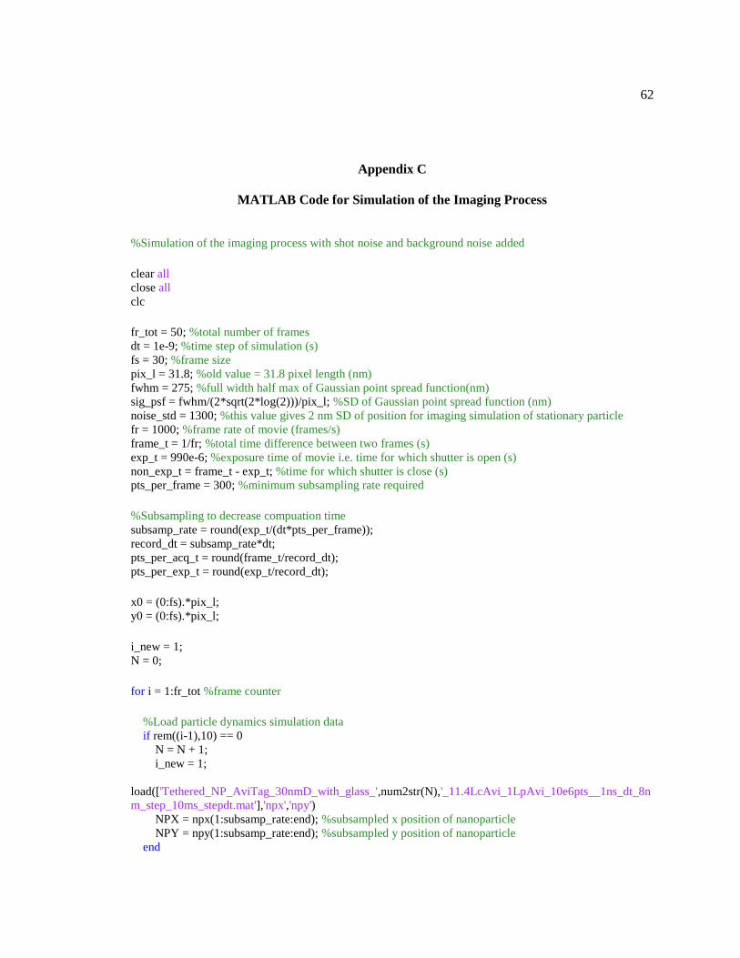
62

Appendix C

MATLAB Code for Simulation of the Imaging Process

%Simulation of the imaging process with shot noise and background noise added clear all close all clc fr_tot = 50; %total number of frames dt = 1e-9; %time step of simulation (s) fs = 30; %frame size pix_l = 31.8; %old value = 31.8 pixel length (nm) fwhm = 275; %full width half max of Gaussian point spread function(nm) sig_psf = fwhm/(2*sqrt(2*log(2)))/pix_l; %SD of Gaussian point spread function (nm) noise_std = 1300; %this value gives 2 nm SD of position for imaging simulation of stationary particle fr = 1000; %frame rate of movie (frames/s) frame_t = 1/fr; %total time difference between two frames (s) exp_t = 990e-6; %exposure time of movie i.e. time for which shutter is open (s) non_exp_t = frame_t - exp_t; %time for which shutter is close (s) pts_per_frame = 300; %minimum subsampling rate required %Subsampling to decrease compuation time subsamp_rate = round(exp_t/(dt*pts_per_frame)); record_dt = subsamp_rate*dt; pts_per_acq_t = round(frame_t/record_dt); pts_per_exp_t = round(exp_t/record_dt); x0 = (0:fs).*pix_l; y0 = (0:fs).*pix_l; i_new = 1; N = 0; for i = 1:fr_tot %frame counter %Load particle dynamics simulation data if rem((i-1),10) == 0 N = N + 1; i_new = 1;

load(['Tethered_NP_AviTag_30nmD_with_glass_',num2str(N),'_11.4LcAvi_1LpAvi_10e6pts__1ns_dt_8n

m_step_10ms_stepdt.mat'],'npx','npy') NPX = npx(1:subsamp_rate:end); %subsampled x position of nanoparticle NPY = npy(1:subsamp_rate:end); %subsampled y position of nanoparticle end

63

i = i_new; image = zeros(fs); for ii = (i-1)*pts_per_acq_t+1:(i-1)*pts_per_acq_t+pts_per_exp_t %for each subsampled position visible

to camera during exposure time of the frame xc = pix_l*15.5 + NPX(ii); yc = pix_l*15.5 + NPY(ii); x = (x0-xc)/pix_l; y = (y0-fs*pix_l+yc)/pix_l; for r = 1:fs for c = 1:fs image(r,c) = image(r,c) + 1/pix_l^2*cdf_int(x(c),y(r),x(c+1),y(r+1),0,sig_psf); %add pixel values

for 2D Gassian corresponding to each visible position end end end image = flipud(image); image = 0.25*image/(max(max(image))); %scale by 1/4 to ensure no oversaturation of the frame im = round(image*65535); %convert to 16-bit values im = poissrnd(im) + normrnd(0,noise_std,size(im)); %add shot noise (Poisson noise) and background

noise (Gaussian noise) im = uint16(im);

imwrite(im,['Movie_Tethered_NP_AviTag_with_noise_',num2str(pts_per_frame),'ptsperframe_',num2str(f

r),'fps_',num2str(exp_t*1e6),'us_exp_t.tif'],'Compression','None','WriteMode','append') i_new = i_new + 1; end

64

ACADEMIC VITA

Janak P. Jethva

[email protected]

________________________________________

Education

B.S., Biomedical Engineering, 2017, The Pennsylvania State University, University Park, PA

M.S., Biomedical Engineering, 2017, The Pennsylvania State University, University Park, PA

Honors and Awards

Penn State Student Leader Scholarship December, 2016

Global Challenge Scholar, National Academy of Engineering April, 2016

Fresenius Medical Care Scholarship August, 2015

John Deere Scholarship September, 2015

Humanitarian Engineering and Social Entrepreneurship Change Agent Award May, 2015

Second Place in Penn State Hazleton Mathematics Olympiad May, 2014

The President’s Freshman Award May, 2014

The President Sparks Award August, 2014

Schreyer Honors Scholar, Schreyer Honors College August, 2012

Association Memberships/Activities

• Biomedical Engineering Society

• Tau Beta Pi (Engineering Honor Society)

• Association for India’s Development

• Society for Indian Music and Arts

65

Professional Experience

Research Assistant (May 2014 – Present)

Biomedical Engineering Department, The Pennsylvania State University, University Park, PA

Modelled and simulated the nanoscale motion of Kinesin motor protein using MATLAB

programming language, which is important to understand for better treatment of cancer

and neurodegenerative diseases

Experienced with site-directed mutagenesis with E. Coli cell line, Polymerase Chain

Reaction (PCR), optical microscopy, total internal reflection fluorescence (TIRF)

microscopy, and in vitro motility assays

Provided figures and data for a successful NIH R01 grant proposal

Presented research in Biomedical Engineering Society Annual Meeting 2016

Grader (August 2016 – December 2016)

The Pennsylvania State University, University Park, PA

Graded homework assignments for biomedical engineering course focused on modelling

of physiological systems as linear systems

Provided one-on-one tutoring for the course

Project Developer (January 2015 – August 2015)

Humanitarian Engineering and Social Entrepreneurship (HESE) Program, The Pennsylvania State

University, University Park, PA

Designed and tested a novel manufacturing method of using inkjet printers to produce low-

cost urinary test strips to detect diabetes and urinary tract infections for people in Africa

Conducted fieldwork in Zambia during summer 2015 by studying current diagnostic

pathways for these diseases and market channels for the test strips

66

Strategized comprehensive business model for this venture which has won more than

$25,000 in grants

Presented research in three international humanitarian engineering conferences

Co-authored a paper in Journal of Medical Engineering & Technology and an IEEE GHTC

conference article

Member of Photonics Research Group (January 2013 – December 2013)

Photonics Lab, The Pennsylvania State University, Hazleton, PA

Worked under Physics professor Dr. David Starling along with select other students to do

research in building single photon detector

In first semester, a photon intensity detector was made using avalanche photo-diode and

operational-amplifier

In second semester, an active-quenching circuit was designed to reset the bias voltage

applied on avalanche photo-diode using bipolar junction transistor

Mathematics Tutor (September, 2012 – December 2013)

Math Dimensions, The Pennsylvania State University, Hazleton, PA

Tutored students in various mathematics courses from algebra through differential

equations

Held class review sessions for multi-variable calculus and linear algebra

Held one-on-one tutoring sessions for statistics

Professional Presentations

“Modelling Nanoscale Dynamics of Molecular Motors”, Biomedical Engineering Society

Annual Meeting 2016

“Can We Manufacture Diagnostic Test Strips Using an Inkjet Printer?”, IEEE Global

Humanitarian Technology Conference 2015, Seattle, WA

67

“Ukweli Test Strips”, VentureWell Open 2015 Conference, Washington, DC

“I dream of a Product Characterization Lab”, VentureWell Open 2016 Conference,

Portland, OR

“3D Simulation of Gold Nanoparticle Tracking of Kinesin-1”, The Summer Translational

Cardiovascular Science Institute, The Pennsylvania State University, University Park, PA

“Monte Carlo Simulation of Gold Nanoparticle Tracking of Kinesin-1”. Penn

State College of Engineering. Research Experience for Undergraduates, The

Pennsylvania State University, University Park, PA

Publications and Papers

Frazzette, N., Dobson, J., Mukhtar, A., Burt, B., Jethva, J., Adair, J., & Mehta, K. (2015).

Can we manufacture diagnostic test strips using an Inkjet printer? 2015 IEEE Global

Humanitarian Technology Conference (GHTC). doi:10.1109/ghtc.2015.7344008

Frazzette, N., Jethva, J., Mehta, K., Stapleton, J. J., & Randall, C. (2016). Designing a

ruggedisation lab to characterise materials for harsh environments. Journal of Medical

Engineering & Technology,40(7-8), 383-391. doi:10.1080/03091902.2016.1213905

NANO-SCALE SIMULATION OF GOLD NANOPARTICLE TRACKING …

Documents

Transcript of NANO-SCALE SIMULATION OF GOLD NANOPARTICLE TRACKING …