Name:Qiaofeng Cui Septemper 2014 Master’s Thesis in ...

FACULTY OF ENGINEERING AND SUSTAINABLE DEVELOPMENT .

Suppression of impulsive noise in wireless communication

Name:Qiaofeng Cui

Septemper 2014

Master’s Thesis in Electronics

Master’s Program in Electronics/Telecommunications

Examiner: Jose Chilo

Name:Qiaofeng Cui Suppression of impulsive noise in wireless communication

iii

Preface

By the time when I finish my thesis, I would like to say thank you to all the teachers and classmates

who ever helped me in the past.

Also, a special thank would be given to my personal tutor, who has been so kind to me, giving me all

the best advices. At the same time, I want to thank all the students who once worked, studied together

with me in the laboratory, the lecture room and the library.

Finally, I would like to thank myself and my parents, who had been always with me, taking cares of

me, and leading my way out from hard times.


iv


v

Abstract

This report intends to verify the possibility that the FastICA algorithm could be applied to the GPS

system to eliminate the impulsive noise from the receiver end. As the impulsive noise is so unpredictable

in its pattern and of great energy level to swallow the signal we need, traditional signal selection methods

exhibit no much use in dealing with this problem. Blind Source Separation seems to be a good way to

solve this, but most of the other BSS algorithms beside FastICA showed more or less degrees of

dependency on the pattern of the noise. In this thesis, the basic mathematic modelling of this advanced

algorithm, along with the principles of the commonly used fast independent component analysis

(fastICA) based on fixed-point algorithm are discussed. To verify that this method is useful under

industrial use environment to remove the impulsive noises from digital BPSK modulated signals, an

observation signal mixed with additive impulsive noise is generated and separated by fastICA method.

And in the last part of the thesis, the fastICA algorithm is applied to the GPS receiver modeled in the

SoftGNSS project and verified to be effective in industrial applications. The results have been analyzed.

Key Words: GPS receiver, fastICA, BPSK, Impulsive Noise, Blind Signal Separation, Independent

Component Analysis;


vi


vii

Table of contents

Preface .................................................................................................................................................... iii

Abstract ................................................................................................................................................... v

Table of contents ................................................................................................................................... vii

Figues and Tables ................................................................................................................................... ix

1 Introduction ..................................................................................................................................... 1

1.1 Background .............................................................................................................................. 1

1.2 Goal .......................................................................................................................................... 2

1.3 Outline ...................................................................................................................................... 3

2 Basic Theories ................................................................................................................................. 4

2.1 Blind Source Separation Theory .............................................................................................. 4

2.1.1 Introduction of BSS Basics .............................................................................................. 4

2.1.2 Basic BSS Methods .......................................................................................................... 5

2.1.3 Application of BSS Algorithm ......................................................................................... 5

2.2 Mathematical Models ............................................................................................................... 6

2.2.1 General Modeling of BBS Problems ................................................................................ 6

2.2.2 General Modeling of ICA Approach ................................................................................ 7

2.3 FastICA Algorithm .................................................................................................................. 7

2.3.1 Research Background Introduction .................................................................................. 7

2.3.2 Negative Entropy Maximization Estimation Method ....................................................... 8

2.3.3 A Brief Introduction of MATLAB ................................................................................. 13

2.4 BPSK Modulation in GPS ...................................................................................................... 14

3 Simulation and Results .................................................................................................................. 16

3.1 Core Steps of the FastICA Processing ................................................................................... 16

3.2 Overview Flow Chart of the FastICA Processing .................................................................. 17

3.3 Generation of Signals ............................................................................................................. 18

3.3.1 Generation of BPSK Modulated Signals ........................................................................ 18

3.3.2 Generation of Sample Signals Mixed With Impulsive Noise ......................................... 19


viii

3.4 Application of Signal Preprocessing ...................................................................................... 21

3.4.1 Centralization Processing ............................................................................................... 22

3.4.2 Whitening Processing ..................................................................................................... 22

3.5 Application of Fixed-point Iterative Calculation ................................................................... 24

3.5.1 FastICA Iteration Loop ................................................................................................... 24

3.6 Visual Plotting and Results .................................................................................................... 26

4 FastICA Application to GPS ......................................................................................................... 31

4.1 The Impact of Impulsive Noise to GPS ................................................................................. 31

4.2 Performance of The FastICA Applied GPS Receiver ............................................................ 32

5 Discussion ..................................................................................................................................... 35

6 Conclusions ................................................................................................................................... 36

References ............................................................................................................................................. 37

Appendix A ............................................................................................................................................. 1

Appendix B ............................................................................................................................................. 3


ix

Figues and Tables

Figure 1: The Basic Communication Method For GPS. ................................................................. 2

Figure 2: ICA model block diagram. ............................................................................................... 7

Figure 3: The Generation of GPS Signals At The Satellites. (From SoftGNSS Project) .............. 15

Figure 4: The Waveform of L1 GPS Signals and Its Components. (From SoftGNSS Project) .... 15

Figure 5: The Overview Flow Chart of The FastICA Application ................................................ 18

Figure 6: Typical Binary Phase Shift Keying (BPSK) Modulated Signal..................................... 19

Figure 7: The Mixed Impulsive Noise Signal. ............................................................................. 20

Figure 8: The Mixed Observation Signal. ..................................................................................... 20

Figure 9: The Mixed Observation Signal 1 With Random Weighings Assignments 1 ................. 21

Figure 10: The Mixed Observation Signal 2 With Random Weighings Assignments 2 ............... 21

Figure 11: The BPSK Signal, Impulsive Signal and Observation Signal in Application .............. 27

Figure 12: The Two Observation Signals Generated From The Two Source Signals. ................. 27

Figure 13: The Two Separation Signals. ....................................................................................... 28

Figure 14: The Amptitude Comparison of Separation Signals and Their Originals. .................... 29

Figure 15: The Phase Comparison of Separation Signals and Their Originals.. ........................... 29

Table. 1. The Satellites Acquisition Result After Different Levels of Noise Applied .................. 31

Table. 2. The Satellites Acquisition Result After FastICA Applied.............................................. 33

Figure 16: The BPSK Modulated GPS Signal Sent From the Satellites. ...................................... 33

Figure 17: The GPS Signal Received At the Receivers on Earth .................................................. 33

Figure 18: The Separated Impulsive Noise After FastICA Applied to GPS ................................. 34

Figure 19: The Separated GPS Signal After FastICA Applied to GPS ......................................... 34

Figure 20: The Separated GPS Signal(blue) & The GPS Signal Sent From Satellites(Red) ........ 34


1

1 Introduction

1.1 Background

Global Positioning System, or GPS, have played a vital role in the industrial production activities and

normal people’s lives. As the worst environment for information communication, noises exist

everywhere during the transmission and impact considerably to such a long-length wireless

communication signals. Among all those noises that interferes the communication process, the

impulsive noise has been a particular tricky one when it comes to the era of satellite communication.

Not like other noises, the energy of the impulsive noise is always very strong, and its frequency spectrum

always has no pattern to predictable. Thus, traditional signal processing methods have no way to either

filter it out or compensate its influences.

However, the recent researches in BSS (Blind Source Seperation) field might have provided a way to

the solution. Independent Component Analysis (ICA) is a brand new signal processing approach that

developed rapidly during years back. It also is one of the most interesting research topics within the

areas of neural computation, advanced statistics, vision research, brain imaging, telecommunication,

signal processing and a lot more. Compared with other BSS algorithms, fastICA is less dependent on

the figure of the signals, thus it should have better performance in dealing with unpredictable signals,

such as the impulsive noise.

In many real production environments, such like industrial environment, oil drilling work and civil

construction fields, the wireless communication system could be easily get disturbed by the impulsive

noise generated from the repeating operational elements, such as the motors, paddles, gears and spinning

parts,. All these electrical or electronic instruments could possibly generate interfering electromagnetic

pulses that might put interference to the wireless communication systems. This, is where Electro

Magnetic Interference (EMI) is introduced. Because of that each factory or industrial plant would have

different construction structures, and each of them would share no common grounds on their positions,

the measuring instruments that they use to detect the noise signals, there is no a certain function that

could be applied to all these environment and solve them all perfectly. The noise level and its figure

variants in different environments, but it is very important to have the noise level reduced to keep the

communication stable.

Higher tolerence of noise has been proved in digitalized modulation methods. Take GPS system as an

example, BPSK modulation enables the GPS signal travel cross the atmosphere and deliever the

information it carries. This is due to the anti-interference quality of the BPSK modulation.


2

Figure 1: The Basic Communication Method For GPS.

But what if the noise signal rate is too great that the signal is totally swallowed? There seems no better

way for wireless communication systems to avoid interfereces of such, especially for those most

unpredictable ones, i.e. impulsive noise.

Out from all BSS algorithms that have been studied, FastICA has been proved to be less dependent on

the pattern of the noise. Thus, there lies possibilities that FastICA algorithm could be effective in dealing

with this tricky problem.

1.2 Goal

The primary goal of this thesis is to verify that the FastICA algorithm could be applied to the GPS

receivers to filter out the impacts of the impulsive noise. It is expected to be turned out that, with the

FastICA algorithm applied, even under as worse signal noise rate below -30dB (-21dB as typical rate),

the satellite acquisition process is still not disturbed.

To reach this goal, firstly the basic theories of the FastICA algorithm should be thoroughly discussed.

Then the corresponding arithmetic model should be built and verified through simulation. To evaluate

its performance in real applications, it should be applied to a GPS receiver model to calculate the

performance improvement by comparing the data before and after the application of the algorithm.


3

1.3 Outline

This thesis discussed the possibility that the FastICA algorithm could be applied to real wireless

communication applications. In Chapter 2, the basic theories of both FastICA algorithm and GPS

communication method are introduced. In Chapter 3, the FastICA algorithm is modeled and verified in

Matlab. Then in Chapter 4, this model is applied to a GPS receiver application to separate the GPS signal

from the impulsive noise in noisy environment. To verify the improvement in the performaces of satellite

acquisition capability, the results of both GPS receivers before and after FastICA applied are compared

and discussed in Chapter 5. Conclusion and suggestion for further study is given in Chapter 6. All the

code and results are thoroughly discussed and analyzed in detailed. Most of the signals generated in the

processing are illustrated with help of MATLAB visual plotting tools.


4

2 Basic Theories

There are many methods available to reduce the influences from the noise at the GPS receiver end. For

instance, the BPSK modulation, which is now used in the GPS communication process, has already been

one of the most effective way to against the noise among all digital modulation methods. However, more

or less, it would still meet limitation when the signal noise rate has reached a certain level. Unfortunately,

impulsive noise is not only of considerable energy, but also of unpredictable noise figure. These both

hit the weakness of the traditional signal processing methods. Thus, in this thesis, efforts for solution in

another orientation had been sought, which is the FastICA algorithm.

2.1 Blind Source Separation Theory

2.1.1 Introduction of BSS Basics

In recent years, Blind Signal Processing has been becoming a considerable development direction in

many research fields, such as modern Digital Signal Processing (DSP) and Computational Intelligence.

It has great potentials of applications in many areas, like electronic information technology,

communication, biomedical, image enhancement, radar system, geophysical signal processing and so

forth.

Blind Signal Processing depends on the statistical characteristics of the source signal to separate the

signals from the observed streams coming out from the transmission systems and recovers the

information that needed by the end.

Researches involve blind signals have been central issues among researchers, whereas of which, Blind

Signal Separation (BSS) has been one of those most important research subjects. Blind Signal Separation

is to separate unknown source signals out from observed mixed signal vector.

The meaning of the word ‘blind’ here is two folds. On one hand, the knowledge of the source signal is

none but the basic preexistent general principles. On the other hand, the way that the source signals

mixed with each other is unknown to the observer. This seemed a mission impossible, yet both

mathematical calculations and lab experiments have proved that, it is resolvable as long as proper

assumption has been based. This feature made Blind Signal Separation a very functional and useful

method for information processing.


5

2.1.2 Basic BSS Methods

For Blind Signal Processing, if sorting by the ways in which signals get mixed in the transmission

channels, the processing methods could be classified into three categories, namely the blind linear

transient mixed signal processing, the blind linear convolution mixed signal processing and the

nonlinear mixed signal processing.

However, if sorting by the noise features of the transmission systems, the blind signal processing

problems also could be classified as the blind signal processing with or without noises; and the blind

signal processing with additive noises or multiplicative noises.

Also, according to the relationships between the numbers of observed signals and source signals, the

blind signal processing issues could be classified into underdetermined blind signal processing, well-

posed blind signal processing and over-determined blind signal processing.

By the characteristics of the source signals, BSS could be classified as the smooth mixture separation,

the non-smooth mixture separation, the super-Gaussian mixture separation and the sub-Gaussian

mixture separation.

From the targeting’s point of view. Blind Signal Processing has two primary categories, namely the

Blind Identification and the Blind Source Separation. The Blind Identification is to identify the mixing

matrix modeling of the transmission channels, whereas the Blind Source Separation is aiming to solve

the optimal estimation of the source signals. Independent Components Analysis (ICA) is a special case

when all source signal vectors are independent to each other during the Blind Source Separation.

2.1.3 Application of BSS Algorithm

In actual Blind Source Separation (BSS) applications of the Independent Components Analysis (ICA)

algorithm, some preprocessing techniques are necessary to apply to the observed signals beforehand.

For instance, Principal Components Analysis (PCA) is needed to reduce the dimensions, whitening

processing is applied for de-correlation, and signal filtering is utilized for noise reduction.

In addition, due to the limitations from the recovery guidelines and the blind knowledge to the source

signals, only the waveforms and the expressions could be achieved during the calculations. The original

amplitudes and orders of each separated signals are not possible to figure out by this mean.


6

2.2 Mathematical Models

2.2.1 General Modeling of BBS Problems

To further clearly explain the basic ideas of Independent Component Analysis (ICA), here assumed N

independent blind source signals (all unknown of their characteristics), namely 𝑆𝑖(𝑡), i = 1, 2, 3… N.

They constitute a 1-demensional column vector, represented as𝑆(𝑡) = [𝑆1(𝑡), 𝑆2(𝑡), 𝑆3(𝑡), … , 𝑆𝑁(𝑡)]𝑇,

where t is the discrete time variable taking values of 0, 1, 2, 3 … +∞. Also assume that there is a

transmission system 𝐴, which could be described as a 𝑀 × 𝑁 dimensional matrix, or more specifically

a Mixing Matrix as normally referred. Then assume that the output signal 𝑋(𝑡) from the transmission

system 𝐴 is constitute of 𝑀 observable signals 𝑋𝑖(𝑡) , i = 1, 2, 3…𝑀 . This could be represented

as 𝑋(𝑡) = [𝑋1(𝑡), 𝑋2(𝑡), 𝑋3(𝑡), … , 𝑋𝑀(𝑡)]𝑇. Hence the relationship between them could be described

with Eq. (1).

𝑋(𝑡) = 𝐴𝑆(𝑡), 𝑀 ≥ 𝑁 (1)

Where 𝑀 = the numbers of signals in the 1-demensional column vectors 𝑋(𝑡)

𝑁 = the numbers of signals in the 1-demensional column vectors 𝑆(𝑡)

𝑋(𝑡) = the observable output signal vector

𝑆(𝑡) = the blind (unknown) source signal vector

𝐴 = the Mixing Matrix

When considering Blind Source Separation (BSS) problems with absence of interference from noises,

if both the source signal vector 𝑆(𝑡) and the Mixing Matrix 𝐴 remain unknown, in order to successfully

separate N source signals 𝑆1(𝑡), 𝑆2(𝑡), 𝑆3(𝑡), … , 𝑆𝑁(𝑡) , more than N observed

signals 𝑋1(𝑡), 𝑋2(𝑡), 𝑋3(𝑡), … , 𝑋𝑀(𝑡) are needed.

However, if taking additive mixed linear noise signals 𝑁(𝑡) = [𝑁1(𝑡), 𝑁2(𝑡), 𝑁3(𝑡), … , 𝑁𝑀(𝑡)]𝑇 into

consideration, the equation must be revised as below.

𝑋(𝑡) = 𝐴𝑆(𝑡) + 𝑁(𝑡), 𝑀 ≥ 𝑁 (2)

With linear noise signal vector applied, the model in Eq. (2). could be used to describe the ‘Blind Source

Separation’ problems with additive noise assignment 𝑁(𝑡) involved.

Now with the modeling of the observed signal vector 𝑋(𝑡) out from the transmission system 𝐴 and the

expression of the source signal vector 𝑆(𝑡), the target of Blind Source Separation (BSS) is to rebuild a

signal vector 𝑌(𝑡) that is as close to the source signal vector 𝑆(𝑡) as possible.


7

2.2.2 General Modeling of ICA Approach

Independent Component Analysis (ICA) aims to separate independent signals from unknown observed

mixed signal, and to reproduce each of the independent source signals separately. Its applications are

mainly within two areas. One of them is Blind Source Separation (BSS), and the other one is Signal

Feature Extraction.

Whether or not with noises involved, the approach of ICA is to assume an 𝑀 × 𝑁 dimensional

separating matrix 𝑊 = (𝑤𝑖𝑗), which could convert 𝑋(𝑡) to an N column 1-dimensional vector 𝑌(𝑡) =

[𝑌1(𝑡), 𝑌2(𝑡), 𝑌3(𝑡), … , 𝑌𝑁(𝑡)]𝑇, this relationship could be briefly described with Eq.(3).

𝑌(𝑡) = 𝑊𝑋(𝑡) = 𝑊𝐴𝑆(𝑡) (3)

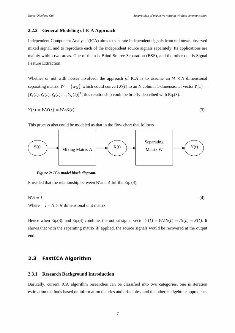
This process also could be modeled as that in the flow chart that follows

Figure 2: ICA model block diagram.

Provided that the relationship between 𝑊and 𝐴 fulfills Eq. (4).

𝑊𝐴 = 𝐼 (4)

Where 𝐼 = 𝑁 × 𝑁 dimensional unit matrix

Hence when Eq.(3). and Eq.(4) combine, the output signal vector 𝑌(𝑡) = 𝑊𝐴𝑆(𝑡) = 𝐼𝑆(𝑡) = 𝑆(𝑡). It

shows that with the separating matrix 𝑊 applied, the source signals would be recovered at the output

end.

2.3 FastICA Algorithm

2.3.1 Research Background Introduction

Basically, current ICA algorithm researches can be classified into two categories, one is iteration

estimation methods based on information theories and principles, and the other is algebraic approaches

S(t) Y(t)

Mixing Matrix A

Separating

Matrix W X(t)


8

based on statistics. Theoriatically, both methods utilize the indepedence and non-Gaussian features of

the source signal vector.

On one hand, for those based on information theories, many estimation algorithms have been brought

out from different perspectives, such as maximum entropy method, minimum mutual information

method, maximum likelihood method and negative entropy maximization method (FastICA algorithm).

On the other hand, for those estimation algorithms based on statistics, many High Order Cumulants

relate approaches have been carried out, including second-order cumulants approach, forth-order

cumulants approach, etc.

In this article, negative entropy maximization estimation method is mainly discussed.

2.3.2 Negative Entropy Maximization Estimation Method

2.3.2.1 Step.1 Data Preprocessing

Normally, signals within the observed vector 𝑋(𝑡) correlate to each other. While for independent

component analysis, correlation could be fatal and hence influence the outcome severely. Hence before

utilizing the observed signal vector 𝑋(𝑡) to recover the original source signal vector 𝑆(𝑡) , extra

processes need to take places to rule out the correlation factors.

There are many ways to rule out the correlation parts, whereas whitening processing is the most

achievable one among those.

Whitening processing could remove the correlations between signals in the observed vector, and hence

could simplify the follow up independent component extraction process. Moreover, based on large

amount of researches [2], after coming out from exactly the same algorithm processing, results coming

out from whitened signals have better convergence than those without whitening processed.

Assume that there is a random zero mean vector 𝑍 = [𝑍1, 𝑍2, 𝑍3, … , 𝑍𝑀]𝑇. If the vector Z fulfills the Eq.

(5), then it could be called as a whitened vector.

𝐸{𝑍𝑍𝑇} = 𝐼 (5)

Where 𝐼 = unit matrix

The essential functionality of the whitening process is to remove the correlation qualities from the

signals. The primary reason of doing this is basically the same as that of applying Principal Component

Analysis.


9

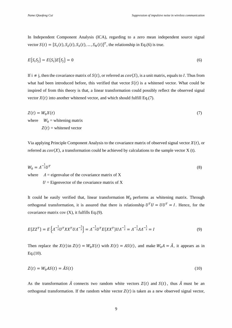
In Independent Component Analysis (ICA), regarding to a zero mean independent source signal

vector 𝑆(𝑡) = [𝑆1(𝑡), 𝑆2(𝑡), 𝑆3(𝑡), … , 𝑆𝑁(𝑡)]𝑇, the relationship in Eq.(6) is true.

𝐸{𝑆𝑖𝑆𝑗} = 𝐸{𝑆𝑖}𝐸{𝑆𝑗} = 0 (6)

If i ≠ j, then the covariance matrix of 𝑆(𝑡), or referred as 𝑐𝑜𝑣(𝑆), is a unit matrix, equals to 𝐼. Thus from

what had been introduced before, this verified that vector 𝑆(𝑡) is a whitened vector. What could be

inspired of from this theory is that, a linear transformation could possibly reflect the observed signal

vector 𝑋(𝑡) into another whitened vector, and which should fulfill Eq.(7).

𝑍(𝑡) = 𝑊0𝑋(𝑡) (7)

where 𝑊0 = whitening matrix

𝑍(𝑡) = whitened vector

Via applying Principle Component Analysis to the covariance matrix of observed signal vector 𝑋(𝑡), or

referred as 𝑐𝑜𝑣(𝑋), a transformation could be achieved by calculations to the sample vector X (t).

𝑊0 = 𝛬−1

2𝑈𝑇 (8)

where 𝛬 = eigenvalue of the covariance matrix of X

𝑈 = Eigenvector of the covariance matrix of X

It could be easily verified that, linear transformation 𝑊0 performs as whitening matrix. Through

orthogonal transformation, it is assured that there is relationship 𝑈𝑇𝑈 = 𝑈𝑈𝑇 = 𝐼 . Hence, for the

covariance matrix cov (X), it fulfills Eq.(9).

𝐸{𝑍𝑍𝑇} = 𝐸 {𝛬−1

2𝑈𝑇𝑋𝑋𝑇𝑈𝛬−1

2} = 𝛬−1

2𝑈𝑇𝐸{𝑋𝑋𝑇}𝑈𝛬−1

2 = 𝛬−1

2𝛬𝛬−1

2 = 𝐼 (9)

Then replace the 𝑋(𝑡) in 𝑍(𝑡) = 𝑊0𝑋(𝑡) with 𝑋(𝑡) = 𝐴𝑆(𝑡), and make 𝑊0𝐴 = �� , it appears as in

Eq.(10).

𝑍(𝑡) = 𝑊0𝐴𝑆(𝑡) = ��𝑆(𝑡) (10)

As the transformation �� connects two random white vectors 𝑍(𝑡) and 𝑆(𝑡) , thus �� must be an

orthogonal transformation. If the random white vector 𝑍(𝑡) is taken as a new observed signal vector,


10

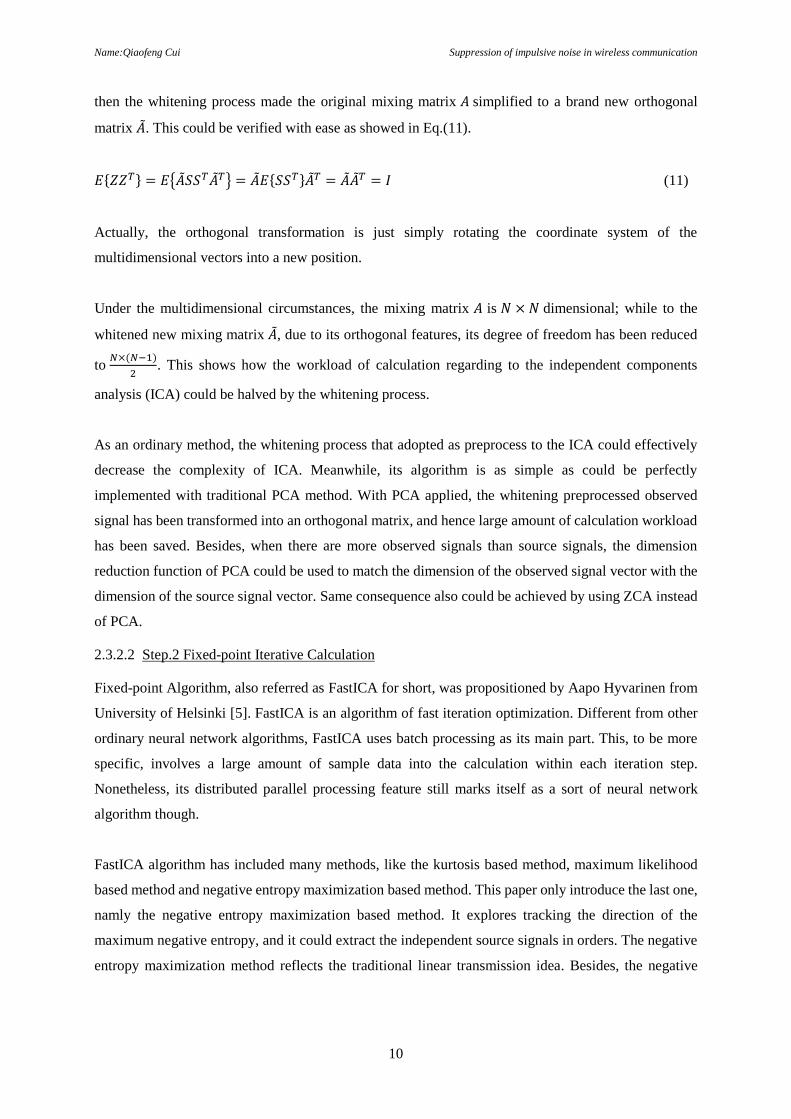
then the whitening process made the original mixing matrix 𝐴 simplified to a brand new orthogonal

matrix ��. This could be verified with ease as showed in Eq.(11).

𝐸{𝑍𝑍𝑇} = 𝐸{��𝑆𝑆𝑇��𝑇} = ��𝐸{𝑆𝑆𝑇}��𝑇 = ��𝑇 = 𝐼 (11)

Actually, the orthogonal transformation is just simply rotating the coordinate system of the

multidimensional vectors into a new position.

Under the multidimensional circumstances, the mixing matrix 𝐴 is 𝑁 × 𝑁 dimensional; while to the

whitened new mixing matrix ��, due to its orthogonal features, its degree of freedom has been reduced

to 𝑁×(𝑁−1)

2. This shows how the workload of calculation regarding to the independent components

analysis (ICA) could be halved by the whitening process.

As an ordinary method, the whitening process that adopted as preprocess to the ICA could effectively

decrease the complexity of ICA. Meanwhile, its algorithm is as simple as could be perfectly

implemented with traditional PCA method. With PCA applied, the whitening preprocessed observed

signal has been transformed into an orthogonal matrix, and hence large amount of calculation workload

has been saved. Besides, when there are more observed signals than source signals, the dimension

reduction function of PCA could be used to match the dimension of the observed signal vector with the

dimension of the source signal vector. Same consequence also could be achieved by using ZCA instead

of PCA.

2.3.2.2 Step.2 Fixed-point Iterative Calculation

Fixed-point Algorithm, also referred as FastICA for short, was propositioned by Aapo Hyvarinen from

University of Helsinki [5]. FastICA is an algorithm of fast iteration optimization. Different from other

ordinary neural network algorithms, FastICA uses batch processing as its main part. This, to be more

specific, involves a large amount of sample data into the calculation within each iteration step.

Nonetheless, its distributed parallel processing feature still marks itself as a sort of neural network

algorithm though.

FastICA algorithm has included many methods, like the kurtosis based method, maximum likelihood

based method and negative entropy maximization based method. This paper only introduce the last one,

namly the negative entropy maximization based method. It explores tracking the direction of the

maximum negative entropy, and it could extract the independent source signals in orders. The negative

entropy maximization method reflects the traditional linear transmission idea. Besides, the negative


11

entropy maximization algorithm adopted the idea of an optimal algorithm, which is Fixed-point Iteration

Algorithm. This makes the convergence process much faster and more robust.

Another thing is that fastICA also could be utilized to handle projection pursuit [5]. Projection pursuit

is about how to find out lower-dimensional projections for multielement data that with highly

nongaussian qualities..

Before discussion of how to track the negative entropy maximization, an other keyword, negentropy

criteration. From the knowledge of information theories, among all those random variables with equal

variances qualities, Gaussian variables has the maximum entropy. Thus the entropy could be utilized to

estimate the quality of non-Gaussian part. Commonly the modified form of entropy, that is negentropy,

is adopted. Based on the Central Limit Theory, if there is a random variable 𝑋, which is the sum of many

independent random variables𝑆𝑖(𝑖 = 1,2,3, … 𝑁) . Provided that 𝑆𝑖 have limit mean and variance, no

matter which distribution pattern it is, the random variable 𝑋 would be more of Gaussian distribution

than 𝑆𝑖. In other words, 𝑆𝑖 will have more non-Gaussian qualities than 𝑋.

Hence, during the separation process, the inter-independency between each separated results could be

estimated via the analysis of the non-Gaussian qualities. When the time the degree of non-Gaussian has

reached the highest peak, the separation of each independent component has been accomplished.

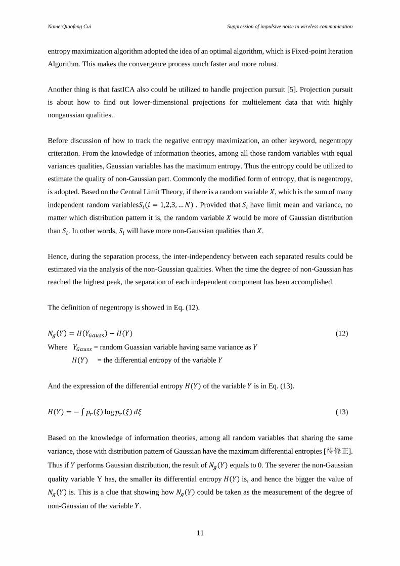
The definition of negentropy is showed in Eq. (12).

𝑁𝑔(𝑌) = 𝐻(𝑌𝐺𝑎𝑢𝑠𝑠) − 𝐻(𝑌) (12)

Where 𝑌𝐺𝑎𝑢𝑠𝑠 = random Guassian variable having same variance as 𝑌

𝐻(𝑌) = the differential entropy of the variable 𝑌

And the expression of the differential entropy 𝐻(𝑌) of the variable 𝑌 is in Eq. (13).

𝐻(𝑌) = − ∫ 𝑝𝑟(𝜉) log 𝑝𝑟(𝜉) 𝑑𝜉 (13)

Based on the knowledge of information theories, among all random variables that sharing the same

variance, those with distribution pattern of Gaussian have the maximum differential entropies [待修正].

Thus if 𝑌 performs Gaussian distribution, the result of 𝑁𝑔(𝑌) equals to 0. The severer the non-Gaussian

quality variable Y has, the smaller its differential entropy 𝐻(𝑌) is, and hence the bigger the value of

𝑁𝑔(𝑌) is. This is a clue that showing how 𝑁𝑔(𝑌) could be taken as the measurement of the degree of

non-Gaussian of the variable 𝑌.


12

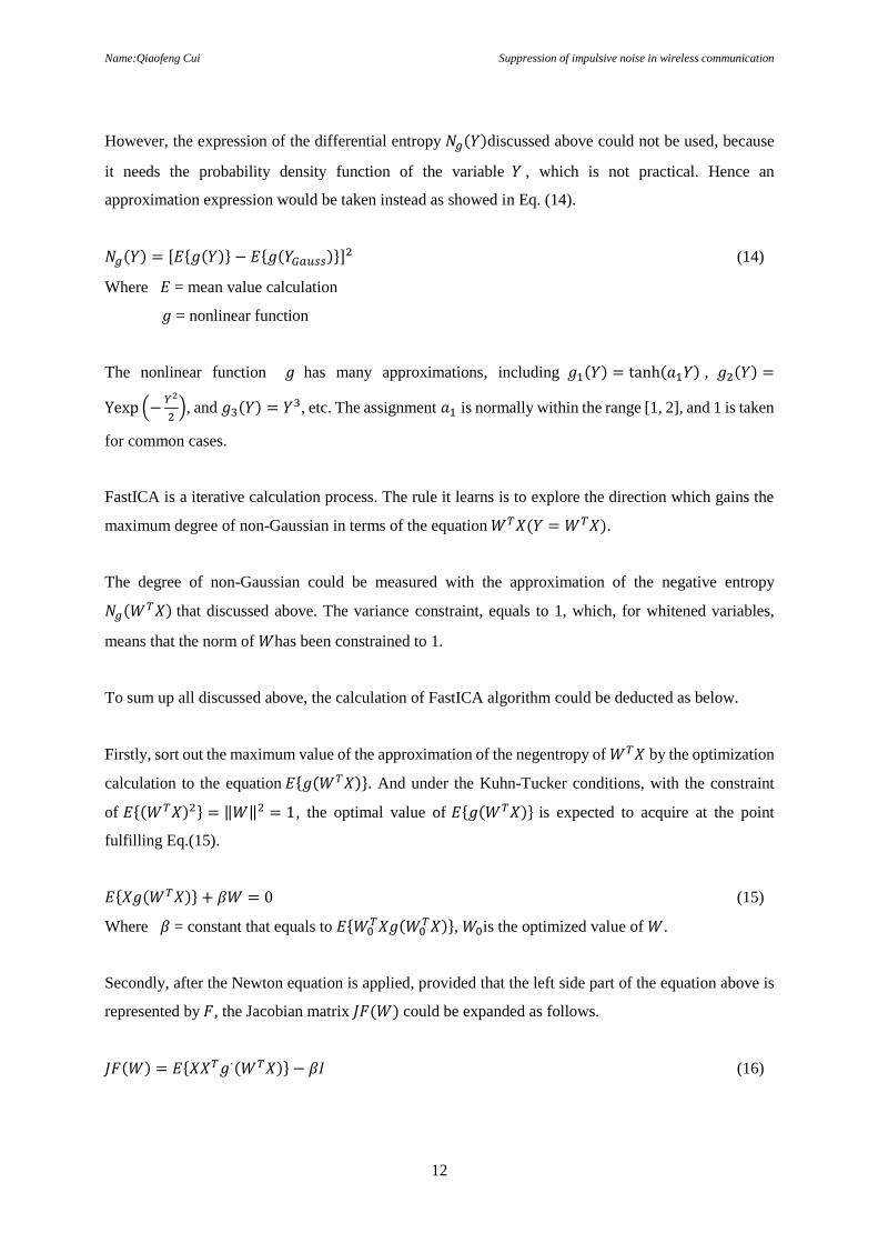
However, the expression of the differential entropy 𝑁𝑔(𝑌)discussed above could not be used, because

it needs the probability density function of the variable 𝑌 , which is not practical. Hence an

approximation expression would be taken instead as showed in Eq. (14).

𝑁𝑔(𝑌) = [𝐸{𝑔(𝑌)} − 𝐸{𝑔(𝑌𝐺𝑎𝑢𝑠𝑠)}]2 (14)

Where 𝐸 = mean value calculation

𝑔 = nonlinear function

The nonlinear function 𝑔 has many approximations, including 𝑔1(𝑌) = tanh(𝑎1𝑌) , 𝑔2(𝑌) =

Yexp (−𝑌2

2), and 𝑔3(𝑌) = 𝑌3, etc. The assignment 𝑎1 is normally within the range [1, 2], and 1 is taken

for common cases.

FastICA is a iterative calculation process. The rule it learns is to explore the direction which gains the

maximum degree of non-Gaussian in terms of the equation 𝑊𝑇𝑋(𝑌 = 𝑊𝑇𝑋).

The degree of non-Gaussian could be measured with the approximation of the negative entropy

𝑁𝑔(𝑊𝑇𝑋) that discussed above. The variance constraint, equals to 1, which, for whitened variables,

means that the norm of 𝑊has been constrained to 1.

To sum up all discussed above, the calculation of FastICA algorithm could be deducted as below.

Firstly, sort out the maximum value of the approximation of the negentropy of 𝑊𝑇𝑋 by the optimization

calculation to the equation 𝐸{𝑔(𝑊𝑇𝑋)}. And under the Kuhn-Tucker conditions, with the constraint

of 𝐸{(𝑊𝑇𝑋)2} = ‖𝑊‖2 = 1, the optimal value of 𝐸{𝑔(𝑊𝑇𝑋)} is expected to acquire at the point

fulfilling Eq.(15).

𝐸{𝑋𝑔(𝑊𝑇𝑋)} + 𝛽𝑊 = 0 (15)

Where 𝛽 = constant that equals to 𝐸{𝑊0𝑇𝑋𝑔(𝑊0

𝑇𝑋)}, 𝑊0is the optimized value of 𝑊.

Secondly, after the Newton equation is applied, provided that the left side part of the equation above is

represented by 𝐹, the Jacobian matrix 𝐽𝐹(𝑊) could be expanded as follows.

𝐽𝐹(𝑊) = 𝐸{𝑋𝑋𝑇𝑔·(𝑊𝑇𝑋)} − 𝛽𝐼 (16)


13

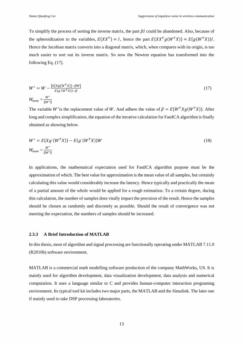
To simplify the process of sorting the inverse matrix, the part 𝛽𝐼 could be abandoned. Also, because of

the spheroidization to the variables, 𝐸{𝑋𝑋𝑇} = 𝐼 , hence the part 𝐸{𝑋𝑋𝑇𝑔(𝑊𝑇𝑋)} ≈ 𝐸{𝑔(𝑊𝑇𝑋)}𝐼 .

Hence the Jacobian matrix converts into a diagonal matrix, which, when compares with its origin, is too

much easier to sort out its inverse matrix. So now the Newton equation has transformed into the

following Eq. (17).

𝑊∗ = 𝑊 −[𝐸{𝑋𝑔(𝑊𝑇𝑋)}−𝛽𝑊]

𝐸{𝑔·(𝑊𝑇𝑋)}−𝛽 (17)

𝑊𝑛𝑒𝑤 = 𝑊∗

‖𝑊∗‖

The variable 𝑊∗is the replacement value of 𝑊. And adhere the value of 𝛽 = 𝐸{𝑊𝑇𝑋𝑔(𝑊𝑇𝑋)}. After

long and complex simplification, the equation of the iterative calculation for FastICA algorithm is finally

obtained as showing below.

𝑊∗ = 𝐸{𝑋𝑔·(𝑊𝑇𝑋)} − 𝐸{𝑔·(𝑊𝑇𝑋)}𝑊 (18)

𝑊𝑛𝑒𝑤 = 𝑊∗

‖𝑊∗‖

In applications, the mathematical expectation used for FastICA algorithm purpose must be the

approximation of which. The best value for approximation is the mean value of all samples, but certainly

calculating this value would considerably increase the latency. Hence typically and practically the mean

of a partial amount of the whole would be applied for a rough estimation. To a certain degree, during

this calculation, the number of samples does vitally impact the precision of the result. Hence the samples

should be chosen as randomly and discretely as possible. Should the result of convergence was not

meeting the expectation, the numbers of samples should be increased.

2.3.3 A Brief Introduction of MATLAB

In this thesis, most of algorithm and signal processing are functionally operating under MATLAB 7.11.0

(R2010b) software environment.

MATLAB is a commercial math modelling software production of the company MathWorks, US. It is

mainly used for algorithm development, data visualization development, data analysis and numerical

computation. It uses a language similar to C and provides human-computer interaction programing

environment. Its typical tool kit includes two major parts, the MATLAB and the Simulink. The later one

if mainly used to take DSP processing laboratories.


14

MATLAB is the combination of two words: matrix and laboratory. It is particularly skillful in matrix

computations, data plotting and digital signal processing.

In this thesis, most of results and calculation processes are illustrated either in pictures plotted by

MATLAB or the source code written in .m files.

Nowadays, the needs of the Global Positioning System, or GPS receivers, have been surging within the

urban and rural areas. Many communication applications, including both indoor and outdoor services,

have been invented. Also, as many efforts as possible have been taken by people to improve the accuracy

of our positioning systems. Among those obstacles remaining unsolved, noises have always been a great

concern. Generally, noise or interference sources received by GPS receivers are assumed to have

Gaussian or non-Gaussian distributions. These sources, including impulsive noise, ultra-wideband

(UWB) signals, and impulse and noise radar signals for target tracking and indoor imaging applications,

would interfere the GPS signals and introduce troubles to the receiver delay lock loops (DLL), giving

fatal errors in the satellite tracking phase.

Thus, of great importance, the elimination of impulsive noise in GPS has become a very vital technology

to evaluate the quality and performance of the GPS receiver device.

2.4 BPSK Modulation in GPS

At the GPS transmitter end, the data to be sent is modulated by BPSK method before the broadcasting

worldwide.

The GPS signal includes two signals that could be differentiated by its carrier frequencies. Signal L1

and L2 are at frequencies of 1575.42MHz and 1227.60MHz, respectively. The basic navigation data,

including the sending time and the constellation information of the satellite, is carried by the both signals.

Two spreading sequences, C/A code and P code, are applied to the BPSK modulations. But for the

alleged Standard Positioning Service (SPS) that provided through the L1 signal, only the C/A code is

applied. Thus, as the interfere of the impulsive noises applied to either L1 signal or L2 signal are the

same, to make simplicity in this research, only the Standard Positioning Service (SPS), which is

modulated by BPSK method with the C/A code and carried by the L1 signal of 1575.42MHz, is

considered.


15

The complete GPS transmitter system is showed in the following figure. This figure is acquired from

the ‘SoftGNSS’ Project and recorded into the book ‘A Software-defined GPS & Galileo Receiver’, by

Kai Borre & Dennis M .Akos, 2007.

Figure 3: The Generation of GPS Signals At The Satellites. (From SoftGNSS Project)

Figure 4: The Waveform of L1 GPS Signals and Its Components. (From SoftGNSS Project)

In this figure, the wave C indicates the C/A code, whereas the wave D indicates the data sequence to be

sent. After when the C/A code and the data are combined together by a simple exclusive OR operation,

the combined signal is modulated with the 1575.2 MHz carrier signal by the BPSK modulator.


16

3 Simulation and Results

In this chapter, the full processing procedures are discussed. During the discussion, according codes in

MATLAB are attached with printed results. The full source coding is also attached in the appendix parts

at the last pages of the thesis.

The results are showed in pictures plotted by MATLAB to illustrate the effect that the fastICA imposed

on the observation signal vector. All the waveforms, including the original source information source

signal, the sampled discrete digitalized signal vector, the impulsive noise image, the mixed observation

signal vector, the centralized signal, the whitened signal, the separating matrix and the separated final

output, are exhibited and compared in details.

Further problems and analysis to the results are involved in the next chapter.

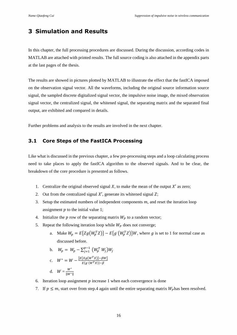
3.1 Core Steps of the FastICA Processing

Like what is discussed in the previous chapter, a few pre-processing steps and a loop calculating process

need to take places to apply the fastICA algorithm to the observed signals. And to be clear, the

breakdown of the core procedure is presented as follows.

1. Centralize the original observed signal 𝑋, to make the mean of the output 𝑋′ as zero;

2. Out from the centralized signal 𝑋′, generate its whitened signal 𝑍;

3. Setup the estimated numbers of independent components 𝑚, and reset the iteration loop

assignment 𝑝 to the initial value 1;

4. Initialize the 𝑝 row of the separating matrix 𝑊𝑃 to a random vector;

5. Repeat the following iteration loop while 𝑊𝑃 does not converge;

a. Make 𝑊𝑝 = 𝐸{𝑍𝑔(𝑊𝑝𝑇𝑍)} − 𝐸{𝑔·(𝑊𝑝

𝑇𝑍)}𝑊, where 𝑔 is set to 1 for normal case as

discussed before.

b. 𝑊𝑝 = 𝑊𝑝 − ∑ (𝑊𝑝𝑇 𝑊𝑗)𝑊𝑗

𝑝−1𝑗=1

c. 𝑊∗ = 𝑊 −[𝐸{𝑋𝑔(𝑊𝑇𝑋)}−𝛽𝑊]

𝐸{𝑔·(𝑊𝑇𝑋)}−𝛽

d. 𝑊 = 𝑊∗

‖𝑊∗‖

6. Iteration loop assignment 𝑝 increase 1 when each convergence is done

7. If 𝑝 ≤ 𝑚, start over from step.4 again until the entire separating matrix 𝑊𝑃has been resolved.


17

To be clear, the procedure from step 1 to step 2 is named as Preprocessing; steps 3 is called as

Initialization; the core part from step 4 to 7 is referred as the Iteration Loop in the following paragraphs.

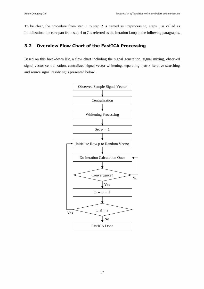
3.2 Overview Flow Chart of the FastICA Processing

Based on this breakdown list, a flow chart including the signal generation, signal mixing, observed

signal vector centralization, centralized signal vector whitening, separating matrix iterative searching

and source signal resolving is presented below.

Observed Sample Signal Vector

Centralization

Whitening Processing

Convergence?

Set 𝑝 = 1

Initialize Row 𝑝 to Random Vector

Do Iteration Calculation Once

𝑝 = 𝑝 + 1

𝑝 ≤ 𝑚?

FastICA Done

Yes

Yes

No

No


18

Figure 5: The Overview Flow Chart of The FastICA Application

3.3 Generation of Signals

Before forwarding into the more detailed steps of the fastICA processing, the features of the source

signals that has been used are introduced. To get up closer to the background of industrial applications,

BPSK modulated signals and impulsive noise signals are selected. Impulsive noise is very normal to see

in industrial environment. They could be generated by motors, vehicles and other repeating operational

machinaries. And while it comes to wireless communication, this kind of noise also could be added to

the main source signals through its electromagnetic energy, and thus it interferred the receiver from the

extraction of primary information.

To research the effects that the fastICA algorithm applys to the modern digital modulated signals that

mixed with impulsive noises, these two signals are generated in mathmatic modelings introduced in the

following segments.

3.3.1 Generation of BPSK Modulated Signals

Of the three different ways that commonly used within the digital modulation field, namly ASK, FSK,

PSK, PSK is the one using variations in the phase of the carrier to deliver the information. Comparing

with ASK and FSK, the PSK has the best performance in noise proof ability and signal spectrum

utilization and is extensively used in high speed transmission systems. And among all mature PSK

featured technologies, including BPSK, QPSK, 8PSK and so forth, BPSK has been the most basic and

simpliest one. It has the best noise proof characteristics but also the lowest transmission efficiency.

3.3.1.1 Binary Phase Shift Keying (BPSK)

In BPSK modulation, the local carrier is used in two phases to indicate the data change in binary

mechanism. Normally a keying switch between carriers with inverted phases ’θ = 0’ and ’θ = π’ is

adopted to convert the ’zeros’ and ’ones’ in digital data streams into radiative frequencies.

The expression of BPSK modulated signals in time domain is as follows.

𝑢𝑚(𝑡) = 𝐴𝑔𝑇(𝑡) cos(2𝜋𝑓𝑐𝑡 + 𝜃) (19)

Where 𝑓𝑐 = the frequency of the carrier signal

𝜃 = 0 while sending ‘zero’; 1 while sending ‘one’

𝑔𝑇(𝑡) =√2𝜀𝑚

𝑇 , a gate signal (or a pulse) with total energy of 𝜀𝑚


19

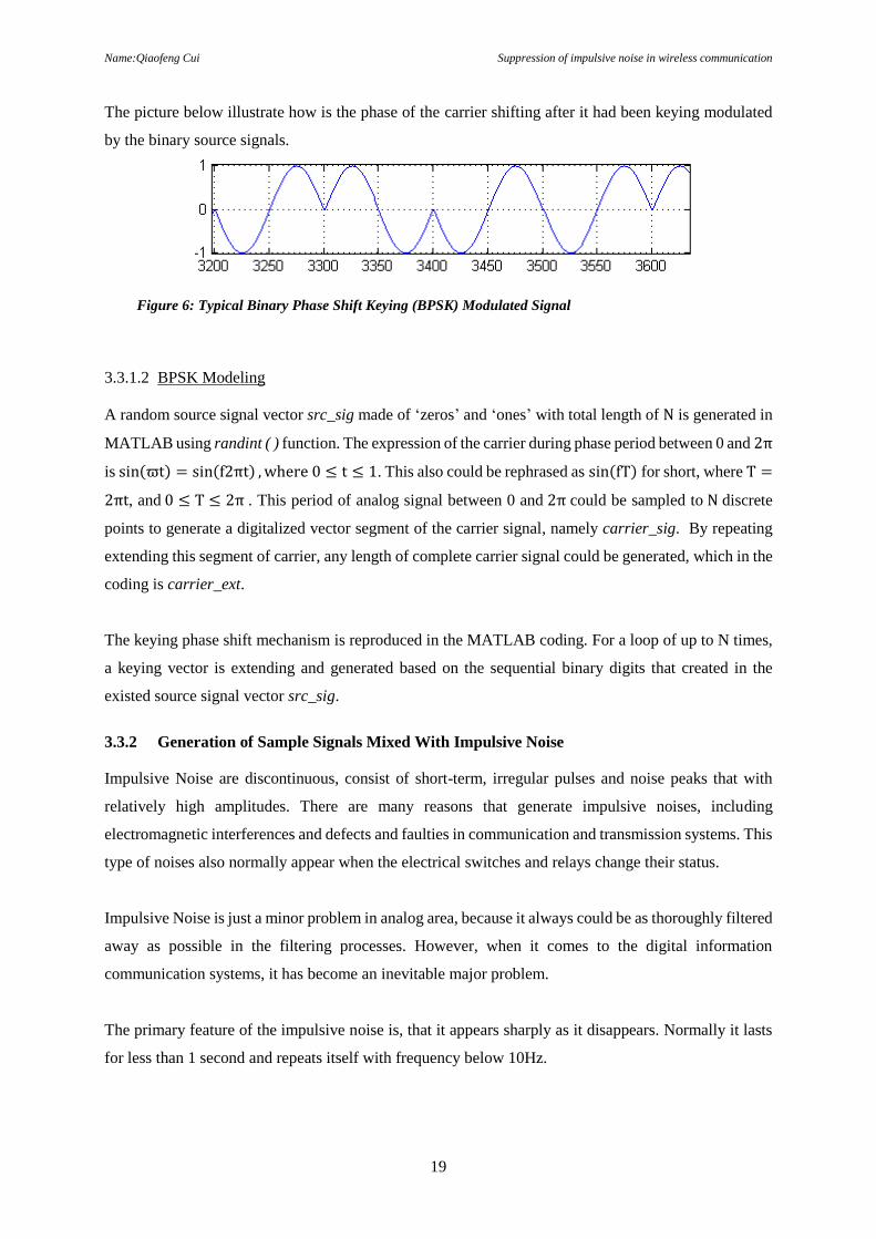
The picture below illustrate how is the phase of the carrier shifting after it had been keying modulated

by the binary source signals.

Figure 6: Typical Binary Phase Shift Keying (BPSK) Modulated Signal

3.3.1.2 BPSK Modeling

A random source signal vector src_sig made of ‘zeros’ and ‘ones’ with total length of N is generated in

MATLAB using randint ( ) function. The expression of the carrier during phase period between 0 and 2π

is sin(ϖt) = sin(f2πt) , where 0 ≤ t ≤ 1. This also could be rephrased as sin(fT) for short, where T =

2πt, and 0 ≤ T ≤ 2π . This period of analog signal between 0 and 2π could be sampled to N discrete

points to generate a digitalized vector segment of the carrier signal, namely carrier_sig. By repeating

extending this segment of carrier, any length of complete carrier signal could be generated, which in the

coding is carrier_ext.

The keying phase shift mechanism is reproduced in the MATLAB coding. For a loop of up to N times,

a keying vector is extending and generated based on the sequential binary digits that created in the

existed source signal vector src_sig.

3.3.2 Generation of Sample Signals Mixed With Impulsive Noise

Impulsive Noise are discontinuous, consist of short-term, irregular pulses and noise peaks that with

relatively high amplitudes. There are many reasons that generate impulsive noises, including

electromagnetic interferences and defects and faulties in communication and transmission systems. This

type of noises also normally appear when the electrical switches and relays change their status.

Impulsive Noise is just a minor problem in analog area, because it always could be as thoroughly filtered

away as possible in the filtering processes. However, when it comes to the digital information

communication systems, it has become an inevitable major problem.

The primary feature of the impulsive noise is, that it appears sharply as it disappears. Normally it lasts

for less than 1 second and repeats itself with frequency below 10Hz.


20

To generate a simplest impulsive noise with same length as that of the BPSK modulated signal vector

bpsk_sig, just use one line of coding in MATLAB.

This impulsive noise signal is not very close to natural noises in shape. Actually a noise signal mixed

up with two or more impulsive noise signals of variant amplitude would be more of reality and value to

research. To achieve this, a more complex noise signal made up from two intermodulated different

impulsive noise signals is coded.

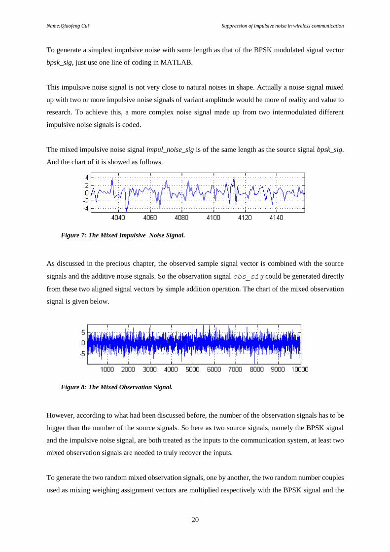
The mixed impulsive noise signal impul_noise_sig is of the same length as the source signal bpsk_sig.

And the chart of it is showed as follows.

Figure 7: The Mixed Impulsive Noise Signal.

As discussed in the precious chapter, the observed sample signal vector is combined with the source

signals and the additive noise signals. So the observation signal obs_sig could be generated directly

from these two aligned signal vectors by simple addition operation. The chart of the mixed observation

signal is given below.

Figure 8: The Mixed Observation Signal.

However, according to what had been discussed before, the number of the observation signals has to be

bigger than the number of the source signals. So here as two source signals, namely the BPSK signal

and the impulsive noise signal, are both treated as the inputs to the communication system, at least two

mixed observation signals are needed to truly recover the inputs.

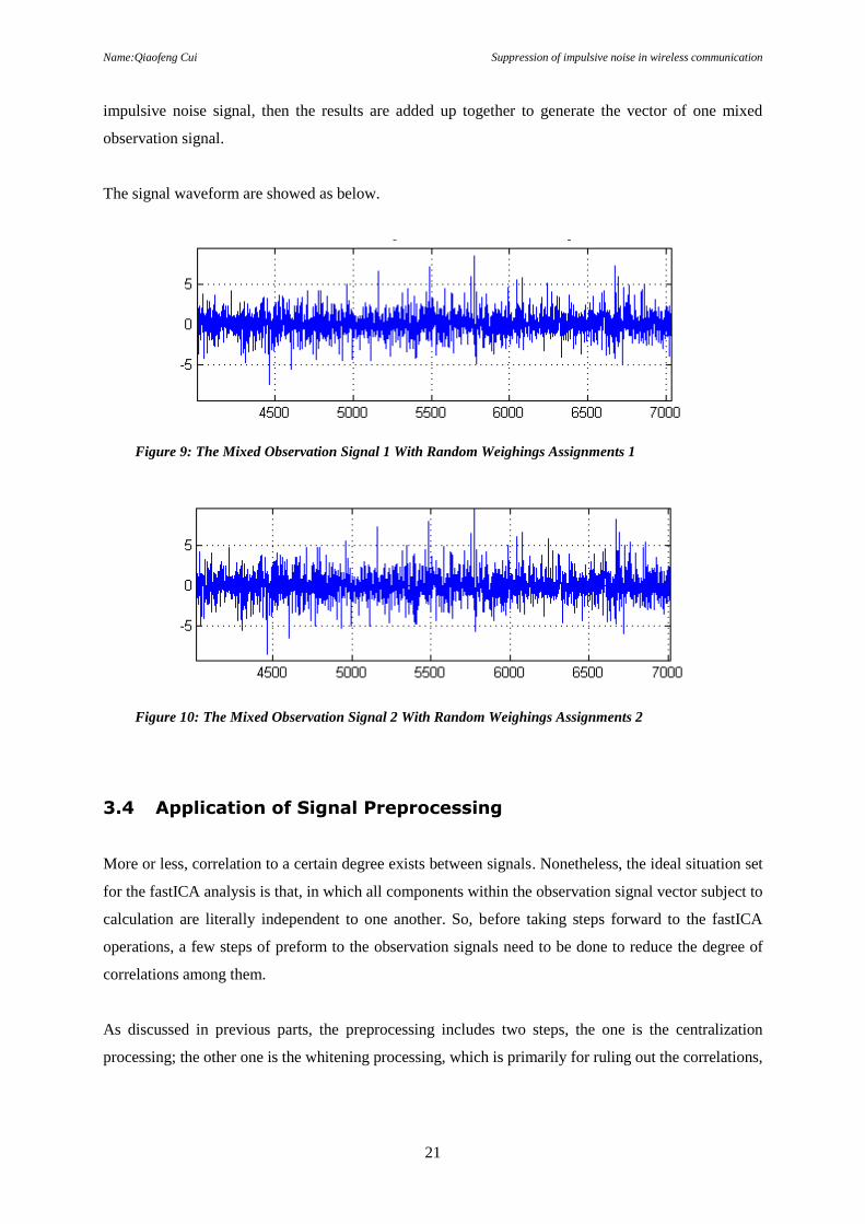
To generate the two random mixed observation signals, one by another, the two random number couples

used as mixing weighing assignment vectors are multiplied respectively with the BPSK signal and the


21

impulsive noise signal, then the results are added up together to generate the vector of one mixed

observation signal.

The signal waveform are showed as below.

Figure 9: The Mixed Observation Signal 1 With Random Weighings Assignments 1

Figure 10: The Mixed Observation Signal 2 With Random Weighings Assignments 2

3.4 Application of Signal Preprocessing

More or less, correlation to a certain degree exists between signals. Nonetheless, the ideal situation set

for the fastICA analysis is that, in which all components within the observation signal vector subject to

calculation are literally independent to one another. So, before taking steps forward to the fastICA

operations, a few steps of preform to the observation signals need to be done to reduce the degree of

correlations among them.

As discussed in previous parts, the preprocessing includes two steps, the one is the centralization

processing; the other one is the whitening processing, which is primarily for ruling out the correlations,


22

and hence would simplify the following fastICA processing by providing better convergence speed and

result.

3.4.1 Centralization Processing

Before move on to the whitening processing step, the observation signal vector need to be centralized,

which, in other words, is to make the mean of the observation signal vector align to zero.

To achieve this, the mean of all discrete numbers within the vecotr need to be calculated, and then each

of them need to minus themselves with it. This kind of calculation could be a extramely boring treadmill,

but fortunately it would be done by the in-built function embedded in MATLAB.

Hence after this, the distribution of data within the centralized signal would be rearranged evenly

arround the both sides of the axis.

Provided that this step is skipped in the operation, the result is still obtainable, but just more calculation

and time are need to figure out. So, this step is taken only for the purpose of simplifying the calculation

operations. Actually, the mean value also could be extimated by the algorithm.

3.4.2 Whitening Processing

The whitening processing is acomplished in traditional PCA method. As the most popular method, on

one hand, the PCA calculation to the vector would move out the correlation factors of the centralized

observation signal vector and hence improve the convergence speed and result as consequence; On the

other hand, since the PCA method is a very good way to reduce the noise and dimensionality of the

vector, the data after compression would have the minimum mean square deviation, which equals to the

sum of all cut-off eigenvalues. On the other side, though some of the information might get lost in the

whitening processing, the majority still remains. This is because that, if all eigenvalues are sorted in

ascending order, reservation of initial multiple figures could still keep the most part of the energies of

the original observation signals.

There are two very important conditions that must be met before going further to the whitening

processing. One is that the correlation between different eigenvalues is minimum, close to 0, the other

is that the variances across all eigenvalues must be equal to each other.

After the PCA processed signal applied to the whitening processing, the whitened observation signal

would be converted to an orthogonal form. This form of matrix could reduce the iteration times during

the calculation loop. Also, by applying the whitening processing, the variances of all whitened

components would be changed to one, and this makes them to have equal variances.


23

Also, if the number of observation signals is bigger than that of the source signals that are over to be

resolved, the PCA processing could downsize the observation signal to match its dimensions to the

source signal vectors.

To calculate the PCA matrix for the centralized observation signal vector, the covariance of the

observation signal need to be calculated at first. Then the eigenvalues D and eigenvectors E of the

covariance matrix could be resolved with the inbuilt cov( ) function. The whitening matrix is built based

on the eigenvalues and the eigenvectors of the covariance matrix. Using the equation that had been

discussed before, 𝑊0 = 𝛬−1

2𝑈𝑇, where 𝛬 is the eigenvalue of the covariance matrix covarianceMatrix

and the 𝑈 is the eigenvector of the covariance matrix covarianceMatrix. Finally the centralized signal

that obtained from the previous process would be applied to the whitening matrix and get whitened. The

result of whitening processing is named as white_sig in the coding.

There it also could have another side-effect generated in this step. During the use of PCA in this

processing, if the eigenvalue of the covarianceMatrix, or D as showing in the coding, is sorted in

descending order, a cut-off line that representing the proportion between other eigenvalues to the largest

eigenvalues could be easily sorted out. With this cut-off line, a new eigenvalue vector including only

values over this line could be reformed and utilized instead. This new eigenvalue vector would have a

narrowed dimensionality, and so the dimensionality of the whitened signal has also be reduced after the

whitening processing has been applied. Actually, when the number of observation signals is larger than

the number of source signals, with the whitening processing, the dimensionality of the whitened signal

will decrease from the number of observation vectors to the number of source vectors. Hence many

more rounds of iteration calculation loops in the following steps could be saved, especially when there

are many more groups of observation data than groups of source data.

After the whitening processing, the correlation across observation signal vectors has been removed. The

basic requirement of independent component analysis has been prepared.

Notice that the rank of the final separated signal vectors would be influenced by the form of eigenvalues

and eigenvectors. If sorting work is not taken in this procedure, the outcome of the fastICA processed

signals could be in any random order. Also sometimes it will lead to separated signals that inverted to

the source signal. Normally in real applications, this would not interfere the analysis to the original

source signals.

If the whitening is successful, there is a way to verify the result. Since the whitening processing is used

to rule out the correlation factors between the observation signals, if it is successful, the result out


24

coming from it should be not correlated to each other. That is to say, as that had been discussed in

previous chapter, the covariance of the matrix constitute of all whitened signals should be a unit matrix.

3.5 Application of Fixed-point Iterative Calculation

3.5.1 FastICA Iteration Loop

Before it dives into the iteration loop, some initialization work should be done. For example, the

maximum iteration times should be set to abort the loop when it comes to abnormal conditions.

The value of the max_interation is the maximum iteration times set for breaking am undergoing loop.

In the ideal case, this value should be set to infinite. But as the computing ability of the computers is

limited, a finite value should be given to avoid the program get stuck in the iteration loop.

Normally, for ‘fast’ ICA, the iteration times would be expected to be in a range that less than 10.

Nonetheless, this does not guarantee that no iteration loop numbers would exceed this number. So, in

this application, the max_interation is set to 100, which is much greater than the need for common

iteration loops, but also could assure the calculation would not hang on in the loops.

In the iteration loop, for calculation of each single row of separating matrix B, firstly a vector of random

values are set to the p row of separating matrix B for initialization, and then a normalization is applied

to set all numbers in the p row ( marked as separating vector b) to a range from 0 to 1.

The normalization processing would make the separated vector to have unit energy.

To make all numbers in the row of separating vector b fall into the range within 0 to 1, the 2-norm value

of all numbers in the separating vector b is initially calculated. The mathematic representation of the 2-

norm function is showed below.

2𝑛𝑜𝑟𝑚(𝑏) = √𝑛12 + 𝑛2

2 + ⋯ + 𝑛𝑛2 (20)

where b = (𝑛1,, 𝑛2, … , 𝑛𝑛)

After this, as the 2-norm value of all umbers within the vector must be positive and not less than each

of the numbers within the vector, if each number within the vector is divided by thier 2-norm value, the

results must be proper fractions. In other words, by applying numbers over 2-norm operations, the

numbers could be replaced by a new number within range between 0 and 1. The mathematic

representation of this is present as follows.


25

𝑏′ =𝑛1,

2𝑛𝑜𝑟𝑚(𝑏),

𝑛2,

2𝑛𝑜𝑟𝑚(𝑏), … ,

𝑛𝑛,

2𝑛𝑜𝑟𝑚(𝑏)

=𝑛1,

√𝑛12+𝑛2

2+⋯+𝑛𝑛2

,𝑛2,

√𝑛12+𝑛2

2+⋯+𝑛𝑛2

, … ,𝑛𝑛,

√𝑛12+𝑛2

2+⋯+𝑛𝑛2 (21)

where b = (𝑛1,, 𝑛2, … , 𝑛𝑛)

This processing could be very vital and of great convinience for the later on processings. This is because

only when ‖𝑏‖2 = 𝑏12 + 𝑏2

2 + ⋯ + 𝑏𝑛2 = 1, the variance equals to 1 as well, which is the same as the

setting to the signal that is going to be processed; hence the approximation of the maximum negentropy

could be used instead based on Kuhn-Tucker conditions, which makes it possible to solve the maximum

value of the negentropy.

After the normalization processing, for b, there is relationship

‖𝑏‖2 = 𝑏12 + 𝑏2

2 + ⋯ + 𝑏𝑛2

=𝑛1

2

(√𝑛12 + 𝑛2

2 + ⋯ + 𝑛𝑛2)

2 +𝑛2

2

(√𝑛12 + 𝑛2

2 + ⋯ + 𝑛𝑛2)

2 + ⋯ +𝑛𝑛

2

(√𝑛12 + 𝑛2

2 + ⋯ + 𝑛𝑛2)

2

=𝑛1

2+𝑛22+⋯+𝑛𝑛

2

𝑛12+𝑛2

2+⋯+𝑛𝑛2 = 1.

Then the core equation applies to the vectors, once each time. Then after the operation of the core

equation, another round of orthogonalization and normalization is necessary to take place.

Principally, by looping the operation discussed above again and again, using different random initial

separating vector at the beginning for each time, it is enough already to extract each independent source

vector out from the observation signal. However, as many approximations have been used in our

operation to simplify the algorithm and save operation durations, including the adoption instead of

expectation and so forth, the error gap will roll itself up and get bigger and bigger as snowballs starting

from the approximation of the first source vector. This effect would considerably influence the

separation process and the final results.

To make up this default, normally an orthogonalization processing would be added on to the next stage

of the whole iteration loop. With such method, the approximations of the separating vectors do not get

extracted in a row but in parallel. To be more specific, firstly the similar iteration calculation loop steps

will take place to each vector in parallel, and then they get orthogonalization processing in some special

symmetry order.


26

The loop ends with the comparison of the achieved vector to its number at the last time in the iterative

loop to decide if it is converge. If the vector has converged, break the loop and store the vector; If the

vector has yet converged, before the loop times reach the maxmum iteration times parameter, the loop

continues.

After the separation matrix has been resolved. The separated signals could be recovered with just one

line of coding as showing below.

Ica = B * whitening_matrix * obs_sigs ;

The signal scopes and result analysis are discussed in the following chapters.

3.6 Visual Plotting and Results

MATLAB has provided very functional built-in data visualization simulation scopes to use. Signals,

data and other information could be illustrated and analyzed in any aspects.

In this thesis, the distinguishing of signal vectors is the most concern.

There are two different signal vectors that generated at the starting point of this thesis. To be compared

at the end with the recovered signals, these original data are stored and firstly illustrated with the

commands.

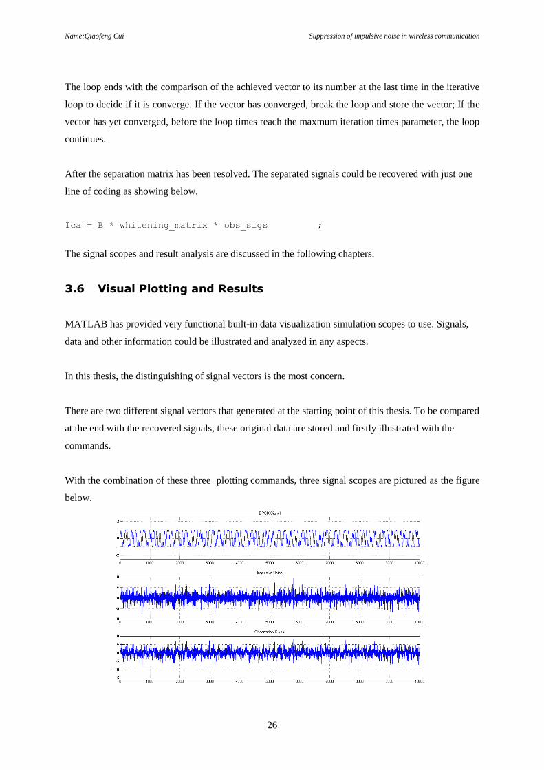
With the combination of these three plotting commands, three signal scopes are pictured as the figure

below.


27

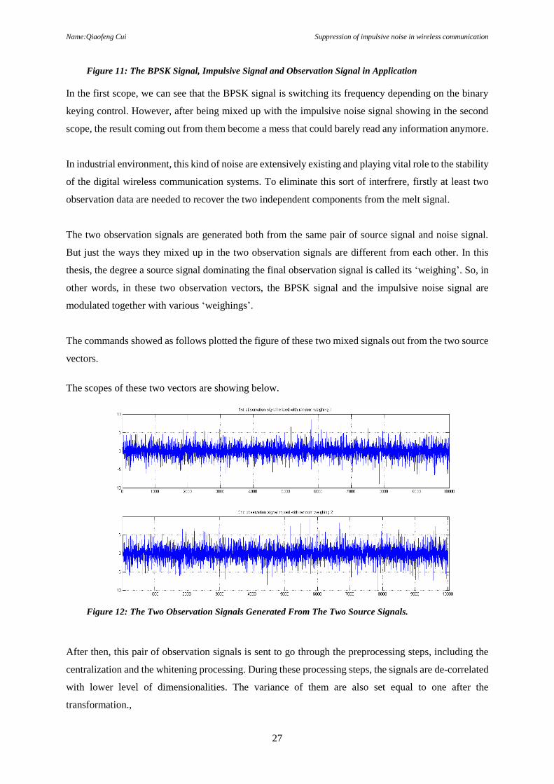
Figure 11: The BPSK Signal, Impulsive Signal and Observation Signal in Application

In the first scope, we can see that the BPSK signal is switching its frequency depending on the binary

keying control. However, after being mixed up with the impulsive noise signal showing in the second

scope, the result coming out from them become a mess that could barely read any information anymore.

In industrial environment, this kind of noise are extensively existing and playing vital role to the stability

of the digital wireless communication systems. To eliminate this sort of interfrere, firstly at least two

observation data are needed to recover the two independent components from the melt signal.

The two observation signals are generated both from the same pair of source signal and noise signal.

But just the ways they mixed up in the two observation signals are different from each other. In this

thesis, the degree a source signal dominating the final observation signal is called its ‘weighing’. So, in

other words, in these two observation vectors, the BPSK signal and the impulsive noise signal are

modulated together with various ‘weighings’.

The commands showed as follows plotted the figure of these two mixed signals out from the two source

vectors.

The scopes of these two vectors are showing below.

Figure 12: The Two Observation Signals Generated From The Two Source Signals.

After then, this pair of observation signals is sent to go through the preprocessing steps, including the

centralization and the whitening processing. During these processing steps, the signals are de-correlated

with lower level of dimensionalities. The variance of them are also set equal to one after the

transformation.,


28

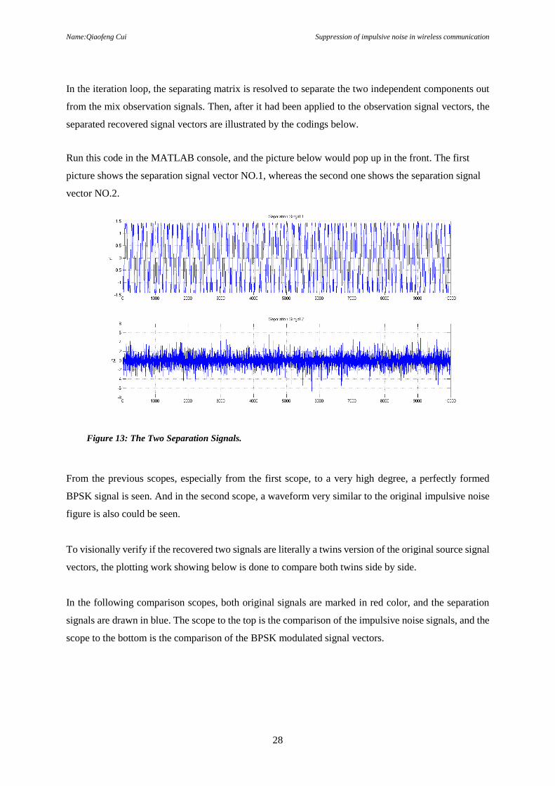
In the iteration loop, the separating matrix is resolved to separate the two independent components out

from the mix observation signals. Then, after it had been applied to the observation signal vectors, the

separated recovered signal vectors are illustrated by the codings below.

Run this code in the MATLAB console, and the picture below would pop up in the front. The first

picture shows the separation signal vector NO.1, whereas the second one shows the separation signal

vector NO.2.

Figure 13: The Two Separation Signals.

From the previous scopes, especially from the first scope, to a very high degree, a perfectly formed

BPSK signal is seen. And in the second scope, a waveform very similar to the original impulsive noise

figure is also could be seen.

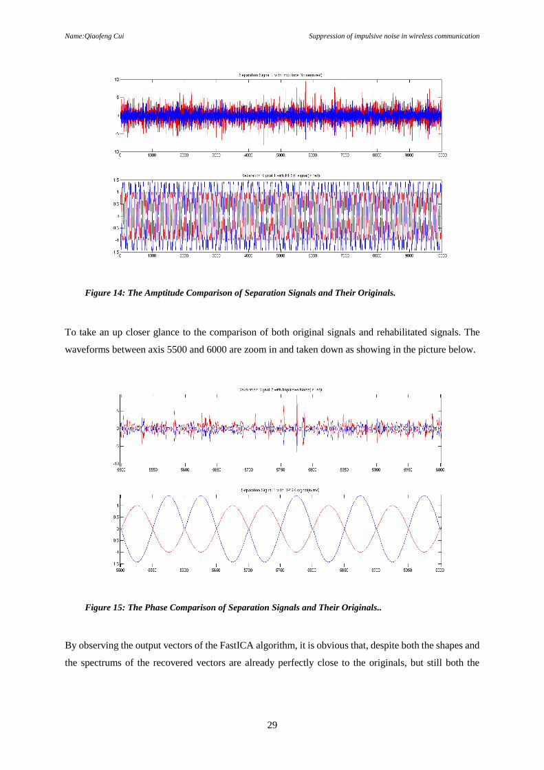
To visionally verify if the recovered two signals are literally a twins version of the original source signal

vectors, the plotting work showing below is done to compare both twins side by side.

In the following comparison scopes, both original signals are marked in red color, and the separation

signals are drawn in blue. The scope to the top is the comparison of the impulsive noise signals, and the

scope to the bottom is the comparison of the BPSK modulated signal vectors.


29

Figure 14: The Amptitude Comparison of Separation Signals and Their Originals.

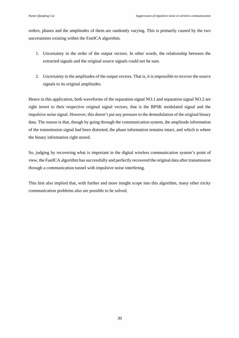
To take an up closer glance to the comparison of both original signals and rehabilitated signals. The

waveforms between axis 5500 and 6000 are zoom in and taken down as showing in the picture below.

Figure 15: The Phase Comparison of Separation Signals and Their Originals..

By observing the output vectors of the FastICA algorithm, it is obvious that, despite both the shapes and

the spectrums of the recovered vectors are already perfectly close to the originals, but still both the


30

orders, phases and the amplitudes of them are randomly varying. This is primarily caused by the two

uncertainties existing within the FastICA algorithm.

1. Uncertainty in the order of the output vectors. In other words, the relationship between the

extracted signals and the original source signals could not be sure.

2. Uncertainty in the amplitudes of the output vectors. That is, it is impossible to recover the source

signals to its original amplitudes.

Hence in this application, both waveforms of the separation signal NO.1 and separation signal NO.2 are

right invert to their respective original signal vectors, that is the BPSK modulated signal and the

impulsive noise signal. However, this doesn’t put any pressure to the demodulation of the original binary

data. The reason is that, though by going through the communication system, the amplitude information

of the transmission signal had been distorted, the phase information remains intact, and which is where

the binary information right stored.

So, judging by recovering what is important in the digital wireless communication system’s point of

view, the FastICA algorithm has successfully and perfectly recovered the original data after transmission

through a communication tunnel with impulsive noise interfering.

This hint also implied that, with further and more insight scope into this algorithm, many other tricky

communication problems also are possible to be solved.


31

4 FastICA Application to GPS

4.1 The Impact of Impulsive Noise to GPS

As the GPS signals has to travel a very long journey from the satellite to the earth before its arrival at

the receiver ends, normally the power of it has attenuated considerably and any obstacles or noises could

make very much great interferences to the GPS signal demodulation process. This is why that the

antenna part of the receiver is always suggested to be put outdoor.

To simulate the impact of the impulsive noise to the GPS receiver, the Matlab model created by the

‘SoftGNSS’ Project is used in this thesis. The SoftGNSS Project is a research project conducted by Kai

Borre from Aalborg University and Dennis M .Akos from University of Colorado, the introduction of

this model is available on http://gps.aau.dk/softgps.

The GPS signal data used in this project is collected from real resources.

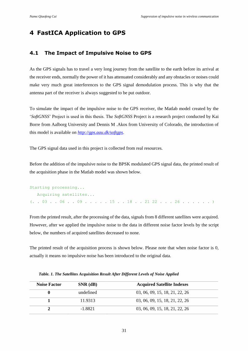
Before the addition of the impulsive noise to the BPSK modulated GPS signal data, the printed result of

the acquisition phase in the Matlab model was shown below.

Starting processing...

Acquiring satellites...

(. . 03 . . 06 . . 09 . . . . . 15 . . 18 . . 21 22 . . . 26 . . . . . . )

From the printed result, after the processing of the data, signals from 8 different satellites were acquired.

However, after we applied the impulsive noise to the data in different noise factor levels by the script

below, the numbers of acquired satellites decreased to none.

The printed result of the acquisition process is shown below. Please note that when noise factor is 0,

actually it means no impulsive noise has been introduced to the original data.

Table. 1. The Satellites Acquisition Result After Different Levels of Noise Applied

Noise Factor SNR (dB) Acquired Satellite Indexes

0 undefined 03, 06, 09, 15, 18, 21, 22, 26

1 11.9313 03, 06, 09, 15, 18, 21, 22, 26

2 -1.8821 03, 06, 09, 15, 18, 21, 22, 26

http://gps.aau.dk/softgps


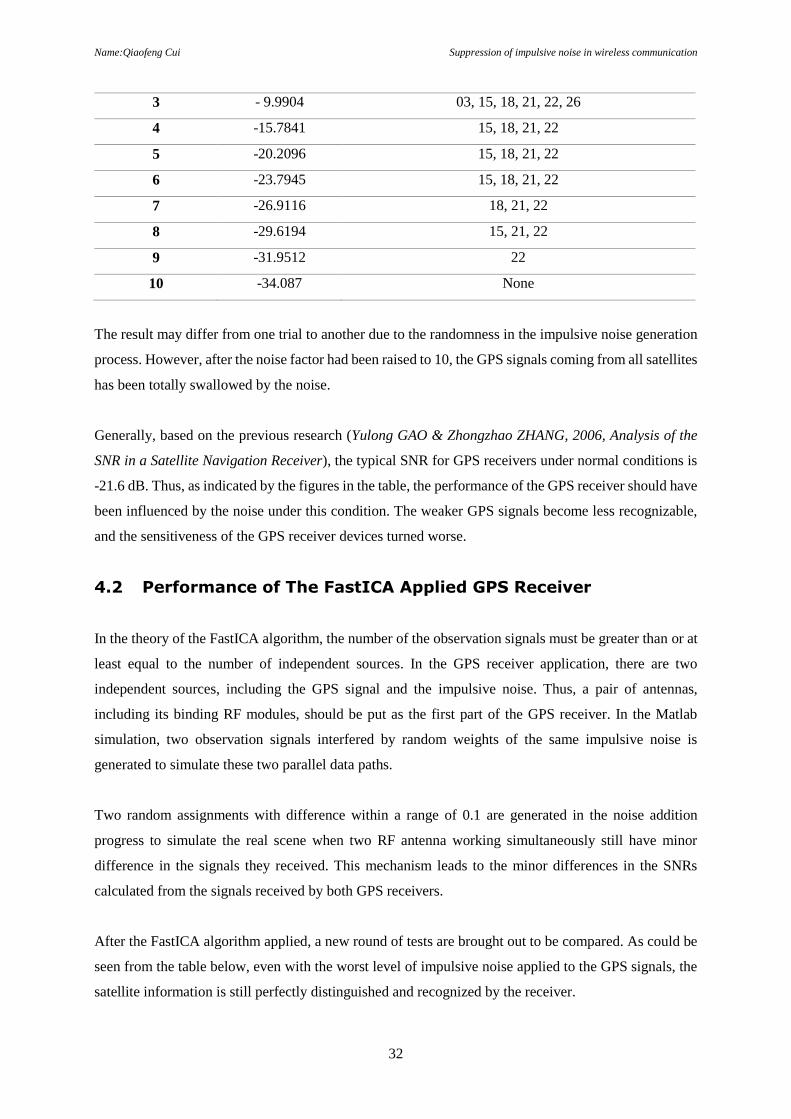
32

3 - 9.9904 03, 15, 18, 21, 22, 26

4 -15.7841 15, 18, 21, 22

5 -20.2096 15, 18, 21, 22

6 -23.7945 15, 18, 21, 22

7 -26.9116 18, 21, 22

8 -29.6194 15, 21, 22

9 -31.9512 22

10 -34.087 None

The result may differ from one trial to another due to the randomness in the impulsive noise generation

process. However, after the noise factor had been raised to 10, the GPS signals coming from all satellites

has been totally swallowed by the noise.

Generally, based on the previous research (Yulong GAO & Zhongzhao ZHANG, 2006, Analysis of the

SNR in a Satellite Navigation Receiver), the typical SNR for GPS receivers under normal conditions is

-21.6 dB. Thus, as indicated by the figures in the table, the performance of the GPS receiver should have

been influenced by the noise under this condition. The weaker GPS signals become less recognizable,

and the sensitiveness of the GPS receiver devices turned worse.

4.2 Performance of The FastICA Applied GPS Receiver

In the theory of the FastICA algorithm, the number of the observation signals must be greater than or at

least equal to the number of independent sources. In the GPS receiver application, there are two

independent sources, including the GPS signal and the impulsive noise. Thus, a pair of antennas,

including its binding RF modules, should be put as the first part of the GPS receiver. In the Matlab

simulation, two observation signals interfered by random weights of the same impulsive noise is

generated to simulate these two parallel data paths.

Two random assignments with difference within a range of 0.1 are generated in the noise addition

progress to simulate the real scene when two RF antenna working simultaneously still have minor

difference in the signals they received. This mechanism leads to the minor differences in the SNRs

calculated from the signals received by both GPS receivers.

After the FastICA algorithm applied, a new round of tests are brought out to be compared. As could be

seen from the table below, even with the worst level of impulsive noise applied to the GPS signals, the

satellite information is still perfectly distinguished and recognized by the receiver.


33

Table. 2. The Satellites Acquisition Result After FastICA Applied

Noise Factor SNR0 (dB) SNR1(dB) Acquired Satellite Indexes

0 undefined undefined 03, 06, 09, 15, 18, 21, 22, 26

1 12.4079 11.3877 03, 06, 09, 15, 18, 21, 22, 26

2 -0.5049 -1.9202 03, 06, 09, 15, 18, 21, 22, 26

3 -10.6331 -9.1413 03, 06, 09, 15, 18, 21, 22, 26

4 -14.0420 -15.4888 03, 06, 09, 15, 18, 21, 22, 26

5 -19.5934 -20.6150 03, 06, 09, 15, 18, 21, 22, 26

6 -22.2545 -22.9133 03, 06, 09, 15, 18, 21, 22, 26

7 -27.2590 -26.2262 03, 06, 09, 15, 18, 21, 22, 26

8 -31.1870 -30.0150 03, 06, 09, 15, 18, 21, 22, 26

9 -32.0064 -31.8216 03, 06, 09, 15, 18, 21, 22, 26

10 -34.1920 -34.8607 03, 06, 09, 15, 18, 21, 22, 26

To observe the impact of the impulsive noise to the GPS signal, two figures are given below.

Figure 16: The BPSK Modulated GPS Signal Sent From the Satellites.

Figure 17: The GPS Signal Received At the Receivers on Earth

In the first waveform, the uncontaminated GPS signal is uniform and trim, whereas after the impulsive

noise is added to it, the waveform become scrambled and in mess.


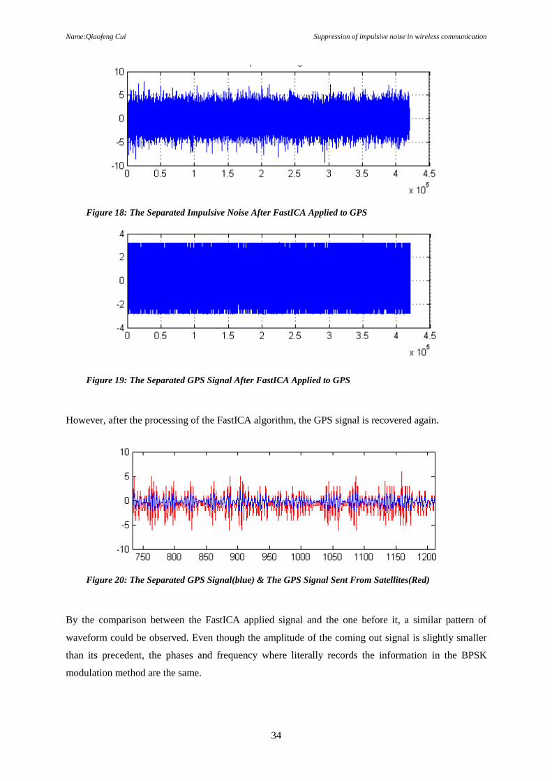
34

Figure 18: The Separated Impulsive Noise After FastICA Applied to GPS

Figure 19: The Separated GPS Signal After FastICA Applied to GPS

However, after the processing of the FastICA algorithm, the GPS signal is recovered again.

Figure 20: The Separated GPS Signal(blue) & The GPS Signal Sent From Satellites(Red)

By the comparison between the FastICA applied signal and the one before it, a similar pattern of

waveform could be observed. Even though the amplitude of the coming out signal is slightly smaller

than its precedent, the phases and frequency where literally records the information in the BPSK

modulation method are the same.


35

5 Discussion

In the description above, FastICA has been proved to be a very effective way that could be applied to

the state-of-art GPS wireless communication system to improve its preciseness and sensitivity.

However, to apply this algorithm, duplex cost must be paid. This is because that, in the theory of the

FastICA algorithm, the number of the observation signals must be larger or at least equal to the number

of the independent sources. In the case of this application, the minimum need would be two observation

signals, which require two identical RF receivers to collect.

Beyond this, duplex cost exist in the base band signal processing part as well. As in the FastICA

algorithm, which one of the separation signals is the original GPS signal is unpredictable. Thus the most

straightforward way to deal with this is to simply take trials on both. This would introduce double cost

either in the time or in the size.

Furthermore, imagine that if this algorithm is applied to other more complex communication systems,

would the result still like this perfect? The answer could not be sure until other similar researches has

been done and compared with this work.

In this thesis, FastICA has identified its advanced efficiency and infinite possibilities to solve more

complicated data processing issues. However, impulsive noise would not be the only noise source that

the industry would met when it comes to solving problems in the reality. On the other hand, more

advance wireless communication protocols had been widely used in modern wireless communication

systems, such as QPSK modulation technology, 64QAM modulation technology, or even 256QAM

modulation technology. These new rise technologies has put more question marks in front of people and

urge researches to challenge and find out.

The deduction of the FastICA algorithm has been very detailed, but the verification process still have a

lot more room to get improved. For example, besides the negentropy, other clues could be found out to

further reduce the cost during the iteration loop processing.


36

6 Conclusions

In this thesis, the FastICA algorithm has been fully verified. An application of the FastICA algorithm

on the GPS receiver is assumed and verified by MATLAB simulation. The result turned out that FastICA

is effective in eliminating the interference of the impulsive noise from the GPS receiver end. Meanwhile,

as the impulsive noise is randomly generated in the simulation process, the repeated simulation has

revealed its independency of the pattern of the noise, which is better than most of other BSS algorithm

that had been researched..

By comparing the result of the recovered signal vectors coming out from the FastICA algorithm, with

the original source signal vectors generated at the beginning, the use of FastICA in industrial impulsive

noise elimination has been functionally fully verified. The signal rehabilitated at the final end carries all

important information that the system need to recover the binary code, including the phase keying status.

The GPS signal were perfectly recovered and the satellite information carried by its features were

recognized. From this aspect, FastICA could be widely used in those industrial environments where

there are severe mechanical low frequency noises interfering digital communications.

However, due to the knowledge of the author, and the limit to this thesis, there are still a lot of work

could be done in the future to further dig into this area.

Fixed point algorithm is just one way to solve such problems, and maximum negentropy estimation also

is not the only approach to iteratively recover the original source signals. By trials of different methods

and comparing the overheads and efficiency between them could be of very considerable importance

when talking about the contribution to the digital wireless communication system researches.


37

References

[1] Jose Lago-Fernandez and John Salter, “Modeling impulsive interference in DVB-T,”

BBC Research and Development.

[2] Borre, Kai, Dennis M. Akos, Nicolaj Bertelsen, Peter Rinder, and Søren Holdt Jensen,

“A software-defined GPS and Galileo receiver: a single-frequency approach. Springer,”

2007.

[3] J.Jose, “Statistical characterization of environment at the hospital of Gävle,” master

thesis of Telecommunication 2009, Gävle, Sweden, 2009.

[4] Hyvärinen, A and Oja, E, “Independent Component Analysis: Algorithms and

Applications,” Neural Networks, Vol. 13, Issue. 4-5, pp. 411-430, 2000.

[5] Hyvärinen, A, “Fast and Robust Fixed-Point Algorithms for Independent Component

Analysis,” IEEE Transactions on Neural Networks, Vol. 10, Issue. 3, pp. 626-634, 1999.

[6] Hyävrinen, A., Karhunen, J., Oja, E.,”Independent Component Analysis,” New York:

Wiley, 2001.

[7] Kaya Y, KobayashiK, “A Basic study on Human Recognition. In Frontiers of Pattern

Recognition [M],” New York: Academic, pp. 265-289, 1971.

[8] Kanad T., “Picture processing system by computer and recognition of human face [D],”

Kyoto:Kyoto University, 1973.

[9] Manjunath B S, Chellappa R., “A feature based approach to face recognition [C],” In

IEEE Proceedings of Computer Vision and Pattern Recognition, pp. 373-378, 1992.

[10] Adini Y, Mosed Y, Ullman S., “Face recognition: The problem of compensating

for changes in illumination direction [J],” IEEE Transactions on Pattern Analysis and

Machine Intelligence, Vol. 19, Issue. 7, pp. 312-317, 1997.

[11] Laurenz Wiskott, Jean Marc Fellous, Norbert Kruger, “Face recognition by elastic

bunch graph matching [J],” IEEE Transactions on Pattern Analysis and Machine

Intelligence, Vol. 19, Issue.7, pp. 412-416, 1997.

[12] [30]Shi Zhenwei,Tang Huanwen,Liu Wenyn,and Tang Yiyuan, “Blind source

separation of more sources than mixtures using generalized exponential mixture models,”

Neurocomputing, Vol. 61, pp. 461-469, 2004.

[13] Shi Zhenwei,Tang Huanwen, and Tang Yiyuan, “A clustering approach for blind

source separation with more sources than mixtures,” Lecture Notes in Computer Science,

pp. 684-689, 2004.


38

[14] Shi Zhenwei,Tang Huanwen, and Tang Yiyuan.Sparse, “Mixture models for blind

source separation with more sources than mixtures,” Pattern Recognition Letters, 2004.

[15] A. Hyv arinen, E. Oja.A, “Fast fixed-point algorithm for independent component

analysis [J],” Neural Computation, Vol. 9, Issue. 7, pp. 1483–1492, 1997.

[16] A. Hyvärinen, “Fast and Robust Fixed-Point Algorithms for Independent

Component Analysis [J],” IEEE Transactions on Neural Networks, Vol.10, Issue. 3, pp.

626-634, 1999.

[17] Lee Te-Won, “Independent component analysis using an extended infomax

algorithm for mixed sub-Gaussian and super-Gaussian sources [J],” Neural computation,

Vol. 11, Issue. 2, pp. 409- 433, 1999.

[18] Deniz Erdogmus, Kenneth E. Hild II, Yadunandana N. Rao, Jose C., “Principal

Minimax Mutual Information Approach for Independent Component Analysis [J],”

Computational Neuro-Engineering Laboratory, University of Florida, Gainesville, FL

32611, USA .2002.

[19] A. Hyv arinen, “Denoising of sensory data by maximum likelihood estimation of

sparse components[C],” In Proc. Int. Conf. on Artificial Neural Networks, Vol. 141–

146, 1998, Sk ovde, Sweden.

[20] Turk M. and Pentland A., “Eigenfaces for Recognition [J],” Journal of Cognitive

Neurosience, Vol. 3, Issue. 1, 1995.

[21] Phillips P J , Moon H,Rauss P J Rizvis, “The FERET evaluation methodology for

face rebognition algorithms,” IEEE Trans.PAMI., Vol. 22, Issue 10, pp. 1090-1104,

2000.

[22] Vladimir N. Vapnik, “An overview of Statistical Learning Theory [J],” IEEE

Transactions on Neural Networks, pp. 988-999, 1999.

[23] Bemhard Scholkopf, Alexander J. Smola, “Learning with Kernels [M],” Britain,

The MIT Press, pp. 45-48, 2001.

[24] Liyu Liu and Amin, M.G., “Performance Analysis of GPS Receivers in Non-

Gaussian Noise Incorporating Precorrelation Filter and Sampling Rate Signal

Processing,” IEEE Transactions on Neural Networks, Vol.56, Issue.3, pp. 990-1004,

March 2008.

[25] W. Zhuang and J. Tranquilla, “Modeling and analysis for the GPS pseudo-range

observable,” IEEE Trans. Aerosp. Electron. Syst., Vol. 31, Issue. 2, pp.739 -751, 1995

[26] M. S. Braasch, “Autocorrelation sidelobe consideration in the characterization of

multipath errors,” IEEE Trans. Aerosp. Electron. Syst., Vol. 33, Issue. 1, pp.290 -295,


39

1997.

[27] R. L. Fante and J. J. Vaccaro “Evaluation and reduction of multipath-induced bias

on GPS time-of-arrival,” IEEE Trans. Aerosp. Electron. Syst., Vol. 39, Issue. 3, pp.911

-920, 2003.

[28] J. W. Erickson , P. S. Maybeck and J. F. Raquet “Multipath-adaptive GPS/INS

receiver,” IEEE Trans. Aerosp. Electron. Syst., Vol. 41, Issue. 2, pp.645 -657, 2005.

[29] J. Soubielle, I. Fijalkow, P. Duvaut and A. Bibaut “GPS positioning in a multipath

environment,” IEEE Trans. Signal Process. Vol. 50, Issue. 1, pp.141 -150, 2002.

[30] M. G. Amin , L. Zhao and A. R. Lindsey “Subspace array processing for the

suppression of FM jamming in GPS receivers”, IEEE Trans. Aerosp. Electron. Syst.,

Vol. 40, Issue. 1, pp.80 -92, 2004.

[31] M. G. Amin and W. Sun “A novel interference suppression scheme for global

navigation satellite systems using antenna array”, IEEE J. Sel. Areas Commun., Vol. 23,

Issue. 5, pp.999 -1012, 2005.

[32] P. H. Mdhani, P. Axelrad, K. Krumvieda and J. Thomas “Application of

successive interference cancellation to the GPS pseudolite near-far problem”, IEEE

Trans. Aerosp. Electron. Syst., Vol. 39, Issue. 2, pp. 481 -488, 2003.

[33] O. L. Frost “An algorithm for linearly constrained adaptive array processing”,

Proc. IEEE, Vol. 60, Issue. 8, pp. 926 -935, 1972.

[34] M. Trinkle and W. Cheuk, “Null-steering GPS dual-polarised antenna arrays,”

Satellite Navigation Technology Including Mobile Positioning Location Services, 2003.


C1

Appendix A

%%%%%% GENERATE BPSK SIGNAL %%%%%% clear all; clc; close all; N=100; src_sig = randint(N,1,2,0); %generate source vector freq_carrier=10000; T=0:2*pi/99:2*pi; carrier_sig=sin(freq_carrier*T);%generate the carrier phase_ext=[]; carrier_ext=[]; for n=1:length(src_sig); %generate the keying vector if src_sig(n)==0; %bin=0, phase switch to -90 phase_shift=-ones(1,100); else src_sig(n)==1; %bin=1, phase switch to 90 phase_shift=ones(1,100); end phase_ext=[phase_ext phase_shift]; carrier_ext=[carrier_ext carrier_sig]; end bpsk_sig(1,:)=phase_ext.*carrier_ext; %generate BPSK signal

%%%%%%% PLOT THE BPSK SIGNAL %%%%%% figure(1) subplot(3,1,1);plot(bpsk_sig(1,:),'LineWidth',1);grid on; title('BPSK

Signal'); axis([0 100*length(src_sig) -2.5 2.5]);

%%%%%%% GENERATE THE NOISE %%%%%%% in_sig0=(rand(1,length(bpsk_sig(1,:)))<.5)*2-1; in_sig1=log(rand(1,length(bpsk_sig(1,:)))); impul_noise_sig=in_sig0.*in_sig1;

%%%%%%% GENERATE ONE MIXED SIGNAL %%%%%% obs_sig=bpsk_sig(1,:)+impul_noise_sig(1,:);

%%%%%%% PLOT THE SIGNALS %%%%%% subplot(3,1,2);plot(impul_noise_sig(1,:),'LineWidth',1);grid

on;title('Impulsive Noise'); subplot(3,1,3);plot(obs_sig,'LineWidth',1);grid on;title('Observation

Signal');

%%%%%% GENERATE TWO OBSERVATION SIGNALS MIXED WITH RANDOM WEIGHINGS %%%%%% rand_assig_1=rand(1,2); rand_assig_2=rand(1,2); obs_sigs(1,:)=(rand_assig_1*[obs_sig;impul_noise_sig]); obs_sigs(2,:)=(rand_assig_2*[obs_sig;impul_noise_sig]);

%%%%%% PLOT BOTH OBSERVATION SIGNALS %%%%%% figure(2) subplot(2,1,1);plot(obs_sigs(1,:),'LineWidth',1);grid on;title('1st

observation signal mixed with random weighing 1'); subplot(2,1,2);plot(obs_sigs(2,:),'LineWidth',1);grid on;title('2nd

observation signal mixed with random weighing 2');


C2

%%%%%% ICA CALCULATION %%%%%% %%%%%% centralization processing %%%%%% meanValue=mean(obs_sigs')'; cntrlzed_sig =zeros(size(obs_sigs)); cntrlzed_sig=obs_sigs-meanValue*ones(1,size(obs_sigs,2)); %%%%%% whitening processing %%%%%% covarianceMatrix = cov(cntrlzed_sig', 1); [E, D] = eig(covarianceMatrix); whitening_matrix=inv(sqrt(D))*(E)'; white_sig= whitening_matrix *cntrlzed_sig; %%%%%% initialization %%%%%% [m,samplenum]=size(white_sig); B=zeros(m);%initialize B, B=[b1;b2;……;bd] max_iteration = 100;%set the maximum iteration times %%%%%% iteration loop %%%%%% for p=1:m i=1; b = 2*(rand(m,1)-.5);%set b to random b = b/norm(b);%normalize b while i <= max_iteration bold = b;%initialize b u = 1; t = white_sig'*b; g = t.^3; dg = 3*t.^2; b = ((1-u)*t'*g*b+u*white_sig*g)/samplenum-mean(dg)*b;%core

equation b = b-B'*B*b;%orthogonalization b = b/norm(b); if abs(abs(b'*bold)-1) < 1e-9 %if b is converge B(p,:) = b;%save the vector b break; end i = i + 1; end end ica=B*whitening_matrix*obs_sigs;

%%%%%% PLOT THE ICA PROCESSED SIGNALS %%%%%% figure(3) subplot(2,1,1);plot(ica(1,:),'LineWidth',1);grid on; title('Separation Singal 1'); ylabel('y1'); subplot(2,1,2);plot(ica(2,:),'LineWidth',1);grid on; title('Separation Singal 2'); ylabel('y2');

%%%%%% PLOT COMPARISON BETWEEN 2 SEPARATION SIGNALS %%%%%% figure(4) subplot(2,1,1);plot(impul_noise_sig(1,:),'r');hold on;plot(ica(2,:),'b'); title('Separation Signal 2 with Impulsive Noise(in red)'); subplot(2,1,2);plot(bpsk_sig(1,:),'r');hold on;plot(ica(1,:),'b'); title('Separation Signal 1 with BPSK Signal(in red)'); %red line is souce signal


C3

Appendix B

@ postProcessing.m

%% Impulsive Noise Applied ================================================ noise_factor = 10; noise_sig = noise_generator(data, noise_factor); [obs_sig(1,:),SNR] = add_noise(data, noise_sig); disp(['1st impulsive noise added, SNR is ', num2str(SNR),'dB']); [obs_sig(2,:),SNR] = add_noise(data, noise_sig); disp(['2nd impulsive noise added, SNR is ', num2str(SNR),'dB']); ica = fastICA(obs_sig); data = -ica(2,:);

@ fastICA.m

function ica_sig = fastICA(obs_sigs) %%%%%% ICA CALCULATION %%%%%% %%%%%% centralization processing %%%%%% meanValue=mean(obs_sigs')'; cntrlzed_sig =zeros(size(obs_sigs)); cntrlzed_sig=obs_sigs-meanValue*ones(1,size(obs_sigs,2)); %%%%%% whitening processing %%%%%% covarianceMatrix = cov(cntrlzed_sig', 1); [E, D] = eig(covarianceMatrix); whitening_matrix=inv(sqrt(D))*(E)'; white_sig= whitening_matrix *cntrlzed_sig; %%%%%% initialization %%%%%% [m,samplenum]=size(white_sig); B=zeros(m);%initialize B, B=[b1;b2;……;bd] max_iteration = 100;%set the maximum iteration times %%%%%% iteration loop %%%%%% for p=1:m i=1; b = 2*(rand(m,1)-.5);%set b to random b = b/norm(b);%normalize b while i <= max_iteration bold = b;%initialize b u = 1; t = white_sig'*b; g = t.^3; dg = 3*t.^2; b = ((1-u)*t'*g*b+u*white_sig*g)/samplenum-mean(dg)*b;%core

equation b = b-B'*B*b;%orthogonalization b = b/norm(b); if abs(abs(b'*bold)-1) < 1e-9 %if b is converge B(p,:) = b;%save the vector b break; end i = i + 1; end end ica=B*whitening_matrix*obs_sigs; ica_sig=ica;

%%%%%% PLOT THE ICA PROCESSED SIGNALS %%%%%% figure(3) subplot(2,1,1);plot(ica(1,:),'LineWidth',1);grid on; title('Separation Singal 1');


C4

ylabel('y1'); subplot(2,1,2);plot(ica(2,:),'LineWidth',1);grid on; title('Separation Singal 2'); ylabel('y2');

@ add_noise.m

function [mix_sig,SNR] = add_noise(clr_sig, impul_noise_sig) %%%%%%% GENERATE ONE MIXED SIGNAL %%%%%% rand_assig=(rand(1,2)+10)./10 mix_sig=rand_assig*[clr_sig(1,:);impul_noise_sig(1,:)]; pow_sig=sum(((clr_sig(1,:)).*rand_assig(1,1)).^2); pow_noise=sum(((impul_noise_sig(1,:)).*rand_assig(1,2)).^2); SNR=10*log(pow_sig/pow_noise);

%%%%%%% PLOT THE SIGNALS %%%%%% figure subplot(3,1,2);plot(clr_sig(1,:),'LineWidth',1);grid on;title('BPSK

Signal Sent From GPS Satellites'); subplot(3,1,3);plot(mix_sig,'LineWidth',1);grid on;title('BPSK Signal

Received at GPS Receivers');

@ noise_generator.m

function impul_noise_sig = noise_generator(clr_sig, noise_factor) close all; %%%%%%% GENERATE THE NOISE %%%%%%% in_sig0=(rand(1,length(clr_sig(1,:)))<.5)*2-1; in_sig1=log(rand(1,length(clr_sig(1,:)))); impul_noise_sig=in_sig0.*in_sig1.*noise_factor;

Name:Qiaofeng Cui Septemper 2014 Master’s Thesis in ...

Documents

Transcript of Name:Qiaofeng Cui Septemper 2014 Master’s Thesis in ...