N-gram models §  Unsmoothed n-gram models (finish slides from last class) §  Smoothing

–  Add-one (Laplacian) –  Good-Turing

§  Unknown words §  Evaluating n-gram models §  Combining estimators

–  (Deleted) interpolation –  Backoff

Smoothing

§  Need better estimators than MLE for rare events

§  Approach – Somewhat decrease the probability of

previously seen events, so that there is a little bit of probability mass left over for previously unseen events

» Smoothing » Discounting methods

Add-one smoothing §  Add one to all of the counts before normalizing

into probabilities §  MLE unigram probabilities

§  Smoothed unigram probabilities

§  Adjusted counts (unigrams)

NwcountwP x

x)()( =

VNNcc ii +

+= )1(*

VNwcountwP x

x +

+=

1)()(

corpus length in word tokens

vocab size (# word types)

Add-one smoothing: bigrams

[example on board]

Add-one smoothing: bigrams §  MLE bigram probabilities

§  Laplacian bigram probabilities

P(wn |wn!1) =count(wn!1wn )count(wn!1)

P(wn |wn!1) =count(wn!1wn )+1count(wn!1)+V

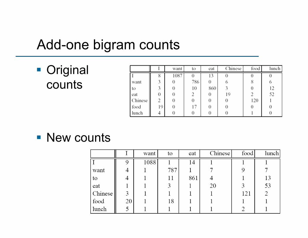
Add-one bigram counts

§  Original counts

§  New counts

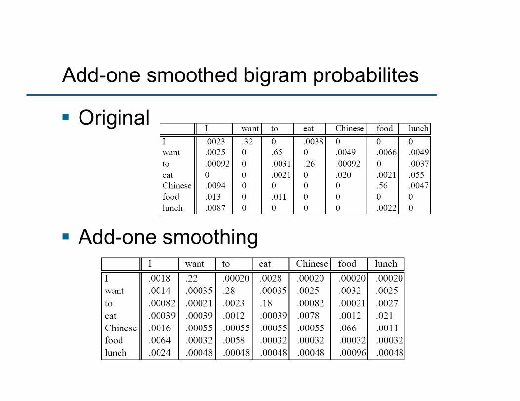
Add-one smoothed bigram probabilites

§  Original

§  Add-one smoothing

Too much probability mass is moved!

Too much probability mass is moved

§  Estimated bigram frequencies

§  AP data, 44 million words –  Church and Gale (1991)

§  In general, add-one smoothing is a poor method of smoothing

§  Often much worse than other methods in predicting the actual probability for unseen bigrams

r = fMLE femp fadd-1

0 0.000027 0.000137

1 0.448 0.000274

2 1.25 0.000411

3 2.24 0.000548

4 3.23 0.000685

5 4.21 0.000822

6 5.23 0.000959

7 6.21 0.00109

8 7.21 0.00123

9 8.26 0.00137

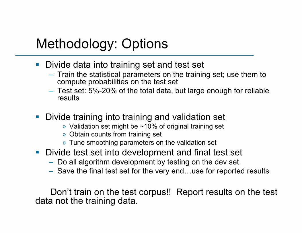
Methodology: Options §  Divide data into training set and test set

–  Train the statistical parameters on the training set; use them to compute probabilities on the test set

–  Test set: 5%-20% of the total data, but large enough for reliable results

§  Divide training into training and validation set

»  Validation set might be ~10% of original training set »  Obtain counts from training set »  Tune smoothing parameters on the validation set

§  Divide test set into development and final test set –  Do all algorithm development by testing on the dev set –  Save the final test set for the very end…use for reported results

Don’t train on the test corpus!! Report results on the test data not the training data.

Good-Turing discounting

§  Re-estimates the amount of probability mass to assign to N-grams with zero or low counts by looking at the number of N-grams with higher counts.

§  Let Nc be the number of N-grams that occur c times. –  For bigrams, N0 is the number of bigrams of count 0,

N1 is the number of bigrams with count 1, etc. §  Revised counts:

c

c

NNcc 1* )1( ++=

Good-Turing discounting results §  Works very well in

practice §  Usually, the GT

discounted estimate c* is used only for unreliable counts (e.g. < 5)

§  As with other discounting methods, it is the norm to treat N-grams with low counts (e.g. counts of 1) as if the count was 0

r = fMLE femp fadd-1 fGT

0 0.000027 0.000137 0.000027

1 0.448 0.000274 0.446

2 1.25 0.000411 1.26

3 2.24 0.000548 2.24

4 3.23 0.000685 3.24

5 4.21 0.000822 4.22

6 5.23 0.000959 5.19

7 6.21 0.00109 6.21

8 7.21 0.00123 7.24

9 8.26 0.00137 8.25

N-gram models §  Unsmoothed n-gram models (review) §  Smoothing

–  Add-one (Laplacian) –  Good-Turing

§  Unknown words §  Evaluating n-gram models §  Combining estimators

–  (Deleted) interpolation –  Backoff

Unknown words

§  Closed vocabulary – Vocabulary is known in advance – Test set will contain only these words

§  Open vocabulary – Unknown, out of vocabulary words can occur – Add a pseudo-word <UNK>

§  Training the unknown word model???

Evaluating n-gram models §  Best way: extrinsic evaluation

–  Embed in an application and measure the total performance of the application

–  End-to-end evaluation §  Intrinsic evaluation

–  Measure quality of the model independent of any application

–  Perplexity »  Intuition: the better model is the one that has a tighter fit to the

test data or that better predicts the test data

Perplexity

For a test set W = w1 w2 … wN, PP (W) = P (w1 w2 … wN)

-1/N

The higher the (estimated) probability of the word sequence, the lower the perplexity.

Must be computed with models that have no knowledge of the test set.

=1

P(w1w2...wN )N

N-gram models §  Unsmoothed n-gram models (review) §  Smoothing

–  Add-one (Laplacian) –  Good-Turing

§  Unknown words §  Evaluating n-gram models §  Combining estimators

–  (Deleted) interpolation –  Backoff

Combining estimators §  Smoothing methods

–  Provide the same estimate for all unseen (or rare) n-grams with the same prefix

–  Make use only of the raw frequency of an n-gram §  But there is an additional source of knowledge we can

draw on --- the n-gram “hierarchy” –  If there are no examples of a particular trigram,wn-2wn-1wn, to

compute P(wn|wn-2wn-1), we can estimate its probability by using the bigram probability P(wn|wn-1 ).

–  If there are no examples of the bigram to compute P(wn|wn-1), we can use the unigram probability P(wn).

§  For n-gram models, suitably combining various models of different orders is the secret to success.

Simple linear interpolation

§  Construct a linear combination of the multiple probability estimates. –  Weight each contribution so that the result is

another probability function.

–  Lambda’s sum to 1.

§  Also known as (finite) mixture models §  Deleted interpolation

–  Each lambda is a function of the most discriminating context

)()|()|()|( 11212312 nnnnnnnnn wPwwPwwwPwwwP λλλ ++= −−−−−

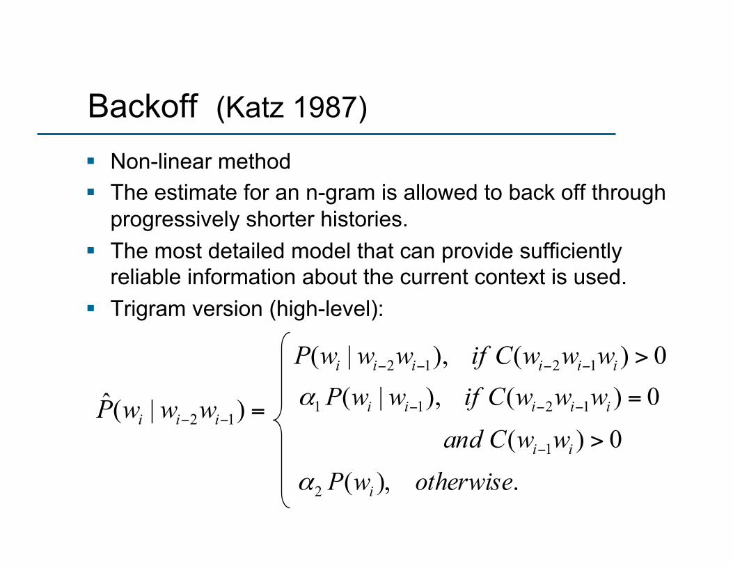
Backoff (Katz 1987)

§  Non-linear method §  The estimate for an n-gram is allowed to back off through

progressively shorter histories. §  The most detailed model that can provide sufficiently

reliable information about the current context is used. §  Trigram version (high-level):

=−− )|(ˆ 12 iii wwwP

0)(),|( 1212 >−−−− iiiiii wwwCifwwwP

0)(

0)(),|(

1

1211

>

=

−

−−−

ii

iiiii

wwCandwwwCifwwPα

.),(2 otherwisewP iα

Final words… §  Problems with backoff?

–  Probability estimates can change suddenly on adding more data when the back-off algorithm selects a different order of n-gram model on which to base the estimate.

–  Works well in practice in combination with smoothing.

§  Good option: simple linear interpolation with MLE n-gram estimates plus some allowance for unseen words (e.g. Good-Turing discounting)