N. E. BARAN C. C. KISIEL L. DUCKSTEIN...

A Stochastic Analysis of Flows on Rillitto Creek

Item Type text; Proceedings

Authors Baran, N. E.; Kisiel, C. C.; Duckstein, L.

Publisher Arizona-Nevada Academy of Science

Journal Hydrology and Water Resources in Arizona and the Southwest

Rights Copyright ©, where appropriate, is held by the author.

Download date 10/05/2018 08:01:05

Link to Item http://hdl.handle.net/10150/300117

http://hdl.handle.net/10150/300117

A STOCHASTIC ANALYSIS OF FLOWS ON RILLITO CREEK

N. E. BARAN

Hydrology & Water Resources, University of Arizona

C. C. KISIEL

Hydrology & Water Resources, University of Arizona

L. DUCKSTEIN

Systems Engineering, University of Arizona

INTRODUCTION

Measurements of the ephemeral streamflow of Rillito Creek, Ttcson, Arizona,

were analyzed for the period 1933 through 1965. The purpose of the analysis was

twofold: (1) to construct a simulation model for ephemeral streamflow, and

(2) to examine in depth the problem of the worth of data for that model.

The simulation model was based on the following hypotheses:

1. The durations of flows and their preceding or succeeding dry periods (periods

of time when no flow is present) are independent.

2. The distribution of the lengths of the dry periods and flows is stationary

over a certain period of the year (say, July 1 to Sept. 15).

3. A stationary probability distribution for the duration of the flows and a

stationary distribution for the length of the dry periods can be derived.

4. In this manner one can simulate a series of flows and dry periods correspond-

ing to the one in nature.

171

A corresponding problem was how to derive a simulation model for the total

amount of flow (in acre -feet) within one flow period. For this purpose three

variables were considered:

(1) the duration of the flow,

(2) the peak intensity of the flow, and

(3) the length of the dry period preceding the flow (the antecedent

dry period).

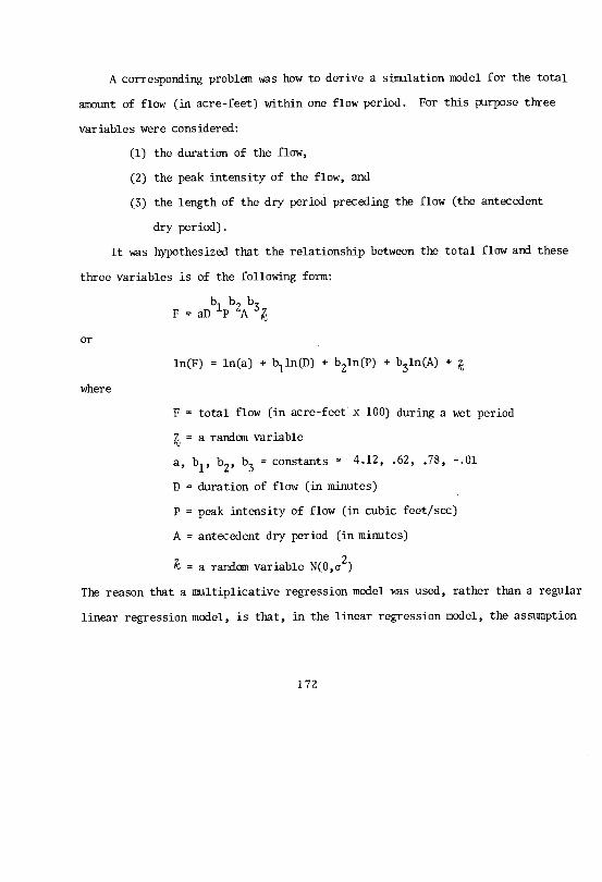
It was hypothesized that the relationship between the total flow and these

three variables is of the following form:

or

where

F = aDb1Pb2A 3Z

ln(F) = ln(a) + biln(D) + b21n(P) + b31n(A) + k

F = total flow (in acre- feet' x 100) during a wet period

= a random variable

a, bl, b2, b3 = constants . 4.12, .62, .78, -.01

D = duration of flow (in minutes)

P = peak intensity of flow (in cubic feet /sec)

A = antecedent dry period (in minutes)

k = a random variable N(0,a2)

The reason that a multiplicative regression model was used, rather than a regular

linear regression model, is that, in the linear regression model, the assumption

172

of constancy of variance does not hold since the variance increases as the three

regression variables increase. From the data, the multiple correlations R for

both summer and winter flows were on the order of 0.95, the correlation between

"independent" variables ranged from 0.04 to 0.49 which implies a form of inde-

pendence, and the residuals ti were distributed normally about the regression

hyperplane.

The regression model can be used for the two purposes mentioned above:

to predict the total amount of flow during a flow period, and to examine the worth

of data as applied to the regression analysis.

For the purpose of simulating streamflow the following algorithm can be

used:

1. Monte -Carlo a dry period and record the length of the dry period.

2. Monte -Carlo a flów duration and record the flow duration.

3. Monte -Carlo a peak flow intensity.

4. Predict an expected total flow from 1, 2, and 3.

5. Monte -Carlo a deviation from the mean total flow.

a. Add the predicted total mean flow and the deviation.

b. Record the resulting predicted total flow.

6. Go to step 1.

This algorithm is repeated for as many times as is necessary to predict a sequence

of flows.

The following sections will examine problems related to the above -mentioned

goals.

173

AN ANALYSIS OF THE WORTH OF DATA BY ANALYSIS OF VARIANCERELATIONS BETWEEN CUMULATIVE MULTIPLE LINEAR REGRESSIONS

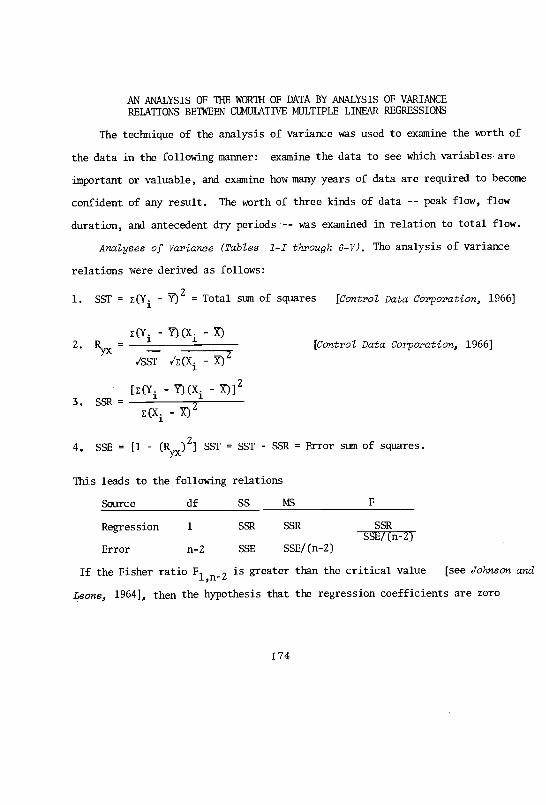
The technique of the analysis of variance was used to examine the worth of

the data in the following manner: examine the data to see which variables are

important or valuable, and examine how many years of data are required to become

confident of any result. The worth of three kinds of data -- peak flow, flow

duration, and antecedent dry periods -- was examined in relation to total flow.

Analyses of Variance (Tables 1 -I through 6 -V). The analysis of variance

relations were derived as follows:

1. SST = E(Yi - Y)2 = Total sum of squares [Control Data Corporation, 1966]

E(Y - 7) (X.

2 R - 1 1 [Control Data Corporation, 1966]

1/SST E(X - 3)2

3. SSR -[E(Yi - ?)(Xi - 7)]2

7)2

4. SSE _ [1 - (Ryx)2] SST = SST - SSR = Error sum of squares.

This leads to the following relations

Source df SS MS F

Regression 1 SSR SSR SSR

Error n -2 SSE SSE /(n -2)

SSE! (n -2)

If the Fisher ratio Fl,n_2 is greater than the critical value [see Johnson and

Leone, 1964], then the hypothesis that the regression coefficients are zero

174

cannot be rejected. Subtable I of Tables 1 through 6 presents analyses of this

type for Flow -Peak, Flow- Duration, and Flow- Antecedent Dry Period (ADP) relations.

The analysis of variance tables are numbered 1 -I through 6 -V. The first

number is the table number and stands for the time period of the analysis; the

second number (the Roman numeral) stands for the type of analysis. Therefore,

for example, Table 4 -IV presents the fourth time period (1933 through 1942) and

the fourth type of analysis (the significance of adding two variables to a re-

gression already containing one variable).

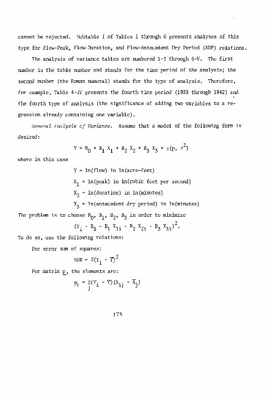
General Analysis of Variance. Assume that a model of the following form is

desired:

Y = BO + Bl X1 + B2 X2 + B3 X3 + e (p , Q2)

where in this case

Y = ln(flow) in ln(acre -feet)

X1 = ln(peak) in ln(cubic feet per second)

X2 = ln(duration) in ln(minutes)

X3 = ln(antecedent dry period) in ln(minutes)

The problem is to choose B0, B1, B2, B3 in order to minimize

(Yi - Bo - B1 Xli - B2 X2i - B3 X3i)2

To do so, use the following relations:

For error sum of squares:

SSE = E(Yi Y-)2

For matrix p, the elements are:

pi = E(Yi - 7) (Xij - X' )

175

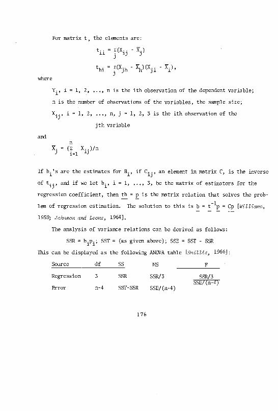
For matrix t, the elements are:

t.= E (Xij -

thi = E(Xjh - Xh) (Xj i - Xi)

where

Yi, = 1, 2, ..., n is the ith observation of the dependent variable;

n is the number of observations of the variables, the sample size;

Xij, i = 1, 2, ..., n, j = 1, 2, 3 is the ith observation of the

jth variable

andn

X. = (E X..)/n3 i=1 3

If b.'s are the estimates for Bi, if C.., an element in matrix C, is the inverse13

of tij, and if we let bi, i = 1, ..., 3, be the matrix of estimators for the

regression coefficient, then tb = p is the matrix relation that solves the prob-

lem of regression estimation. The solution to this is b = t -lp = Cp [Williams,

1959; Johnson and Leone, 1964].

The analysis of variance relations can be derived as follows:

SSR = bipi; SST = (as given above); SSE = SST - SSR

This can be displayed as the following ANOVA table [Smillie, 19661:

Source df SS MS F

Regression 3 SSR SSR /3 SSR /3

SSE /(n -4)

Error n -4 SST -SSR SSE /(n -4)

176

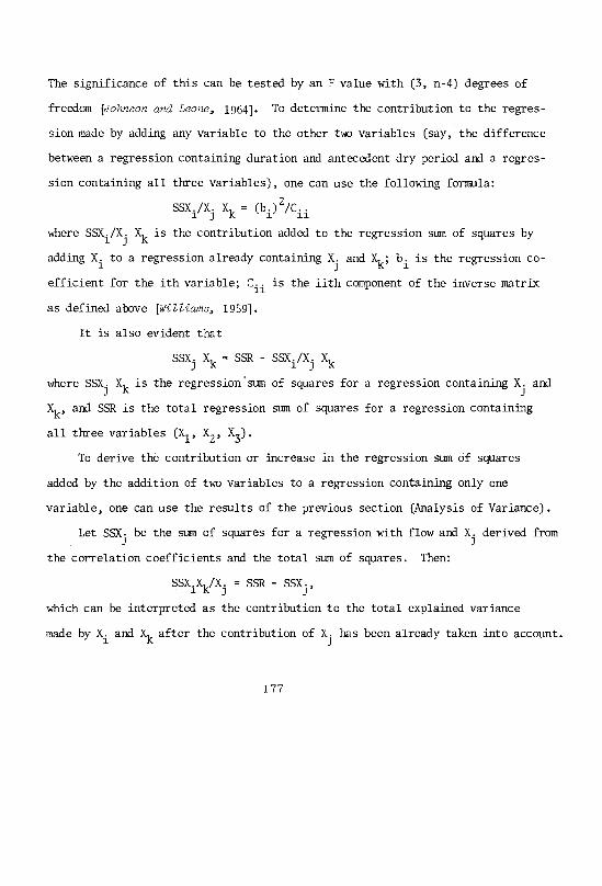
The significance of this can be tested by an F value with (3, n -4) degrees of

freedom [Johnson and Leone, 1964]. To determine the contribution to the regres-

sion made by adding any variable to the other two variables (say, the difference

between a regression containing duration and antecedent dry period and a regres-

sion containing all three variables), one can use the following formula:

SSXi /Xj Xk =

(bi)2

/iii

where SSXi /X. Xk is the contribution added to the regression sum of squares by

adding Xi to a regression already containing Xi and Xk; bi is the regression co-

efficient for the ith variable; C.. is the iith component of the inverse matrix

as defined above [Williams, 1959].

It is also evident that

SSX Xk = SSR - SSXi /X Xk

where SSXi Xk is the regressionsum of squares for a regression containing X and

Xk, and SSR is the total regression sum of squares for a regression containing

all three variables (X1, X2, X3).

To derive the contribution or increase in the regression sum of squares

added by the addition of two variables to a regression containing only one

variable, one can use the results of the previous section (Analysis of Variance).

Let SSX.3 be the sum of squares for a regression with flow and Xi derived from

the correlation coefficients and the total sum of squares. Then:

SSXiXk/Xi = SSR - SSXi,

which can be interpreted as the contribution to the total explained variance

made by Xi and Xk after the contribution of X has been already taken into account.

177

We can now derive any of the regression relations from the correlation matrix,

the total sum of squares, the total regression sum of squares, the estimated regres-

sion coefficients and the inverse matrix. Tests for the significance of the con-

tribution of sets of variables to a regression are as follows: let SSR be the

regression sum of squares for p variables, and let SSR' be the regression sum of

squares for k variables with k < p. If n sets of observations were taken, then

F SSE /(n -p -1

(SSR - SSR')/(

tests the significance of the variables not included in the regression for the

first k variables but included in the total regression [Smillie, 1966). An analy-

sis of variance table can be made for this as follows:

Source df SS MS F

All p variables p SSR

First k variables k SSR'

Difference dueto the addedvariables p - k SSR - SSR' MSR' - (SSR SSR') MSR'

p - k SI-

Error n -p -1 SSE MSE = SSE

n-p-T

In our problem we wish to evaluate:

1. the significance of each pair of variables (Tables 1 through 6, subtable

II in each Table),

2. the significance of adding each variable to a regression containing the other

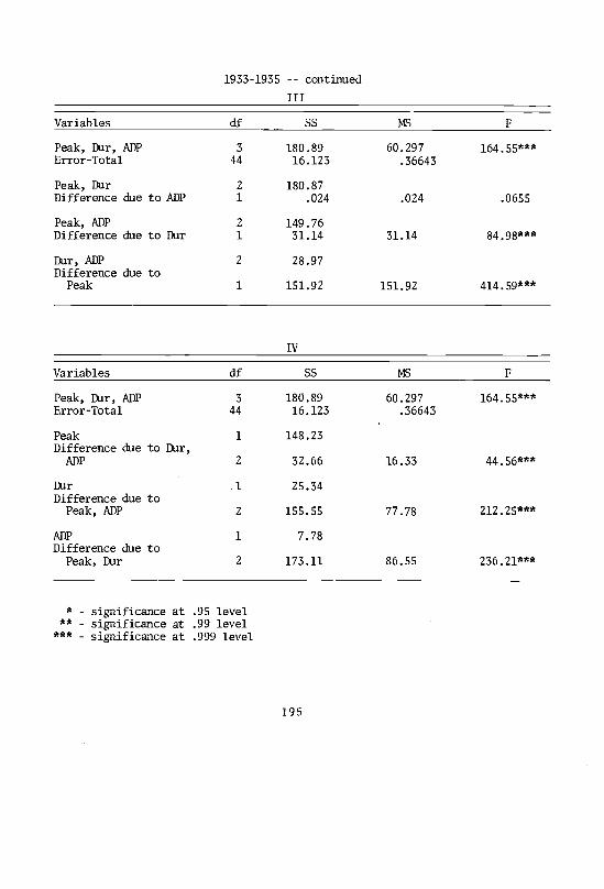
two variables (Tables 1 through 6, subtable III in each Table),

178

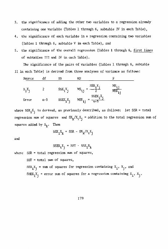
3. the significance of adding the other two variables to a regression already

containing one variable (Tables 1 through 6, subtable IV in each Table),

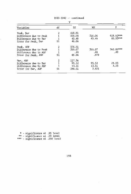
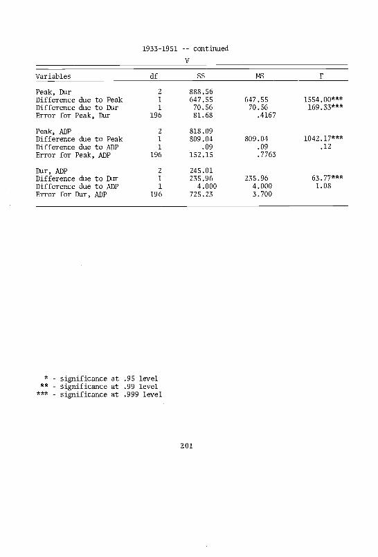
4. the significance of each variable in a regression containing two variables

(Tables 1 through 6, subtable V in each Table), and

5. the significance of the overall regression (Tables 1 through 6, first lines

of subtables III and IV in each Table).

The significance of the pairs of variables (Tables 1 through 6, subtable

II in each Table) is derived from three analyses of variance as follows:

Source df SS MS

SSX.X.

X.X.1J 2 SSX.X.1J MS.. -13

1 32

SSEX.X.

Error n-3 SSEXiXj MSEij3

n-31

F

where SSX.XJ is derived, as previously described, as follows: let SSR = total

regression sum of squares and SXk/XiXj = addition to the total regression sum of

squares added by Xk. Then

SSXiXk = SSR - SXk/XiXj

and

SSEX.X. = SST - SSX.X

where SSR = total regression sum of squares,

SST = total sum of squares,

SSX.X. = sum of squares for regression containing Xi, X., and

SSEX.X. = error sum of squares for a regression containing Xi, X.

179

The significance of these regressions containing two variables can be summarized

as follows:

1. A regression containing peak and duration is very highly significant even with

the smallest sample.

2. A regression containing peak and ADP is significant but not as good as the

above.

3. A regression containing ADP and duration becomes very highly significant at the

.999 level after 10 years, but this relationship cannot be properly evaluated

without 10 years of data.

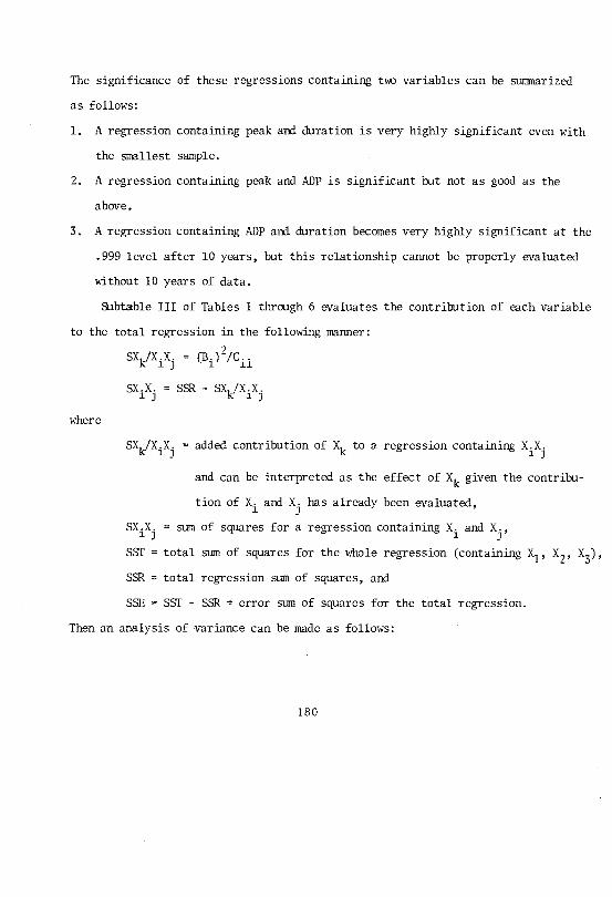
Subtable III of Tables 1 through 6 evaluates the contribution of each variable

to the total regression in the following manner:

SXk /XiXj = (B.)2/C..

SXiXj = SER - SXk/X.Xj

where

SXk /XiXj = added contribution of Xk to a regression containing X.X.

and can be interpreted as the effect of Xk given the contribu-

tion of Xi and Xj has already been evaluated,

SXiXj = sum of squares for a regression containing Xi and X.,

SST = total sum of squares for the whole regression (containing X1, X2, X3),

SSR = total regression sum of squares, and

SSE = SST - SER = error sum of squares for the total regression.

Then an analysis of variance can be made as follows:

180

Source df SS MS F

X1, X2, X3 e SSR MSR = SSR /3 MSR/MSE

Total error n -4 SSE MSE = SSE /(n -4)

X., X. 2i

Difference duedue to Xk 1

SX.X.

SXk /XiX. MSk/ij

= SXk /XiXi 14S1/.ijJMSE

The third line, XiXj, is redundant and is put in only for illustration. Lines 3

and 4 are repeated to evaluate the contribution of each variable.

Here it rapidly becomes evident that the contribution due to adding ADP into

the regression is negligible. The difference due to ADP is not significant at 3

years and indeed at 33 years of data the contribution of ADP to the total regres-

sion is .4 out of 1588.8 or .025 percent of the total regression variance. It can

be concluded from this that ADP is useless as far as the total regression is con-

cerned as virtually all the variance accounted for by ADP is accounted for by a

combination of duration and peak. The conclusion to be drawn from this is that

the expense of processing data containing antecedent dry periods should be fore-

gone. The contribution of the peak, however, is very highly significant after 3

years and the contribution of duration is also very highly significant after 3

years, indicating that the contribution of these variables can be discovered with

very little data.

Subtable IV of Tables 1 through 6 further illustrates the negligible contri-

bution made by adding ADP into the regression.

Subtable V of Tables 1 through 6 is meant to evaluate the contribution of each

variable in regressions containing two variables. Since ADP has been rejected, it

181

is necessary to determine if each of the other two variables, peak and duration,

contributes significantly to the regression containing both. An analysis of var-

iance can be constructed as follows:

SSPD = sum of squares for regression containing peak and duration,

SSP /D = SSPD - SSD = contribution of peak to regression,

SSD /P = SSPD - SSP = contribution of duration to the regression, and

Error = SSEPD = SST - SSPD

= error sum of squares for regression containing peak and duration.

The analysis of variance table is as follows:

Source df SS MS F

Peak, duration 2 SSPD

Difference dueto peak 1 SSP /D MSP /D

Difference dueto duration 1 SSD /P MSP /D

Error n-3 SSEDP MSEPD - SSEDP-173

MSP/DMSEPD

MSP/DMSEPD

Examining the significance of duration and peak to overall regression, one

finds that the contribution of each is very highly significant at only two years,

indicating that both variables contribute to the overall regression and that their

significance becomes evident with very small amounts of data.

EVALUATION OF THE ABOVE RESULTS

The following conclusions can then be drawn from the extensive analysis of

variance:

1. ADP should not be used.

182

2. A regression containing peak and duration is significant and this significance

becomes evident from a very small amount of data.

3. Both peak and duration make a significant contribution to the overall regres-

sion. This also becomes evident with a very small amount of data.

4. The significance of peak alone is evident with minimal amounts of data.

5. The significance of duration alone becomes evident if one uses about 10

years of data.

6. All of the above conclusions could have been drawn with 10 years of data.

Therefore, as far as the significance of the variables in the regression is

concerned, more than 10 years of data is wasted expense.

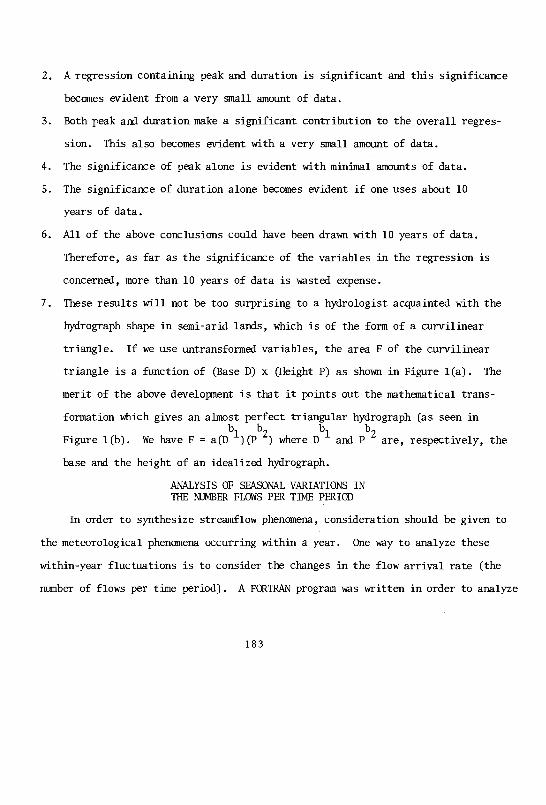
7. These results will not be too surprising to a hydrologist acquainted with the

hydrograph shape in semi -arid lands, which is of the form of a curvilinear

triangle. If we use untransformed variables, the area F of the curvilinear

triangle is a function of (Base D) x (Height P) as shown in Figure 1(a). The

merit of the above development is that it points out the mathematical trans-

formation which gives an almost perfect triangular hydrograph (as seen in

Figure 1(b). We have F = a(Db1 )(Pb2) where Dbl and Pb2 are, respectively, the

base and the height of an idealized hydrograph.

ANALYSIS OF SEASONAL VARIATIONS INTHE NUMBER FLOWS PER TINE PERIOD

In order to synthesize streamflow phenomena, consideration should be given to

the meteorological phenomena occurring within a year. One way to analyze these

within -year fluctuations is to consider the changes in the flow arrival rate (the

number of flows per time period). A FORTRAN program was written in order to analyze

183

streamflows for any arbitrary time periods within the year. Data from the Rillito

Creek from 1930 through 1965 were used for this analysis. One output from the pro-

gram was the number of flows in each time period (say, the month of July, for

example) for each of the 36 years. These flow arrivals proved most amenable to

analysis in determining "seasonal" fluctuations in streamflow.

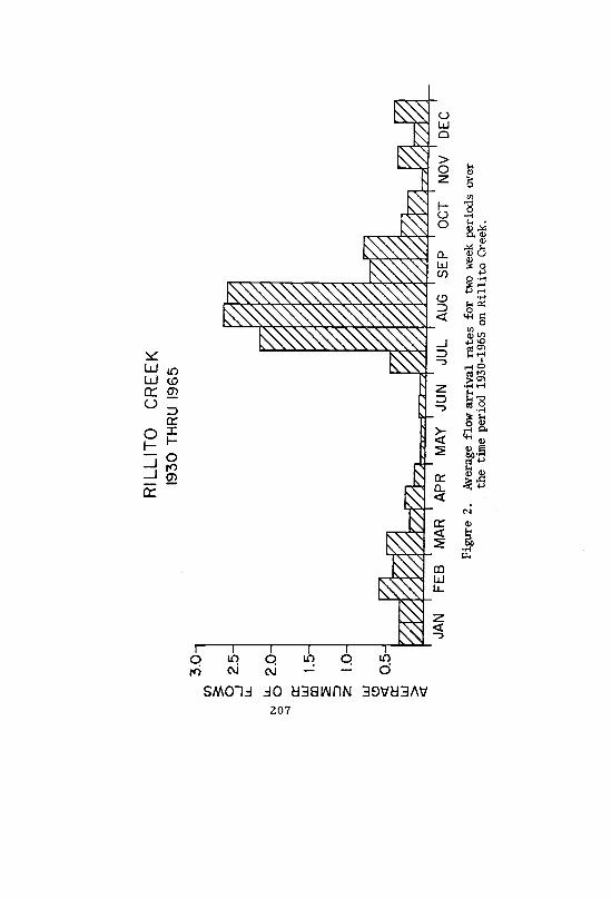
The flows were tabulated for each "two week" period throughout the year. A

"two week" period consists of days 1 through 15 of a month or days 16 through the

end of the month. The simplest statistic that one can use to analyze seasonal var-

iations is the flow arrival rate for each two week period. These appear in Figure

2, which shows, for example, that the last half of July and the month of August

seen to have significantly higher arrival rates than the rest of the year; this

hypothesis can be tested statistically.

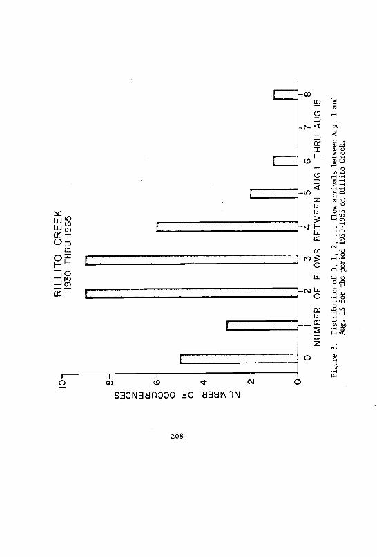
The distribution of arrivals was tabulated for each two -week period (see

Figure 2 for August 1 -15 as an example). In order to evaluate whether or not the

flow arrivals were the same in consecutive two -week periods a Kolmogorov- Smirnov

test was used. The test statistic for Kolmogorov- Smirnov test for the comparison

of two distributions is,

D = max 1F1(x) - F2(x)1

where Fi(x) is the cumulative observed probability for the ith variable.

If there are n1 observations of variable 1 and n2 observations of variable 2,

then in order to test the hypothesis, H0: F1(x) = F2(x) at the .05 significance

level, compute,

d = 1.36nl + n2

n1n2

184

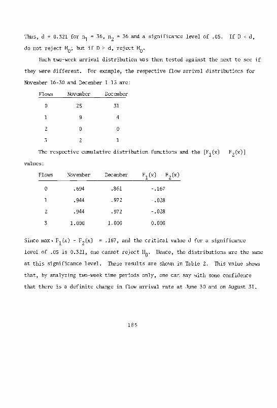
Thus, d = 0.321 for n1 = 36, n2 = 36 and a significance level of .05. If D < d,

do not reject H0; but if D > d, reject H0.

Each two -week arrival distribution was then tested against the next to see if

they were different. For example, the respective flow arrival distributions for

November 16 -30 and December 1 -15 are:

Flows November December

0 25 31

1 9 4

2 0 0

3 2 1

The respective cumulative distribution functions and the [F1(x) - F2(x)]

values:

Flows November December F1(x) - F2(x)

0 .694 .861 -.167

1 .944 .972 -.028

2 .944 .972 -.028

3 1.000 1.000 0.000

Since max. F1(x) - F2(x) = .167, and the critical value d for a significance

level of .05 is 0.321, one cannot reject H0. Hence, the distributions are the same

at this significance level. These results are shown in Table 2. This value shows

that, by analyzing two -week time periods only, one can say with some confidence

that there is a definite change in flow arrival rate at June 30 and on August 31.

185

An examination of the arrival rates indicates that grouping the observations

would be useful. Five time periods were considered as follows:

Time Period Number of Two-week Periods

1 (October 1 - April 15) 468

2 (April 16 - June 30) 180

3 (July 1 - July 15) 36

4 (July 16 - August 31) 108

5 (September 1 - September 30) 72

The cumulative distributions for these five time periods were compared by the

Kolmogorov-Snirnov test with the preceding time periods to determine if the flow

arrivals were the same. The results were computed for a comparison of Time

Period 1 with Time Period 2 by using the following relation:

4 = max IF1(n) - F2(n)I = .174max

The critical level for n1 = 468, n2 = 180, and a = .05 is 0.119. Hence, reject

the hypothesis that the flow arrivals are the same.

lows for a = .05:

Time Periods Amax Critical value

The full results are as fol-

Result

1 and 2 .174 .119 Reject H0

2 and 3 .273 .248 Reject H0

3 and 4 .565 .261 Reject H0

4 and 5 .426 .207 Reject H0

5 and 1 .224 .172 Reject H0

These results indicate that there are five different periods per year when the

flow arrival distributions are statistically different.

186

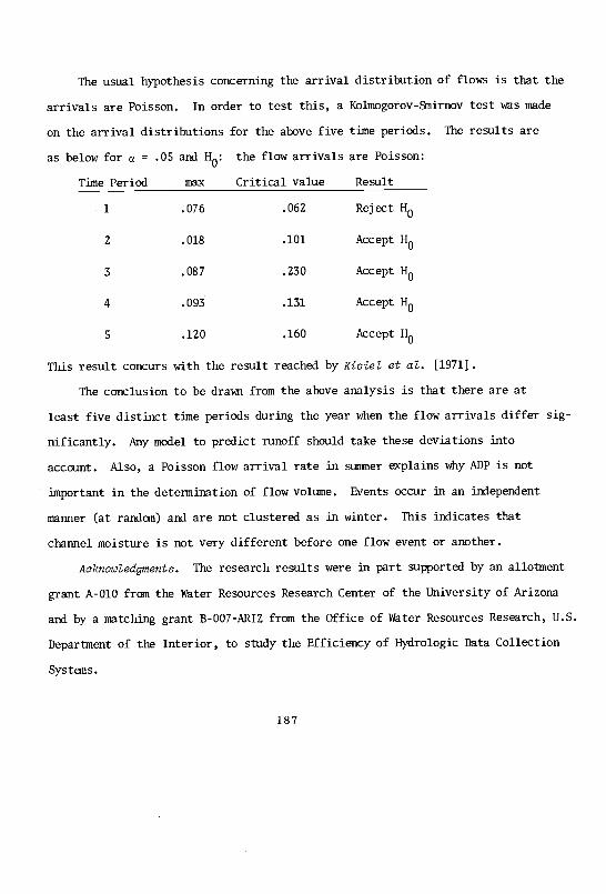
The usual hypothesis concerning the arrival distribution of flows is that the

arrivals are Poisson. In order to test this, a Kolmogorov- Smirnov test was made

on the arrival distributions for the above five time periods. The results are

as below for a = .05 and H0: the flow arrivals are Poisson:

Time Period max Critical value Result

1 .076 .062 Reject H0

2 .018 .101 Accept H0

3 .087 .230 Accept H0

4 .093 .131 Accept H0

5 .120 .160 Accept H0

This result concurs with the result reached by Kisiel et al. [1971].

The conclusion to be drawn from the above analysis is that there are at

least five distinct time periods during the year when the flow arrivals differ sig-

nificantly. Any model to predict runoff should take these deviations into

account. Also, a Poisson flow arrival rate in summer explains why ADP is not

important in the determination of flow volume. Events occur in an independent

manner (at random) and are not clustered as in winter. This indicates that

channel moisture is not very different before one flow event or another.

Acknowledgments. The research results were in part supported by an allotment

grant A -010 from the Water Resources Research Center of the University of Arizona

and by a matching grant B- 007 -ARIZ from the Office of Water Resources Research, U.S.

Department of the Interior, to study the Efficiency of Hydrologic Data Collection

Systems.

187

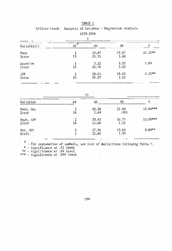
TABLE 1

Rillito Creek: Analysis of Variance - Regression Analysis

1933 -1934

I

Variable(s) df SS MS F

Peak 1 23.87 23.87 14.21 **

Error 15 25.15 1.68

Duration 1 3.32 3.32 1.09

Error 15 45.70 3.05

ADP 1 18.65 18.65 9.21 **

Error 15 30.37 2.02

II

Variables df SS MS F

Peak, Dur 2 43.38 21.69 53.84 * **

Error 14 5.64 .403

Peak, ADP 2 33.42 16.71 15.00 * **

Error 14 15.60 1.11

Dur, ADP 2 27.36 13.68 8.84 **

Error 2 21.66 1.55

- For explanation of symbols, see list of definitions following Table 7.* - significance at .95 level

** - significance at .99 level* ** - significance at .999 level

188

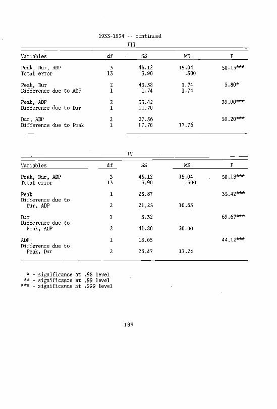
1933 -1934 -- continued

III


Peak, Dur, ADP 3 45.12 15.04 50.13 * **

Total error 13 3.90 .300

Peak, Dur 2 43.38 1.74 5.80*Difference due to ADP 1 1.74 1.74

Peak, ADP 2 33.42 39.00 * **

Difference due to Dur 1 11.70

Dur, ADP 2 27.36 59.20 * **

Difference due to Peak 1 17.76 17.76

IV


Peak, Dur, ADP 3 45.12 15.04 50.13 * **


Peak 1 23.87 35.42 * **

Difference due toDur, ADP 2 21.25 10.63

Dur 1 3.32 69.67 * **

Difference due toPeak, ADP 2 41.80 20.90

ADP 1 18.65 44.12 * **

Difference due toPeak, Dur 2 26.47 13.24

* - significance at .95 level** - significance at .99 level

* ** - significance at .999 level

189

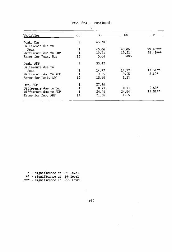
1933 -1934 -- continued

V


Peak, Dur 2 43.38

Difference due toPeak 1 40.06 40.06 99.40 * **

Difference due to Dur 1 19.51 19.51 48.41 * **

Error for Peak, Dur 14 5.64 .403

Peak, ADP 2 33.42Difference due to

Peak 1 14.77 14.77 13.31 **

Difference due to ADP 1 9.55 9.55 8.60*

Error for Peak, ADP 14 15.60 1.11

Dur, ADP 2 27.36

Difference due to Dur 1 8.71 8.71 5.62*

Difference due to ADP 1 24.04 24.04 15.51 **

Error for Dur, ADP 14 21.66 1.55

* - significance at .95 level** - significance at .99 level* ** - significance at .999 level

190

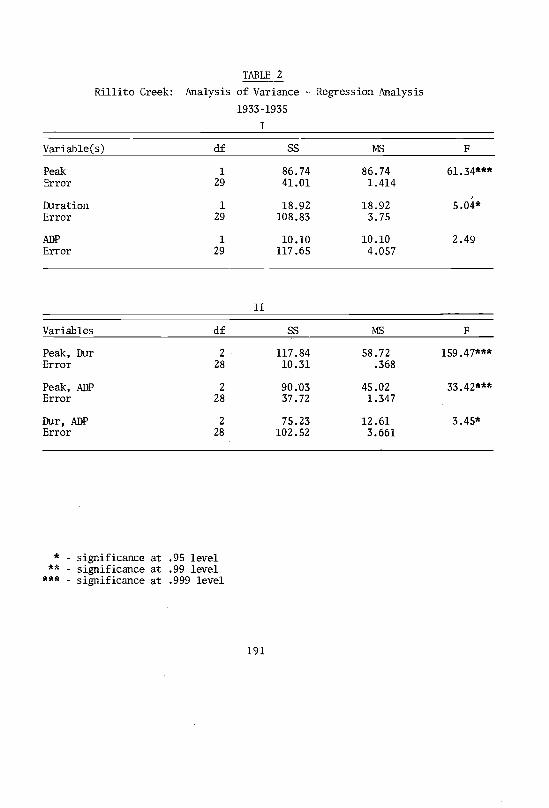
TABLE 2


1933 -1935

I


Peak 1 86.74 86.74 61.34 * **

Error 29 41.01 1.414

Duration 1 18.92 18.92 5.04*Error 29 108.83 3.75

ADP 1 10.10 10.10 2.49Error 29 117.65 4.057

II


Peak, Dur 2 117.84 58.72 159.47 * **

Error 28 10.31 .368

Peak, ADP 2 90.03 45.02 33.42 * **

Error 28 37.72 1.347

Dur, ADP 2 75.23 12.61 3.45*Error 28 102.52 3.661



191

1933 -1935 -- continued

III


Peak, Dur, ADP 3 118.11 39.37 114.39 * **


Difference due to ADP 1 .68 .68 1.96

Peak, ADP 2 90.03 78.66 * **

Difference due to Dur 1 28.08 28.08

Dur, ADP 2 25.23 260.17 * **

Difference due to Peak 1 92.88 92.88

IV


Peak, Dur, ADP 3 118.11 39.37 114.39 * **

Error -Total 27 9.64 .357

Peak 1 86.74 43.93 * **

Difference due toDur, ADP 2 31.37 15.68

Dur 1 18.92 139.92 * **

Difference due toPeak, ADP 2 99.19 45.60

ADP 1 10.0 151.27 * **

Difference due toPeak, Dur 2 108.01 54.01


192

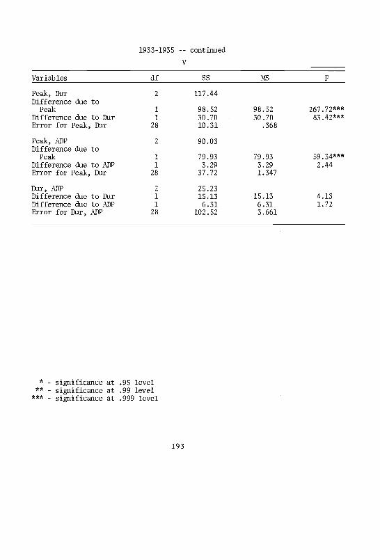
1933 -1935 -- continued

V


Peak, Dur 2 117.44Difference due to

Peak 1 98.52 98.52 267.72 * **



Peak, ADP 2 90.03Difference due to

Peak 1 79.93 79.93 59.34 * **

Difference due to ADP 1 3.29 3.29 2.44Error for Peak, Dur 28 37.72 1.347

Dur, ADP 2 25.23Difference due to Dur 1 15.13 15.13 4.13

Difference due to ADP 1 6.31 6.31 1.72Error for Dur, ADP 28 102.52 3.661


193

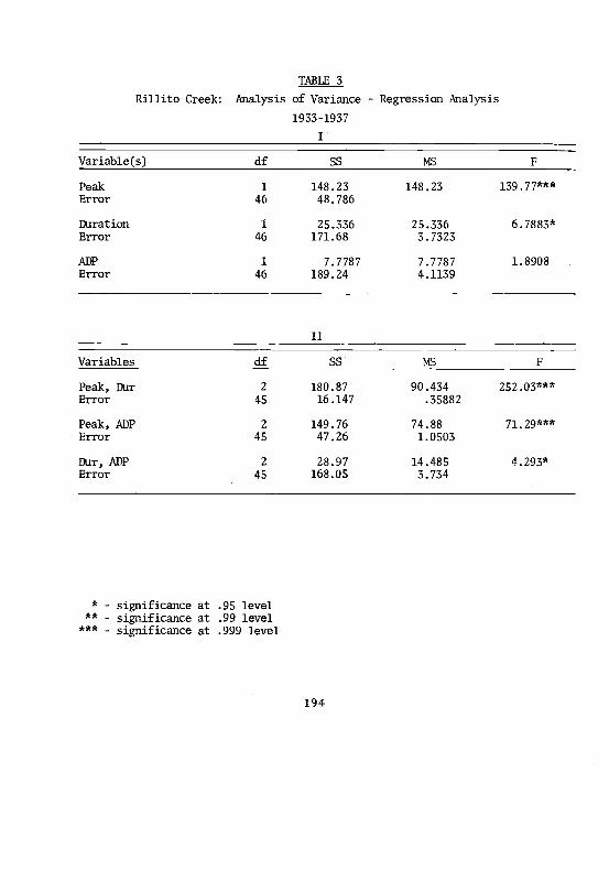
TABLE 3


1933 -1937

I


Peak 1 148.23 148.23 139.77 * **

Error 46 48.786

Duration 1 25.336 25.336 6.7883*Error 46 171.68 3.7323

ADP 1 7.7787 7.7787 1.8908Error 46 189.24 4.1139

II


Peak, Dur 2 180.87 90.434 252.03 * **

Error 45 16.147 .35882

Peak, ADP 2 149.76 74.88 71.29 * **

Error 45 47.26 1.0503

Dur, ADP 2 28.97 14.485 4.293*Error 45 168.05 3.734


194

1933 -1935 -- continued

III


Peak, Dur, ADP 3 180.89 60.297 164.55 * **

Error -Total 44 16.123 .36643

Peak, Dur 2 180.87Difference due to ADP 1 .024 .024 .0655

Peak, ADP 2 149.76Difference due to Dur 1 31.14 31.14 84.98 * **

Dur, ADP 2 28.97Difference due to

Peak 1 151.92 151.92 414.59 * **

IV


Peak, Dur, ADP 3 180.89 60.297 164.55 * **

Error -Total 44 16.123 .36643

Peak 1 148.23Difference due to Dur,ADP 2 32.66 16.33 44.56 * **

Dur 1 25.34Difference due to

Peak, ADP 2 155.55 77.78 212.25 * **

ADP 1 7.78Difference due to

Peak, Dur 2 173.11 86.55 236.21 * **


195

TABLE 4

Rillito Creek: Analysis of Variance - Regression

1933 -1942

Analysis


Peak 1 376.43 376.43 386.88 * **

Error 92 89.54 .973

Duration 1 103.85 103.85 26.39 * **

Error 92 362.12 3.93

ADP 1 21.84 21.84 4.52*Error 92 444.13 4.83

II


Peak, Dur 2 419.91 414.81 * **

Error 91 46.06 .506

Peak, ADP 2 376.91 192.56 * **Error 91 89.06 .979

Dur, ADP 2 117.36 15.32 * **Error 91 348.61 3.831


196

1933-1942 -- continued

III


Peak, Dur, ADP 3 417.98 139.32 261.29***


Peak, Dur 2 419.91

Difference due to ADP 1 .07 .07 .131


Dur, ADP 2 117.36Difference due to Peak 1 300.62 300.62 564.02 * **

IV


Peak, Dur, ADP 3 417.98 139.32 261.29 * **


Peak 1 376.43Difference due to Dur,

ADP 2 41.55 20.78 38.98 * **

Dur 1 103.85

Difference due toPeak, ADP 2 314.13 157.07 294.68 * **

ADP 1 21.84

Difference due toPeak, Dur 2 396.14 198.07 371.61 * **



197

1933-1942 -- continued

V


Peak, Dur 2 419.91

Difference due to Peak 1 316.06 316.06 624.62 * **


Error for Peak, Dur 91 46.06

Peak, ADP 2 376.91Difference due to Peak 1 355.07 355.07 362.69 * **


Error for Peak, ADP 91 89.06 .979

Dur, ADP 2 117.36Difference due to Dur 1 95.52 95.52 24.93

Difference due to ADP 1 13.51 13.51 3.53



198

TABLE 5


1933 -1951

I


Peak 1 818.00 818.00 1058.21 * **

Error 197 152.24 .773

Duration 1 241.01 241.01 65.11 * **

Error 197 729.23 3.702

ADP 1 9.05Error 197 961.19 4.879 1.86

II


Peak, Dur 2 888.56 444.28 1066.20 * **

Error 196 81.68 .4167

Peak, ADP 2 818.09 409.05 526.93 * **

Error 196 152.15 .7763

Dur, ADP 2 245.01 122.51 33.11 * **

Error 196 725.23 3.700



199

1933 -1951 -- continued

III


Peak, Dur, ADP 3 888.57 296.19 707.20 * **

Total error 195 81.67 .4188

Peak, Dur 2 888.56Difference due to ADP 1 .01 .01 .0239

Peak, ADP 2 818.09Difference due to Dur 1 70.48 70.48 168.29***

Dur, ADP 2 245.01Difference due to Peak 1 643.56 643.56 1536.68***

IV


Peak, Dur, ADP 3 888.56 296.19 707.20 * **

Total error 195 81.67 .4188

Peak 1 818.00Difference due to Dur,ADP 2 70.57 35.29 84.25 * **

Dur 1 241.01Difference due to Peak,ADP 2 647.56 323.78 773.11 * **

ADP 1 9.05Difference due to Peak,Dur 2 879.52 439.76 1050.05 * **


200

1933 -1951 -- continued

V


Peak, Dur 2 888.56Difference due to Peak 1 647.55 647.55 1554.00 * **






Dur, ADP 2 245.01Difference due to Dur 1 235.96 235.96 63.77 * **





201

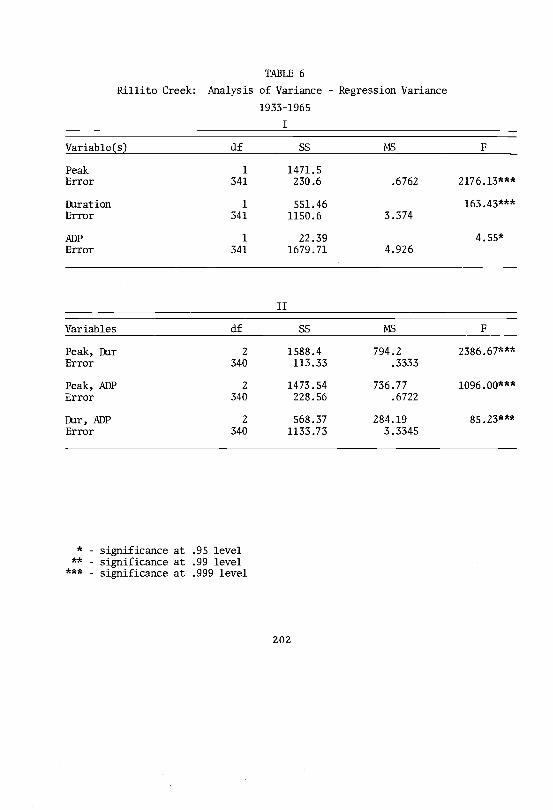
TABLE 6

Rillito Creek: Analysis of Variance - Regression Variance

1933 -1965

I


Peak 1 1471.5Error 341 230.6 .6762 2176.13 * **

Duration 1 551.46 163.43 * **

Error 341 1150.6 3.374

ADP 1 22.39 4.55*Error 341 1679.71 4.926

II


Peak, Dur 2 1588.4 794.2 2386.67 * **

Error 340 113.33 .3333

Peak, ADP 2 1473.54 736.77 1096.00 * **

Error 340 228.56 .6722

Dur, ADP 2 568.37 284.19 85.23 * **

Error 340 1133.73 3.3345


202

1933 -1951 -- continued

III


Peak, Dur, ADP 3 1588.8 529.6 1584.73 * **

Total error 339 113.29 .33419

Peak, Dur 2 1588.8Difference due to ADP 1 .4 .4 1.20


Dur, ADP 2 568.37Difference due to Peak 1 1020.43 1020.43 3053.44 * **

IV


Peak, Dur, ADP 3 1588.8 529.6 1584.73 * **

Total error 339 113.29 .33419

Peak 1 1471.5

Difference due to Dur,ADP 2 117.3 58.65 175.50 * **

Dur 1 551.46

Difference due to Peak,ADP 2 1037.34 518.67 1552.02 * **

ADP 1 22.39Difference due to Peak,

Dur 2 1566.41 783.21 2343.59



203

1933 -1951 -- continued

V


Peak, Dur 2 -1588.4

Difference due Peak 1 1036.94 3111.13 * **






Dur, ADP 2 568.37



Error for Dur, ADP 340 1133.73 3.3345


204

TABLE 7

Kolmogorov- Smirnov Test

Test to Test Differences Between Successive 2 -week Periods

a = .05 Critical level = .321 n = 36

Time Period Max o Result

Dec 15 -31 Jan 1 -15 .028 AcceptJan 1 -15 Jan 16 -31 .056 AcceptJan 16 -31 Feb 1 -15 .111 AcceptFeb 1 -15 Feb 15 -28 .139 AcceptFeb 15 -28 Mar 1 -15 .056 AcceptMar 1 -15 Mar 16 -31 .139 AcceptMar 16 -31 Apr 1 -15 .083 AcceptApr 16 -30 May 1 -15 .056 AcceptMay 1 -15 May 16 -31 0 AcceptMay 16 -31 June 1 -15 .028 AcceptJune 1 -15 June 16 -30 .056 AcceptJune 16 -30 July 1 -15 .250 AcceptJuly 1 -15 July 16 -31 .528 Reject * **

July 16 -31 Aug 1 -15 .139 AcceptAug 1 -15 Aug 16 -31 .167 AcceptAug 16 -31 Sept 1 -15 .444 Reject * **

Sept 1 -15 Sept 16 -31 .111 AcceptSept 16 -31 Oct 1 -15 .194 AcceptOct 1 -15 Oct 16 -31 .111 AcceptOct 16 -31 Nov 1 -15 .083 AcceptNov 1 -15 Nov 16 -31 .250 AcceptNov 16 -31 Dec 1 -15 .167 AcceptDec 1 -15 Dec 16 -31 .167 Accept

205

INSTANTANEOUSFLOW

(a) "ACTUAL" HYDROGRAPH

PEAK P

TOTAL FLOW F

DURATION D -I t =TIME

Figure 1(a). Hydrograph shape as a curvilinear triangle.

INSTANTANEOUS (b) COMPARISON OF ACTUAL ANDFLOW IDEALIZED HYDROGRAPH

EXACT COPY OF ABOVEHYDROGRAPH

IDEALIZEDHYDROGRAPHF= ODbi Pb2

D

Figure 1(b). Comparison of hydrographs as "pure" and curvilinear triangles.

206

UWo>Oz

I I I I I I

O Ií? O tn O tnM N N - - O

SM013 30 2:138Wf1N 39b'83n`d207

z

N O co

10-

8-w U Z w

6-U cr

4-

w m 2 Z

2-

RIL

LIT

O19

30T

HR

UCR

EE

K19

65

r__-

r0

I2

34

56

78

NU

MB

ER

OF

FLO

WS

BE

TW

EE

N A

UG

.I T

HR

U A

UG

.15

Figure 3.

Distribution of 0, 1, 2,

... flow arrivals between Aug. 1 and

Aug. 15 for the period 1930 -1965 on Rillito Creek.

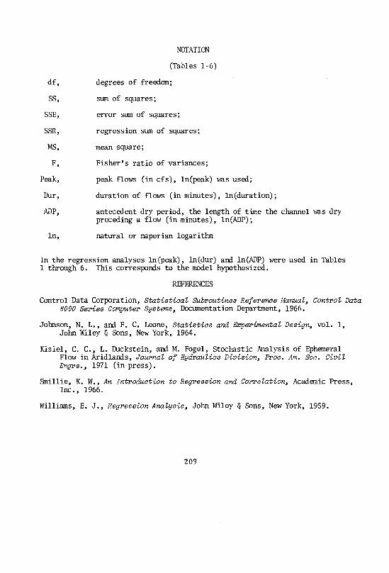
NOTATION

(Tables 1 -6)

df, degrees of freedom;

SS, sum of squares;

SSE, error sum of squares;

SSR, regression sum of squares;

MS, mean square;

F, Fisher's ratio of variances;

Peak, peak flows (in cfs), ln(peak) was used;

Dur, duration of flows (in minutes), ln(duration);

ADP, antecedent dry period, the length of time the channel was drypreceding a flow (in minutes), ln(ADP);

ln, natural or naperian logarithm

In the regression analyses ln(peak), ln(dur) and ln(ADP) were used in Tables1 through 6. This corresponds to the model hypothesized.

REFERENCES

Control Data Corporation, Statistical Subroutines Reference Manual, Control Data6000 Series Computer Systems, Documentation Department, 1966.

Johnson, N. L., and F. C. Leone, Statistics and Experimental Design, vol. 1,John Wiley $ Sons, New York, 1964.

Kisiel, C. C., L. Duckstein, and M. Fogel, Stochastic Analysis of EphemeralFlow in Aridlands, Journal of Hydraulics Division, Proc. Am. Soc. CivilEngrs., 1971 (in press).

Smillie, K. W., An Introduction to Regression and Correlation, Academic Press,Inc., 1966.

Williams, E. J., Regression Analysis, John Wiley & Sons, New York, 1959.

209

Acknowledgements. The work upon which this paper is based wassupported in part by funds provided by the United States Department ofthe Interior, Office of Water Resources Research, as authorized under theWater Resources Research Act of 1964. The computations were done at theUniversity of Arizona Computer Center on the CDC -6400 installed there.

210

N. E. BARAN C. C. KISIEL L. DUCKSTEIN...

Documents

Transcript of N. E. BARAN C. C. KISIEL L. DUCKSTEIN...