JHEP01(2017)019

Published for SISSA by Springer

Received: August 5, 2016

Accepted: December 24, 2016

Published: January 5, 2017

Duality walls and defects in 5d N = 1 theories

Davide Gaiotto and Hee-Cheol Kim

Perimeter Institute for Theoretical Physics,

31 Caroline Street North, Waterloo, ON N2L 2Y5 Canada

E-mail: dgaiotto@gmail.com, heecheol1@gmail.com

Abstract: We propose an explicit description of “duality walls” which encode at low

energy the global symmetry enhancement expected in the UV completion of certain five-

dimensional gauge theories. The proposal is supported by explicit localization computa-

tions and implies that the instanton partition function of these theories satisfies novel and

unexpected integral equations.

Keywords: Duality in Gauge Field Theories, Field Theories in Higher Dimensions, Su-

persymmetric gauge theory, Supersymmetry and Duality

ArXiv ePrint: 1506.03871

Open Access, c© The Authors.

Article funded by SCOAP3.doi:10.1007/JHEP01(2017)019

JHEP01(2017)019

Contents

1 Introduction 2

2 Duality walls between SU(N) gauge theories 3

2.1 Pure N = 1 SU(N)N gauge theory 3

2.1.1 Domain wall actions 5

2.2 SU(N)N−Nf/2 SQCD with Nf < 2N flavors 8

2.3 Duality walls for SU(N) with Nf = 2N 11

2.4 Linear quivers 12

2.5 Exceptional symmetries in SU(2) theories 14

3 Index calculations 16

3.1 SU(N)N theories 16

3.1.1 Example: SU(N)N−Nf/2 theories with Nf flavors 20

4 Wilson loops 21

4.1 Hemispheres with Wilson loop insertions 22

4.2 Example: SU(2) theories 24

4.3 Example: SU(3) theories 24

5 Duality and ’t Hooft surfaces 25

5.1 Higgsing IN,N 25

6 Codimension 2 defects 29

6.1 Higgsing in the absence of a duality wall 29

6.2 Higgsing in the presence of a duality wall 31

7 Duality walls between Sp(N) and SU(N + 1) theories 32

7.1 Enhanced symmetry of SU(N + 1) theory 34

7.2 From Sp(N) to exotic SU(N + 1) 37

7.3 Wilson loops 40

A 5d Nekrasov’s instanton partition function 42

A.1 SU(N) partition function 44

A.2 Sp(N) partition function 45

A.3 Hypermultiplets 46

B Partition functions of exotic SU(3) theory 48

B.1 Superconformal indices 52

– 1 –

JHEP01(2017)019

1 Introduction

Five-dimensional super-conformal field theories are a particularly rich subject of investi-

gation (see [1–5] for seminal work on the subject). The only constructions available for

these theories involve brane constructions, in particular quarter-BPS webs of five-branes

in IIB string theory. Some of the five-dimensional SCFTs admit mass deformations to

five-dimensional gauge theories, with the inverse gauge coupling playing the role of mass

deformation parameter. Several protected quantities in the five-dimensional SCFT are

computable directly from the low-energy gauge-theory description [6].

More precisely, the space of mass deformations of the UV SCFT is usually decomposed

into chambers, which flow in the IR to distinct-looking gauge theories, or to the same gauge

theory but with different identifications of the parameters. With some abuse of language,

these distinct IR theories may be thought of as being related by an “UV duality”, in the

sense that protected calculations in these IR theories should match [7].

In such a situation, one may define the notion of “duality walls” between the different

IR theories [8]. These are half-BPS interfaces which we expect to arise from RG flows

starting from Janus-like configurations, where the mass deformation parameters vary con-

tinuously in the UV, interpolating between two chambers. Duality walls between different

chambers should compose appropriately.

Furthermore, if we have some BPS defect in the UV SCFT, we have in principle

a distinct IR image of the defect in each chamber, each giving the same answer when

inserted in protected quantities. The duality walls should intertwine, in an appropriate

sense, between these images.

In this paper we propose candidate duality walls for a large class of quiver gauge

theories of unitary groups.1 The UV completion of these gauge theories has a conjectural

enhanced global symmetry whose Cartan generators are the instanton number symmetries

of the low-energy gauge theory. The chambers in the space of real mass deformations

dual to these global symmetries are Weyl chambers and the duality walls generate Weyl

reflections relating different chambers.

The duality walls admit a Lagrangian description in the low energy gauge theory. The

fusion of interfaces reproduces the expected relations for the Weyl group generators thanks

to a beautiful collection of Seiberg dualities. This is the first non-trivial check of our

proposal. The second set of checks involve the computation of protected quantities.

The duality walls we propose give a direct physical interpretation to a somewhat

unfamiliar object: elliptic Fourier transforms (see [10] and references within). These are

invertible integral transformations whose kernel is built out of elliptic gamma functions. We

interpret the integral kernel as the superconformal index of the four-dimensional degrees

of freedom sitting at the duality interface and the integral transform as the action of the

duality interface on more general boundary conditions for the five-dimensional gauge theory.

The integral identity which encodes the invertibility of the elliptic Fourier transform follows

from the corresponding Seiberg duality relations.

1Duality walls of the same kind, for 5d gauge theories endowed with a six-dimensional UV completion,

appeared first in [9].

– 2 –

JHEP01(2017)019

It follows directly from the localization formulae on the S4 × S1 and the definition

of a duality wall that the corresponding elliptic Fourier transform acting on the instanton

partition function of the gauge theory should give back the same partition function, up to

the Weyl reflection of the instanton fugacity. This is a surprising, counterintuitive integral

relation which should be satisfied by the instanton partition function. Amazingly, we find

that this relation is indeed satisfied to any order in the instanton expansion we cared to

check. This is a very strong test of our proposal.

Experimentally, we find that this is the first example of an infinite series of integral

identities, which control the duality symmetries of Wilson line operators. These relations

suggest how to assemble naive gauge theory Wilson line operators into objects which can

be expected to have an ancestor in the UV SCFT which is invariant under the full global

symmetry group.

We also identify a few boundary conditions and interfaces in the gauge theory which

transform covariantly under the action of the duality interface and could thus be good

candidates for symmetric defects in the UV SCFT. We briefly look at duality properties of

defects in codimension two and three as well.

Finally, we attempt to give a physical explanation to another instance of elliptic Fourier

transform which we found in the literature, which schematically appears to represent an

interface between an Sp(N) and an SU(N +1) gauge theories. We find that the AC elliptic

Fourier transform maps the instanton partition function of an Sp(N) gauge theory into the

instanton partition function of an exotic version of SU(N + 1) gauge theory with the same

number of flavors.

After this work was completed, we received [11, 12] which have some overlap with the

last section of this paper.

2 Duality walls between SU(N) gauge theories

2.1 Pure N = 1 SU(N)N gauge theory

Our first and key example of duality wall encodes the UV symmetries of a pure five-

dimensional N = 1 SU(N) gauge theory, with 5d CS coupling N .

This gauge theory is expected to be a low-energy description of a 5d SCFT with SU(2)

global symmetry, deformed by a real mass associated to the Cartan generator of SU(2).

In turn, the SCFT can be engineered by a BPS five-brane web involving four semi-infinite

external legs: two parallel NS5 branes, a (−1, N) and a (−1,−N) fivebranes. The SU(2)

global symmetry is associated to the two parallel NS5 branes. See figure 1.

The mass deformation breaks SU(2) to a U(1) subgroup, which is identified with the

instanton U(1)in global symmetry of the SU(N) gauge theory, whose current is the instanton

number density Jin = 18π2 TrF ∧F . The (absolute value of) the real mass is identified with

m = g−2YM in the IR and with the separation between the parallel NS5 branes in the UV.

The Weyl symmetry acts as m→ −m and the corresponding duality wall should relate

two copies of the same gauge theory, glued at the interface in such to preserve the anti-

diagonal combination of the U(1)in instanton global symmetries on the two sides of the

interface.

– 3 –

JHEP01(2017)019

m

(1,0)

(-1,-N) (-1,N)

(1,0)

N x (0,1)

Figure 1. The fivebrane web which engineers the UV completion of pure SU(N)N gauge theory.

The gauge theory is supported on the bundle of N parallel D5 branes. After removing the centre

of mass, the only non-normalizable deformation is the separation m between the NS5 branes.

SU(N) SU(N)

Figure 2. Our schematic depiction of the duality wall. We denote 5d gauge groups on the two

sides of an interface as open circles and the bi-fundamental matter as an arrow between them. The

extra baryonic coupling is denoted as a black dot over the arrow.

We propose the following setup: a domain wall defined by Neumann b.c. for the

SU(N)N gauge theory on the two sides of the wall, together with a set of bi-fundamental

4d chiral multiplets q living at the wall, coupled to an extra chiral multiplet b by a 4d

superpotential

W = b det q . (2.1)

See figure 2 for a schematic depiction of the duality wall.

This system is rife with potential gauge, mixed and global anomalies at the interface,

which originate from the 4d degrees of freedom, from the boundary conditions of the 5d

gauge fields and and from anomaly inflow from the bulk Chern-Simons couplings.

The cubic gauge anomaly cancels out beautifully: the bi-fundamental chiral multiplets

behave as N fundamental chiral multiplets for the gauge group on the right of the wall,

giving N units of cubic anomaly, which cancel against the anomaly inflow from the N units

of five-dimensional Chern-Simons coupling. Similarly, we get −N units of cubic anomaly

for the gauge group on the left of the wall, which also cancel against the anomaly inflow

from the N units of five-dimensional Chern-Simons coupling.

The bi-fundamental chiral multiplets also contribute to a mixed anomaly between the

bulk gauge fields and the baryonic U(1)B symmetry which rotates the bi-fundamental fields

with charge 1/N (normalized so that the baryon B = det q has charge 1). The anomaly

involving the left gauge fields has the same sign and magnitude as the anomaly involving

– 4 –

JHEP01(2017)019

SU(N) SU(N) SU(N)

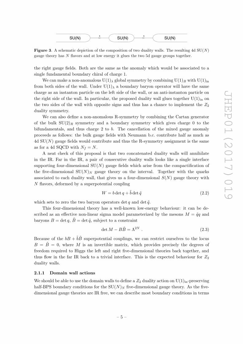
Figure 3. A schematic depiction of the composition of two duality walls. The resulting 4d SU(N)

gauge theory has N flavors and at low energy it glues the two 5d gauge groups together.

the right gauge fields. Both are the same as the anomaly which would be associated to a

single fundamental boundary chiral of charge 1.

We can make a non-anomalous U(1)λ global symmetry by combining U(1)B with U(1)in

from both sides of the wall. Under U(1)λ a boundary baryon operator will have the same

charge as an instanton particle on the left side of the wall, or an anti-instanton particle on

the right side of the wall. In particular, the proposed duality wall glues together U(1)in on

the two sides of the wall with opposite signs and thus has a chance to implement the Z2

duality symmetry.

We can also define a non-anomalous R-symmetry by combining the Cartan generator

of the bulk SU(2)R symmetry and a boundary symmetry which gives charge 0 to the

bifundamentals, and thus charge 2 to b. The cancellation of the mixed gauge anomaly

proceeds as follows: the bulk gauge fields with Neumann b.c. contribute half as much as

4d SU(N) gauge fields would contribute and thus the R-symmetry assignment is the same

as for a 4d SQCD with Nf = N .

A neat check of this proposal is that two concatenated duality walls will annihilate

in the IR. Far in the IR, a pair of consecutive duality walls looks like a single interface

supporting four-dimensional SU(N) gauge fields which arise from the compactification of

the five-dimensional SU(N)N gauge theory on the interval. Together with the quarks

associated to each duality wall, that gives us a four-dimensional S(N) gauge theory with

N flavors, deformed by a superpotential coupling

W = b det q + b det q (2.2)

which sets to zero the two baryon operators det q and det q.

This four-dimensional theory has a well-known low-energy behaviour: it can be de-

scribed as an effective non-linear sigma model parameterized by the mesons M = qq and

baryons B = det q, B = det q, subject to a constraint

detM −BB = Λ2N . (2.3)

Because of the bB + bB superpotential couplings, we can restrict ourselves to the locus

B = B = 0, where M is an invertible matrix, which provides precisely the degrees of

freedom required to Higgs the left and right five-dimensional theories back together, and

thus flow in the far IR back to a trivial interface. This is the expected behaviour for Z2

duality walls.

2.1.1 Domain wall actions

We should be able to use the domain walls to define a Z2 duality action on U(1)in-preserving

half-BPS boundary conditions for the SU(N)N five-dimensional gauge theory. As the five-

dimensional gauge theories are IR free, we can describe most boundary conditions in terms

– 5 –

JHEP01(2017)019

of their boundary degrees of freedom, which are in general some four-dimensional SCFTs

equipped with an SU(N) and an U(1)in global symmetries with specific cubic anomalies.

The exceptions are boundary conditions which (partially) break the gauge symmetry at

the boundary.

More precisely, consider a 4d N = 1 theory B with a SU(N) global symmetry with N

units of cubic ’t Hooft anomaly, a U(1)∂ global symmetry with a mixed ’t Hooft anomaly

with the SU(N) global symmetry equal to the contribution of a single fundamental chiral

field of charge 1 and an R-symmetry with a mixed ’t Hooft anomaly with the SU(N) global

symmetry equal to the contribution of N quarks of R-charge 0. Such a theory can be used

to define a boundary condition for the 5d SU(N)N gauge theory which preserves a U(1)λsymmetry, diagonal combination of U(1)in and U(1)∂ , and an R-symmetry.

The action of the duality wall on this boundary condition gives a new theory B′ built

from B by adding N anti-fundamental chiral multiplets q of SU(N), gauging the overall

SU(N) global symmetry and adding the W = b det q superpotential. The new theory has

the same type of mixed ’t Hooft anomalies as we required for B (involving a new choice of

U(1)∂ global symmetry).

In case of boundary conditions which break the gauge group to some subgroup H, we

can apply a similar transformation, which only gauges the H subgroup of SU(N). For

example, the duality wall maps Dirichlet boundary conditions, which fully break the gauge

group at the boundary, to Neumann boundary conditions enriched by the set of N chiral

quarks q and the b chiral field with W = b det q, and vice-versa.2

We can provide a more entertaining example: a self-dual boundary condition. We

define the boundary condition by coupling the five-dimensional gauge fields to N+1 quarks

q′ and a single anti-quark q′. For future convenience, we also add N + 1 extra chiral

multiplets M coupled by the superpotential

q′q′M . (2.4)

Thus the boundary condition has an extra SU(N + 1) × U(1)e global symmetries defined

at the boundary. The SU(N + 1) simply rotates q′ as anti-fundamentals and M as funda-

mentals. The non-anomalous R-symmetry assignments are akin to the ones for a 4d SQCD

with N + 1 flavors.

The bulk instanton symmetry can be extended to a non-anomalous symmetry under

which the quarks have charge 1/N and anti-quarks have charge −1/N . The remaining non-

anomalous boundary U(1)e will act on quarks with charge 1/N , anti-quarks with charge

−1− 1/N and on M with charge 1.

After acting with the duality interface, we find at the boundary four-dimensional

SU(N) gauge theory, with N + 1 flavors given by the quarks q′ and anti-quarks q and

q′. The theory has a Seiberg dual description in the IR, involving the mesons and baryons

coupled by a cubic superpotential. The W = b det q + q′q′M lift the q′q′ mesons and the

2It may be possible to consider a larger set of boundary conditions, involving singular boundary condi-

tions for the matter and gauge fields, akin to Nahm pole boundary conditions for maximally supersymmetric

gauge theories [13, 14].

– 6 –

JHEP01(2017)019

SU(N) SU(M)

N+M

Figure 4. A schematic depiction of the duality-covariant interface IN,M . We include a superpo-

tential coupling for the closed loop of three arrows.

SU(N) SU(N) SU(M) SU(M)SU(M)

N+M

SU(M)

N+M

SU(N)

N+M

Figure 5. The Seiberg duality transformation which implies the duality-covariance of IN,M .

det q anti-baryon. The remaining qq′ mesons give N + 1 new fundamental chiral at the

boundary, the dual version of q′. The remaining anti-baryons give one anti-fundamental

chiral, the dual version of q′. The baryons give the dual version of M .

We should keep track of the Abelian global symmetries. The dual quarks have instan-

ton charge zero and U(1)e charge 1/N . The dual anti-quarks have instanton charge −1

and U(1)e charge −1− 1/N . The dual M has instanton charge 1 and U(1)e charge 1.

In order for the self-duality to be apparent, we should re-define our instanton symmetry

to act on the quarks q′ with charge 1/(2N), anti-quarks with charge 1/2− 1/(2N), on M

with charge −1/2. Then the action of the duality interface switches the sign of the instanton

charges, but leave U(1)e unaffected. It is natural to conjecture that this boundary condition

descends from an SU(2)in-invariant boundary condition for the UV SCFT, equipped with

an extra SU(N + 1)×U(1)e global symmetry.

We can generalize that to a duality-covariant interface IN,N ′ between SU(N)N and

SU(N ′)N ′ , coupled to three sets of four-dimensional chiral fields: N +N ′ fundamentals w

of SU(N), N+N ′ anti-fundamentals u of SU(N ′) and a set of bi-fundamentals v of SU(N ′)

and SU(N), coupled by a cubic superpotential W = uvw.

If we act with an SU(N)N duality interface, we obtain a four-dimensional SU(N)

gauge theory with N + N ′ flavors, fundamentals w and anti-fundamentals v and q. Ap-

plying Seiberg duality, we arrive to an SU(N ′) gauge theory with N + N ′ flavors. The

original superpotential lifts the u fields and the vw mesons. The b det q superpotential

maps to a similar b det q∨ involving the Seiberg-dual quarks which transform under the

five-dimensional SU(N ′)N ′ gauge fields. The final result is identical as what one would

obtain by acting with the SU(N ′)N ′ duality interface.

The duality-covariant interfaces IN,N ′ have interesting properties under composition.

Consider the composition of IN,N ′ and IN ′,N ′′ : it supports a four-dimensional SU(N ′) gauge

theory coupled to N + N ′ + N ′′ flavors, which include the N + N ′ anti-fundamentals u,

N ′ +N ′′ fundamentals w′, bifundamentals v and v′. If we apply Seiberg duality, we find a

new description of a composite interface, which is actually a modification of IN,N ′′ ! Indeed,

we find an SU(N +N ′′) gauge group which is coupled to the 5d degrees of freedom just as

the flavor group of IN,N ′′ , and is furthermore coupled to N+N ′ fundamentals and N ′+N ′′

– 7 –

JHEP01(2017)019

m

(1,0)

(-1,-N)

(-1,Nf - N)

(-1,N)

(1,0)

N x (0,1)

Nf x (0,1)

mf

mf’

m

(1,0)

(1,Nf)

(-1,Nf - N)

(-1,N)

(1,0)

N x (0,1)

Nf x (0,1)

-mf

mf’

Figure 6. The fivebrane web which engineers the UV completion of SU(N)N−Nf/2 SQCD. The

gauge theory is supported on the bundle of N parallel D5 branes. After removing the centre of mass,

the non-normalizable deformation are the separation m between the NS5 branes and the vertical

separation mf between the semi-infinite D5 branes and the intersection of one of the NS5 branes and

the (−1, N) fivebrane. The latter parameter is the overall mass parameter for the hypermultiplets.

We drew the resolved fivebrane web for positive and negative values of the overall hypermultiplet

mass. The former is closely related, but not identical to the gauge coupling or mass for U(1)in. It

is possible to argue that the instanton mass mi actually equals m+Nf

2 mf . The standard IR gauge

theory description is valid for m > 0 and m+Nfmf > 0. When m becomes negative and we flip its

sign to go to a dual parameterization, we exchange the roles of the NS5 branes and thus the role of

mf and the auxiliary parameter m′f = mf + mN . Alternatively, we can use

mf+m′f2 as a parameter,

which remains invariant under duality.

anti-fundamentals with a superpotential coupling to (N +N ′)× (N ′ +N ′′) mesons. This

is consistent with the duality-covariance of the interface.

The interface IN,N ′ clearly has an SU(N + N ′) global symmetry. We can also define

an U(1)e non-anomalous global symmetry, acting with charge 1 on v, − N ′

N+N ′ on w and

− NN+N ′ on u. The second U(1)in global symmetry can be taken to act with charge 1 on w,

−1 on u and charge N +N ′ on instantons on the two sides.

The IN,N duality-covariant interface is particularly interesting. It supports a baryon

operator det v charged under U(1)e only. If we give it a vev, by a diagonal vev of v, we

Higgs together the gauge fields on the two sides of the interface and the superpotential

coupling gives a mass to u and w. We arrive to a trivial interface. Later on in section 5

we will use IN,N to study the duality properties of of ’t Hooft surface defects.

2.2 SU(N)N−Nf/2 SQCD with Nf < 2N flavors

A similar UV promotion of U(1)in to SU(2) is expected to hold for SU(N)N−Nf/2 5d gauge

theories with Nf flavors, with Nf < 2N . The SCFT can be engineered by a BPS five-brane

web involving Nf + 4 semi-infinite external legs: two parallel NS5 branes, a (−1, N) and a

(−1, Nf −N) fivebranes, Nf D5 branes pointing to the left. The SU(2) global symmetry is

associated again to the two parallel NS5 branes, while the Nf D5 branes support an U(Nf )

global symmetry. The fivebrane webs and mass parameters are depicted in figure 6.

– 8 –

JHEP01(2017)019

As the gauge fields are IR free, we expect to be able to describe a typical half-

BPS boundary condition for such gauge theories in terms of an SU(N)-preserving bound-

ary conditions for the five-dimensional hypermultiplets, with a weak gauging of the five-

dimensional SU(N) symmetry. Of course, it is also possible to only preserve, and gauge, at

the boundary some smaller subgroup H of the five-dimensional gauge group. An extreme

example would be to give Dirichlet boundary conditions to the gauge fields.

Half-BPS boundary conditions for five-dimensional free hypermultiplets may yet be

strongly coupled. On general grounds [15], it is always possible, up to D-terms, to de-

scribe such boundary conditions as deformations of simple boundary conditions which set

a Lagrangian half of the hypermultiplet scalars (which we can denote as “Y”) to zero at

the boundary. The remaining hypers (which we can denote as “X”) can be coupled to a

boundary theory B by a linear superpotential coupling

W = XO (2.5)

involving some boundary operator O. This gives a boundary condition which we could

denote as BX .

Conversely, if we are given some boundary condition BX for free hypermultiplets, we

can produce a four-dimensional theory B by putting the 5d hypers on a segment, with

boundary conditions BX on one side and X = 0 on the other side. Up to D-terms, this

inverts the map B → BX , with O being the value of Y at the X = 0 boundary.

In particular, a boundary condition X = 0 can be engineered by a theory B consisting of

free chiral multiplets φ with the same quantum numbers as Y , and superpotential W = Xφ.

The trivial interface can be obtained from a Y = 0, X ′ = 0 boundary condition by a

W = XY ′ superpotential coupling, where the primed and un-primed fields live on the two

sides of the interface.

With these considerations in mind, we can evaluate the ’t Hooft anomaly polynomial

for a boundary condition Y = 0: because of the symmetry between X = 0 and Y = 0, it

must be exactly half of the ’t Hooft anomaly polynomial for a four-dimensional free chiral

with the same quantum numbers as X.

Our proposal for the duality interface generalizes the interface for pure SU(N)N gauge

theory: we set to zero at the boundary the fundamental half X of the hypermultiplets

on the right of the wall and anti-fundamental Y ′ on the left of the wall, with a boundary

superpotential

W = b det q + TrX ′qY . (2.6)

The combination of gauge anomalies from q and the boundary condition for the hyper-

multiplet precisely matches the desired bulk Chern-Simons level N −Nf/2. We denote as

X the fields which transform as anti-fundamentals of U(Nf ). In particular, we give them

charge −1 under the diagonal U(1)f global symmetry in U(Nf ).

A consecutive pair of these conjectural duality walls can be analyzed just as in the pure

gauge theory case, as the boundary conditions prevent the five-dimensional hypers on the

interval from contributing extra light four-dimensional fields. They can be integrated away

to give a TrX ′′qqY coupling. As the meson qq is identifies with the identity operator in the

– 9 –

JHEP01(2017)019

SU(N) SU(N)

Nf

Figure 7. Our schematic depiction of the duality wall for SQCD. We denote the 5d SU(Nf ) flavor

group which goes through the interface as a strip. The dashed arrows indicate which half of the

bulk hypermultiplets survives at the wall. We include a superpotential coupling for the closed loop

of three arrows.

Nf

SU(N) SU(N) SU(N)

Figure 8. A schematic depiction of the composition of two duality wall for SQCD. The resulting

4d SU(N) gauge theory has N flavors and at low energy it glues the two 5d gauge groups together.

The theory includes a quartic superpotential coupling which arises from integrating away the hy-

permultiplets in the segment. In the IR, it glues together the hypermultiplets on the two sides of

the interface.

IR, the interface flows to a trivial interface for both the gauge fields and the hypermultiplets,

up to D-terms. Thus the interface is a reasonable candidate for a duality wall.

Next, we can look carefully at the anomaly cancellation conditions. It is useful to

express the anomaly cancellation in terms of fugacities. If we ignore for a moment the

R-charge and say that q has fugacity λ1/N , X has fugacity x and X ′ has fugacity x′, the

superpotential imposes x = λ1/Nx′, anomaly cancellation for the left gauge group sets the

instanton fugacities on the right to ir = λx−Nf/2 and i` = λ−1(x′)−Nf/2.

We can re-cast the relation as a statement about one combination of bulk fugacity

being inverted by the interface, λ = irxNf/2 and λ−1 = i`(x

′)Nf/2, and one being not

inverted irxNf/2−2N = i`(x

′)Nf/2−2N .

Although these relations may look unfamiliar, they can be understood in a straight-

forward way in therms of the (p, q) fivebrane construction of SU(N)N−Nf/2. Indeed, λ is

the fugacity which is associated to the mass parameter m and x−1 to mf , (x′)−1 to m′f .

As far as R-symmetry is concerned, the bulk R-symmetry only acts on the scalar fields

in the hypermultiplets, with charge 1. Thus we expect that assigning R-symmetry 0 to q

and 2 to b will both satisfy anomaly cancellation and be compatible with the superpotential

couplings.

It is straightforward to extend to SQCD the duality-covariant boundary conditions

and interfaces proposed for pure SU(N) gauge theory. We refer to figure 9 for the quiver

description of the IN,M interface and to figure 10 for the Seiberg-duality proof of duality-

covariance. The composition of IN,M and IM,S can again be converted to a modification

of IN,S .

– 10 –

JHEP01(2017)019

Nf

SU(N) SU(M)

N+M-Nf

Figure 9. A schematic depiction of the duality-covariant interface IN,M . We include a superpo-

tential coupling for the closed loops of three arrows.

Nf Nf

N+M-NfN+M-Nf

SU(N) SU(N) SU(M) SU(M)SU(M)SU(M) SU(N)

Figure 10. The Seiberg duality transformation which implies the duality-covariance of IN,M .

m

m’

(1,0)

(1,2N)

(-1,N)

(1,0)

N x (0,1)

2N x (0,1)

(-1,N)

-mf

mf’

Figure 11. The fivebrane web which engineers the UV completion of SU(N)0, Nf = 2N SQCD.

After removing the centre of mass, the non-normalizable deformation are the separation m between

the NS5 branes and the separation m between the (−1, N) fivebranes. The vertical separation mf

between the semi-infinite D5 branes and the intersection of one of the NS5 branes and the (−1, N)

fivebrane and instanton mass mi are related to m and m′ as m = mi −Nmf , m′ = mi +Nmf .

2.3 Duality walls for SU(N) with Nf = 2N

The SU(N) theory with 2N flavors is rather special: in the UV, two distinct Abelian global

symmetries are expected to be promoted to an SU(2). Essentially, they are the sum and

difference of the instanton and baryonic U(1) isometries. Correspondingly, we will find two

commuting duality walls. In the fivebrane construction, the extra symmetry is due to two

sets of parallel fivebranes. See figure 11.

The first duality wall is defined precisely as before, i.e. set to zero at the boundary the

fundamental half X of the hypermultiplets on the right of the wall and anti-fundamental

– 11 –

JHEP01(2017)019

SU(N) SU(N)

2N

SU(N) SU(N)

2N

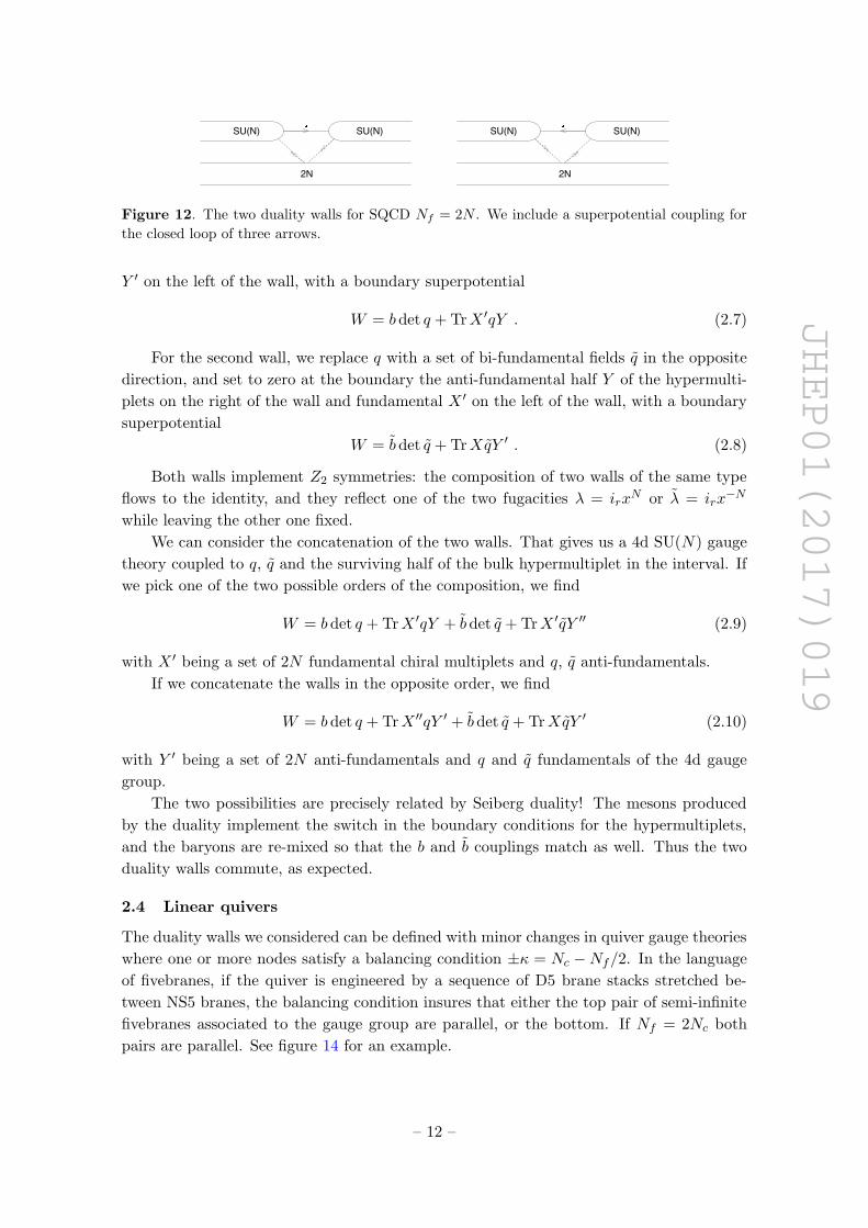
Figure 12. The two duality walls for SQCD Nf = 2N . We include a superpotential coupling for

the closed loop of three arrows.

Y ′ on the left of the wall, with a boundary superpotential

W = b det q + TrX ′qY . (2.7)

For the second wall, we replace q with a set of bi-fundamental fields q in the opposite

direction, and set to zero at the boundary the anti-fundamental half Y of the hypermulti-

plets on the right of the wall and fundamental X ′ on the left of the wall, with a boundary

superpotential

W = b det q + TrXqY ′ . (2.8)

Both walls implement Z2 symmetries: the composition of two walls of the same type

flows to the identity, and they reflect one of the two fugacities λ = irxN or λ = irx

−N

while leaving the other one fixed.

We can consider the concatenation of the two walls. That gives us a 4d SU(N) gauge

theory coupled to q, q and the surviving half of the bulk hypermultiplet in the interval. If

we pick one of the two possible orders of the composition, we find

W = b det q + TrX ′qY + b det q + TrX ′qY ′′ (2.9)

with X ′ being a set of 2N fundamental chiral multiplets and q, q anti-fundamentals.

If we concatenate the walls in the opposite order, we find

W = b det q + TrX ′′qY ′ + b det q + TrXqY ′ (2.10)

with Y ′ being a set of 2N anti-fundamentals and q and q fundamentals of the 4d gauge

group.

The two possibilities are precisely related by Seiberg duality! The mesons produced

by the duality implement the switch in the boundary conditions for the hypermultiplets,

and the baryons are re-mixed so that the b and b couplings match as well. Thus the two

duality walls commute, as expected.

2.4 Linear quivers

The duality walls we considered can be defined with minor changes in quiver gauge theories

where one or more nodes satisfy a balancing condition ±κ = Nc −Nf/2. In the language

of fivebranes, if the quiver is engineered by a sequence of D5 brane stacks stretched be-

tween NS5 branes, the balancing condition insures that either the top pair of semi-infinite

fivebranes associated to the gauge group are parallel, or the bottom. If Nf = 2Nc both

pairs are parallel. See figure 14 for an example.

– 12 –

JHEP01(2017)019

SU(N) SU(N)

2N

SU(N)

SU(N) SU(N)

2N

SU(N)

Figure 13. The Seiberg duality demonstrating how the two duality walls for SQCD Nf = 2N

commute.

m

m’

m’’

(1,0)

(1,0)

(1,0)

(-1,0)

(-1,0)

(1,N)

(1,N)

(1,N)

(-1,N-M)

N x (0,-1)

N x (0,1)

N x (0,1)

M x (0,1)

-mf

-mf’

-mf’’

Figure 14. The fivebrane web which engineers the UV completion of a SU(N) × SU(N) gauge

theory with N flavors at the left node and M at the right node. The five U(1) global symmetries

(two instanton symmetries and three hypermultiplet masses) are enhanced to U(1)2×SU(2)×SU(3)

because of the two sets of parallel fivebranes. The six mass deformations in the picture satisfy a

relation: m′ = m+Mmf +Nm′f .

A sequence of k balanced nodes is expected to be associated in the UV to an SU(k+1)

global symmetry, enhancing a certain combination of the instanton and bi-fundamental

hypermultiplet charges for these nodes.

We want to understand the effect of a duality wall for a node of the quiver on the

other nodes of the quiver, and figure out how the duality walls for different nodes match

together.

We can define the duality wall at a balanced node as we did for a single gauge group,

leaving the other gauge groups and other hypermultiplets continuous at the interface.

As the X ′ and Y fields for a given node are charged under the gauge groups at nearby

nodes, but have different Abelian charges, in order for the corresponding symmetries to

– 13 –

JHEP01(2017)019

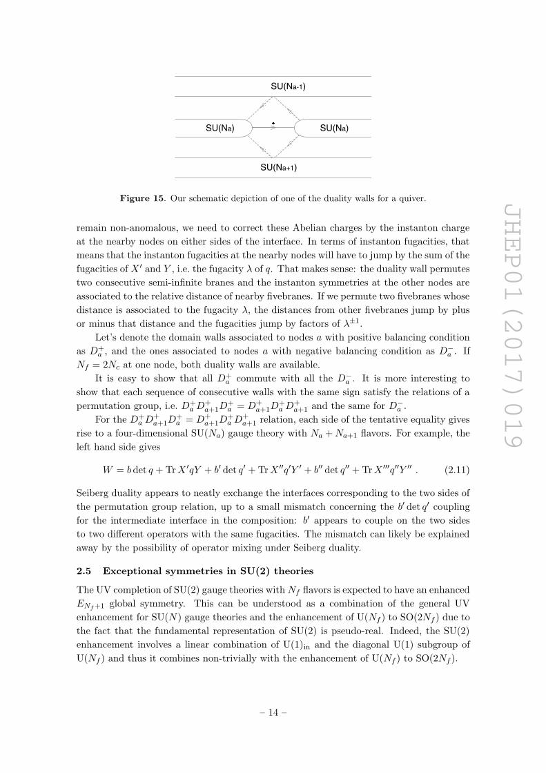
SU(Na) SU(Na)

SU(Na-1)

SU(Na+1)

Figure 15. Our schematic depiction of one of the duality walls for a quiver.

remain non-anomalous, we need to correct these Abelian charges by the instanton charge

at the nearby nodes on either sides of the interface. In terms of instanton fugacities, that

means that the instanton fugacities at the nearby nodes will have to jump by the sum of the

fugacities of X ′ and Y , i.e. the fugacity λ of q. That makes sense: the duality wall permutes

two consecutive semi-infinite branes and the instanton symmetries at the other nodes are

associated to the relative distance of nearby fivebranes. If we permute two fivebranes whose

distance is associated to the fugacity λ, the distances from other fivebranes jump by plus

or minus that distance and the fugacities jump by factors of λ±1.

Let’s denote the domain walls associated to nodes a with positive balancing condition

as D+a , and the ones associated to nodes a with negative balancing condition as D−a . If

Nf = 2Nc at one node, both duality walls are available.

It is easy to show that all D+a commute with all the D−a . It is more interesting to

show that each sequence of consecutive walls with the same sign satisfy the relations of a

permutation group, i.e. D+a D

+a+1D

+a = D+

a+1D+a D

+a+1 and the same for D−a .

For the D+a D

+a+1D

+a = D+

a+1D+a D

+a+1 relation, each side of the tentative equality gives

rise to a four-dimensional SU(Na) gauge theory with Na +Na+1 flavors. For example, the

left hand side gives

W = b det q + TrX ′qY + b′ det q′ + TrX ′′q′Y ′ + b′′ det q′′ + TrX ′′′q′′Y ′′ . (2.11)

Seiberg duality appears to neatly exchange the interfaces corresponding to the two sides of

the permutation group relation, up to a small mismatch concerning the b′ det q′ coupling

for the intermediate interface in the composition: b′ appears to couple on the two sides

to two different operators with the same fugacities. The mismatch can likely be explained

away by the possibility of operator mixing under Seiberg duality.

2.5 Exceptional symmetries in SU(2) theories

The UV completion of SU(2) gauge theories with Nf flavors is expected to have an enhanced

ENf+1 global symmetry. This can be understood as a combination of the general UV

enhancement for SU(N) gauge theories and the enhancement of U(Nf ) to SO(2Nf ) due to

the fact that the fundamental representation of SU(2) is pseudo-real. Indeed, the SU(2)

enhancement involves a linear combination of U(1)in and the diagonal U(1) subgroup of

U(Nf ) and thus it combines non-trivially with the enhancement of U(Nf ) to SO(2Nf ).

– 14 –

JHEP01(2017)019

Correspondingly, we can find continuously many versions of our basic duality wall,

each labelled by a choice of U(Nf ) subgroup in SO(2Nf ) and a splitting of the hypermul-

tiplet scalars into N “X” and N “Y” complex scalar fields. It is most useful to look at

domain walls which preserve a common Cartan sub-algebra of the global symmetry group,

implementing Weyl reflections in the UV.

If we denote the bulk quarks as Qi, i = 1, · · · , 2Nf , we can consider duality walls for

which the X fields consist of Nf − k quarks from the i = 1, · · · , Nf range and k quarks

from the i = Nf + 1, · · · , 2Nf range. If we denote as xa the fugacities of the quarks, the

overall fugacity of the X fields will be defined as xNf =∏a∈X xa. The domain walls invert

λ = ixNf/2 and leave ixNf/2−4 and the ratios xa/xa′ for a, a′ ∈ X fixed.

It is important to point out that not all splittings are simultaneously possible. There

are two disconnected classes of choices of X and Y fields among the Qi, distinguished

by comparing the sign of their “orientation” dX1dY1dX2dY2 · · · . Intuitively, in order to

interpolate between boundary conditions in different classes we need to add a single chiral

doublet at the boundary, which contributes one unit to the discrete Z2 gauge anomaly of

SU(2). Thus either boundary conditions with even k are simultaneously non-anomalous,

or boundary conditions with odd k are simultaneously non-anomalous, but not both.

Notice that SU(2) gauge theories have no continuous theta angle, but have a discrete

Z2-valued theta angle. One unit of discrete Z2 gauge anomaly at the boundary can be

compensated by a shift of the bulk discrete theta angle. Thus we expect the two classes

(even k and odd k) of boundary conditions to be associated to the two different choices of

bulk theta angle. Thus we have 2Nf−1 basic domain walls.

In general, composing two such domain walls associated to splittings (X,Y ) and

(X ′, Y ′) will give an interface supporting an 4d SU(2) gauge theory, with as many chi-

ral quarks as the number of bulk flavors which belong to X and Y ′ (or equivalently X ′ and

Y ). The relations in the Weyl group of ENf+1 must correspond to Seiberg-like dualities in

the corresponding domain wall theories.

For reasons of space, we will only verify these for the simplest non-trivial example,

Nf = 2. In this case we have two basic duality walls, one involving Q1 and Q2, the other

involving Q3 and Q4. Both preserve the same SU(2) subgroup of the SO(4) global group,

and mix the instanton symmetry with the other SU(2) subgroup to an SU(3).

At the level of fugacities, the first wall matches irx = (i`x′)−1 and irx

−3 = i`(x′)−3,

while the second matches irx−1 = i−1

` x′ and irx3 = i`(x

′)3.

If we concatenate the two walls, the intermediate SU(2) 4d gauge group will be coupled

to three flavors, i.e. the six doublets q, q, Q1, Q2. In the IR, they will flow to a set of 15

mesons. Two of them will be lifted by b and b and eight simply flip the boundary condition

on the left and right hypermultiplets so that we are left with Q1 and Q2 at both boundaries.

The remaining ones give a set of bi-fundamental fields between the left and right gauge

groups and a neutral singlet. The Pfaffian superpotential involving the 15 mesons couples

the singlet to the determinant of the bifundamental field and couples the bi-fundamental

to the boundary values of the hypermultiplet.

The final result is again a duality wall, combined with a permutation of the Q1, Q2

quarks with the Q3, Q4 quarks on one side of the wall. If we denote the two original duality

– 15 –

JHEP01(2017)019

walls as D1 and D2, and the trivial duality wall permuting the two sets of quarks as D3,

we find the relations

D1D2 = D2D3 = D3D1 , D2D1 = D3D2 = D1D3 (2.12)

which agree well with the properties of the three permutations in S3, the Weyl group

of SU(3).

3 Index calculations

In this section, we consider the superconformal index (SCI) and the hemisphere index of

a 5d SCFT at the UV fixed point. The superconformal index is a trace over the BPS

operators in the CFT on RD, or over the BPS states on a sphere SD−1 times R via the

radial quantization [16]. In D = 5 dimensions, it is defined as [6]

I(wa, q; p, q) = Tr(−1)F pj1+Rqj2+R∏a

wFaa qk . (3.1)

j1, j2 and R are the Cartan generators of the SO(5) × SU(2)R bosonic algebra and p, q

are their fugacities. Fa are the Cartans of the global symmetries visible in the classical

Lagrangian and wa are the corresponding fugacities. k is the instanton number and its

fugacity is q. This index can also be considered as a twisted partition function on S1×S4,

which was computed in [6, 17] using supersymmetric localization.

The hemisphere index is the supersymmetric partition function on an half of the sphere

D4 ⊂ S4 times S1 with a specific boundary condition of the D4. We can also interpret it as

an index counting the BPS states on S1×R4 with Omega deformation, introduced in [18].

The deformation parameters ε1,2 are identified with the above fugacities as p = e−ε1 , q =

e−ε2 . Roughly speaking, this index is an half of the superconformal index and thus the full

sphere index (or SCI) can be reconstructed by gluing two hemisphere indices. We will now

use these indices to test our duality proposal.

3.1 SU(N)N theories

Let us begin by pure SU(N)N gauge theories. The hemisphere index with Dirichlet b.c. is

given by

IIN (zi, λ; p, q) = (pq; p, q)N−1∞

N∏i 6=j

(pqzi/zj ; p, q)∞ZNinst(zi, λ; p, q) . (3.2)

The “gauge fugacity” zi becomes here the fugacity of the boundary global symmetry. ZNinst

is the singular instanton contribution localized at the center of the hemisphere.

The gauge theory on the full sphere can be recovered from two hemispheres with

Dirichlet boundary conditions by gauging the diagonal SU(N) boundary global symmetry.

So the full sphere index can be written as

IN (λ; p, q) = 〈IIN |IIN 〉 ≡ IN−1V

∮dµz′i∏N

i 6=j Γ(zi/zj)IIN (zi, λ; p, q)IIN (zi, λ; p, q) . (3.3)

– 16 –

JHEP01(2017)019

The integrand includes the contribution of the 4d gauge multiplet, with IV ≡ (p; p)∞(q; q)∞being the contribution of the Cartan elements. The integration measure is simply dz

2πiz .

The overline indicates a certain operation of “complex conjugation”, which inverts all

gauge/flavor fugacities.

Other boundary conditions or interfaces can be obtained from Dirichlet boundary

conditions by adding boundary/interface degrees of freedom and gauging the appropriate

diagonal boundary global symmetries. For example, if I4dN,M (zi, z

′i; p, q) is the superconfor-

mal index of some interface degrees of freedom for an interface between SU(N) and SU(M)

gauge theories, the sphere index in the presence of the interface becomes3

〈I4dB |IIN 〉 ≡ 〈IIN |I4d

N,M |IIM 〉 ≡ IN+M−2V (3.4)

·∮

dµzi∏Ni 6=j Γ(zi/zj)

dµz′i∏Ni 6=j Γ(z′i/z

′j)IIN (zi, λ; p, q)I4d

N,M (zi, z′i; p, q)II

M (z′i, λ; p, q) .

Hemisphere indices, or sphere indices with an interface insertion, can be thought of as

counting the number of boundary or interface local operators in protected representations

of the superconformal group.

Before going on, we should spend a few words on how to compute the correct instanton

contribution ZNinst to the localization formula. The partition function is computed by equiv-

ariant localization on the moduli space of instantons. The instanton moduli spaces have

singularities, whose regularization can be thought of as a choice of UV completion for the

theory. The standard regularization for unitary gauge group is the resolution/deformation

produced by a noncommutative background, or by turning on FI parameters in the ADHM

quantum mechanics [19, 20].

In principle, the standard regularization may not be the correct one to make contact

with the partition function of a given UV SCFT. For SCFTs associated to (p, q) fivebrane

webs, the standard regularization is expected to be almost OK [21, 22]: the correct in-

stanton partition function is conjectured to be same as the standard instanton partition

function up to some overall correction factor, independent of gauge fugacities and precisely

associated to the global symmetry enhancement of the UV SCFT: each pair of parallel

(±1, q) semi-infinite fivebranes contributes a factor of4

Zextra(η; p, q) = PE

[−η

(1− p)(1− q)

](3.5)

to the correction factor, where η is the fugacity for the global symmetry associated to

the mass parameter corresponding to the separation between the parallel (±1, q) semi-

infinite fivebranes. This correction factor has been extensively tested against the expected

global symmetry enhancement of the superconformal indices. It appears to account for

the decoupling of the massive W-bosons living on the six-dimensional world-volume of the

semi-infinite fivebranes.

3One can bring the 4d index under the conjugation. The inversion of fugacities can be understood as the

difference in sign which appears when matching 5d and 4d fugacities for left or right boundary conditions.4PE[f ] denotes the plethystic exponent of single-letter index f .

– 17 –

JHEP01(2017)019

The standard instanton partition function computed by using equivariant localization

of [18, 23] result takes the following contour integral form

ZNQM(zi, q; p, q) =

∞∑k=0

qk(−1)kN

k!

∮ k∏I=1

dφI2πi

e−κ∑k

I=1 φIZvec(φI , zi; p, q) , (3.6)

where κ = N is the classical CS-level. The vector multiplet factor Zvec is given in (A.5). It

is known that the integral should be performed by using the Jeffrey-Kirwan (JK) method,

which is first introduced in [24] and later derived in [25] for 2d elliptic genus calculations.

See [26–28] for applications to 1d quantum mechanics and a detailed discussion of contour

integrals. See also appendix A for details on instanton partition functions.

The correction factor from the parallel semi-infinite NS5-branes is

Zextra(q; p, q) = PE

[− q

(1− p)(1− q)

]. (3.7)

Let us leave a few comment on this correction factor. This factor can also be read off from

the residues R±∞ at infinity φI = ±∞. R±∞ are associated to the noncompact Coulomb

branch parametrized by vevs φI of the scalar fields in the vector multiplet. In fact, the above

contour integral contains the contribution from the degrees of freedom along this Coulomb

branch and it is somehow encoded in the R±∞. The extra contribution is roughly an ‘half’

of the R±∞. The residue at the infinity is in general given by a sum of several rational

functions of p, q. The ‘half’ here means that we take only an half of them such that it

satisfies two requirements: when we add it to the standard instanton partition function, 1)

the full instanton partition function becomes invariant under inverting x ≡ √pq to x−1 and

2) it starts with positive powers of x in x expansion. The second requirement follows from

the fact that the BPS states captured by the instanton partition function have positive

charges under the SU(2) associated to x. This half then gives the extra contribution from

the Coulomb branch and it also coincides with the correction factor (3.7). We will see

similar correction factors in the other examples below.

Since the Coulomb branch of the ADHM quantum mechanics dose not belong to the

instanton physics of the 5d QFT, we should remove its contribution to obtain a genuine 5d

partition function. So the correct instanton partition function of the 5d SCFT is expected

to be

ZNinst(zi, λ; p, q) = ZNQM(zi, λ; p, q)/Zextra(λ; p, q) , (3.8)

with q = λ in this case.

At this point, we are ready to study the duality interface. The easiest way to do so

is to look at the boundary condition obtained by acting with the duality interface on a

Dirichlet boundary, i.e. the dual of Dirichlet boundary conditions. This consists of the

duality interface degrees of freedom coupled to a single SU(N)N gauge theory, with the

second SU(N) global symmetry left ungauged. More general configurations can be obtained

immediately by gauging that SU(N) global symmetry.

The 4d superconformal index of the duality interface degrees of freedom is simply∏Ni,j=1 Γ(λ1/Nzi/z

′j)

Γ(λ), (3.9)

– 18 –

JHEP01(2017)019

where zi and z′i are the fugacities for the gauge group on the left and right of the wall. The

numerator factor comes from the bi-fundamental chiral multiplet q and the denominator

is from the singlet chiral multiplet b. The anomaly-free U(1)λ symmetry, which is a linear

combination of U(1)in instanton symmetry and U(1)B baryonic symmetry, rotates the

baryon operator B = det q by charge 1, so B comes with the fugacity λ. The contribution

of b is precisely the inverse of the contribution of a chiral multiplet with the same R-charge

and fugacity as B.

Thus the hemisphere index for dual Dirichlet boundary conditions is:

DIIN ≡ IN−1V

∮ N−1∏i=1

dz′i2πiz′i

∏Ni,j=1 Γ(λ1/Nzi/z

′j)

Γ(λ)∏Ni 6=j Γ(z′i/z

′j)IIN (z′i, λ; p, q) . (3.10)

If we have identified the correct duality interface, the hemisphere index for dual Dirich-

let b.c. should actually coincide with the hemisphere index for Dirichlet b.c., up to a re-

flection of U(1)in instanton charges, i.e. an inversion of the instanton fugacity λ → λ−1.

This motivates us to propose the following relation:

DIIN (zi, λ; p, q) = IIN (zi, λ−1; p, q) . (3.11)

This is a highly nontrivial relation. The instanton partition function in the hemisphere

index on the right side of the wall has a natural expansion by positive powers of the

instanton fugacity λ. On the other hand, the instanton partition function on the left side

of the wall is expanded by the negative powers of λ. This relation is a very stringent test

of our conjectural duality wall.

We can test this conjectural relation for small N and the first few orders in the power

series expansion in p, q. We find that the relation holds with a particular choice of the

integral contours. The contour should be chosen by the condition: |p|, |q| � λ < 1 while

keeping the contour to be on a unit circle. One can then check the duality relation order

by order in the series expansion of x ≡ √pq.For SU(2) case, one finds

DIIN=2(λ−1) = IIN=2(λ) (3.12)

= 1 +(−χSU(2)

3 (z) + λ)x2 + χ

SU(2)2 (y)

(−χSU(2)

3 (z) + λ)x3

+((

1− χSU(2)3 (y)

)χ

SU(2)3 (z) + χ

SU(2)3 (y)λ+ λ2

)x4 +O(x5) ,

where y ≡√p/q and χ

SU(N)r (z) are the characters of dimension r representations of SU(N)

symmetry. We have actually checked this relation up to x7 order.

Similarly, for SU(3)3 case, one finds

DIIN=3(λ−1) = IIN=3(λ) (3.13)

= 1+(−χSU(3)

8 (z)+λ)x2+χ

SU(2)2 (y)

(−χSU(3)

8 (x)+λ)x3+χ

SU(2)3 (y)λx4

+(χ

SU(3)10 (z)+χ

SU(3)

10(z)+χ

SU(3)8 (z)

(1−χSU(2)

3 (y)−λ)

+λ2)x4+O(x5) ,

which is checked up to x5 order.

– 19 –

JHEP01(2017)019

The integral equation (3.11) is actually very constraining. We found experimentally

that as long as we postulate

IIN (zi, λ; p, q) = 1 +O(x) , (3.14)

with positive powers of λ only, we can use the integral equation order by order in x

to systematically reconstruct the full partition function. This is also the case for the

hemisphere index with matters which we will now discuss.

3.1.1 Example: SU(N)N−Nf/2 theories with Nf flavors

The generalization to theories with flavors is straightforward. We first need to specify

boundary conditions for the bulk hypermultiplets. We will use the boundary condition

which sets the half of the hypermultiplet Y to zero and couples the other half X to the

duality wall. The theory has the classical Chern-Simons coupling at level κ = N − Nf

2 that

provides N − Nf

2 units of the cubic gauge anomaly. Given the boundary condition, the

half of the hypermultiplet X provides additionalNf

2 units of the cubic anomaly so that

the total bulk cubic anomaly becomes κ +Nf

2 = N . This will be exactly canceled by the

boundary cubic anomaly when coupled to the duality wall.

The hemisphere index associated with this boundary condition is given by

IIN,Nf (zi, wa, q; p, q) =(pq; p, q)N−1

∞∏Ni 6=j(pqzi/zj ; p, q)∞∏N

i=1

∏Nf

a=1(√pqzi/wa; p, q)∞

ZN,Nf

inst (zi, wa, q; p, q) , (3.15)

where wa are the U(Nf ) flavor fugacities. The denominator factor in the 1-loop determinant

is the contribution from the X. The instanton partition function is the partition function of

the ADHM quantum mechanics with additional degrees coming from the hypermultiplets.

It is given by

ZN,Nf

QM (zi,q;p,q) =

∞∑k=0

qk(−1)k(N+Nf )

k!

∮ k∏I=1

dφI2πi

e−κ∑k

I=1φIZvec(φI ,zi;p,q)·Nf∏a=1

Zfund(φI ,ma),

(3.16)

where κ = N − Nf/2 and Zfund is the hypermultiplet contribution given in (A.17). This

partition function also contains correction factors associated to the Coulomb branch in the

ADHM quantum mechanics. As explained in the previous subsection, the correction factor

can be read off from the residues R±∞ at infinity φI = ±∞, which is given by

ZNf<2Nextra (wa, q; p, q) = PE

[−q∏Nf

a=1w1/2a

(1− p)(1− q)

],

ZNf=2Nextra (wa, q; p, q) = PE

[−q∏Nf

a=1w1/2a

(1− p)(1− q)+−pq q

∏Nf

a=1w−1/2a

(1− p)(1− q)

]. (3.17)

When Nf < 2, R+∞ is trivial and the single term in the letter index comes from the half

of R−∞, whereas, when Nf = 2N , each half of R±∞ gives each term in the letter index.

– 20 –

JHEP01(2017)019

Let us couple it to the boundary theory. As explained above, we will multiply the

contributions from the 4d vector and chiral multiplets living at the boundary, and integrate

the gauge fugacities. Thus the dual of Y = 0 Dirichlet boundary conditions is

DIIN,Nf ≡ IN−1V

∮ N−1∏i=1

dz′i2πiz′i

∏Ni,j=1 Γ(λ1/Nzi/z

′j)

Γ(λ)∏Ni 6=j Γ(z′i/z

′j)IIN,Nf (z′i, wa, q; p, q) . (3.18)

In this notation the fugacity which is inverted by the duality operation is λ, defined by

q ≡ λ∏Nf

a=1w−1/2a .

If we identified the correct duality wall, we should find

DIIN,Nf (zi, wa, λ; p, q) = IIN,Nf (zi, w′a, λ−1; p, q) . (3.19)

The boundary superpotential W = Y qX ′ implies that the flavor fugacities in two sides of

the wall should be identified as wa = λ1/Nw′a.

Again, this relation can be checked explicitly order by order in x expansion: for exam-

ple, we obtain

DII2,2(z,λ−1/2wa,λ−1) = II2,2(z,wa,λ)

= 1+χSU(2)2 (z)(w−1

1 +w−12 )x+χ

SU(2)2 (y)χ

SU(2)2 (z)(w−1

1 +w−12 )x2

+(χ

SU(2)3 (z)(w−2

1 +(w1w2)−1+w−22 −1)+(w1w2)−1+λ+(w1w2)−1λ

)x2

+O(x3), (3.20)

for SU(2) with 2 flavors, and

DII3,1(z,λ−1/3w1,λ−1) = II3,1(z,w1,λ) (3.21)

= 1 + χSU(3)3 (zi)w

−11 x

+(χ

SU(2)2 (y)χ

SU(3)3 (zi)w

−11 − χ

SU(3)8 (zi) + χ

SU(3)6 (zi)w

−21 + λ

)x2

+O(x3),

for SU(3) with 1 flavor. We have checked there relations up to x5 order.

Again, the integral equation (3.19) is powerful enough so that we can reconstruct the

full instanton partition function with fundamental matters order by order in x expansion

if we assume a natrual “boundary condition” as

IIN,Nf (zi, wa, q; p, q) = 1 +O(x) . (3.22)

4 Wilson loops

In this section we will use our duality walls in order to investigate the duality properties

of line defects in the corresponding five-dimensional gauge theories. A BPS line defect

intersecting (or ending on) a BPS boundary condition preserves the same supersymmetry

as a chiral operator in a 4d gauge theory.

– 21 –

JHEP01(2017)019

A line defect which crosses our UV BPS Janus configuration will flow in the IR to a a

pair of line defects in the two IR gauge theories on the two sides of the wall, meeting at a

chiral local operator at the interface. As the R-charge and global symmetries appear to be

preserved under the RG flow, that local operator should have zero global and R-charges.

If the UV line defect preserves the enhanced UV global symmetry, then the IR line defects

on the two sides of the wall will be identical.

The natural BPS line defects in gauge theory are Wilson loop operators. A fundamental

Wilson line can end on the duality wall on a q local operator and then continue as a

fundamental Wilson line on the other side of the wall. The intersection, though, would

have R-charge 0 but charge 1/N under the global symmetry U(1)λ inverted by the wall.

There is an obvious way to ameliorate the problem: combine the gauge Wilson loop with a

flavor Wilson loop for the U(1)λ symmetry, with flavor charge −1/(2N). This completely

cancels the global charges of q.

At first sight, a dressing charge of −1/(2N) may seem off-putting. It becomes natural

though, if we imagine the Wilson loop to be the trajectory of a massive BPS particle in a

theory with an extra massive flavor: we have seen in earlier sections that a duality-covariant

charge assignment attributes U(1)λ charge −1/(2N) to the hypermultiplets.

It is also natural if we look at which BPS local operators may live at the end of the

line defect. If the line defect has a SU(2)λ-invariant UV completion, we expect the BPS

local operators to fill up SU(2)λ representations. A bare fundamental Wilson loop can end

on a hypermultiplet scalar in the anti-fundamental representation, but the resulting local

operator has an inappropriate U(1)λ charge 1/(2N). If we dress the Wilson loop with the

U(1)λ flavor Wilson loop, the hypermultiplet scalar at the end of the line defect becomes

neutral under U(1)λ.

If the theory has flavor, it is also possible to replace the U(1)λ flavor Wilson loop with

an anti-fundamental U(Nf ) flavor Wilson loop. This is a better option for Nf = 2N , as

the resulting loop has the correct properties to be invariant under both UV SU(2) global

symmetries.

Next, we will test the hypothesis that the fundamental Wilson loop admits an SU(2)λ-

invariant UV completion with the help of the index.

4.1 Hemispheres with Wilson loop insertions

We consider hemisphere indices with a Wilson loop insertion at the North pole. The BSP

Wilson loops are inserted at the center of the hemisphere and wrap the S1 circle. These

enriched hemisphere indices count local operators sitting at the intersection of the Wilson

loop and a BPS boundary. Similar statements apply for sphere partition functions, with or

without the insertion of an interface, with Wilson loop insertions at the North pole, South

pole or both.

The main challenge in this calculation is to find the instanton partition function in

the presence of a Wilson loop. Abstractly, a Wilson loop measures the gauge bundle at

the origin and should be represented in the localization integral by the equivariant Chern

character in the corresponding representation of the universal principal bundle over the

instanton moduli space. Of course, as the instanton moduli space is singular, we face the

– 22 –

JHEP01(2017)019

usual regularization problem, with extra complications: even after we pick a regularization

of the moduli space, we need to pick a regularization of the universal bundle over it.

A canonical answer is well-known for fundamental Wilson loop insertions. It can

be interpreted in terms of a modification of the ADHM construction, which adds extra

fermionic matters which build the universal bundle in the fundamental representation (and

antisymmetric powers of the fundamental representation as well) [29].

As general representations can be obtained as tensor powers of the fundamental rep-

resentation, one can produce candidate equivariant Chern characters for these representa-

tions from the equivariant Chern character in the fundamental representation [30]. The

equivariant Chern character of the universal bundle in the fundamental representation is

given in (A.13). A list of equivariant Chern characters for the symmetric and antisym-

metric, and adjoint representations are given in (A.15). One can compute those for other

representations using the same method.

Given the Wilson loop and its equivariant Chern character, the equivariant localization

states that the instanton partition function becomes

WQM,R(z, q; p, q) = Z1-loop(z; p, q)

∞∑k=0

qk1

|Wk|

∮[dρ]ChR(z, ρ; p, q) · Zk(z, ρ; p, q) , (4.1)

where ChR is the equivariant Chern character of the universal bundle in representation

R. Z1-loop is the 1-loop determinant and Zk is the k-instanton contribution without the

Wilson loop. The contour integral needs to be evaluated using the JK-residue prescription.

This answer may differ from the “correct” answer for a given UV completion of the

theory both by the usual overall correction factor (3.7) (or (3.17)) and by extra corrections

specific to the Wilson loop at hand. In the following, we shall propose an integral relation

satisfied by the hemisphere partition function with a properly defined Wilson loop insertion.

This relation appears to uniquely fix the Wilson loop partition functions, order by order

in x expansion.

We claim that the hemisphere partition function with a properly defined Wilson loop

in representation R in SU(N)N−Nf/2 gauge theory with Nf fundamental hypermultiplets

satisfies the integral relation

DWN,Nf

R (zi, wa, λ) = λk(R)/NWN,Nf

R (zi, w′a, λ−1) . (4.2)

The duality wall action D is the same as defined in (3.10) and the flavor fugacities are also

identified as wa = λ1/Nw′a. Here k(R) is a positive integer number associated with the

rank of the representation R. For example, the rank n symmetric or anti-symmetric tensor

representations have k(R) = n.

Therefore, duality wall maps the hemisphere index with a Wilson loop to itself dressed

by a prefactor λk(R)/N , while inverting the instanton fugacity λ → λ−1. We will test this

proposal with several examples momentarily.

We believe that this integral relation, combined with a

WN,Nf

R (zi, wa, λ) = χSU(N)R (zi) +O(x) (4.3)

“boundary condition” fixes uniquely the Wilson loop index for all R.

– 23 –

JHEP01(2017)019

4.2 Example: SU(2) theories

Let us first consider the fundamental Wilson loop in the SU(2) gauge theory. Practically,

we will instead compute the partition function of U(2)2 gauge theory and, after stripping

off correction factors, we will regard it as the partition function of SU(2) gauge theory. For

U(2)2 theory, the hemisphere index from the formula (4.1) is given by

W2,Nf

QM,L+1(a,w,λ)

Z1-loop(a,w)(4.4)

= χSU(2)L+1 (a)−λ

{√a+1/√a−(1−p)(1−q)

√a}⊗L

∏Nf

a=1(wa−√pqa)/

√wa

(1−p)(1−q)(1−a)(1−pqa)+(a→ 1/a)

+O(λ2),

where L + 1 denotes the SU(2) representation of dimension L + 1 and {Ch}Y stands for

the tensor product of a character Ch with product rule specified by a Young tableau Y .

Here Y = ⊗L , i.e. L-th symmetric product of a single box.

This index contains the usual correction factor ZNf

extra in (3.17). We shall define a new

Wilson loop index by removing the correction factor as

W2,Nf

L+1 (a,w, λ) ≡ W2,Nf

QM,L+1(a,w, λ)/ZNf

extra(w, λ) . (4.5)

In all cases with Nf = 0, L ≤ 7 and Nf = 1, L ≤ 5, and Nf = 2, L ≤ 4, we have confirmed

that the Wilson loop index satisfies

DW2,Nf

L+1 (a, λ1/2w, λ) = λL/2W2,Nf

L+1 (a,w, λ−1) . (4.6)

This relation has been checked for all cases at least up to x4 order. It implies that the SU(2)

Wilson loops receive no additional corrections other than the usual correction factor (3.7).

4.3 Example: SU(3) theories

Next, consider the pure SU(3)3 theory with a Wilson loop in a representation labeled by a

Young tableau Y . The Wilson loop index from the formula (4.1) is

W3QM,Y (zi, λ)

Z1-loop(zi)= χ

SU(3)Y (zi)−λ

[ {(p+q−pq)z1+z2+z3

}Y

(1−p)(1−q)(1−z1/z2)(1−z1/z3)(1−pqz1/z2)(1−pqz1/z3)

+(z1, z2, z3 permutations)

]+O(λ2) . (4.7)

Let us again define a new Wilson loop index (divided by the usual correction factor (3.7)):

W 3Y (zi, λ) =W3

QM,Y (zi, λ)/Zextra(zi, λ) . (4.8)

For the rank L symmetric representation denoted by Y = ⊗L , we find the relation

DW 3⊗L (zi, λ; p, q) = λL/3W 3

⊗L (zi, λ−1; p, q) , (4.9)

– 24 –

JHEP01(2017)019

till L ≤ 3. This was confirmed at least up to x3 order. Similarly, the Wilson loop index in

the antisymmetric representation satisfies

DW 3 (zi, λ; p, q) = λ2/3W 3 (zi, λ−1; p, q) , (4.10)

which has been checked up to x3 order. So for these representations, there would be no

additional correction factors to the Wilson loop index.

As the last example, we consider the Wilson loop in the adjoint representation. We

find that the index of this Wilson loop has an extra correction factor apart from the usual

one (3.7) and it obeys

DW 3 (zi, λ; p, q) = λW 3 (zi, λ−1; p, q) , (4.11)

if we define

W 3 (zi, λ; p, q) = W 3 (zi, λ; p, q)− λ

2II3(zi, λ; p, q) , (4.12)

where II3 is the bare hemisphere index. This relation has been confirmed up to x4 order.

The term proportional to the bare hemisphere index is the extra correction term which

is not captured by the standard instanton partition function. We claim that the ‘correct’

Wilson loop index is given by (4.12) satisfying our duality relation.

5 Duality and ’t Hooft surfaces

We can consider variant of the Higgsing procedure on IN,N , which give a position-dependent

vev to v in order to produce a codimension two defect in the trivial interface, which is a

surface defect in the 5d gauge theory. This is done by coupling the theory to a vortex

configuration for U(1)e [31, 32].

5.1 Higgsing IN,N

It is useful to look at the index of the gauge theory in the presence of an IN,N domain

wall as the expectation value of a certain operator between wavefunctions associated to

the two hemispheres, as it is customarily done for S4b partition functions in one lower

dimension [33]:

〈IL|I|IR〉 =

∮dµzidµziIL(zi)

∏i,jΓ(ηzi/zj)

∏i,aΓ

(√pq/ηλ

12N zi/wa

)Γ(√

pq/ηλ−1

2N wa/zi

)∏i 6=jΓ(zi/zj)Γ(zi/zj)

IR(zi) .

(5.1)

The standard Higgsing operation, associated to a constant vev for the bi-fundamental chiral

multiplets, corresponds to looking for a pole at η = 1, arising from the collision of zi = ηzipoles. Everything cancels out and we are left with∮

dµziIL(zi)1∏

j,k Γ(zj/zk)IR(zi) (5.2)

i.e. the interface is gone.

– 25 –

JHEP01(2017)019

Next, we can look for poles at η = pc for some power c, associated to a position-

dependent vev for the bi-fundamental chiral multiplets with a zero of order c. These poles

must arise from the collision of poles at zi = ηzipni , which means that Nc = −

∑i ni ≡ −n.

The contributions from v and from the SU(N ′) vectormultiplets give

∏i 6=j

Γ(zi/zjp−ni)

Γ(zi/zjpnj−ni)(5.3)

which give theta functions involving the gauge fugacities.

The products∏i,a Γ

(√pq/ηλ

12N zi/wa

)Γ(√

pqηλ−1

2N pniwa/zi

)give another set of

theta functions. Thus we end up with a classic form for the action of a ’t Hooft surface

operator

〈IL|On|IR〉 =

∮dµzi∏

j,k Γ(zj/zk)IL(zi)

∑nj=n∑ni≥0

∏i 6=j

Γ(zi/zjp−ni)

Γ(zi/zjpnj−ni)

·∏i,a

Γ(√

pqλ−1

2N pni−n/(2N)wa/zi

)Γ(√

pqηλ−1

2N p−n/(2N)wa/zi

) IR(pn/N−nizi) . (5.4)

As we obtained the operator as a half-BPS defect inside a half-BPS domain wall, this

is actually a quarter-BPS object in the 5d gauge theory. The theta functions depending

on the wa fugacities can be interpreted as contributions from 2N extra 2d (0, 2) Fermi

multiplets added onto the bare ’t Hooft surface in order to cancel a 2d gauge anomaly.

In an half-BPS ’t Hooft surface we would need to add whole (0, 4) Fermi multiplets. We

should be able to restrict the wa fugacities in such a way to reproduce the contribution of

N (0, 4) Fermi multiplets, but it does not seem urgent to do so.

We can write down at first the n = 1 defect. We can use the relation

Γ(pz) =∏

i≥0,j≥0

1− piqj+1z−1

1− pi+1qjz= (qz−1; q)∞(z; q)∞

∏i≥0,j≥0

1− pi+1qj+1z−1

1− piqjz= θ(z; q)Γ(z)

(5.5)

and denote as ∆z a shift operator z → pz and

∆i = ∆zi

∏k 6=i

∆−1/Nzk

(5.6)

to specialize

On[wa] =

∑nj=n∑ni≥0

∏i 6=j

Γ(zi/zjp−ni)

Γ(zi/zjpnj−ni)

∏i,a

Γ(√

pqλ−1

2N pni−n/(2N)wa/zi

)Γ(√

pqηλ−1

2N p−n/(2N)wa/zi

) ∏i

∆n/N−nizi (5.7)

to

O1[wa] =∑i

∏k 6=i

1

θ(zk/zi)

∏a

θ(√

pq(pλ)−1

2Nwa/zi

)∆−1i . (5.8)

– 26 –

JHEP01(2017)019

It is also useful to write the adjoint expressions

On =∏i

←−∆ni−n/Nzi

∑nj=n∑ni≥0

∏i 6=j

Γ (zi/zjp−nj )

Γ (pni−njzi/zj)

∏i,a

Γ(√

pqλ−1

2N pn/(2N)wa/zi

)Γ(√

pqηλ−1

2N pn/(2N)−niwa/zi

) (5.9)

and

O1[wa] =∑i

←−∆ i

∏j 6=i

1

θ(zi/zj)

∏a

θ(√

pqλ−1

2N p1/(2N)−1wa/zi

). (5.10)

Although we know that O1[wa] must commute with the duality wall, as it is obtained

from Higgsing a duality-invariant interface, the check of this fact takes the form of a rather

intricate-looking theta function identity. Let us denote the action of a duality wall on a

boundary theory as

D|IR〉 =

∮dµzi

∏i,j Γ(λ1/Nzi/zj)

Γ(λ)∏i 6=j Γ(zi/zj)

IR(zi, λ→ λ−1) . (5.11)

We know that D and I commute: if we compose the interfaces

DI=

∮dµzi

∏i,jΓ(λ1/Nzi/zj)

Γ(λ)∏i 6=jΓ(zi/zj)

∏i,j

Γ(ηz′i/zj)∏i,a

Γ(√

pq/ηλ−1

2N zi/wa

)Γ(√

pq/ηλ1

2Nwa/z′i

),

(5.12)

and apply Seiberg duality, we get

∮dµzi

∏i,j Γ(λ1/N zj/z

′i)

Γ(λ)∏i 6=j Γ(zi/zj)

∏i,j

Γ(ηzj/zi)∏i,a

Γ(√

pq/ηλ−1

2Nwa/zi

)Γ(√

pqηλ−1

2Nwa/zi

) = ID . (5.13)

If we compare the residues of these expressions at η = p−1/n, we find a theta function

identity∑i

∏k

1

θ(λ1/Np1/N−1zk/zi)

∏j 6=i

1

θ(zi/zj)

∏a

θ(√

pq(pλ)1

2N p−1wa/zi

)=

∑i

∏k 6=i

1

θ(zk/zi)

∏a

θ(√

pq(pλ)−1

2Nwa/zi

)∏k

1

θ(λ1/Np1/N−1zi/zk)(5.14)

which would be challenging to prove directly.

This suggests that Seiberg duality may be a useful trick to derive other properties of

the ’t Hooft surfaces.

In particular, consider the composition of two interfaces IN,N :

I[wa, η]I[wa, η] =

∮dµzi∏

i 6=j Γ(zi/zj)

∏i,j

Γ(ηzi/zj)∏i,a

Γ(√

pq/ηλ1

2N zi/wa

)Γ(√

pq/ηλ−1

2N wa/zi

)∏i,j

Γ(ηz′i/zj)∏i,a

Γ(√

pq/ηλ1

2N zi/wa

)Γ(√

pq/ηλ−1

2N wa/z′i

).

(5.15)

– 27 –

JHEP01(2017)019

Seiberg duality maps that to

I[wa, η]I[wa, η] =

∏i,j Γ(ηηz′i/zj)∏

a,b Γ(√ηηwa/wb)

∮dµza∏

a 6=b Γ(za/zb)

∏a,b

Γ(√ηwa/zb)Γ(

√ηzb/wa)

∏i,a

Γ(√pq/(ηη)λ1/2Nzi/za)Γ(

√pq/(ηη)λ−1/2N za/z

′i) (5.16)

i.e.

I[wa,η]I[wa,η] =1∏

a,bΓ(√ηηwa/wb)

∮dµza∏

a 6=bΓ(za/zb)

∏a,b

Γ(√ηwa/zb)Γ(

√ηzb/wa)I[za,ηη] .

(5.17)

If we take a residue at η = p−n/N , we are looking at a vev for the anti-baryon operator

in the SU(2N) gauge theory. We can look at contributions from za = wapma−n/(2N)

with∑

ama = n:

On[wa]I[wa, η] =

∑ama=n∑ma

∏a 6=b

Γ(p−mbwa/wb)

Γ(pma−mbwa/wb)

∏a,b

Γ(√p−n/N ηpmbwb/wa)

Γ(√p−n/N ηwb/wa)

I[wapma−n/(2N), p−n/N η] . (5.18)

This is a striking formula which converts a ’t Hooft surface acting on the interface into a

“flavor” ’t Hooft surface acting on the global symmetries of the interface.

We can then take a second residue at η = p−n/N , to get

On[wa]On[wa] =

∑ama=n∑ma

∏a 6=b

Γ(p−mbwa/wb)

Γ(pma−mbwa/wb)

∏a,b

Γ(√p−(n+n)/Npmbwb/wa)

Γ(√p−(n+n)/N wb/wa)

On+n[wapma−n/(2N)] . (5.19)

For example, setting n = 0 we should have a recursion

O1[wa] =∑a

∏b 6=a

1

θ(wa/wb)

∏b

θ(p−1/2N wa/wb)O1[wbpδa,b−1/(2N)] . (5.20)

We can write this recursion term-by-term:∏b

θ(√

pq(pλ)−1

2Nwb/zi

)=∑a

θ(√

pq(p2λ)−1

2N pwa/zi

)∏b 6=a

1

θ(wa/wb)∏b

θ(p−1/2N wa/wb)∏b 6=a

θ(√

pq(p2λ)−1

2N wb/zi

).

(5.21)

Setting n = 1 we get

O1[wa]O1[wa] =∑a

∏b 6=a

1

θ(wa/wb)

∏b

θ(p−1/N wa/wb)O2[wbpδa,b−1/(2N)] . (5.22)

– 28 –

JHEP01(2017)019

6 Codimension 2 defects

A similar Higgsing procedure can also introduce codimension two (or three dimensional)

defects in the 5d gauge theory, possibly intersecting domain walls along two-dimensional

defects. For example, starting from a “UV” gauge theory with a duality wall and turning

on appropriate Higgs branch vevs, we are able to obtain an “IR” gauge theory modified

both by a duality wall and a codimension two BPS defects. In other words, we obtain a

duality domain wall for the combined system of a 5d gauge theory and a 3d defect in the

gauge theory.

For simplicity, we will focus on the simplest example: the RG flow from SU(3)2 theory

with Nf = 2 fundamental hypermultiplets and pure SU(2)2 gauge theory initiated by a vev

of a mesonic operator. See [32] for more details. A position-dependent vev leaves behind

a specific codimension two defect in the SU(2)2 gauge theory, corresponding to a set of D3

branes ending on the five-brane web for pure SU(2)2 gauge theory. In this section, we aim

to discuss the correction to the duality wall due to the presence of this defect. We will first

review the Higgsing procedure in the absence of the duality wall.

6.1 Higgsing in the absence of a duality wall

We start with the hemisphere index of the UV theory, which is given by

II3,2(zi, wa, λ; p, q) =(pq; p, q)2

∞∏3i 6=j(pqzi/zj ; p, q)∞∏3

i=1

∏2a=1(√pqzi/wa; p, q)∞

Z3,2inst(zi, wa, λ; p, q) . (6.1)

We can Higgs this partition function by giving nonzero vev to the mesonic operator, say

M12 ≡ q1q2. From the full sphere index point of view, the Higgsing procedure amounts to

taking a residue at the pole corresponding to the meson operator. The full index has the

poles of the form w1/w2 = pr+1qs+1 from the meson operator. Here, r, s label the angular

momentum of the meson operator along the four spatial directions. Thus r = s = 0 means

the meson operator has no position dependence, so it corresponds to giving a constant vev

to the meson operator. Therefore, if we takes the residue at the pole w1/w2 = pq, we end

up with the superconformal index of the IR SU(2) gauge theory without defect.

The residue at the pole with nonzero r or s gives rise to the full sphere index of the

IR SU(2) theory with a defect. We will focus on the simplest defect with r = 1, s = 0. In

the contour integral expression, the pole at w1/w2 = p2q appears when two sets of poles

(z3 = w1(p√pq)−1, z3 = w2

√pq) and (z3 = w1

√pq−1, z3 = w2p

√pq) pinch the z3 integral

contour. These two sets corresponds to two different vacua of the defect. The full IR index

with the defect can be obtained by the sum of residues from these two sets.

This Higgsing procedure can also be performed at the level of the hemisphere index.

This should give a certain extension of Dirichlet boundary conditions for the bulk theory

to a boundary condition for the 3d defect. We will actually get two possible answers, which

should correspond to two basic boundary conditions for the defect which constrain it in

the IR to sit in either of the possible two vacua for the defect.

The hemisphere index (6.1) has poles at z3 = w1(p√pq)−1 and z3 = w1

√pq−1. One

can Higgs the hemisphere index by taking residues at either of these poles and setting

– 29 –

JHEP01(2017)019

w1/w2 = p2q. We first take the residue at the pole z3 = w1(p√pq)−1. It gives the

hemisphere index with a codimension two defect and a certain choice of boundary condition

for the defect.

II(1)(a, µ, λ; p, q) = limw1→µ2p2q,z3→w1(p

√pq)−1

∏2a=1(√pqz3/wa; p, q)∞

(pq; p, q)∞Γ(p3/4µ−1√a±

)II3,2(zi, wa, λ; p, q) (6.2)

= (pq; p, q)∞(pqa±; p, q)∞(p−1/4µ−1√a±; q)−1∞ Z

(1)inst(a, µ, λ; p, q) ,

where a ≡ z1/z2, µ ≡ (w1w2)3/4. Similarly, the residue at the second pole z3 = w1√pq−1

gives the hemisphere index with a codimension two defect and another choice of boundary

condition for the defect.

II(2)(a, µ, λ; p, q) = limw1→w2p2q,z3→w1

√pq−1

∏2a=1(√pqz3/wa; p, q)∞

(pq; p, q)∞Γ(p−3/4µ−1√a±

)II3,2(zi, wa, λ; p, q) (6.3)

= (pq; p, q)∞(pqa±; p, q)∞(p1/4qµ−1√a±; q)∞Z(2)inst(a, µ, λ; p, q) .

The functions Z(1)inst and Z

(2)inst are the instanton partition functions with the fugacities tuned

as required by the poles we picked.

These partition functions with defects are known to satisfy certain difference equa-

tions [32] (see also [34]), which encode the expansion of bulk line defects brought to the

codimension two defects into a sum of line defects defined on the codimension two defects.

The difference equation can be thought of as the quantization of the algebraic curve de-

scribing moduli space of supersymmetric parameter space of the 3d theory living on the

defect. It also encodes the Seiberg-Witten curve for the 5d bulk gauge theory. The canon-

ical coordinates on the moduli space are the parameter µ and its conjugate momentum pµ.

When q 6= 1, they become non-commuting operators pµµ = qµpµ and the algebraic curve

written in terms of these coordinates is promoted to the difference equation.

The defect partition function II(1) with the first boundary condition satisfies experi-

mentally the relation

p−1µ − 1−√p−1(1 + λ)µ−2 + p−1q−2λµ−4 pµ = −p−1/4µ−1〈W (1)

fund〉 . (6.4)

We denote by 〈W (1)fund〉 the fundamental Wilson loop expectation value in the IR SU(2) gauge

theory in the presence of the codimension two defect. It can be obtained by Higgsing the

fundamental Wilson loop of the UV SU(3) gauge group as follows:

〈W (1)fund〉 = lim

w1→w2p2q,z3→w1(p

√pq)−1

(〈W 3,2

fund〉 − z3

)√z3 . (6.5)

In the Nekrasov-Shatashvili limit [35], when p→ 1, this Wilson loop reduces to the funda-

mental Wilson loop of the pure SU(2) theory.

On the other hand, the defect partition function II(2) with the second boundary con-

dition satisfies experimentally the relation

pµ − 1−√p(1 + λ)µ−2 + pq2λµ−4 p−1µ = −p1/4µ−1〈W (2)

fund〉 , (6.6)

– 30 –

JHEP01(2017)019

where

〈W (2)fund〉 = lim

w1→w2p2q,z3→w1

√pq−1

(〈W 3,2

fund〉 − z3

)√z3 . (6.7)

We have checked these difference equations numerically up to 3-instantons. We leave

the analysis the physical meaning of these relations to future work.

6.2 Higgsing in the presence of a duality wall

Let us now consider this Higgsing procedure when coupled to the duality domain wall. It

leads to the duality wall action on the hemisphere index in the presence of codimension two

defects. As we will see, the Hggsing can also introduce extra degrees of freedom localized

at codimension two locus where the boundary intersects the codimension three defect.

The hemisphere index of the UV SU(3) theory coupled to the duality wall is given by

DII3,2 = I2V

∮ 2∏i=1

dz′i2πiz′i

∏3i,j=1 Γ(λ1/3zi/z

′j)

Γ(λ)∏3i 6=j Γ(z′i/z

′j)II3,2(z′i, wa, λ; p, q) . (6.8)

This index satisfies the duality relation (3.19). We shall Higgs the both sides of this relation

by taking the residue at w1/w2 = p2q. The same Higgsing procedure as above leads to the

following relations:

II(1)(a,µ,λ−1) (6.9)

=(p;p)∞(q;q)∞

2!

∮db

2πib

[Γ(√λa±b±)

Γ(λ)Γ(b±)II(1)(b,

√λµ,λ)+

Γ(√pλa±b±)

Γ(λ)Γ(b±)Z2d(a,b,µ,λ)II(2)(b,

√λµ,λ)

]and

II(2)(a, µ, λ−1) =(p; p)∞(q; q)∞

2!

∮db

2πib

Γ(√λa±b±)

Γ(λ)Γ(b±)II(2)(b,

√λµ, λ) . (6.10)

We can identify the collection of theta functions in the first relation as the 2d elliptic

genus of some 2d degrees of freedom:

Z2d(a, b, µ, λ; q) ≡ θ(p−1/4µ−1√a±|q)−1θ(p−1/4√λµ√b±|q)−1 , (6.11)

where θ(x; q) = (x; q)∞(qx−1; q)∞. This appears to be the contribution of two (2, 0) fun-

damental chiral multiplets with appropriate global charges. Physically, the coefficients of

these relations capture the 2d field content at the intersection of the duality wall and the

codimension two defect, for a given choice of vacua on the two sides of the duality wall.

We find it convenient to rewrite the relations as(II(1)(a, µ, λ−1)

II(2)(a, µ, λ−1)

)= M2×2(a, b, µ, λ)

(II(1)(b, µ, λ)

II(2)(b, µ, λ)

). (6.12)

Here we have defined an integral operator

M2×2(a,b,µ,λ) ≡ (p;p)∞(q;q)∞2!

∮db

2πib

Γ(√λa±b±)

Γ(λ)Γ(b±)

(1 Γ(

√pλa±b±)

Γ(√λa±b±)

Z2d(a,b,µ,λ)

0 1

)∆µ→

√λµ,

(6.13)

with a shift operator ∆µ→√λµ acting on µ.

– 31 –

JHEP01(2017)019

This integral operator can be though of acting on the partition functions of some

boundary condition or interface for the bulk theory in the presence of the codimension two

defect, computed in the IR with the defect sitting in either of its two vacua.

We can derive the relation M2×2(a, b, λ−1)M2×2(b, c, λ) = δac expected for a Z2 duality

wall by Higgsing the corresponding identity for the domain wall partition function in the

SU(3)2 gauge theory. It involves an interesting integral identity:

0 =

∮db

4πib

Γ(√λ−1a±b±)

Γ(b±)θ(p−1/4√λµ−1

√b±|q)

∮dc

4πic

Γ(√pλb±c±)

Γ(c±)θ(p−1/4µ√c±|q)

II(2)(c, µ, λ)

+

∮db

4πib

Γ(√pλ−1a±b±)

Γ(b±)θ(p−1/4√λ−1µ√b±|q)

∮dc

4πic

Γ(√λb±c±)

Γ(c±)θ(p−1/4µ−1√a±|q)

II(2)(c, µ, λ) .

7 Duality walls between Sp(N) and SU(N + 1) theories

We have seen in the previous sections how the existence of the Z2-duality interface of

SU(N) gauge theories is encoded at the level of the superconformal index in the properties

of an “elliptic Fourier transform”. In particular, the index of the domain wall degrees

of freedom, combined with the SU(N) vectormultiplet integration measure, provides the

integral kernel for the elliptic Fourier transform. With a proper definition of the integration

contours, the inverse of the elliptic Fourier transform is the elliptic Fourier transform itself,

up to the inversion of the parameter λ associated to the gauge theory instanton fugacity.

There are other elliptic integral transformations with properties akin to the elliptic

Fourier transform. In particular, there is a class of “A–C” pairs of integral transformations

introduced in [10] and reviewed below, such that the two members of each pair are inverse of

each other. The two integral kernels can be decomposed into the product of vectormultiplet

integration measures for SU(N + 1) and Sp(N) respectively and a common residual kernel,

again up to the inversion of a parameter λ.

It is natural to interpret the two integral transforms in each pair as describing the

action of a single interface between some Sp(N) and SU(N + 1) gauge theories onto the

boundary conditions of either theory, with the property that the composition of two such

interfaces (either from SU(N + 1) to Sp(N) and back to SU(N + 1) or vice versa) flows to

the identity in the IR. More ambitiously, we may hope that such interface may actually be

a duality interface, encoding a common UV completion for the two gauge theories.

The matter content of the tentative duality interface appears to consist of a bi-

fundamental chiral multiplet q of SU(N + 1) × Sp(N) together with a chiral multiplet

M in the antisymmetric representation of SU(N + 1). The fugacity visible in the index are

compatible with a 4d superpotential

W = Tr qM qTω , (7.1)

where ω is the symplectic form of Sp(N). These 4d matter fields have (N + 3) units of

cubic anomaly for the SU(N + 1) global symmetry and various mixed ’t Hooft anomalies.

When we couple it to the 5d bulk theories, these anomalies should be canceled by anomalies

arising from the 5d theories with certain boundary conditions.

– 32 –

JHEP01(2017)019

Notice that for N = 1 the matter content and couplings are precisely the same as for

the Z2 duality wall for SU(2) gauge theories we defined in the first half of the paper. In

this section we will thus set N > 1.

The simplest possibility would be to couple such interface fields to pure 5d gauge

theories on the two sides. If we assign charges 1/2 and −1 to q and M under some

global symmetry U(1)λ, the cancellation of mixed anomalies will tie U(1)λ to (appropriate

multiples) of the instanton symmetries on the two sides. An obvious obstruction to this

idea is that the cancellation of the cubic anomaly for SU(N + 1) would require a Chern-

Simons level κ = N + 3, which should be excluded by the bound |κ| ≤ N + 1 proposed

of [4] as a necessary condition for the existence of a UV fixed point.

We can also add Nf fundamental flavors on both sides of the wall, with the usual cubic

superpotential coupling

W = XqX ′ . (7.2)

involving the halves X and X ′ of bulk hypermultiplets for the for SU(N + 1) and Sp(N)

gauge theory respectively. This gives the constraint κ = N+3−Nf/2, which again violates

the expected bound |κ| ≤ N + 1 − Nf/2. The interface glues together the SU(Nf ) flavor

symmetry on the SU(N +1) side to the SU(Nf ) subgroup of the SO(2Nf ) flavor symmetry

on the Sp(N) side and glues the instanton symmetries to appropriate combinations of U(1)λand the U(1)f flavor symmetries on the two sides.

Soldiering ahead and ignoring the apparent obstruction, we can compute the action of

the conjectural duality wall onto Sp(N) Dirichlet boundary conditions, i.e. the action of

the C integral transform onto the appropriately dressed Sp(N) instanton partition function

(with appropriate discrete theta angle). The result is very encouraging: for small N we will

find that the result of the integral transform admits a power series expansion in positive

powers of the SU(N + 1) instanton fugacity, as it should be for an SU(N + 1) instanton

partition function.

Furthermore, the perturbative part of the answer is precisely right. We cannot com-

pare the contribution with positive instanton number to a standard expression for the

SU(N + 1) instanton partition function, as the usual ADHM localization integral itself be-

comes problematic if we violate the standard bound |κ| ≤ N + 1: the localization integral

has poles at the origin or infinity of degree higher than 1, which signal the presence of

spurious contributions from the Coulomb branch of the ADHM quantum mechanics, i.e.

the singularity of the instanton moduli spaces. We have not been able to find a systematic

way to deal with these poles and recover the desired answer.

We are thus posed with two basic problem. The first question is to identify a UV

completion of SU(N + 1) SQCD with κ = N + 3 −Nf/2, endowed with a global symme-

try enhancement U(Nf ) → SO(2Nf ) and a second mass deformation to an Sp(N) gauge

theory with the same number of flavors. It would be nice to pinpoint a specific brane

construction demonstrating the desired UV completion, but we will not do so. It should

be straightforward to derive it from the proposal of [11]. In the next subsection we will

sketch a field theory argument for the possibility of a UV completion with the appropriate

enhanced global symmetry.

– 33 –

JHEP01(2017)019

The second question is to find a prescription to compute the instanton partition func-

tion of that SU(N + 1) gauge theory which agrees with the C elliptic Fourier transform of

the partition function of an appropriate Sp(N) gauge theory. For SU(3) gauge theories,

we will propose a prescription of the instanton quantum mechanics in appendix B and

show that the partition function of this quantum mechanics reproduces the result of the

C elliptic Fourier transform. Lacking such a prescription for the theories with higher rank

gauge group, we will simply give some explicit calculations of the elliptic Fourier transform

of Sp(N) partition functions and extract from them the predicted form of the SU(N + 1)

gauge theory instanton partition function.

7.1 Enhanced symmetry of SU(N + 1) theory

Our first task is to test the possibility of an UV global symmetry enhancement U(Nf ) →SO(2Nf ) for SU(N) SQCD with κ = N + 2 − Nf/2. We will follow and extend the

analysis of conserved current multiplets arising from instanton operators proposed in [36]

(see also [37]).

Consider an instanton operator with instanton number ‘1’ inserted at the origin of

R5. It induces a nontrivial gauge configuration on a round S4 surrounding the instanton

operator. The quantum numbers of such an operator can be computed in analogy to

monopole operators in 3d, by adding together classical contributions and the contributions

which arise from the quantization of fermionic zero modes on this gauge field background.

Let us first consider the pure SU(2) gauge theory. The N = 1 vector multiplet has

a gaugino in the doublet of SU(2)R R-symmetry and in the adjoint representation of the

SU(2) gauge symmetry. The gaugino provides 8 fermion zero modes λiα on the instanton

moduli space, where i = 1, 2 labels a doublet of SU(2)R and α = 1, 2, 3, 4 labels the spinor

indices of SO(5) isometry on S4. The quantization of these zero modes leads to 4 raising

and 4 lowering operators and they construct sixteen states, i.e. (µ+ij , ψ

+iα, J

+µ ), forming a

current multiplet which one identifies with a broken generator of the UV SU(2) global

symmetry. Here the superscript ‘+’ denotes the instanton charge +1.

Next, we can consider an SU(N) gauge theory. The one-instanton configuration can be

embedded in the SU(2) subsector while breaking the gauge symmetry to SU(N−2)×U(1).

The generator of the U(1) subgroup then takes the form

diag(N − 2, N − 2,−2, · · ·,−2) . (7.3)

Thus the 1 instanton operator of the SU(N) theory with a classical CS-level κ has naive

U(1) gauge charge (N − 2)κ. The gaugino can be decomposed into the adjoint of the

SU(2) ⊂ SU(N) and the adjoint of the SU(N − 2), and a bi-fundamental of the SU(2) and

SU(N − 2). The adjoint fermion of the SU(2) provides the same fermionic zero modes as

for SU(2), generating the sixteen states. There are also additional fermionic zero modes

from the bi-fundamentals. The quantization of these additional fermion modes leads to

the raising operators Bia where a denotes the fundamental of the SU(N − 2) subgroup.

Imposing the SU(N − 2) gauge invariance one can construct the following states

|0〉 , εa1···aN−2Bi1a1 · · ·BiN−1aN−2 |0〉 , (Bia)2(N−2)|0〉 . (7.4)

– 34 –

JHEP01(2017)019

where |0〉 is the ground state tensored by the broken current supermultiplet. These states

carry U(1) gauge charges −(N−2)N, 0, +(N−2)N respectively. Among these three states,

the first and the third states carry appropriate SU(2)R charge for being a current multiplet.

We also need to impose the U(1) gauge invariance.

Therefore, the instanton operator provides a broken current supermultiplet when the

classical CS-level satisfies

κ±N = 0 . (7.5)

This supports the U(1)in → SU(2) global symmetry enhancement of the SU(N)±N gauge

theory at the UV fixed point.

We now consider SU(N) gauge theory with fundamental hypermultiplets. The Nf

fundamental hypermultiplets induce on the instanton moduli space Nf complex fermionic

zero modes carrying the flavor charges and U(1) gauge charge N − 2. The quantization

leads to Nf raising operators Ca, a = 1, · · ·, Nf and they act on the states as

Ca1 · · ·Car |0〉 , (7.6)

where 0 ≤ r ≤ Nf . These states have U(1) gauge charge (N − 2)(r − Nf/2) and flavor

charges. We can construct the instanton operators by tensoring these states with the above

gaugino contribution and imposing U(1) gauge invariance. Then one can see that there

exist candidate broken current supermultiplets having zero U(1) gauge charge when

κ±N + r −Nf/2 = 0 , (7.7)

which may signal the symmetry enhancement of the UV CFT.

If we impose the standard bound |κ| ≤ N − Nf/2 as in [36], one finds that r should

be 0 or Nf and the broken current multiplet exists only when

r = 0 : κ = −(N −Nf/2) , r = Nf : κ = N −Nf/2 . (7.8)

The surviving current multiplet with r = 0 or r = Nf is a singlet under SU(Nf ) flavor

symmetry and carries the baryoninc U(1)B flavor charge −Nf/2 or Nf/2, respectively.

Thus the SU(Nf ) × U(1)B × U(1)in global symmetry will be enhanced as expected to

SU(Nf ) × SU(2)± × U(1)∓ at the UV fixed point by the instantonic conserved currents,

where±means linear combinations of the U(1)B and U(1)in current, namely Jµin±(2/Nf )JµB.

In particular, when Nf = 2N , both r = 0 and r = 2N states survive and the UV global

symmetry is enhanced to SU(Nf )× SU(2)+ × SU(2)−.

If we relax the bound on κ, though, other possibilities occur. Suppose we violate the

bound by n:

|κ| ≤ N + n−Nf/2 , (7.9)

We find that the broken current multiplets may exist if r ≤ n or r ≥ Nf − n. The states

with r ≤ n can survive when

κ = N + r −Nf/2 , (7.10)

while the states with r ≥ Nf − n can survive when

κ = −N + r −Nf/2 . (7.11)

– 35 –

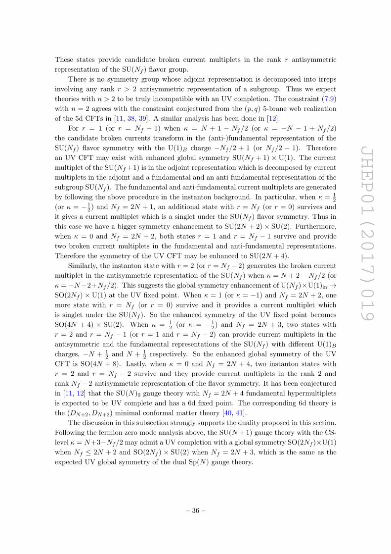
JHEP01(2017)019

These states provide candidate broken current multiplets in the rank r antisymmetric

representation of the SU(Nf ) flavor group.

There is no symmetry group whose adjoint representation is decomposed into irreps

involving any rank r > 2 antisymmetric representation of a subgroup. Thus we expect

theories with n > 2 to be truly incompatible with an UV completion. The constraint (7.9)

with n = 2 agrees with the constraint conjectured from the (p, q) 5-brane web realization

of the 5d CFTs in [11, 38, 39]. A similar analysis has been done in [12].

For r = 1 (or r = Nf − 1) when κ = N + 1 − Nf/2 (or κ = −N − 1 + Nf/2)

the candidate broken currents transform in the (anti-)fundamental representation of the

SU(Nf ) flavor symmetry with the U(1)B charge −Nf/2 + 1 (or Nf/2 − 1). Therefore

an UV CFT may exist with enhanced global symmetry SU(Nf + 1) × U(1). The current

multiplet of the SU(Nf +1) is in the adjoint representation which is decomposed by current

multiplets in the adjoint and a fundamental and an anti-fundamental representation of the

subgroup SU(Nf ). The fundamental and anti-fundamental current multiplets are generated

by following the above procedure in the instanton background. In particular, when κ = 12

(or κ = −12) and Nf = 2N + 1, an additional state with r = Nf (or r = 0) survives and

it gives a current multiplet which is a singlet under the SU(Nf ) flavor symmetry. Thus in

this case we have a bigger symmetry enhancement to SU(2N + 2)× SU(2). Furthermore,

when κ = 0 and Nf = 2N + 2, both states r = 1 and r = Nf − 1 survive and provide

two broken current multiplets in the fundamental and anti-fundamental representations.

Therefore the symmetry of the UV CFT may be enhanced to SU(2N + 4).

Similarly, the instanton state with r = 2 (or r = Nf − 2) generates the broken current

multiplet in the antisymmetric representation of the SU(Nf ) when κ = N + 2−Nf/2 (or

κ = −N−2+Nf/2). This suggests the global symmetry enhancement of U(Nf )×U(1)in →SO(2Nf ) × U(1) at the UV fixed point. When κ = 1 (or κ = −1) and Nf = 2N + 2, one

more state with r = Nf (or r = 0) survive and it provides a current multiplet which

is singlet under the SU(Nf ). So the enhanced symmetry of the UV fixed point becomes

SO(4N + 4) × SU(2). When κ = 12 (or κ = −1

2) and Nf = 2N + 3, two states with

r = 2 and r = Nf − 1 (or r = 1 and r = Nf − 2) can provide current multiplets in the

antisymmetric and the fundamental representations of the SU(Nf ) with different U(1)Bcharges, −N + 1

2 and N + 12 respectively. So the enhanced global symmetry of the UV

CFT is SO(4N + 8). Lastly, when κ = 0 and Nf = 2N + 4, two instanton states with

r = 2 and r = Nf − 2 survive and they provide current multiplets in the rank 2 and

rank Nf − 2 antisymmetric representation of the flavor symmetry. It has been conjectured

in [11, 12] that the SU(N)0 gauge theory with Nf = 2N + 4 fundamental hypermultiplets

is expected to be UV complete and has a 6d fixed point. The corresponding 6d theory is

the (DN+2, DN+2) minimal conformal matter theory [40, 41].

The discussion in this subsection strongly supports the duality proposed in this section.

Following the fermion zero mode analysis above, the SU(N + 1) gauge theory with the CS-

level κ = N+3−Nf/2 may admit a UV completion with a global symmetry SO(2Nf )×U(1)

when Nf ≤ 2N + 2 and SO(2Nf ) × SU(2) when Nf = 2N + 3, which is the same as the

expected UV global symmetry of the dual Sp(N) gauge theory.

– 36 –

JHEP01(2017)019

Nf SU(N)±(N+1−Nf/2) Nf SU(N)±(N+2−Nf/2)

≤ 2N SU(Nf + 1)×U(1) ≤ 2N + 1 SO(2Nf )×U(1)

2N + 1 SU(Nf + 1)× SU(2) 2N + 2 SO(2Nf )× SU(2)

2N + 2 SU(Nf + 2) 2N + 3 SO(2Nf + 2)

Table 1. Enhanced global symmetries of the 5d SCFTs. See also [11, 12].

7.2 From Sp(N) to exotic SU(N + 1)

We first discuss the superconformal index and the instanton partition function of Sp(N)

gauge theory. The superconformal index of the Sp(N) gauge theory with Nf fundamental

flavors takes the form

IN,Nf

Sp (wa,qSp;p,q) =(IV )N

N !

·∮ N∏i=1

dzi2πizi

∣∣∣∣∣∏Ni>j(z

±i z±j ;p,q)∞

∏Ni=1(z±2

i ;p,q)∞∏Ni=1

∏Nf

a=1(√pqz±i /wa;p,q)∞

ZN,Nf

Sp,inst(zi,wa,qSp;p,q)

∣∣∣∣∣2

.

(7.12)

The function ZN,Nf

Sp,inst is the instanton partition function of Sp(N) gauge theory, which

can be computed using localization of the path integral on the instanton moduli space

given in [30, 42]. The 5d Sp(N) instanton partition functions are studied in great detail

in [6, 26]. The results are summarized in appendix A.

The Sp(N) gauge theory has O(k) dual gauge group in the ADHM quantum mechanics.

At each instanton sector we will compute two partition functions Z+k and Z−k for O(k)+

and O(k)−, respectively,

Z±k (α,m; ε1,2) =1

|W |

∮ n∏I=1

dφI2πi

Z±vec(φ, α; ε1,2)

Nf∏a=1

Z±fund(φ, α,ma; ε1,2) , (7.13)

with k = 2n + χ and χ = 0 or 1. See appendix A.2 for details. In the following, we will

assume that θ = 0 for odd N + Nf and θ = π for even N + Nf while choosing the same

mass signs for all matter fields for notational convenience.

The k instanton partition function can be written as

ZkSp(odd)(α,m; ε1,2) =1

2

[Z+k (α,m; ε1,2) + Z−k (α,m; ε1,2)

],

ZkSp(even)(α,m; ε1,2) =(−1)k

2

[Z+k (α,m; ε1,2)− Z−k (α,m; ε1,2)

]. (7.14)

For instance, when k = 1, there is no integral and the instanton partition function is simply

given by sum of two partition functions

Z+k=1 =

p3/2q3/2∏Nf

a=1w−1/2a (−1 + wa)

(1− p)(1− q)∏Ni=1(1−√pqz±i )

, Z−k=1 =p3/2q3/2

∏Nf

a=1w−1/2a (1 + wa)

(1− p)(1− q)∏Ni=1(1 +

√pqz±i )

,

(7.15)

for O(1)+ and O(1)−, respectively.

– 37 –

JHEP01(2017)019

For higher instantons, we need to evaluate the contour integral over O(k) Coulomb

branch parameters using the JK-residue prescription. For example, the 2-instanton parti-

tion function has a contour integral over one variable φ1 for O(2)+ sector, whereas has no

integral for O(2)− sector. The JK-prescription tells us that the poles we should pick up are

φ1 ± αi + ε+ = 0 , 2φ1 + ε1 = 0 , 2φ1 + ε2 = 0 , (‘0’ ≡ 0 mod 2π) . (7.16)

The sum over the JK-residues plus the O(2)− contribution gives the full 2-instanton par-

tition function.

Furthermore, when Nf = 2N + 4, there exists a continuum in the instanton quantum

mechanics associated to a classical noncompact Coulomb branch. The partition function

involves an extra contribution coming from this continuum which should be removed to

obtain the correct QFT partition function. We find that the extra contribution takes

the form

ZNf=8Sp,extra = PE

[− 1 + pq

2(1− p)(1− q)q2

Sp

]. (7.17)

The half-integral coefficient in the letter index obviously shows that this is coming from

a continuum. This correction factor can also be obtained by taking a half of the residue

at infinity φI = ±∞ in the integral formula. The QFT instanton partition function is

therefore defined as

ZN,Nf=8Sp,inst = Z

N,Nf=8Sp,QM /Z

Nf=8Sp,extra , (7.18)

where ZSp,QM is the standard instanton partition function before removing the extra factor.

Next, we need to assemble the instanton partition function and 1-loop determinants

into the hemisphere partition function for Dirichlet boundary conditions:

IIN,Nf

Sp (zi, wa, qSp; p, q) =

∏Ni>j(pqz

±i z±j )∞

∏Ni=1(pqz±2

i ; p, q)∞∏Ni=1

∏Nf

a=1(√pqz±i /wa; p, q)∞

ZN,Nf

Sp,inst(zi, wa, qSp; p, q) .

(7.19)

The hemisphere index for the SU(N +1) theory is similarly defined and takes the form

IIN+1,Nf

SU (zi, wa, qSU; p, q) =

∏N+1i 6=j (pqzi/zj ; p, q)∞∏N+1

i=1

∏Nf

a=1(√pqzi/wa; p, q)∞

ZN+1,Nf

SU,inst (zi, wa, qSU; p, q) .

(7.20)

with an a-priory unknown instanton contribution ZN+1,Nf

SU,inst .

The degrees of freedom on the duality wall have the 4d index contribution∏N+1i=1

∏Nj=1 Γ(

√λz′iz

±j )∏N+1

i>j Γ(λz′iz′j)

, (7.21)

where z′ and z are the fugacities for the bulk SU(N + 1) and Sp(N) gauge groups. To

couple this to the 5d index, we need to multiply the 4d Sp(N) vector multiplet contribution

and integrate the Sp(N) gauge fugacities z. The result is given by

DIIN,Nf

Sp =

∮dµzi∆

(C)(z, z′, λ)IIN,Nf

Sp (zi, qSp, wa) , (7.22)

– 38 –

JHEP01(2017)019

where wa is the fugacity for U(Nf ) ⊂ SO(2Nf ) flavor symmetry and

∆(C)(z, z′, λ) =INV∏N+1i=1

∏Nj=1 Γ(

√λz′iz

±j )∏N+1

i>j Γ(λz′iz′j)∏Ni>j Γ(z±i z

±j )∏Ni=1 Γ(z±2

i ). (7.23)

Our conjecture is that the duality action D on the hemisphere index of the Sp(N)

gauge theory converts it into the hemisphere index of the SU(N + 1) gauge theory in the

other side of the wall. So the following relation is expected to hold

DIIN,Nf

Sp (zi, wa, qSp; p, q) = IIN+1,Nf

SU (z′i, w′a, qSU; p, q) . (7.24)

In this relation, the fugacities for the global symmetry in two sides of the wall should be

identified as

wa = λ1/2w′a , qSp = λ(N+1)/2

Nf∏a=1

(wa)−1/2 , qSU = λ−1

Nf∏a=1

(w′a)−1/2 . (7.25)

The first relation comes from the the constraint of the 4d superpotential. We deter-

mined the second and the third relations experimentally from the duality relations (7.24)

and (7.29), but they agree with the relations expected from cancellation of the mixed

’t Hooft anomalies for the duality wall.

The simplest example would be the duality action between Sp(2) and SU(3) gauge

theories with Nf flavors. To evaluate the integral in (7.24) and see the duality relation,

we should choose a particular contour. We take the contour to be along a unit circle while

assuming x� λ < 1.

Acting with the duality wall, we find the following result for Nf = 0:

DII2,0Sp (zi, qSp) ≡ II3,0

SU (zi, qSU) (7.26)

= 1 +(−χSU(3)

8 + χSU(3)3 qSU

)(x2 + χ

SU(2)2 (y)x3 + χ

SU(2)3 (y)x4

)+(χ

SU(3)8 + χ

SU(3)10 + χ

SU(3)

10−(χ

SU(3)3 + χ

SU(3)15

)qSU + χ

SU(3)6 q2

SU

)x4 +O(x5)

where χSU(3)r is the SU(3) character of the dimension r irrep with fugacities zi. We checked

that the right hand side agrees with the perturbative part of the SU(3) hemisphere index

and admits an expansion in non-negative powers of qSU, up to the order x5.

For general Nf ≤ 8, we find

DII2,Nf

Sp (zi,wa,qSp) ≡ II3,Nf

SU (zi,w′a,qSU) (7.27)

= 1+χSU(3)3 χ

U(Nf )x+

[−χSU(3)

8 (z)+χSU(3)6 χ

U(Nf )+χ

SU(3)

3χ

U(Nf )

Λ2

+χSU(2)2 (y)χ

SU(3)3 χ

U(Nf )+(χ

SU(3)3 +χ

U(Nf )

Λ2+χ

U(Nf )

Λ8

)Nf∏a=1

√w′aqSU

]x2+O(x3),

where χU(Nf )Y is the U(Nf ) character with fugacities (w′a)

−1 of a irrep labeled by a Young

tableau Y . We have identified the parameters as (7.25). The perturbative part on the

– 39 –

JHEP01(2017)019

right hand side agrees with that of the SU(3) theory and the other parts are expanded by

non-negative powers of qSU. This relation has been checked at least up to x3 order.

In appendix B, we shall suggest a UV prescription of the instanton moduli space of our

exotic SU(3) theory with matter fields, whose partition function precisely reproduces the

right hand side. In addition, we will explicitly compute the superconformal index of this

SU(3) theory and show the desired global symmetry enhancement at the UV fixed point.

One can also consider the generalization to higher rank gauge theories. Acting with

the duality wall on the hemisphere index of the Sp(3) theories, we obtain

DII3,Nf≤3Sp (zi, wa, qSp) ≡ II4,Nf≤3

SU (zi, w′a, qSU) (7.28)

= 1+χSU(4)4 χ

U(Nf )x+

[−χSU(4)

15 +(χ

SU(4)4

)2

χU(Nf )

Λ2+χ

SU(4)10 χ

U(Nf )((w′)−2)

+χSU(2)2 (y)χ

SU(4)4 χ

U(Nf )+(χ

SU(4)6 (z)+χ

U(Nf )

Λ2

) Nf∏a=1

√waqSU

]x2+O(x3) .

for Nf ≤ 3, by identifying the parameters as (7.25). We checked that the right hand side

agrees with the perturbative part of the SU(4) hemisphere index and admits an expansion

in non-negative powers of qSU, at least up to the order x4.

Of course, the duality wall can also act in the opposite direction, from SU(N + 1)

to Sp(N).

DIIN+1,Nf

SU (z′, w′a, qSU) ≡∮dµz′∆

(A)(z′, z, λ)IIN+1,Nf

SU (z′i, w′a, qSU) = II

N,Nf

Sp (zi, wa, qSp) ,

(7.29)

where the 4d index of the boundary degrees of freedom involving the 4d vector multiplet

is given by

∆(A)(z′, z, λ) =INV∏Ni=1

∏N+1j=1 Γ(

√λ−1z±i /z

′j)∏N+1

i 6=j Γ(z′i/z′j)∏N+1i>j Γ(λ−1(z′iz

′j)−1)

. (7.30)

The contour is chosen along the unit circle with an assumption x � λ−1 < 1 and the

parameters are matched as (7.25).

Of course, this follows from the CA and AC inversion formula introduced in [10]:∮dµz′∆

(A)(z′, x, λ)

∮dµz∆

(C)(z, z′, λ)f(z) = f(x) ,∮dµz∆

(C)(z, x, λ)

∮dµz′∆

(A)(z′, z, λ)f(z′) = f(x) . (7.31)

Note that the contours should be chosen along unit circles by assuming x � λ−1 < 1

for the A-type integral, but by assuming x � λ < 1 for the C-type integral as specified

already.

7.3 Wilson loops

In this subsection, we will study the properties of BPS Wilson loops under the conjectural

duality in the previous sections. We will focus on the simplest cases: fundamental Wilson

– 40 –

JHEP01(2017)019

loops of the Sp(2) and SU(3) gauge theories meeting at the interface. The Wilson loops on

two sides of the wall are connected at the boundary by the bi-fundamental chiral multiplet

q. The chiral multiplet q has charge 12 under the non-anomalous U(1)λ global symmetry.

To cancel the global charge when it couples to the Wilson loops, we combine the gauge

Wilson loops with a flavor Wilson loop for the U(1)λ, with flavor charge 12 , which follows

from the similar argument in section 4. We will compute hemisphere indices and test this

duality property between two fundamental Wilson loops.

We first compute the hemisphere indices with fundamental Wilson loops inserted at the

origin. We need to compute the instanton partition function in the presence of Wilson loops.

As explained in section 4, Wilson loops are represented by equivariant Chern characters

in the localization, and that for the fundamental Wilson loop is given in (A.13). Then the

localized partition function can be written in terms of the equivariant Chern characters as

in (4.1).

For the Sp(N) gauge theory, the equivariant Chern character for the fundamental

Wilson loop can be written, at k-instantons, as

Ch+fund(eα, eφ) =

N∑i=1

(eαi + e−αi)− (1− p)(1− q)(pq)−1/2n∑I=1

(eφI + e−φI + χ) , (7.32)

Ch−fund(eα, eφ) =

N∑i=1

(eαi + e−αi)− (1− p)(1− q)(pq)−1/2n∑I=1

(eφI + e−φI + eiπχ) ,

with k = 2n + χ and χ = 0 or 1. Here the superscripts ± means those for O(k)± sectors.

Then the 1-instanton partition function can be written as

W+k=1 =

(pq)3/2(∑N

i=1(eαi + e−αi)− (1− p)(1− q)(pq)−1/2)∏Nf

a=1 2 sinh ma2

(1− p)(1− q)∏Ni=1(1−√pqe±αi)

,

W−k=1 =(pq)3/2

(∑Ni=1(eαi + e−αi) + (1− p)(1− q)(pq)−1/2

)∏Nf

a=1 2 cos ma2

(1− p)(1− q)∏Ni=1(1 +

√pqe±αi)

. (7.33)

There could be extra instanton corrections to the Wilson loop index as we have seen in

section 4. For the cases in this section, however, we find that there is no such corrections

up to certain order in x expansion.

Now we consider the duality wall action on the hemisphere index of the Sp(N) theory

with the fundamental Wilson loop. We propose that the fundamental Wilson loop partition

function of the Sp(N) theory is mapped to that of the SU(N + 1) theory after passing

through the duality wall as follows:

DWSp(N),Nf

fund (zi, wa, λ) = λ1/2WSU(N+1),Nf

fund (zi, w′a, λ−1) , (7.34)

with the parameter identification in (7.25). The duality action D is defined in the same way

as in (7.22), but the hemisphere indices IIN,Nf

Sp,SU in both sides are replaced by the Wilson

loop indices WN,Nf

Sp,SU. The prefactor λ1/2 is due to the U(1)λ flavor Wilson loop.

– 41 –

JHEP01(2017)019

We compute the hemisphere indices of the Sp(2) gauge theories and test this duality.

We obtain

DWSp(2),0fund (zi, qSp) ≡ λ1/2W

SU(3),1fund (zi, qSU) (7.35)

= χSU(3)3 (z)+

(−χSU(3)

15 (z)−χSU(3)

3(z)2+χ

SU(3)6 qSU

)x2

+χSU(2)2 (y)χ

SU(3)3 (z)x3+χ

SU(2)2 (y)χ

SU(3)3 (z)2

(−χSU(3)

3(z)+qSU

)x3+O(x4) ,

for Nf = 0, and

DWSp(2),1fund (zi,w,qSp)≡λ1/2W

SU(3),1fund (zi,w

′,qSU)

=χSU(3)3 (z)+

((w′1)−1χ

SU(3)3 (z)2+(w′1)−1/2qSU

)x+(−χSU(3)

15 (z)−χSU(3)

3(z)2

)x2

+(

(w′1)−2χSU(3)10 (z)+(w′1)−2χ

SU(3)8 (z)+(w′1)−1χ

SU(2)2 (y)χ

SU(3)3 (z)2

)x2

+(χ

SU(3)6 (z)+(w′1)−2χ

SU(3)3 (z)

)(w′1)1/2qSUx

2+O(x3), (7.36)

for Nf = 1. We have checked that, for each Nf = 0, 1 case, the right hand side admits an

expansion in non-negative powers of qSU and the perturbative part agrees with that of the

SU(3) gauge theory, up to x4 order. It also turns out that the right hand sides agree up to

x4 order with the hemisphere indices of the SU(3) theories with the fundamental Wilson

loop whose instanton partition functions are computed using the UV prescription given in

appendix B.

Acknowledgments

The research of DG and HK was supported by the Perimeter Institute for Theoretical

Physics. Research at Perimeter Institute is supported by the Government of Canada

through Industry Canada and by the Province of Ontario through the Ministry of Eco-

nomic Development and Innovation.

A 5d Nekrasov’s instanton partition function

The moduli space of instantons has complicated singularities which are associated to one or

more instantons shrinking to zero size. In the context of five-dimensional supersymmetric

gauge theories, these field configurations are outside the obvious regime of validity of the

gauge theory description of the theory. Correspondingly, the definition of the gauge the-

ory instanton partition functions through equivariant localization on the instanton moduli

spaces requires a prescription of how to deal with the singularities, which will depend on a

choice of UV completion of the gauge theory.

It is very challenging to work directly on the singular moduli spaces. Even in the

absence of extra matter fields this was done only recently [43] using the technology of

equivariant intersection cohomology. Extra matter fields, in the form of hypermultiplets

transforming in some representation of the gauge group, provide additional fermion zero

– 42 –

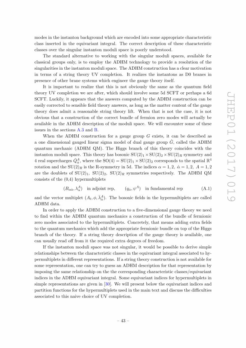
JHEP01(2017)019

modes in the instanton background which are encoded into some appropriate characteristic

class inserted in the equivariant integral. The correct description of these characteristic

classes over the singular instanton moduli space is poorly understood.

The standard alternative to working with the singular moduli spaces, available for

classical groups only, is to employ the ADHM technology to provide a resolution of the

singularities in the instanton moduli space. The ADHM construction has a clear motivation

in terms of a string theory UV completion. It realizes the instantons as D0 branes in

presence of other brane systems which engineer the gauge theory itself.

It is important to realize that this is not obviously the same as the quantum field

theory UV completion we are after, which should involve some 5d SCFT or perhaps a 6d

SCFT. Luckily, it appears that the answers computed by the ADHM construction can be

easily corrected to sensible field theory answers, as long as the matter content of the gauge

theory does admit a reasonable string theory lift. When that is not the case, it is not

obvious that a construction of the correct bundle of fermion zero modes will actually be

available in the ADHM description of the moduli space. We will encounter some of these

issues in the sections A.3 and B.

When the ADHM construction for a gauge group G exists, it can be described as

a one dimensional gauged linear sigma model of dual gauge group G, called the ADHM

quantum mechanic (ADHM QM). The Higgs branch of this theory coincides with the

instanton moduli space. This theory has bosonic SU(2)1×SU(2)2×SU(2)R symmetry and

4 real supercharges QAα , where the SO(4) = SU(2)1× SU(2)2 corresponds to the spatial R4

rotation and the SU(2)R is the R-symmetry in 5d. The indices α = 1, 2, α = 1, 2, A = 1, 2

are the doublets of SU(2)1, SU(2)2, SU(2)R symmetries respectively. The ADHM QM

consists of the (0,4) hypermultiplets

(Bαα, λAα ) in adjoint rep, (qα, ψ

A) in fundamental rep (A.1)

and the vector multiplet (At, φ, λAα ). The bosonic fields in the hypermultiplets are called

ADHM data.

In order to apply the ADHM construction to a five-dimensional gauge theory we need

to find within the ADHM quantum mechanics a construction of the bundle of fermionic

zero modes associated to the hypermultiplets. Concretely, that means adding extra fields

to the quantum mechanics which add the appropriate fermionic bundle on top of the Higgs

branch of the theory. If a string theory description of the gauge theory is available, one

can usually read off from it the required extra degrees of freedom.

If the instanton moduli space was not singular, it would be possible to derive simple

relationships between the characteristic classes in the equivariant integral associated to hy-

permultiplets in different representations. If a string theory construction is not available for

some representation, one can try to guess an ADHM description for that representation by

imposing the same relationship on the the corresponding characteristic classes/equivariant

indices in the ADHM equivariant integral. Some equivariant indices for hypermultiplets in

simple representations are given in [30]. We will present below the equivariant indices and

partition functions for the hypermultiplets used in the main text and discuss the difficulties

associated to this naive choice of UV completion.

– 43 –

JHEP01(2017)019

The instanton partition function takes the form of the instanton series expansion as

Zinst =∞∑k=0

qkZk , (A.2)

with an instanton counting parameter q. The Zk is the k instanton partition function. It

is the supersymmetric Witten index of the 1d ADHM QM. It also admits a path integral

representation. The supersymmetric localization was employed to evaluate this path in-

tegral of the ADHM quantum mechanics in [18, 23]. See also [26–28] for 1d localization

calculations. We will now summarize some results.

A.1 SU(N) partition function

The ADHM quantum mechanics has dual gauge group G = U(k) for k instantons. In the

bulk 5d theory, one can also turn on a classical CS coupling κ when N ≥ 3. It induces a

Chern-Simons coupling in the 1d quantum mechanics [44, 45].

κ

∫dtTr(At − φ) . (A.3)

The k instanton partition function takes the following integral expression

Zk(α,m; ε1,2) =1

k!

∮ k∏I=1

dφI2πi

e−κ∑k

I=1 φIZvec(φ, α; ε1,2)∏a

ZRa(φ, α,ma; ε1,2) , (A.4)

where ZkRais the contribution from a hypermultiplet in Ra representation and ma is the

mass parameter. We will often use fugacities zi ≡ eαi , wa ≡ ema . The vector multiplet

factor is

Zvec(φ, α; ε1,2) =

∏kI 6=J 2 sinh φI−φJ

2

∏kI,J 2 sinh φI−φJ+2ε+

2∏kI,J 2 sinh φI−φJ+ε1

2 2 sinh φI−φJ+ε22

∏Ni=1

∏kI=1 2 sinh ±(φI−αi)+ε+

2

.

(A.5)

The hypermultiplet factor will be discussed later.

We still have the contour integral to be evaluated. The contour integral of the instan-

ton partition function should be performed using the Jeffrey-Kirwan method [26]. If the

hypermultiplet factor has only fermionic contributions, as our naive expectation from the

zero mode analysis in the 5d QFT, we need to take into account only the vector multiplet

factor. The JK-prescription tells us that the residue sum of the following poles will give

the final result.

φI − αi + ε+ = 0 , φI − φJ + ε1 = 0 , φI − φJ + ε2 = 0 , (A.6)

with I > J . However, we will see that the hypermultiplets can introduce extra bosonic

degrees for the UV completion of their zero modes. Thus they can also provide nontrivial

JK-poles above the poles from the vector multiplet. We will discuss some examples below.

– 44 –

JHEP01(2017)019

A.2 Sp(N) partition function

For Sp(N) gauge theory, the ADHM quantum mechanics has G = O(k) dual gauge group.

Since the O(k) group has two disconnected components O(k)+ and O(k)−, we will get two

partition functions Z+k and Z−k at each instanton sector. The k instanton partition function

is then given by a sum of these two functions. In addition, the Sp(N) gauge theory has a

Z2 valued θ angle associated with π4 (Sp(N)) = Z2 [3]. Two possible θ parameters lead to

the following two different combinations [7, 46]:

ZSpk =

12(Z+

k + Z−k ) , θ = 0

(−1)k

2 (Z+k − Z

−k ) , θ = π

. (A.7)

When the theory couples to more than one fundamental hypermultiplet, the θ angle be-

comes unphysical because it can be effectively absorbed by flipping the sign of a single

mass of one fundamental matter.

The k instanton partition function takes the form

Z±k (α,m; ε1,2) =1

|W |

∮ n∏I=1

dφI2πi

Z±vec(φ, α; ε1,2)∏a

Z±Ra(φ, α,ma; ε1,2) , (A.8)

with k = 2n+ χ and χ = 0 or 1. The Weyl factor is given by

|W |χ=0+ =

1

2n−1n!, |W |χ=1

+ =1

2nn!, |W |χ=0

− =1

2n−1(n− 1)!, |W |χ=1

− =1

2nn!.

(A.9)

The vector multiplet for O(k)+ sector gives the contribution

Z+vec =

[1

2sinh±ε−+ε+2

∏Ni=12sinh±αi+ε+

2

n∏I=1

2sinh±φI

2 2sinh±φI+2ε+2

2sinh±φI±ε−+ε+2

]χ(A.10)

×n∏I=1

2sinhε+

2sinh±ε−+ε+2

∏Ni=12sinh±φI±αi+ε+

2

·∏nI>J2sinh±φI±φJ

2 2sinh±φI±φJ+2ε+2∏n

I=12sinh±2φI±ε−+ε+2

∏nI>J2sinh±φI±φJ±ε−+ε+

2

.

For O(k)− sector, the vector multiplet contribution is

Z−vec =1

2sinh±ε−+ε+2

∏Ni=12cosh±αi+ε+

2

n∏I=1

2cosh±φI

2 2cosh±φI+2ε+2

2cosh±φI±ε−+ε+2

(A.11)

×n∏I=1

2sinhε+

2sinh±ε−+ε+2

∏Ni=12sinh±φI±αi+ε+

2

·∏nI>J2sinh±φI±φJ

2 2sinh±φI±φJ+2ε+2∏n

I=12sinh±2φI±ε−+ε+2

∏nI>J2sinh±φI±φJ±ε−+ε+

2

,

with k = 2n+ 1 and

Z−vec =2coshε+

2sinh±ε−+ε+2 2sinh(±ε−+ε+)

∏Ni=12sinh(±αi+ε+)

n−1∏I=1

2sinh(±φI)2sinh(±φI+2ε+)

2sinh(±φI±ε−+ε+)(A.12)

×n−1∏I=1

2sinhε+

2sinh±ε−+ε+2

∏Ni=12sinh±φI±αi+ε+

2

·∏n−1I>J2sinh±φI±φJ

2 2sinh±φI±φJ+2ε+2∏n−1

I=1 2sinh±2φI±ε−+ε+2

∏n−1I>J2sinh±φI±φJ±ε−+ε+

2

,

with k = 2n.

– 45 –

JHEP01(2017)019

A.3 Hypermultiplets

A hypermultiplet develops fermion zero modes in the instanton background. The presence

of the fermion zero modes can be observed using an index theorem. Accordingly, it is

expected that the bulk hypermultiplets induce fermionic degrees on the instanton moduli

space. When we attempt to engineer an ADHM quantum mechanics description of these

fermionic zero modes on the Higgs branch, however, extra bosonic degrees of freedom are

in general required. Often these bosonic zero modes give rise to extra classical branches

of vacua in the ADHM quantum mechanics, or extra continuum contributions to the spec-

trum, which may be spurious from the point of view of the 5d gauge theory. In string

theory constructions, they may describe D0 branes moving away from the brane system

which engineers the 5d gauge theory. These spurious branches of vacua must be carefully

subtracted from the final answer.

We can give a few simple examples of this phenomenon. The instanton moduli space

of a 5d gauge theory with an adjoint hypermultiplet has a string theory embedding. The

instanton states can be interpreted as the D0/D4-brane bound states in this case. The

1d gauge theory living on the D0-branes is described by the ADHM quantum mechanics

with additional matter fields corresponding to the bulk adjoint hypermultipet. This theory

involves extra real 4 dimensional bosonic fields that parametrize the 4 transverse directions

to the D4-branes in which the 5d gauge theory supports. The non-commutativity parameter

(or FI parameter) in the 1d QM generally make these directions massive. However, when

the commutativity is restored, these branches of vacua open up D0-branes (or instantons)

can escape to infinity.

Similarly, the UV completion of instanton dynamics in Sp(N) gauge theory with an an-

tisymmetric and fundamental hypermultiplets has extra bosonic degrees of freedom from

the hypermultiplets. Its string theory embedding is given by D0-D4-D8-O8 brane sys-

tem [47]. The extra bosonic modes again parametrize the transverse directions to the

D4-branes. In particular, the ADHM for this theory does not have noncommutative defor-

mation of the space. Hence the observables computed using this UV completion in general

involves extra contributions to be subtracted off. One can find examples in [26].

Next, we can describe our guess for the contribution of hypermultiplets in tensor powers

of the fundamental representation, based on the prescription given in [30]. If we could ignore

the singularities, the hypermultiplets introduce vector bundles on the instanton moduli

space, and the vector bundles are constructed by tensor products of an universal bundle E .

The tensor product structure of the vector bundle inherits that of the representation of the

5d hypermultiplet. We will now pretend that the same prescription can be applied to the

ADHM-resolved moduli space of instantons. In [30], it was suggested that the equivariant

index for the hypermultiplet can be computed by taking tensor product of the equivariant

Chern character of the bundle E , which is given by [30, 48]

ChE(eα, eφ; p, q) = χfund(eαi)− (1− p)(1− q)(pq)−1/2χfund(eφI ) , (A.13)

where χfund(eαi) and χfund(eφI ) denote the character of the fundamental representations of

the guage group G and the dual gauge group G, respectively. For example, the equivariant

– 46 –

JHEP01(2017)019

indices for the hypermultiplets in the fundamental, symmetric, antisymmetric and adjoint

representations are given by, respectively,

indfund(eα, eφ; p, q) =

√pq

(1− p)(1− q)ChE(e

α, eφ; p, q) ,

indsym(eα, eφ; p, q) =

√pq

(1− p)(1− q)ChE⊗E(e

α, eφ; p, q) ,

indanti(eα, eφ; p, q) =

√pq

(1− p)(1− q)Ch∧2E(e

α, eφ; p, q) ,

indadj(eα, eφ; p, q) =

√pq

(1− p)(1− q)ChE⊗E∗(e

α, eφ; p, q) . (A.14)

where the tensor product of the Chern character is defined using the usual tensor product

rule as

ChE⊗E(eα, eφ; p, q) =

1

2

[ChE(e

α, eφ; p, q)2 + ChE(e2α, e2φ; p2, q2)

],

Ch∧2E(eα, eφ; p, q) =

1

2

[ChE(e

α, eφ; p, q)2 − ChE(e2α, e2φ; p2, q2)],

ChE⊗E∗(eα, eφ; p, q) = ChE(e

α, eφ; p, q)× ChE(e−α, e−φ; p−1, q−1) . (A.15)

The equivariant indices in other representations can be obtained in the similar manner.

The resulting index computed in this way contains terms independent of the fugacity eφI

for G. These terms amount to the perturbative contribution, so we will ignore them when

we compute the instanton partition function.

The contribution to the instanton partition function of the hypermultiplets can be

easily obtained using the relevant equivariant indices. There is a conversion rule for 5d

calculation

indR =∑i

niezi → ZR =

∏i

[2 sinh

zi2

]ni

. (A.16)

Thus the plethystic exponential of the equivariant index yields the instanton partition

function contribution of the hypermultiplet. One can check that the contribution from

an adjoint hypermultiplet computed using this prescription agrees with that from the

localization of the ADHM quantum mechanics in [49].

Let us present explicit expressions for the hypermultiplets discussed in the main con-

text. For SU(N) gauge theory, the fundamental hypermultiplet contribution is

Zfund =

k∏I=1

2 sinhφI −m

2, (A.17)

with a mass parameter m. The antisymmetric hyper has the following contribution

Zasym =

∏Ni=1

∏kI=12sinhφI+αi−m

2

∏kI>J2sinhφI+φJ−m−ε−

2 2sinh−φI−φJ+m−ε−2∏k

I>J2sinhφI+φJ−m−ε+2 2sinh−φI−φJ+m−ε+

2

∏kI=12sinh2φI−m−ε+

2 2sinh−2φI+m−ε+2

.

(A.18)

– 47 –

JHEP01(2017)019

For Sp(N) gauge theory, the fundamental representation has the contribution

Z+fund =

(2 sinh

m

2

)χ n∏I=1

2 sinh±φI +m

2, (A.19)

for O(k)+, and

Z−fund = 2 coshm

2

n∏I=1

2 sinh±φI +m

2, (A.20)

for O(k)− with k = 2n+ 1, and

Z−fund = 2 sinhm

2

n−1∏I=1

2 sinh±φI +m

2, (A.21)

for O(k)− with k = 2n. These are read off from the corresponding equivariant indices

in (A.14).

Next, we can assemble a modification of the bare ADHM quantum mechanics which

would reproduce these modifications to the equivariant integrand. The contribution for

the fundamental hypermultiplet implies that a fundamental matter induces a (0, 4) fermi

multiplet in fundamental representation of G in the ADHM QM. This agrees with our

expectation that the hypermultiplet develops fermion zero modes in the instanton back-

ground. On the other hand, the contribution from the antisymmetric hyper has factors

in denominator as well as the factors in numerator. The numerator factors correspond to

a fermi multiplet in the bifundamental representation of G × G and a conjugate pair of

fermi multiplets in the antisymmetric representation of G. While, the denominator factors

corresponds to a pair of (0, 4) hypermultiplets in the symmetric representation of G. This

means that the UV completion of the zero modes acquires nontrivial bosonic degrees which

are not present in the zero mode analysis of the 5d QFT.

The computation of the 1d equivariant integral requires both an integrand and a choice

of integration contour/prescription. The latter, in a sense, can be used to include or exclude

the contribution of certain classical branches of vacua, by selecting which poles should be

picked by the contour integral. The standard prescription in 1d localization computations

is the JK-prescription. To read the relevant poles from the JK-prescription, we should know

the exact representations of the extra bosonic degrees under G rotation. However, although

the recipe given in [30] and in this section allows us to know the matter contents in the

ADHM QM, it yet has an ambiguity in the exact representations of the multiplets. More

precisely, it cannot distinguish a certain complex representation R and its conjugation,

i.e. ‘sinh R(φ)+···2 ’ and ‘− sinh −R(φ)−···

2 ’. Since we could not resolve this issue, we will give

prescriptions for it case by case in the main context.

Further spurious contributions included by the standard JK-prescription have to be

removed on a case-by-case basis. See [26] for few examples.

B Partition functions of exotic SU(3) theory

In this appendix, we propose a prescription to compute the instanton partition functions

of the exotic SU(3) theories with matters. With these results, we compute the hemisphere

– 48 –

JHEP01(2017)019

indices and then show that they agree with the hemisphere indices obtained in section 7.2

using the duality wall action on the Sp(2) hemisphere indices.

We are interested in the SU(3) SQCD with κ = 5 − Nf/2, which obviously violates

the bound |κ| ≤ 3 − Nf/2 in [4]. As mentioned before, when the theory violates this

bound, the localization integral of the instanton partition function from the usual ADHM

quantum mechanics encounters higher degree poles at the infinities φI = ±∞. These poles

are associated to the classical Coulomb branch of vacua in the ADHM quantum mechanics

and not to the to the instanton moduli space which is described by the Higgs branch.

Unfortunately, we do not know how to remove these spurious contributions when the

degree of the pole is higher than 1. In what follows, we will explain how to avoid having

higher degree poles at infinity by introducing ‘pseudo’ hypermultiplets in the instanton

background. We will add two (or more) ‘pseudo’ hypermultiplets and integrate them out

at the end. This will allow us to evaluate the instanton partition function without having

the problem of the higher degree poles at infinity.

Let us first discuss the ‘pseudo’ hypermultiplet and the ADHM quantum mechanics.

The ‘pseudo’ hypermultiplet is simply the hypermultiplet in the antisymmetric representa-

tion of the SU(3). It should be equivalent to the fundamental hypermultiplet for the SU(3)

gauge theory. This is indeed the case for the perturbative analysis. However, the anti-

symmetric hypermultiplet affects the ADHM quantum mechanics in a different way from

that of the fundamental hypermultiplet. Strictly speaking, the ADHM quantum mechanics

is designed for the U(N) gauge theory since it involves singular U(1) instantons which is

regularized by introducing extra UV degrees of freedom. Therefore, fermion zero modes

from the antisymmetric hypermultiplet has a rather different UV completion than those

from the fundamental hypermultiplet in the ADHM QM.

The fermionic zero modes from the antisymmetric hypermultiplet provide many non-

trivial multiplets, not just fermi multiplets but possibly also hypermultiplets including

extra bosonic zero modes, in the ADHM QM as depicted in figure 16. The ADHM quantum

mechanics is the N = (0, 4) gauge theory of U(k) gauge group with SU(2)1 × SU(2)2 ×SU(2)R symmetry. See appendix A for details. We then add a bi-fundamental chiral

fermion (black dashed arrow) of U(k) and SU(3) groups, and a (0, 4) fermi multiplet (blue

dashed arrow), which is a doublet under the SU(2)1 and in the antisymmetric representation

of U(k), and a hypermultiplet (red solid arrow) in the symmetric representation of U(k).

This is equivalent to add to the instanton moduli space a vector bundle given by the

antisymmetric product of the universal bundle in the fundamental representation.

We consider the SU(3) gauge theory with two ‘pseudo’ hypermultiplets and Nf funda-

mental hypermultiplets. The k-instanton partition function from the ADHM QM can be

written as

ZNf

QM,k =(−1)3+Nf

k!

∮ k∏I=1

dφI2πi

e−κ∑k

I=1φIZkvec(α,φ;p,q)

Nf∏a=1

Zkfund(φ,ma;p,q)

2∏a=1

Zkasym(φ,ti;p,q)

(B.1)

where Zkvec, Zkfund, Z

kasym are given in (A.5), (A.17), (A.18), respectively. We will set the

classical CS-level κ = 4−Nf/2. One can easily see that the integral then has a simple pole

at infinity φI = −∞, which is now controllable.

– 49 –

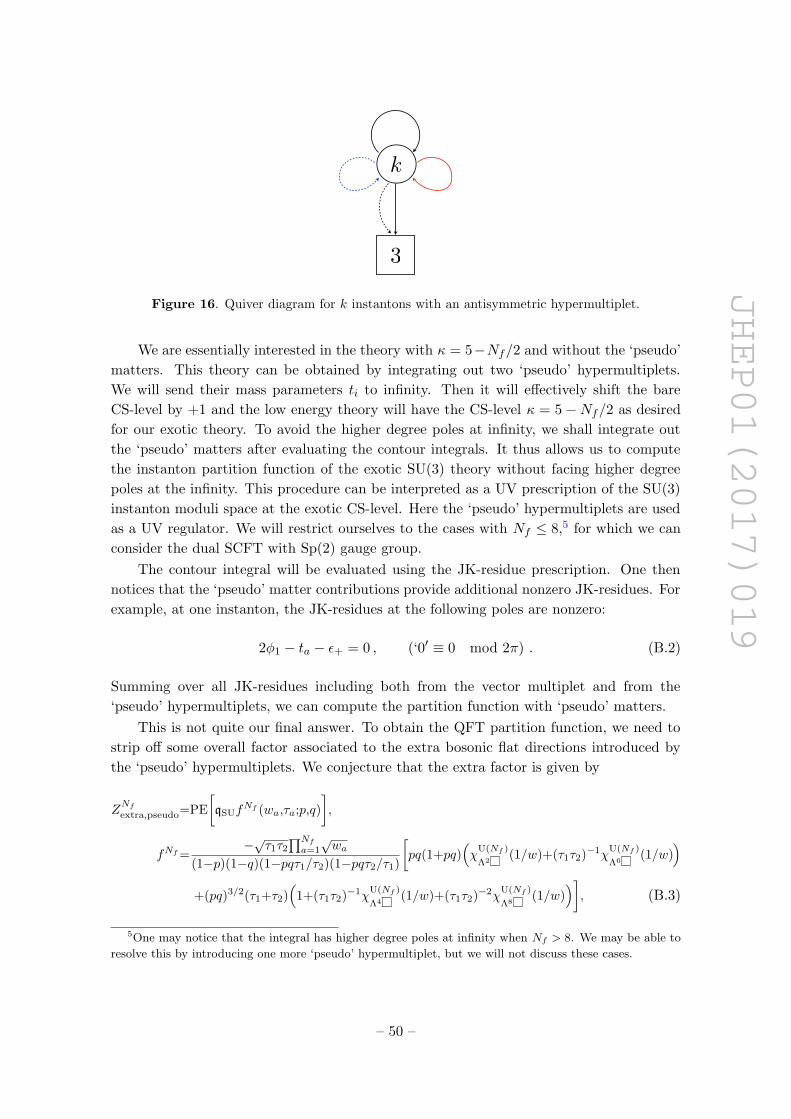
JHEP01(2017)019

k

3

Figure 16. Quiver diagram for k instantons with an antisymmetric hypermultiplet.

We are essentially interested in the theory with κ = 5−Nf/2 and without the ‘pseudo’

matters. This theory can be obtained by integrating out two ‘pseudo’ hypermultiplets.

We will send their mass parameters ti to infinity. Then it will effectively shift the bare

CS-level by +1 and the low energy theory will have the CS-level κ = 5−Nf/2 as desired

for our exotic theory. To avoid the higher degree poles at infinity, we shall integrate out

the ‘pseudo’ matters after evaluating the contour integrals. It thus allows us to compute

the instanton partition function of the exotic SU(3) theory without facing higher degree

poles at the infinity. This procedure can be interpreted as a UV prescription of the SU(3)

instanton moduli space at the exotic CS-level. Here the ‘pseudo’ hypermultiplets are used

as a UV regulator. We will restrict ourselves to the cases with Nf ≤ 8,5 for which we can

consider the dual SCFT with Sp(2) gauge group.

The contour integral will be evaluated using the JK-residue prescription. One then

notices that the ‘pseudo’ matter contributions provide additional nonzero JK-residues. For

example, at one instanton, the JK-residues at the following poles are nonzero:

2φ1 − ta − ε+ = 0 , (‘0′ ≡ 0 mod 2π) . (B.2)

Summing over all JK-residues including both from the vector multiplet and from the

‘pseudo’ hypermultiplets, we can compute the partition function with ‘pseudo’ matters.

This is not quite our final answer. To obtain the QFT partition function, we need to

strip off some overall factor associated to the extra bosonic flat directions introduced by

the ‘pseudo’ hypermultiplets. We conjecture that the extra factor is given by

ZNf

extra,pseudo=PE

[qSUf

Nf (wa,τa;p,q)

],

fNf =−√τ1τ2

∏Nf

a=1

√wa

(1−p)(1−q)(1−pqτ1/τ2)(1−pqτ2/τ1)

[pq(1+pq)

(χ

U(Nf )

Λ2(1/w)+(τ1τ2)−1χ

U(Nf )

Λ6(1/w)

)+(pq)3/2(τ1+τ2)

(1+(τ1τ2)−1χ

U(Nf )

Λ4(1/w)+(τ1τ2)−2χ

U(Nf )

Λ8(1/w)

)], (B.3)

5One may notice that the integral has higher degree poles at infinity when Nf > 8. We may be able to

resolve this by introducing one more ‘pseudo’ hypermultiplet, but we will not discuss these cases.

– 50 –

JHEP01(2017)019

where τa ≡ e−ta and χU(Nf )

ΛL is the character of the rank L antisymmetric irrep of the

U(Nf ) flavor group with fugacities 1/wa. For example, χU(Nf )

Λ2 (1/w) =∑Nf

a>b(wawb)−1.

Note that this extra factor is independent of the SU(3) gauge fugacities and thus it indeed

corresponds to the degrees of freedom decoupled from the 5d QFT. We have checked that,

after subtracting off this factor, the instanton partition function has no poles for τa and is a

finite polynomial in τ1 and τ2, as expected, at 1-instanton for all Nf and up to 2-instantons

for Nf < 6.

There is the usual correction factor coming from the continuum along the noncompact

Coulomb branch. It is associated to the residues at infinity φI = ±∞. We obtain

ZNf

extra,cont = PE

[−

qSU∏Nf

a=1

√wa

(1− p)(1− q)√τ1τ2

],

ZNf=8extra,cont = PE

[− qSU

(1− p)(1− q)

(√τ1τ2

−18∏

a=1

√wa + pq

√τ1τ2

8∏a=1

√wa−1

)]. (B.4)

The ‘correct’ partition function can then be written as

ZNf

inst(zi, wa, τa, qSU; p, q) = ZNf

QM/ZNf

extra , (ZNf

extra ≡ ZNf

extra,cont · ZNf

extra,pesudo) . (B.5)

where ZQM is the partition function of the ADHM QM evaluated with the JK-prescription.

We now integrate out the ‘pseudo’ hypers. We will send their masses to infinity ta →−∞,6 and take the leading contribution. By rescaling the instanton fugacity as qSU

√τ1τ2 →

qSU, we will end up with the instanton partition function of the SU(3) theory with Nf

flavors and the CS-level κ = 5−Nf/2:

Z3,Nf

inst (zi, wa, qSU; p, q) ≡ limτ1,τ2→∞

ZNf

inst(zi, wa, τa, qSU/√τ1τ2; p, q) . (B.6)

Taking into account the extra factors carefully, we compute 1-instanton partition func-

tions for Nf ≤ 8 and obtain

Z3,Nf

inst,k=1 =(χ

SU(3)3 (z) + χ

U(Nf )

Λ2 + χU(Nf )

Λ8

)(x2 + χ

SU(2)2 (y)x3 + χ

SU(2)3 (y)x4

)+(χ

U(Nf )

Λ5 − χSU(3)

3(z)χ

U(Nf ))(

x3 + χSU(2)2 (y)x4

)+(χ

SU(3)

6(z)− χSU(3)

3(z)χ

U(Nf )

Λ4 − χSU(3)3 (z)χ

U(Nf )

Λ6

)x4 +O(x5) . (B.7)

Combining the 1-loop determinant, we have checked that the hemisphere index of our exotic

SU(3) theory yields exactly the right hand side of the duality relation (7.27) between the

Sp(2) and SU(3) theories, in all examples at least up to x3 order. This result supports the

UV prescription of the exotic SU(3) theory in this section.

Similarly, we can compute the Wilson loop index of the exotic SU(3) theories using the

above UV prescription. An Wilson loop in a representation R inserts the corresponding

6We can also take the limit ta →∞. Then we will get the theory with CS-level κ = 3−Nf/2.

– 51 –

JHEP01(2017)019

equivariant Chern character into contour integral of the instanton partition function. At k-

instantons, the Wilson loop index before integrating out the pseudo hypers can be written as

WNf

QM,k =(−1)3+Nf

k!

∮ k∏I=1

dφI2πi

ChR(α,φ)·e−κ∑k

I=1φIZkvec(α,φ)

Nf∏a=1

Zkfund(φ,ma)

2∏a=1

Zkasym(φ,ti),

(B.8)

where ChR(α, φ) is the equivariant Chern character of the vector bundle in the represen-

tation R. We will focus only on the Wilson loop in the fundamental representation whose

equivariant Chern character is given in (A.13). The contour integral is again evaluated us-

ing the JK-prescription. Since the Wilson loop insertion does not change the pole structure

of the integrand, we can pick up the same poles as before.

As we have seen above, the partition function involves the correction factors from

the Coulomb branch and the extra bosonic degrees of the ‘pseudo’ matters given in (B.4)

and (B.3), which we should subtract off. Due to the same reason as without Wilson

loops, we expect the correct Wilson loop index has no poles for the mass parameter τaof the ‘pseudo’ matters. However, even after subtracting the correction factors in (B.4)

and (B.3), we notice that the Wilson loop index still has poles for τa. We find that the

Wilson loop receives an additional correction when Nf > 0. For example, if we define new

Wilson loop indices taking the form

W3,0fund(z, w, τ, qSU) = W3,0

QM,fund

/ZNf=0extra , (B.9)

W3,1fund(z, w, τ, qSU) = W3,1

QM,fund

/ZNf=1extra + qSU

√pqτ1τ2/w1(1 + pq)

(1− pqτ1/τ2)(1− pqτ2/τ1)II3,1 ,

W3,2fund(z, w, τ, qSU) = W3,2

QM,fund

/ZNf=2extra + qSU

√pqτ1τ2/(w1w2)(1 + pq)(w1 + w2)

(1− pqτ1/τ2)(1− pqτ2/τ1)II3,2 ,

where II3,Nf is the bare hemisphere index without Wilson loops, these new indices have

no poles for τa. We have checked this till 2-instantons. Thus we suggest that the ‘correct’

Wilson loop index with ‘pseudo’ matters should be this new index.

Let us integrate out the ‘pseudo’ hypers by rescaling the instanton fugacity as qSU√τ1τ2

→ qSU and taking the limit ta → −∞. It leads to the Wilson loop index of the exotic SU(3)

theory, given by

W3,Nf

fund (z, w, qSU; p, q) ≡ limτ1,τ2→∞

W3,Nf

fund (z, w, τ, qSU/√τ1τ2; p, q) . (B.10)

We have also checked that this Wilson loop index yields the results in (7.35) and (7.36)

obtained from the duality wall action on the dual Sp(2) hemisphere indices, up to x4 order.

B.1 Superconformal indices

Now, we compute the superconformal indices for the Sp(2) and SU(3) theories and check

the duality conjecture. Let us first discuss the Sp(2) theories. The superconformal index

– 52 –

JHEP01(2017)019

is defined in (7.12). For Nf < 8, we find

I2,Nf

Sp = 1+(

1+χSO(2Nf )adj

)x2+

(χ

SU(2)2 (y)

(2+χ

SO(2Nf )adj

)+qSpχ

SO(2Nf )

S+q−1

SpχSO(2Nf )

S∗

)x3

+(χ

SU(2)3 (y)

(2+χ

SO(2Nf )adj

)+χ

SU(2)2 (y)

(qSpχ

SO(2Nf )

S+q−1

SpχSO(2Nf )

S∗

))x4

+(

2+χSO(2Nf )adj⊗adj−χ

SO(2Nf )fund (w2

a))x4+O(x5), (B.11)

where χSO(2Nf )r is the character of the r irrep of SO(2Nf ) symmetry with fugacities wa

and S denotes the conjugate spinor representation and S∗ is the complex conjugation of

S. χSO(2Nf )fund (w2

a) denotes the fundamental character with fugacities w2a. For Nf = 8, we

compute

I2,Nf=8Sp = 1 +

(χ

SU(2)3 (qSp) + χ

SO(16)adj

)x2

+(χ

SU(2)2 (y)

(1 + χ

SU(2)3 (qSp) + χ

SO(16)adj

)+ χ

SU(2)2 (qSp) · χSO(16)

S

)x3

+(χ

SU(2)3 (y)

(1 + χ

SU(2)3 (qSp) + χ

SO(16)adj

)+ χ

SU(2)2 (y) · χSU(2)

2 (qSp) · χSO(16)

S

)x4

+(

2 + χSO(16)adj⊗adj + χ

SU(2)3 (qSp)

(1 + χ

SO(16)adj

)− χSO(16)

136

)x4 +O(x5) . (B.12)

Here χSO(16)136 is the character of the rank 2 symmetric representation of SO(16). This

theory has an enhanced SU(2)×SO(16) global symmetry at the UV fixed point. There are

additional BPS states at x2 order corresponding to the conserved currents with instanton

fugacity qSp and all BPS states properly arrange themselves to form representations of the

enhanced symmetry. Thus the result is consistent with the symmetry enhancement.

We now turn to the SU(3) theories. The superconformal index of the general SU(N)

SQCD can be written as

IN,Nf

SU (wa, qSU; p, q) (B.13)

=(IV )N−1

N !

∮ N−1∏i=1

dzi2πizi

∣∣∣∣∣∏Ni 6=j(zi/zj ; p, q)∞∏N

i=1

∏Nf

a=1(√pqzi/wa; p, q)∞

ZN,Nf

SU,inst(zi, wa, qSU; p, q)

∣∣∣∣∣2

,

with∏Ni=1 zi = 1. Our exotic theory has the classical CS-level κ = N + 2 − Nf/2 which

only enters in the instanton partition function.

For our SU(3) theories, the instanton partition functions are given in the previous

section, so the superconformal index computation is straightforward. We find that the

results perfectly agree with the indices of the dual Sp(2) theories computed in (B.11)

and (B.12), once we identify the fugacities of two dual theories as (7.25). This has been

checked at least up to x4 orders. This result provides a strong evidence for the duality

conjecture of the Sp(2) and SU(3) theories and also the symmetry enhancements of the

SU(3) theories at UV fixed points.

Open Access. This article is distributed under the terms of the Creative Commons

Attribution License (CC-BY 4.0), which permits any use, distribution and reproduction in

any medium, provided the original author(s) and source are credited.

– 53 –

JHEP01(2017)019

References

[1] N. Seiberg, Five-dimensional SUSY field theories, nontrivial fixed points and string

dynamics, Phys. Lett. B 388 (1996) 753 [hep-th/9608111] [INSPIRE].

[2] D.R. Morrison and N. Seiberg, Extremal transitions and five-dimensional supersymmetric

field theories, Nucl. Phys. B 483 (1997) 229 [hep-th/9609070] [INSPIRE].

[3] M.R. Douglas, S.H. Katz and C. Vafa, Small instantons, Del Pezzo surfaces and type-I-prime

theory, Nucl. Phys. B 497 (1997) 155 [hep-th/9609071] [INSPIRE].

[4] K.A. Intriligator, D.R. Morrison and N. Seiberg, Five-dimensional supersymmetric gauge

theories and degenerations of Calabi-Yau spaces, Nucl. Phys. B 497 (1997) 56

[hep-th/9702198] [INSPIRE].

[5] O. Aharony and A. Hanany, Branes, superpotentials and superconformal fixed points, Nucl.

Phys. B 504 (1997) 239 [hep-th/9704170] [INSPIRE].

[6] H.-C. Kim, S.-S. Kim and K. Lee, 5-dim Superconformal Index with Enhanced En Global

Symmetry, JHEP 10 (2012) 142 [arXiv:1206.6781] [INSPIRE].

[7] O. Bergman, D. Rodrıguez-Gomez and G. Zafrir, 5-Brane Webs, Symmetry Enhancement

and Duality in 5d Supersymmetric Gauge Theory, JHEP 03 (2014) 112 [arXiv:1311.4199]

[INSPIRE].

[8] D. Gaiotto and E. Witten, S-duality of Boundary Conditions In N = 4 Super Yang-Mills

Theory, Adv. Theor. Math. Phys. 13 (2009) 721 [arXiv:0807.3720] [INSPIRE].

[9] D. Gaiotto and S.S. Razamat, N = 1 theories of class Sk, JHEP 07 (2015) 073

[arXiv:1503.05159] [INSPIRE].

[10] V.P. Spiridonov and S.O. Warnaar, Inversions of integral operators and elliptic beta integrals

on root systems, math.CA/0411044.

[11] H. Hayashi, S.-S. Kim, K. Lee, M. Taki and F. Yagi, A new 5d description of 6d D-type

minimal conformal matter, JHEP 08 (2015) 097 [arXiv:1505.04439] [INSPIRE].

[12] K. Yonekura, Instanton operators and symmetry enhancement in 5d supersymmetric quiver

gauge theories, JHEP 07 (2015) 167 [arXiv:1505.04743] [INSPIRE].

[13] D. Gaiotto and E. Witten, Supersymmetric Boundary Conditions in N = 4 Super Yang-Mills

Theory, J. Statist. Phys. 135 (2009) 789 [arXiv:0804.2902] [INSPIRE].

[14] A. Hashimoto, P. Ouyang and M. Yamazaki, Boundaries and defects of N = 4 SYM with 4

supercharges. Part I: Boundary/junction conditions, JHEP 10 (2014) 107

[arXiv:1404.5527] [INSPIRE].

[15] T. Dimofte and D. Gaiotto, An E7 Surprise, JHEP 10 (2012) 129 [arXiv:1209.1404]

[INSPIRE].

[16] J. Kinney, J.M. Maldacena, S. Minwalla and S. Raju, An Index for 4 dimensional super

conformal theories, Commun. Math. Phys. 275 (2007) 209 [hep-th/0510251] [INSPIRE].

[17] S. Terashima, Supersymmetric gauge theories on S4 × S1, Phys. Rev. D 89 (2014) 125001

[arXiv:1207.2163] [INSPIRE].

[18] N.A. Nekrasov, Seiberg-Witten prepotential from instanton counting, Adv. Theor. Math.

Phys. 7 (2003) 831 [hep-th/0206161] [INSPIRE].

– 54 –

JHEP01(2017)019

[19] H. Nakajima, Homology of moduli spaces of instantons on ALE spaces. I, J. Diff. Geom. 40

(1994) 105 [INSPIRE].

[20] N. Nekrasov and A.S. Schwarz, Instantons on noncommutative R4 and (2, 0) superconformal

six-dimensional theory, Commun. Math. Phys. 198 (1998) 689 [hep-th/9802068] [INSPIRE].

[21] H. Hayashi, H.-C. Kim and T. Nishinaka, Topological strings and 5d TN partition functions,

JHEP 06 (2014) 014 [arXiv:1310.3854] [INSPIRE].

[22] L. Bao, V. Mitev, E. Pomoni, M. Taki and F. Yagi, Non-Lagrangian Theories from Brane

Junctions, JHEP 01 (2014) 175 [arXiv:1310.3841] [INSPIRE].

[23] N. Nekrasov and A. Okounkov, Seiberg-Witten theory and random partitions, Prog. Math.

244 (2006) 525 [hep-th/0306238] [INSPIRE].

[24] L.C. Jeffrey and F.C. Kirwan, Localization for nonabelian group actions, alg-geom/9307001.

[25] F. Benini, R. Eager, K. Hori and Y. Tachikawa, Elliptic Genera of 2d N = 2 Gauge

Theories, Commun. Math. Phys. 333 (2015) 1241 [arXiv:1308.4896] [INSPIRE].

[26] C. Hwang, J. Kim, S. Kim and J. Park, General instanton counting and 5d SCFT, JHEP 07

(2015) 063 [Addendum ibid. 04 (2016) 094] [arXiv:1406.6793] [INSPIRE].

[27] K. Hori, H. Kim and P. Yi, Witten Index and Wall Crossing, JHEP 01 (2015) 124

[arXiv:1407.2567] [INSPIRE].

[28] C. Cordova and S.-H. Shao, An Index Formula for Supersymmetric Quantum Mechanics,

arXiv:1406.7853 [INSPIRE].

[29] D. Tong and K. Wong, Instantons, Wilson lines and D-branes, Phys. Rev. D 91 (2015)

026007 [arXiv:1410.8523] [INSPIRE].

[30] S. Shadchin, Saddle point equations in Seiberg-Witten theory, JHEP 10 (2004) 033

[hep-th/0408066] [INSPIRE].

[31] D. Gaiotto, L. Rastelli and S.S. Razamat, Bootstrapping the superconformal index with

surface defects, JHEP 01 (2013) 022 [arXiv:1207.3577] [INSPIRE].

[32] D. Gaiotto and H.-C. Kim, Surface defects and instanton partition functions, JHEP 10

(2016) 012 [arXiv:1412.2781] [INSPIRE].

[33] N. Drukker, D. Gaiotto and J. Gomis, The Virtue of Defects in 4D Gauge Theories and 2D

CFTs, JHEP 06 (2011) 025 [arXiv:1003.1112] [INSPIRE].

[34] M. Bullimore, H.-C. Kim and P. Koroteev, Defects and Quantum Seiberg-Witten Geometry,

JHEP 05 (2015) 095 [arXiv:1412.6081] [INSPIRE].

[35] N.A. Nekrasov and S.L. Shatashvili, Quantization of Integrable Systems and Four

Dimensional Gauge Theories, arXiv:0908.4052 [INSPIRE].

[36] Y. Tachikawa, Instanton operators and symmetry enhancement in 5d supersymmetric gauge

theories, Prog. Theor. Exp. Phys. 2015 (2015) 043B06 [arXiv:1501.01031] [INSPIRE].

[37] G. Zafrir, Instanton operators and symmetry enhancement in 5d supersymmetric USp, SO

and exceptional gauge theories, JHEP 07 (2015) 087 [arXiv:1503.08136] [INSPIRE].

[38] O. Bergman and G. Zafrir, Lifting 4d dualities to 5d, JHEP 04 (2015) 141

[arXiv:1410.2806] [INSPIRE].

[39] S.-S. Kim, M. Taki and F. Yagi, Tao Probing the End of the World, Prog. Theor. Exp. Phys.

2015 (2015) 083B02 [arXiv:1504.03672] [INSPIRE].

– 55 –

JHEP01(2017)019

[40] J.J. Heckman, D.R. Morrison and C. Vafa, On the Classification of 6D SCFTs and

Generalized ADE Orbifolds, JHEP 05 (2014) 028 [Erratum ibid. 06 (2015) 017]

[arXiv:1312.5746] [INSPIRE].

[41] M. Del Zotto, J.J. Heckman, A. Tomasiello and C. Vafa, 6d Conformal Matter, JHEP 02

(2015) 054 [arXiv:1407.6359] [INSPIRE].

[42] N. Nekrasov and S. Shadchin, ABCD of instantons, Commun. Math. Phys. 252 (2004) 359

[hep-th/0404225] [INSPIRE].

[43] A. Braverman, M. Finkelberg and H. Nakajima, Instanton moduli spaces and W -algebras,

arXiv:1406.2381 [INSPIRE].

[44] S. Kim, K.-M. Lee and S. Lee, Dyonic Instantons in 5-dim Yang-Mills Chern-Simons

Theories, JHEP 08 (2008) 064 [arXiv:0804.1207] [INSPIRE].

[45] B. Collie and D. Tong, Instantons, Fermions and Chern-Simons Terms, JHEP 07 (2008) 015

[arXiv:0804.1772] [INSPIRE].

[46] O. Bergman, D. Rodrıguez-Gomez and G. Zafrir, Discrete θ and the 5d superconformal

index, JHEP 01 (2014) 079 [arXiv:1310.2150] [INSPIRE].

[47] O. Aharony, M. Berkooz, S. Kachru and E. Silverstein, Matrix description of (1, 0) theories

in six-dimensions, Phys. Lett. B 420 (1998) 55 [hep-th/9709118] [INSPIRE].

[48] A.S. Losev, A. Marshakov and N.A. Nekrasov, Small instantons, little strings and free

fermions, hep-th/0302191 [INSPIRE].

[49] H.-C. Kim, S. Kim, E. Koh, K. Lee and S. Lee, On instantons as Kaluza-Klein modes of

M5-branes, JHEP 12 (2011) 031 [arXiv:1110.2175] [INSPIRE].

– 56 –