Mutable Collection Types in Shallow Embedded DSLs

Mutable Collection Types in ShallowEmbedded DSLs

Mutable Arrays in mTask

Erin van der Veen

June 17, 2020

Supervisor:Pieter Koopman

Second reader:Sven-Bodo Scholz

Daily supervisor:Mart Lubbers

Abstract

The mTask system offers a high level and type safe way to program the Internet of Thingsthrough a paradigm known as Task Oriented Programming (TOP). TOP allows the creation ofapplications by combining individual tasks that can communicate with each other using SharedData Sources (SDSs). Tasks and the way they communicate are a natural fit to the Internetof Things as they have similar properties as lightweight communicating threads (desirable onIoT devices [5]). The mTask system is embedded in Clean which also hosts iTask: a systemto create task oriented programs with a web-based user interface. Notably missing from mTask(but present in iTask) is any form of collection type. This is mostly due to the limited amountof memory IoT devices have and the functionally pure nature of mTask programs. This thesisattempts resolve this discrepancy by utilzing Clean’s uniqueness type system to implement func-tionally pure, mutable, array types. Achieving this required many changes to the mTask system.The main challenges faced were:

� The current mTask system was never created with the intent of having values of differentsizes. This lead to many assumptions being made for memory management that had to bereversed.

� The current ecosystem does not have support for any kind of values whose size is unknowncompile time. Again, this lead to several assumptions that had to be reversed.

� Uniqueness has not been used before inside of a task oriented DSL1. This required manychanges to the underlying structure of mTask’s compilation.

We ultimately realize that the current system cannot satisfyingly support functionally puremutable collection types. Several contributions to mTask and towards uniqueness in an embeddedDSL remain. For mTask the most notable contribution is a change to the garbage collector thatnow allows variable sized nodes and allows for the stack and heap to switch places in the future.For uniqueness in an embedded DSL we have shown on what areas further work is required. Inparticular, we have shown that the introduction of optionally unique values requires changes tothe DSL that would either make the DSL very inconvenient to use or prevent the definition offunctions.

1Uniqueness has been used inside a DSL embedded in Idris before[4]

Acknowledgements

For the past 9 months I have worked tirelessly on my master thesis. Regardless, I could nothave finished this thesis on my own. I would like to take this opportunity to send a special

thanks to my supervisors: Rinus Plasmeijer, who has been a great mentor in this project, PieterKoopman, whose insight into mTasks and embedded DSLs proved invaluable in many situations,

and Mart Lubbers, who spend many hours explaining mTasks, thinking with me, andproofreading my drafts. The same thanks also extends to Sven-Bodo Scholz who kindly agreed to

be the second reader.I would also like to thank Oussama Danba and Camil Staps for helping me in the final stages ofwriting this thesis and listening to my complaints when things did not go the way I had planned.Finally, I would like to thank my parents, my partner, and all those who had to put up with me

these past months.

1

Contents

1 Introduction 4

2 Preliminaries 72.1 Monads . . . . . . . . . . . . . . . . . . . . . . . . . . . . . . . . . . . . . . . . . 72.2 Task Oriented Programming . . . . . . . . . . . . . . . . . . . . . . . . . . . . . . 102.3 mTask . . . . . . . . . . . . . . . . . . . . . . . . . . . . . . . . . . . . . . . . . . 12

3 DSL Extension 153.1 mTask’s DSL . . . . . . . . . . . . . . . . . . . . . . . . . . . . . . . . . . . . . . 15

3.1.1 The Show View . . . . . . . . . . . . . . . . . . . . . . . . . . . . . . . . . 183.1.2 The Interpret View . . . . . . . . . . . . . . . . . . . . . . . . . . . . . . . 193.1.3 The TraceTask View . . . . . . . . . . . . . . . . . . . . . . . . . . . . . . 213.1.4 Interpretation . . . . . . . . . . . . . . . . . . . . . . . . . . . . . . . . . . 21

3.2 Expression versus Task . . . . . . . . . . . . . . . . . . . . . . . . . . . . . . . . . 233.3 The array class . . . . . . . . . . . . . . . . . . . . . . . . . . . . . . . . . . . . . 24

3.3.1 The Interpret View . . . . . . . . . . . . . . . . . . . . . . . . . . . . . . . 253.3.2 The Show View . . . . . . . . . . . . . . . . . . . . . . . . . . . . . . . . . 263.3.3 The TraceTask View . . . . . . . . . . . . . . . . . . . . . . . . . . . . . . 26

4 Uniqueness 274.1 Uniqueness . . . . . . . . . . . . . . . . . . . . . . . . . . . . . . . . . . . . . . . 284.2 The Unique Array Class . . . . . . . . . . . . . . . . . . . . . . . . . . . . . . . . 294.3 The Unique Monad . . . . . . . . . . . . . . . . . . . . . . . . . . . . . . . . . . . 304.4 The Unique Interpret View . . . . . . . . . . . . . . . . . . . . . . . . . . . . . . 344.5 The Unique Show and TraceTask View . . . . . . . . . . . . . . . . . . . . . . . . 394.6 Concluding . . . . . . . . . . . . . . . . . . . . . . . . . . . . . . . . . . . . . . . 41

5 Runtime System 425.1 The RTS . . . . . . . . . . . . . . . . . . . . . . . . . . . . . . . . . . . . . . . . 42

5.1.1 Memory Layout . . . . . . . . . . . . . . . . . . . . . . . . . . . . . . . . . 425.1.2 Garbage Collection . . . . . . . . . . . . . . . . . . . . . . . . . . . . . . . 445.1.3 Returning Values . . . . . . . . . . . . . . . . . . . . . . . . . . . . . . . . 45

5.2 Considerations . . . . . . . . . . . . . . . . . . . . . . . . . . . . . . . . . . . . . 465.3 Variable Sized Nodes . . . . . . . . . . . . . . . . . . . . . . . . . . . . . . . . . . 47

5.3.1 The Garbage Collector . . . . . . . . . . . . . . . . . . . . . . . . . . . . . 475.3.2 Rewriting and Variable Sized Nodes . . . . . . . . . . . . . . . . . . . . . 505.3.3 Marking the Arrays . . . . . . . . . . . . . . . . . . . . . . . . . . . . . . 515.3.4 Returning the Arrays . . . . . . . . . . . . . . . . . . . . . . . . . . . . . 53

2

6 Conclusion 546.1 Related Work . . . . . . . . . . . . . . . . . . . . . . . . . . . . . . . . . . . . . . 556.2 Future Work . . . . . . . . . . . . . . . . . . . . . . . . . . . . . . . . . . . . . . 56

Appendices 59

A Monad Laws Proof for the Maybe Monad 60

B A Unique If Function 62

C Moving Average 64C.1 Non-Unique . . . . . . . . . . . . . . . . . . . . . . . . . . . . . . . . . . . . . . . 64C.2 Unique With If Problem . . . . . . . . . . . . . . . . . . . . . . . . . . . . . . . . 65C.3 Unique Without If Problem . . . . . . . . . . . . . . . . . . . . . . . . . . . . . . 65

3

Chapter 1

Introduction

The modern world consists of many devices that are not full systems on their own (as a computeror smart phone might be), but are embedded in other, larger, systems (as part of a car, fridge,thermostat, etc). These embedded systems are often connected to the internet to form the Internetof Things (IoT). Being part of a greater system, these embedded systems are often small andcheap, while also being used to run ideally parallel control software. Writing parallel software fordevices having such little computing power and memory is a task often hard to perform. Manualinterleaving of computations is possible, as described in [5], but this requires quite a lot of effortfrom the programmer.

Task Oriented Programming (TOP) is a novel programming paradigm that enables the cre-ation of multi-user interactions by providing a selection of tasks and a set of combinators [19].Tasks can be considered as individual pieces of work that have to be performed by either ahuman or a computer system. Combinators allow for the sequential or parallel composition ofthese tasks. Additionally, TOP provides ways for inter-task communication through Shared DataSources (SDSs) which can been considered as values shared by all tasks as long as the SDS is inscope. iTasks is an embedded DSL that implements TOP with Clean as the host language.

For mTask [14], the observation was made that TOP’s tasks form a sort of lightweight commu-nicating threads, ideal for use in embedded systems. As such, TOP was brought to the embeddeddomain as a so called class based embedded DSL in Clean (similar to iTasks). Tasks defined inthe mTask DSL are compiled to an intermediate bytecode that expresses the creation of a tasktree. On the embedded system, a Runtime System (RTS) receives this bytecode, interprets it toform a tree, and finally rewrites this tree to form the result of the task. Rewriting in this senseis the modifying of the tree based on a selection of specified rules, as it is in a graph rewritingsetting. Multiple tasks can be evaluated by the same embedded device, either using separateprograms or using one of the available task combinators. SDSs can be used to communicatebetween these tasks.

A feature notably missing from mTask is any form of a collection type, particularly arrays,making the creation of certain programs more difficult than it has to be. Consider, for exam-ple, the situation where we wish to turn an air-conditioner on or off depending on the currenttemperature. In order to account for the inaccuracy of the temperature sensor, we might wantto calculate the moving average over the last ten or so seconds. Taking a single sample everysecond, it is relatively inconvenient to store these ten measurements when not using indexablecollection types. In this thesis we will look at the implementation of this program describedbelow and attempt to modify mTask such that it supports this program and other programsusing collection types. We will go through the program section by section, the full program, and

4

its iterations, can be found in Appendix C.

DHT D1 DHT11 \dht->

sds \avg=0 In

First the program creates two global identifiers. The DHT (A temperature and humiditysensor) is said to be connected to Digital Pin 1 and of type DHT11. On the second line, wecreate a shared data source: An identifier that can be read by every task in its scope. We usethis value to communicate the average temperature between two different tasks that we run inparallel.

fun \cal_avg=(\(i, arr, acc)->

If (i >=. lit 10) (

acc /. lit 10

) (

cal_avg (i +. lit 1, arr, acc +. (arr !. i))

)

) In

Next we define three different functions. This first function is a functionally pure functionthat calculates the average value of an array of length 10. It achieves this as a tail recursivefunction summing the array and subsequently dividing by the length of the array.

fun \measure=(\(i, arr)->

delay (lit 1000)

>>|. temperature dht

>>~. \v

# arr = updArray arr i v

# x = cal_avg (lit 0, arr, lit 0)

= sdsSet avg x

>>|. If (i <. 9)

(measure (i +. lit 1, arr))

(measure (lit 0, arr))

) In

Subsequently we define our first of the two major tasks that will run in parallel. This taskdelays itself by 1000 milliseconds, such that it will run only once every second, before it readsthe temperature from the global DHT sensor and places it in the array. Finally, the functioncalculates the new average using the function created above, updates the shared data source withthis value, and calls itself with a new index value. The index value is incremented such that itwill wrap around after it reaches 9.

5

fun \act=(\on->

getSds avg

>>*.

[ IfValue (\v -> v >. lit 22 &. Not on) (\_ -> writeD d0 true)

, IfValue (\v -> v <. lit 18 & on) (\_ -> writeD d0 false)

]

>>=. act

) In

The last defined function is the act function. This function waits on an update of the shareddata source, after which it will, depending on the value, turn our hypothetical air-conditioner onor off. If the average temperature over the last seconds was higher than 22, the air-conditioneris turned on, if it was lower than 18, the air-conditioner is turned off. After this has been donethe function calls itself with an updated on/off state. Consider that the new state is set as theresult of one of the two writeD tasks where the writeD results in the set value.

{main = measure (lit 0, array {20, 20, 20, 20, 20, 20, 20, 20, 20, 20}) .&&.

(readD d0 >>=. act)}↪→

Finally, in our main function, we start the two tasks giving a default array and air-conditionerstate.

Several problems must be solved to implement this program. First, we must consider howwe want to extend mTask’s DSL to host functions related to arrays. Secondly, mTask wasnot designed to work with collection types. As such, many assumptions were made regardingmemory layout. These assumptions have to be reversed. Finally, in the program above, wemutably update the array. This is done to prevent having multiple copies of the same array inmemory but prevents functional purity (a property that Clean and mTask have). In this thesiswe attempt to solve this problem by using Clean’s uniqueness typing. This idea is not new andis based on Clean own implementation of mutable arrays.

The first chapter discusses the ecosystem in which mTask was created, it introduces a fewkey concepts required to understand the remainder of the thesis. The problems are individuallyaddressed in the subsequent chapters. Finally, we discuss several other DSLs and how theyaccommodate mutable arrays before we consider future work that should be done to create asatisfying implementation of mutable collection types in mTask.

6

Chapter 2

Preliminaries

In order to comprehend later parts of this thesis, some background knowledge is required. Firstlymonads, because of their important role in the back end of mTask. Secondly TOP and mTask,which form the basis of the mTask language. Finally, uniqueness, an extension to typing systemsthat allows mutable values in a functionally pure language and is used in this thesis to implementmutable arrays. This initial chapter introduces monads and mTask briefly; uniqueness andfurther background is given in the individual chapters as it becomes relevant.

2.1 Monads

Monads are a concept originating in category theory that, in functional programming [20], allowsthe composition of computation while allowing the composition to implicitly carry a certainaspect related to the computation. For example, allowing pure computations to share a mutablestate, or allowing pure computations to fail. Monads are used heavily in mTask, and a certainlevel of understanding of their usage is thus required to understand some parts of this thesis, thesame is not true for their mathematical background which is disregarded with the exception ofthe monad laws that are discussed in Chapter 4. Additionally, we consider the monad to be anindependent class, overlooking any dependency on the (applicative) functor class.

In a functional programming setting, the monad is defined as a class containing two functions:

� The first function (defined as return) creates a computation that returns a given value.

� The second function (defined as bind or >>=) creates a new computation by composinga computation with the reaction on the result of said computation. The implicit aspectmentioned earlier should be explicitly handled in the instantiation of this function.

In Clean, this class can be defined as given in Listing 2.1. Where infixl 1 defines the functionas being an infix function that is weak binding and left associative.

class Monad m where

(>>=) infixl 1 :: (m a) (a -> m b) -> m b

return :: a -> m a

Listing 2.1: The Monad Class

7

:: Maybe a = Just a | Nothing

instance Monad Maybe

where

(>>=) Nothing _ = Nothing

(>>=) (Just x) f = f x

return x = Just x

Listing 2.2: The Maybe instance of the monad class

There are many instances of the monad class, all of which implicitly handle a different aspectof computation. For brevity’s sake we refer to “the x instance of the monad class” as “the xmonad”. For example, the state monad or the IO monad. One of the simplest instantiationsof the monad is arguably the Maybe monad. In it, the implicit aspect is the optional value acomputation might have. The reaction on a computation is only considered if the computationhad a result. For illustration, our computation can result in either Just x (indicating that theresult of the computation was x) or Nothing (indicating that the computation had no result).The reaction is only evaluated if the computation resulted in Just x.

Following the above description, the implementation in Listing 2.2 follows. Note that thedecision of evaluating or not evaluating of the reaction is made explicit in the bind function aswas described earlier.

A good candidate for usage of the Maybe monad is the evaluation of mathematical expressions,some of which (for example the trivial expression 1/0) cannot be computed. In our Maybe monad,these non-computable expressions would results in Nothing, thus preventing further computa-tion. Suppose we have the following ADT that describes simple mathematical expressions:

:: Expression = Lit Int

| Add Expression Expression

| Sub Expression Expression

| Mul Expression Expression

| Div Expression Expression

Here, Div (Lit 1) (Lit 0) represents the previously mentioned incomputable expression. Anevaluator of our expression type, using the Maybe monad, is given in Listing 2.3. In most caseswe simply calculate the value of x, the value of y, and then perform whichever calculation isindicated by the constructor. If either x or y could not be computed (i.e. resulted in Nothing),the monad ensures that the reaction also results in Nothing. For the Div constructor we must,however, indicate ourselves that the evaluation failed. We do this by inspecting the result of thecomputation of y. If the computation resulted in 0, we know that the Div cannot be evaluatedand therefore results in Nothing, in all other cases we simply return the division of the twonumbers. In the example Add (Div (Lit 1) (Lit 0)) (Lit 1), the line evaluating Add doesnot need to check the result of the computation of x, the maybe monad does this instead. Sincex results in a Nothing, the monad does not go on to evaluate x, instead resulting in Nothing

immediately.While the Maybe monad is a good introduction into the way monads hide implicit computa-

tional aspects from the programmer, it is not used in the implementation of mTask. A monadthat is used, is the StateT monad. Hinted at before, this monad allows the pure computations

8

eval :: Expression -> Maybe Int

eval (Lit x) = return x

eval (Add x y) = x >>= \x -> y >>= \y -> return (x + y)

eval (Sub x y) = x >>= \x -> y >>= \y -> return (x - y)

eval (Mul x y) = x >>= \x -> y >>= \y -> return (x * y)

eval (Div x y) = x >>= \x -> y >>= \y -> case y of

0 -> Nothing

_ -> return (x / y)

Listing 2.3: An evaluator of the Expression type resulting in an optional value to representincomputable expressions.

instance Monad (State s)

where

(>>=) (State x) f = State (\s

# (x, s) = x s

# (State x') = f x

= x' s)

return x = State (\s -> (x, s))

Listing 2.4: The State instance of the monad class

to implicitly share a mutable state, hence the name. However, the StateT monad (often alsocalled the State Transformer monad) adds needless complexity for the purpose of this thesis. Assuch, we will use the (less general) state monad instead. In order to implement mutability of thestate, the state monad has a few auxiliary computations. The getState function, for example,that returns the state:

getState :: State s s

The state type itself is defined as a type with a single type constructor that takes the state andresult types as arguments:

:: State s a = State (s -> (a, s))

The accompanying instance of which is defined in Listing 2.4. Take note of how the state ishidden by the instance.

Now, to use the state monad. Suppose that we, in our earlier example, we want to count thenumber of literals in an expression while simultaneously evaluating it. First, our state data typeshould be instantiated such that the result of an expression is an integer and the state is also aninteger.

:: Expression -> State Int Int

9

Additionally, we should create an auxiliary function to increment the literal counter by 1. This,in itself, can be done using the aforementioned state function or State constructor.

increment :: State Int ()

increment = State (\s -> ((), s + 1))

As a consequence of no longer resulting in a Maybe, we can no longer safely compute the Div

expression without assuming the divisor is never 0. This assumption is reflected in the newimplementation of the Div case.

eval (Div x y) = x >>= \x -> y >>= \y -> return (x / y)

Finally, we must make use of the increment function to actually count the number of literals. Asa side note: we use the >>|1 function here, which is an alias for the “>>= \_ ->” construction.

eval (Lit x) = increment >>| return x

We will see later that mTask uses monads similar to this one in two of its three views.

2.2 Task Oriented Programming

Task Oriented Programming (TOP) [19] is a is a programming paradigm for the construction ofdistributed systems where separate entities work together on a single goal all the while valuescan be shared and updated immediately. Perhaps more importantly, TOP forms the basis ofmTask, the subject of this thesis.

In TOP these multi-entity interactions can be defined by only defining the tasks that need tobe completed and the relationships between these tasks. Defining such tasks and their relation-ships is done using special combinators that we will discuss later. The specific TOP implemen-tation deals with the aspects required for an entity to perform the task. One of these aspectsis data sharing : allowing different tasks to observe the value of another task while this task isbeing performed

The most well known implementation of TOP is iTasks, an embedded DSL in Clean. Thefollowing few paragraphs (including the depicted tasks) apply generally to TOP but specificallyto iTasks.

TOP is very well suited to situations where multiple entities have to work together to achievea collective goal. Each entity can simultaneously be working on a task, and data being producedby that task can be shared live amongst all other entities in the system. Even when a task hasnot been completed yet can its intermediate result already be shared amongst other tasks.

To indicate if the result of a task has been finalized (i.e. if the task has produced its finalresult, an intermediate result, or has not yet produced as result), three different kinds of valuesexists; Stable, Unstable, and NoValue. Stable values are those that will not change; evaluatingthe task now will result in the same value as evaluating it any time in the future. Stable values arealso used to indicate that a task has finalized its result. Unstable values are concrete values thatare subject to change over time. Finally, NoValue indicates a task that cannot currently produceany complete value. Consider a simple task where a user is presented with some form asking

1>> in Haskell.

10

them to enter their age in years. While the entry field is empty, the editor (input field) cannotemit a value and will therefore emit “NoValue”. Suppose our user is 25 years old, once the userhas entered the number 2 the field contains an integer, even if it is not the final value. As such,the editor will emit a “Unstable 2”. Of course, even when the user has entered 25, the result isstill an “Unstable 25”. Converting to a stable value can be done using a combinator that adds abutton to the bottom of the form that, when pressed, finalizes the result. Figure 2.1 shows theseintermediate steps and the stability of the value entered. Note that, once the task has completedand value has been said to be stable, the value can no longer be changed. Additionally, thetask as a whole (the editor task with the step combinator) will emit NoValue as long as the stephas not been performed. Once it has been performed, it emits whatever the result of its righthand-side is. The stabilities shown in the images are those of the editor in the first two and of asimple show task after the step in the last image.

Figure 2.1: The stability of the values in iTask

Many tasks, especially those interacting with the outside world, are always subject to changeand will never emit a stable value. An obvious example is the task that reads the current timeand returns it, but as we have seen before, the same is also true for all editors (input fields forthe user). Specifically for mTask, any task that reads a value from a sensor or pin results in anunstable value. Recall our example program where we read the temperature from the connectedtemperature sensor. Since the temperature can always change over time, this task will alwaysresult in an unstable value. Other tasks, most notably tasks that simply return a constant value,are never subject to change and will therefore always return a stable value.

New tasks can be created using existing tasks and the sequential and parallel task combina-tors. The sequential (or step) combinator allows the programmer to define the continuation of atask and takes two arguments: the first task in the step and the possible continuations. (It is, forexample, used to create the button yielding a stable value in the example above.) The possiblecontinuations are defined in a list, each with a predicate defining when this continuation mustbe chosen.

(>>*) infixl 1 :: (Task a) [TaskCont a (Task b)] -> Task b

For convenience, there are several macros of this combinator that provide less general behaviorin return for a simpler interface:

(>>=) infixl 1 :: (Task a) (a -> Task b) -> Task b

(>>|) infixl 1 :: (Task a) (Task b) -> Task b

Where the >>= combinator can be compared to the bind function in the sense that it takesthe result from the first task and passes it as an argument to the next task. The >>| functionsequentially combines tasks. The result of the first task is ignored. In our example programwe see mTask’s equivalent >>*., >>=. and >>|.. An attentive reader might realize that these

11

functions use the same identifiers as those used by the monad class2. While their behavior isindeed similar, it is worth noting that there exists no task monad.

The parallel combinator allows for multiple tasks to be performed simultaneously, but alsoallows the programmer to define when the parallel combination should be completed. For exam-ple, the -&&- is a parallel combinator that combines two tasks into a single task resulting in atuple. This tuple will only be stable when both arguments of the combinator are also stable. Incontrast, the -||- combinator emits a stable value as soon as either of its argument tasks emitsa stable value. The difference between these combinators is reflected in their type.

(-&&-) infixr 4 :: (Task a) (Task b) -> Task (a, b)

(-||-) infixr 3 :: (Task a) (Task a) -> Task a

In our example program we see that we use mTask’s equivalent .&&. to start the rewriting ofthe two tasks. Since neither task will ever return, it would also be totally valid to use the .||.

combinator here.Collaborating tasks might often want to share data without passing it explicitly. Additionally,

the specific location or method by which the data is stored is often irrelevant. To achieve this,TOP includes Shared Data Sources (SDSs), abstract interfaces that allow reading, writing andupdating values atomically [17, 19]. As long as an SDS is in scope, a task can access or modifythe data whenever. The average temperature in our example program is an SDS to allow themeasure and act tasks to communicate the value. For the remainder of this thesis the details ofSDSs are not essential. As such, we will not discuss them much further.

Purely as illustration, the following code is a reimplementation of the example program fromthe introduction in iTasks. Note that that iTasks does not have certain tasks implemented thatmTask does have implemented, the pinIO tasks for example are not implemented in iTasks.Additionally, the array function as used in the example do not exist in Clean’s standard arraylibrary.

2.3 mTask

TOP for embedded systems is implemented by mTask. Integrated with iTasks, it allows thecreation of special tasks that run on IoT devices as apposed to interacting with a user. Thesetasks might include reading the temperature from a sensor or setting the value of a digital oranalogue pin. mTask does this using two distinct components; a DSL integrated in Clean, andan RTS running on the IoT3 device.

The mTask DSL is a shallowly embedded class based (or tagless) DSL [14]; it consists ofa series of classes instantiated by a selection of views. This is unlike iTasks which is builtfrom native Clean functions with expressions simply being Clean expressions. This approachcannot be taken by mTask as it was desired that multiple views could instantiate the differentclasses. Unfortunately, this means that mTask cannot use the same operators as iTasks or Cleanexpressions, instead mTask operators are extended with a single period: “+” becomes “+.”,“>>=” becomes “>>=.”, etc.

A few of the most important classes of mTask are arguably the expr, and the step and theparallel combinator classes. Globally, we can separate all of mTask’s functions in two groups:the expressions and the tasks. Expressions host all calculations needed to create the tasks and

2In a more recent version of iTasks these functions have been renamed. This change has not been incorporatedin mTask however, and so the choice was made to use the old names instead

3mTask also support running the RTS on non-embedded devices, but this is not mTask’s goal.

12

avgSDS :: SimpleSDSLens Int

avgSDS = sharedStore "avgSDS" 20

cal_avg :: Int {Int} Int -> Int

cal_avg 10 _ acc = acc / 10

cal_avg i arr acc = cal_avg (i + 1) arr (acc + (select arr i))

measure :: Int {Int} -> Task a

measure i arr =

waitForTimer False 1

>>| temperature dht

>>~ \v

# arr = update arr i v

# x = cal_avg 0 arr 0

= set x avgSDS

>>| if (i < 9)

(measure (i + 1) arr)

(measure 0 arr)

act :: Bool -> Task a

act on =

get avgSDS

>>*

[ OnValue (ifValue (\v -> v > 22 && not on) (\_ -> writeD d0 True))

, OnValue (ifValue (\v -> v < 18 && on) (\_ -> writeD d0 False))

]

>>= act

airco :: Task ((), ())

airco = measure 0 (createArray 10 20) -&&- (readD d0 >>? act)

Listing 2.5: An illustrative reimplementation of the mTask example program in iTasks.

13

tasks form the overall work of the program. As a parallel to Clean’s iTasks, the expressionsare all Clean functions used to create an iTasks program. In our example program the cal_avg

function that takes an array and calculates the average is an expression. It hosts no tasks andall calculations are functionally pure. The measure function on the other hand is a task. Itconsists of tasks that are combined using mTask’s combinators. Note that this function doesindeed contain several expressions, the array update for example but also the incrementing of i.A more in-depth look into mTask’s DSL is presented in Chapter 3.

The mTask RTS is a small RTS that interprets the mTask tasks after they have been compiledto an intermediate bytecode by one of the views mentioned earlier. The result of the task is sentback to the server on every change, so that it can then used by the Clean host program. Figure 2.2shows the architecture including the path an mTask task might take. The left-hand side showsthe server with the three on the same program. Once an mTask program has been compiled

BCInterpret

Show

TraceTask

Program

Server Client

Interpret

Rewrite

Result

Figure 2.2: The mTask architecture which shows the path from program to result

by the BCInterpret view the resulting bytecode is sent to the client. The client will registerall information pertaining to the task and will then start the interpretation of the bytecode.During this first interpretation phase, the client evaluates one or more expressions that, together,eventually create a task tree. Once interpretation has finished and the main function has beenevaluated, the first rewrite phase takes place. In the rewrite phase the task tree is rewrittenas far as possible. Based on the type of nodes in the task tree, it is entirely possible that therewriting of a node requires another interpretation phase to occur. Once a single value noderemains after rewriting, it is sent back to the server as the result of the program. Chapter 5 willgo into more detail on how exactly mTask programs are evaluated.

14

Chapter 3

DSL Extension

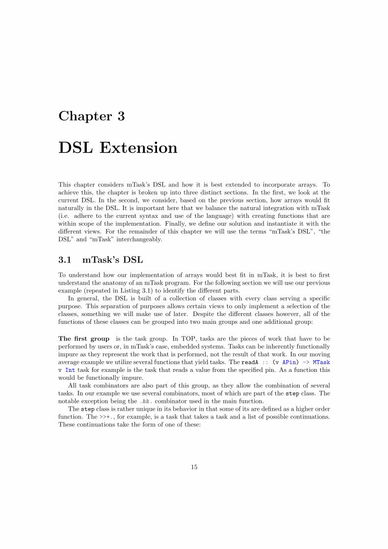
This chapter considers mTask’s DSL and how it is best extended to incorporate arrays. Toachieve this, the chapter is broken up into three distinct sections. In the first, we look at thecurrent DSL. In the second, we consider, based on the previous section, how arrays would fitnaturally in the DSL. It is important here that we balance the natural integration with mTask(i.e. adhere to the current syntax and use of the language) with creating functions that arewithin scope of the implementation. Finally, we define our solution and instantiate it with thedifferent views. For the remainder of this chapter we will use the terms “mTask’s DSL”, “theDSL” and “mTask” interchangeably.

3.1 mTask’s DSL

To understand how our implementation of arrays would best fit in mTask, it is best to firstunderstand the anatomy of an mTask program. For the following section we will use our previousexample (repeated in Listing 3.1) to identify the different parts.

In general, the DSL is built of a collection of classes with every class serving a specificpurpose. This separation of purposes allows certain views to only implement a selection of theclasses, something we will make use of later. Despite the different classes however, all of thefunctions of these classes can be grouped into two main groups and one additional group:

The first group is the task group. In TOP, tasks are the pieces of work that have to beperformed by users or, in mTask’s case, embedded systems. Tasks can be inherently functionallyimpure as they represent the work that is performed, not the result of that work. In our movingaverage example we utilize several functions that yield tasks. The readA :: (v APin) -> MTask

v Int task for example is the task that reads a value from the specified pin. As a function thiswould be functionally impure.

All task combinators are also part of this group, as they allow the combination of severaltasks. In our example we use several combinators, most of which are part of the step class. Thenotable exception being the .&&. combinator used in the main function.

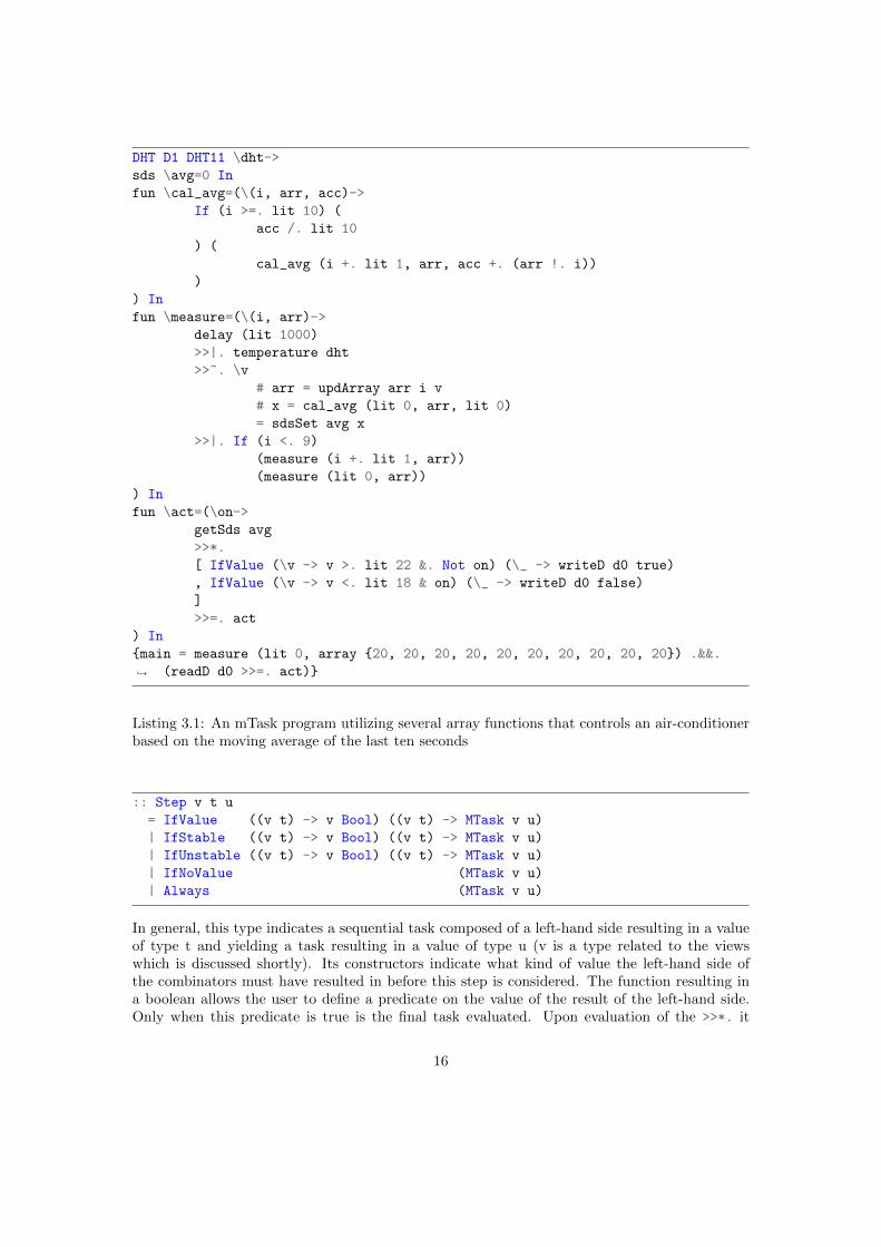
The step class is rather unique in its behavior in that some of its are defined as a higher orderfunction. The >>*., for example, is a task that takes a task and a list of possible continuations.These continuations take the form of one of these:

15

DHT D1 DHT11 \dht->

sds \avg=0 In


If (i >=. lit 10) (

acc /. lit 10

) (


)

) In


delay (lit 1000)


>>~. \v



= sdsSet avg x

>>|. If (i <. 9)



) In

fun \act=(\on->

getSds avg

>>*.



]

>>=. act

) In



Listing 3.1: An mTask program utilizing several array functions that controls an air-conditionerbased on the moving average of the last ten seconds

:: Step v t u

= IfValue ((v t) -> v Bool) ((v t) -> MTask v u)

| IfStable ((v t) -> v Bool) ((v t) -> MTask v u)

| IfUnstable ((v t) -> v Bool) ((v t) -> MTask v u)

| IfNoValue (MTask v u)

| Always (MTask v u)

In general, this type indicates a sequential task composed of a left-hand side resulting in a valueof type t and yielding a task resulting in a value of type u (v is a type related to the viewswhich is discussed shortly). Its constructors indicate what kind of value the left-hand side ofthe combinators must have resulted in before this step is considered. The function resulting ina boolean allows the user to define a predicate on the value of the result of the left-hand side.Only when this predicate is true is the final task evaluated. Upon evaluation of the >>*. it

16

selects the first member of the continuation list for which both the constructor and predicatematch and evaluates the associated task. Take the following snippet from our example programas illustration:

getSds avg

>>*.



]

Both continuations of this step combinator are only considered if the task on the left-hand sideproduced a value. For getSds this is always. The combinator will then go on and check thepredicates of each of the possible continuations. Suppose our room temperate over the past 10seconds was 17 degrees and that our air-conditioner is currently on. The step combinator willcheck the first predicate, determine it is false (as per our hypothetical situation) and subsequentlyassess the second predicate. It will determine that this predicate is indeed true, and will resultin the writeD d0 false task. This task will then go on to turn off the air-conditioning.

Besides the >>*. combinators, other functions of the class implement less general versionsusing one of these continuations. For example the >>=. task:

(>>=.) infixl 0 :: (MTask v t) ((v t) -> MTask v u) -> MTask v u

(>>=.) ma amb = ma >>*. [IfValue (\_->lit True) amb]

Every program (but not every function) created with mTask has to be a task. One of thesimplest tasks (and thus mTask programs) you could define would be:

{main = rtrn (lit 42)}

Where the rtrn task takes a value and turns it into a task resulting in the value.

The second group is the expression class and all its functions. Functions in this group arecompletely evaluated during the interpretation phase. In our example the entire implementationof the cal_avg function is part of this domain. The same is true for all other mathematicalexpressions in the example. In iTasks, this domain is inhabited by all native Clean expressions.Of course this is not possible for mTask whose expressions depend on values stored on theembedded device. Instead, mTask has a class specifically inhabiting this domain, the expr class.

The additional group is the group that lives outside of the main function, in our movingaverage example these would be the sds and fun functions. Classes in this category usuallyserve to create some construct whose scope is the entire program. Other classes with functionsin this domain are the peripheral classes, classes that interact with some sensor or actuator onthe embedded systems. Several functions that take some value that was created by a functionin this group are tasks. This has to do with the functional impurity of certain functions in thisgroup.

An excerpt of a selection of mTask’s classes relevant to our example is given in Listing 3.2.In them, v is a type constructor with kind * -> *, that expresses a view on the DSL. There arethree views implemented on mTask’s classes, two of which are evaluated using a monad, the last

17

class expr v where

lit :: t -> (v t)

(+.) infixl 6 :: (v t) (v t) -> (v t) | + t

(/.) infixl 6 :: (v t) (v t) -> (v t) | / t

If :: (v Bool) (v t) (v t) -> v t

class step v | expr v where

(>>*.) infixl 1 :: (MTask v t) [Step v t u] -> MTask v u

(>>=.) infixl 0 :: (MTask v t) ((v t) -> MTask v u) -> MTask v u

(>>|.) infixl 0 :: (MTask v t) (MTask v u) -> MTask v u

class (.&&.) infixr 4 v :: (MTask v a) (MTask v b) -> MTask v (a, b)

Listing 3.2: Excerpts of classes definitions relevant to our air-conditioner example

(TraceTask) lives inside iTasks and is evaluated as an iTask task. For our instances of the threeviews we will deviate from our normal example for a while, instead using the following exampleto dramatically decrease verbosity:

rtrn (lit 1) >>=. \i -> rtrn (i +. lit 1)

3.1.1 The Show View

Firstly, there is the show view whose purpose is to convert the mTask task into a humanreadable string. Listing 3.3 displays the show instance for the classes depicted in Listing 3.2.Where show and binop are implemented as such:

show :: String -> Show a

show s = Show \st -> (undef, st +++ s)

binop x o y = show "(" >>| x >>| show o >>| y >>| show ")"

and with a show type that keeps track of the current state. Holding, for example, the currentlevel of indentation and a list of identifiers.

:: Show a = Show (ShowState -> (a, ShowState))

It is worth noting that the show view in mTask does not produce a String. Rather, for efficiencyreasons1, it produces a [String].

Our small example program results in the following:

(rtrn 1) >>= \a0.(rtrn (a0+1))

1An String in Clean is represented as an array of Char. Constantly appending or prepending is very inefficient.This appending and prepending is avoided by using a lazy list of String.

18

instance expr Show where

lit t = show (toString t)

(+.) x y = binop x "+" y

(/.) x y = binop x "/" y

If c t e = show "If" >>| show " " >>| c >>| t >>| e

instance step Show

where

(>>*.) e l = e >>| show " >>*" >>| indent >>| nl

>>| show "[" >>| showSteps l >>| show "]" >>| unIndent >>| nl

(>>=.) e l = e >>| show " >>= " >>| indent >>| nl >>| fresh "a" >>=

\i->show ("\\" + i + ".") >>| f (show i) >>| unIndent

(>>|.) e l = e >>| show " >>| " >>| indent >>| nl >>| f >>| unIndent

instance .&&. Show where (.&&.) x y = x >>| nl >>| show ".&&." >>| nl >>| y >>|

return undef

Listing 3.3: The Show instance of the classes given in Listing 3.2

instance expr Interpret where

lit t = tell (BCPush (toByteCode t))

(+.) a b = a >>| b >>| tell (binop a BCAddI BCAddL BCAddR)

(-.) a b = a >>| b >>| tell (binop a BCSubI BCSubL BCSubR)

(/.) a b = a >>| b >>| tell (binop a BCDivI BCDivL BCDivR)

If c t e = freshlabel >>= \elselabel->freshlabel >>= \endiflabel->

c >>| tell (BCJumpF elselabel) >>|

t >>| tell` [BCJump endiflabel, BCLabel elselabel] >>|

e >>| tell (BCLabel endiflabel)

Listing 3.4: The Interpret instance of the expr class as defined in Listing 3.2

Note that the identifier of the lambda’s argument is lost during Clean’s compilation. As such, anew identifier (a0) was created by the view.

3.1.2 The Interpret View

In addition to the show view, mTask also contains a view to compile the mTask to bytecode.This bytecode is sent to the RTS where it is interpreted. The concept behind the interpret viewis that every function generates its own code, this code is then collected into a single program bythe monad. Additionally, the monad has functions that deal with other aspects of compilatione.g. a function exists that returns a new free identifier. Consider the subset of the expr classfrom before, but this time instantiated by the interpret view in Listing 3.4.

To fully understand this instance, we must take a small detour to the monad used here. Thismonad2 (which we will call the interpret monad for now), is very similar in behavior to the State

2In reality this monad is a StateT monad holding a Writer monad, but this detail can be overlooked. It is only

19

binop :: (v a) BCInstr BCInstr BCInstr -> BCInstr | type a

binop a i l r = if (byteWidth a == one) i

(if (isReal (cast1 a)) r l)

Listing 3.5: The binop function found in the mTask system

monad if the state were a tuple of two values. These values would be a record with type BCState

(holding data needed for compilation) and the final program represented as a [BCInstr]. Thetell function appends instructions to this second state.

Additionally, we must quickly describe how code is evaluated on the embedded devices ingeneral, a more detailed version is discussed in Chapter 5. For evaluation of mTask programsthere are two relevant memory sections: the stack and the heap. The stack is used primarilyduring the interpretation of the expressions of group two. The heap is used to store the tasknodes that form the task tree. In our example, for instance, the sdsSet function creates asdsSet-node on the heap. The value x that was created from an expression is, at this point,copied from the stack to the heap, being part of this sdsSet-node.

Given these explanations, we can now see that the lit function transforms a value to itsbyte representation and pairs that with an instruction that pushes these bytes to the stack.The addition does something a little more interesting, in that it first determines what type weare trying to add. Based on the type, it will then select the appropriate addition instruction.Listing 3.5 show this function. The byteWidth function is used to determine if the value is aninteger as integers are the only values occupying a single stack space. Reals and Longs bothoccupy two stack cells and such a different function is used here, the isReal function results intrue only if its argument has type :: Real. Finally, the cast1 function is a function with typesignature cast1 :: (v a) -> a required to access the type contained in v.

Consider first only rtrn (lit 1) and how it compiles before we see at how it integrateswith the task as a whole. First, 1 should be pushed onto the stack, this is performed using theBCPush instruction. Thereafter, the top of the stack should be used to create a task node, thisis achieved using the BCMkTask instruction, where the argument should be BCStable. In short,we end up with the following list of instructions to create a stable node holding the number 1.

0: BCPush 0 1 // Push 1 on the stack, the values 0 and 1 form

// the byte representation of the 16 bit integer

1.↪→

4: BCMkTask BCStable1 // Create a single stable node containing the

// value. The 1 is the value's stackwidth

This stable node is used as an argument for the step node, whose other argument is a pointerto the function on its right side. During interpretation, the step node will use the value on theleft side as an argument for the function(s) on its right side. To do this, it evaluates its left sidefully (pushing it on the stack), checks if the value matches the predicate (which is always truein our case), and then interprets the right-hand side. The right-hand side finally uses the valueon the stack as an argument.

In the end, the program will look as given in Listing 3.6, where all instructions are accompa-nied by a comment describing them.

important that the behavior of the tell function is introduced.

20

0: BCJump 15 // Jump to the main function

3: BCArg 0 // Take argument 0 and push it on the stack

5: BCPush 0 1 // Push 1 on the stack

9: BCAddI // Add the two integers on top of the stack

10: BCMkTask BCStable1 // Create a stable node containing

// the top of the stack

12: BCReturn 1 2 // Return the result from this function

15: BCPush 0 1 // Push 1 on the stack

19: BCMkTask BCStable1 // Create a stable node containing

// the top of the stack

21: BCMkTask BCStepStable 1 3 // Create the step task, with 1 denoting the

// stackwidth of the value and

// the function starting at 3 as the function

26: BCReturn 1 0 // Return top of the stack with width 1 knowing

// that this function had 0 arguments

Listing 3.6: The bytecode instructions compiled from rtrn (lit 1) >>=. \i -> rtrn (i +.

(lit 1)) accompanied by a summary of their semantics

3.1.3 The TraceTask View

Lastly, there exists the TraceTask view, an interpreter of the tasks written in Clean and incor-porated into the library. This view is itself integrated into iTask, in the uniqueness chapter wewill discuss this detail further. The result of the tracetask view on our small example is a stable2.

3.1.4 Interpretation

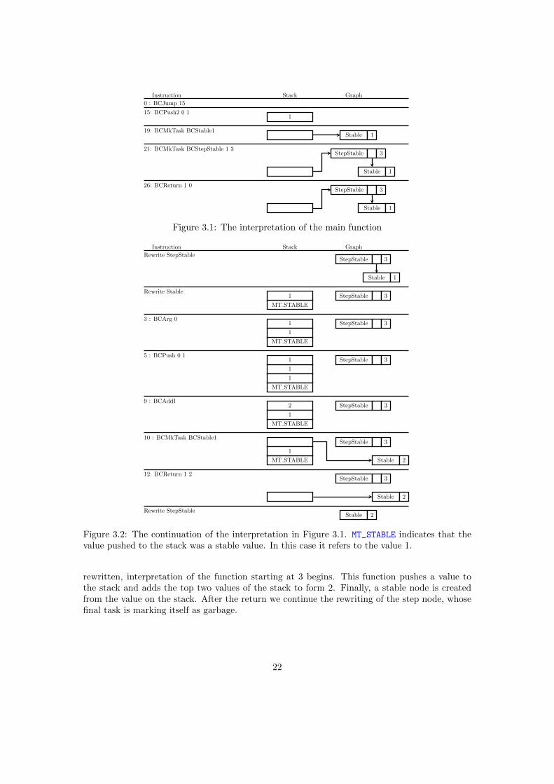
Once the bytecode is generated, it is interpreted in the RTS where it is used to build a tree, thistree is then rewritten in a later phase. We already saw that the main function of our exampleprogram creates a stable node containing the value 1, but let’s now consider the entire programand the tree it builds. Figure 3.1 shows the interpretation of the main function step by step.The stack and tree are shown as they would be after the interpretation of the instruction. Dueto the way the bytecode in mTask is laid out, the first instruction is a jump, this jump jumps tothe entry point of the main function. The second instruction pushes a value to the stack. In thethird instruction this value is used to create the first node of the tree, a stable node. This nodeholds the value that was earlier pushed to the stack. In addition to the creation of the stablenode, this instruction also pushes a reference to the newly created node to the stack. The next(fourth) instruction creates a step node. The two integer arguments of this instruction depictthe width of the argument and function reference respectively. The step node has two references,the first references the value of the lhs, this side has already been evaluated to be “Stable 1”.The “3” references the entry point of the function on the rhs of the step combinator. The finalinstruction moves the reference to the step node into the return space on the stack and dealswith the frame pointer and other bookkeeping.

After the completion of the main function, the rewriting of the graph will begin. Rewritingthe graph starts at the root node (the StepStable node in this case). The StepStable node isspecial in the sense that it will rewrite its left hand side, and then interpret the function onits right hand side. This behavior is depicted in Figure 3.2. Once the stable node has been

21

Stack GraphInstruction

0 : BCJump 15

15: BCPush2 0 11

19: BCMkTask BCStable1Stable 1

21: BCMkTask BCStepStable 1 3StepStable 3

Stable 1

26: BCReturn 1 0StepStable 3

Stable 1

Figure 3.1: The interpretation of the main function

Stack GraphInstruction

StepStable 3

Stable 1

Rewrite StableStepStable 3

MT STABLE

1

3 : BCArg 0StepStable 31

5 : BCPush 0 1StepStable 3

1

1

9 : BCAddIStepStable 32

10 : BCMkTask BCStable1StepStable 3

Stable 2

12: BCReturn 1 2StepStable 3

Stable 2

Rewrite StepStable

Stable 2Rewrite StepStable

MT STABLE

1

MT STABLE

1

MT STABLE

1

MT STABLE

1

Figure 3.2: The continuation of the interpretation in Figure 3.1. MT_STABLE indicates that thevalue pushed to the stack was a stable value. In this case it refers to the value 1.

rewritten, interpretation of the function starting at 3 begins. This function pushes a value tothe stack and adds the top two values of the stack to form 2. Finally, a stable node is createdfrom the value on the stack. After the return we continue the rewriting of the step node, whosefinal task is marking itself as garbage.

22

3.2 Expression versus Task

In the example program it is shown that we have chosen to implement arrays as being part ofexpressions. This can be seen in the way arrays are used directly in the expressions. Anotheroption would be creating the array with a function in the first group (outside the main function)and then having all operations on the array yield tasks. In reality, this was never a considerationbut it is important to see why. So in this section we consider why we found expressions to bebest suited to host arrays, and differences in implementation that would arise.

The strongest case for integrating arrays with expressions is a conceptual one. The arrayfunctions deal with pure values, they do not belong in the domain that hosts functionally impuretasks and their combinators.

Additionally, there is a distinct difference in the number of rewriting and interpretation phasesthat need to take place to achieve the same outcome. Suppose we have some function: (!.)

infixl 9 :: (v {a}) (v Int) -> v a we could then write:

rtrn (array {1,2,3} !. (lit 0) +. (lit 1))

This entire task requires a single interpretation and rewriting phase, where the only node rewrit-ten during the rewriting phase is the Stable node created by the rtrn function. The same is nottrue if we decide to implement the arrays as tasks, where the following would be equivalent:

(!.) infixl 9 :: (v {a}) (v Int) -> MTask v a

(array {1,2,3}) !. (lit 0) >>=. \x -> rtrn (x +. (lit 1))

Here, both the interpretation and the rewriting phase will happen twice. First, the array andselection are evaluated in the first interpret phase, resulting in the value 1. This value is thenused in the creation of the step node which is rewritten in the first rewriting phase. During thisrewriting, the step node will call for interpretation of its right-hand side (forming the secondinterpret phase). Finally, the result of this second interpret phase is used to create a stable nodewhich is ultimately rewritten during the final rewriting phase and sent back to the server.

The above is not to say that arrays in the task domain have no advantage. However, theonly advantages are that we (1) need not worry about functional purity and (2) could implementthe arrays as shares, making the implementation much easier because no effort would need to bemade in modifying the garbage collector. However, this would never allow the use of arrays inexpressions and would therefore make the RTS slower in most applications (having to constantlyswitch between interpretation and rewriting). Additionally, a lot of space would be used in thestorage of the array. Memory that might not be needed when having the array live in garbagecollectable memory. Most of all, this would never allow for arrays whose size is determined atruntime. Upon receival of a task all memory needed for the SDSs is allocated. As such, arraysimplemented as shares (in their current implementation) are required to specify their size uponcreation.

Concluding, while implementing arrays as tasks is much less complex, it would reduce theefficiency of the RTS and prevent arrays from changing in size as a consequence of the way theyare currently stored while having no other benefits. On the other hand, implementing them asexpressions takes more effort but results in a more satisfying and arguably better implementation.

23

3.3 The array class

Now that we have decided on a domain, a logical continuation is to decide on the functionsneeded to implement arrays and how we represent them in mTask. Obviously, we need some wayto create arrays. In our example program we saw the use of the array function, when it seemsthe lit function as described in the previous section should also suffice. This is because the lit

cannot be used in its current state, which has to do with the implementation of the function;a value passed to lit will be converted to its bytecode representation using the toByteCode

function which is then pushed on the stack in the RTS.


We will see later (in Chapter 5) that we want the arrays to live on the heap. Implying that the litfunction is not suited for arrays. For now, this means we can either change the implementationof the lit function, or create a separate array function. The difference being that the array

function allows all array related functions to be in a single class. Furthermore, in Chapter 4, wewill introduce uniqueness to the arrays, requiring a separation of functions either way3.

Given the above, the choice was made to create a separate array function.

array :: {a} -> v {a}

While it does not have the versatility of the lit function (not allowing simple creation of arraysin tuples for example), it does allow for a much cleaner implementation while not convolutingthe language by a significant amount. Similarly named functions can also be found in the likesof sds and the peripheral constructors. Additionally, we need some way to read data from thearray. We have already seen this function above in the examples.

select :: (v {a}) (v Int) -> v a

And some way to update the elements in the array4.

update :: (v {a}) (v Int) (v a) -> v {a}

The above functions are good in design, but functions with the same name as select andupdate already exist in an existing Clean module ( SystemArray). As such, we should renamethem to something else, i.e. to:

(!.) infixl 9 :: (v {a}) (v Int) -> v a

updArray :: (v {a}) (v Int) (v a) -> v {a}

The current expr class is given in Listing 3.7. We could extend this class to include the arrayfunctions described above, or we could decide to implement them as their own class:

3Not separating functions could potentially allow user of mTask to create non-unique arrays. Something wewish to avoid.

4Another option was a function of the type update :: (v a) (v Int) ((v a) -> v a) -> v {a} but higherorder functions are not supported in expressions by the current mTask ecosystem.

24

class expr v where

lit :: t -> v t

(+.) infixl 6 :: (v t) (v t) -> v t | + t

(-.) infixl 6 :: (v t) (v t) -> v t | - t

(*.) infixl 7 :: (v t) (v t) -> v t | * t

(/.) infixl 7 :: (v t) (v t) -> v t | / t

(&.) infixr 3 :: (v Bool) (v Bool) -> v Bool

(|.) infixr 2 :: (v Bool) (v Bool) -> v Bool

Not :: (v Bool) -> v Bool

(==.) infix 4 :: (v a) (v a) -> v Bool | Eq a

(!=.) infix 4 :: (v a) (v a) -> v Bool | Eq a

(<.) infix 4 :: (v a) (v a) -> v Bool | Ord a

(>.) infix 4 :: (v a) (v a) -> v Bool | Ord a

(<=.) infix 4 :: (v a) (v a) -> v Bool | Ord a

(>=.) infix 4 :: (v a) (v a) -> v Bool | Ord a

If :: (v Bool) (v t) (v t) -> v t

Listing 3.7: The expr class as defined for mTask

instance array BCInterpret

where

array arr = tell

[ BCPush (toByteCode arr)

, BCArrCreate (elemWidth arr) (size arr)

]

(!.) arr i = arr >>| i >>| tell [BCArrSelect]

updArray arr i a = a >>| arr >>| i >>| tell [BCArrUpdate]

Listing 3.8: The Interpret instance of the array class

class array v where

array :: {a} -> v {a} | type a

(!.) infixl 9 :: (v {a}) (v Int) -> v a | type a

updArray :: (v {a}) (v Int) (v a) -> v {a} | type a

Arguably, the array functions do not fit in the expr class, where nearly all functions are designedto work on any basic type. Additionally, a separate class allows the views to chose not toimplement the arrays5. As such, we will use the second option of implementing their own class.

3.3.1 The Interpret View

All operations on arrays can not rely on current instructions since mTask does not currentlyproduce any bytecode that deals with memory management. Unfortunately, this leaves us with

5In Chapter 4 we will run into a situation where we do indeed discover that one of the views no longer supportsarrays.

25

instance array Show

where

array arr = show "array " >>| show (toString arr)

(!.) arr i = arr >>| show "!." >>| i >>| pure undef

updArray arr i a = show "updArray" >>| arr >>| i >>| a >>| pure undef

Listing 3.9: The Show instance of the array class

not much of a choice regarding compilation to bytecode. Every function should simply be com-piled to a new instruction as depicted in Listing 3.8. This listing also shows how similar the lit

and array functions are, with the array function simply appending an additional function thatreads the previously pushed data from the stack and creates an array node. Of course, anotheroption was to make use of the lit function:

array arr = lit arr >>| tell (BCArrCreate (elemWidth arr) (size arr))

But being reliant on a function of another class adds a dependency to the class and the imple-mentation.

3.3.2 The Show View

The show instance of the array class as shown in Listing 3.9 is relatively trivial. Simply replacingall the functions with a textual representation.

3.3.3 The TraceTask View

In Chapter 4 we will discover that this class cannot be implemented to the degree we want itto. This has to do with the fact that this view is an iTask, and that iTasks cannot operate on(optionally) unique values. As such, there exists no implementation for this view of the array

class. Due to the nature of mTask’s class based structure this does not pose a problem, as long aswe do not attempt to trace a task containing one or more functions from the array class. Shouldwe attempt to do so, the Clean compiler will throw an error and fail to compile our program.

26

Chapter 4

Uniqueness

Clean is a functionally pure programming language, i.e. every function is guaranteed to:

1. Produce the same output given the same arguments

2. Produce no side effects

While this has many advantages, two major disadvantages of its implementation are the spacebehavior problem and the usage of inherently impure computations. The space behavior prob-lem references the fact that values cannot be updated destructively. Consider for example thefollowing program:

f :: {Int} -> ({Int}, Int)

f a = (update a 0 2, select a 0)

Start = f {1,2,3}

Let it be known that select is given {1,2,3} and 0 as arguments through Start. If we assumeupdate updates the array destructively, the result of this program is ({2,2,3}, 2). However,when we change the Start to Start = snd (f {1,2,3}), update is omitted due to lazy evalua-tion and the result is 1, violating requirement one of functional purity. To solve this, functionallypure languages copy every value that is changed. For the update function, a copy of the fullarray is made where the first element is replaced with a 2. The original array is still passed tothe select resulting in the value ({2,2,3}, 1).

This is obviously not ideal for embedded systems that (in general) do not have much memory.For mTask the decision was made that arrays should only be implemented if it were possible todo this in a destructive manner to avoid this memory issue. A possible solution, in the formof uniqueness typing, is presented in this chapter. As a quick introduction, uniqueness typingenforces that only a single reference may exists to a value at any one time. This allows mutableupdates to take place without producing side effects. Of course this comes with disadvantages,code written without uniqueness in mind does not always have an equivalent unique alternative.Additionally, writing code with uniqueness in mind is not a trivial endeavour and comes with itsown set of challenges.

Uniqueness is first introduced after which, in the second section, we attempt to write themTask ecosystem in such a way that it is able to support uniqueness typing, thus enablingfunctionally pure mutable arrays.

27

dup

x

(a) The graph when x is passed to dup but thefunction has not yet been evaluated.

(,)

x

(b) After the evaluation of dup, the tuple nodeshows that multiple references to a single valuecan exist.

Figure 4.1: The evaluation of a simple dup function duplicating some non-unique value.

4.1 Uniqueness

Uniqueness typing is a type system introduced by Barendsen and Smetsers [2] in an effort tosolve the space behaviour problem and the problem regarding functionally impure operationsin a graph rewriting setting. A value is said to be unique if it is guaranteed there exists atmost one reference to it. This single reference guarantee allows the programmer to write codethat destructively updates said value without modifying the semantics of the program (the spacebehavior problem). Additionally, it allows for functionally impure computations such as I/O. FileI/O, for example, is handled in Clean using unique file handles, preventing any non-sequentialwrites to a file. For mTask’s arrays, we are mostly interested in the solution to the space behaviorproblem, but a global understanding is still desirable.

To achieve this single reference property, the system extends conventional Milner/Mycrofttyping with uniqueness annotations. In Clean, a type can be annotated using one of threeannotations, giving four options in total:

a

*a

.a

u:a (where u is any identifier)

Normally Clean places no restrictions on the way a value is used. It is perfectly fine to createtwo references to a single value in the graph. In fact this is one of the strengths of graph rewritingover naive term rewriting because it avoids copying a value needlessly. In the following examplefor instance, we create a tuple holding the same value twice:

dup :: a -> (a, a)

dup x = (x, x)

Internally, the result of dup would be represented as a node with two references to the samevalue. Figure 4.1 shows exactly this concept by applying dup to some value x.

Annotating a type with ”*” enforces that there exists at most one reference to the value. Forinstance, we cannot implement our dup function in the same way as above if we want to changethe type to accept a unique argument:

dupu :: *a -> (*a, *a)

This is due to the fact that the dup function creates two references to our unique value, violatingthe single reference constraint. In fact, it is impossible to create a total function with this type.

The above mentioned problem also holds when using the following type for dup:

28

dupo :: .a -> (.a, .a)

Here, a is a value that is optionally unique (i.e. both non-unique and unique values should beaccepted by this function). This means that the implementation must be valid regardless ofwhether the value of type a is unique, which might not be the case. The following programdemonstrates this fact:

Start = dupo i

where

i :: Int

i = 42

As with our dupu function, no implementation of this function exists.Finally, uniqueness variables can be used to enforce the same attribute on multiple types,

or in coercion statements to enforce relations on the uniqueness attributes, which allow theprogrammer to place restrictions on the uniqueness attributes of types in relation to each other.The uniqueness inequality u <= v enforces that u is unique if v is unique. This is often used insituations where one value is wrapped in another. For example, a tuple containing one or moreunique values should be unique itself as expressed in the following type.

tuple :: v:a w:b -> u:(v:a, w:b), [u <= v, u <= w]

Given that a function is guaranteed to have a unique reference to a unique value, the compilercan compile this function in such a way that it destructively updates the unique value. This iswhat we meant earlier when we talked about the space behaviour problem and is incrediblypowerful in the sense that it can prevent the constant copying of large nodes. It is for thisreason the Clean standard library (StdEnv) makes heavy use of uniqueness in its Array module(_SystemArray) where many functions come in pairs of two, with one accepting non-uniquearrays and the other accepting the unique counterpart. Consider the size :: {e} -> Int

function for example, if the size function would naively accept unique arrays, the array wouldbe consumed, and it would no longer be possible to pass the array to another function as well.Instead, a unique version of the function should also return the unique array such that it can beused elsewhere. Their difference is reflected in their types:

size :: {e} -> Int

usize :: u:{e} -> *(Int, u:{e})

This construct, where the unique counterpart of a function returns a tuple with the intendedresult and the unique argument can be found in many places dealing with uniqueness, anotherexample being the StdFile library.

4.2 The Unique Array Class

Now that we have introduced uniqueness and have shown that it can be used to create mutablevalues, we should change our array class to produce unique arrays. This way, interpretation canhappen in a destructive manner while preserving functional purity. We eluded to the fact that

29

functions for unique arrays have a different signature than functions for non-unique arrays, inthat unique values should be part of the result of a function such that they can be used again.In our previously defined array class, we should take these differences into account. Recall theclass defined earlier, but extended with the uniqueness annotations we want the class to have.

class array v where

array :: *{a} -> *(v *{a}) | type a

(!.) infixl 9 :: *(v *{a}) (v Int) -> v a | type a

updArray :: *(v *{a}) (v Int) (v a) -> *v *{a} | type a

Here, the (!.) function consumes the array, something we wish to avoid. In order to fix this,the function type should be modified such that it returns not only the value we wish to selectfrom the array, but also the array itself:

class array v where

array :: *{a} -> *(v *{a}) | type a

(!.) infixl 9 :: *(v *{a}) (v Int) -> *v (a, *{a}) | type a

updArray :: *(v *{a}) (v Int) (v a) -> *v *{a} | type a

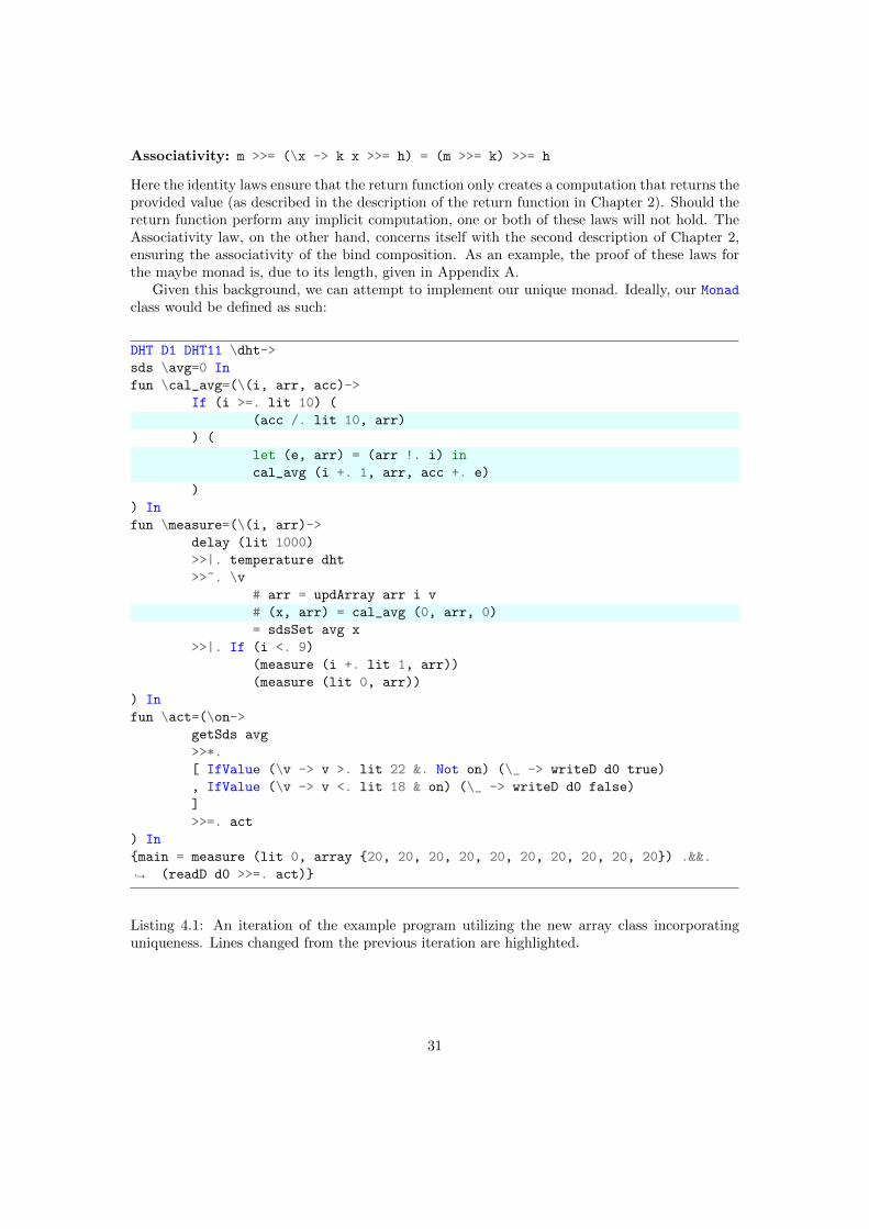
Of course, this change should also be reflected in our example program. We will have to constantlypass the array as to not lose our single reference to it. Listing 4.1 show the updated version ofour earlier example using the new array class and demonstrating the fact that the array must bepassed from one function to another.

Now that we have modified our example program, we should ensure that the entire ecosystemhas support for our unique arrays. The remainder of this chapter attempts this.

4.3 The Unique Monad

We have seen earlier that the mTask DSL (and TOP in general) has many similarities to aMonad. Additionally, we have seen that Monads are widely used in the compilation and printingof mTask. Now that the DSL produces optionally unique values, mTask’s backend must be ableto handle them. This leaves us with two possibilities; we either create a monad class that canresult in optionally unique values, or we rewrite every backend of mTask to no longer make useof any monad. The second option is not viable and would result in code that is very convoluted.As such, this section is dedicated to creating a new definition of the monad class that can beused in mTasks backend to allow unique arrays.

Before we dive into the implementation of our uniqueness monad, we should quickly discussthe work by Jennifer Paykin and Steven Zdancewic on their linearity monad [18]. A criticaldifference in the monad they implemented and the monad we will implement below is that ourmonad does not deal with a linear state, rather, it is supposed to be able to result in uniquevalues (the unique arrays). Additionally, it is important to introduce a set of constraints. Anyinstantion of the monad class as defined in Chapter 2 should (but is not forced to) abide to the socalled monad laws, ensuring that the implemented functions abide to their descriptions. Thesemonad laws are as follows. For every a, h, k, m it holds that:

Left Identity: return a >>= k = k a

Right Identity: m >>= return = m

30

Associativity: m >>= (\x -> k x >>= h) = (m >>= k) >>= h

Here the identity laws ensure that the return function only creates a computation that returns theprovided value (as described in the description of the return function in Chapter 2). Should thereturn function perform any implicit computation, one or both of these laws will not hold. TheAssociativity law, on the other hand, concerns itself with the second description of Chapter 2,ensuring the associativity of the bind composition. As an example, the proof of these laws forthe maybe monad is, due to its length, given in Appendix A.

Given this background, we can attempt to implement our unique monad. Ideally, our Monadclass would be defined as such:

DHT D1 DHT11 \dht->

sds \avg=0 In


If (i >=. lit 10) (

(acc /. lit 10, arr)

) (

let (e, arr) = (arr !. i) in

cal_avg (i +. 1, arr, acc +. e)

)

) In


delay (lit 1000)


>>~. \v


# (x, arr) = cal_avg (0, arr, 0)

= sdsSet avg x

>>|. If (i <. 9)



) In

fun \act=(\on->

getSds avg

>>*.



]

>>=. act

) In



Listing 4.1: An iteration of the example program utilizing the new array class incorporatinguniqueness. Lines changed from the previous iteration are highlighted.

31

class Monad m | Applicative m

where

bind :: u:(m .b) .(.b -> v:(m .c)) -> v:(m .c)

Unfortunately, this is not allowed. Every type variable in a function type must have the sameuniqueness attribute. A possible solution would be to implement the bind outside the Monadclass or extend the Monad class to take three arguments1:

class Monad m n o | Applicative m

& Applicative n

& Applicative o

where

bind :: u:(m .b) .(.b -> v:(n .c)) -> v:(o .c)

This is not ideal, but something we might consider nonetheless. The previously mentioned showinstance could have the accompanying bind type or class instance:

bind :: u:(ShowM .b) .(.b -> v:(ShowM .c)) -> v:(ShowM .c)

instance Monad ShowM ShowM ShowM

With:

:: ShowM a = ShowM .(ShowState -> .(a, ShowState))

For now, we will only consider the bind function separately from the Monad class. Of course itcould still be placed back into the class if necessary.

The issue with the aforementioned type signature becomes apparent when trying to createan accompanying implementation. Let’s try to derive the uniqueness constraints of the followingfunction where all uniqueness attributes are variables for clarity.

bind :: u:(ShowM v:a) w:(v:a -> x:(ShowM y:b)) -> x:(ShowM y:b)

bind (ShowM a) f = ShowM (\s

# (v, s`) = a s

# (ShowM a`) = f v

= a` s`)

Given that the u in u:(ShowM v:a) propagates as such:

:: u:ShowM v:a = u:ShowM u:(ShowState -> u:(v:a, ShowState))

We get

1Note that these two solutions are essentially the same. The return statement needs to be lifted out of Monadclass any way, or a choice needs to made as to which class argument the return should operate on.

32

[u <= v, x <= y]

We also know that the u is propagated to (v, s`), whose type is u:(v:a, ShowState). Sincethis tuple with uniqueness annotation u is used the construction of the final value, we have [x

<= u]. This fact can also be demonstrated with the following function:

f :: u:a -> x:(b -> b), [x <= u]

f a = \s

# _ = a

= s

Where, though the result of a is not used, it is part of the ultimate construction, coercing theuniqueness of the result. This same reasoning can be applied to [x <= w], giving us our finallist of inequalities:

bind :: u:(ShowM v:a) w:(v:a -> x:(ShowM y:b)) -> x:(ShowM y:b)

, [u <= v, x <= y, x <= u, x <= w]

Consequently, as soon as we have one unique value in our monad, every subsequent m mustalso be unique. Essentially, this means that every function operating in the context of this monadinstance has to assume the encapsulating data type is unique. This is not a problem, but doesmean that the above type has no distinct advantage over the less generic type:

class Monad m where

bind :: *(m .a) (.a -> *(m .b)) -> *(m .b)

return :: .a -> *(m .a)

Since there is no advantage of the more generic type, this type was chosen instead. With thischange of the monad, all auxiliary functions and the DSL classes must also be modified to supportthe new unique type. All modifications to the auxiliary functions happened without much effort,and we will thus not discuss them in this thesis. The new classes were forced to have a uniquev in every function. The array, for example, was modified to be:

class array v where

array :: *{a} -> *(v *{a}) | type a

(!.) infixl 9 :: *(v *{a}) *(v Int) -> *v (a, *{a}) | type a

updArray :: *(v *{a}) *(v Int) *(v a) -> *v *{a} | type a

Finally, after creating this new monad class definition, we should consider its relation tothe monad laws described in the preliminaries. As a recap, there are three laws that a monadmust abide by in order to satisfy two desired properties: the left identity, the right identityand the associativity laws. Now, of course these laws are only relevant when considering someinstantiation of the class, but the class itself should at least not reject these laws by default, i.e.these laws should still be typeable in given the new class. Once typeable, we need not provethe laws for the unique instances because we have not changed their semantics. Looking at themonad laws (repeated below), the only possible problem is the reuse of identifiers on the left andright side of the equals sign. However, the sign denotes mathematical equality, outside the scopeof uniqueness, and thus poses no problem.

33

1. return a >>= k = k a

2. m >>= return = m

3. m >>= (\x -> k x >>= h) = (m >>= k) >>= h

As stated above, and assuming that the state monad abides by the monad laws2, this meansthat the modifications made to the monad class do not result in monad instances that do notabide by the monad laws.

4.4 The Unique Interpret View

Now that we have a monad class that can handle uniqueness, we can begin rewriting the backendto make use of this monad in order to support unique values. This in turn allows unique arrayswhich then grants us functionally pure mutability. In the interpret view, most interpret instanceswere trivially rewritten to deal with uniqueness, with a few notable exceptions.

Firstly, many classes use a value twice, once to push it to the stack, and a second time toinspect the stack width of the value. Inspecting the stack width happens using the toByteWidth3

class. Luckily, this class does not actually evaluate its argument:

instance toByteWidth Bool where toByteWidth _ = 1

instance toByteWidth Int where toByteWidth _ = 1

instance toByteWidth Long where toByteWidth _ = 2

instance toByteWidth Char where toByteWidth _ = 1

instance toByteWidth Real where toByteWidth _ = 2

...

The same is true for the expr class shown in Chapter 3, whose interpret instance is givenin Listing 3.4. In the instance, the binop function only uses the value a to determine whichaddition instruction should be used. For both these instances we have implemented a function:

duplicate :: .a -> .(.a, .a)

duplicate x = (undef, x)

Where undef is a value that aborts the program when evaluated with type: undef :: .a.However, since the undef value is only passed to functions where it is not evaluated, this is safe.Listing 4.2 show the interpret instance of the expr class (without the If function) using thisduplicate function. As modified version of the binop function is also given in the same listing.

Secondly, Clean’s if construct is defined as part of the language’s core with the type beingsomething along the lines of: if :: .Bool .a .a -> .a. This is in itself not a problem, butdoes allow the function to behave in ways undefinable in Clean itself4. Listing 4.4 shows twofunctions that both return 42. The second program, however, does not type check.

2In [11] it is shown that Haskell’s implementation of the state monad does actually not abide by the monadlaws.

3Despite what the name suggests, this function does not return the width of the value in bytes. Instead itreturns the width in terms of the number of stack cells a value of the type occupies.

4Technically, the if construct is part of Clean, what is meant here is a version of Clean that does not have theif construct.

34

instance expr Interpret where


(+.) a b

# (at, a) = duplicate a

= a >>| b >>| tell [binop at BCAddI BCAddL BCAddR]

(-.) a b


= a >>| b >>| tell [binop at BCSubI BCSubL BCSubR]

(/.) a b


= a >>| b >>| tell [binop at BCDivI BCDivL BCDivR]

binop :: .(v .a) BCInstr BCInstr BCInstr -> BCInstr | type, isReal a

binop v i l r

# (a, v) = cast1 v

= if (byteWidth v == one) i

(if (isReal a) r l)

Listing 4.2: The instance of the expr class using the duplicate function

f :: Bool *Int -> *Int

f b i = if b i i

Start = f True uniqueInt

where

uniqueInt :: *Int

uniqueInt = 42

Figure 4.2: Clean’s if construct allows tworeferences to a single unique value


f b i = my_if b i i

where

my_if :: Bool .a .a -> .a

my_if b t e = if b t e

Start = f True uniqueInt

where

uniqueInt :: *Int

uniqueInt = 42

Figure 4.3: Replication the duplication thatis possible with the if

Figure 4.4: Clean’s if construct allows the creation of multiple references to a unique value asshown in the first listing. Replicating this behavior using a function defined in Clean (as shownin the second listing) is not possible.

Appendix B shows other implementations of this function, none of which pass the uniquenesstype checking. When considering the definition of unique values, one might think that the firstprogram should not type check either. After all, creating two references to a single value isnot allowed. However, the if construct needs not create two references, since it can guaranteethat only one of the two unique values is evaluated. Currently, Clean’s compiler is not powerfulenough to identify that the second implementation does indeed also only ever evaluate one of thetwo values. This becomes an issue when implementing the step combinator for unique values.Recall that the step combinator takes a list of possible continuations as an argument, based on

35

predicates the suitable continuation is then selected. For this selection, mTask uses the internalIf function that is part of the expr class. By implementing uniqueness the type of the If

function was modified to: :: *(v Bool) *(v .a) *(v .a) -> *(v .a). Thus resulting in ourproblem. Using mTask’s If does not allow for continuation if any of the branches use the same(optionally) unique value. The only solution we found was lifting the implementation of the If

function directly into the implementation of the step combinator (i.e. the code used to createthe if function was used directly in the step combinator). Code copying was avoided using aClean macro (where the compiler will perform the code duplication before type checking takesplace). Recall our example program where we use an if statement to determine the argumentfor the recursive call of measure. Here, this exact problem also takes place. As a workaround,the if was only used to determine the value of i, as given in the version in Listing 4.3. Alsotake note of the nunique function used in the continuations of the step in our example program.The step function should be able to apply predicates on unique values. Of course, this meansthe predicate itself should also return the value. For those situations where we do not want topass our argument back, we can use this nunique f :== \p -> (f p, p) macro to wrap thefunction with.

Finally, Clean’s compiler does not allow uniqueness annotating in class constraints. Thefollowing program, for example, does not typecheck:

class f a b :: a -> b

g :: *(*v a, *v a) -> Int | f (*v a, *v a) Int

g x = f x

Instead showing an error that annotating v in the class constraint of g is not allowed. Generallythis is not a problem, since uniqueness attributes in the classes themselves can often be usedto express unique types. When uniqueness attributes are added to nested data types (as seenabove), however, this can no longer be done. The problem is best described using mTask’s fun

class which allows the definition of functions and is defined as such:

class fun a v :: ((a -> v s) -> In (a -> v s) (Main (MTask v u)))

-> Main (MTask v u)

Which was modified as follows to support unique values:

class fun a v :: ((*a -> *(v .s)) -> In (*a -> *(v .s)) (Main (MTask *v .u)))

-> Main (MTask *v .u)

Where MTask is a type synonym for v (.TaskValue a). In the mtaskfuns (a class that mustbe implemented by the views to allow the use of functions) class every possible arrangement ofarguments is a separate constraint:

36

DHT D1 DHT11 \dht->

sds \avg=0 In


If (i >=. lit 10) (


) (



)

) In


delay (lit 1000)


>>~. \v



= sdsSet avg x

>>=. \_

# i = If (i <. 9) (i +. lit 1) (lit 0)

= measure (i, arr)

) In

fun \act=(\on->

getSds avg

>>*.

[ IfValue (nunique (\v -> v >. lit 22 &. Not on)) (\_ -> writeD d0

true)↪→

, IfValue (nunique (\v -> v <. lit 18 & on)) (\_ -> writeD d0 false)

]

>>=. act

) In



Listing 4.3: A second iteration of example program utilizing uniqueness. In this version the If

function is used differently to avoid creating two references to the same unique array. Addition-ally, the nunique is introduced. Differences with the previous iteration are highlighted.

37

class mtaskfuns v

| fun () v

& fun (v DPin) v

...

& fun (v Real) v

& fun (v DPin, v DPin) v

& fun (v DPin, v Bool) v

...

& fun (v Real, v Real) v

& fun (v DPin, v DPin, v DPin) v

& fun (v DPin, v DPin, v Bool) v

...

& fun (v Real, v Real, v Real) v

When incorporating uniqueness, we would ideally have every v in the class constraints be aunique view, but, as written above, these are ignored by the compiler. Of course, the uniquenessattribute as defined in the fun class, do propagate to functions with an arity of one since theseare not nested types.

It is best to look at an example. Consider the fun (v Real) v and fun (v Real, v Real)

v instantiations. The first results in a fun function with the following type:

fun :: ((*(v Real) -> *(v .s)) -> In (*(v Real) -> *(v .s)) (Main (MTask *v

.u)))↪→


Where it is indeed true that every v is unique. However, when instantiating the second type, weend up with this:

fun :: ((*(v Real, v Real) -> *(v .s)) -> In (*(v Real, v Real) -> *(v .s))

(Main (MTask *v .u))) -> Main (MTask *v .u)

In which not every v is unique. Right now, this means that the mtaskfuns class has only thefollowing constraints:

class mtaskfuns v

| fun () v

& fun (v DPin) v

& fun (v Bool) v

& fun (v Int) v

& fun (v Long) v

& fun (v Real) v

Disallowing any function with an arity higher than one. A possible solution is to split the funclass into three separate classes, all describing a function with a different arity. These classescould possibly look like this:

38

class fun1 a v :: ((*a -> *(v .s)) -> In (*a -> *(v .s)) (Main (MTask *v .u)))


class fun2 a b v :: (((*a, *b) -> *(v .s)) -> In ((*a, *b) -> *(v .s)) (Main

(MTask *v .u))) -> Main (MTask *v .u)

class fun3 a b c v :: (((*a, *b, *c) -> *(v .s)) -> In ((*a, *b, *c) -> *(v

.s))↪→

(Main (MTask *v .u))) -> Main (MTask *v .u)

Attentive readers might realize that these classes still do not allow unique arrays as arguments.This can be achieved by further modifying the classes such that they either: only accept (op-tionally) unique values or have separate classes for arrays. Both solutions are not ideal, the firstbecause we really do not want basic values to ever have to be unique and the second because itadds even more classes. For the sake of completeness, separating the classes even further wouldresult in the following list:

class fun1 a v

class fun1a a v

class fun2 a b v

class fun2a1 a b v

class fun2a2 a b v

class fun2a12 a b v

class fun3 a b c v

class fun3a1 a b c v







In turn resulting the updated version of our example program as shown in Listing 4.4. While thecurrent mtaskfuns is already far from ideal, it should be clear that this approach is even worseand further changes are needed before even considering allowing arrays to be used as argumentsfor mTask functions. Ultimately, this means that arrays cannot currently be implemented in agood enough way for them to make a useful addition to mTask.

4.5 The Unique Show and TraceTask View

The show view often does not deal with duplicate values, and such was translated to a uniqueversion without much effort. The tracetask view, however, is, as mentioned in the Chapter 3, aniTask. Unfortunately, iTasks does not currently support the use of unique (or optionally unique)values. In the future, it would ideally be extended to have support for unique values (if possible),but until that time the tracetask view cannot be implemented for out unique version of mTask.

39

DHT D1 DHT11 \dht->

sds \avg=0 In

fun3a2 \cal_avg=(\(i, arr, acc)->

If (i >=. lit 10) (


) (



)

) In

fun2a2 \measure=(\(i, arr)->

delay (lit 1000)


>>~. \v



= sdsSet avg x

>>=. \_

# i = If (i <. 9) (i +. lit 1) (lit 0)

= measure (i, arr)

) In

fun1 \act=(\on->

getSds avg

>>*.


true)↪→


]

>>=. act

) In



Listing 4.4: A third iteration of example program utilizing uniqueness. In this version we nolonger use the fun function, instead using a selection of different function to avoid a typingproblem with classes and uniqueness. Differences with the previous iteration are highlighted.

40

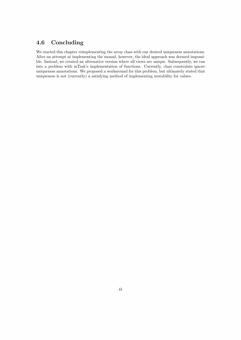
4.6 Concluding

We started this chapter reimplementing the array class with our desired uniqueness annotations.After an attempt at implementing the monad, however, the ideal approach was deemed impossi-ble. Instead, we created an alternative version where all views are unique. Subsequently, we raninto a problem with mTask’s implementation of functions. Currently, class constraints ignoreuniqueness annotations. We proposed a workaround for this problem, but ultimately stated thatuniqueness is not (currently) a satisfying method of implementing mutability for values.

41

Chapter 5

Runtime System

In the beginning of this thesis, we mentioned that the current RTS was not made having mutablecollection types in mind. In particular, it has no support for any kind of nodes larger than atypical combinator node. If we want to implement arrays in mTask, we will have to change this,requiring changes to many parts of mTask’s RTS. In this chapter of the thesis we first introducethe current RTS to get familiar with the parts that need changing. Given this basis, we will thenmodify the RTS to support arrays.

5.1 The RTS

To understand what parts of the RTS do not support what is needed for arrays, it is best tofirst take a global look at its implementation, highlighting everything that must be modified. Allinformation in this section describes the runtime system as it was before any changes were madetowards implementing arrays.

5.1.1 Memory Layout

Earlier we saw that, during interpretation, the mTask RTS needs at least a stack (to storeexpression values on and to return the pointer to the root node) and a heap (to store the nodesthat make up the task tree). In addition to those sections of memory, mTask also contains atask heap that is used to store information about the tasks received from the server, includingbut not limited to: an identifier, bytecode, a pointer to the root node and a section reserved forthe return value. mTask’s memory layout is depicted in Figure 5.1 each section of which will bediscussed below.

The Heap

The heap in mTask’s RTS stores the tree of all tasks currently being worked on by the RTS.Nodes in this section of memory are managed by the garbage collector, which we will discusslater. The tree consists of a collection of nodes, with every node having zero or more referencesto children and no two nodes having references to the same node (this property allows mTasknot to have a dedicated garbage marking phase). Figure 5.2a shows the general layout of a singlenode where the data is dependent on whichever type the node has. The task_type of the noderepresents the kind of data this node stores and is used during rewriting to determine in whatway the node should be rewritten. trash is a flag that indicates if the node should be garbage

42

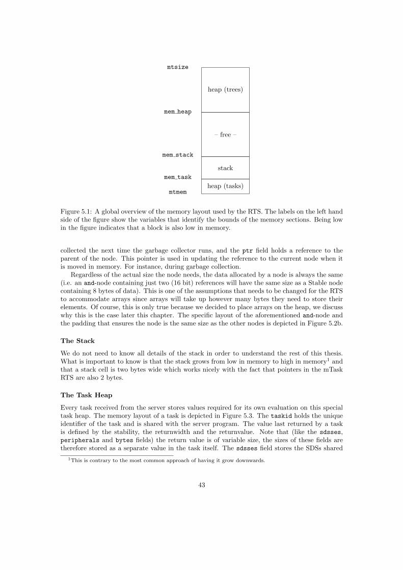
mtsize

mem heap

heap (trees)

mem stack

– free –

mem task

stack

mtmemheap (tasks)

Figure 5.1: A global overview of the memory layout used by the RTS. The labels on the left handside of the figure show the variables that identify the bounds of the memory sections. Being lowin the figure indicates that a block is also low in memory.

collected the next time the garbage collector runs, and the ptr field holds a reference to theparent of the node. This pointer is used in updating the reference to the current node when itis moved in memory. For instance, during garbage collection.

Regardless of the actual size the node needs, the data allocated by a node is always the same(i.e. an and-node containing just two (16 bit) references will have the same size as a Stable nodecontaining 8 bytes of data). This is one of the assumptions that needs to be changed for the RTSto accommodate arrays since arrays will take up however many bytes they need to store theirelements. Of course, this is only true because we decided to place arrays on the heap, we discusswhy this is the case later this chapter. The specific layout of the aforementioned and-node andthe padding that ensures the node is the same size as the other nodes is depicted in Figure 5.2b.

The Stack

We do not need to know all details of the stack in order to understand the rest of this thesis.What is important to know is that the stack grows from low in memory to high in memory1 andthat a stack cell is two bytes wide which works nicely with the fact that pointers in the mTaskRTS are also 2 bytes.

The Task Heap

Every task received from the server stores values required for its own evaluation on this specialtask heap. The memory layout of a task is depicted in Figure 5.3. The taskid holds the uniqueidentifier of the task and is shared with the server program. The value last returned by a taskis defined by the stability, the returnwidth and the returnvalue. Note that (like the sdsses,peripherals and bytes fields) the return value is of variable size, the sizes of these fields aretherefore stored as a separate value in the task itself. The sdsses field stores the SDSs shared

1This is contrary to the most common approach of having it grow downwards.

43

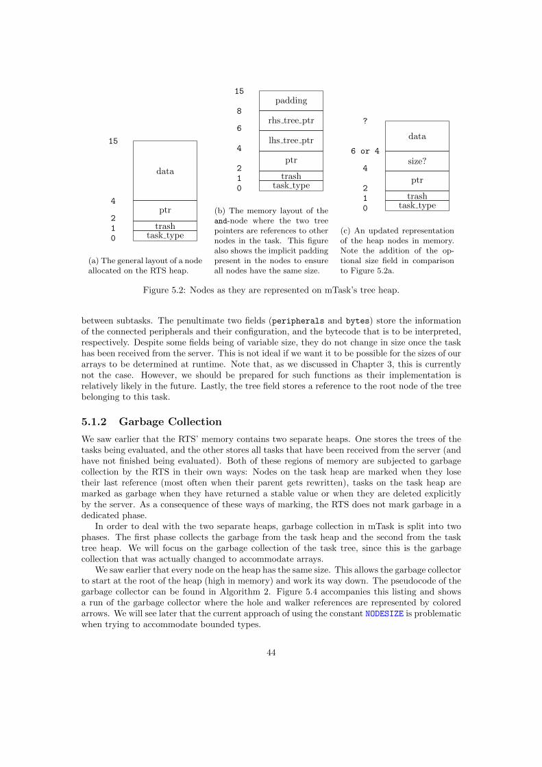
15

4

data

2ptr

1 trash

0 task type

(a) The general layout of a nodeallocated on the RTS heap.

15

8padding

6rhs tree ptr

4lhs tree ptr

2ptr

1 trash

0 task type

(b) The memory layout of theand-node where the two treepointers are references to othernodes in the task. This figurealso shows the implicit paddingpresent in the nodes to ensureall nodes have the same size.

?

6 or 4

data

4size?

2ptr

1 trash

0 task type

(c) An updated representationof the heap nodes in memory.Note the addition of the op-tional size field in comparisonto Figure 5.2a.

Figure 5.2: Nodes as they are represented on mTask’s tree heap.

between subtasks. The penultimate two fields (peripherals and bytes) store the informationof the connected peripherals and their configuration, and the bytecode that is to be interpreted,respectively. Despite some fields being of variable size, they do not change in size once the taskhas been received from the server. This is not ideal if we want it to be possible for the sizes of ourarrays to be determined at runtime. Note that, as we discussed in Chapter 3, this is currentlynot the case. However, we should be prepared for such functions as their implementation isrelatively likely in the future. Lastly, the tree field stores a reference to the root node of the treebelonging to this task.

5.1.2 Garbage Collection

We saw earlier that the RTS’ memory contains two separate heaps. One stores the trees of thetasks being evaluated, and the other stores all tasks that have been received from the server (andhave not finished being evaluated). Both of these regions of memory are subjected to garbagecollection by the RTS in their own ways: Nodes on the task heap are marked when they losetheir last reference (most often when their parent gets rewritten), tasks on the task heap aremarked as garbage when they have returned a stable value or when they are deleted explicitlyby the server. As a consequence of these ways of marking, the RTS does not mark garbage in adedicated phase.

In order to deal with the two separate heaps, garbage collection in mTask is split into twophases. The first phase collects the garbage from the task heap and the second from the tasktree heap. We will focus on the garbage collection of the task tree, since this is the garbagecollection that was actually changed to accommodate arrays.

We saw earlier that every node on the heap has the same size. This allows the garbage collectorto start at the root of the heap (high in memory) and work its way down. The pseudocode of thegarbage collector can be found in Algorithm 2. Figure 5.4 accompanies this listing and showsa run of the garbage collector where the hole and walker references are represented by coloredarrows. We will see later that the current approach of using the constant NODESIZE is problematicwhen trying to accommodate bounded types.

44

bytes

peripherals

sdsses

returnvalue

10

8tree

6bclen

5 peripherals

3sdslen

2 returnwidth

1 stability

0 taskid

Figure 5.3: The memory layout of a task on the task heap. Missing numbers indicate the variablelength of these fields. The tree field is a reference to a node on the task heap.

Algorithm 2 Linear Garbage Collection

walker ← mtsize−NODESIZEhole← mtsize−NODESIZEwhile walker ≥ mem heap do

if walker.trash thenwalker ← walker −NODESIZE

else if walker = hole thenwalker ← walker −NODESIZEhole← hole−NODESIZE

elsemove node(walker, hole)walker ← walker −NODESIZEhole← hole−NODESIZE

end ifend while

5.1.3 Returning Values

After the completion of the rewriting phase, the value left on the stack will be considered forbeing returned to the server. To prevent the constant resending of identical values, mTask checks

45

NODE 1

NODE 2

NODE 3

NODE 4

NODE 1

NODE 2

NODE 3

NODE 4

hole

walker

NODE 1

NODE 2

NODE 3

NODE 4

NODE 1

NODE 2

NODE 3

NODE 4

NODE 1

NODE 2

NODE 3

NODE 4

NODE 1

NODE 2

NODE 3

NODE 4

NODE 1

NODE 2

NODE 3

NODE 4

Figure 5.4: A step by step overview of mTask’s garbage collector.

if the new value is the same as the one sent previously. Only if the values differ in some way isthe byte representation of the new value actually sent back to the server.

In order to compare to the previous value, a section of memory the size of the return widthis allocated as part of every task when the task is first received from the server. Every time anew value is sent to the server, this section is updated to hold this new value. Keep in mindthat mTask values are constant in size, i.e. the comparison of the old and new value happens inconstant time. This is even true for mTask’s only compound type, tuples, where the sum of thesize of the constant sized children is still constant.

5.2 Considerations

Given the architecture as described above, we should consider how arrays best fit into the currentRTS. In mTask, all values present in expressions are stored on the RTS’ stack. Only when requiredby an instruction that constructs a node, are they moved potentially to the heap as part of saidnode. A similar approach could be taken for arrays. Unfortunately, the size of arrays is notknown at compile time. In fact, it is impossible to determine the size an array will have duringcompile time in a general manner when additional functions are added to the array class. Thisconflicts with the way the RTS returns values; every function will allocate n bytes on the stack(with n the size of the return value) before the function is evaluated. An additional n bytesis needed to perform operations on the array. Additionally, we want our arrays to be mutable,another problem not present in any other value. A solution akin to the one found in C, wherearrays are passed by reference and cannot be returned, only works as long as arrays do not grow,at which point they must be reallocated.

Given these problems, our best possible course of action is implementing arrays in such a waythat they are stored on the heap that also stores the tree. We will then have the stack width ofthe arrays be 1 in the sense that we push a reference on the stack instead of the entire array.This also allows the array to be returned through the reference.

There are two major problems that need to be addressed before we can implement arraysthemselves. Firstly, there is the problem that the RTS cannot handle nodes of different sizes2.

2Tuples are implemented as a linked list of nodes.

46

Secondly, we need to find a way to mark the arrays as garbage. We will discuss both problemsindependently.

5.3 Variable Sized Nodes

Previously, we concluded two things. Firstly, the current RTS assumes all nodes on the heaphave the same size. Note that not every node necessarily represents a single value, or one atall. Tuple values, for example, form a sort of linked list of constant sized nodes in mTask’s RTS.Secondly, arrays are to be stored on the heap. Keeping in mind that we may want to allow thesize of arrays to be computed at runtime in the future, we can conclude that we must modify theRTS to work with variable sized nodes. Using a linked list to represent arrays (in an approachsimilar to tuples) would not lead to an efficient implementation with access being O(n).

Before we can start modifying the RTS, we should identify what parts of it assume fixedsized nodes. Firstly, there is the garbage collector. In Algorithm 2 we saw that it would walkthrough the heap with a constant pace. This is no longer possible when the nodes vary in size.Secondly, there is the fact that, during rewriting, certain nodes are overwritten by nodes holdingtheir result. This way, the heap stays small and references need not always be updated. Thisalso needs to be considered.

5.3.1 The Garbage Collector

First, we will look at the garbage collector and how to modify it to support variable sized nodes.Recall Algorithm 2. As a first attempt in making the garbage collector (GC) compatible withvariable sized nodes, we might be tempted to add the size to the metadata, and subsequentlyfetch that data from the node before walking to the next node. However, recall the fact that themetadata of the nodes is stored lower in memory than the data they belong to. This makes itimpossible for us to access the size, i.e. we do not know where the size is stored relative to thecurrent walker and hole pointers. There are multiple potential solutions to this problem, we willdiscuss only two.

A first possible solution is to avoid the problem all together. Instead of changing the garbagecollector fundamentally, we modify the layout of the memory in such a way that variable sizednodes work with the current design. This would require one of two things. Either move themetadata to be above the data in memory, or move the entire heap in the memory layout suchthat the heap can grow up in memory. The second option arguably the best and the one mostcommonly found in ABIs, most notably the System V ABI [13]. Unfortunately, it was out ofscope for this thesis due to the amount of changes the RTS would have to undergo. The firstoption (moving the metadata) would change the RTS to such an extent that the second optionwould be harder to implement in the future. This is not ideal since, ultimately, the second optionshould be implemented.

Instead, our ideal solution would be one that:

1. Does not modify the structure of the nodes (such that they can be used in their currentform when the stack and heap switch places).

2. Changes the garbage collector in such a way that it allows for easy swapping of the heapand stack.

This can be achieved by rewriting the garbage collector such that it already assumes the heapand stack have switched, and then extending it with additional passes that account for this false

47

assumption. In the future, the additional passes could be removed and the garbage collectorwould still work.

Modifying the garbage collector such that it assumes the heap grows upwards is trivial. Wesimply reverse the direction it walks, and replace the constant node size with a lookup into thenode3. However, since this assumption is false, our heap now has a problem: all nodes findthemselves lower in memory then they are supposed to be i.e. there is empty space higher inmemory than the nodes. This can be seen in Figure 5.5 just after the first phase.

NODE 1

NODE 2

NODE 3

NODE 4

hole

walker

NODE 1

NODE 2

NODE 3

NODE 4

NODE 1

NODE 2

NODE 3

NODE 4

NODE 1

NODE 2

NODE 3

NODE 4

NODE 1

NODE 2

NODE 3

NODE 4

NODE 1

NODE 2

NODE 3

NODE 4

NODE 1

NODE 2

NODE 3

NODE 4

NODE 1

NODE 2

NODE 3

NODE 4

NODE 1

NODE 2

NODE 3

NODE 4

NODE 1

NODE 2

NODE 3

NODE 4

NODE 1

NODE 2

NODE 3

NODE 4

NODE 1

NODE 2

NODE 3

NODE 4

Phase 1

Phase 2

Figure 5.5: A step by step overview of the first two phases of the updated garbage collector.

To fix this, we can implement a pass that moves all nodes back to the start of the heap.Unfortunately, this cannot be done naively by moving the data directly because it would resultin wrong references (i.e. pointer to the children of nodes would still point to the old location). Ifwe want to do it intelligently we run into the same problem as before: we cannot start from thetop (high in memory) because we cannot access the size of the top node. Alternatively, we canstart low in memory, but this can be dangerous as nodes might override each other. Instead, wecan add a third pass that updates all pointers by adding the moved amount.

In conclusion, the new garbage collector consists of three passes, the first of which works insuch a way that it can still be used once the heap and stack have switched places in memory,and the other two exist only to correct the false assumption the first pass makes (that the heapalready grows up in memory). Even more concise:

1. Collect garbage as normal, but in the opposite direction4

2. Move all nodes back to the top of the heap

3. Update all pointers with the shifted amount

This change, and the two additional passes can be seen in Algorithm 3. Similarly to Figure 5.4,Figure 5.5 shows an example of the updated garbage collector.

3In practice this lookup is not always performed, but this will be discussed later in this chapter.4As we would if the stack and heap had switched

48

Algorithm 3 Linear Garbage Collection for Variable Sized Nodes

walker ← mem heaphole← meam heapwhile walker ≤ memsize do

node size← lookup size(walker)if walker.trash then

walker ← walker + node sizeelse if walker = hole then

hole← walker + node sizewalker ← walker + node size

elsemove node(walker, hole)hole← walker + node sizewalker ← walker + node size

end ifend whiledist← memsize− holewalker ← memsize− 1hole← hole− 1while hole ≥ mem heap do∗walker ← ∗holewalker ← walker − 1hole← hole− 1

end whilemem heap← mem heap + distwalker ← mem heapwhile walker < memsize do

mem update ptrs(walker, dist)walker ← walker + lookup size(walker)

end while

49

5.3.2 Rewriting and Variable Sized Nodes

Rewriting in mTask’s RTS often replaces the node being rewritten by its result. This is morespace efficient and has the added benefit that the references of the parent node need not alwaysbe updated. Ideally, we would like to retain these benefits when implementing the variable sizednodes. In mTask this is done by specifying a set of nodes that should share a minimal size.Before we look at how this is achieved, it is important to note that mTask now has two typesof values that live on the heap. In the mTask library we therefore have two different AlgebraicData Types to represent these different types. First there is :: BCTaskType that identifies allnodes that are part of the tree and secondly there is :: BCValueType that is currently definedas:

:: BCValueType = BCArray

In the future this ADT could be extended to include other values that also live on the heap.Tuples, for instance, could be changed from a linked list of nodes to a single node.

In order to define what the heap behavior of these values should be, we introduce a classinstantiated by all heap nodes that returns a HeapWidth:

:: HeapWidth = SizeOfUnion | Lookup

Where SizeOfUnion will set the size to the maximum of all other nodes that set their size toSizeOfUnion, and Lookup will tell the RTS to lookup the size of the nodes in the meta data ofthis node.

class toHeapWidth a :: a -> HeapWidth

For now, all nodes are set to the size of the union to preserve the properties mentioned above:

instance toHeapWidth BCTaskType

where

toHeapWidth _ = SizeOfUnion

instance toHeapWidth BCValueType

where

toHeapWidth BCArray = Lookup

Ideally, however, an analysis would be made to determine which nodes often replace their parentand an instantiation based on this analysis would be made. Note that setting the heap width ofthe array to “Lookup” does not interfere with these properties since arrays are never rewrittenin place, arrays only live in the tree as children of “Stable” nodes or nodes that produce stablenodes containing the array when they are rewritten.

This class and its instances are used by a tool to generate a header file that is subsequentlyincluded by the RTS. This header file contains an integer array that looks something like this:

50

static const uint8_t heap_size_lookup[42] =

{ sizeof(union tree_node_union)

...

, sizeof(union tree_node_union)

, 0

};

Additionally, every BCTaskType and BCValueType are mapped to a unique integer used as anindex in this array. 0 is a reserved value to indicate that the RTS should perform a lookup in thenode’s meta data. Of course the nodes should be modified such that they support this lookupin the first place. For this reason an optional field is added to node’s meta data, as shown inFigure 5.2c. This field is optional in the sense that it is only present if the value is defined as a“Lookup” node. Recall, for instance, the updated garbage collector in Algorithm 3 that performsthis lookup using a function to get the size of the next node.

Concluding, the fixed sized nodes in mTask came with a distinct advantage: nodes could berewritten in place. When implementing variable sized nodes naively, this advantage would belost. Instead the RTS was modified in such a way that support for variable sized nodes wasadded, while still preserving the advantageous property of fixed sized nodes. This was achievedby allowing the user to specify what nodes are fixed sized and which are variable in size. TheRTS then uses this information to decide runtime what approach should be used.

5.3.3 Marking the Arrays

Earlier, we decided that arrays are best suited to be stored on the heap. However, unlike allother nodes, they are not part of the task tree. This means that they will not be marked by theRTS when losing their last reference. Changing this is hard because array references will liveon the stack during interpretation, but still need to be marked after the interpretation phase ifthey are not part of the tree. If we do not mark them, the heap will soon fill with arrays whosereferences have been lost from the stack. There are two solution for this:

1. After a return statement, figure out which values on the stack are references and markthem as garbage

2. Mark all arrays as garbage by default, and unset them when they become part of the tasktree

The first solution allows for something the second one does not: garbage collection duringinterpretation. Should we do that with the second solution, we risk collecting arrays that will belifted into the task tree at a later point. Unfortunately, this first solution does require us to beable to distinguish between pointer values and normal values during runtime by looking at thestack. The ideal implementation of this is to determine statically (during compilation) whichbyte code instructions get a pointer as an argument. Any push to the stack can then tag thedata as being a pointer or a value. We could for example reserve a single bit for every elementon the stack and use this bit as a flag to indicate references. However, this additional tag wouldrequire quite a lot of data in a system that already has little memory. Alternatively, we storethis additional memory as part of the return statements. Unfortunately, this is not generallypossible. In the following C function, for example, the location of the second buffer on the stackis dependent on j.

51

void f(uint8_t j) {

char[j] buffer1;

char[10] buffer2;

}

As such, it is impossible to generically automatically infer the location of any value (includingpointers) on the stack during compile time. Note that, in mTask this is indeed currently possibleas the size of values is known at compile time. For arrays whose values can depend on run timevalues, however, this would no longer be the case.

There are some other possibilities, interesting ones including guessing which values are pointerbased on what value they hold. Since this is not quite needed however, these options were notexplored further. A paper by Agesen and Detlefs [1] discusses these options in detail.

A possible implementation of solution two (marking as trash as default, and only marking asnon trash when lifted to the task tree) is rather more attractive. We modify every instructionused to lift a value from the stack into the task tree, and create a separate version of it forarrays. Since we know during compilation what the type of the values is, we can then use thisnew version instead. It is this solution that was ultimately implemented in mTask. In order toimplement it, we needed to branch based on the type of a value. This is relatively easy in Cleanthrough the use of the classes, allowing us to create the following class and instances:

class isArray a :: a -> Bool

instance isArray a where

isArray _ = False

instance isArray {a} where

isArray _ = True

Instead of using the normal BCMkTask instruction, an array uses the BCMKTaskPtr instructionthat initializes trash as true. During interpretation the referenced value is simply set to nontrash.

In addition, we make use of this different instruction to flag the node the reference becomespart of as containing a pointer. This flag allows the recursive garbage marking, that occasionallytakes place when a task has been fully rewritten, to follow the pointer to the array and mark itas garbage. For example, the value of a normal stable node should not be followed, when thisstable node contains a reference however, it most definitely should. Right now every node onlyhas a single bit indicating that its values are references. Of course, a single bit is not completelyexpressive, in a node containing multiple values, a value cannot be uniquely identified using asingle bit. For this reason, an array in mTask can only contain values that are not references anddo not contain references. As such, in the future, a different solution should be found. Possiblysetting a bitmask in the node’s meta data based on the node type.

In conclusion, while we would ideally be able to identify which values on the stack are ref-erences to tree nodes, this is not feasible in the current setup. Instead, we opt to drop thepossibility of ever being able to garbage collect during interpretation, and have arrays be markedas trash by default. Note that this is already the standard for mTask, although (up to now) therewas no reason it could not still be implemented. Only when they become part of the task treeare they set as non-garbage. Additionally, we use a free bit in every node to indicate whether itholds a pointer.

52

5.3.4 Returning the Arrays

Once a task has been fully rewritten, the result is sent back to the server where it can then beused in the host program. Values are only sent back after comparing the value left on the stackwith the value sent previously. If no change is detected, no value is sent. Comparing the valueshappens per 16 bits meaning that, for a given type, comparing happens in O(1). Despite thefact that arrays vary in size, we would ideally have this property persist. To achieve this, wecannot compare every 16 bits, which would obviously be O(n). Instead, we use another free bitin the array node’s meta data as a dirty bit. Any operation that changes the contents of thearray should then set this bit. When performing many updates of an array this is of course lessefficient. The bit is reset whenever the array is sent to the server.

To distinguish the reference from a normal value, we extend the tasks received from the serverwith an additional boolean. This boolean is set to true by the server if the type system indicatesthat final result of the task is an array.

53

Chapter 6

Conclusion

This thesis discussed the possibility of implementing arrays in a functionally pure embedded DSLby answer a set of research questions:

Extension What changes have to be made to the current DSL to incorporate bounded types?

Incorporation How should the array type fit in the current RTS?

Garbage Collection In what way must the garbage collector be changed to allow nodes otherthan the tree nodes to inhabit the heap?

Uniqueness Can we enforce uniqueness on the bounded types in the DSL to allow mutability?

Where the third question only arose after the second had already been answered. To most ofthese answers we found a satisfying answer; for extension we added a new class that encompassesthe array, for incorporation we discussed how the arrays should be stored on the heap and thusdiscovered that the garbage collection should be changed to allow for the proposed method.Unfortunately, the same was not true for the uniqueness question, where we found the relianceon iTasks for the TraceTask view was too much of an obstacle. Additionally, we found that thecurrent approach of integrating functions in mTask is somewhat limited by Clean’s compiler anddoes not allow for a satisfying way of allowing unique arguments. All in all this means that thework done for this thesis can only be partially integrated into mTask. The work done on garbagecollection and the incorporation of variable sized nodes allows for certain optimizations that arenot yet present in mTask.

More generally we have found that uniqueness does not fit well in an embedded DSL due tocertain limitations brought forth in this thesis. Foremost, using uniqueness limits the functionsthat can be implemented in a DSL. It is impossible to use the same unique value in two separatebranches due to the limitation that a user defined If cannot accept the same unique value twice.Additionally, defining functions in a class based DSL creates an unintuitive interface for the userwhere the uniqueness attributes of the type must be incorporated in the identifier of the classmember. Note that these are not necessarily problems with uniqueness, a language other thanClean that supports uniqueness (take Idris [3] for example) possibly solves these issues (we havenot looked at this). Optionally, Clean might even support such constructions in the future.

Additionally, we have made some progress in creating an embedded DSL that uses uniquenessto implement mutable values. While this work is not yet done, at least it has been set in motion.

54

uint8_t *list8Cons(uint8_t w, uint8_t *l) {

byte *newList;

newList = listAlloc(l[1]+1);

if (newList) {

newList[1] = l[1] + 1;

newList[2] = w;

memcpy(&newList[3], &l[2], l[1]);

}

listFree(l);

if (l[0] == 0)

haskinoFree(l);

return newList;

}

Listing 6.1: A snippet of Haskino’s RTS showing the implementation of the cons instruction.

6.1 Related Work

There are many alternatives to mTask as an embedded DSL with arrays. In this section we willtake a look at some of these alternatives and discuss their methods of dealing with functionalpurity and arrays.

Haskino’s [6] second version is most like mTask in that it is a DSL embedded in Haskell forArduino’s. Similarly to mTask it is possible to run a plethora of tasks on a single embeddedsystem by sending an intermediate representation to the Arduino. Haskino has support for lists(implemented as arrays) of bytes with a selection of operations: selection, construction, append-ing, reversing, dropping, etc. To guarantee functional purity Haskino has opted to reallocate acopy of the list (internally implemented as arrays) whenever an element is updated. Only whenthe reference count of the list reaches 0 is the list freed. The implementation of the list8Cons

instruction (shown in Listing 6.1) in Haskino’s RTS shows this. Our implementation has theadvantage that it does not require the copying of arrays, increasing efficiency.

Nikola [15] is another DSL embedded in Haskell but this time compiling to GPUs via CUDA.Its implementation is based heavily on the already available vector package that implements itsmutable vectors as a monad. The monad allows the retaining of functional purity while alsoallowing mutability. In our domain this would relate to having the array operations be tasksinstead of expressions. To see why this approach was not taken refer to Chapter 3.

Two other projects: frp arduino [12] and Arduino-Copilot [10] (both based on FunctionalReactive Programming) operate almost exclusively on streams. Both have support for arrays,but the only operations allows on them do not modify the array.

Finally, there is Juniper [8]. Unlike mTask however, Juniper is not a functional language inthe same sense as Clean/Haskell and does not guarantee functional purity. It is also not a shallowembedded language. These properties allow it to implement mutability in a more imperative way.To create a mutable value in Juniper, the mutable keyword can be used. The Juniper languagedocumentation provides the example in Listing 6.2.

Although there are several functionally pure languages that implement mutable arrays usinguniqueness typing (Clean, Single Assignment C [7] and Futhark [9] all do this), this is to ourknowledge, the first project to use this technique in a shallow embedded DSL for embeddedsystems.

55

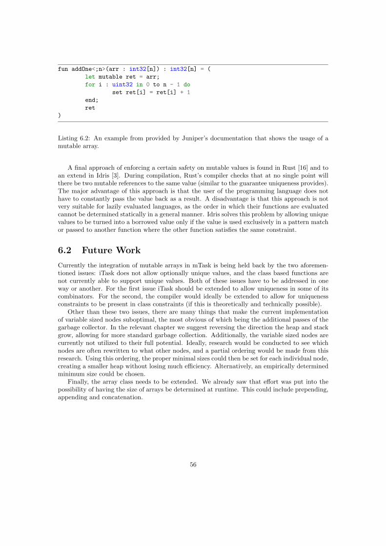
fun addOne<;n>(arr : int32[n]) : int32[n] = (

let mutable ret = arr;

for i : uint32 in 0 to n - 1 do

set ret[i] = ret[i] + 1

end;

ret

)

Listing 6.2: An example from provided by Juniper’s documentation that shows the usage of amutable array.

A final approach of enforcing a certain safety on mutable values is found in Rust [16] and toan extend in Idris [3]. During compilation, Rust’s compiler checks that at no single point willthere be two mutable references to the same value (similar to the guarantee uniqueness provides).The major advantage of this approach is that the user of the programming language does nothave to constantly pass the value back as a result. A disadvantage is that this approach is notvery suitable for lazily evaluated languages, as the order in which their functions are evaluatedcannot be determined statically in a general manner. Idris solves this problem by allowing uniquevalues to be turned into a borrowed value only if the value is used exclusively in a pattern matchor passed to another function where the other function satisfies the same constraint.

6.2 Future Work

Currently the integration of mutable arrays in mTask is being held back by the two aforemen-tioned issues: iTask does not allow optionally unique values, and the class based functions arenot currently able to support unique values. Both of these issues have to be addressed in oneway or another. For the first issue iTask should be extended to allow uniqueness in some of itscombinators. For the second, the compiler would ideally be extended to allow for uniquenessconstraints to be present in class constraints (if this is theoretically and technically possible).

Other than these two issues, there are many things that make the current implementationof variable sized nodes suboptimal, the most obvious of which being the additional passes of thegarbage collector. In the relevant chapter we suggest reversing the direction the heap and stackgrow, allowing for more standard garbage collection. Additionally, the variable sized nodes arecurrently not utilized to their full potential. Ideally, research would be conducted to see whichnodes are often rewritten to what other nodes, and a partial ordering would be made from thisresearch. Using this ordering, the proper minimal sizes could then be set for each individual node,creating a smaller heap without losing much efficiency. Alternatively, an empirically determinedminimum size could be chosen.

Finally, the array class needs to be extended. We already saw that effort was put into thepossibility of having the size of arrays be determined at runtime. This could include prepending,appending and concatenation.

56

Bibliography

[1] Ole Agesen and David Detlefs. Finding references in java stacks. In Proceedings of theOOPSLA’97 Workshop on Garbage Collection and Memory Management, 1997.

[2] Erik Barendsen and Sjaak Smetsers. Conventional and uniqueness typing in graph rewritesystems. In International Conference on Foundations of Software Technology and TheoreticalComputer Science, pages 41–51. Springer, 1993.

[3] Edwin Brady. Idris, a general-purpose dependently typed programming language: Designand implementation. Journal of functional programming, 23(5):552–593, 2013.

[4] Edwin Brady. ConcIO. https://github.com/edwinb/ConcIO, 2015.

[5] Loe Feijs. Multi-tasking and arduino: why and how? Design and semantics of form andmovement, 119, 2013.

[6] Mark Grebe and Andy Gill. Haskino: A remote monad for programming the arduino.In International Symposium on Practical Aspects of Declarative Languages, pages 153–168.Springer, 2016.

[7] Clemens Grelck and Sven-Bodo Scholz. Sac—a functional array language for efficient multi-threaded execution. International Journal of Parallel Programming, 34(4):383–427, 2006.

[8] Caleb Helbling and Samuel Z Guyer. Juniper: a functional reactive programming languagefor the arduino. In Proceedings of the 4th International Workshop on Functional Art, Music,Modelling, and Design, pages 8–16, 2016.

[9] Troels Henriksen, Niels GW Serup, Martin Elsman, Fritz Henglein, and Cosmin E Oancea.Futhark: purely functional gpu-programming with nested parallelism and in-place arrayupdates. In Proceedings of the 38th ACM SIGPLAN Conference on Programming LanguageDesign and Implementation, pages 556–571, 2017.

[10] Joey Hess. arduino-copilot: Arduino programming in haskell using the copilot streamdsl. hackage.haskell.org/package/arduino-copilot, 2020.

[11] Johan Jeuring, Patrik Jansson, and Claudio Amaral. Testing type class laws. In Proceedingsof the 2012 Haskell Symposium, pages 49–60, 2012.

[12] Rickard Lindberg. frp-arduino: Arduino programming without the hassle of c. hackage.haskell.org/package/frp-arduino, 2018.

[13] H.J. Lu, Matz Michael, Milind Girkar, Jan Hubicka, Andreas Jaeger, and Mark Mitchell.System V Application Binary Interface, 2018.

57

https://github.com/edwinb/ConcIO

hackage.haskell.org/package/arduino-copilot

hackage.haskell.org/package/frp-arduino

hackage.haskell.org/package/frp-arduino

[14] Mart Lubbers, Pieter Koopman, and Rinus Plasmeijer. Multitasking on microcontrollersusing task oriented programming. In 2019 42nd International Convention on Informationand Communication Technology, Electronics and Microelectronics (MIPRO), pages 1587–1592. IEEE, 2019.

[15] Geoffrey Mainland and Greg Morrisett. Nikola: embedding compiled gpu functions inhaskell. In Proceedings of the third ACM Haskell symposium on Haskell, pages 67–78, 2010.

[16] Nicholas D Matsakis and Felix S Klock. The Rust language. ACM SIGAda Ada Letters,34(3):103–104, 2014.

[17] Steffen Michels and Rinus Plasmeijer. Uniform data sources in a functional language. InSubmitted for presentation at Symposium on Trends in Functional Programming, TFP, vol-ume 12, 2012.

[18] Jennifer Paykin and Steve Zdancewic. The linearity monad. ACM SIGPLAN Notices,52(10):117–132, 2017.

[19] Rinus Plasmeijer, Bas Lijnse, Steffen Michels, Peter Achten, and Pieter Koopman. Task-oriented programming in a pure functional language. In Proceedings of the 14th symposiumon Principles and practice of declarative programming, pages 195–206, 2012.

[20] Philip Wadler. Monads for functional programming. In International School on AdvancedFunctional Programming, pages 24–52. Springer, 1995.

58

Appendices

59

Appendix A

Monad Laws Proof for the MaybeMonad

Left Identity:

return a >>= k

= (Just a) >>= k

= k a

Right Identity:

m >>= return

case 1: m = Just x

= (Just x) >>= return

= return x

= Just x

= m

case 2: m = Nothing

= Nothing >>= return

= Nothing

= m

Associativity:

m >>= (\x -> k x >>= h)

= m >>= (\x -> case k x of

Nothing -> Nothing

Just x -> h x)

case 1: m = Nothing

= Nothing >>= (\x -> case k x of

Nothing -> Nothing

Just x -> h x)

= Nothing

= Nothing >>= h

= (Nothing >>= k) >>= h

60

= (m >>= k) >>= h

case 2: m = Just a

= Just a >>= (\x -> case k x of

Nothing -> Nothing

Just x -> h x)

= (\x -> case k x of

Nothing -> Nothing

Just x -> h x) a

= case k a of

Nothing -> Nothing

Just x -> h x

case 1: k a = Nothing

= Nothing

= Nothing >>= h

= k a >>= h

= (Just a >>= k) >>= h

= (m >>= k) >>= h

case 2: k a = Just b

= h b

= Just b >>= h

= k a >>= h

= (Just a >>= k) >>= h

= (m >>= k) >>= h

61

Appendix B

A Unique If Function

module if

// ALLOWED


f b i = if b i i

// NOT ALLOWED

g :: Bool *Int -> *Int

g b i = my_if b i i

where


my_if b t e = if b t e

h :: Bool *Int -> *Int

h b i = my_if b i i

where


my_if True t _ = t

my_if _ _ e = e

k :: Bool *Int -> *Int

k b i = my_if b i i

where


my_if b t e

| b = t

| otherwise = e

Start =

[ f True uniqueInt

, g True uniqueInt

, h True uniqueInt

, k True uniqueInt

62

]

where

uniqueInt :: *Int

uniqueInt = 42

63

Appendix C

Moving Average

C.1 Non-Unique

DHT D1 DHT11 \dht->

sds \avg=0 In


If (i >=. lit 10) (

acc /. lit 10

) (


)

) In


delay (lit 1000)


>>~. \v



= sdsSet avg x

>>|. If (i <. 9)



) In

fun \act=(\on->

getSds avg

>>*.



]

>>=. act

) In



64

C.2 Unique With If Problem

DHT D1 DHT11 \dht->

sds \avg=0 In


If (i >=. lit 10) (


) (



)

) In


delay (lit 1000)


>>~. \v



= sdsSet avg x

>>|. If (i <. 9)



) In

fun \act=(\on->

getSds avg

>>*.



]

>>=. act

) In



C.3 Unique Without If Problem

DHT D1 DHT11 \dht->

sds \avg=0 In


If (i >=. lit 10) (


) (



)

) In


65

delay (lit 1000)


>>~. \v



= sdsSet avg x

>>=. \_

# i = If (i <. 9) (i +. lit 1) (lit 0)

= measure (i, arr)

) In

fun \act=(\on->

getSds avg

>>*.


true)↪→


]

>>=. act

) In



66

Mutable Collection Types in Shallow Embedded DSLs

Documents

Transcript of Mutable Collection Types in Shallow Embedded DSLs