Music in Our Ears: The Biological Bases of Musical Timbre ... · Music in Our Ears: The Biological...
16
Music in Our Ears: The Biological Bases of Musical Timbre Perception Kailash Patil 1 , Daniel Pressnitzer 2 , Shihab Shamma 3 , Mounya Elhilali 1 * 1 Department of Electrical and Computer Engineering, Center for Language and Speech Processing, Johns Hopkins University, Baltimore, Maryland, United States of America, 2 Laboratoire Psychologie de la Perception, CNRS-Universite ´ Paris Descartes & DEC, Ecole normale supe ´ rieure, Paris, France, 3 Department of Electrical and Computer Engineering and Institute for Systems Research, University of Maryland, College Park, Maryland, United States of America Abstract Timbre is the attribute of sound that allows humans and other animals to distinguish among different sound sources. Studies based on psychophysical judgments of musical timbre, ecological analyses of sound’s physical characteristics as well as machine learning approaches have all suggested that timbre is a multifaceted attribute that invokes both spectral and temporal sound features. Here, we explored the neural underpinnings of musical timbre. We used a neuro-computational framework based on spectro-temporal receptive fields, recorded from over a thousand neurons in the mammalian primary auditory cortex as well as from simulated cortical neurons, augmented with a nonlinear classifier. The model was able to perform robust instrument classification irrespective of pitch and playing style, with an accuracy of 98.7%. Using the same front end, the model was also able to reproduce perceptual distance judgments between timbres as perceived by human listeners. The study demonstrates that joint spectro-temporal features, such as those observed in the mammalian primary auditory cortex, are critical to provide the rich-enough representation necessary to account for perceptual judgments of timbre by human listeners, as well as recognition of musical instruments. Citation: Patil K, Pressnitzer D, Shamma S, Elhilali M (2012) Music in Our Ears: The Biological Bases of Musical Timbre Perception. PLoS Comput Biol 8(11): e1002759. doi:10.1371/journal.pcbi.1002759 Editor: Frederic E. Theunissen, University of California at Berkeley, United States of America Received March 23, 2012; Accepted September 12, 2012; Published November 1, 2012 Copyright: ß 2012 Patil et al. This is an open-access article distributed under the terms of the Creative Commons Attribution License, which permits unrestricted use, distribution, and reproduction in any medium, provided the original author and source are credited. Funding: This work was partly supported by grants from NSF CAREER IIS-0846112, AFOSR FA9550-09-1-0234, NIH 1R01AG036424-01 and ONR N000141010278. S. Shamma was partly supported by a Blaise-Pascal Chair, Re ´gion Ile de France, and by the program Research in Paris, Mairie de Paris. The funders had no role in study design, data collection and analysis, decision to publish, or preparation of the manuscript. Competing Interests: The authors have declared that no competing interests exist. * E-mail: [email protected] Introduction A fundamental role of auditory perception is to infer the likely source of a sound; for instance to identify an animal in a dark forest, or to recognize a familiar voice on the phone. Timbre, often referred to as the color of sound, is believed to play a key role in this recognition process [1]. Though timbre is an intuitive concept, its formal definition is less so. The ANSI definition of timbre describes it as that attribute that allows us to distinguish between sounds having the same perceptual duration, loudness, and pitch, such as two different musical instruments playing exactly the same note [2]. In other words, it is neither duration, nor loudness, nor pitch; but is likely ‘‘everything else’’. As has been often been pointed out, this definition by the negative does not state what are the perceptual dimensions underlying timbre perception. Spectrum is obviously a strong candidate: physical objects produce sounds with a spectral profile that reflects their particular sets of vibration modes and resonances [3]. Measures of spectral shape have thus been proposed as basic dimensions of timbre (e.g., formant position for voiced sounds in speech, sharpness, and brightness) [4,5]. But timbre is not only spectrum, as changes of amplitude over time, the so-called temporal envelope, also have strong perceptual effects [6,7]. To identify the most salient timbre dimensions, statistical techniques such as multidimensional scaling have been used: perceptual differences between sound samples were collected and the underlying dimensionality of the timbre space inferred [8,9]. These studies suggest a combination of spectral and temporal dimensions to explain the perceptual distance judgments, but the precise nature of these dimensions varies across studies and sound sets [10,11]. Importantly, almost all timbre dimensions that have been proposed to date on the basis of psychophysical studies [12] are either purely spectral or purely temporal. The only spectro- temporal aspect of sound that has been considered in this context is related to the asynchrony of partials around the onset of a sound (8,9), but the salience of this spectro-temporal dimension was found to be weak and context-dependent [13]. Technological approaches, not concerned with biology nor human perception, have explored much richer feature represen- tations that span both spectral, temporal, and spectro-temporal dimensions. The motivation for these engineering techniques is an accurate recognition of specific sounds or acoustic events in a variety of applications (e.g. automatic speech recognition; voice detection; music information retrieval; target tracking in multi- sensor networks and surveillance systems; medical diagnosis, etc.). Myriad spectral features have been proposed for audio content analysis, ranging from simple summary statistics of spectral shape (e.g. spectral amplitude, peak, centroid, flatness) to more elaborate descriptions of spectral information such as Mel-Frequency Cepstral Coefficients (MFCC) and Linear or Perceptual Predictive Coding (LPC or PLP) [14–16]. Such metrics have often been augmented with temporal information, which was found to improve the robustness of content identification [17,18]. Common modeling of temporal dynamics also ranged from simple summary PLOS Computational Biology | www.ploscompbiol.org 1 November 2012 | Volume 8 | Issue 11 | e1002759
Transcript of Music in Our Ears: The Biological Bases of Musical Timbre ... · Music in Our Ears: The Biological...
Music in Our Ears: The Biological Bases of Musical TimbrePerceptionKailash Patil1, Daniel Pressnitzer2, Shihab Shamma3, Mounya Elhilali1*
1 Department of Electrical and Computer Engineering, Center for Language and Speech Processing, Johns Hopkins University, Baltimore, Maryland, United States of
America, 2 Laboratoire Psychologie de la Perception, CNRS-Universite Paris Descartes & DEC, Ecole normale superieure, Paris, France, 3 Department of Electrical and
Computer Engineering and Institute for Systems Research, University of Maryland, College Park, Maryland, United States of America
Abstract
Timbre is the attribute of sound that allows humans and other animals to distinguish among different sound sources.Studies based on psychophysical judgments of musical timbre, ecological analyses of sound’s physical characteristics as wellas machine learning approaches have all suggested that timbre is a multifaceted attribute that invokes both spectral andtemporal sound features. Here, we explored the neural underpinnings of musical timbre. We used a neuro-computationalframework based on spectro-temporal receptive fields, recorded from over a thousand neurons in the mammalian primaryauditory cortex as well as from simulated cortical neurons, augmented with a nonlinear classifier. The model was able toperform robust instrument classification irrespective of pitch and playing style, with an accuracy of 98.7%. Using the samefront end, the model was also able to reproduce perceptual distance judgments between timbres as perceived by humanlisteners. The study demonstrates that joint spectro-temporal features, such as those observed in the mammalian primaryauditory cortex, are critical to provide the rich-enough representation necessary to account for perceptual judgments oftimbre by human listeners, as well as recognition of musical instruments.
Citation: Patil K, Pressnitzer D, Shamma S, Elhilali M (2012) Music in Our Ears: The Biological Bases of Musical Timbre Perception. PLoS Comput Biol 8(11):e1002759. doi:10.1371/journal.pcbi.1002759
Editor: Frederic E. Theunissen, University of California at Berkeley, United States of America
Received March 23, 2012; Accepted September 12, 2012; Published November 1, 2012
Copyright: � 2012 Patil et al. This is an open-access article distributed under the terms of the Creative Commons Attribution License, which permits unrestricteduse, distribution, and reproduction in any medium, provided the original author and source are credited.
Funding: This work was partly supported by grants from NSF CAREER IIS-0846112, AFOSR FA9550-09-1-0234, NIH 1R01AG036424-01 and ONR N000141010278. S.Shamma was partly supported by a Blaise-Pascal Chair, Region Ile de France, and by the program Research in Paris, Mairie de Paris. The funders had no role instudy design, data collection and analysis, decision to publish, or preparation of the manuscript.
Competing Interests: The authors have declared that no competing interests exist.
* E-mail: [email protected]
Introduction
A fundamental role of auditory perception is to infer the likely
source of a sound; for instance to identify an animal in a dark
forest, or to recognize a familiar voice on the phone. Timbre, often
referred to as the color of sound, is believed to play a key role in
this recognition process [1]. Though timbre is an intuitive concept,
its formal definition is less so. The ANSI definition of timbre
describes it as that attribute that allows us to distinguish between
sounds having the same perceptual duration, loudness, and pitch,
such as two different musical instruments playing exactly the same
note [2]. In other words, it is neither duration, nor loudness, nor
pitch; but is likely ‘‘everything else’’.
As has been often been pointed out, this definition by the
negative does not state what are the perceptual dimensions
underlying timbre perception. Spectrum is obviously a strong
candidate: physical objects produce sounds with a spectral profile
that reflects their particular sets of vibration modes and resonances
[3]. Measures of spectral shape have thus been proposed as basic
dimensions of timbre (e.g., formant position for voiced sounds in
speech, sharpness, and brightness) [4,5]. But timbre is not only
spectrum, as changes of amplitude over time, the so-called
temporal envelope, also have strong perceptual effects [6,7]. To
identify the most salient timbre dimensions, statistical techniques
such as multidimensional scaling have been used: perceptual
differences between sound samples were collected and the
underlying dimensionality of the timbre space inferred [8,9].
These studies suggest a combination of spectral and temporal
dimensions to explain the perceptual distance judgments, but the
precise nature of these dimensions varies across studies and sound
sets [10,11]. Importantly, almost all timbre dimensions that have
been proposed to date on the basis of psychophysical studies [12]
are either purely spectral or purely temporal. The only spectro-
temporal aspect of sound that has been considered in this context
is related to the asynchrony of partials around the onset of a sound
(8,9), but the salience of this spectro-temporal dimension was
found to be weak and context-dependent [13].
Technological approaches, not concerned with biology nor
human perception, have explored much richer feature represen-
tations that span both spectral, temporal, and spectro-temporal
dimensions. The motivation for these engineering techniques is an
accurate recognition of specific sounds or acoustic events in a
variety of applications (e.g. automatic speech recognition; voice
detection; music information retrieval; target tracking in multi-
sensor networks and surveillance systems; medical diagnosis, etc.).
Myriad spectral features have been proposed for audio content
analysis, ranging from simple summary statistics of spectral shape
(e.g. spectral amplitude, peak, centroid, flatness) to more elaborate
descriptions of spectral information such as Mel-Frequency
Cepstral Coefficients (MFCC) and Linear or Perceptual Predictive
Coding (LPC or PLP) [14–16]. Such metrics have often been
augmented with temporal information, which was found to
improve the robustness of content identification [17,18]. Common
modeling of temporal dynamics also ranged from simple summary
PLOS Computational Biology | www.ploscompbiol.org 1 November 2012 | Volume 8 | Issue 11 | e1002759
statistics such as onsets, attack time, velocity, acceleration and
higher-order moments to more sophisticated statistical temporal
modeling using Hidden Markov Models, Artificial Neural
Networks, Adaptive Resonance Theory models, Liquid State
Machine systems and Self-Organizing Maps [19,20]. Overall, the
choice of features was very dependent on the task at hand, the
complexity of the dataset, and the desired performance level and
robustness of the system.
Complementing perceptual and technological approaches,
brain-imaging techniques have been used to explore the neural
underpinnings of timbre perception. Correlates of musical timbre
dimensions suggested by multidimensional scaling studies have
been observed using event-related potentials [21]. Other studies
have attempted to identify the neural substrates of natural sound
recognition, by looking for brain areas that would be selective to
specific sound categories, such as voice-specific regions in
secondary cortical areas [22,23] and other sound categories such
as tools [24] or musical instruments [25]. A hierarchical model
consistent with these findings has been proposed in which
selectivity to different sound categories is refined as one climbs
the processing chain [26]. An alternative, more distributed scheme
has also been suggested [27,28], which includes the contribution of
low-level cues to the large perceptual differences between these
high-level sound categories.
A common issue for the psychophysical, technological, and
neurophysiological investigations of timbre is that the generality of
the results is mitigated by the particular characteristics of the
sound set used. For multi-dimensional scaling behavioral studies,
by construction, the dimensions found will be the most salient
within the sound set; but they may not capture other dimensions
which could nevertheless be crucial for the recognition of sounds
outside the set. For engineering studies, dimensions may be
designed arbitrarily as long as they afford good performance in a
specific task. For the imaging studies, there is no suggestion yet as
to which low-level acoustic features may be used to construct the
various selectivity for high-level categories while preserving
invariance within a category. Furthermore, there is a major gap
between these studies and what is known from electrophysiological
recordings in animal models. Decades of work have established
that auditory cortical responses display rich and complex spectro-
temporal receptive fields, even within primary areas [29,30]. This
seems at odds with the limited set of spectral or temporal
dimensions that are classically used to characterize timbre in
perceptual studies.
To bridge this gap, we investigate how cortical processing of
spectro-temporal modulations can subserve both sound source
recognition of musical instruments and perceptual timbre judg-
ments. Specifically, cortical receptive fields and computational
models derived from them are shown to be suited to classify a
sound source from its evoked neural activity, across a wide range
of instruments, pitches and playing styles, and also to predict
accurately human judgments of timbre similarities
Results
Cortical processing of complex musical soundsResponses in primary auditory cortex (A1) exhibit rich
selectivity that extends beyond the tonotopy observed in the
auditory nerve. A1 neurons are not only tuned to the spectral
energy at a given frequency, but also to the specifics of the local
spectral shape such as its bandwidth [31], spectral symmetry [32],
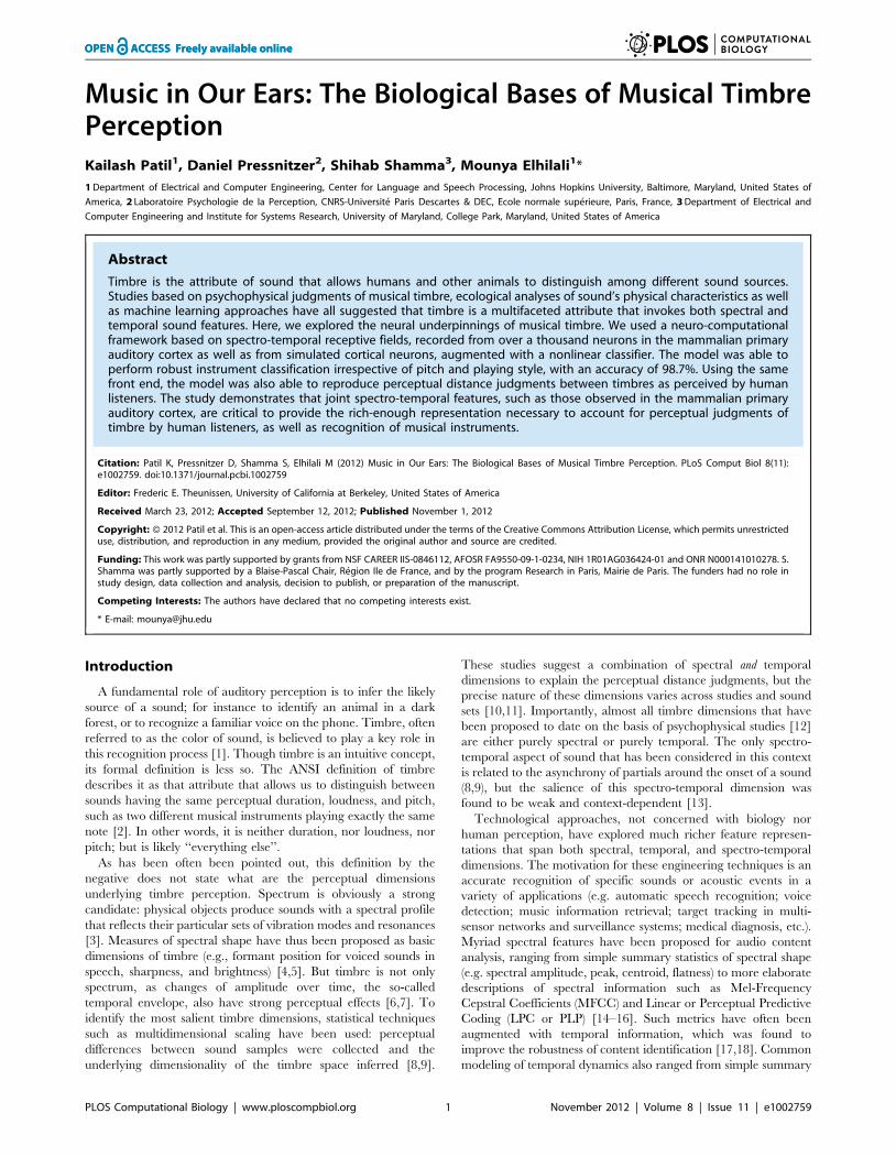
and temporal dynamics [33] (Figure 1). Put together, one can view
the resulting representation of sound in A1 as a multidimensional
mapping that spans at least three dimensions: (1) Best frequencies that
span the entire auditory range; (2) Spectral shapes (including
bandwidth and symmetry) that span a wide range from very
broad (2–3 octaves) to narrowly tuned (,0.25 octaves); and (3)
Dynamics that range from very slow to relatively fast (1–30 Hz).
This rich cortical mapping may reflect an elegant strategy for
extracting acoustic cues that subserve the perception of various
acoustic attributes (pitch, loudness, location, and timbre) as well as
the recognition of complex sound objects, such as different musical
instruments. This hypothesis was tested here by employing a
database of spectro-temporal receptive fields (STRFs) recorded
from 1110 single units in primary auditory cortex of 15 awake
non-behaving ferrets. These receptive fields are linear descriptors of
the selectivity of each cortical neuron to the spectral and temporal
modulations evident in the cochlear ‘‘spectrogram-like’’ represen-
tation of complex acoustic signals that emerges in the auditory
periphery. Such STRFs (with a variety of nonlinear refinements)
have been shown to capture and predict well cortical responses to
a variety of complex sounds like speech, music, and modulated
noise [34–38].
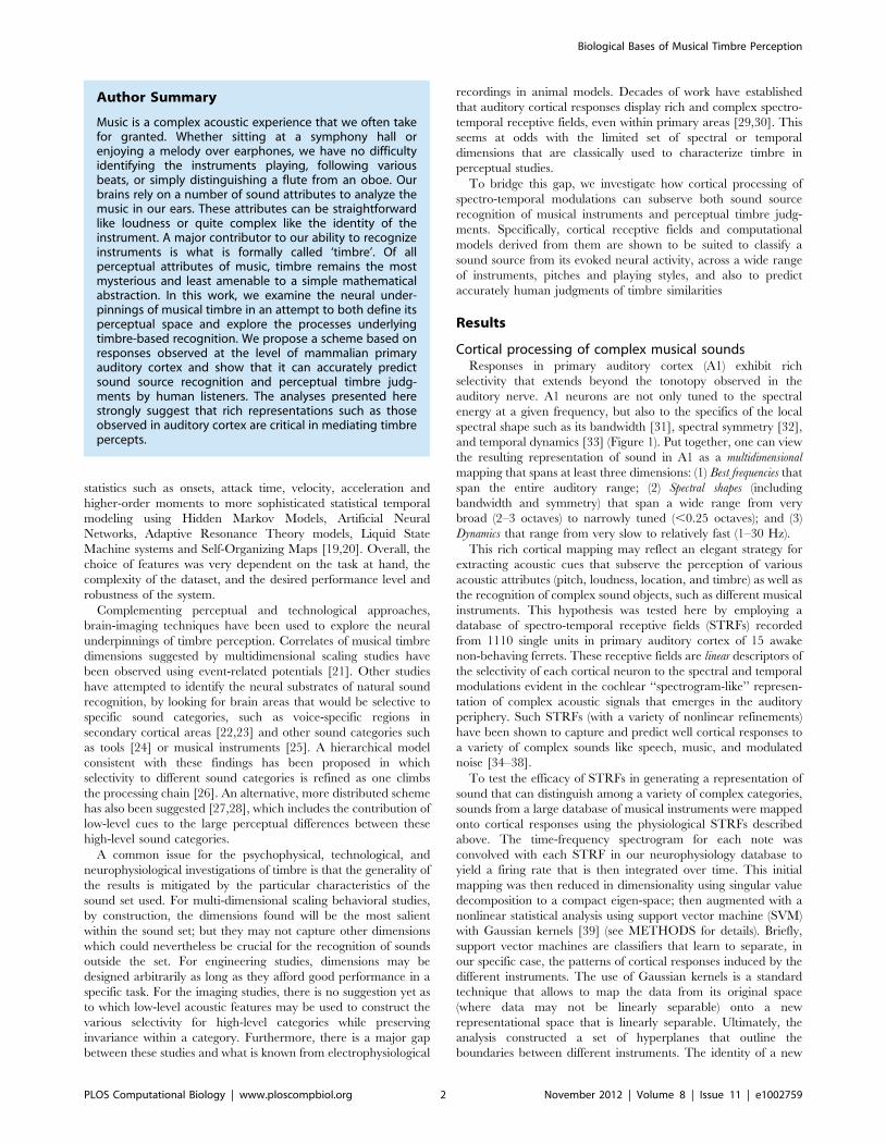
To test the efficacy of STRFs in generating a representation of
sound that can distinguish among a variety of complex categories,
sounds from a large database of musical instruments were mapped
onto cortical responses using the physiological STRFs described
above. The time-frequency spectrogram for each note was
convolved with each STRF in our neurophysiology database to
yield a firing rate that is then integrated over time. This initial
mapping was then reduced in dimensionality using singular value
decomposition to a compact eigen-space; then augmented with a
nonlinear statistical analysis using support vector machine (SVM)
with Gaussian kernels [39] (see METHODS for details). Briefly,
support vector machines are classifiers that learn to separate, in
our specific case, the patterns of cortical responses induced by the
different instruments. The use of Gaussian kernels is a standard
technique that allows to map the data from its original space
(where data may not be linearly separable) onto a new
representational space that is linearly separable. Ultimately, the
analysis constructed a set of hyperplanes that outline the
boundaries between different instruments. The identity of a new
Author Summary
Music is a complex acoustic experience that we often takefor granted. Whether sitting at a symphony hall orenjoying a melody over earphones, we have no difficultyidentifying the instruments playing, following variousbeats, or simply distinguishing a flute from an oboe. Ourbrains rely on a number of sound attributes to analyze themusic in our ears. These attributes can be straightforwardlike loudness or quite complex like the identity of theinstrument. A major contributor to our ability to recognizeinstruments is what is formally called ‘timbre’. Of allperceptual attributes of music, timbre remains the mostmysterious and least amenable to a simple mathematicalabstraction. In this work, we examine the neural under-pinnings of musical timbre in an attempt to both define itsperceptual space and explore the processes underlyingtimbre-based recognition. We propose a scheme based onresponses observed at the level of mammalian primaryauditory cortex and show that it can accurately predictsound source recognition and perceptual timbre judg-ments by human listeners. The analyses presented herestrongly suggest that rich representations such as thoseobserved in auditory cortex are critical in mediating timbrepercepts.
Biological Bases of Musical Timbre Perception
PLOS Computational Biology | www.ploscompbiol.org 2 November 2012 | Volume 8 | Issue 11 | e1002759
sample was then defined based on its configuration in this
expanded space relative to the set of learned hyperplanes
(Figure 2).
Based on the configuration above and a 10% cross-validation
technique, the model trained using the physiological cortical
receptive fields achieved a classification accuracy of
87.22%±0.81 (the number following the mean accuracy
represents standard deviation, see Table 1). Remarkably, this
result was obtained with a large database of 11 instruments playing
between 30 and 90 different pitches with 3 to 19 playing styles
(depending on the instrument), 3 style dynamics (mezzo, forte and
piano), and 3 manufacturers for each instrument (an average of
1980 notes/instrument). This high classification accuracy was a
strong indicator that neural processing at the level of primary
auditory cortex could not only provide a basis for distinguishing
between different instruments, but also had a robust invariant
representation of instruments over a wide range of pitches and
playing styles.
The cortical modelDespite the encouraging results obtained using cortical receptive
fields, the classification based on neurophysiological recordings
was hampered by various shortcomings including recording noise
and other experimental constraints. Also, the limited selection of
receptive fields (being from ferrets) tended to under-represent
parameter ranges relevant to humans such as lower frequencies,
narrow bandwidths (limited to a maximum resolution of 1.2
octaves), and coarse sampling of STRF dynamics.
To circumvent these biases, we employed a model that mimics
the basic transformations along the auditory pathway up to the
level of A1. Effectively, the model mapped the one-dimensional
acoustic waveform onto a multidimensional feature space.
Importantly, the model allowed us to sample the cortical space
more uniformly than physiological data available to us, in line with
findings in the literature [29,30,40].
The model operates by first mapping the acoustic signal into an
auditory spectrogram. This initial transformation highlights the
time varying spectral energies of different instruments which is at
Figure 1. Neurophysiological receptive fields. Each panel shows the receptive field of 1 neuron with red indicating excitatory (preferred)responses, and blue indicating inhibitory (suppressed) responses. Examples vary from narrowly tuned neurons (top row) to broadly tuned ones(middle and bottom row). They also highlight variability in temporal dynamics and orientation (upward or downward sweeps).doi:10.1371/journal.pcbi.1002759.g001
Figure 2. Schematic of the timbre recognition model. An acoustic waveform from a test instrument is processed through a model of cochlearand midbrain processing; yielding a time-frequency representation called auditory spectrogram. This later is further processed through the corticalprocessing stage through neurophysiological or model spectro-temporal receptive fields. Cortical responses of the target instrument are testedagainst boundaries of a statistical SVM timbre model in order to identify the instrument’s identity.doi:10.1371/journal.pcbi.1002759.g002
Biological Bases of Musical Timbre Perception
PLOS Computational Biology | www.ploscompbiol.org 3 November 2012 | Volume 8 | Issue 11 | e1002759
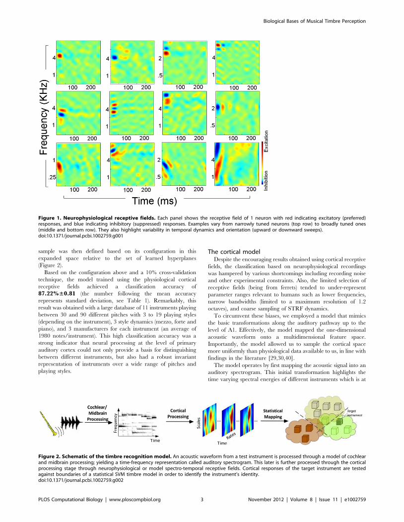
the core of most acoustic correlates and machine learning analyses
of musical timbre [5,11,13,41,42]. For instance, temporal features
in a musical note include fast dynamics that reflect the quality of
the sound (scratchy, whispered, or purely voiced), as well as slower
modulations that carry nuances of musical timbre such as attack
and decay times, subtle fluctuations of pitch (vibrato) or amplitude
(shimmer). Some of these characteristics can be readily seen in the
auditory spectrograms, but many are only implicitly represented.
For example, Figure 3A contrasts the auditory spectrogram of a
piano vs. violin note. For violin, the temporal cross-section reflects
the soft onset and sustained nature of bowing and typical vibrato
fluctuations; the spectral slice captures the harmonic structure of
the musical note with the overall envelope reflecting the
resonances of the violin body. By contrast, the temporal and
spectral modulations of a piano (playing the same note) are quite
different. Temporally, the onset of piano rises and falls much
faster, and its spectral envelope is much smoother.
The cortical stage of the auditory model further analyzes the
spectral and temporal modulations of the spectrogram along
multiple spectral and temporal resolutions. The model projects the
auditory spectrogram onto a 4-dimensional space, representing
time, tonotopic frequency, spectral modulations (or scales) and
temporal modulations (or rates). The four dimensions of the
cortical output can be interpreted in various ways. In one view, the
cortical model output is a parallel repeated representation of the
auditory spectrogram viewed at different resolutions. A different
view is one of a bank of spectral and temporal modulation filters
with different tuning (from narrowband to broadband spectrally,
Table 1. Classification performance for the different models.
Mean STD
Auditory Spectrum (Gaussian kernel SVM) 79.1% 0.7%
Neurophysiological STRFs (Gaussian kernel SVM) 87.2% 0.8%
Full Cortical Model (Linear SVM) 96.2% 0.5%
Full Cortical Model (Gaussian kernel SVM) 98.7% 0.2%
The middle column indicates the mean of the accuracy scores for the 10 foldcross validation experiment and the right column indicates their standarddeviation. Models differ either in their feature set (e.g. full cortical model versusauditory spectrogram) or in the classifier used (linear SVM versus Gaussiankernel SVM).doi:10.1371/journal.pcbi.1002759.t001
Figure 3. Spectro-temporal modulation profiles highlighting timbre differences between piano and violin notes. (A) The plot showsthe time-frequency auditory spectrogram of piano and violin notes. The temporal and spectral slices shown on the right are marked. (B) The plotsshow magnitude cortical responses of four piano notes (left panels), played in normal (left) and Staccato (right) at F4 (top) and F#4 (bottom); andfour violin notes (right panels), played in normal (left) and Pizzicatto (right) also at pitch F4(top) and F#4 (bottom). The white asterisks (upperleftmost notes in each quadruplet) indicate the notes shown in part (A) of this figure.doi:10.1371/journal.pcbi.1002759.g003
Biological Bases of Musical Timbre Perception
PLOS Computational Biology | www.ploscompbiol.org 4 November 2012 | Volume 8 | Issue 11 | e1002759
and slow to fast modulations temporally). In such view, the cortical
representation is a display of spectro-temporal modulations of each
channel as they evolve over time. Ultimately each filter acts as a
model cortical neuron whose output reflects the tuning of that
neuronal site. The model employed here had 30,976 filters
(128freq622 rates611 scales), hence allowing us to obtain a full
uniform coverage of the cortical space and bypassing the
limitations of neurophysiological data. Note that we are not
suggesting that ,30 K neurons are needed for timbre classifica-
tion, as the feature space is reduced in further stages of the model
(see below). We have not performed an analysis of the number of
neurons needed for such task. Nonetheless, a large and uniform
sampling of the space seemed desirable.
By collapsing the cortical display over frequency and
averaging over time, one would obtain a two-dimensional
display that preserves the ‘‘global’’ distribution of modulations
over the remaining two dimensions of scale and rates. This
‘‘scale-rate’’ view is shown in Figure 3B for the same piano and
violin notes in Figure 3A as well as others. Each instrument here
is played at two distinct pitches with two different playing styles.
The panels provide estimates of the overall distribution of
spectro-temporal modulation of each sound. The left panel
highlights the fact that the violin vibrato concentrates its peak
energy near 6 Hz (across all pitches and styles); which matches
the speed of pulsating pitch change caused by the rhythmic rate
of 6 pulses per second chosen for the vibrato of this violin note.
By contrast, the rapid onset of piano distributes its energy across
a wider range of temporal modulations. Similarly, the unique
pattern of peaks and valleys in spectral envelopes of each
instrument produces a broad distribution along the spectral
modulation axis, with the violin’s sharper spectral peaks
activating higher spectral modulations while the piano’s
smoother profile activates broad bandwidths. Each instrument,
therefore, produces a correspondingly unique spectro-temporal
activation pattern that could potentially be used to recognize it
or distinguish it from others.
Musical timbre classificationSeveral computational models were compared in the same
classification task analysis of the database of musical instruments as
described earlier with real neurophysiological data. Results
comparing all models are summarized in Table 1. For what we
refer to as the full model, we used the 4-D cortical model. The
analysis started with a linear mapping through the model receptive
fields, followed by dimensionality reduction and statistical
classification using support vector machines with re-optimized
Gaussian kernels (see Methods). Tests used a 10% cross-validation
method. The cortical model yielded an excellent classification
accuracy of 98.7%±0.2.
We also explored the use of linear support vector machine, by
bypassing the use of the Gaussian kernel. We performed a
classification of instruments using the cortical responses obtained
from the model receptive fields and a linear SVM. After
optimization of the decision boundaries, we obtained an accuracy
of 96.2%±0.5. This result supports our initial assessment that the
cortical space does indeed capture most of the subtleties that are
unique to a common instrument but distinct between different
classes. It is mostly the richness of the representation that underlies
the classification performance: only a small improvement in
accuracy is observed by adding the non-linear warping in the full
model.
In order to better understand the contribution of the cortical
analysis beyond the time-frequency representation, we explored
reduced versions of the full model. First we performed the timbre
classification task using the auditory spectrogram as input. The
feature spectra were obtained by processing the time waveform of
each note through the cochlear-like filterbank front-end and
averaging the auditory spectrograms over time, yielding a one-
dimensional spectral profile for each note. These were then
processed through the same statistical SVM model, with
Gaussian functions optimized for this new representation using
the exact same methods as used for cortical features. The
classification accuracy for the spectral slices with SVM optimi-
zation attained a good but limited accuracy of 79.1%±0.7. It is
expected that a purely spectral model would not be able to
classify all instruments. Whereas basic instrument classes differing
by their physical characteristics (wind, percussion, strings) may
have the potential to produce different spectral shapes, preserved
in the spectral vector, more subtle differences in the temporal
domain should prove difficult to recognize on this basis (see
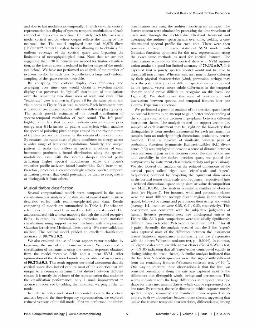
Figure 4). We shall revisit this issue of contribution and
interactions between spectral and temporal features later (see
Control Experiments section).
We performed a post-hoc analysis of the decision space based
on cortical features in an attempt to get a better understanding of
the configuration of the decision hyperplanes between different
instrument classes. The analysis treated the support vectors (i.e.
samples of each instrument that fall right on the boundary that
distinguishes it from another instrument) for each instrument as
samples from an underlying high-dimensional probability density
function. Then, a measure of similarity between pairs of
probability functions (symmetric Kullback–Leibler (KL) diver-
gence [43]) was employed to provide a sense of distance between
each instrument pair in the decision space. Because of the size
and variability in the timbre decision space, we pooled the
comparisons by instrument class (winds, strings and percussions).
We also focused our analysis on the reduced dimensions of the
cortical space; called ‘eigen’-rate, ‘eigen’-scale and ‘eigen’-
frequencies; obtained by projecting the equivalent dimensions
in the cortical tensor (rate, scale and frequency, respectively) into
a reduced dimensional space using singular-value decomposition
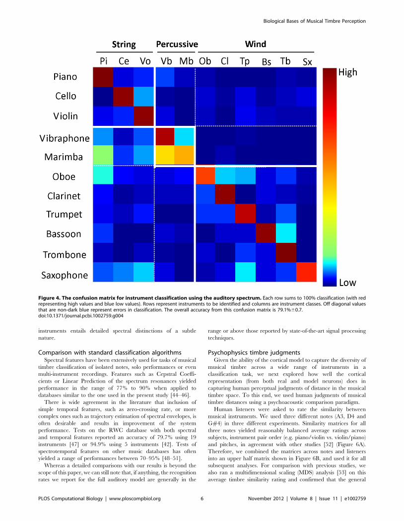
(see METHODS). The analysis revealed a number of observa-
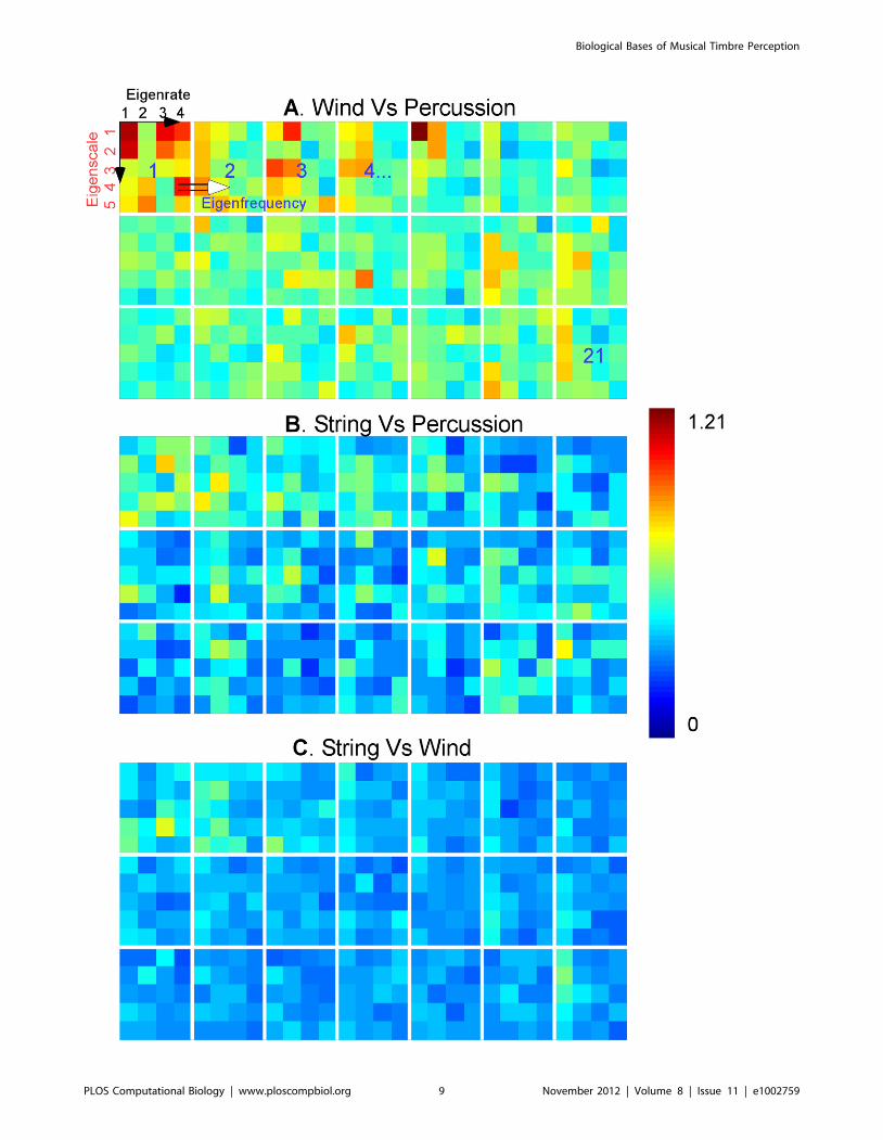
tions (see Figure 5). For instance, wind and percussion classes
were the most different (occupy distant regions in the decision
space), followed by strings and percussions then strings and winds
(average KL distances were 0.58, 0.41, 0.35, respectively). This
observation was consistent with the subjective judgments of
human listeners presented next (see off-diagonal entries in
Figure 6B). All 3 pair comparisons were statistically significantly
different from each other (Wilcoxon ranksum test, p,1025 for all
3 pairs). Secondly, the analysis revealed that the 2 first ‘eigen’-
rates captured most of the difference between the instrument
classes (statistical significance in comparing the first 2 eigenrates
with the others; Wilcoxon ranksum test, p = 0.0046). In contrast,
all ‘eigen’-scales were variable across classes (Kruskal-Wallis test,
p = 0.9185 indicating that all ‘eigen’-scales contributed equally in
distinguishing the broad classes). A similar analysis indicated that
the first four ‘eigen’-frequencies were also significantly different
from the remaining features (Wilcoxon ranksum test, p,1025).
One way to interpret these observations is that the first two
principal orientations along the rate axis captured most of the
differences that distinguish winds, strings and percussions. This
seems consistent with the large differences in temporal envelope
shape for these instruments classes, which can be represented by a
few rates. By contrast, the scale dimension (which captures mostly
spectral shape, symmetry and bandwidth) was required in its
entirety to draw a boundary between these classes, suggesting that
unlike the coarser temporal characteristics, differentiating among
Biological Bases of Musical Timbre Perception
PLOS Computational Biology | www.ploscompbiol.org 5 November 2012 | Volume 8 | Issue 11 | e1002759
instruments entails detailed spectral distinctions of a subtle
nature.
Comparison with standard classification algorithmsSpectral features have been extensively used for tasks of musical
timbre classification of isolated notes, solo performances or even
multi-instrument recordings. Features such as Cepstral Coeffi-
cients or Linear Prediction of the spectrum resonances yielded
performance in the range of 77% to 90% when applied to
databases similar to the one used in the present study [44–46].
There is wide agreement in the literature that inclusion of
simple temporal features, such as zero-crossing rate, or more
complex ones such as trajectory estimation of spectral envelopes, is
often desirable and results in improvement of the system
performance. Tests on the RWC database with both spectral
and temporal features reported an accuracy of 79.7% using 19
instruments [47] or 94.9% using 5 instruments [42]. Tests of
spectrotemporal features on other music databases has often
yielded a range of performances between 70–95% [48–51].
Whereas a detailed comparisons with our results is beyond the
scope of this paper, we can still note that, if anything, the recognition
rates we report for the full auditory model are generally in the
range or above those reported by state-of-the-art signal processing
techniques.
Psychophysics timbre judgmentsGiven the ability of the cortical model to capture the diversity of
musical timbre across a wide range of instruments in a
classification task, we next explored how well the cortical
representation (from both real and model neurons) does in
capturing human perceptual judgments of distance in the musical
timbre space. To this end, we used human judgments of musical
timbre distances using a psychoacoustic comparison paradigm.
Human listeners were asked to rate the similarity between
musical instruments. We used three different notes (A3, D4 and
G#4) in three different experiments. Similarity matrices for all
three notes yielded reasonably balanced average ratings across
subjects, instrument pair order (e.g. piano/violin vs. violin/piano)
and pitches, in agreement with other studies [52] (Figure 6A).
Therefore, we combined the matrices across notes and listeners
into an upper half matrix shown in Figure 6B, and used it for all
subsequent analyses. For comparison with previous studies, we
also ran a multidimensional scaling (MDS) analysis [53] on this
average timbre similarity rating and confirmed that the general
Figure 4. The confusion matrix for instrument classification using the auditory spectrum. Each row sums to 100% classification (with redrepresenting high values and blue low values). Rows represent instruments to be identified and columns are instrument classes. Off diagonal valuesthat are non-dark blue represent errors in classification. The overall accuracy from this confusion matrix is 79.1%60.7.doi:10.1371/journal.pcbi.1002759.g004
Biological Bases of Musical Timbre Perception
PLOS Computational Biology | www.ploscompbiol.org 6 November 2012 | Volume 8 | Issue 11 | e1002759
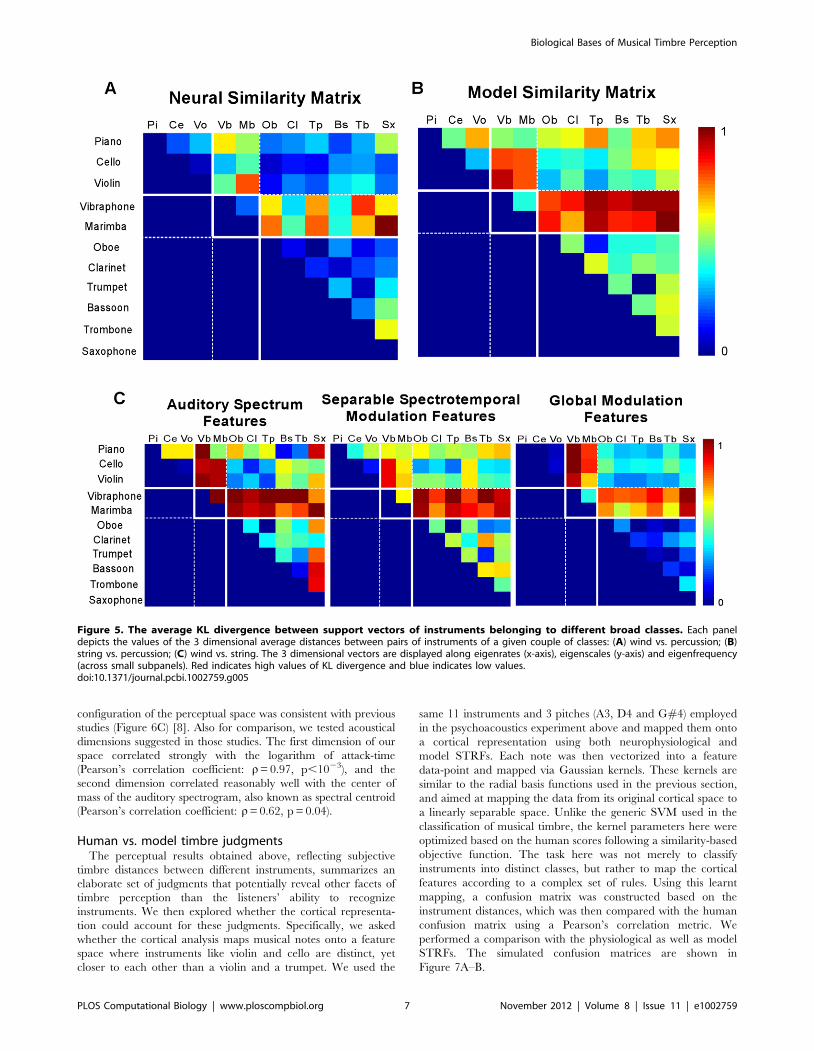
configuration of the perceptual space was consistent with previous
studies (Figure 6C) [8]. Also for comparison, we tested acoustical
dimensions suggested in those studies. The first dimension of our
space correlated strongly with the logarithm of attack-time
(Pearson’s correlation coefficient: r= 0.97, p,1023), and the
second dimension correlated reasonably well with the center of
mass of the auditory spectrogram, also known as spectral centroid
(Pearson’s correlation coefficient: r= 0.62, p = 0.04).
Human vs. model timbre judgmentsThe perceptual results obtained above, reflecting subjective
timbre distances between different instruments, summarizes an
elaborate set of judgments that potentially reveal other facets of
timbre perception than the listeners’ ability to recognize
instruments. We then explored whether the cortical representa-
tion could account for these judgments. Specifically, we asked
whether the cortical analysis maps musical notes onto a feature
space where instruments like violin and cello are distinct, yet
closer to each other than a violin and a trumpet. We used the
same 11 instruments and 3 pitches (A3, D4 and G#4) employed
in the psychoacoustics experiment above and mapped them onto
a cortical representation using both neurophysiological and
model STRFs. Each note was then vectorized into a feature
data-point and mapped via Gaussian kernels. These kernels are
similar to the radial basis functions used in the previous section,
and aimed at mapping the data from its original cortical space to
a linearly separable space. Unlike the generic SVM used in the
classification of musical timbre, the kernel parameters here were
optimized based on the human scores following a similarity-based
objective function. The task here was not merely to classify
instruments into distinct classes, but rather to map the cortical
features according to a complex set of rules. Using this learnt
mapping, a confusion matrix was constructed based on the
instrument distances, which was then compared with the human
confusion matrix using a Pearson’s correlation metric. We
performed a comparison with the physiological as well as model
STRFs. The simulated confusion matrices are shown in
Figure 7A–B.
Figure 5. The average KL divergence between support vectors of instruments belonging to different broad classes. Each paneldepicts the values of the 3 dimensional average distances between pairs of instruments of a given couple of classes: (A) wind vs. percussion; (B)string vs. percussion; (C) wind vs. string. The 3 dimensional vectors are displayed along eigenrates (x-axis), eigenscales (y-axis) and eigenfrequency(across small subpanels). Red indicates high values of KL divergence and blue indicates low values.doi:10.1371/journal.pcbi.1002759.g005
Biological Bases of Musical Timbre Perception
PLOS Computational Biology | www.ploscompbiol.org 7 November 2012 | Volume 8 | Issue 11 | e1002759
The success or otherwise of the different models was estimated
by correlating the human dissimilarity matrix to that generated by
the model. No attempt was made at producing MDS analyses of
the model output, as meaningfully comparing MDS spaces is not a
trivial problem [52]. Physiological STRFs yielded a correlation
coefficient of 0.73, while model STRFs yielded a correlation of
0.94 (Table 2).
Control experimentsIn order to disentangle the contribution of the ‘‘input’’ cortical
features versus the ‘‘back-end’’ machine learning in capturing
human behavioral data, we recomputed confusion matrices using
alternative representations such as the auditory spectrogram and
various marginals of the cortical distributions. In all these control
Figure 6. Human listener’s judgment of musical timbre similarity. (A) The mean (top row) and standard deviation (bottom row) of thelisteners’ responses show the similarity between every pair of instruments for three notes A3, D4 and G#4. Red (values close to 1) indicates highdissimilarity and blue (values close to 0) indicates similarity. (B) Timbre similarity is averaged across subjects, musical notes and upper and lower half-matrices, and used for validation of the physiological and computational model. (C) Multidimensional scaling (MDS) applied to the human similaritymatrix projected over 2 dimensions (shown to correlate with attack time and spectral centroid).doi:10.1371/journal.pcbi.1002759.g006
Biological Bases of Musical Timbre Perception
PLOS Computational Biology | www.ploscompbiol.org 8 November 2012 | Volume 8 | Issue 11 | e1002759
Biological Bases of Musical Timbre Perception
PLOS Computational Biology | www.ploscompbiol.org 9 November 2012 | Volume 8 | Issue 11 | e1002759
experiments, the Gaussian kernels were re-optimized separately to
fit the data representation being explored.
We first investigated the performance using auditory spectrum
features with optimized Gaussian kernels. The spectrogram
representation yielded a similarity matrix that captures the main
trends in human distance judgments, with a correlation coefficient
of 0.74 (Figure 7C, leftmost panel). Similar experiments using a
traditional spectrum (based on Fourier analysis of the signal) yield
a correlation of 0.69.
Next, we examined the effectiveness of the model cortical
features by reducing them to various marginal versions with fewer
dimensions as follows. First, we performed an analysis of the
spectral and temporal modulations as a separable cascade of two
operations. Specifically, we analyzed the spectral profile of the
auditory spectrogram (scales) independently from the temporal
dynamics (rates) and stack the two resulting feature vectors
together. This analysis differed from the full cortical analysis that
assumes an inseparable analysis of spectro-temporal features. An
inseparable function is one that cannot be factorized into a
function of time and a function of frequency; i.e. a matrix of rank
greater than 1 (see Methods). By construction, a separable function
consists of temporal cross sections that are scaled versions of the
same essential temporal function. A consequence of such
constraint is that a separable function cannot capture orientation
in time-frequency space (e.g. FM sweeps). In contrast, the full
cortical analysis estimates modulations along both time and
frequency axes in addition to an integrated view of the two axes
including orientation information The analysis based on the
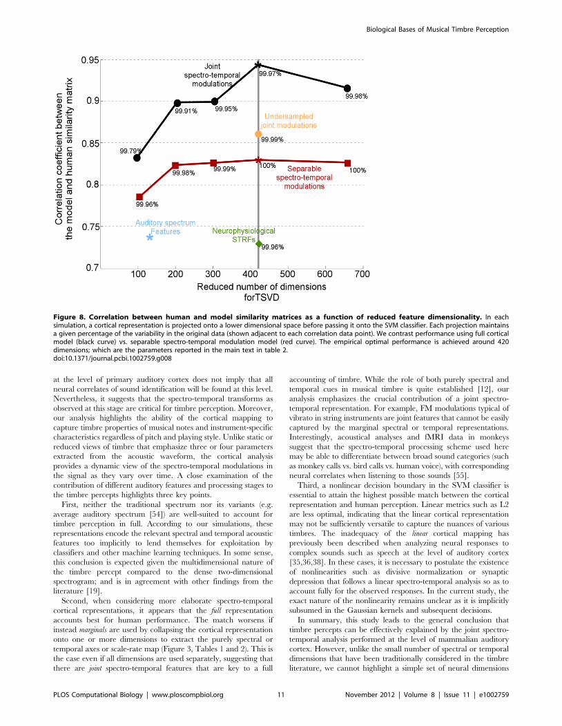
separable model achieved a correlation coefficient of 0.83(Table 2).
Second, we further reduced the separable spectro-temporal
space by analyzing the modulation content along both time and
frequency without maintaining the distribution along the tono-
topic axis. This was achieved by simply integrating the modulation
features along the spectral axis thus exploring the global
characteristic of modulation regardless of tonotopy (Figure 7C,
rightmost panel). This representation is somewhat akin to what
would result from a 2-dimensional Fourier analysis of the auditory
spectrogram. This experiment yielded a correlation coefficient of
0.70 (Table 2), supporting the value of an explicit tonotopic axis in
capturing subtle difference between instruments.
Next, we addressed the concern that the mere number of
features included in the full cortical model enough to explain the
observed performance. We therefore undersampled the full
cortical model by employing only 6 scale filters; 10 rate filters
and 64 frequency filters by coarsely sampling the range of spectro-
temporal modulations. This mapping resulted in a total number of
dimensions of 3840; to be comparable to the 4224 dimensions
obtained from the separable model. We then performed the
dimensionality reduction to 420 dimensions, similar to that used
for the separable analysis discussed above. The correlation
obtained was 0.86; which is better than that of the separable
spectro-temporal model (see Figure 8). This result supports our
main claim that the coverage provided by the cortical space allows
extracting specific details in the musical notes that highlight
information about the physical properties of each instrument;
hence enabling classification and recognition.
Finally, we examined the value of the kernel-learning compared
to using a simple Euclidian L2 distance at various stages of the
model (e.g. peripheral model, cortical stage, reduced cortical
model using tensor singular value decomposition). Table 2
summarizes the results of this analysis along various stages of the
model shown in Figure 2. The analysis revealed that the kernel-
based mapping does provide noticeable improvement to the
predictive power of the model but cannot –by itself– explain the
results since the same technique applied directly on the spectrum
only yielded a correlation of 0.74.
Discussion
This study demonstrates that perception of musical timbre could
be effectively based on neural activations patterns that sounds
evoke at the level of primary auditory cortex. Using neurophys-
iological recordings in mammalian auditory cortex as well as a
simplified model of cortical processing, it is possible to accurately
replicate human perceptual similarity judgments and classification
performance among sounds from a large number of musical
instruments. Of course, showing that the information is available
Figure 7. Model musical timbre similarity. Instrument similarity matrices based kernel optimization technique of the (A) neurophysiologicalreceptive field and (B) cortical model receptive fields. (C) Control experiments using the auditory spectral features (left), separable spectro-temporalmodulation feature (middle), and global modulation features [separable spectral and temporal modulations integrated across time and frequency](right). Red depicts high dissimilarity. All the matrices show only the upper half-matrix with the diagonal not shown.doi:10.1371/journal.pcbi.1002759.g007
Table 2. Correlation coefficients for different feature sets.
L2 on features L2 on reduced featuresGaussian kernels on reducedfeatures
Fourier-based Spectrum - - 0.69
Auditory Spectrum 0.473 - 0.739
Global Spectro-temporal Modulations 0.509 - 0.701
Separable Spectro-temporal Modulations 0.561 0.561 0.830
Full cortical Model 0.611 0.607 0.944
Neurophysiological STRFs - - 0.73
Each row represents the correlation coefficient between the model and human similarity matrix using a direct Euclidian distance the specific feature itself (left); on areduced dimension of the features (middle column) or using the Gaussian kernel distance (right column). Auditory Spectrum: time-average of the cochlear filterbank;Global Spectro-temporal Modulations: model STRFs averaged in time and frequency; Separable Spectro-temporal modulations: model STRFs averaged separately in rateand scale, and then in time; Full cortical model: STRFs averaged in time; Neurophysiological STRFs: as the full cortical model, but with STRFs collected in primaryauditory cortex of ferrets.doi:10.1371/journal.pcbi.1002759.t002
Biological Bases of Musical Timbre Perception
PLOS Computational Biology | www.ploscompbiol.org 10 November 2012 | Volume 8 | Issue 11 | e1002759
at the level of primary auditory cortex does not imply that all
neural correlates of sound identification will be found at this level.
Nevertheless, it suggests that the spectro-temporal transforms as
observed at this stage are critical for timbre perception. Moreover,
our analysis highlights the ability of the cortical mapping to
capture timbre properties of musical notes and instrument-specific
characteristics regardless of pitch and playing style. Unlike static or
reduced views of timbre that emphasize three or four parameters
extracted from the acoustic waveform, the cortical analysis
provides a dynamic view of the spectro-temporal modulations in
the signal as they vary over time. A close examination of the
contribution of different auditory features and processing stages to
the timbre percepts highlights three key points.
First, neither the traditional spectrum nor its variants (e.g.
average auditory spectrum [54]) are well-suited to account for
timbre perception in full. According to our simulations, these
representations encode the relevant spectral and temporal acoustic
features too implicitly to lend themselves for exploitation by
classifiers and other machine learning techniques. In some sense,
this conclusion is expected given the multidimensional nature of
the timbre percept compared to the dense two-dimensional
spectrogram; and is in agreement with other findings from the
literature [19].
Second, when considering more elaborate spectro-temporal
cortical representations, it appears that the full representation
accounts best for human performance. The match worsens if
instead marginals are used by collapsing the cortical representation
onto one or more dimensions to extract the purely spectral or
temporal axes or scale-rate map (Figure 3, Tables 1 and 2). This is
the case even if all dimensions are used separately, suggesting that
there are joint spectro-temporal features that are key to a full
accounting of timbre. While the role of both purely spectral and
temporal cues in musical timbre is quite established [12], our
analysis emphasizes the crucial contribution of a joint spectro-
temporal representation. For example, FM modulations typical of
vibrato in string instruments are joint features that cannot be easily
captured by the marginal spectral or temporal representations.
Interestingly, acoustical analyses and fMRI data in monkeys
suggest that the spectro-temporal processing scheme used here
may be able to differentiate between broad sound categories (such
as monkey calls vs. bird calls vs. human voice), with corresponding
neural correlates when listening to those sounds [55].
Third, a nonlinear decision boundary in the SVM classifier is
essential to attain the highest possible match between the cortical
representation and human perception. Linear metrics such as L2
are less optimal, indicating that the linear cortical representation
may not be sufficiently versatile to capture the nuances of various
timbres. The inadequacy of the linear cortical mapping has
previously been described when analyzing neural responses to
complex sounds such as speech at the level of auditory cortex
[35,36,38]. In these cases, it is necessary to postulate the existence
of nonlinearities such as divisive normalization or synaptic
depression that follows a linear spectro-temporal analysis so as to
account fully for the observed responses. In the current study, the
exact nature of the nonlinearity remains unclear as it is implicitly
subsumed in the Gaussian kernels and subsequent decisions.
In summary, this study leads to the general conclusion that
timbre percepts can be effectively explained by the joint spectro-
temporal analysis performed at the level of mammalian auditory
cortex. However, unlike the small number of spectral or temporal
dimensions that have been traditionally considered in the timbre
literature, we cannot highlight a simple set of neural dimensions
Figure 8. Correlation between human and model similarity matrices as a function of reduced feature dimensionality. In eachsimulation, a cortical representation is projected onto a lower dimensional space before passing it onto the SVM classifier. Each projection maintainsa given percentage of the variability in the original data (shown adjacent to each correlation data point). We contrast performance using full corticalmodel (black curve) vs. separable spectro-temporal modulation model (red curve). The empirical optimal performance is achieved around 420dimensions; which are the parameters reported in the main text in table 2.doi:10.1371/journal.pcbi.1002759.g008
Biological Bases of Musical Timbre Perception
PLOS Computational Biology | www.ploscompbiol.org 11 November 2012 | Volume 8 | Issue 11 | e1002759
subserving timbre perception. Instead, the model suggests that
subtle perceptual distinctions exhibited by human listeners are
based on ‘opportunistic’ acoustic dimensions [56] that are selected
and enhanced, when required, on the rich baseline provided by
the cortical spectro-temporal representation.
Methods
Ethics statementAll behavioral recordings of timbre similarity judgments with
human listeners were approved by the local ethics committee of
the Universite Paris Descartes. All procedures for recordings of
single unit neural activity in ferrets were in accordance with the
Institutional Animal Care and Use Committee at the University of
Maryland, College Park and the Guidelines of the National
Institutes of Health for use of animals in biomedical research.
PsychoacousticsStimuli. Recordings of single musical notes were extracted
from the RWC Music Database [57], using the notes designated
‘‘medium-volume’’ and ‘‘staccato’’, with pitches of A3, D4, and
G#4. The set used for the experiments comprised 13 sound
sources: Piano, Vibraphone, Marimba, Cello, Violin, Oboe,
Clarinet, Trumpet, Bassoon, Trombone, Saxophone, male singer
singing the vowel /a/, male singer singing the vowel /i/. Each
note was edited into a separate sound file, truncated to 250 ms
duration with 50 ms raised cosine offset ramp (the onset was
preserved), and normalized in RMS power. More details on the
sound set can be found in [56]. The analyses presented in the
current study exclude the results from the 2 vowels, as only musical
instruments were considered in the model classification experi-
ments.
Participants and apparatus. A total of twenty listeners
participated in the study (14 totally naıve participants, 6
participants experienced in psychoacoustics experiment but naıve
to the aim of the present study; mean age: 28 y; 10 female). They
had no self-reported history of hearing problems. All twenty
subjects performed the test with the D4 pitch. Only six took part in
the remaining tests with notes A3 and G#4. Results from the 6
subjects tested on all 3 notes are reported here, even though we
checked that including all subjects would not change our
conclusions. Stimuli were played through an RME Fireface
sound-card at a 16-bit resolution and a 44.1 kHz sample-rate.
They were presented to both ears simultaneously through
Sennheiser HD 250 Linear II headphones. Presentation level
was 65 dB(A). Listeners were tested individually in a double-walled
IAC sound booth.
Procedure. Subjective similarity ratings were collected. For a
given trial, two sounds were played with a 500 ms silent interval.
Participants had to indicate how similar they perceived the sounds
to be. Responses were collected by means of a graphical interface
with a continuous slider representing the perceptual similarity
scale. The starting position of the slider was randomized for each
trial. Participants could repeat the sound pair as often as needed
before recording their rating. In an experimental block, each
sound was compared to all others (with both orders of
presentations) but not with itself. This gave a total of 156 trials
per block, presented in random order. Before collecting the
experimental data, participants could hear the whole sound set
three times. A few practice trials were also provided until
participants reported having understood the task and instructions.
A single pitch was used for all instruments in each block; the three
types of blocks (pitch A3, D4, or G#4) were run in counterbal-
anced order across participants. Two blocks per pitch were run for
each participants, and only the second block was retained for the
analysis.Multidimensional scaling (MDS) and acoustical
correlates. To compare the results with previous studies, we
ran an MDS analysis on the dissimilarity matrix obtained from
human judgments. A standard non-metric MDS was performed
(Matlab, the MathWorks). Stress values were generally small, with
a knee-point for the solution at two dimensions (0.081, Kruskal
normalized stress1). We also computed acoustical descriptors
corresponding to the classic timbre dimensions. Attack time was
computed by taking the logarithm of the time taken to go from
240 dB to 212 dB relative to the maximum waveform amplitude.
Spectral centroid was computed by running the stimuli in an
auditory filterbank, compressing the energy in each channel
(exponent: 0.3), and taking the center of mass of the resulting
spectral distribution.
Auditory modelThe cortical model is comprised of two main stages: an early
stage mimicking peripheral processing up to the level of the
midbrain, and a central stage capturing processing in primary
auditory cortex (A1). Full details about the model can be found in
[54,58]; but are described briefly here.
The processing of the acoustic signal in the cochlea is modeled
as a bank of 128 constant-Q asymmetric bandpass filters equally
spaced on the logarithmic frequency scale spanning 5.3 octaves.
The cochlear output is then transduced into inner hair cells
potentials via a high pass and low pass operation. The resulting
auditory nerve signals undergo further spectral sharpening via a
lateral inhibitory network. Finally, a midbrain model resulting in
additional loss in phase locking is performed using short term
integration with time constant 4 ms resulting in a time frequency
representation called as the auditory spectrogram.
The central stage further analyzes the spectro-temporal content
of the auditory spectrogram using a bank of modulation selective
filters centered at each frequency along the tonotopic axis,
modeling neurophysiological receptive fields. This step corre-
sponds to a 2D affine wavelet transform, with a spectro-temporal
mother wavelet, define as Gabor-shaped in frequency and
exponential in time. Each filter is tuned (Q = 1) to a specific rate
(v in Hz) of temporal modulations and a specific scale of spectral
modulations (V in cycles/octave), and a directional orientation (+for upward and 2 for downward).
For input spectrogram z(t,f ), the response of each STRF in the
model is given by:
r+(t,f ; v,V; h,w)~z(t,f )�t,f STRF+(t,f ; v,V; h,w) ð1Þ
where �t,f denotes convolution in time and frequency and h and ware the characteristic phases of the STRF’s which determine the
degree of asymmetry in the time and frequency axes respectively.
The model filters STRFz(t,f ; v,V; h,w) filters can be decom-
posed in each quadrant (upward + or downward 2) into
RF(t; v; h) into SF(f ;V; w) corresponding to rate and scale filters
respectively. Details of the design of the filter functions STRFzcan be found in [58]. The present study uses 11 spectral filters with
characteristic scales [0.25, 0.35, 0.50, 0.71, 1.00, 1.41, 2.00, 2.83,
4.00, 5.66, 8.00] (cycles/octave) and 11 temporal filters with
characteristic rates [4.0, 5.7, 8.0, 11.3, 16.0, 22.6, 32.0, 45.3, 64.0,
90.5, 128.0] (Hz), each with upward and downward directionality.
All outputs are integrated over the time duration of each note. In
order to simplify the analysis, we limit our computations to the
magnitude of the cortical output rz(t,f ; v,V; h,w) (i.e. responses
corresponding to zero-phase filters).
Biological Bases of Musical Timbre Perception
PLOS Computational Biology | www.ploscompbiol.org 12 November 2012 | Volume 8 | Issue 11 | e1002759

Finally, dimensionality reduction is performed using tensor
singular-value decomposition [59]. This technique unfolds the
cortical tensor along each dimension (frequency, rate and scale
axes) and applies singular value decomposition on the unfolded
matrix. We choose 5 eigenscales, 4 eigenrates and 21 eigne-
frequencies resulting in 420 features with the highest eigenvalues,
preserving 99.9% of the variance in the original data. The
motivation for this cutoff choice is presented later.
Cortical receptive fieldsData used here was collected in the context of a number of
studies [60–62] and full details of the experimental paradigm are
described in these publications. Briefly, extracellular recordings
were performed in 15 awake non-behaving domestic ferrets
(Mustela putorius) with surgically implanted headposts. Tungsten
electrodes (3–8 MV) were used to record neural responses from
single and multi-units at different depths. All data was processed
off-line and sorted to extract single-unit activity.
Spectro-Temporal Receptive fields (STRF) were characterized
using TORC (Temporally-Orthogonal Ripple Combination)
stimuli [63], consisting of superimposed ripple noises with rates
between 4–24 (Hz) and scales between 0 (flat) and 1.4 peaks/
octave. Each stimulus was 3 sec with inter-stimulus intervals of 1–
1.2 sec, and a full set of 30 TORCs was typically repeated 6–15
times. All sounds were computer-generated and delivered to the
animal’s ear through inserted earphones calibrated in-situ. TORC
amplitude is fixed between 55–75 dB SPL.
STRFs were derived using standard reverse correlation
techniques, and a signal-to-noise ratio (SNR) for each STRF was
measured using a bootstrap technique (see [63] for details). Only
STRFs with SNR$2 were included in the current study, resulting
in a database of 1110 STRFs (average 74 STRFs/animal). Note
because of the experimental paradigm, STRFs spanned a 5-octave
range with low frequencies 125, 250 or 500 Hz. In the current
study, all STRFs were aligned to match the frequency range of
musical note spectrograms. Since all our spectrograms start at
180 Hz and cover 5.3 octaves, we scaled and shifted the STRF’s to
fit this range.
The neurophysiological STRFs were employed to perform the
timbre analysis by convolving each note’s auditory spectrogram
z(t,f) with each STRF in the database as in Equation (2).
rn(t,f )~z(t,f )�tSTRF (t,f ) ð2Þ
The resulting firing rate vector rn(t,f ) was then integrated over
time yielding an average response across the tonotopic axis. The
output from all STRFs were then stacked together, resulting in a
142080 (128 frequency channels 61110 STRFs) dimensional
vector. We reduced this vector using singular value decomposition
and mapped it onto 420 dimensions, which preserve 99.9% of the
data variance in agreement with dimensionality used for model
STRFs.
Timbre classificationIn order to test the cortical representation’s ability to
discriminate between different musical instruments, we augmented
the basic auditory model with a statistical clustering model based
on support vector machines (SVM) [39]. Support vector machines
are classifiers that learn a set of hyperplanes (or decision
boundaries) in order to maximally separate the patterns of cortical
responses caused by the different instruments.
Each cortical pattern was projected via Gaussian kernel to a
new dimensional space. The use of kernels is a standard technique
used with support vector machines, aiming to map the data from
its original space (where data may not be linearly separable) onto a
new representational space that is linearly separable. This
mapping of data to a new (more linear space) through a the use
of a kernel or transform is commonly referred to as the ‘‘kernel
trick’’ [39]. In essence, kernel functions aim to determine the
relative position or similarity between pairs of points in the data.
Because the data may lie in a space that is not linearly separable
(not possible to use simple lines or planes to separate the different
classes), it is desirable to map the data points onto a different space
where this linear separability is possible. However, instead of
simply projecting the data points themselves onto a high-
dimensional feature space which would increase complexity as a
function of dimensionality, the ‘‘kernel trick’’ avoids this direct
mapping. Instead, it provides a method for mapping the data into
an inner product space without explicitly computing the mapping
of the observations directly. In other words, it computes the inner
product between the data points in the new space without
computing the mapping explicitly.
The kernel used here is given by
K(x,y)~e{
x{yð ÞT x{yð Þs
� �ð3Þ
where x and y are the feature vectors of 2 sound samples. The
parameter for the Gaussian kernel and the cost parameter for the
SVM algorithm were optimized on a subset of the training data.
A classifier Cij is trained for every pair of classes i and j. Each of
these classifiers then gives a label lij for a test sample. Note that
lij~i or j. We count the number of labels Ri~P
1(lij~i). The
test sample is then assigned to the class with maximum count given
by arg maxiRi. The parameter s in Equation (3) was chosen by
doing a grid search over a large parameter span in order to
optimize the classifier performance in correctly distinguishing
different instruments. This tuning was done by training and testing
on a subset of the training data. For model testing, we performed a
standard k-fold cross validation procedure with k = 10 (90%
training, 10% testing). The dataset was divided into 10 parts. We
then left out one part at a time and trained on the remaining 9
parts. The results reported are the average performance over all 10
iterations. A single Gaussian parameter was optimized for all the
pair-wise classifiers across all the 10-fold cross validation
experiments.
Analysis of support vector distributionIn order to better understand the mapping of the different notes
in the high-dimensional space used to classify them, we performed
a closer analysis of the support vectors for each instrument pair i
and j. Support vectors are the samples from each class that fall
exactly on the margin between class i and class j, and therefore are
likely to be more confusable between the classes. Since we are
operating in the ‘classifier space’, each of the support vectors is
defined in a reduced dimensional hyperspace consisting of 5 eigen-
scales, 4 eigen-rates, and 21 eigen-frequencies as explained above
(a total of 420 dimensions). The collection of all support vectors for
each class i can be pulled together to estimate a high-dimensional
probability density function. The density function estimate was
derived using a histogram method by partitioning the sample
space along each dimension into 100 bins, counting how many
samples fall into each bin and dividing the counts by the total
number of samples. We label the probability distribution for the d-
th dimension (d = 1,..,420) pi,d . We then computed the symmetric
KL divergence, KLi,j(d) [43], between the support vectors for
classes i and j from the classifier Ci,j as shown in Equation (4). The
Biological Bases of Musical Timbre Perception
PLOS Computational Biology | www.ploscompbiol.org 13 November 2012 | Volume 8 | Issue 11 | e1002759
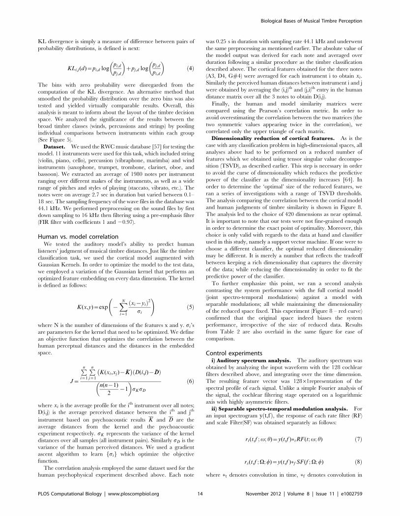
KL divergence is simply a measure of difference between pairs of
probability distributions, is defined is next:
KLi,j(d)~pi,d logpi,d
pj,d
� �zpj,d log
pj,d
pi,d
� �ð4Þ
The bins with zero probability were disregarded from the
computation of the KL divergence. An alternative method that
smoothed the probability distribution over the zero bins was also
tested and yielded virtually comparable results. Overall, this
analysis is meant to inform about the layout of the timbre decision
space. We analyzed the significance of the results between the
broad timbre classes (winds, percussions and strings) by pooling
individual comparisons between instruments within each group
(See Figure 5).
Dataset. We used the RWC music database [57] for testing the
model. 11 instruments were used for this task, which included string
(violin, piano, cello), percussion (vibraphone, marimba) and wind
instruments (saxophone, trumpet, trombone, clarinet, oboe, and
bassoon). We extracted an average of 1980 notes per instrument
ranging over different makes of the instruments, as well as a wide
range of pitches and styles of playing (staccato, vibrato, etc.). The
notes were on average 2.7 sec in duration but varied between 0.1–
18 sec. The sampling frequency of the wave files in the database was
44.1 kHz. We performed preprocessing on the sound files by first
down sampling to 16 kHz then filtering using a pre-emphasis filter
(FIR filter with coefficients 1 and 20.97).
Human vs. model correlationWe tested the auditory model’s ability to predict human
listeners’ judgment of musical timbre distances. Just like the timbre
classification task, we used the cortical model augmented with
Gaussian Kernels. In order to optimize the model to the test data,
we employed a variation of the Gaussian kernel that performs an
optimized feature embedding on every data dimension. The kernel
is defined as follows:
K(x,y)~exp {XN
i~1
xi{yið Þ2
si
!ð5Þ
where N is the number of dimensions of the features x and y. si’s
are parameters for the kernel that need to be optimized. We define
an objective function that optimizes the correlation between the
human perceptual distances and the distances in the embedded
space.
J~
Pni~1
Pnj~1
K(xi,xj){ �KK� �
D(i,j){�DDð Þ
n(n{1)
2{1
� �sK sD
ð6Þ
where xi is the average profile for the ith instrument over all notes;
D(i,j) is the average perceived distance between the ith and jth
instrument based on psychoacoustic results K and D are the
average distances from the kernel and the psychoacoustic
experiment respectively. sK represents the variance of the kernel
distances over all samples (all instrument pairs). Similarly sD is the
variance of the human perceived distances. We used a gradient
ascent algorithm to learn fsig which optimize the objective
function.
The correlation analysis employed the same dataset used for the
human psychophysical experiment described above. Each note
was 0.25 s in duration with sampling rate 44.1 kHz and underwent
the same preprocessing as mentioned earlier. The absolute value of
the model output was derived for each note and averaged over
duration following a similar procedure as the timbre classification
described above. The cortical features obtained for the three notes
(A3, D4, G#4) were averaged for each instrument i to obtain xi.
Similarly the perceived human distances between instrument i and j
were obtained by averaging the (i,j)th and (j,i)th entry in the human
distance matrix over all the 3 notes to obtain D(i,j).
Finally, the human and model similarity matrices were
compared using the Pearson’s correlation metric. In order to
avoid overestimating the correlation between the two matrices (the
two symmetric values appearing twice in the correlation), we
correlated only the upper triangle of each matrix.
Dimensionality reduction of cortical features. As is the
case with any classification problem in high-dimensional spaces, all
analyses above had to be performed on a reduced number of
features which we obtained using tensor singular value decompo-
sition (TSVD), as described earlier. This step is necessary in order
to avoid the curse of dimensionality which reduces the predictive
power of the classifier as the dimensionality increases [64]. In
order to determine the ‘optimal’ size of the reduced features, we
ran a series of investigations with a range of TSVD thresholds.
The analysis comparing the correlation between the cortical model
and human judgments of timbre similarity is shown in Figure 8.
The analysis led to the choice of 420 dimensions as near optimal.
It is important to note that our tests were not fine-grained enough
in order to determine the exact point of optimality. Moreover, this
choice is only valid with regards to the data at hand and classifier
used in this study, namely a support vector machine. If one were to
choose a different classifier, the optimal reduced dimensionality
may be different. It is merely a number that reflects the tradeoff
between keeping a rich dimensionality that captures the diversity
of the data; while reducing the dimensionality in order to fit the
predictive power of the classifier.
To further emphasize this point, we ran a second analysis
contrasting the system performance with the full cortical model
(joint spectro-temporal modulations) against a model with
separable modulations; all while maintaining the dimensionality
of the reduced space fixed. This experiment (Figure 8 – red curve)
confirmed that the original space indeed biases the system
performance, irrespective of the size of reduced data. Results
from Table 2 are also overlaid in the same figure for ease of
comparison.
Control experimentsi) Auditory spectrum analysis. The auditory spectrum was
obtained by analyzing the input waveform with the 128 cochlear
filters described above, and integrating over the time dimension.
The resulting feature vector was 12861representation of the
spectral profile of each signal. Unlike a simple Fourier analysis of
the signal, the cochlear filtering stage operated on a logarithmic
axis with highly asymmetric filters.
ii) Separable spectro-temporal modulation analysis. For
an input spectrogram y t,fð Þ, the response of each rate filter (RF)
and scale Filter(SF) was obtained separately as follows:
rt(t,f ; v; h)~y(t,f )�tRF (t; v; h) ð7Þ
rs(t,f ;V; w)~y(t,f )�f SF (f ;V; w) ð8Þ
where �t denotes convolution in time, �f denotes convolution in
Biological Bases of Musical Timbre Perception
PLOS Computational Biology | www.ploscompbiol.org 14 November 2012 | Volume 8 | Issue 11 | e1002759
frequency and h is the characteristic phase of the RF and w is the
characteristic phase of the SF which determine the degree of
asymmetry in the time and frequency axis respectively. Details of
the design of the filter functions SF and RF can be found in [58].
Unlike the analysis given in Equation (1), the spectral and
temporal modulations were derived separately using one-dimen-
sional complex-valued filters (either along time or along frequency
axis). The resulting magnitude outputs from Equations (7–8) were
then stacked together to form the feature vector with 4224
(11scales6128frequecies+22rates6128frequecies) dimensions. The
dimensionality was then reduced to 420 using tensor singular value
decomposition retaining 99.9% of the variance.iii) Global modulation analysis. For this experiment, we
used the rt(t,f ; v; h) and rs(t,f ;V; w) from Equations (7–8), and
integrated the output over time and frequency for each note. The
resulting rate and scale responses were then stacked together to
form the feature vector.iv) Under sampled joint modulation. In this experiment
we aimed to make the dimensionality of the cortical model
comparable to the separable model by under sampling the rate,
scale and frequency axes. The auditory spectrogram was down
sampled along the frequency axis by a factor of 2. This auditory
spectrogram representation was then analyzed by 6 spectral filters
with characteristic scales [0.25, 0.47, 0.87, 1.62, 3.03, 5.67]
(cycles/octave) and 5 temporal filters with characteristic rates [4.0,
8.0, 16.0, 32.0, 64.0] (Hz), each with upward and downward
directionality resulting in a 3840 dimensional representation. The
dimensionality was then reduced to 420 using tensor singular value
decomposition retaining 99.99% of the variance
Author Contributions
Conceived and designed the experiments: KP DP SS ME. Performed the
experiments: KP DP SS ME. Analyzed the data: KP DP SS ME.
Contributed reagents/materials/analysis tools: KP DP SS ME. Wrote the
paper: KP DP SS ME.
References
1. Handel S (1993) Listening: An introduction to the perception of auditory events.
Cambridge, MA: MIT Press.
2. Ansi PT (1973) Psychoacoustical Terminology. New York: American National
Standards Institute.
3. Helmholtz H (1877) On the Sensations of Tone. New York: Dover Publications.
4. Grey JM, Gordon JW (1978) Perceptual effects of spectral modifications onmusical timbres. J Acoust Soc Am 63: 1493–1500.
5. McAdams S, Beauchamp JW, Meneguzzi S (1999) Discrimination of musical
instrument sounds resynthesized with simplified spectrotemporal parameters.J Acoust Soc Am 105: 882–897.
6. Patterson RD (1994) The sound of a sinusoid: Time-interval models. J Acoust
Soc Am 96: 1419–1428.
7. krumhansl C (1989) Why is musical timbre so hard to understand? In: Olsson
SNaO, editor. structure and perception of electroacoustic sound and music.
Amsterdam: Excerpta medica. pp. 43–53.
8. McAdams S, Winsberg S, Donnadieu S, De Soete G, Krimphoff J (1995)
Perceptual scaling of synthesized musical timbres: common dimensions,
specificities, and latent subject classes. Psychol Res 58: 177–192.
9. Grey JM (1977) Multidimensional perceptual scaling of musical timbres. J Acoust
Soc Am 61: 1270–1277.
10. J A Burgoyne SM (2007) A Meta-analysis of Timbre Perception Using NonlinearExtensions to CLASCAL. In: Proceedings of the Computer Music Modeling and
Retrieval. Copenhagen, Denmark. pp. 181–202.
11. Donnadieu S (2007) Mental Representation of the Timbre of Complex Sounds.In: Beauchamp J, editor. Analysis, Synthesis, and Perception of Musical Sounds.
New York: Springer. pp. 272–319.
12. Peeters G, Giordano BL, Susini P, Misdariis N, McAdams S (2011) The TimbreToolbox: extracting audio descriptors from musical signals. J Acoust Soc Am
130: 2902–2916.
13. Caclin A, McAdams S, Smith BK, Winsberg S (2005) Acoustic correlates oftimbre space dimensions: a confirmatory study using synthetic tones. J Acoust
Soc Am 118: 471–482.
14. Waibel A, Lee K (1990) Readings in speech recognition: Morgan KaufmannPub. Inc. 680 p.
15. Eidenberger H (2011) Fundamental Media Understanding. Norderstedt,
Germany: atpress.
16. Rabiner L, Juang B (1993) Fundamentals of Speech Recognition. New Jersey,USA: PTR Prentice Hall.
17. McKinney M, Breebaart J (2003) Features for Audio and Music Classification.
In: Proceedings of International Symposium on Music Information Retrieval.Washington D.C, USA. pp. 151–158.
18. Lerch A (2012) An Introduction to Audio Content Analysis: Applications in
Signal Processing and Music Informatics. New Jersey, USA: Wiley-IEEE Press.
19. Herrera-Boyer P, Peeters G, Dubnov S (2003) Automatic classification of
musical instrument sounds. Journal of New Music Research 32: 3–21.
20. Burred JJ, Haller M, Jin S, Samour A, Sikora T (2008) Audio Content Analysis.In: Kompatsiaris Y, Hobson P, editors. Semantic Multimedia and Ontologies:
Theory and Applications. London, UK: Springer. pp. 123–162.
21. Caclin A, Brattico E, Tervaniemi M, Naatanen R, Morlet D, et al. (2006)Separate neural processing of timbre dimensions in auditory sensory memory.
J Cogn Neurosci 18: 1959–1972.
22. Belin P, Zatorre RJ, Lafaille P, Ahad P, Pike B (2000) Voice-selective areas inhuman auditory cortex. Nature 403: 309–312.
23. Uppenkamp S, Johnsrude IS, Norris D, Marslen-Wilson W, Patterson RD
(2006) Locating the initial stages of speech-sound processing in human temporalcortex. NeuroImage 31: 1284–1296.
24. Lewis JW, Brefczynski JA, Phinney RE, Janik JJ, DeYoe EA (2005) Distinct
cortical pathways for processing tool versus animal sounds. J Neurosci 25: 5148–5158.
25. Leaver AM, Rauschecker JP (2010) Cortical representation of natural complex
sounds: effects of acoustic features and auditory object category. J Neurosci 30:7604–7612.
26. De Lucia M, Clarke S, Murray MM (2010) A temporal hierarchy for conspecific
vocalization discrimination in humans. J Neurosci 30: 11210–11221.
27. Staeren N, Renvall H, De Martino F, Goebel R, Formisano E (2009) Sound
categories are represented as distributed patterns in the human auditory cortex.Curr Biol 19: 498–502.
28. Formisano E, De Martino F, Bonte M, Goebel R (2008) ‘‘Who’’ is saying
‘‘what’’? Brain-based decoding of human voice and speech. Science 322: 970–973.
29. Miller LM, Escabi MA, Read HL, Schreiner CE (2002) Spectrotemporal
receptive fields in the lemniscal auditory thalamus and cortex. J Neurophysiol
87: 516–527.
30. Atencio CA, Schreiner CE (2010) Laminar diversity of dynamic soundprocessing in cat primary auditory cortex. J Neurophysiol 103: 192–205.
31. Schreiner CE, Sutter ML (1992) Topography of excitatory bandwidth in cat
primary auditory cortex: single-neuron versus multiple-neuron recordings.J Neurophysiol 68: 1487–1502.
32. Versnel H, Shamma S, Kowalski N (1995) Ripple Analysis in the Ferret Primary
Auditory Cortex. III. Topographic and Columnar Distribution of Ripple
Response. Auditory Neuroscience: 271–285.
33. Schreiner CE, Mendelson J, Raggio MW, Brosch M, Krueger K (1997)Temporal processing in cat primary auditory cortex. Acta Otolaryngol Suppl
532: 54–60.
34. Theunissen FE, Sen K, Doupe AJ (2000) Spectral-temporal receptive fields ofnonlinear auditory neurons obtained using natural sounds. J Neurosci 20: 2315–
2331.
35. Elhilali M, Fritz JB, Klein DJ, Simon JZ, Shamma SA (2004) Dynamics of
precise spike timing in primary auditory cortex. J Neurosci 24: 1159–1172.
36. Christianson GB, Sahani M, Linden JF (2008) The consequences of responsenonlinearities for interpretation of spectrotemporal receptive fields. J Neurosci
28: 446–455.
37. David SV, Mesgarani N, Fritz JB, Shamma SA (2009) Rapid synaptic depressionexplains nonlinear modulation of spectro-temporal tuning in primary auditory
cortex by natural stimuli. J Neurosci 29: 3374–3386.
38. Sadagopan S, Wang X (2009) Nonlinear spectrotemporal interactions
underlying selectivity for complex sounds in auditory cortex. J Neurosci 29:11192–11202.
39. Cristianini N, Shawe-Taylor J (2000) Introduction to support vector machines
and other kernel-based learning methods. Cambridge, UK: CambridgeUniversity Press.
40. Elhilali M, Fritz JB, Chi TS, Shamma SA (2007) Auditory cortical receptive
fields: stable entities with plastic abilities. Journal of Neuroscience 27: 10372–
10382.
41. Livshin A, X.Rodet (2004) Musical instrument identification in continuousrecordings. In: Proceedings of 7th International Conference on Digital Audio
Effects. Naples, Italy. pp. 222–227.
42. Burred JJ, Robel A, Sikora T (2010) Dynamic Spectral Envelope Modeling forTimbre Analysis of Musical Instrument Sounds. Ieee Transactions on Audio
Speech and Language Processing 18: 663–674.
43. Cover T, Thomas J (2006) Elements of information theory. New York: Wiley-
Interscience.
Biological Bases of Musical Timbre Perception
PLOS Computational Biology | www.ploscompbiol.org 15 November 2012 | Volume 8 | Issue 11 | e1002759
44. Krishna AG, Sreenivas TV (2004) Music instrument recognition: from isolated
notes to solo phrases. In: Proceedings of IEEE International Conference onAcoustics, Speech, and Signal Processing. Montreal,Quebec,Canada. pp. iv265–
iv268.
45. Marques J, Moreno PJ (1999) A study of musical instrument classification usingGaussian Mixture Models and Support Vector Machines. Compaq Corporation,
Cambridge Research laboratory.46. Brown JC, Houix O, McAdams S (2001) Feature dependence in the automatic
identification of musical woodwind instruments. J Acoust Soc Am 109: 1064–
1072.47. Kitahara T, Goto M, Okuno HG (2003) Musical instrument identification based
on f0-dependent multivariate normal distribution. In: Proceedings of IEEEInternational Conference on Acoustics, Speech and Signal Processing. Hong
Kong. pp. 409–412.48. Eronen A, Klapuri A (2000) Musical instrument recognition using cepstral
coefficients and temporal features. In: Proceedings of IEEE International
Conference on Acoustics, Speech, and Signal Processing. Istanbul, Turkey. pp.II753–II756.
49. Agostini G, Longari M, Pollastri E (2001) Musical instrument timbresclassification with spectral features. In: Proceedings of IEEE Fourth Workshop
on Multimedia Signal Processing. Cannes, France. pp. 97–102.
50. Livshin A, Rodet X (2006) The Significance of the Non-Harmonic ‘‘Noise’’Versus the Harmonic Series for Musical Instrument Recognition. In:
Proceedings of the 7th International Conference on Music InformationRetrieval. Victoria, Canada pp. 95–100.
51. Kostek B (2004) Musical instrument classification and duet analysis employingmusic information retrieval techniques. Proceedings of the IEEE 92: 712–729.
52. Marozeau J, de Cheveigne A, McAdams S, Winsberg S (2003) The dependency
of timbre on fundamental frequency. J Acoust Soc Am 114: 2946–2957.53. Cox TF, Cox MAA (2001) Multidimensional Scaling. London, UK: Chapman
and Hall.
54. Yang X, Wang K, Shamma SA (1992) Auditory representations of acoustic
signals. IEEE Trans Inf Theory 38: 824–839.
55. Joly O, Ramus F, Pressnitzer D, Vanduffel W, Orban GA (2012) Interhemi-
spheric Differences in Auditory Processing Revealed by fMRI in Awake Rhesus
Monkeys. Cereb Cortex 22: 838–853.
56. Agus TR, Suied C, Thorpe SJ, Pressnitzer D (2012) Fast recognition of musical
sounds based on timbre. J Acoust Soc Am 131: 4124–4133.
57. Goto M, Hashiguchi H, Nishimura T, Oka R (2003) RWC music database:
Music genre database and musical instrument sound database. In: Proceedings
of International Symposium on Music Information Retrieval. Washington D.C,
USA. pp. 229–230.
58. Chi T, Ru P, Shamma SA (2005) Multiresolution spectrotemporal analysis of
complex sounds. J Acoust Soc Am 118: 887–906.
59. De Lathauwer L, De Moor B, Vandewalle J (2000) A multilinear singular value
decomposition. SIAM Journal on Matrix Analysis and Applications 21: 1253–
1278.
60. Fritz J, Shamma S, Elhilali M, Klein D (2003) Rapid task-related plasticity of
spectrotemporal receptive fields in primary auditory cortex. Nat Neurosci 6:
1216–1223.
61. Fritz JB, Elhilali M, Shamma SA (2005) Differential dynamic plasticity of A1
receptive fields during multiple spectral tasks. J Neurosci 25: 7623–7635.
62. Fritz JB, Elhilali M, Shamma SA (2007) Adaptive changes in cortical receptive
fields induced by attention to complex sounds. Journal of Neurophysiology 98:
2337–2346.
63. Klein DJ, Depireux DA, Simon JZ, Shamma SA (2000) Robust spectrotemporal
reverse correlation for the auditory system: optimizing stimulus design. J Comput
Neurosci 9: 85–111.
64. Donoho D (2000) High-Dimensional Data Analysis : The Curses and Blessings
of Dimensionality. Aide-Memoire of a Lecture at AMS Conference on Math
Challenges of the 21st Century. Los Angeles, California, USA.
Biological Bases of Musical Timbre Perception
PLOS Computational Biology | www.ploscompbiol.org 16 November 2012 | Volume 8 | Issue 11 | e1002759