To appear in the ACM SIGGRAPH conference proceedings

Musculotendon Simulation for Hand Animation

Shinjiro Sueda Andrew Kaufman Dinesh K. Pai

Sensorimotor Systems LaboratoryUniversity of British Columbia∗

Modeling Animation Activation, Simulation Basic Skinning Final Output

Figure 1: Pipeline: The user specifies the model and its corresponding animation. Our system computes the required activations, andsimulates the muscles, tendons, and bones. The skin is then attached to the skeleton, and the subcutaneous deformation from tendon motionis added as a post-process.

Abstract

We describe an automatic technique for generating the motion oftendons and muscles under the skin of a traditionally animatedcharacter. This is achieved by integrating the traditional animationpipeline with a novel biomechanical simulator capable of dynamicsimulation with complex routing constraints on muscles and ten-dons. We also describe an algorithm for computing the activationlevels of muscles required to track the input animation. We demon-strate the results with several animations of the human hand.

CR Categories: I.3.7 [Computer Graphics]: Three-DimensionalGraphics and Realism—Animation I.6.8 [Simulation and Model-ing]: Types of Simulation—Animation

Keywords: musculoskeletal simulation, character animation, sec-ondary motion

1 Introduction

Human bodies are more than skin and bones. When the bodymoves, tendons and muscles move under the skin in visually im-portant ways that are correlated with both the movement and the in-ternal forces. For example, the appearance of tendons on the backof the hand is related to how the hand is moving and how muchforce it is exerting. Even though there has been some work on in-corporating muscles into animations (see Sec. 2 for a review) it hasbeen very difficult to incorporate biomechanically realistic subcuta-neous movements into a traditional animation pipeline. Integration

∗e-mail:{sueda, akaufman, pai}@cs.ubc.ca

with a traditional character animation pipeline is important since,unlike secondary motion of inanimate objects, the movements ofcharacters are of central importance to the story and are typicallyhand crafted by expert animators.

In this paper we describe an automatic technique for generatingbiomechanically realistic secondary motion that fits into a tradi-tional animation pipeline. In our system, animators are given arigged character, and animate it as they normally would, for in-stance, using key frame techniques or motion capture. The anima-tion is then exported to our efficient biomechanics simulator, basedon Lagrangian dynamics. We constrain the animated bones to fol-low the animator’s chosen motion path. We perform an optimiza-tion to determine the appropriate activation levels for each musclethroughout the animation. We then export the resulting physicallybased animations of musculotendons from our simulator and importthem back into the rigged animation scene. The tendons are auto-matically skinned to the character’s surface skin, providing com-plex secondary motion of the skin as a result of biomechanicallyrealistic tendon motion.

Our method works well with areas where muscles and tendons arenear the surface with little subcutaneous fat. We show the effective-ness of the method by simulating the musculotendons of the humanhand and forearm.

Our main contributions are:

• A novel, efficient biomechanical simulator that can simulatethin strands including tendons and muscles, with complexrouting constraints.

• Seamless integration of biomechanically realistic secondaryanimation into a traditional animation pipeline.

• An incremental algorithmic controller that determines themuscle activation levels required to dynamically track a tar-get animation.

2 Related Work

We will first review several common muscle models used in boththe computer graphics and biomechanics communities; we alsobriefly cover work related to strand simulation. Then we will dis-cuss various methods for musculoskeletal control.

1

To appear in the ACM SIGGRAPH conference proceedings

2.1 Muscle Simulation

Much of the work in musculoskeletal models has its roots in thebiomechanics community [Delp and Loan 1995; Hogfors et al.1995; Delp and Loan 2000; Pandy 2001; Maural et al. 1996; Chao2003; Blemker and Delp 2005; Rasmussen et al. 2005; Wu et al.2007]. With a few exceptions, muscles are modeled by simple linesof force that can bend around kinematic wrapping surfaces. Nonehave been able to represent the complex tendon routing constraintsthat we demonstrate in this paper.

There has also been significant development of musculoskeletalmodels in the graphics community. Some have focused only on themuscle anatomy, and not on dynamic simulation [Scheepers et al.1997; Wilhelms and Gelder 1997; Albrecht et al. 2003]. Ng-Thow-Hing [2001] and Teran et al. [2003; 2005] developed volumetricmuscle models to simulate muscles with both active and passivecomponents. Zhu et al. [1998] use a linear elastic muscle modelalong with finite elements for muscle volume deformation. Mauralet al. [1996] and Aubel and Thalmann [2001] constructed muscle-based virtual human characters. Musculoskeletal models have alsobeen used extensively for facial animation [Waters 1987; Lee et al.1995; Sifakis et al. 2005]. Shao and Ng-Thow-Hing [2003] pre-sented a general joint component framework designed to improvethe realism of joint articulation in virtual humans. Lee and Ter-zopoulos [2006] used a neuromuscular control model for the sim-ulation of a human neck. Zordan et al. [2004] developed muscleelements based on springs for simulated respiration.

Our muscle-tendon model relies on simulating thin structures wecall strands. There have been several papers in the graphics litera-ture investigating the use of thin physical structures for simulationof various phenomena [Qin and Terzopoulos 1996; Remion et al.1999; Pai 2002; Grinspun et al. 2003; Lenoir et al. 2004; Cole-man and Singh 2006; Bertails et al. 2006; Spillmann and Teschner2007]. Our model extends these with new constraints and activa-tion.

2.2 Muscle Control

There has been significant work in developing algorithmic con-trollers for physically based animation, without taking muscles intoaccount [Faloutsos et al. 2001; Pollard and Zordan 2005]. Somecontrollers are able to achieve high realism by incorporating mo-tion and force capture data [Yin et al. 2003; Zordan et al. 2005; Kryand Pai 2006].

Among the papers that take muscles explicitly into account andsolve for their control signals, many use joint moment-arms, whichare commonly used biomechanical approximation of distributedmuscle forces around joints [Thelen et al. 2002; Tsang et al. 2005;Thelen and Anderson 2006]. Sifakis et al. [2005] determine activa-tions of a detailed non-linear, but quasistatic, FEM muscle model.Weinstein et al. [2008] use a novel approach to PD control of mus-cles to track an animation. Lee and Terzopoulos [2006] use neuralnetworks to learn to control the complex musculature of the neck.

3 Strand Based Musculoskeletal Simulation

Our simulator is built on two primitives: rigid bodies for bonesand spline-based strands for tendons and muscles. Our decisionto use strands was motivated by the anatomical structure of realmuscle tissue. Muscles consist of fibers, curved in space, which arebundled into groups called fascicles. When a muscle is activated,the fibers contract, which transmits a contractile force directly alongeach fiber. By using strands in our muscle simulation, we are ableto directly model this behavior. Strands allow us to define smooth

curves to represent tendons, muscles, or the individual fascicles ofeach muscle. The forces applied to the strands can be transmitteddirectly along the curve, and also laterally through constraints.

We extend the physically-based spline models previously used incomputer graphics [Qin and Terzopoulos 1996; Remion et al. 1999;Lenoir et al. 2004] to include activation (Sec. 3.2), simple yet ro-bust sliding and surface constraint models (Sec. 3.3), and implicitintegration with Rayleigh damping (Sec. 3.4).

A strand, containing n ≥ 4 control points, has 3n degrees of free-dom, corresponding to the x, y, and z coordinates of the n controlpoints. The state of the system is given by the stacked positionsand velocities of the rigid bodies and strand control points. Theseare the generalized coordinates and velocities of the system, respec-tively:

χ =[· · · Ei · · · qj · · ·

]TΦ =

[· · · φi · · · qj · · ·

]T.

(1)

Here, Ei ∈ SE(3) and φi ∈ se(3) are the configuration and thespatial velocity, respectively, of the ith rigid body (SE(3) is thespace of 3D positions and orientations, and se(3) is the space oftranslational and rotational velocities), and qj ∈ R3 and qj ∈ R3

are the position and the velocity of the jth spline control point.

For each generalized coordinate, we construct an impulse-momentum equation which, when discretized at the velocity level,is

MΦ(k+1) = MΦ(k) + hf −GTλ, (2)

where M is the block-diagonal generalized mass matrix of rigidbodies and strand control points [Remion et al. 1999], h is the stepsize, f is the generalized force (body forces for rigid bodies, elasticand damping forces for strands, etc., Sec. 3.2), and GTλ is theconstraint force (Sec. 3.3).

3.1 Rigid Bodies and Joints

We can treat bones as rigid, since their deformation is not importantfor our purposes. The world position and velocity of a point on arigid body at a local coordinate r are given by

x = E r

x = E−T Γ(r)φ,(3)

where E is the usual coordinate transformation matrix and the 3×6matrix, Γ = (−[r] I), transforms the local spatial velocity of therigid body, φ, into the velocity of a local point, r, on the rigid bodyin local coordinates. The 3 × 3 matrix, [r], is the cross-productmatrix such that [r]v = r × v. Joint constraints are implementedusing the adjoint formulation [Murray et al. 1994], with which wecan easily derive different types of joints by simply dropping rowsin the 6 × 6 adjoint matrix. For example, we drop the top threerows (corresponding to the three rotational DoFs) for a ball joint, orthe third row (corresponding to the rotation about the z-axis) for ahinge joint.

3.2 Strand Dynamics

The path of a strand is described by a cubic B-spline curve,

p(s, t) =

3∑i=0

bi(s)qi(t), (4)

where qi(t) denote the control points of the strand, with velocitiesqi(t). The cubic B-spline basis functions, bi(s), depend on where

2

To appear in the ACM SIGGRAPH conference proceedings

the point is along the spline. Although a strand can have an arbitrarynumber of control points, a point on a strand only depends on fourcontrol points, due to the local support of the B-spline basis. Thevelocity and the tangent vectors of a point p(s, t) can be obtainedin a similar manner.

p(s, t) ≡ dp

dt=

3∑i=0

bi(s)qi(t)

p′(s, t) ≡ ∂p

∂s=

3∑i=0

b′i(s)qi(t).

(5)

Based on these quantities, we can compute the passive and activeelastic forces in the strand (which contribute to f in Eq. (2)). Oursimulator has the ability to use an arbitrary Force-Length (FL) re-lationship, which can be obtained from a standard Hill-type model[Zajac 1989] or from physiological experiments. However, consti-tutive properties of muscles are still not well established and are thesubject of intense ongoing research. For graphics applications, weuse linear FL curves for both the passive and active forces, sincethey work just as well for producing realistic animations. The ac-tive force of a muscle is modeled by shifting the FL curve upwards,so that the resulting stress is higher at each length and becomes zeroat a shorter length.

The dynamics equation for the control points of the strands is givenby

M q(k+1) = M q(k) + h(fd + fg + fp + fa)−GTλ, (6)

where M is the mass matrix, fd is the Rayleigh damping force, fg

is the gravity force, and fp is the passive elastic force. The activeforce, fa, is linear in the activation levels, and can be expressed asa matrix-vector product, Aa, where a is the vector of muscle acti-vation levels between 0 (no activation) and 1 (full activation), andA, which is of size (#DoF× #muscles), is the “activation transport”matrix that takes as input the activations of the muscles and outputsthe corresponding forces on the strand DoFs, by scaling the activa-tions as a function of the local strain and spline blending functions.This separation of force and activation will help us later when de-riving the controller in Sec. 4. The last term, GTλ, is the constraintforce term, which will be discussed in Sec. 3.3.

We use Rayleigh damping given by

fd =

(αM + β

∂fT

∂q

)q, (7)

where f is the cumulative force (excluding fd) from Eq. (6) and αand β are positive damping parameters.

3.3 Constraints

Constraints are required for musculotendon origins/insertions andfor tendon routing. Although wrapping surfaces implemented inbiomechanical simulators [Delp and Loan 2000; Garner and Pandy2000] are effective for kinematic constraints, they do not work fordynamic constraints, and are also limited to simplified geometries,such as spheres and cylinders.

Tendon routing is particularly difficult, and ignored by existingbiomechanical simulators. We have two types of constraints for ten-don routing: sliding and surface constraints. A sliding constraint isuseful when the strand is to pass through a specific point in space.Surface constraints are used to allow the strand to slide laterally onthe surface as well.

Although our simulator is a general multi-body simulator with de-formable strands, there is one assumption in our application thatsimplifies the constraint formulation. Since tendons and musclesstay in contact with surrounding tissue and do not come apart, wedeal only with equality constraints; inequality constraints, whichare more difficult to solve numerically, do not need to be modeled.In addition, no general-purpose proximity detection is required. Be-cause strands are based on spline curves, keeping track of contact-ing points is computationally inexpensive. Potential contact pointsare first predetermined along each strand. After each time step theclosest points are updated using Newton-Raphson search. Contactpoints on rigid bodies for surface constraints are tracked in a simi-lar manner, by first wrapping each rigid body with a cubic tensor-product surface.

The constraints in our system are formulated at the velocity level.Let g(χ) be a vector of position-level equality constraint functions,such that when each constraint i is satisfied by the generalized co-ordinates, χ, gi(χ) = 0. By differentiating g with respect to time,we obtain a corresponding velocity-level constraint function that isconsistent with our discretization.

d g(χ)

dt=∂ g(χ)

∂χΦ = 0. (8)

Denoting the gradient of g by the constraint matrix G, we obtainthe constraint equation GΦ = 0.

This constraint equation may allow the system to drift away fromthe constraint manifold because it is formulated at the velocity, notposition level. We add a stabilization term [Baumgarte 1972] tohelp correct this drift by pushing the system back towards the con-straint manifold. The stabilized velocity constraint equation is then

GΦ = −µg, (9)

where µ is the stabilizer weight. If there is no positional error (g =0), then the constraint equation is exactly GΦ = 0. On the otherhand, if there is a small positional error (g 6= 0), then a non-zerostabilization force, −µg, will be added to push the system back tothe constraint manifold. For critical damping, we set µ = 1/h, sothat unnecessary oscillations are minimized.

Fixed Constraints: We use fixed constraints for strand originsand insertions, as well as for attaching several strands to formbranching structures. For example, if we want to constrain a pointon a strand, p, to a point on a rigid body, p0, we can set their relativevelocities to be equal.

g = p− p0, (10)

where both p and p0 are linear with respect to the DoFs of thesystem, as given by Eqs. (3) and (5).

Surface Constraints: Surface constraints are similar to the usualrigid body contact constraints. A point on a strand is constrained tolie on a point on the surface of a rigid body. Let p denote the 3Dposition of the strand point to constrain and p0 and n its corre-sponding contact point and normal on the rigid body. Equating therelative velocities along the normal gives

g = nT (p− p0). (11)

The constraint point on the strand is fixed, whereas the point on thesurface is updated before each step by finding the closest point onthe tensor-product surface attached to the rigid body (Fig. 2(a)).

3

To appear in the ACM SIGGRAPH conference proceedings

(a) (b)

Figure 2: (a) Surface constraint and (b) sliding constraint. With asurface constraint, the constraint point moves on the rigid body sur-face, whereas with a sliding constraint, the constraint point movesalong the strand.

Sliding Constraints: In most situations, such as in the carpaltunnel, tendons are confined to slide axially but not laterally. Wecan achieve this behavior by adding an additional dimension to thesurface constraint. Given the tangent vector of the point to constrainon a strand, we generate the normal, n1, and binormal, n2, vectors,and apply the constraint with respect to both of these vectors.

g1 = nT1 (p− p0)

g2 = nT2 (p− p0).

(12)

Unlike the surface constraint, the constraint point on the rigid bodyis fixed, whereas it is allowed to slide on the strand (Fig. 2(b)).

3.4 Integration

We must be careful when choosing a numerical integrator to stepthe system forward in time. Our choice will have an impact onthe efficiency, stability, and accuracy of the system. We currentlyuse a semi-implicit Euler stepping scheme, because of its efficiencyand stability. Although our system is stable for large step sizes, wemust restrict the step size to avoid unacceptable numerical damp-ing introduced by the implicit method. In the rest of this section,we describe our stepping scheme in detail. It is important to note,however, that our system is not limited to this integrator.

The semi-implicit Euler scheme [Hairer and Wanner 2004] for non-linear systems is a variant on the fully implicit Euler scheme, whereonly one iteration of Newton search is taken per time step, ratherthan iterating until convergence. The rationale is that for smallenough step sizes, the integrator will converge to the true solutionquickly over multiple steps. This amounts to adding a linear Tay-lor expansion term about the current term and augmenting the massmatrix with the gradients of implicit elastic and damping forces.Combining the dynamics equation (Eq. (2) with the modified massmatrix, Eq. (7)) and the constraint equation (Eq. (9)), we obtaina linear system (called a KKT system, [Boyd and Vandenberghe2004]) that we solve at each time step to obtain the generalized ve-locities at the next step.(

M GT

G 0

)(Φ(k+1)

λ

)=

(MΦ(k) + hf−µg

), (13)

where λ is the vector of Lagrange multipliers for the constraints.We use a direct method based on Gaussian Elimination [Davis2006] to solve this matrix.

Once the new velocities, Φ(k+1), are computed, the new positions,χ(k+1), are trivially computed, for example, using Rodrigues’ for-mula.

4 Controller

The subcutaneous movement of tendons and muscles depends onhow those muscles were activated to achieve the desired movementof the character. Because of the complexity of the routing of ten-dons and muscles, even simple tasks, such as moving a finger fromone position to another, requires the coordinated activation of sev-eral muscles, acting as synergists and antagonists. It is a virtuallyhopeless task to attempt control of such a system by hand (for ex-ample with a GUI) — an algorithmic controller is needed.

For the purpose of our simulation, a controller’s job is to computethe activation levels of the muscles, given some target movement ofparts of the skeleton. The simulation loop can be summarized bythis simple pseudocode:

REPEATCompute activation levels, a.Compute new velocities,Φ.Update positions, χ.

(14)

The controller computes the activation levels, a, from a set of tar-get velocities specified by the user, for example, from motion-capture data, key-framed animations, or even from other skeletalcontrollers.

For brevity, we will use the following notation for the constraineddynamics equation:(

M GT

G 0

)︸ ︷︷ ︸

M

(Φ(k+1)

λ

)︸ ︷︷ ︸

Φ

=

((MΦ(k) + hf) + hAa−µg + 0

)︸ ︷︷ ︸

f+Aa

. (15)

The dimensionality of Φ is the number of DoFs in the system plusthe number of constraints. Note that here, we have extracted out theactive force, fa = Aa, which contains the activation levels, a, thatwe are trying to solve for.

The reference animation specifies the target velocities of rigid bod-ies, vx. This can be either a 3D point velocity or a 6D spatial ve-locity, and the total size of vx is (6 × #spatial targets + 3 × #pointtargets). If the input target is a sequence of rigid body configura-tions rather than velocities, it can be converted into the requiredform by computing the spatial velocities needed to move the bodiesfrom their current configurations to the target configurations in atime step, using the matrix logarithm.

We then require that the controller computes the activations of themuscles such that the resulting system velocities match the desiredvelocities. That is,

ΓxΦ = vx, (16)

where the entries of the Jacobian Γx contain the 6 × 6 identitymatrix for spatial velocity targets and the 3 × 6 matrix Γ from Eq.(3) for point velocity targets. Substituting Eq. (15) into Eq. (16),we arrive at the targeting constraint equation

Hxa+ vf = vx, (17)

where Hx = ΓxM−1A and vf = ΓxM

−1f . The matrix Hx

can be thought of as the effective inverse inertia experienced by themuscle activation levels in order to produce the target motion. The“free velocity” vector, vf , is the velocity of the targets due to thenon-active forces acting on the system. Thus, we are looking for theactivation levels, a, that zero out the difference between the desiredtarget velocities and the sum of active and passive velocities.

In some cases, it is possible to solve for the activations using the tar-geting equation (17) as a hard constraint. However, in most cases,

4

To appear in the ACM SIGGRAPH conference proceedings

Figure 3: A screenshot of the simulator. Fixed constraints areshown in cyan, sliding constraints in green, and surface constraintsin maroon. Surface constraints allow the strands to move axially aswell as laterally. The input animation target is shown in wireframe.

the dynamics of the system cannot exactly follow the requested tar-gets. For example, the bone joint constraints may prevent certainposes, or muscles may not be strong enough to produce the requiredforce. Instead, we convert the targeting equation into a quadraticminimization problem.

To make the dynamics follow the target trajectory as closely as pos-sible, the controller may sometimes return activations that switchspastically. In order to prevent this, we add a damping term to theobjective function, using the linear approximation of the derivativeof the activation. In addition, to minimize the total activation, weadd an “activation energy” term to the objective. Putting this alltogether, the activation optimization problem is

mina

wa‖a‖2 + wx‖(Hxa+ vf )− vx‖2 + wd‖a− a0‖2

s.t. 0 ≤ a ≤ 1,(18)

where wa, wx, and wd are the blending weights, and a0 is the acti-vation from the previous time step. The first term minimizes the to-tal activation and also adds regularization to the quadratic problem,whereas the second and third terms function as a spring-and-dampercontroller to guide the dynamics of the system towards the targetmotion. For easy motions that are not over-constrained, wa and wd

can be set to zero to achieve close tracking of the target. However,for some motions, especially those that involve configurations thatare almost singular, such as full flexion or extension, regularization(wa) and damping (wd) help stabilize the solution. For the anima-tions in this paper, we used (wa, wx, wd) = (1, 1, 0.01).

Although the original dynamics equation can be large (albeit verysparse), the dimensionality of the quadratic minimization is thenumber of muscle strands, which in general is small (< 100). Themain computational cost is in the construction of the quadratic ma-trix, which requires min(#targets,#muscles) sparse solves onthe KKT matrix from Eq. (13). However, since the LU factors ofthe KKT matrix are required for solving the system dynamics any-way, the only additional cost is the backsolve, which is relativelycheap. In practice, we note that the controller adds no significantcomputational cost to the overall system.

5 Pipeline

We have integrated our muscle simulator into a standard animationpipeline in order to demonstrate its effectiveness in a productionenvironment (Fig. 4). Although the simulator could be used in con-

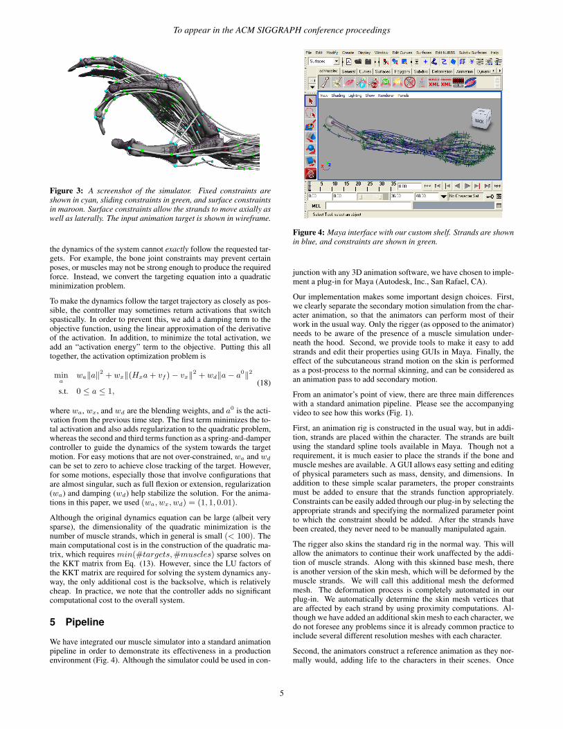
Figure 4: Maya interface with our custom shelf. Strands are shownin blue, and constraints are shown in green.

junction with any 3D animation software, we have chosen to imple-ment a plug-in for Maya (Autodesk, Inc., San Rafael, CA).

Our implementation makes some important design choices. First,we clearly separate the secondary motion simulation from the char-acter animation, so that the animators can perform most of theirwork in the usual way. Only the rigger (as opposed to the animator)needs to be aware of the presence of a muscle simulation under-neath the hood. Second, we provide tools to make it easy to addstrands and edit their properties using GUIs in Maya. Finally, theeffect of the subcutaneous strand motion on the skin is performedas a post-process to the normal skinning, and can be considered asan animation pass to add secondary motion.

From an animator’s point of view, there are three main differenceswith a standard animation pipeline. Please see the accompanyingvideo to see how this works (Fig. 1).

First, an animation rig is constructed in the usual way, but in addi-tion, strands are placed within the character. The strands are builtusing the standard spline tools available in Maya. Though not arequirement, it is much easier to place the strands if the bone andmuscle meshes are available. A GUI allows easy setting and editingof physical parameters such as mass, density, and dimensions. Inaddition to these simple scalar parameters, the proper constraintsmust be added to ensure that the strands function appropriately.Constraints can be easily added through our plug-in by selecting theappropriate strands and specifying the normalized parameter pointto which the constraint should be added. After the strands havebeen created, they never need to be manually manipulated again.

The rigger also skins the standard rig in the normal way. This willallow the animators to continue their work unaffected by the addi-tion of muscle strands. Along with this skinned base mesh, thereis another version of the skin mesh, which will be deformed by themuscle strands. We will call this additional mesh the deformedmesh. The deformation process is completely automated in ourplug-in. We automatically determine the skin mesh vertices thatare affected by each strand by using proximity computations. Al-though we have added an additional skin mesh to each character, wedo not foresee any problems since it is already common practice toinclude several different resolution meshes with each character.

Second, the animators construct a reference animation as they nor-mally would, adding life to the characters in their scenes. Once

5

To appear in the ACM SIGGRAPH conference proceedings

the character has been animated to their liking, the next step is toadd the secondary motion provided by the muscles. The plug-inexports the models, muscle data, and animation keyframes to XMLfiles. The muscle simulator then uses these XML files to recre-ate the Maya scene within the simulation software. The simulatorcalculates the dynamic activation levels for the muscles that bestmatch the animation keyframes provided (Sec. 4). The simulationis then saved as keyframes in an XML file, which are loaded fromour Maya plug-in and baked onto the strand control points. Nowthe Maya strands will move in a biomechanically accurate way.

The simulated rigid body motion is similar, but not identical, to theinput skeletal motion. In the example animations, the average andworst per-vertex reconstruction errors are around 1mm and 5mmrespectively. These reconstructions errors are actually automaticcorrections of physically unattainable motions and configurations.Nevertheless, once the simulation is completed, the animator canchoose to use the new skeletal animation or to stick with the originalinput animation of the rigid bodies, and remap the tendon motionback to the original motion.

Finally, once a strand animation has been imported, the animatorcan use the plug-in to calculate the skin deformation that corre-sponds to the given strand motion. Skin deformation due to sub-cutaneous strands is implemented as a post-process that offsets theskin mesh based on the proximity to strands. The degree of in-fluence of the strands, and hence their visual prominence, can becontrolled by the animator to produce a range of effects.

The skin deformation algorithm is as follows. Every base mesh ver-tex is given a scalar influence weight. This allows us to control theamount of deformation that each deformed mesh vertex undergoes.In our system, these influence weights are painted onto the basemesh using a color set and Maya’s Paint Vertex Color Tool. Onlymesh vertices with positive influence weights are deformed.

At each frame, the closest strand point (ps) to each base mesh ver-tex (pv) is determined. Then the deformed mesh vertex is modifiedas follows:

d = ps − pv

h = max(d · n + c, 0)

f = a exp

(−‖d− (d · n)n‖2

2b2

)pv = pv + (whf)n,

(19)

where n is the outward vertex normal and w is the vertex influenceweight. The parameter a controls the height of the offset, b controlsthe falloff factor in the lateral direction, and c controls the fallofffactor in the normal direction. Thus, when strands protrude above(or lie just beneath) the base skin, each vertex of the deformed skinis moved along its normal by an amount proportional to its distancefrom the strand. The level of deformation is controllable by the in-fluence weights, and by tweaking the height and falloff parameters.

6 Results

The hand model used in our examples contains 54 musculotendonsand 17 bones. The bone and muscle meshes were purchased fromSnoswell Design in Adelaide, and the musculotendon paths wereconstructed based on standard textbook models in the literature[Moore and Dalley 1999]. The skeleton was rigged and animatedby an artist, and the resulting animations were imported into oursimulator, implemented in Java. The activations for an animationsequence of several seconds were computed within a few minutes.

The degrees of freedom of the skeleton are flexion/extension andabduction/adduction of the fingers, thumb, and wrist, and prona-

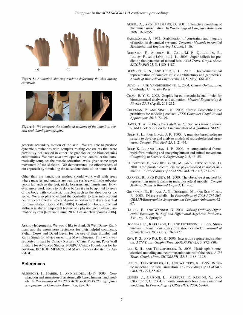
tion/supination of the forearm. Our controller was able to producemotion involving all of these ranges of motion (Fig. 5). Subcuta-neous motions are most pronounced for the extensor and abductortendons of the thumb (Fig. 6), and the extensor digitorum tendonson the back of the palm (Fig. 7). Our technique correctly capturesthe deformation of the skin on the back of the hand during fingerextension (Fig. 8). We can generate more subtle deformation byvarying the skinning parameters (Fig. 6(c)). Finally, we validateour technique by comparing the simulated tendons of the thumb toseveral real thumb photographs (Fig. 9).

(a) (b) (c)

Figure 5: Stillshots from an animation showing prona-tion/supination of the forearm, as well as abduction/adduction ofthe wrist, computed at interactive rates using our controller.

(a) (b) (c)

Figure 6: A frame from the thumb animation, before applying ourmethod (a), and with varying levels of skin deformation (b and c),showing the “anatomical snuffbox”.

(a) (b)

Figure 7: (a) Base skin. (b) With our method applied, showingtendons on the back of the hand realistically deforming the skin.

7 Conclusion and Future Work

We have developed a method for efficient biomechanical simulationof subcutaneous tendons and muscles. The simulation is incorpo-rated into a traditional animation pipeline and can automatically

6

To appear in the ACM SIGGRAPH conference proceedings

(a) (b) (c)

Figure 8: Animation showing tendons deforming the skin duringextension.

Figure 9: We compare the simulated tendons of the thumb to sev-eral real thumb photographs.

generate secondary motion of the skin. We are able to producedynamic simulations with complex routing constraints that werepreviously not tackled in either the graphics or the biomechanicscommunities. We have also developed a novel controller that auto-matically computes the muscle activation levels, given some targetmovement of the skeleton. We demonstrated the effectiveness ofour approach by simulating the musculotendons of the human hand.

Other than the hands, our method should work well with areaswhere muscles and tendons are near the surface with little subcuta-neous fat, such as the feet, neck, forearms, and hamstrings. How-ever, more work needs to be done before it can be applied to areasof the body with volumetric muscles, such as the shoulder or thespine. We also plan to extend the controller to take into accountneurally controlled muscle and joint impedances that are essentialfor manipulation [Kry and Pai 2006]. Control of a body’s tone andstiffness is also an important feature of a physiologically-based an-imation system [Neff and Fiume 2002; Lee and Terzopoulos 2006].

Acknowledgements. We would like to thank Qi Wei, Danny Kauf-man, and the anonymous reviewers for their helpful comments,Stelian Coros and David Levin for the use of their thumbs, andKaran Singh for advice on writing Maya plug-ins. This work wassupported in part by Canada Research Chairs Program, Peter WallInstitute for Advanced Studies, NSERC, Canada Foundation for In-novation, BC KDF, MITACS, and Maya licences donated by Au-todesk.

References

ALBRECHT, I., HABER, J., AND SEIDEL, H.-P. 2003. Con-struction and animation of anatomically based human hand mod-els. In Proceedings of the 2003 ACM SIGGRAPH/EurographicsSymposium on Computer Animation, 98–109.

AUBEL, A., AND THALMANN, D. 2001. Interactive modeling ofthe human musculature. In Proceedings of Computer Animation2001, 167–255.

BAUMGARTE, J. 1972. Stabilization of constraints and integralsof motion in dynamical systems. Computer Methods in AppliedMechanics and Engineering 1 (June), 1–16.

BERTAILS, F., AUDOLY, B., CANI, M.-P., QUERLEUX, B.,LEROY, F., AND LEVQUE, J.-L. 2006. Super-helices for pre-dicting the dynamics of natural hair. ACM Trans. Graph. (Proc.SIGGRAPH) 25, 3, 1180–1187.

BLEMKER, S. S., AND DELP, S. L. 2005. Three-dimensionalrepresentation of complex muscle architectures and geometries.Annals of Biomedical Engineering 33, 5 (May), 661–673.

BOYD, S., AND VANDENBERGHE, L. 2004. Convex Optimization.Cambridge University Press.

CHAO, E. Y. S. 2003. Graphic-based musculoskeletal model forbiomechanical analyses and animation. Medical Engineering &Physics 25, 3 (April), 201–212.

COLEMAN, P., AND SINGH, K. 2006. Cords: Geometric curveprimitives for modeling contact. IEEE Computer Graphics andApplications 26, 3, 72–79.

DAVIS, T. A. 2006. Direct Methods for Sparse Linear Systems.SIAM Book Series on the Fundamentals of Algorithms. SIAM.

DELP, S. L., AND LOAN, J. P. 1995. A graphics-based softwaresystem to develop and analyze models of musculoskeletal struc-tures. Comput. Biol. Med. 25, 1, 21–34.

DELP, S. L., AND LOAN, J. P. 2000. A computational frame-work for simulating and analyzing human and animal movement.Computing in Science & Engineering 2, 5, 46–55.

FALOUTSOS, P., VAN DE PANNE, M., AND TERZOPOULOS, D.2001. Composable controllers for physics-based character ani-mation. In Proceedings of ACM SIGGRAPH 2001, 251–260.

GARNER, B., AND PANDY, M. 2000. The obstacle-set method forrepresenting muscle paths in musculoskeletal models. ComputMethods Biomech Biomed Engin 3, 1, 1–30.

GRINSPUN, E., HIRANI, A. N., DESBRUN, M., AND SCHRCDER,P. 2003. Discrete shells. In Proceedings of 2003 ACM SIG-GRAPH/Eurographics Symposium on Computer Animation, 62–67.

HAIRER, E., AND WANNER, G. 2004. Solving Ordinary Differ-ential Equations II: Stiff and Differential-Algebraic Problems,3 ed., vol. 2. Springer.

HOGFORS, C., KARLSSON, D., AND PETERSON, B. 1995. Struc-ture and internal consistency of a shoulder model. Journal ofBiomechanics 28, 7 (July), 767–777.

KRY, P. G., AND PAI, D. K. 2006. Interaction capture and synthe-sis. ACM Trans. Graph. (Proc. SIGGRAPH) 25, 3, 872–880.

LEE, S.-H., AND TERZOPOULOS, D. 2006. Heads up!: biome-chanical modeling and neuromuscular control of the neck. ACMTrans. Graph. (Proc. SIGGRAPH) 25, 3, 1188–1198.

LEE, Y., TERZOPOULOS, D., AND WALTERS, K. 1995. Realis-tic modeling for facial animation. In Proceedings of ACM SIG-GRAPH 1995, 55–62.

LENOIR, J., GRISONI, L., MESEURE, P., REMION, Y., ANDCHAILLOU, C. 2004. Smooth constraints for spline variationalmodeling. In Proceedings of GRAPHITE 2004, 58–64.

7

To appear in the ACM SIGGRAPH conference proceedings

MAURAL, W., THALMANN, D., HOFFMEYER, P., BEYLOT, P.,GINGINS, P., KALRA, P., AND THALMANN, N. M. 1996. Abiomechanical musculoskeletal model of human upper limb fordynamic simulation. In Proceedings of the 1996 EurographicsWorkshop on Computer Animation and Simulation, 121–136.

MOORE, K. L., AND DALLEY, A. F. 1999. Clinically orientedanatomy, 4 ed. Lippincott Williams & Wilkins.

MURRAY, R. M., LI, Z., AND SASTRY, S. S. 1994. A Mathemat-ical Introduction to Robotic Manipulation. CRC Press.

NEFF, M., AND FIUME, E. 2002. Modeling tension and relax-ation for computer animation. In Proceedings of the 2002 ACMSIGGRAPH/Eurographics Symposium on Computer Animation,81–88.

NG-THOW-HING, V. 2001. Anatomically-based models for phys-ical and geometric reconstruction of humans and other animals.PhD thesis, The University of Toronto.

PAI, D. K. 2002. STRANDS: Interactive simulation of thin solidsusing Cosserat models. In Proceedings of Eurographics 2002,347–352.

PANDY, M. G. 2001. Computer modeling and simulation of humanmovement. Annual Review of Biomedical Engineering, 3, 245–273.

POLLARD, N. S., AND ZORDAN, V. B. 2005. Physically basedgrasping control from example. In Proceedings of the 2005 ACMSIGGRAPH/Eurographics Symposium on Computer Animation,311–318.

QIN, H., AND TERZOPOULOS, D. 1996. D-NURBS: A Physics-Based Framework for Geometric Design. IEEE Transactions onVisualization and Computer Graphics 2, 1, 85–96.

RASMUSSEN, J., DAMSGAARD, M., CHRISTENSEN, S. T., ANDDE ZEE, M. 2005. Anybody - decoding the human muscu-loskeletal system by computational mechanics. Konferanse iberegningsorientert mekanikk (invited paper).

REMION, Y., NOURRIT, J., AND GILLARD, D. 1999. Dynamic an-imation of spline like objects. In Proceedings of the 1999 WSCGConference, 426–432.

SCHEEPERS, F., PARENT, R. E., CARLSON, W. E., AND MAY,S. F. 1997. Anatomy-based modeling of the human musculature.In Proceedings of ACM SIGGRAPH 1997, 163–172.

SHAO, W., AND NG-THOW-HING, V. 2003. A general joint com-ponent framework for realistic articulation in human characters.In Proceedings of the 2003 Symposium on Interactive 3D Graph-ics, 11–18.

SIFAKIS, E., NEVEROV, I., AND FEDKIW, R. 2005. Automaticdetermination of facial muscle activations from sparse motioncapture marker data. ACM Trans. Graph. (Proc. SIGGRAPH)24, 3, 417–425.

SPILLMANN, J., AND TESCHNER, M. 2007. CoRdE: Cosseratrod elements for the dynamic simulation of one-dimensionalelastic objects. In Proceedings of the 2007 ACM SIG-GRAPH/Eurographics Symposium on Computer Animation, 63–72.

TERAN, J., BLEMKER, S., HING, V. N. T., AND FEDKIW, R.2003. Finite volume methods for the simulation of skeletal mus-cle. In Proceedings of the 2003 ACM SIGGRAPH/EurographicsSymposium on Computer Animation, 68–74.

TERAN, J., SIFAKIS, E., BLEMKER, S. S., NG-THOW-HING, V.,LAU, C., AND FEDKIW, R. 2005. Creating and simulatingskeletal muscle from the visible human data set. IEEE Transac-tions on Visualization and Computer Graphics 11, 3, 317–328.

THELEN, D. G., AND ANDERSON, F. C. 2006. Using computedmuscle control to generate forward dynamic simulations of hu-man walking from experimental data. Journal of Biomechanics,39, 1107–1115.

THELEN, D. G., ANDERSON, F. C., AND DELP, S. L. 2002.Generating dynamic simulations of movement using computedmuscle control. Journal of Biomechanics, 36, 321–328.

TSANG, W., SINGH, K., AND FIUME, E. 2005. Helpinghand: an anatomically accurate inverse dynamics solution forunconstrained hand motion. In Proceedings of the 2005 ACMSIGGRAPH/Eurographics Symposium on Computer Animation,319–328.

WATERS, K. 1987. A muscle model for animation three-dimensional facial expression. In Proceedings of ACM SIG-GRAPH 1987, 17–24.

WEINSTEIN, R., GUENDELMAN, E., AND FEDKIW, R. 2008.Impulse-based control of joints and muscles. IEEE Transactionson Visualization and Computer Graphics 14, 1, 37–46.

WILHELMS, J., AND GELDER, A. V. 1997. Anatomically basedmodeling. In Proceedings of ACM SIGGRAPH 1997, 173–180.

WU, F. T. H., NG-THOW-HING, V., SINGH, K., AGUR, A. M.,AND MCKEE, N. H. 2007. Computational representation ofthe aponeuroses as nurbs surfaces in 3d musculoskeletal models.Comput. Methods Prog. Biomed. 88, 2, 112–122.

YIN, K., CLINE, M. B., AND PAI, D. K. 2003. Motion perturba-tion based on simple neuromotor control models. In Proceedingsof Pacific Graphics 2003, 445–449.

ZAJAC, F. 1989. Muscle and tendon: properties, models, scaling,and application to biomechanics and motor control. Crit RevBiomed Eng. 17, 4, 359–411.

ZHU, Q.-H., CHEN, Y., AND KAUFMAN, A. 1998. Real-timebiomechanically-based muscle volume deformation using fem.Computer Graphics Forum 17, 3, 275–284.

ZORDAN, V. B., CELLY, B., CHIU, B., AND DILORENZO, P. C.2004. Breathe easy: model and control of simulated respi-ration for animation. In Proceedings of the 2004 ACM SIG-GRAPH/Eurographics Symposium on Computer Animation, 29–37.

ZORDAN, V. B., MAJKOWSKA, A., CHIU, B., AND FAST, M.2005. Dynamic response for motion capture animation. ACMTrans. Graph. (Proc. SIGGRAPH) 24, 3, 697–701.

8