Inflow and Inflow Plus General purpose pressure and industrial ...
Glasgow Theses Service http://theses.gla.ac.uk/
Murakami, Yoh (2008) A new appreciation of inflow modelling for autorotative rotors. PhD thesis. http://theses.gla.ac.uk/439/ Copyright and moral rights for this thesis are retained by the author A copy can be downloaded for personal non-commercial research or study, without prior permission or charge This thesis cannot be reproduced or quoted extensively from without first obtaining permission in writing from the Author The content must not be changed in any way or sold commercially in any format or medium without the formal permission of the Author When referring to this work, full bibliographic details including the author, title, awarding institution and date of the thesis must be given
i
A New Appreciation of Inflow Modelling for Autorotative Rotors
Yoh Murakami, M.AeroEng
Department of Aerospace Engineering University of Glasgow
July 2008
Thesis submitted to the Faculty of Engineering, University of Glasgow,
in fulfilment of the requirements for the
degree of Doctor of Philosophy.
This thesis is based on research conducted between October 2004 and September 2007
at the Department of Aerospace Engineering, University of Glasgow.
Yoh Murakami
July 2008
© Yoh Murakami, 2008
ii
Abstract
A dynamic inflow model is a powerful tool for predicting the induced velocity
distribution over a rotor disc. On account of its closed form and simplicity, the model is
highly practical especially for studying flight mechanics and designing control systems
for helicopters. However, scant attention has been so far paid to applying this model to
analyse autorotative rotors (i.e. rotors in the windmill-brake state), which differ from
powered helicopter rotors (i.e. rotors in the normal working state) in that the geometric
relation between the inflow and the rotor disc.
The principal aim of this research is to theoretically investigate the applicability of
existing dynamic inflow models for autorotative rotors, and if necessary, to provide a
new dynamic inflow model for autorotative rotors.
The contemporary dynamic inflow modelling is reviewed in detail from first
principles in this thesis, and this identifies a modification to the mass-flow parameter
for autorotative rotors. A qualitative assessment of this change indicates that it is likely
to have a negligible impact on the trim state of rotorcraft in autorotation, but a
significant effect on the dynamic inflow modes in certain flight conditions.
In addition, this thesis includes a discussion about the small wake skew angle
assumption, which is invariably used in the derivation of Peters and He model. The
mathematical validity of the assumption is cast doubt, despite the resultant model has
experimentally been fully validated. This author discusses on a theoretical ground the
possible reason why the Peters and He model works well in spite of its inconsistent
derivation.

iii
Declaration
The author hereby declares that this dissertation is a record of work carried out in the
Department of Aerospace Engineering at the University of Glasgow during the period of
October 2004 to September 2007.
The ideas and results in this dissertation are original in content except where otherwise
stated.
Yoh Murakami
July 2008
iv
Permission to Copy
Yoh Murakami
A New Appreciation of Inflow Modelling for Autorotative Rotors
Department of Aerospace, University of Glasgow
I, the undersigned, request that this thesis should be restricted either to inter-library
lending, to use in another library or to photocopy in part or in full, for three months after
this thesis is finally accepted by the Department of Aerospace Engineering, University
of Glasgow.
After the restriction period, I, the undersigned, am willing that this thesis should be
made available for consultation in the Library of Glasgow University for inter-library
lending, for use in another library or for photocopy in part or in full - at the discretion of
the Librarian - on the understanding that users are made aware of their obligations under
copyright.
Yoh Murakami
July 2008
v
Acknowledgements
I would like to express my sincere appreciation to my supervisor, Dr. Stewart
Houston, for his many hours of advice, constant assistance, supervision and
encouragement.
I need to thank all the people in the department for creating a superb academic
environment. Special thanks must go to Pauline Yearwood, David Suttie, Adriano
Gagliardi, Lucy Schiavetta, Joseph Trchalik, Przemyslaw Marek, Nita Nathan and
Giangicomo Gobbi for their friendship and encouragement.
I would also like to thank all of my friends in Glasgow, especially members of the
Kelvin Ensemble, Glasgow Orchestra Society, St. Vincent Baroque Players, Harts String
Quartet and Stone String Quartet for their having provided me with a wonderful musical
life (music has always been the best pastime), and Rinako Nakagawa and Taro Fujita for
their friendship and invaluable help.
I would also like to express my heartfelt gratitude to Dr. Darren Wall and Dr. Douglas
Thomson, who patiently proof-read the final draft.
I also have to express my profound gratitude in this edition to Dr. Roy Bradley, who
was the external examiner, and Dr. Eric Gillies, the internal, for their tough and strict
but professional and instructive examination, suggestions and advice. When looking
back to this experience in some decades, my gratitude shall be more profound; at least I
must make my own future so that I can feel so both for them and myself.
Last but not least, I would like to express my deepest gratitude to my mother, Luna,
who encouraged me and supported my study at all times in every aspect.
This work shall simply be dedicated to her.
Yoh Murakami
July 2008
Contents
Abstract ii
Declaration iii
Permission to Copy iv
Acknowledgements v
Contents vi
Nomenclature x
Acronyms and Abbreviations x
General x
Superscripts xi
Subscripts xi
Latin Symbols xi
Greek Symbols xiv
List of Figures xvii
List of Tables xix
Chapter 1 Introduction
1.1 Overview 1
1.2 Organisation of this Thesis 1
1.3 Focus of this Thesis 3
1.4 General Introduction to the Dynamic Inflow Model 4
1.4.1 Base Principles 5
1.4.2 The Characteristics of the Dynamic Inflow Model 6
1.5 Concise History of the Attempts to Describe the Induced Flow
Distribution 9
1.5.1 From Classical Theory to the Pitt and Peters Model 9
1.5.2 Lift Deficiency Function 16
1.5.3 Computational Method 19
1.5.4 From the Pitt and Peters Model to the State of the Art 21
1.6 Literature on Autorotation 25
vii
Chapter 2 Review of the Dynamic Inflow Model of Peters and He
2.1 Introduction 28
2.1.1 Overview 28
2.1.2 Notations 28
2.2 Review of the Dynamic Inflow Model of Peters and He 29
2.2.1 Fundamental Assumptions for the Mathematical
Derivation of the Peters and He Model 29
2.2.2. The Representation of the Pressure Field 30
2.2.3. Normalisation of the Pressure Function 34
2.2.4. The Relation between the Pressure Function and the
Induced Velocity 36
2.2.5 Matrix Representations 38
2.2.6 The Unified Representation of the Induced Flow Fields 41
2.2.7 The Apparent Mass Matrix, M 46
2.2.8. The Gain Matrix, L - part 1
- The General Representation 48
2.2.9 The Gain Matrix, L - part 2
- Skewed Cylindrical Representation for the Wake Tube 51
2.2.10 The Gain Matrix, L - part 3
- The Pressure Function 54
2.2.11 The Gain Matrix, L - part 4
- The Small Wake Skew Angle Assumption 55
2.2.12 The Gain Matrix, L - part 5
- The Elements in Closed Forms 60
2.3 The Pitt and Peters model 63
2.3.1 The Apparent Mass Matrix, M 63
2.3.2 The Gain Matrix, L 67
2.4 The Mass-flow Parameter and Non-linear Versions 68
2.5 Discussion 71
2.6 Chapter Summary 72
viii
Chapter 3 Dynamic inflow modelling for autorotative rotors
- The Geometric Difference in the Autorotative Rotors from those Rotors in the Normal
Working State
3.1 Introduction 73
3.2 The Applicability of the Dynamic Inflow Model
to an Autorotative Rotor 74
3.2.1 Examination on Matrix Elements of Dynamic Inflow Models 74 3.2.2 Definitions of the Wake Skew Angle 75 3.2.3 Examination on the Mass-flow Parameter 76
3.2.4 Unified form of Vm+ and Vm 77
3.3 Numerical Simulation 78
3.4 Results from Numerical Simulation 80
3.5 Analysis of the Results Obtained 92
3.6 Discussion 93
3.7 Chapter Summary 95
Chapter 4 Consideration of the Small Wake Skew Angle Assumption
4.1 Introduction 97
4.2 New Gain Matrix Model 97
4.2.1 Derivation of a New No-Assumption Model 97
4.2.2 The Modified Pitt and Peters Model 99
4.2.3 Numerical Simulation 100
4.3 Further Discussion 106
4.3.1 Deductive and Inductive Approaches 106
4.3.2 Characteristics of the Gain Matrix Elements of the Peters and He Model
110
4.3.3 The Pitt and Peters Model and the Edgewise Flight Case 112
4.3.4 How the Small Wake Skew Angle Assumption Works 119
4.4 Chapter Summary 122
Chapter 5 Conclusions and Future Directions
5.1 Introductory Remarks - Review of the Research Aim and Objectives 124
5.2 Conclusions 125
5.3 Future Direction 128
5.4 Conclusive Remarks 129
ix
Appendices
Appendix 2.1 Linearisation of the Euler Equation 130
Appendix 2.2 Transformation from Cartesian to Polar Coordinates on the Rotor 130
Appendix 2.3 The Ellipsoidal Coordinate System 131
Appendix 2.4 Prandtl’s Potential Function 134
Appendix 2.5 The Associated Legendre Functions 135
Appendix 2.6 The Legendre Functions 140
Appendix 2.7 A Complement to Eq. (2.38) 142
Appendix 2.8 Comments on the Coefficients of Lrmcjn and Lrmsjn 142
Appendix 2.9 Variation in the Representation of the Pressure Potential 144
Appendix 3.1 Further Discussion about the Mass-flow Parameter 146
Appendix 3.2 Forces and Moments on a Blade Element 147
References 149
x
Nomenclature
Acronyms and Abbreviations ARAIC Aircraft and Railway Accidents Investigation Commission (of Japan)
ARMCOP ARMy heliCOPter CAA Civil Aviation Authority
CFD Computational Fluid Dynamics
DIY Do It Yourself
DOF Degree Of Freedom
KIAS Knots, Indicated Air Speed
NACA National Advisory Committee for Aeronautics
NASA National Aeronautics and Space Administration
ONERA Office National d’Études et de Recherches Aérospatiales
RASCAL Rotorcraft Aeromechanics Simulation for Control AnaLysis
STOL Short Take-Off and Landing
VTOL Vertical Take-Off and Landing
General 0 zero vector
n!! double factorial, n!! = n(n 2)(n 4) x variable
x vector variable with implicit representation of elements
(column vectors unless otherwise defined) tx transposed vector of x
(xi) column vector variable with explicit representation of elements
dx infinitesimal variable
[X] matrix variable with implicit representation of elements
[X]1 inverse matrix of [X]
X[xij] matrix variable with explicit representation of elements
Xmn polynomials defined by two indices, m and n
xi
Superscripts x non-dimensionalised quantity
x derivative of xwith respect to non-dimensional time, ∂x/∂t
xc indication of cosine
x(c) indication of the convective part of the Euler equation
xm, xr terms associated with m -th or r-th harmonics
x(M), x(L) indication of apparent mass and gain matrices
xs indication of sine
x(t) indication of the time-derivative part of the Euler equation
Subscripts x0 indication of steady state; or indication of a value on rotor disc
xn, xj terms associated with n -th or j-th polynomials
xx, xy, xz indication of coordinates
Latin Symbols a = acceleration, m/s2
arj, brj = Fourier coefficients for the representation of induced velocity
an, bn = arbitrary Fourier coefficients
ahingex , ahingez = hinge acceleration components, m/s2
A = rotor area, m2
[A] = transformation matrix, Armjn=∫
0
1 PrjΨmn d
[A] = linearised model system matrix
b = number of blades
[B] = transformation matrix, Brmjn=∫
0
1(1/)PrjPmn d
[B] = linearised model control matrix
c = blade chord, m
cr = blade root-cut, m
C = linear operator representation of ∂/∂z
C(k) = Theodorsen’s lift deficiency function
CL, CM = aerodynamic perturbations in roll and pitch moment,
xii
non-dimensionalised on Ω20R5
C2L, C2M = second harmonic aerodynamic perturbations in roll and pitch moment, non-dimensionalised on Ω2
0R5
Cmn , Dmn = Fourier coefficients for Prandtl’s potential function
CT = aerodynamic perturbation in thrust, non-dimensionalised on Ω20R5
D = drag, non-dimensionalised on Ω20R4
D = linear operator representation of (1/V)∫
∞0∂z
∂ ....d$
e, eψ, e& = unit base vectors in ellipsoidal coordinates
f = function defined as f() =∫
∞0
∂r
∂+
r
m
Pmn ()Qmn ()dz
F = force, N
F = force vector, N
h1, h2, h3 = metric factors
Hmn = coefficient defined as Hm
n = (n +m 1)!!(n m 1)!!/[(n +m)!!(n m)!!]
i = imaginary number, i = 1√
Iflap, Ipitch, Ilag = blade inertia, Nm2
Ixx, Iyy, Izz, Ixz = rotor inertia, Nm2
J = function defined as J = [(1 + &2)(1 2) y20](1 y2
0 2
0)
√
K = function defined as K = &2(&2 + 1) + 20(&2 + 1)cos2 1 &2y2
0sin2 1
[K] = matrix representation of C1 Kc = longitudinal gradient of the induced flow distribution in Glauert’s model
Kc, Ks = lateral and longitudinal wake curvatures
KR = wake curvature
Kmn = coefficient, Km
n = (2/2)Hmn
L = lift, non-dimensionalised on Ω20R4
[L] = gain matrix
[L ] = gain matrix excluding the mass-flow parameter in the definition
L = aerodynamic moment vector, Nm
m = mass, kg
m = rotor mass, kg
M = mass of aircraft, kg
[M] = apparent mass matrix
xiii
Mflap, Mpitch,Mlag = moment acting on a blade, Nm
P = pressure, kg/ms2
Pn = the Legendre function of the first kind
Pmn = the associated Legendre function of the first kind
p, q, r = perturbed angular velocity components along airframe axes, rad/s
pn, qn = polynomials, defined as pn(x) = 1 2!
n(n+1)x2 +
4!
(n2)n(n+1)(n+3)x4 ,
qn(x) = x 3!
(n1)(n+2)x3 +
5!
(n3)(n1)(n+2)(n+4)x5 .
q = perturbed velocity vector, q = (u, v, w), non-dimensionalised on Ω0R
Qn = the Legendre function of the second kind
Qmn = the associated Legendre function of the second kind
r = radial position on rotor disc, m
rcg = position of centre of mass, m
rhinge = position of flap, lag and feather hinge, m
rhub = position of rotor hub, m
r, ψ, z = cylindrical coordinates
R = rotor radius, m
R = set of real numbers
t = time, s
t = tan1
[T1], [T2], [T3] = transformation matrices
u = velocity vector, m/s
u = control vector
U = total velocity vector, non-dimensionalised on Ω0R
u, v, w = perturbed velocity components along airframe axes,
non-dimensionalised on Ω0R
v = dimensional induced velocity, m/s
v0 = dimensional uniform induced velocity, m/s
vi = dimensional induced velocity, m/s
v1s = dimensional induced velocity component, longitudinal, m/s
v1c = dimensional induced velocity component, lateral, m/s
vm = dimensional mass-flow parameter, m/s
vm+ = dimensional mass-flow parameter for normal working state, m/s
vm = dimensional mass-flow parameter for windmill-brake state, m/s
V = modulus of V, V = |V| V = steady velocity vector, non-dimensionalised on Ω0R, V = (Vx, Vy, Vz)
xiv
V = arbitrary vector function, V = (V1, V2, V3)
Vm = mass-flow parameter, dimensionless on Ω0R
Vm+ = mass-flow parameter for normal working state, dimensionless on Ω0R
Vm = mass-flow parameter for windmill-brake state, dimensionless on Ω0R
Vm = unified form of Vm+ and Vm, dimensionless on Ω0R
VT = non-dimensional total flow at rotor disc, dimensionless on Ω0R
V∞ = free stream speed, non-dimensionalised on Ω0R
x = variable for functions in general
x = state vector
x, y, z = rotor disc coordinates, non-dimensionalised on R
X = wake skew angle parameter, tan(1/2)
X = rotor force vector, X = (X, Y, Z), N Xelem,X
aero
elem,Xinert
elem
= blade element contributions to rotor force: total, aerodynamic, inertial, N
y = arbitrary function of x , y = y(x)
ycg = position of the centre of gravity
[Y] = matrix representation of D
Y = extended wake skew angle parameter
in the no-assumption model
Greek Symbols : = angle between free stream and rotor disc, rad
:e = effective rotor angle of attack, :e = (2/2) 1, rad
:mn = Fourier coefficients for induced velocity, cosine part
; = flapping angle, rad
;mn = Fourier coefficients for induced velocity, sine part
Γ = Gamma function
Γrmjn
= coefficient defined as Γrmjn=∑
l=r+1
∞ArjlΛrmln
< = drag coefficient
<ij = Kronecker’s delta
<r = rudder angle, deg
= = lag angle, rad
=mn = Fourier coefficients for the induced velocity, cosine part
&c = lateral stick position, % (0% fully left)
xv
&s = longitudinal stick position, % (0% fully forward)
> = collective pitch angle, deg
> = perturbed pitch attitude, deg
>1s = longitudinal cyclic pitch , rad
>1c = lateral cyclic pitch, rad
>s = longitudinal tilt of the rotor shaft with respect to the airframe, rad
? = non-dimensional total inflow
?0 = non-dimensional induced flow component, mean
?1s = non-dimensional induced flow component, longitudinal
?1c = non-dimensional induced flow component, lateral
?f = free stream inflow, V sin:
?m = non-dimensional inflow die to the rotor thrust
Λrmjn
= integral defined as Λrmjn=∫
0
1 Prj()∫
∞0
∂r
∂+
r
m
Pmn ()Qmn ()dzd
@ = advance ratio in rotor coordinates, Vcos:
@3 = axial component of inflow, V sin:
= kinetic viscosity
, ψ, & = ellipsoidal coordinates
$ = coordinate along free stream, positive upstream
= density of air, kg/m3
mn = non-dimensionalising factor for Pmn , mn = 2n+11
(nm)!(n+m)!
√
[A] = time-constant matrix, [L][M] Amn = pressure coefficient
B = perturbed roll attitude, deg
Bs = lateral tilt of the rotor shaft with respect to the airframe, rad Φ = pressure potential, non-dimensionalised on R4Ω2
0
Φ(t) = pressure potential corresponding to time-derivative terms in the Euler equation, non-dimensionalised on R4Ω2
0
Φ(c) = pressure potential corresponding to convection terms in the Euler equation, non-dimensionalised on R4Ω2
0
Φ! = pressure potential for the Pitt and Peters model, non-dimensionalised on R4Ω2
0
1 = wake skew angle, rad
ψ = rotor azimuth, rad
ψ = perturbed roll attitude, deg

xvi
Ψmn = general expansion function
ω = non-dimensionalised induced velocity
ωx, ωy, ωz = blade angular velocities, m/s
mn = Fourier coefficients for the induced velocity, sine part
Ω = rotor speed, rad/s
Ωp = propeller speed, rad/s
xvii
List of Figures Fig. 1-1 [The first principle of the dynamic inflow model.] 5
Fig. 1-2 [Schematic diagram for the typical use of the dynamic inflow model.] 8
Fig. 1-3 [Comparison between the uniform distribution and Glauert’s model.] 10
Fig. 1-4 [Gyroplanes: C.4 and G7-R447.] 26
Fig. 2-1 [Vehicle coordinate systems; Helicopter and Gyroplane.] 31
Fig. 2-2 [Difference in the aerodynamic configuration of
the rotors of normal working and windmill-state states.] 32
Fig. 2-3 [Difference in the rotor angle of attack of helicopter and gyroplane rotors.] 32
Fig. 2-4 [Matrix representation of C1 .] 39
Fig. 2-5 [Skewed cylinder for the rotor wake.] 49
Fig. 2-6 [Wake tube description by the vortex transportation method.] 49
Fig. 2-7 [Lift distributions on a blade described by the associated Legendre function;
the first and second harmonics.] 64
Fig. 2-8 [Inflow components in the wind axes.] 69
Fig. 3-1 [Montgomerie (left) and Westland Puma (right).] 80
Fig. 3-2 [Comparison of forward flight speed and mass-flow parameters,
Montgomerie.] 82
Fig. 3-3 [Comparison of forward speed and inflow components, Montgomerie.] 82
Fig. 3-4 [Comparison of forward speed and airframe attitude, Montgomerie.] 83
Fig. 3-5 [Comparison of descent rate and inflow components
at 50 knots, Montgomerie.] 83
Fig. 3-6 [Comparison of descent rate and airframe attitude at 50 knots,
Montgomerie.] 84
Fig. 3-7 [Comparison of descent angle and flight controls, Montgomerie.] 84
Fig. 3-8 [Comparison of forward flight speed and flight controls, Montgomerie.] 85
Fig. 3-9 [Comparison of forward flight speed and mass-flow parameters
with collective pitch at 6.5 , Puma in the windmill-brake state.] 85
Fig. 3-10 [Comparison of inflow velocity for Vm+ and Vm
with collective pitch at 6.5 , Puma in the windmill-brake state.] 86
Fig. 3-11 [Comparison of descent rate and airframe attitude, Puma.] 87
Fig. 3-l2 [Comparison of Forward Flight Speed and Flight Controls, Puma.] 87
Fig. 3-13 [Comparison of lateral inflow component for Vm+ and Vm.] 88
Fig. 3-14 [Lateral inflow mode; comparison for Vm+ and Vm.] 89
xviii
Fig. 3-15 [Coupled uniform/longitudinal inflow modes;
comparison for Vm+ and Vm.] 89
Fig. 4-1 [Comparison of collective pitches against forward flight speed.] 100
Fig. 4-2 [Comparison of longitudinal cyclic pitches against forward flight speed.] 101
Fig. 4-3 [Comparison of lateral cyclic pitches against forward flight speed.] 101
Fig. 4-4 [Comparison of roll attitudes against forward flight speed.] 102
Fig. 4-5 [Comparison of pitch attitudes against forward flight speed.] 102
Fig. 4-6 [Comparison of wake skew angles against forward flight speed.] 103
Fig. 4-7 [Comparison of uniform components of induced velocity against forward flight
speed.] 103
Fig. 4-8 [Comparison of the longitudinal components of induced velocity against
forward flight speed.] 104
Fig. 4-9 [Comparison of modes.] 105
Fig. 4-10 [Comparisons of trigonometric parts in the gain matrices.] 110
Fig. 4-11 [Trigonometric parts based on the small wake skew angle assumption.] 111
Fig. 4-12 [Integral Domains of the $-axis for the Edgewise Flight Case.] 114
Fig. A2-1 [The ellipsoidal coordinate system.] 131
Fig. A2-2 [The associated Legendre functions of the first kind.] 135
Fig. A2-3 [Real parts of the associated Legendre functions of the second kind.] 138
Fig. A2-4 [Imaginary parts of the associated Legendre functions
of the second kind.] 138
Fig. A2-5 [The Legendre functions of the first and second kinds.] 141
xix
List of Tables Table 2-1 [Examples of Mm
n ] 48
Table 3-1 [Specification of the Montgomerie and Puma.] 81
Table 3-2 [Linearised system eigenvalues - Vm+;
35 KIAS, 3500 feet/min. vm = 3.6 m/s.] 90
Table 3-3 [Linearised system eigenvalues - Vm;
35 KIAS, 3500 feet/min. vm = 14.3 m/s.] 90
Table 3-4 [Linearised system eigenvalues - Vm+;
40 KIAS, 2250 feet/min. vm = 18.2 m/s.] 91
Table 3-5 [Linearised system eigenvalues - Vm;
40 KIAS, 2250 feet/min. vm = 20.6 m/s.] 91
Chapter 1 Introduction
1
Chapter 1
Introduction
1.1 Overview The primary aim of this thesis is to theoretically investigate the applicability of
existing dynamic inflow models for autorotative rotors. Contemporary dynamic inflow
models such as the Pitt and Peters model(1) have been developed for helicopter rotors in
the normal working state. The literature suggests that this would be the first time that
the possibility of applying the dynamic inflow model to autorotative rotors has been
examined from a theoretical viewpoint.
Ever since the first gyroplane, Model C.4 designed by Juan de la Cierva, flew in
1923(2,3,4), it has always been a major problem how to describe the distribution of the
airflow around the rotor. Although simple momentum theory can provide a key insight
into the rotor performance in steady axial flight(5,6), a more sophisticated description
about the inflow distribution is required to study the rotor performance, rotor stability
and controllability in unsteady state or in forward flight, and to evaluate rotor loads,
which are closely connected with the controls. The rotor loads are important also in
relation to rotor vibration and structural fatigue. Historically, a variety of methods have
been proposed to describe the detailed inflow distribution over rotors in the normal
working state, either in steady or unsteady state for either axial or forward flight.
Examples thereof include various dynamic inflow models.
In the following Sections in this Chapter, the characteristic features and historical
development of the dynamic inflow model will be outlined. The discussion of this thesis
shall mainly be focused on theoretical and mathematical aspects, but some numerical
verification of the salient points are to be presented.
1.2 Organisation of this Thesis An extensive literature review is given in Chapter 1 in relation to dynamic inflow
models such as the Pitt & Peters and Peters & He models. In an attempt to outline the
characteristic features of dynamic inflow modelling, the practical applications and
Chapter 1 Introduction
2
historical development are shown in comparison with other methods, such as lift
deficiency functions and CFD methods. Furthermore, a brief history of gyroplanes and a
description of the current problems in the field of gyroplane research are introduced so
as to make clear the significance of this research.
In Chapter 2, the mathematical derivation of Peters and He model is carefully
examined aiming to theoretically identify the necessary modifications to the model for
its application to autorotative rotors. In this examination, the author seeks to improve
the lucidity of the derivation of these models by examining the assumptions they are
based on, presenting proofs to related theorems, as well as offering new approaches to
interpreting these methods. A few potentially misleading typographical error in the
original literature are also detailed. Although the author enunciates his own point of
view in places, it must be herein emphasised that the results and derivations presented in
this Chapter fundamentally rely on the work contained in Dr. C.-J. He’s doctoral
thesis(7).
In Chapter 3, the applicability of the existing dynamic inflow model for autorotative
rotors is considered, and the necessary modification to the model for such applications
are presented in terms of the geometric difference between rotors in the normal working
and windmill-brake states with regard to the relation between the rotor angle of attack
and the incoming flow. This difference always exists between rotors in those two states.
Some computational simulations are also conducted to study the affect of the
modification made in the mass-flow parameter.
In Chapter 4, the small wake skew angle assumption, which is a vital requirement in
the derivation of Peters and He model, is examined. The analysis of Chapter 4 is based
on that of Chapter 2, but the results are not limited to autorotative rotors. An alternative
model, in which the small wake skew angle assumption is not used, is also presented.
The reason why the Peters and He model practically works so well in spite of the
questionable assumption is discussed on a theoretical ground.
In Chapter 5, an overview and discussion of the results presented in this thesis are
provided together with recommendations for future research directions.
Chapter 1 Introduction
3
1.3 Focus of this Thesis The primary focus of this research is the improvement of the performance of existing
gyroplanes and the clarification of the dynamic behaviour of these aircraft. Following
the advent of the helicopter1, the gyroplane gradually gave way to the helicopter, and
only a small number of studies were undertaken either on an academic, military or
governmental basis after the Second World War2. In the mean time, the gyroplane has
been developed generally by amateur home-builders and some small companies for
sports or leisure flying, and consequently, a good number of pilots were killed in
accidents without amply clarifying the possible causes of such accidents. Some fatal
accidents could have been attributed to human error or technical malfunctions owing to
inexpert weekend DIY manufacturing, but other accidents might have been caused by
more fundamental design faults, or the control system. As the dead cannot speak in their
own defence, it may be attributed to the authorities that closer investigations into the
possible causes have not been pursued.
In the United Kingdom, CAA decided to ground all gyroplanes produced by Air
Command International Inc. in 1991 after a series of six fatal accidents resulting in
seven fatalities from 1989 to 1991, and this became the trigger for a series of research
studies on gyroplanes at the University of Glasgow(8,9,10). (Some accident reports in the
U.K. are available from Ref. (11).) Compared to the U.K. and the U.S.A., where the
gyroplane is relatively popular, the public recognition of the danger of gyroplanes is
much smaller in other countries, and legislative systems such as airworthiness
certificates and relevant air traffic laws can also be less developed.
For example, in Japan, where no official licensing system is set up for the gyroplane,
there were 23 accidents between 1974 and 2006, including 8 accidents involving Air
Command Gyroplanes, with 18 pilots killed. Given that there are only 120 or so
officially registered gyroplanes in Japan, this accident rate is clearly significant. The
Secretariat of ARAIC concluded that 19 accidents thereof could simply be attributed to
human error and 1 to improper maintenance(12). Considering the fact that all Air
1 It is controversial to whom the title of the first inventor of the helicopter should be credited. Two Frenchmen, Louis Breguet (1880-1955) and Paul Cornu (1881-1944), independently insisted that they flew in 1907, but it is rather doubtful that their machines had enough power to take off. A Dane, Jens Ellehammer (1871-1946), flew in 1913, with the Crown Prince of Denmark witnessing the flight. It is more popularly accepted that the first flight is credited either to Focke Fw.61 in 1936(13,14) or to Breguet-Dorand’s Gyroplane Laboratoire in 1935. In any case, the helicopter was not practical maturity until Sikorsky’s Type R-4 was put into production in 1942(15). 2 Quite a few research studies were made before the Second World War including Refs. (2-4,16-22). However, the number of such works published after the war is considerably few. References (23) and (24) are two such rare examples of studies undertaken after the Second World War before 1991.
Chapter 1 Introduction
4
Command Gyroplanes have been grounded in the U.K. due to the possible inherent
instability, one may consider that there is a possibility that some of the accidents in
Japan could be attributed to the inherent flight characteristics of the vehicles rather than
human error.
There is thus a requirement to improve the basic understanding of the gyroplane
aeromechanics, with both theoretical and experimental approaches necessary for this
aim. In order to study flight mechanics of the gyroplane, a mathematical model of the
induced velocity for autorotative rotors is an absolute necessity, and the dynamic inflow
model should be better suited to this modelling task than other approaches to describing
the inflow distribution, including various CFD methods. This forms the principal
motivation for the present research.
As well as addressing safety issues as described above, there is also a belief that
gyroplanes can still compete with other classes of V/STOL aircraft, including
helicopters and tilt rotors, as a short-range transport of the future, and several projects to
explore this possibility are presently under way. Thus, it is believed that a wide range of
basic research, either theoretical or experimental, is necessary at this stage to realise
those projects in time to come. Based on the view above, the possible contribution to the
further development in gyroplanes also partly motivated this research.
Furthermore, autorotation is also of great importance for helicopters as the way of
emergency landing, though it is an abnormal condition. Nevertheless, scant attention is
paid to either the theoretical or experimental investigation, and this situation needs a
suitable mathematical model which can be used in control analysis. Hence, further
research on the flight state of autorotation should be meaningful not only for gyroplanes
but also for helicopters in autorotation.
This background forms the motivation for this work, and it is hoped that this research
will contribute to the study of control system and flight dynamics for the gyroplane and
the autorotative state of the helicopter.
1.4 General Introduction to the Dynamic Inflow Model In the following Subsections, the base principles of the dynamic inflow model and an
outline of the schematic application thereof are briefly reviewed prior to Chapter 2, in
Chapter 1 Introduction
5
which the model will be derived and examined in depth from a rigorous mathematical
perspective. The understanding of base principles beforehand is believed to make it
easier to understand later Chapters. Also, it is aimed that the characteristic features of
the dynamic inflow model are generally elucidated in comparison with other methods
for describing the induced flow distribution over a rotor disc.
1.4.1 Base Principles
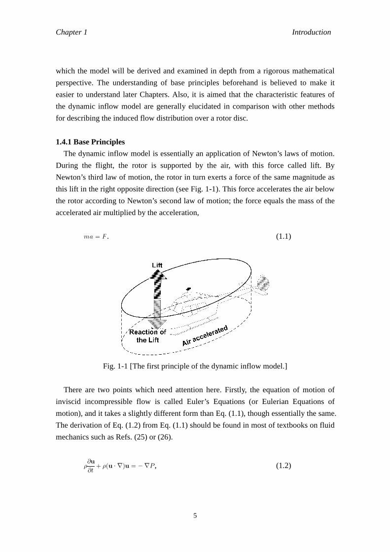
The dynamic inflow model is essentially an application of Newton’s laws of motion.
During the flight, the rotor is supported by the air, with this force called lift. By
Newton’s third law of motion, the rotor in turn exerts a force of the same magnitude as
this lift in the right opposite direction (see Fig. 1-1). This force accelerates the air below
the rotor according to Newton’s second law of motion; the force equals the mass of the
accelerated air multiplied by the acceleration,
ma = F . (1.1)
Fig. 1-1 [The first principle of the dynamic inflow model.]
There are two points which need attention here. Firstly, the equation of motion of
inviscid incompressible flow is called Euler’s Equations (or Eulerian Equations of
motion), and it takes a slightly different form than Eq. (1.1), though essentially the same.
The derivation of Eq. (1.2) from Eq. (1.1) should be found in most of textbooks on fluid
mechanics such as Refs. (25) or (26).
∂t
∂u+ (u ∇)u = ∇P , (1.2)
Chapter 1 Introduction
6
where u , t , and P denote fluid velocity, time, fluid density and pressure,
respectively.
Secondly, the total mass of the air flow accelerated is not as straightforward as in the
motion of point masses, and thus the determination of the apparent mass of the flow
forms a problem that must also be considered. Still, the reader should be encouraged to
remember that the dynamic inflow model is in essence simply an application of
Newton’s laws of motion. Note that when applying Eq. (1.1) or (1.2), the rotor may be
regarded as a thin flat continuous surface, which accelerates the air underneath the rotor
to generate discontinuities in the pressure and velocity between upper and lower sides
thereof. This assumption is called actuator disc theory.
The dynamic inflow model is typically represented in the form of a matrix equation.
[M] u + [L]1u = F , (1.3)
where u and F are state vectors of the induced flow and the lift (rotor thrust and
moments)3, a dot (.) denotes differentiation with respect to time, ∂/∂t. At this stage, it
may be noted that Eq. (1.3) is, very roughly speaking, in the same form as of Eq. (1.2),
which is itself a rewriting of Eq. (1.1) for an ideal fluid. (Note that since the differential
operators of ∂/∂t is linear, it can be expressed as a matrix in Hilbert space. However,
the differential operator of (u ∇) in Eq. (1.2) is not linear, and hence it should be
invariably linearised to result in a linear form.) Given Newton’s laws of motion, the
derivation of the dynamic inflow model in the form of Eq. (1.3) from Eq. (1.2) is thus
straightforward. Note that the [M] and [L] matrices in Eq. (1.3) are conventionally
called apparent mass matrix and gain matrix, and their product, [A] = [L][M] , is called
time constant matrix. These epithets will be occasionally used also in this thesis.
1.4.2 The Characteristics of the Dynamic Inflow Model
In this Section, a general appraisal of the dynamic inflow model is described, aiming
to sketch out its features (i.e., strength, weakness, usefulness, limitation, etc.) in a
practical context compared to other models. The characteristic features of the dynamic
inflow model can be outlined as follows:
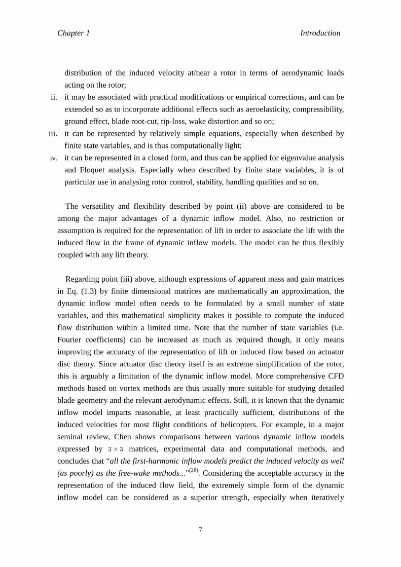
i. the dynamic inflow model is a mathematical model describing the unsteady dynamic
3 It is difficult to identify who first introduced the matrix form because the dynamic inflow model was developed by many researchers in a parallel manner in the early stages. Reference (27) is one of the earliest works in which the matrix form is used, and Ref. (1) is believed to be most instrumental in establishing the matrix form.
Chapter 1 Introduction
7
distribution of the induced velocity at/near a rotor in terms of aerodynamic loads
acting on the rotor;
ii. it may be associated with practical modifications or empirical corrections, and can be
extended so as to incorporate additional effects such as aeroelasticity, compressibility,
ground effect, blade root-cut, tip-loss, wake distortion and so on;
iii. it can be represented by relatively simple equations, especially when described by
finite state variables, and is thus computationally light;
iv. it can be represented in a closed form, and thus can be applied for eigenvalue analysis
and Floquet analysis. Especially when described by finite state variables, it is of
particular use in analysing rotor control, stability, handling qualities and so on.
The versatility and flexibility described by point (ii) above are considered to be
among the major advantages of a dynamic inflow model. Also, no restriction or
assumption is required for the representation of lift in order to associate the lift with the
induced flow in the frame of dynamic inflow models. The model can be thus flexibly
coupled with any lift theory.
Regarding point (iii) above, although expressions of apparent mass and gain matrices
in Eq. (1.3) by finite dimensional matrices are mathematically an approximation, the
dynamic inflow model often needs to be formulated by a small number of state
variables, and this mathematical simplicity makes it possible to compute the induced
flow distribution within a limited time. Note that the number of state variables (i.e.
Fourier coefficients) can be increased as much as required though, it only means
improving the accuracy of the representation of lift or induced flow based on actuator
disc theory. Since actuator disc theory itself is an extreme simplification of the rotor,
this is arguably a limitation of the dynamic inflow model. More comprehensive CFD
methods based on vortex methods are thus usually more suitable for studying detailed
blade geometry and the relevant aerodynamic effects. Still, it is known that the dynamic
inflow model imparts reasonable, at least practically sufficient, distributions of the
induced velocities for most flight conditions of helicopters. For example, in a major
seminal review, Chen shows comparisons between various dynamic inflow models
expressed by 3 3 matrices, experimental data and computational methods, and
concludes that “all the first-harmonic inflow models predict the induced velocity as well
(as poorly) as the free-wake methods...” (28). Considering the acceptable accuracy in the
representation of the induced flow field, the extremely simple form of the dynamic
inflow model can be considered as a superior strength, especially when iteratively
Chapter 1 Introduction
8
conducting real-time simulations4.
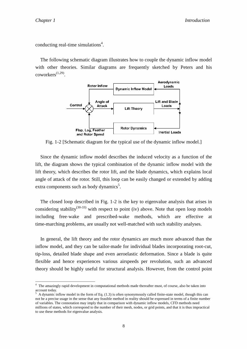
The following schematic diagram illustrates how to couple the dynamic inflow model
with other theories. Similar diagrams are frequently sketched by Peters and his
coworkers(1,29).
Fig. 1-2 [Schematic diagram for the typical use of the dynamic inflow model.]
Since the dynamic inflow model describes the induced velocity as a function of the
lift, the diagram shows the typical combination of the dynamic inflow model with the
lift theory, which describes the rotor lift, and the blade dynamics, which explains local
angle of attack of the rotor. Still, this loop can be easily changed or extended by adding
extra components such as body dynamics5.
The closed loop described in Fig. 1-2 is the key to eigenvalue analysis that arises in
considering stability(30-33) with respect to point (iv) above. Note that open loop models
including free-wake and prescribed-wake methods, which are effective at
time-marching problems, are usually not well-matched with such stability analyses.
In general, the lift theory and the rotor dynamics are much more advanced than the
inflow model, and they can be tailor-made for individual blades incorporating root-cut,
tip-loss, detailed blade shape and even aeroelastic deformation. Since a blade is quite
flexible and hence experiences various airspeeds per revolution, such an advanced
theory should be highly useful for structural analysis. However, from the control point
4 The amazingly rapid development in computational methods made thereafter must, of course, also be taken into account today. 5 A dynamic inflow model in the form of Eq. (1.3) is often synonymously called finite-state model, though this can not be a precise usage in the sense that any feasible method in reality should be expressed in terms of a finite number of variables. The connotation may imply that in comparison with dynamic inflow models, CFD methods need millions of states, which correspond to the number of their mesh, nodes, or grid points, and that it is thus impractical to use these methods for eigenvalue analysis.
Chapter 1 Introduction
9
of view, it is more important that there should be a balance between each theory shown
in Fig. 1-2, because it is often the case that the combination of crude models yields
better stability analysis results than those found for a crude model coupled with a
detailed model6(34-36). It is regrettable that these advanced blade dynamic models should
be still often used in combination with simple momentum theory or quasi-steady inflow
model. Examples of more advanced inflow models popularly used today include the Pitt
and Peters model(1) and the Peters and He model(37), but their applicability to
autorotative rotors has never been rigorously examined.
Based on the discussion above, this author believes that further sophistication and
validation of the unsteady inflow model on a theoretical basis is of prime importance for
the development of the analysis of autorotative rotors.
1.5 Concise History of the Attempts to Describe the Induced Flow Distribution In this Section, the historical development of the dynamic inflow model is outlined in
parallel with the history of other theories such as lift deficiency function, equivalent
Lock number and CFD methods. It is generally difficult to clearly put theories into
different categories, because all theories have been developed with mutually affecting
each other. Sometimes it is the case that one theory comes to be hierarchically implied
by another even though their start points were quite different. In this discussion, it is
intended to focus on the role that the dynamic inflow model played in the development
of models in this area.
1.5.1 From Classical Theory to the Pitt and Peters Model
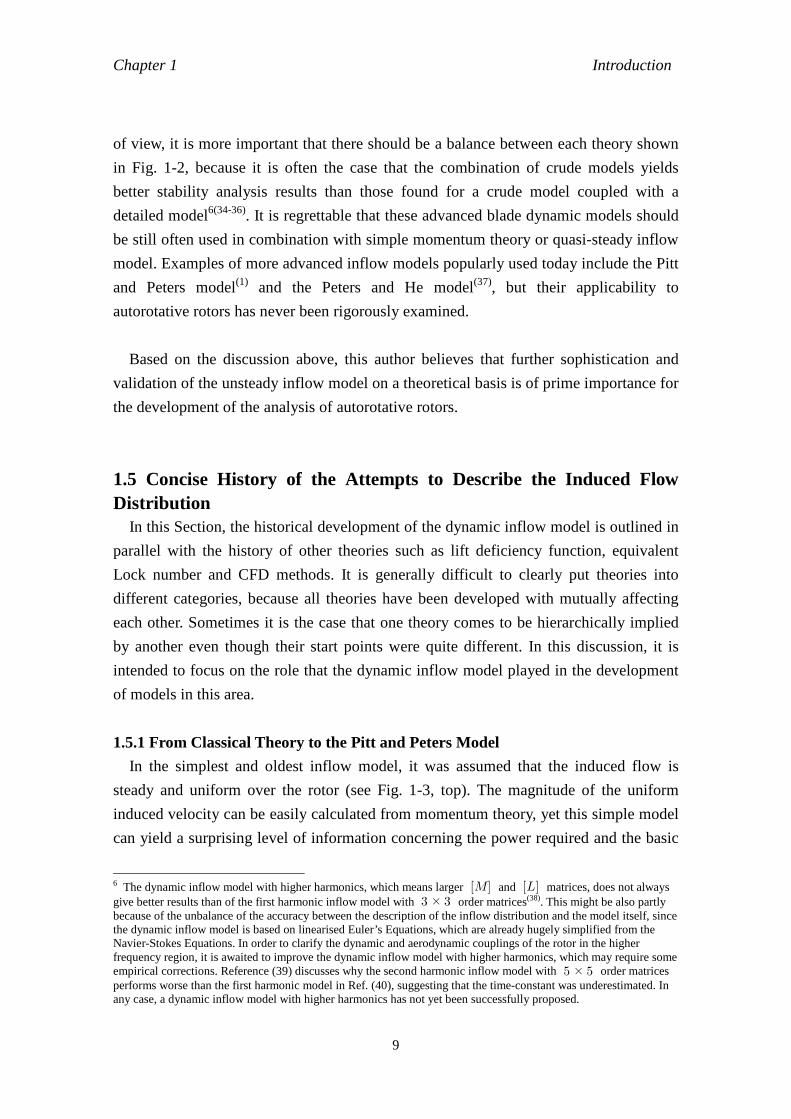
In the simplest and oldest inflow model, it was assumed that the induced flow is
steady and uniform over the rotor (see Fig. 1-3, top). The magnitude of the uniform
induced velocity can be easily calculated from momentum theory, yet this simple model
can yield a surprising level of information concerning the power required and the basic
6 The dynamic inflow model with higher harmonics, which means larger [M] and [L] matrices, does not always give better results than of the first harmonic inflow model with 3 3 order matrices(38). This might be also partly because of the unbalance of the accuracy between the description of the inflow distribution and the model itself, since the dynamic inflow model is based on linearised Euler’s Equations, which are already hugely simplified from the Navier-Stokes Equations. In order to clarify the dynamic and aerodynamic couplings of the rotor in the higher frequency region, it is awaited to improve the dynamic inflow model with higher harmonics, which may require some empirical corrections. Reference (39) discusses why the second harmonic inflow model with 5 5 order matrices performs worse than the first harmonic model in Ref. (40), suggesting that the time-constant was underestimated. In any case, a dynamic inflow model with higher harmonics has not yet been successfully proposed.
Chapter 1 Introduction
10
flight performance in hover(5). In the forward flight, however, the blades have different
relative airspeeds at different positions on the rotor, and the uniform distribution cannot
be realistically applied. Glauert proposed a linear distribution in which a longitudinal
gradient is considered(5,41).
Fig. 1-3 [Comparison between the uniform distribution and Glauert’s model.]
Glauert’s model is effectively a first order linear approximation, and is too simple to
provide an accurate representation for the complicated induced flow distribution found
in practice, but yields reasonable results when applied with an appropriate gradient. The
induced flow field in Glauert’s model is described as follows,
v = v0(1 +KcR
rcos ψ), (1.4)
where Kc represents the longitudinal gradient of the distribution, and v , v0 , r, R and
ψ denote the (axial) induced velocity, the uniform induced velocity, radial position on
the rotor disc, the rotor radius and the rotor azimuth, respectively. (See Fig. 1-3,
bottom.) Many values were theoretically or experimentally proposed for Kc, and the
examples are found in Refs. (16) and (42). Coleman and Feingold(43) suggested
Kc = tan(1/2), and this was the first time that Kc had been represented as a function of
wake skew angle, 1. This was a marked improvement, because the distribution of the
induced velocity heavily depends on the wake skew angle. Stepniewski introduces in
Ref. (44) a broader variety of presupposed static distributions of the induced velocity.
Note that in momentum theory, the magnitude of induced velocity is evaluated
regardless of the number of blades, airfoil section, chord length, blade twist, planform,
rotor speed and so on. In order to include these detailed aspects of rotor, there was a
school of attempts starting from blade element theory to describe the induced velocity,
Chapter 1 Introduction
11
examples of which can be found in Refs. (44) and (45).
Harris and McVeigh assumed that the local angle of attack of a blade should be zero
at the root and tip so that the lift should be zero, which means that induced velocity
forms a zero relative angle of attack at these points even in forward flight(45). These
works based on blade element theory helped to promote the improvement in the theory
of non-uniform induced flow distribution. Harris further studied full-articulated rotors at
low advance ratios, which exhibit an excessive amount of lateral flapping, correlating
wind tunnel test data with several classical inflow theories and numerical simulations
based on the prescribed wake method(46). Harris concluded that none of those theories
were satisfactory in predicting the lateral flapping at low advance ratios. This result
indicated that an essential improvement in the theoretical models was still necessary.
The first attempt to rigorously describe the distribution in a theoretical manner in the
frame of actuator disc theory can be traced back to Kinner(47), who introduced the
ellipsoidal coordinate system to describe the induced flow, and represented the
distribution of lift in the form of a functional series of the associated Legendre functions.
Note that these works introduced above are related not to the unsteady inflow
distribution, but to the steady distribution of the induced flow.
After the Second World War, the heyday of gyroplanes had passed, and the helicopter
came to be a practical class of aerocraft. Some important works concerning the unsteady
induced velocity were done in the 1950’s in the context of helicopter flight mechanics.
NACA engineers found through rotor whirl-tower tests in the 1950’s that when
increasing the collective pitch rapidly, there arises an overshoot of thrust(15). The reason
for this is that the delay of the induced flow in reaction to the change in the collective
pitch leaves the local angle of attack high until the angle is decreased by the newly
developed induced velocity7 . This finding attracted the attention of rotorcraft
aerodynamicists at the time to unsteady phenomena of the induced flow.
Mangler and Squire conducted one of the most important studies considering the
7 One important aspect with this phenomenon is that the airfoil may generate lift at a higher angle of attack than its stall angle, because there is also a delay in the occurrence of stall. As a result, the overshoot of thrust sometimes can be as large as double the maximum lift in the steady state. This phenomenon is called dynamic stall. Examples of such radical overshoot of thrust include a rapid yaw control of helicopters, and this led to the possibility of serious damage in the tail rotor because the overshoot of tail rotor thrust surpasses the maximum steady state value, upon which the structure was designed. The induced velocity delayed in the response is now called dynamic inflow and this is the root of the name of the dynamic inflow model(15).
Chapter 1 Introduction
12
modelling of an unsteady distribution of the induced flow undertaken in this period(48).
They first associated Kinner’s distribution of lift, which satisfies Laplace’s equation and
can describe the pressure discontinuity across the rotor, with the induced velocity field
in the form of Euler’s Equations. In their model, the rotor is treated as a solid circular
disc as in actuator disc theory, and a lift distribution is assumed so as to satisfy the
desired hub load. Mangler and Squire’s model can be regarded as the theoretical
archetype of the dynamic inflow model in the sense that the acceleration of the induced
flow was therein implied. However, the method of coupling the rotor load with induced
velocity was not as sophisticated as that of modern dynamic inflow models8. Joglker
and Loewy extended Mangler and Squire’s theory to incorporate the wake geometry(49)9.
Carpenter and Friedvich(50) presented another important work that also took the
dynamic inflow effect into consideration, motivated by the “jump take-off” of
overloaded helicopters. Some gyroplanes in the 1930’s already practised jump take-off,
which is a vertical take-off achieved by suddenly increasing the collective pitch of the
rotor, which is sufficiently prerotated at the minimum collective pitch. Jump take-off is
often explained as a sudden conversion of the excess kinetic energy stored in the rotor
into the rotor work, but the overshoot of thrust due to the dynamic inflow effect is also
important. Unfortunately, the dynamic inflow effect was not well understood by
gyroplane engineers at that time. Carpenter and Friedvich’s approach was quite different
from Mangler’s; they simply extended momentum theory by adding an extra term,
apparent mass term, which accounts for the delay in the induced flow to respond to
changes in collective pitch. Their model is now called unsteady momentum theory. The
remaining problem therewith is how to evaluate the apparent mass, and they adopted the
value of 8/32 ≃ 63.7 % of the air mass in a sphere with the same diameter as the rotor,
following Ref. (51). Their unsteady momentum theory can be simultaneously coupled
with other equations about blade dynamics, and the computed results agreed well with
experimental data for hovering flight.
Whereas the phenomenon caused by the dynamic inflow have been increasingly
attracting the interest of helicopter aerodynamicists since the 1950’s, most of the efforts
in modelling the induced velocity distribution was still focused on the static distribution,
in part because more basic information about the inflow distribution was first required 8 Reference (57) shows that Mangler and Squire’s model does not agree well with experimental data. See also Ref. (28) about the accuracy of the model. 9 Although the whole picture of their model is highly complicated, one particularly instructive feature of Ref. (49) is that it presents a lucid and detailed rearrangement of the equations for aerodynamic coefficients expressed in ellipsoidal coordinates, which are seldom provided in other literature.
Chapter 1 Introduction
13
at that time(52-54).
In the meantime, Sissingh developed a new model in which the roll and pitch
coupling of a rotor and their damping effect were linked with the variation of the
dynamic inflow(55). This cross-coupled damping effect was first reported in Ref. (56),
but was not well explained by the existing theories in which a uniform distribution of
the induced velocity was assumed. Sissingh assumed non-uniform distribution of the
induced velocity, and associated the variation with the first harmonic variation of the lift
coefficient. The idea of explaining the cross-coupled damping effect by non-uniform
inflow variation was novel, and led to the contemporary dynamic inflow model, Eq.
(1.3). Sissingh’s results agreed with the experimental data of Amer so well that his
approach was adopted in Lockheed REXOR Program and McDonnell-Douglas’
(formerly Hughes) simulation program FLYRT(29). However, Sissingh assumed that the
reaction of the inflow should occur instantaneously, and did not take the dynamic delay
into account. His model is therefore called quasi-steady model. Moreover, Sissingh
formulated the inflow distribution as a Fourier series dependent only on the azimuth,
but did not consider the radial variation.
Wheatley mentioned the close relation between the induced flow and the rotor load,
and the possible problems with noise and vibration(16) as early as in the 1930’s, but it
was not until the 1960’s that this relationship attracted more general attention, partly
because of the advent of hingeless rotor, which was first adopted in the
Messerschmidt-Bölkow BO105 in the late 1960’s by virtue of the development in
composite materials. The hingeless rotor is more sensitive to the variation of rotor load
than full-articulated rotors, and hence the inclusion of inflow distribution into the model
of the control system came to be considered as a vital necessity.
Curtiss and Shupe associated non-uniform rotor load with perturbations in pitching
and rolling moments for hingeless rotors in axial flight in the frame of a quasi-steady
model in 1971(58). Instead of fully incorporating dynamic inflow effects, they modified
the Lock number to account for the dynamic change in lift. Note that the reduced Lock
number10, which is usually called the equivalent Lock number, can be identified with
Loewy’s or Miller’s lift deficient function. Bannerjee et al. compared both the
equivalent Lock number method and the dynamic inflow model with experimental data,
10 The Lock number is defined as E = acR4/I . Reducing the Lock number is thus intuitively equivalent to assuming a heavier blade.
Chapter 1 Introduction
14
and concluded that the dynamic inflow model works better at low advance ratios up to
0.4(59).
The techniques of taking experimental measurements of the induced velocity
distributions have been developed since the 1960’s onwards, and examples include Refs.
(60) and (61). Gaonkar and Peters later described the situation, “... the theory of
dynamic inflow has been driven constantly by the impetus of experimental data.” in Ref.
(62). In point of fact, those experiments showed that unsteady momentum theory does
not agree sufficiently well with experimental data, and this became the trigger to further
develop the dynamic inflow model to cover forward flight conditions. Wood and
Hermes tried to combine momentum theory and blade element theory to describe the
induced flow in forward flight(63), and Azuma and Kawachi proposed the local
momentum theory, in which instantaneous momentum balance at a local blade element
is considered, and the blades are approximated as multiple wings, each of which has an
elliptical circulation distribution(64). The local momentum theory was so designed that
the time-wise decay of the induced flow can be described by an attenuation coefficient
even in unsteady forward flight.
In 1972, Ormiston developed the idea that the Fourier coefficients of the distributions
of induced velocity and lift should be associated in the form of a matrix equation. Since
he described the lift by circulation based on the Kutta-Joukowski theorem and blade
flapping dynamics was also incorporated, the model resulted in an elaborate
formulation(27). The representation of induced velocity was not therein completed
because only the time-averaged velocity distribution was considered in the model, and
thus, as Ormiston himself stated in the paper, the major significance of the work should
be in the mathematical rigour in the derivation.
Ormiston also developed a quasi-steady model with Peters to show that inclusion of
the non-uniform distribution of the induced velocity of a hingeless rotor improved the
agreement between the theory and experimental data(65). Although their model was still
partly based on complicated circulation theory, it was more accessible than the previous
model in Ref. (27), and the correlation with experimental data was significantly
improved. However, some elements of the gain matrices for this model were constant
regardless of the wake skew angle or any other flight variables, and some non-diagonal
terms are assumed to be zero, that is to say, cross-coupling effects are not sufficiently
taken into consideration.
Chapter 1 Introduction
15
Peters further developed the model to the form of Eq. (1.3) including the apparent
mass matrix(66), and demonstrated that the unsteady non-uniform induced velocity and
the blade aeroelasticity have a significant effect on the response characteristics of the
rotor system. However, the model is only appropriate for hovering flight, and thus the
non-diagonal elements of the gain matrix were not therein considered. Moreover, the
elements of matrices were not mathematically rigorously determined.
In 1976, Ormiston proposed an advanced mathematical model in which flapping
angle, inflow components and pitch angle are expanded as a Fourier series, and the
flapping angle and inflow components are unified in the form of a matrix equation,
which is suitable for eigenvalue analysis(67). Although only the first harmonics (i.e.
longitudinal and lateral components) are therein considered, off-diagonal elements of
matrices are also provided, and thus some cross-coupling behaviour of the rotor is also
taken into account. The formulation is an important milestone towards the contemporary
dynamic inflow models.
Various attempts at establishing the dynamic inflow model were made by many
researchers at this time in rather a parallel manner, and the examples include Refs. (68),
(69) and (70). White and Black’s model(69) is quasi-steady, and Johnson’s model(70) is
similar to Carpenter and Friedvich’s unsteady momentum theory. Although all of these
references concluded that their models showed a considerable progress in correlation
with experimental data such as Ref. (62), none of them could satisfactorily fully explain
dynamic inflow effects. Crew, Hohenemser and Ormiston tried to formulate the
reduction in control hub moment due to dynamic inflow effect in hover by either using
the equivalent Lock number method or replacing the inflow term in the blade equations
with an equivalent inflow term. Reference (71) has a brief summary of some of those
various dynamic inflow models presented in this period. (Note that it is pointed out in
Ref. (29) that the summary of Ref. (71) contains a misconception that the lateral and
longitudinal components of the induced flow, ?1s and ?1c , are missed in the
time-derivative part, i.e. the vector multiplied by the apparent mass matrix, resulting in
an erroneous expression for the uniform component of induced velocity.)
Another important study of this period was conducted by Peters and Gaonkar(72).
These authors extended the equivalent Lock number approach(59), which was used in the
frame of quasi-steady model for studying flapping stability, to the advanced dynamic
inflow model for studying flap-lag stability. They conducted extensive calculations for
Chapter 1 Introduction
16
the following model types: no induced flow perturbations, quasi-steady momentum
theory, unsteady momentum theory, an empirical model and the equivalent Lock
number model. They concluded that the dynamic inflow effect significantly increases
the flap-damping, and reduces the lag-damping. Some experimental attempts were also
made to identify the elements of the gain matrix(73). Gaonkar et al. studied the dynamic
inflow effects on the flap-lag stability with a quasi-steady model using the equivalent
Lock number(74).
The study of Van Holten, Ref. (75), is an important example of three-dimensional
unsteady rotor modelling based on acceleration potential theory. This study cast a doubt
on whether the classical lifting line model is valid for unsteady rotor dynamics, and
represented the (incompressible) induced flow field in the form of asymptotic
expansions. The theoretical basis and the limitation of Van Holten’s model are examined
in Ref. (76). Although Van Holten’s model is mathematically rigorously derived, the
model is represented in the form of integral equations, and is not well suited for flight
dynamics applications.
The most important achievement in the history of dynamic inflow model was
arguably made by Pitt and Peters(1), who extended the model of Ref. (65) for hovering
to fully include forward flight. The characteristic features of this model are its versatility,
possibly wide applications, the convenience it offers in being able to be used for
stability and control analysis, and the quite mathematical presentation of its derivation.
The equivalent Lock number approach is therein completely abandoned, and the gain
matrix is described as a function of the wake skew angle. In Ref. (28), Chen presents
intensive comparisons between the Pitt and Peters model and other dynamic inflow
models including those models proposed in Refs. (43), (69) and (77). Chen concluded
that the Pitt and Peters model shows an overall better agreement with experimental data
than other models. Reference (78) introduces the derivation of the Pitt and Peters model
in detail, together with an extensive literature review and comparison with other
numerical models.
1.5.2 Lift Deficiency Function
Whether steady or unsteady, the idea of associating the induced velocity with rotor
loads can be considered essentially based on simple Newtonian mechanics. On the other
hand, there is a different approach, in which the distribution of induced flow is
calculated from the distribution of vortices through the Biot-Savart law. The lift
Chapter 1 Introduction
17
distribution is also associated with the vortex distribution by means of the
Kutta-Joukowski theorem. This approach generally becomes much more
computationally intensive than the dynamic inflow model, but is more suitable for
studying the detailed shape and behaviour of the rotor wake and for incorporating
detailed blade geometry11. Moreover, the vortex method is suitable for studying
unsteady aerodynamics by considering the interaction between unsteady vortices.
The study of unsteady rotor aerodynamics using the vortex method may be traced
back to Glauert(79). Theodorsen developed the study and introduced Theodorsen’s lift
deficiency function, C(k), to account for the loss in circular lift due to the dynamic
development of the wake of an oscillating blade(80). Reference (5) presents the detailed
mathematical derivation of the lift deficient function. Theodorsen’s work was really a
milestone in theoretical unsteady aerodynamics, yet the distribution of the induced flow
is in reality much more complicated than what Theodorsen presumed, and thus the
approach needed further sophistication. References about the development of lift
deficiency functions include Refs. (81), (82) and (83). Greenberg coupled Theodorsen’
lift deficiency function with the quasi-steady model. Willmer regarded the trailing wake
from the outer part of a blade straight by neglecting its curvature, and succeeded in
representing the azimuthal variation of lift, which showed a reasonable agreement with
experimental data.
Miller introduced the concepts of the near wake and far wake, and concluded that the
higher harmonic rotor loads are evident during forward flight and are subject to the far
wake, and also that the higher harmonic loads are sensitive to the vertical spacing of the
wake sheet layers(85). Loewy improved Theodorsen’s lift deficiency function by
incorporating the spacing function to account for the influence of the shed vorticity, and
this modification made the lift deficiency function much more useful in rotorcraft
analysis. Loewy’s work reconfirmed not only the importance of three-dimensional
modelling of the rotor wake for rotorcraft analysis, but also the necessity of taking the
dynamic inflow effect into consideration when studying critical flutter speed and so
on(86). Loewy’s function is a great improvement from Theodorsen’s though, only
11 As is discussed in Section 1.3, the dynamic inflow model is based on simple actuator disc theory. Although the dynamic inflow model is highly flexible to combine with any other advanced blade dynamics theories(7,36), the start point (i.e. actuator disc theory) can be an inherent limitation of the approach. On the contrary, the vortex method is able to incorporate elaborate blade geometry and dynamics from the beginning, and can impart more intricate distribution. However, its minuteness sometimes leads to a lack of versatility, and the computational intensity may also be a problem. It should be noted here that these two theories are not incompatible, and can indeed be used in conjunction to overcome either of the single method’s shortcomings. One example of such an attempt is found in Ref. (84).
Chapter 1 Introduction
18
two-dimensional vortex sheets are therein assumed, and hence the limitation of this
assumption leads to the following shortcomings, which are pointed out by Peters and
He(7): (i) skewed helical vortex geometry, which is expected in forward flight, cannot be
incorporated; (ii) the model has a singularity for the collective mode at the zero
frequency, and the model is thus not suitable for low frequency problems; (iii) the
theory is based on the frequency domain, and the applications coupled with other
theories such as eigenvalue analysis flight dynamics are limited; and (iv) the model is
not suitable to utilize for control systems.
Some attempts to improve Loewy’s lift deficiency function include Refs. (87), (88)
and (89). Jones and Rao(87) developed Loewy’s lift deficiency function so as to
incorporate the compressibility of air using the acceleration potential. Taking the
compressibility of air into account was quite novel since most of precedent models
presupposed only incompressible flow at that time. However, Jones and Rao did not
consider time delay in the response of the air, and thus their model was also a
quasi-steady model. This approach has the problem that compressible air needs some
time to transmit a signal, and thus such a quasi-steady modelling should be valid only
for incompressible flow.
Hammond and Pierce(88) improved Jones and Rao’s model by incorporating the
time-delay in the response of induced velocity. Friedmann and Venkatesen(89) modified
Loewy’s lift deficiency function in conjugation of quasi-steady inflow model of
Greenberg(82), perturbation inflow model(71) or dynamic inflow models of Johnson(70),
and studied the stability of the fuselage/rotor coupling dynamics in ground resonance. It
is interesting that the final forms of these models, which are based on lift deficiency
function, came quite close to the dynamic inflow model, which was introduced in the
previous section, despite these models were developed from quite different start points.
The concept of lift deficiency function was originally simply a correction function
based on two-dimensional wake theory and was defined in frequency domain, but
Friedmann and Venkatesen converted the representation into time domain using
classical control theory, in which Loewy’s lift deficiency function is recognized as a
transfer function relating the 3/4-chord induced velocity to the lift of the reference blade.
This mathematical sophistication associates Loewy’s lift deficiency function with the
two-dimensional dynamic inflow model in the finite state form, and the contribution
thereof to two-dimensional unsteady aerodynamics is both theoretically and practically
Chapter 1 Introduction
19
of great importance(90,91). Friedmann and Venkatesen finally proposed a dynamic inflow
model of the same form as Eq. (1.3)(90), which was developed from Loewy’s lift
deficiency function. Reference (92) gives a lucid explanation how classical lift
deficiency functions can be hierarchically implied by more advanced dynamic inflow
models.
1.5.3 Computational Method
Since there are a number of technical references published regarding various
computational methods, which are most rapidly developing tools in this field, it should
be out of scope of this thesis to introduce all their details. Instead, only characteristic
features of computational methods shall be herein introduced in comparison with
dynamic inflow models.
In Theodorsen’s lift deficiency function theory, considerable simplifications and
assumptions such as a two-dimensional wake sheet and constant vertical spacing
between wake sheets are introduced. This was inevitable at that time in part because
computers of the time were not able to track the complicated behaviour of vortices,
which affect each other by their own induced velocity fields. Nowadays, owing to the
rapid development in the computational technology, much more computationally
intensive calculations can be conducted with smaller number of assumptions or
simplifications at a much lower cost. These computational methods based on the vortex
theory and the Biot-Savart law can be classified roughly into three types: (i) rigid wake
model, (ii) prescribed wake model and (iii) free wake model. A rigid wake is assumed in
the rigid wake model, and this is the strongest assumption, which in turn corresponds to
the lightest computational load. In a prescribed wake model, the distribution of vortices
is either empirically or semi-empirically prescribed at the initial state, and then the
development of the wake distribution is computed through the Biot-Savart law. The free
wake model is the most computationally intensive, and allows the wake distribution
develop freely. Owing to the rapid development in computational resources, the free
wake method is increasingly used and became the mainstream of contemporary CFD
methods. The basic ideas of these methods are lucidly explained in Ref. (5), and the
reader may refer to Refs. (77), (85), (93), (94) and (95) for further details concerning the
historical development of these computational methods.
One characteristic feature of these computational methods, especially with free wake
method, is that simulations of the development of the rotor wake can be conducted
Chapter 1 Introduction
20
based only on the first principles such as the Navier-Stokes equations, Biot-Savart law
and vorticity transport equation(5) 12. Recent rapid development in computational
resources has made it possible to mesh the pertinent flow field and solid boundary
(blades, hub, etc.) into millions of cells, and to simulate the resultant distortion in the
three-dimensional wake distribution and the induced flow field in the time domain. The
advantages of free wake analysis include the detailed description of the complicated
flow field, the local treatment of airfoil dynamics, a thorough inclusion of complex
interaction of vortices and specific boundary conditions, and the relatively low cost of
conducting computations compared to full-scale experiments. Since the inflow is only
globally treated in the dynamic inflow model, the detailed description from vortex
methods is clearly better suited to examining locally complicated aerodynamic
phenomena. Regarding the degree of reality of the wake description, it can be said that
momentum theory is too simple, CFD methods are most convoluted, and the dynamic
inflow method lies between these other two. Thus, momentum theory is most suitable
for evaluating basic performance of rotor, CFD methods are for complicated local
aerodynamic phenomena, while the dynamic inflow model is for analysing general
stability (frequency, damping, modal information, etc.), control characteristics, vibration,
handling qualities and transitional rotor dynamics13.
A disadvantage of the CFD approach is that those vortex methods are not suitable for
eigenvalue stability analysis because of the large number of states required to describe
the unsteady wake. Another shortcoming in CFD simulations is that only the most stable
state is presented in the simulation even when there are a plural of bifurcated non-linear
solutions to the governing non-linear equations. Since the Navier-Stokes equations and
the Euler equations are non-linear, they may give either non-linear solutions, which
bifurcate from linear or other non-linear solutions, or isolated non-linear solutions,
which do not bifurcate from any other solutions. These hidden secondary or tertiary
solutions are usually neglected in numerical simulations because the most feasible
solution is trailed step by step from the primary linear solution in a time-marching
simulation, but, in fact, non-linear jump can happen in reality, i.e., it is possible that the
physical state can change to an isolated state(97). Furthermore, eigenvalue stability
12 Roughly speaking, a vortex is generated around a solid boundary, transported according to the induced flow, which other vortices induced, and vanish due to the viscosity of the fluid. 13 Padfield suggested three levels of methods of rotorcraft simulation models in Ref. (96): in Level 1, the induced flow is described as a superposition of a finite number of simple flow states on the disc as a first-order model; in Level 2, the disc is replaced by individual blades; in Level 3, the entire rotor wake geometry is taken into consideration. According these three levels, it can be said that the momentum theory and advanced CFD methods correspond to the level 1 and 3, respectively, and the dynamic inflow model is supposed to cover more or less the level 2.
Chapter 1 Introduction
21
analysis is necessary in order to find bifurcated non-linear solutions. The free wake
method is thus not suitable for stability analysis of non-linear solutions. Whereas
dynamic inflow models are linear in general, they offer a greater flexibility to be
combined with non-linear theories, and the examples include the study of Bassett(98), in
which the Peters and He model(37) is used14. Houston and Brown showed a unique
attempt to compare the dynamic inflow model with a vortex transport wake model
focused on flight mechanics in autorotation(99), and concluded that the dynamic inflow
model works satisfactorily for much of the autorotation regime except for steep descents,
in which a comprehensive description of the inflow is essential.
1.5.4 From the Pitt and Peters Model to the State of the Art
The Pitt and Peters model is a significant milestone in the history of rotorcraft
aerodynamics. It was the first truly practical dynamic inflow model which could be used
for control system analysis, and well agreed with experimental data both for hovering
and forward flight(28,100). Dynamic inflow effects are so important in control and
stability analysis that a convenient and versatile dynamic inflow model such as the Pitt
and Peters model had been long-awaited. Nagabhushanam and Gaonkar(101) studied air
resonance stability in forward flight by both the three-state and five-state models of Pitt
and Peters. The torsional flexibility of the blades is also therein considered, and the
stabilities of various modes are extensively examined. They concluded: the three-state
model is more consistent than the five-state model in general; dynamic inflow tends to
increase stability margins in general, that the air resonance characteristics are
independent of the number of blades; and appropriate combination of aeroelastic
coupling parameters can significantly improve air resonance stability. Reference (62)
(or Ref. (102), which is almost identical to Ref. (62)) shows how dynamic inflow
models were developed due to the desire to correlate with experimental data15, and
14 The dynamic inflow model is more suitable for stability analysis of non-linear solutions(98,103), though non-linear analysis in this field still awaits further development. Poiseille flow in a circular pipe is maybe an example of non-linear jump. No non-linear solutions bifurcated from the linear solution are hitherto found analytically, and the linear solution is analytically proven to be absolutely stable. However, as the Reynolds number increases, the flow changes from laminar to turbulent flow. This is considered to be a non-linear jump from the linear solution to an isolated non-linear solution, though any isolated solutions have yet been analytically found. Generally speaking, a turbulent flow may in practice be described by an orbit in phase space between two or more unstable equilibrium solutions to the governing equations, where these unstable equilibrium solutions cannot be found by simulation approaches. 15 These authors concluded that the Pitt and Peters model agrees with experimental data quite well in hover. However, their correlations in forward flight or transient flight cases are poor, conceivably because of the lack of experimental data for these flight cases. The accuracy of Pitt and Peters model, which is at least as accurate as momentum theory, is predictable in hover because the model hierarchically implies momentum theory. The novel aspect with the Pitt and Peters model is the continuous representation of the gain matrix from axial to edgewise flight cases, and some further comparisons with experimental results to the model’s performance for these cases is desirable. This author shall examine the Pitt and Peters model in Section 2.3.
Chapter 1 Introduction
22
presents a comparison between the results obtained from the Pitt and Peter model with
experimental data including Ref. (61).
Dynamic inflow effects are of great importance in rotor stability analysis because
dynamic inflow modes have nearly the same order of magnitude as those of flapping or
lead-lag modes, and significantly affects the stability of various blade motions or
aeromechanical phenomena such as ground resonance, air resonance, blade flapping,
rotor-body coupling, pitch-roll coupling, flap-lag coupling and so on. Chen and Hindson
extensively studied dynamic inflow effects on the stability in the vertical acceleration
response of the helicopter in both the Carpenter and Friedvich model and the Pitt and
Peters model with various thrust coefficients and blade Lock numbers. This study was
conducted with the purpose of developing a super-augmented high-gain flight control
system for military helicopters(104). These authors reconfirmed the importance of
dynamic inflow effects in control and stability analysis, reporting that both models
performed well in comparison with NASA flight test results from CH-47B.
Although the Pitt and Peters model is widely used even now, it has the following
weaknesses:
i. hub loads are therein used as the aerodynamic load on the rotor to associate with the
induced velocity, that is to say, the model does not distinguish between different lift
distributions that yield the same hub loads. However, a model that can distinguish
specific lift distribution is required for blade structural analysis and aeroelastic
analysis;
ii. the Pitt and Peters model is based on simple actuator disc theory, even though it is
flexible enough to be coupled with more complicated blade element theory. This may
reflect an inherent limitation of the model to account for the more complicated
phenomena which are related to detailed blade geometry;
iii. the Pitt and Peters model is expressed in the perturbation form, but it is preferable for
practical purposes that variable are described in terms of the overall variables;
iv. variables in the Pitt and Peters model are defined in the rotor coordinates, but for
flight dynamics it would be more convenient to define the model in wind-axis
coordinates.
Pitt and Peters themselves re-examined their model critically inspecting the
assumptions such as actuator disc theory and the linearity of the distribution in
Chapter 1 Introduction
23
comparison with other inflow models(105,106). In Ref. (40), Gaonkar and Peters defined
the dynamic inflow effects as low frequency properties of the unsteady wake in contrast
to conventional high frequency airfoil dynamics such as flutter, and showed a
hierarchical relation between thirteen inflow models including quasi-steady, momentum
theory, the equivalent Lock number approach and full unsteady models of 3DOF and
5DOF. This thorough comparison is highly instructive, and the authors remarked that
there was no satisfactory replacement for momentum theory before the Pitt and Peters
model appeared. They concluded that quasi-steady modelling is sufficient at high
advance ratios, but that the dynamic inflow model of 5DOF is inadequate for a rotor
having fewer than 5 blades, and that 3DOF model is overall more accurate than the
5DOF model. Results of this work indicate to what extent the dynamic inflow model
needs to be sophisticated depending on the nature of individual problems. Regarding
points (iii) and (iv) above, Peters and HaQuang proposed a non-linear version of Pitt
and Peters model, in which all variables are treated not as perturbations but as in total
amount(107), expressed in the wind-axis coordinate system.
The non-linear version was adopted in NASA Ames helicopter mathematical model,
designated ARMCOP, and reportedly performed well(108). Gaonkar and Peters
summarised the historical development of the dynamic inflow model in Ref. (29), and
showed an intensive comparison between various models. This review is also extremely
instructive that it points out some misconceptions found in the past literature including
Refs. (65), (71), (89), (105) and (106), and also limitations to the applicability of either
the linear or non-linear dynamic inflow model.
The most important work which appeared after the Pitt and Peters model is arguably
the Peters and He model(7), which forms the theoretical basis of this thesis. The
derivation of this model is the most mathematically rigorous, and is consistent from the
first principles compared to its preceding models. A concise version of the derivation is
found in Ref. (37), and the model’s validation and correlation with experimental data
are shown in many research works, for example, in Refs. (30), (92), (109), (110), (111),
(112) and (113). In the Peters and He model, the representations of both inflow and
pressure distributions are generalised so that an arbitrary number of harmonics and
radial shape functions can be used for each state.
Reference (92) presents a comparison between the Peters and He model and the
experimental data from Refs. (114) - (116) using both rectangular and tapered blades,
Chapter 1 Introduction
24
and concluded that the model performs as well as or better than some computational
codes of free-wake and prescribed-wake methods at a smaller computational cost.
Reference (112) also compares the Peters and He model with classical theories and
computational methods with contrasting their shortcomings, and demonstrates that the
Peters and He model implicitly includes classical theories including Theodorsen’s and
Loewy’s lift deficiency functions and Prandtl-Goldstein’s tip-loss formula16. Reference
(39) is a notably instructive study, since it compares the Peters and He model with
various classical theories including Theodorsen’s, Loewy’s or Miller’s lift deficiency
functions and other finite-state methods. Reference (39) concluded that the Peters and
He model is overall superior to classical unsteady models, but it cannot provide an
accurate description of inflow in the close vicinity of the blade surface, nor can it
account for wake roll-up. The Peters and He model has been further improved in some
variations, with examples including Refs. (117) and (118), in which the ground effect is
incorporated. The ground effect in this modelling is described as an extra term in the
pressure potential in order to satisfy the boundary condition.
In applying the dynamic inflow model to a flight simulation code, there has been a
mystery that the simulated results sometimes predict a completely opposite off-axis
response in hover and low speed forward flight in comparison with the corresponding
flight test data(119-123). A large number of publications related thereto suggested many
possible causes for this phenomenon including gyroscopic force of the wake(124),
aerodynamic interaction between the rotor and fuselage(125), dynamic twisting of the
blade(126), wake distortion(127,128) and so on. It is highly likely that several of these
mechanics are therein coupled in a complex manner. This problem is an active area of
current research. Regarding the wake distortion, Ref. (129) proposes that the gain
matrix in the Peters and He model should be modified as an augmented L-matrix so as
to account for the effects due to wake curvature in non-hover flight conditions. Those
models which have augmented gain matrix are called the augmented Peters and He
model or augmented Pitt and Peters model, depending on the base model, and the
literature about these augmented models includes Refs. (130) - (134). Note that the
complicated wake distortion effects are incorporated in these models by wake curvature
parameter, KR , which is empirically determined. Reference (134) introduced the
augmented Pitt and Peters model in which wake skew, wake curvature and wake
spacing are incorporated as additional states in transitional flight.
16 It may be rather odd that Pitt and Peters model is not compared with the Peters and He model at all either in Ref. (92) or (112) in spite of comparisons with many of more classical theories. This author will present his own view about the Pitt & Peters and Peters & He models in Section 2.3.
Chapter 1 Introduction
25
Zhao(135) presented a table of various values of KR for comparison, and proposed
augmented models for both the Pitt & Peters and Peters & He models including detailed
mathematical derivations. In Ref. (135), a more refined description of the wake
curvature which is expressed by lateral and longitudinal wake curvatures, Kc and Ks,
is also proposed. The inclusion of the wake effects into dynamic inflow modelling is
still an up-to-date issue in the field, and further improvement, validation and correlation
with experimental and CFD simulation data are required, partly because the correction
parameters must be essentially empirically determined.
References (136) and (137) propose a state-of-the-art methodology whose
mathematical derivation is quite different from that of the Peters and He model. The
model is based on the conservation equations of mass and momentum, and they are
transformed into state-space forms by the Galerkin method so that the Peters and He
model is therein hierarchically implied. A velocity potential is also therein considered
on top of an acceleration potential, and both off- and on-disc flow are described by the
set of three components. Although it seems that the Peters and Morillo model has not
yet been widely utilized at present, it will likely be the leading next generation dynamic
inflow model.
1.6 Literature on Autorotation In this Section, the historical and current state of works on gyroplanes and helicopters
in the windmill-brake state is briefly introduced in order to outline the importance of
this research in the relevant context. Cierva himself made a huge contribution to the
development in the theory of early gyroplanes from both theoretical and practical points
of view(2,3,4,138). (The left picture of Fig. 1-4 is Cierva’s Type C.4, which made the first
controlled gyroplane flight in 1923.) British aerodynamicists such as Lock and Glauert,
whom Cierva vehemently criticised, made more rigorous theoretical
work(20-22,41,79,139-143). Concurrently, a number of experimental and theoretical studies
were intensively conducted in the U.S.A. by NACA engineers such as Wheatley and
others(16-19). Indeed, there was a sound basis for further studying the characteristics and
aerodynamics of the gyroplane at that time. The initial development in the Autogiro by
Cierva is introduced in Ref. (144) in rather a story-telling manner, while Ref. (145)
gives detailed background about the gyroplane both in historical and technical aspects.
Despite the great success of gyroplanes in commercial and military fields in the 1930’s,
the mainstream of rotorcraft research shifted to the helicopter after the 1940’s. Most of
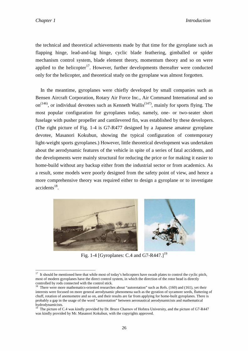
Chapter 1 Introduction
26
the technical and theoretical achievements made by that time for the gyroplane such as
flapping hinge, lead-and-lag hinge, cyclic blade feathering, gimballed or spider
mechanism control system, blade element theory, momentum theory and so on were
applied to the helicopter17. However, further developments thereafter were conducted
only for the helicopter, and theoretical study on the gyroplane was almost forgotten.
In the meantime, gyroplanes were chiefly developed by small companies such as
Bensen Aircraft Corporation, Rotary Air Force Inc., Air Command International and so
on(146), or individual devotees such as Kenneth Wallis(147), mainly for sports flying. The
most popular configuration for gyroplanes today, namely, one- or two-seater short
fuselage with pusher propeller and cantilevered fin, was established by these developers.
(The right picture of Fig. 1-4 is G7-R477 designed by a Japanese amateur gyroplane
devotee, Masanori Kokubun, showing the typical configuration of contemporary
light-weight sports gyroplanes.) However, little theoretical development was undertaken
about the aerodynamic features of the vehicle in spite of a series of fatal accidents, and
the developments were mainly structural for reducing the price or for making it easier to
home-build without any backup either from the industrial sector or from academics. As
a result, some models were poorly designed from the safety point of view, and hence a
more comprehensive theory was required either to design a gyroplane or to investigate
accidents18.
Fig. 1-4 [Gyroplanes: C.4 and G7-R447.]19
17 It should be mentioned here that while most of today’s helicopters have swash plates to control the cyclic pitch, most of modern gyroplanes have the direct control system, in which the direction of the rotor head is directly controlled by rods connected with the control stick. 18 There were more mathematics-oriented researches about “autorotation” such as Refs. (160) and (161), yet their interests were focused on more general aerodynamic phenomena such as the gyration of sycamore seeds, fluttering of chuff, rotation of anemometre and so on, and their results are far from applying for home-built gyroplanes. There is probably a gap in the usage of the word “autorotation” between aeronautical aerodynamicists and mathematical hydrodynamicists. 19 The picture of C.4 was kindly provided by Dr. Bruce Charnov of Hofstra University, and the picture of G7-R447 was kindly provided by Mr. Masanori Kokubun, with the copyrights approved.
Chapter 1 Introduction
27
As mentioned in Section 1.2, it was the first time after the Second World War that
gyroplanes have been extensively investigated20 at the University of Glasgow as part of
CAA funded research programme following several grievous accidents in the United
Kingdom(148). The research topics include aerodynamic characteristics of various
configurations(8), qualitative or quantitative control and stability analysis(149,150),
rotorcraft flight dynamics in autorotation(9,10) and numerical simulation of autorotative
flight(151-153). Spathopoulos studied a mathematical model to simulate rotorcraft in
autorotation(154), and Bagiev assessed gyroplane handling qualities using both flight
tests and simulations(155). Some new projects to revive the gyroplane are presently under
way including a hybrid-gyroplane by Cartercopter(156), a turbine-powered gyroplane by
Groen Bros. Inc.(157) and some more conceptual designs such as massive VTOL
transport(157) and airbike(158). The possibility of using a gyroplane as unmanned
reconnaissance vehicle is also examined(159) in stability and dynamic characteristics21.
Academic studies of gyroplanes have thus recently restarted, and the future outcome
and scope of these projects are not yet clear.
The very first motivation of Cierva to invent the Autogiro was that he wanted to build
a safe vehicle which is free from stall. In fact, Ref. (144) reads about Autogiro, “...
although not designed with the sporting purpose of increasing speed not with the
commercial object of enlarging the radius of action, but with the humanitarian purpose
of reducing to a minimum the number of accidents and the number of human lives
sacrificed in the flight for the conquest of the air.” It is thus quite ironical that the
contemporary gyroplanes are designed chiefly for the sporting purpose, albeit not for
the speed, and hence are associated with unacceptable casualty rates. The flight
principle of the gyroplane itself is not in the wrong, and there still is a possibility that
the gyroplane can regain a prominent position in aviation if updated with state-of-the-art
advanced technology. What are urgently required now are further theoretical, practical
or experimental works such as mathematical models, technical knowledge, experimental
data and so on, to provide a sound technical basis either for improving contemporary
gyroplanes or for developing new gyroplanes.
20 In some projects of designing convertiplane, which is a mule of fixed-wing aircraft and rotarycraft, the flight principle of the gyroplane occasionally attracted some attention. These projects includes Fairy’s Rotordyne(162), whose concept is now tried to revive by Groen Brothers Inc.(157) There were also some attempts to develop a gyroplane for commercial purpose, but they all resulted in failure. 21 Interestingly, the authors concluded that the elevator control should be used together with longitudinal cyclic control, unlike the most of contemporary small gyroplanes, which usually have only small (or sometimes no) fixed horizontal stabilizer.
Chapter 2 Review of the Dynamic Inflow Model of Peters and He
28
Chapter 2
Review of the Dynamic Inflow Model of Peters and He
2.1 Introduction 2.1.1 Overview
In this Chapter, the theoretical derivation of Peters and He model will be reviewed in
depth and examined in detail. The general theory of dynamic inflow models has been
extensively developed by Peters and his coworkers in the last two decades, and the
Peters and He model is theoretically one of the most refined dynamic inflow models in
existence today.
The later Chapters of this thesis are based on the Peters and He model, and thus it is
necessary to first review the foundations of this model. As well as permitting the
foundations of the work of the present thesis to be presented, a review of this model is
also convenient since the relevant literature, including Refs. (1) and (7) offers a
somewhat disjointed view of the model’s derivation, which is not readily accessible. In
particular, some assumptions and theorems therein used are not explicitly declared or
proven in the original literature, and thus the present author tries to improve the lucidity
of the explanation of the mathematical derivation of this model by complementing the
details of some difficult rearrangements of equations and correcting some typographical
error contained in the original references. Although the author also presents new
explanations of some aspects of this derivation, it must be stressed here again that the
general idea of this Chapter is based on the works of previous authors, including Peters,
He and their coworkers. In particular, this Chapter is largely based on Ref. (7), which
should be the most thorough source of the pertinent theory. Some complementary
theorems and peripheral topics are discussed either in footnotes or appendices.
2.1.2 Notations
Symbols and notations are used so as to be as consistent with Refs. (1), (7) and (92)
as possible, although it should be noted that there is a variation of notations even
between these references. The author thus chose the most reasonable designations for
the case. Readers are encouraged to confirm the definitions when reading a plurality of
Chapter 2 Review of the Dynamic Inflow Model of Peters and He
29
literatures.
In this thesis, those variables that are related to the time-derivative and convection
terms of the Euler equation are denoted by (t) and (c) as superscripts, respectively. This
notation is original in this thesis, and it is hoped that it will facilitate a better
understanding. The variables that are related to Fourier coefficients for cosine and sine
functions are also given c and s as superscripts, respectively. For the Legendre functions,
r, j, i, k, m and n are used as dummy indices. No matter how confusing they may look,
the way of using letters in this Chapter is thus consistent. For example, Lrmcjn denotes a
Fourier coefficient having four indices of r,m, j and n, corresponding to a cosine
function.
2.2 Review of the Dynamic Inflow Model of Peters and He 2.2.1 Fundamental Assumptions for the Mathematical Derivation of the Peters and
He Model.
The Peters and He model is based on the following assumptions, (A1) - (A5):
(A1) the flow is inviscid. Thus, the induced flow is generated by the pressure
potential (or acceleration potential), and governed by the Euler equations,
∂t
∂U+ (U ∇)U = ∇Φ , (2.1)
where U, t and Φ represent non-dimensionalised velocity, time and a pressure
potential function, respectively22;
(A2) the pressure distribution over the rotor disc is continuous, but it has
a discontinuity across the rotor disc;
(A3) air flow is assumed to be incompressible and satisfies the equation of
continuity,
∇ U = 0 ; (2.2)
(A4) the rotor disc can be regarded as a flat orientable disc.
The assumption (A1) explains why the flow is not governed by the Navier-Stokes
equations, but by the Euler equations. Since the air flow around the rotor is sufficiently
fast (for example, a typical Reynolds number about a helicopter blade is 105 - 106), the
22 The Euler equations can be derived as a consequence of the conservation of momentum (Newton’s law of motion), if assumptions (A3) and (A1) are valid. Thus, assumptions (A2) and (A4) can mathematically be implied in assumption (A1) if Newtonian mechanics is approved. Although it may sound needless to state, assumption (A1) may be interpreted that Newtonian mechanics is considered to be valid.
Chapter 2 Review of the Dynamic Inflow Model of Peters and He
30
assumption (A1) can be reasonably used for most flight cases.
The assumptions (A2) and (A4) indicate that the model is based on actuator disc
theory, and the assumption (A4) gives the theoretical grounds for regarding the lift
working on the rotor disc as the pressure potential23. The assumption (A3) means that
air compressibility and shock wave effect are negligible. While this is not always the
case with high-speed helicopter flights, this assumption can still be reasonably valid for
a wide range of helicopter flights and for most gyroplane flights.
2.2.2. The Representation of the Pressure Field
The mathematical derivation of the dynamic inflow model essentially relies on the
principle of superposition of linear equations. Since Eq. (2.1) contains a non-linear term
(i.e. the convection term), which must be linearised in advance for dynamic inflow
modelling as follows (see also Appendix 2.1),
∂t
∂q (V ∇)q = ∇Φ , (2.3.1)
where V is the non-dimensionalised steady base flow, Φ is the pressure potential
which drives the induced flow and q is the induced flow, which is regarded as a
perturbation in this linearised equation. Note that the second term in the left-hand side
of Eq. (2.3.1) has a minus sign unlike Eq. (2.1), because positive q and V are defined
in opposite directions, as shall be seen in Fig. 2-2. In Cartesian coordinates, Eq. (2.3.1)
can be separated into the following three equations,
∂t
∂qx Vx∂x
∂qx Vy∂y
∂qx Vz∂z
∂qx= ∇xΦ , (2.3.2)
∂t
∂qy Vx∂x
∂qy Vy∂y
∂qy Vz∂z
∂qy= ∇yΦ , (2.3.3)
∂t
∂qz Vx∂x
∂qz Vy∂y
∂qz Vz∂z
∂qz= ∇zΦ . (2.3.4)
23 Note that the dynamic inflow model based on actuator disc theory can be subsequently coupled with any lift distribution, in which each blade shape may be considered in detail. Still, this should be considered as a combination of different theories, and it should be explicitly emphasised that the derivation of Peters and He model is based on simple actuator disc theory.
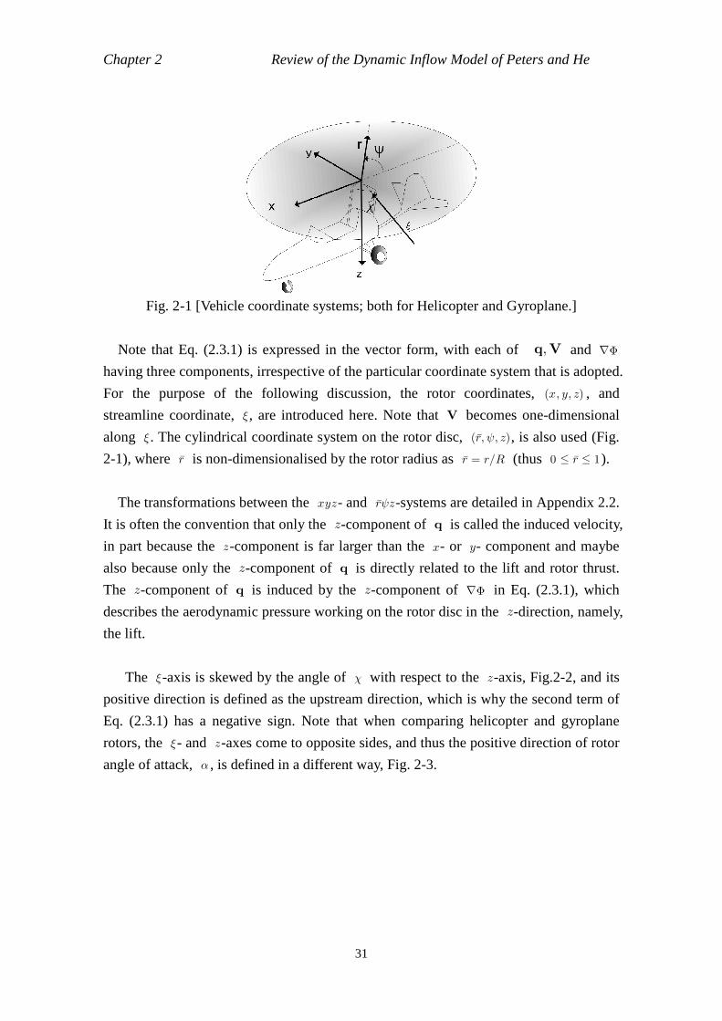
Chapter 2 Review of the Dynamic Inflow Model of Peters and He
31
Fig. 2-1 [Vehicle coordinate systems; both for Helicopter and Gyroplane.]
Note that Eq. (2.3.1) is expressed in the vector form, with each of q,V and ∇Φ
having three components, irrespective of the particular coordinate system that is adopted.
For the purpose of the following discussion, the rotor coordinates, (x, y, z) , and
streamline coordinate, $ , are introduced here. Note that V becomes one-dimensional
along $ . The cylindrical coordinate system on the rotor disc, (r, ψ, z), is also used (Fig.
2-1), where r is non-dimensionalised by the rotor radius as r= r/R (thus 0 r 1).
The transformations between the xyz- and rψz-systems are detailed in Appendix 2.2.
It is often the convention that only the z-component of q is called the induced velocity,
in part because the z-component is far larger than the x- or y- component and maybe
also because only the z-component of q is directly related to the lift and rotor thrust.
The z-component of q is induced by the z-component of ∇Φ in Eq. (2.3.1), which
describes the aerodynamic pressure working on the rotor disc in the z-direction, namely,
the lift.
The $-axis is skewed by the angle of 1 with respect to the z-axis, Fig.2-2, and its
positive direction is defined as the upstream direction, which is why the second term of
Eq. (2.3.1) has a negative sign. Note that when comparing helicopter and gyroplane
rotors, the $- and z-axes come to opposite sides, and thus the positive direction of rotor
angle of attack, : , is defined in a different way, Fig. 2-3.
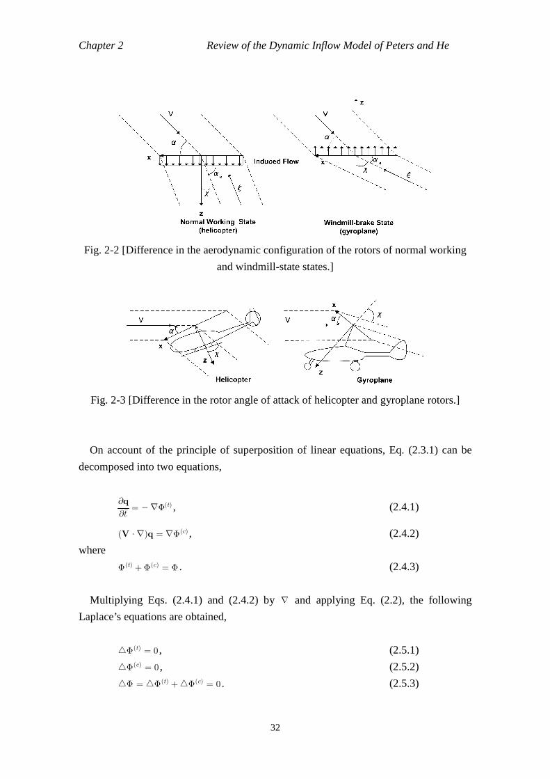
Chapter 2 Review of the Dynamic Inflow Model of Peters and He
32
Fig. 2-2 [Difference in the aerodynamic configuration of the rotors of normal working
and windmill-state states.]
Fig. 2-3 [Difference in the rotor angle of attack of helicopter and gyroplane rotors.]
On account of the principle of superposition of linear equations, Eq. (2.3.1) can be
decomposed into two equations,
∂t∂q
= ∇Φ(t) , (2.4.1)
(V ∇)q = ∇Φ(c) , (2.4.2)
where
Φ(t) +Φ(c) = Φ . (2.4.3)
Multiplying Eqs. (2.4.1) and (2.4.2) by ∇ and applying Eq. (2.2), the following
Laplace’s equations are obtained,
Φ(t) = 0 , (2.5.1)
Φ(c) = 0 , (2.5.2)
Φ = Φ(t) +Φ(c) = 0 . (2.5.3)
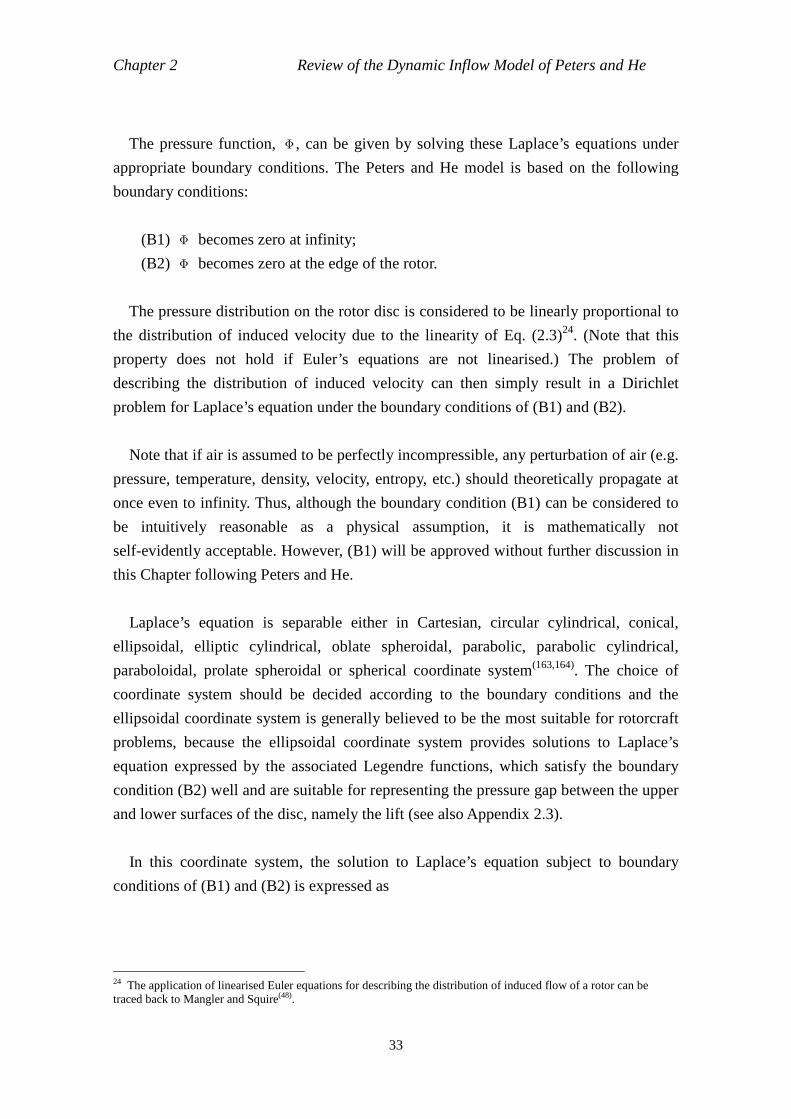
Chapter 2 Review of the Dynamic Inflow Model of Peters and He
33
The pressure function, Φ , can be given by solving these Laplace’s equations under
appropriate boundary conditions. The Peters and He model is based on the following
boundary conditions:
(B1) Φ becomes zero at infinity;
(B2) Φ becomes zero at the edge of the rotor.
The pressure distribution on the rotor disc is considered to be linearly proportional to
the distribution of induced velocity due to the linearity of Eq. (2.3)24. (Note that this
property does not hold if Euler’s equations are not linearised.) The problem of
describing the distribution of induced velocity can then simply result in a Dirichlet
problem for Laplace’s equation under the boundary conditions of (B1) and (B2).
Note that if air is assumed to be perfectly incompressible, any perturbation of air (e.g.
pressure, temperature, density, velocity, entropy, etc.) should theoretically propagate at
once even to infinity. Thus, although the boundary condition (B1) can be considered to
be intuitively reasonable as a physical assumption, it is mathematically not
self-evidently acceptable. However, (B1) will be approved without further discussion in
this Chapter following Peters and He.
Laplace’s equation is separable either in Cartesian, circular cylindrical, conical,
ellipsoidal, elliptic cylindrical, oblate spheroidal, parabolic, parabolic cylindrical,
paraboloidal, prolate spheroidal or spherical coordinate system(163,164). The choice of
coordinate system should be decided according to the boundary conditions and the
ellipsoidal coordinate system is generally believed to be the most suitable for rotorcraft
problems, because the ellipsoidal coordinate system provides solutions to Laplace’s
equation expressed by the associated Legendre functions, which satisfy the boundary
condition (B2) well and are suitable for representing the pressure gap between the upper
and lower surfaces of the disc, namely the lift (see also Appendix 2.3).
In this coordinate system, the solution to Laplace’s equation subject to boundary
conditions of (B1) and (B2) is expressed as
24 The application of linearised Euler equations for describing the distribution of induced flow of a rotor can be traced back to Mangler and Squire(48).
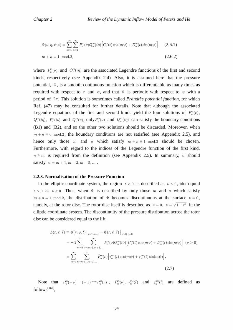
Chapter 2 Review of the Dynamic Inflow Model of Peters and He
34
Φ(, &, ψ, t) =∑
m=0
∞ ∑
n=1
∞Pmn ()Q
mn (i&)
[
Cmn (t) cos(mψ) +Dmn (t) sin(mψ)
]
, (2.6.1)
m + n 1 mod.2 , (2.6.2)
where Pmn () and Qmn (i&) are the associated Legendre functions of the first and second
kinds, respectively (see Appendix 2.4). Also, it is assumed here that the pressure
potential, Φ , is a smooth continuous function which is differentiable as many times as
required with respect to r and ψ , and that Φ is periodic with respect to ψ with a
period of 22. This solution is sometimes called Prandtl’s potential function, for which
Ref. (47) may be consulted for further details. Note that although the associated
Legendre equations of the first and second kinds yield the four solutions of Pmn (),
Qmn (i&), Pmn (i) and Qm
n (&), onlyPmn () and Qmn (i&) can satisfy the boundary conditions
(B1) and (B2), and so the other two solutions should be discarded. Moreover, when
m + n 0 mod.2 , the boundary conditions are not satisfied (see Appendix 2.5), and
hence only those m and n which satisfy m + n 1 mod.2 should be chosen.
Furthermore, with regard to the indices of the Legendre function of the first kind,
n m is required from the definition (see Appendix 2.5). In summary, n should
satisfy n = m + 1, m + 3, m + 5, .... .
2.2.3. Normalisation of the Pressure Function
In the elliptic coordinate system, the region z < 0 is described as > 0 , idem quod
z > 0 as < 0 . Thus, when Φ is described by only those m and n which satisfy
m + n 1 mod.2 , the distribution of Φ becomes discontinuous at the surface = 0 ,
namely, at the rotor disc. The rotor disc itself is described as & = 0, = 1 r2√
in the
elliptic coordinate system. The discontinuity of the pressure distribution across the rotor
disc can be considered equal to the lift.
L(r, ψ, t) Φ(r, ψ, t)
<0,&=0
Φ(r, ψ, t)>0,&=0
= 2∑
m=0
∞ ∑
n=m+1,m+3,...
∞Pmn ()Q
mn (i0)
[
Cmn (t) cos(mψ) +Dmn (t) sin(mψ)
]
( > 0)
∑
m=0
∞ ∑
n=m+1,m+3,...
∞Pmn ()
[
Amcn (t) cos(mψ) + Amsn (t) sin(mψ)
]
.
(2.7)
Note that Pmn ( ) = ( 1)m+nPmn () , Pmn (), A
mcn (t) and Amsn (t) are defined as
follows(165),
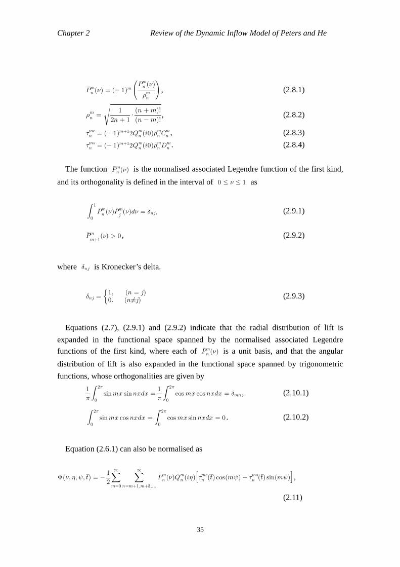
Chapter 2 Review of the Dynamic Inflow Model of Peters and He
35
Pmn () = ( 1)m mn
Pmn () )
, (2.8.1)
mn = 2n + 1
1 (n m)!(n +m)!
√
, (2.8.2)
Amcn = ( 1)m+12Qmn (i0)mnC
mn , (2.8.3)
Amsn = ( 1)m+12Qmn (i0)
mnD
mn . (2.8.4)
The function Pmn () is the normalised associated Legendre function of the first kind,
and its orthogonality is defined in the interval of 0 1 as
∫
0
1
Pmn ()Pmj()d = <nj, (2.9.1)
Pmm+1
() > 0 , (2.9.2)
where <nj is Kronecker’s delta.
<nj =1, (n = j)0. (n =j)
(2.9.3)
Equations (2.7), (2.9.1) and (2.9.2) indicate that the radial distribution of lift is
expanded in the functional space spanned by the normalised associated Legendre
functions of the first kind, where each of Pmn () is a unit basis, and that the angular
distribution of lift is also expanded in the functional space spanned by trigonometric
functions, whose orthogonalities are given by
2
1∫
0
22
sinmx sinnxdx =2
1∫
0
22
cosmx cos nxdx = <mn , (2.10.1)
∫
0
22
sinmx cos nxdx =
∫
0
22
cosmx sinnxdx = 0 . (2.10.2)
Equation (2.6.1) can also be normalised as
Φ(, &, ψ, t) = 2
1∑
m=0
∞ ∑
n=m+1,m+3,...
∞Pmn ()Q
mn (i&)
[
Amcn (t) cos(mψ) + Amsn (t) sin(mψ)
]
,
(2.11)
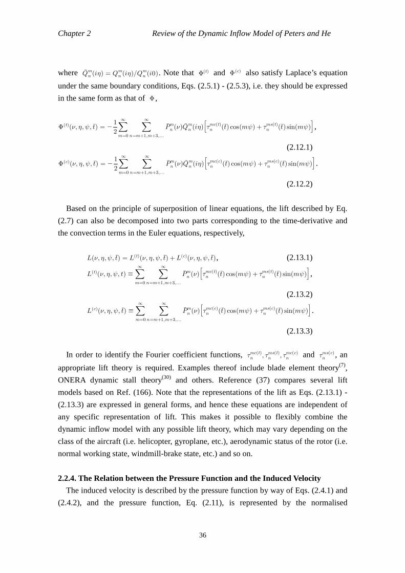
Chapter 2 Review of the Dynamic Inflow Model of Peters and He
36
where Qmn (i&) = Qmn (i&)/Q
mn (i0). Note that Φ(t) and Φ(c) also satisfy Laplace’s equation
under the same boundary conditions, Eqs. (2.5.1) - (2.5.3), i.e. they should be expressed
in the same form as that of Φ ,
Φ(t)(, &, ψ, t) = 2
1∑
m=0
∞ ∑
n=m+1,m+3,...
∞Pmn ()Q
mn (i&)
[
Amc(t)n (t) cos(mψ) + Ams(t)n (t) sin(mψ)]
,
(2.12.1)
Φ(c)(, &, ψ, t) = 2
1∑
m=0
∞ ∑
n=m+1,m+3,...
∞Pmn ()Q
mn (i&)
[
Amc(c)n (t) cos(mψ) + Ams(c)n (t) sin(mψ)]
.
(2.12.2)
Based on the principle of superposition of linear equations, the lift described by Eq.
(2.7) can also be decomposed into two parts corresponding to the time-derivative and
the convection terms in the Euler equations, respectively,
L(, &, ψ, t) = L(t)(, &, ψ, t) + L(c)(, &, ψ, t), (2.13.1)
L(t)(, &, ψ, t) ∑
m=0
∞ ∑
n=m+1,m+3,...
∞Pmn ()
[
Amc(t)n (t) cos(mψ) + Ams(t)n (t) sin(mψ)]
,
(2.13.2)
L(c)(, &, ψ, t) ∑
m=0
∞ ∑
n=m+1,m+3,...
∞Pmn ()
[
Amc(c)n (t) cos(mψ) + Ams(c)n (t) sin(mψ)]
.
(2.13.3)
In order to identify the Fourier coefficient functions, Amc(t)n , Ams(t)n , Amc(c)n and Ams(c)n , an
appropriate lift theory is required. Examples thereof include blade element theory(7),
ONERA dynamic stall theory(30) and others. Reference (37) compares several lift
models based on Ref. (166). Note that the representations of the lift as Eqs. (2.13.1) -
(2.13.3) are expressed in general forms, and hence these equations are independent of
any specific representation of lift. This makes it possible to flexibly combine the
dynamic inflow model with any possible lift theory, which may vary depending on the
class of the aircraft (i.e. helicopter, gyroplane, etc.), aerodynamic status of the rotor (i.e.
normal working state, windmill-brake state, etc.) and so on.
2.2.4. The Relation between the Pressure Function and the Induced Velocity
The induced velocity is described by the pressure function by way of Eqs. (2.4.1) and
(2.4.2), and the pressure function, Eq. (2.11), is represented by the normalised
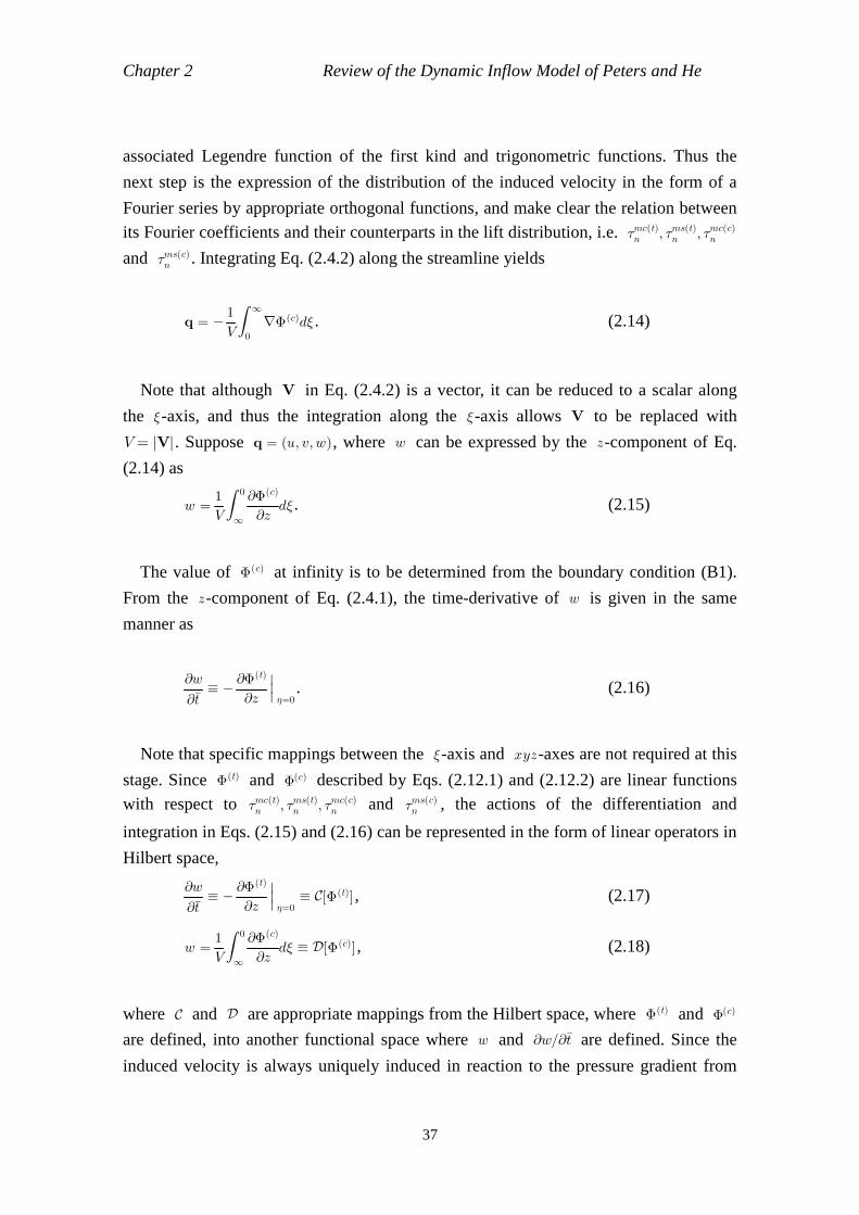
Chapter 2 Review of the Dynamic Inflow Model of Peters and He
37
associated Legendre function of the first kind and trigonometric functions. Thus the
next step is the expression of the distribution of the induced velocity in the form of a
Fourier series by appropriate orthogonal functions, and make clear the relation between
its Fourier coefficients and their counterparts in the lift distribution, i.e. Amc(t)n , Ams(t)n , Amc(c)n
and Ams(c)n . Integrating Eq. (2.4.2) along the streamline yields
q = V
1∫
0
∞∇Φ(c)d$ . (2.14)
Note that although V in Eq. (2.4.2) is a vector, it can be reduced to a scalar along
the $-axis, and thus the integration along the $-axis allows V to be replaced with
V = |V|. Suppose q = (u, v, w), where w can be expressed by the z-component of Eq.
(2.14) as
w =V
1∫
∞
0
∂z
∂Φ(c)d$ . (2.15)
The value of Φ(c) at infinity is to be determined from the boundary condition (B1).
From the z-component of Eq. (2.4.1), the time-derivative of w is given in the same
manner as
∂t
∂w ∂z
∂Φ(t)&=0
. (2.16)
Note that specific mappings between the $-axis and xyz-axes are not required at this
stage. Since Φ(t) and Φ(c) described by Eqs. (2.12.1) and (2.12.2) are linear functions
with respect to Amc(t)n , Ams(t)n , Amc(c)n and Ams(c)n , the actions of the differentiation and
integration in Eqs. (2.15) and (2.16) can be represented in the form of linear operators in
Hilbert space,
∂t
∂w ∂z
∂Φ(t)&=0
C[Φ(t)] , (2.17)
w =V
1∫
∞
0
∂z
∂Φ(c)d$ D[Φ(c)] , (2.18)
where C and D are appropriate mappings from the Hilbert space, where Φ(t) and Φ(c)
are defined, into another functional space where w and ∂w/∂t are defined. Since the
induced velocity is always uniquely induced in reaction to the pressure gradient from
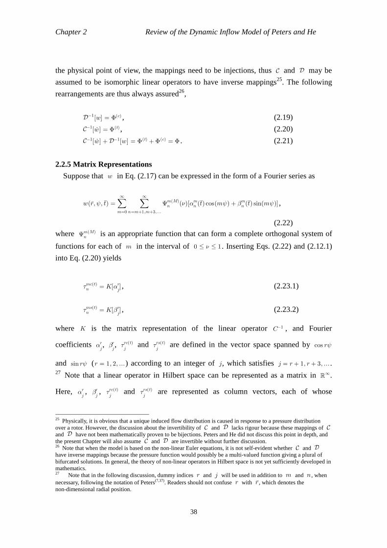
Chapter 2 Review of the Dynamic Inflow Model of Peters and He
38
the physical point of view, the mappings need to be injections, thus C and D may be
assumed to be isomorphic linear operators to have inverse mappings25. The following
rearrangements are thus always assured26,
D1[w] = Φ(c) , (2.19)
C1[w ] = Φ(t) , (2.20)
C1[w ] +D1[w] = Φ(t) +Φ(c) = Φ . (2.21)
2.2.5 Matrix Representations
Suppose that w in Eq. (2.17) can be expressed in the form of a Fourier series as
w(r, ψ, t) =∑
m=0
∞ ∑
n=m+1,m+3,...
∞Ψm(M)n ()[:mn (t) cos(mψ) + ;
mn (t) sin(mψ)] ,
(2.22)
where Ψm(M)n is an appropriate function that can form a complete orthogonal system of
functions for each of m in the interval of 0 1 . Inserting Eqs. (2.22) and (2.12.1)
into Eq. (2.20) yields
Amc(t)n = K[:rj] , (2.23.1)
Ams(t)n = K[;rj] , (2.23.2)
where K is the matrix representation of the linear operator C1 , and Fourier
coefficients :rj, ;r
j, Arc(t)
j and Ars(t)
j are defined in the vector space spanned by cos rψ
and sin rψ (r = 1, 2, ...) according to an integer of j, which satisfies j = r + 1, r + 3, ... . 27 Note that a linear operator in Hilbert space can be represented as a matrix in R
∞.
Here, :rj, ;r
j, Arc(t)
j and Ars(t)
j are represented as column vectors, each of whose
25 Physically, it is obvious that a unique induced flow distribution is caused in response to a pressure distribution over a rotor. However, the discussion about the invertibility of C and D lacks rigour because these mappings of C and D have not been mathematically proven to be bijections. Peters and He did not discuss this point in depth, and the present Chapter will also assume C and D are invertible without further discussion. 26 Note that when the model is based on the non-linear Euler equations, it is not self-evident whether C and D have inverse mappings because the pressure function would possibly be a multi-valued function giving a plural of bifurcated solutions. In general, the theory of non-linear operators in Hilbert space is not yet sufficiently developed in mathematics. 27 Note that in the following discussion, dummy indices r and j will be used in addition to m and n , when necessary, following the notation of Peters(7,37). Readers should not confuse r with r, which denotes the non-dimensional radial position.
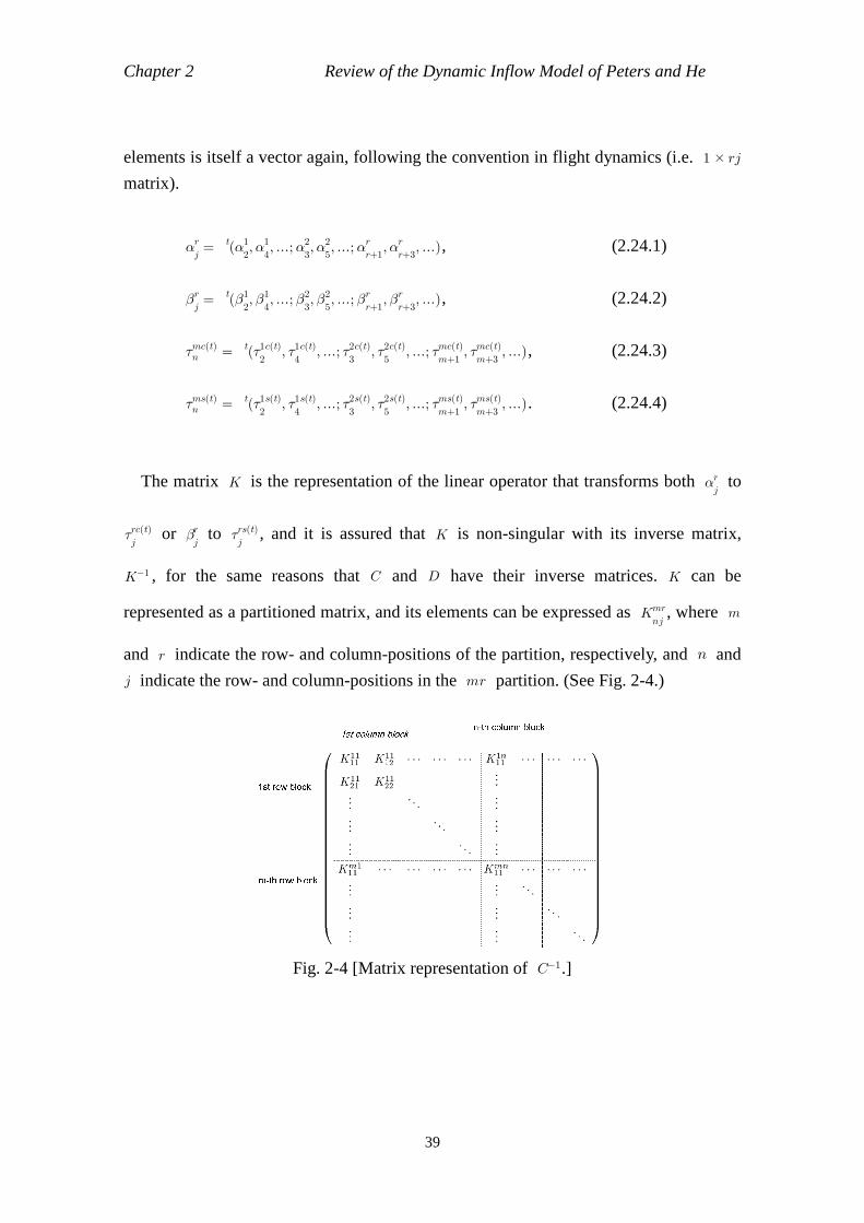
Chapter 2 Review of the Dynamic Inflow Model of Peters and He
39
elements is itself a vector again, following the convention in flight dynamics (i.e. 1 rj matrix).
:rj= t(:1
2, :1
4, ...;:2
3, :2
5, ...;:r
r+1, :r
r+3, ...), (2.24.1)
;rj= t(;1
2, ;1
4, ...; ;2
3, ;2
5, ...; ;r
r+1, ;r
r+3, ...), (2.24.2)
Amc(t)n = t(A1c(t)2
, A1c(t)4
, ...; A2c(t)3
, A2c(t)5
, ...; Amc(t)m+1
, Amc(t)m+3
, ...), (2.24.3)
Ams(t)n = t(A1s(t)2
, A1s(t)4
, ...; A2s(t)3
, A2s(t)5
, ...; Ams(t)m+1
, Ams(t)m+3
, ...). (2.24.4)
The matrix K is the representation of the linear operator that transforms both :rj to
Arc(t)j
or ;rj to Ars(t)
j, and it is assured that K is non-singular with its inverse matrix,
K1 , for the same reasons that C and D have their inverse matrices. K can be
represented as a partitioned matrix, and its elements can be expressed as Kmr
nj, where m
and r indicate the row- and column-positions of the partition, respectively, and n and
j indicate the row- and column-positions in the mr partition. (See Fig. 2-4.)
Fig. 2-4 [Matrix representation of C1.]
Chapter 2 Review of the Dynamic Inflow Model of Peters and He
40
For its inverse matrix to exist, the matrix K needs to be regular28. Suppose also that
w in Eq. (2.18) can be expressed in the same form as ω in Eq. (2.22),
w(r, ψ, t) =∑
m=0
∞ ∑
n=m+1,m+3,...
∞Ψm(L)n ()[=mn (t) cos(mψ) +
mn (t) sin(mψ)] ,
(2.25)
where Ψm(L)n is also an appropriate function which can form a complete orthogonal
system of functions for each m in the interval of 0 1 . Note that Ψm(L)n in Eq.
(2.25) may be different from Ψm(M)n in Eq. (2.22), because Eqs. (2.19) and (2.20) are
independent. Inserting Eqs. (2.25) and (2.12.2) into Eq. (2.19) yields the following
equations,
Amc(c)n = Y1[=r
j], (2.26)
Ams(c)n = Y1[r
j] , (2.27)
where Y is the matrix representation of the linear operator D. Here again, =r
j, r
j,
Arc(c)j
and Ars(c)j
are defined in the functional space spanned by cos rψ and sin rψ
(r = 1, 2, ...) according to an integer j, which satisfies j = r + 1, r + 3, .... .
=rj= t(=1
2, =14, ...; =2
3, =25, ...; =r
r+1, =rr+3, ...), (2.28.1)
r
j= t(1
2, 1
4, ...;2
3, 2
5, ...;r
r+1, r
r+3, ...), (2.28.2)
Amc(c)n = t(A1c(c)2
, A1c(c)4
, ...; A2c(c)3
, A2c(c)5
, ...; Amc(c)m+1
, Amc(c)m+3
, ...), (2.28.3)
Ams(c)n = t(A1s(c)2
, A1s(c)4
, ...; A2s(c)3
, A2s(c)5
, ...; Ams(c)m+1
, Ams(c)m+3
, ...). (2.28.4)
The matrix Y has its inverse matrix Y1 for the same reason why the inverse of K exists. The matrix Y may be considered as a partitioned matrix, transforming both =r
j
to Amc(c)n and rj to Ams(c)n . The elements of the matrix Y can be expressed as Yrm
nj,
where m and r indicate the row- and column-block positions in a partitioned matrix,
28 The matrix K may be intuitively considered as a square matrix, although both m and r are ideally in the range 0 to ∞.
Chapter 2 Review of the Dynamic Inflow Model of Peters and He
41
respectively, and n and j indicate the row- and column-positions in the mr partition,
respectively, as illustrated in Fig. 2-4. Equations (2.4.3), (2.23.1), (2.23.2), (2.26) and
(2.27) yield the following matrix equations,
[
Kmr
nj
]
: rj
)
+
[
Ymrcnj
]1
=rj
)
=
Amc(t)n
)
+
Amc(c)n
)
=
Amcn
)
,
(2.29.1)
[
Kmr
nj
]
; rj
)
+
[
Ymrsnj
]1
r
j
)
=
Ams(t)n
)
+
Ams(c)n
)
=
Amsn
)
.
(2.29.2)
Note that while m 0 in Eq. (2.29.1), m 1 in Eq. (2.29.2). Note also that n
should satisfy n > m, n +m 1 mod.2 (i.e. n = m + 1, m + 3, m + 5, ... ) in both
equations. When these equations are numerically computed, the integers m, r, n and j
need to be truncated at an appropriate finite number so that Krm
nj and Yrm
nj should be
finite-dimensional square matrices, for which maxr = maxm is necessary.
2.2.6 The Unified Representation of the Induced Flow Fields
Equations (2.29.1) and (2.29.2) are expressed in terms of Fourier coefficients :rj, ;r
j, =rj
and r
j to represent the same induced velocity distribution, but, in fact, only two of
these sets of coefficients are sufficient to represent any flow field. Thus, appropriate transformations represented by matrices Akr
ij and Bkr
ij are introduced to unify the
representations such that
[
Kmk
ni
][
Akrij
]
a rj
)
+
[
Ymkcni
]1[
Bkrij
]
arj
)
=
Amc(t)n
)
+
Amc(c)n
)
=
Amcn
)
,
(2.30.1) [
Kmk
ni
][
Akrij
]
b rj
)
+
[
Ymksni
]1[
Bkrij
]
brj
)
=
Ams(t)n
)
+
Ams(c)n
)
=
Amsn
)
,
(2.30.2)
where
[
Akrij
]
a rj
)
=
: ki
)
, (2.31.1)
Chapter 2 Review of the Dynamic Inflow Model of Peters and He
42
[
Akrij
]
b rj
)
=
; ki
)
, (2.31.2)
[
Bkrij
arj
)
=
=ki
)
, (2.31.3)
[
Bkrij
]
brj
)
=
k
i
)
, (2.31.4)
w(r, ψ, t) =∑
r=0
∞ ∑
j=r+1,r+3,...
∞Ψrj()[ar
j(t) cos(rψ) + br
j(t) sin(rψ)] . (2.32)
Equations (2.30.1) and (2.30.2) can be rewritten as
[
Mmr
nj
]
a rj
)
+
[
Lmrcnj
]1
arj
)
=
Amc(t)n
)
+
Amc(c)n
)
=
Amcn
)
, (2.33.1)
[
Mmr
nj
]
b rj
)
+
[
Lmrcnj
]1
brj
)
=
Ams(t)n
)
+
Ams(c)n
)
=
Amsn
)
, (2.33.2)
where
[
Mmr
nj
=
[
Kmk
ni
][
Akrij
]
, (2.34.1)
[
Lmrcnj
]1
=
[
Ymkcni
]1[
Bkrij
, (2.34.2)
[
Lmrsnj
]1
=
[
Ymksni
]1[
Bkrij
]
. (2.34.3)
Equations (2.33.1) and (2.33.2) can be decomposed again into a time-derivative and
convection parts as, respectively,
[
Mmr
nj
]
a rj
)
=
Amc(t)n
)
, (2.35.1)
[
Mmr
nj
]
b rj
)
=
Ams(t)n
)
, (2.35.2)
[
Lmrcnj
]1
arj
)
=
Amc(c)n
)
, (2.35.3)
[
Lmrsnj
]1
brj
)
=
Ams(c)n
)
. (2.35.4)
Chapter 2 Review of the Dynamic Inflow Model of Peters and He
43
These matrix equations of Eqs. (2.33.1) and (2.33.2) are well-known as the typical
forms of the dynamic inflow model, though the basic structures of these equations are
essentially those of the Euler equations, Eq. (2.3). Whereas Ψrj may be any appropriate
function in so far as it can form a complete orthogonal system of functions for each m
in the interval of [0, 1] , Peters recommended purely from a practical point of view in Refs. (37) and (92) that (1/)Pr
j() may be the best choice on account of the rapid
convergence of these functions around r = 1 (i.e. around the blade tip), and also of the
practical feasibility that arises from the fact that computations with these functions may
be carried out analytically in a closed form(37)(92),
Ψrj=
1Prj(). (2.36)
The remaining problem is how to define Ψm(L)n and Ψm(M)n , and Peters also
recommended the following representations again from a practical point of view.
Ψr(M)j
=
1Prj(), (2.37.1)
Ψr(L)j
= Prj(). (2.37.2)
As well as the fact that (1/)Prj() forms a complete orthogonal system of functions,
it can also be expressed in terms of only the radial position of the rotor disc, r= 1 2√
,
and this property hugely simplifies the practical treatment of the equations in relation to
the blade element theory (see also Appendix 2.7),
1Pmn () = (2n + 1)Hm
n
√ ∑
q=m,m+2,m+4,...
n1
(q m)!!(q +m)!!(n q 1)!!( 1) 2
qm(n + q)!!
rq,
(2.38)
where
Hmn = (n +m)!!(n m)!!
(n +m 1)!!(n m 1)!!. (2.39)
For the case when n = m + 1 , Eq. (2.38) can be further simplified as follows(92),
1Pmm+1
() =(2m)!!
(2m + 3)!!√
rm. (2.40)
Chapter 2 Review of the Dynamic Inflow Model of Peters and He
44
In the later discussion, Ψrj is to be integrated over the rotor disc, and the fact that
(1/)Pmn () is a function of r alone makes the integration much simpler. Equation
(2.40) is of particular use for that case29. Equations (2.33.1), (2.34.1) and (2.35.1) allow
of the assumption that, without the loss of generality,
Akrij
= <ij, (2.41)
:rj= ar
j. (2.42)
Thus, the matrix Akrij
becomes the unit matrix. In this case, the matrix Bkrij
should be
determined through substituting Eqs. (2.26), (2.31.3), (2.31.4), (2.34.2), (2.34.3),
(2.35.3), (2.35.4), (2.36) and (2.27) into Eq. (2.18) and equating coefficients. Regarding
the cosine terms, substituting Eqs (2.23.2), (2.25), (2.36) and (2.37.2) into Eq. (2.34.2)
yields
∑
r=0
∞ ∑
j=r+1,r+3,...
∞
1Prj()[ar
j(t) cos(rψ) + br
j(t) sin(rψ)]
=∑
k=0
∞ ∑
i=k+1,k+3,...
∞Pki()[=k
i(t) cos(kψ) +k
i(t) sin(kψ)] . (2.43)
On account of the orthogonality of normalised associated Legendre functions of the
first kind over [0, 1] , Eq.(2.9.1), and of the trigonometric functions over [0, 22] (Eq.
(2.10.1) and (2.10.2)), =ki and k
i can be determined as
=ki=2
1∫
0
22∫
0
1∑
r=0
∞ ∑
j=r+1,r+3,...
∞
1Prj()[ar
j(t) cos(rψ) + br
j(t) sin(rψ)]
Pki() cos(kψ)ddψ
=∫
0
1
1Prj()Pk
i()d
arj, (2.44)
29 Also, as is often the case with application to flight control systems, only a crude approximation is required where n is simply considered to be m + 1 .
Chapter 2 Review of the Dynamic Inflow Model of Peters and He
45
k
i=2
1∫
0
22∫
0
1∑
r=0
∞ ∑
j=r+1,r+3,...
∞
1Prj()[ar
j(t) cos(rψ) + br
j(t) sin(rψ)]
Pki() sin(kψ)ddψ
=∫
0
1
1Prj()Pk
i()d
brj. (2.45)
Thus, from Eqs. (2.31.1) and (2.31.4),
Bkrij=
∫
0
1
1Prj()Pk
i()d . (2.46.1)
Note that matrix [Bkrij] does not have to have non-zero values for its entries; in fact, a
diagonal partition matrix suffices for the transformation required in Eqs. (2.31.3) and
(2.31.4).
Bkij=
∫
0
1
1Pkj()Pk
i()d . (2.46.2)
This integration can be analytically expressible and the formula is found in Ref.
(167).
∫
0
1
1Pkj()Pk
i()d = ( 1)i+j2r2 (2i + 1)(2j+ 1)
Hk
i
Hk
j
√√√√√
∑
q=r,r+2,...
j1
(i q)(i + q + 1)(2q + 1)
Hkq .
(2.47)
The inverse matrix of Bkij was found by He (Ref. (7), page 30),
[
Bkij
]1=
Hk
jHk
i
√( 1) 2
i+j2r
(i + j)(i + j+ 2)[(i j)2 1]
2 (2i + 1)(2j+ 1)√
, (2.48)
where this expression will be highly convenient for the later discussion of Lmrc
nj and
Lmrsnj
.
Chapter 2 Review of the Dynamic Inflow Model of Peters and He
46
2.2.7 The Apparent Mass Matrix, M
In order to combine Eq. (2.36) with Eq. (2.17), the z-derivative in Eq. (2.17) should
be transformed into ellipsoidal coordinates30 (see Appendix 2.3). In general,
∂z
∂=
2 + &21
&(1 2)∂
∂+ (1 + &2)
∂&
∂
. (2.49)
In particular, on the rotor disc & = 0 , and hence Equation (2.49) can be simplified to
∂z
∂rotor disc
=
1 ∂&
∂. (2.50)
Equations (2.17) and (2.50) yield
v i = w ∂z
∂Φ(t)&=0
=
1 ∂&
∂Φ(t)&=0
. (2.51)
On the other hand, Eqs. (2.12.1) and (2.22) give
1 ∂&
∂Φ(t)&=0
= 2
1∑
m=0
∞ ∑
n=m+1,m+3,...
∞
1Pmn () ∂&
∂Qmn (i&)[
Amc(t)n (t) cos(mψ) + Ams(t)n (t) sin(mψ)]&=0
,
(2.52)
w =∑
r=0
∞ ∑
j=r+1,r+3,...
∞
1Prj()[a r
j(t) cos(rψ) + b r
j(t) sin(rψ)] . (2.53)
Substituting Eqs. (2.50), (2.52) and (2.53) into Eq. (2.17) yields
∑
r=0
∞ ∑
j=r+1,r+3,...
∞Prj()[a r
j(t) cos(rψ) + b r
j(t) sin(rψ)]
= 2
1∑
m=0
∞ ∑
n=m+1,m+3,...
∞Pmn () ∂&
∂Qmn (i&)[
Amc(t)n (t) cos(mψ) + Ams(t)n (t) sin(mψ)]&=0
.
(2.54) Multiplying Eq. (2.54) by Pr
j() and cos(rψ), and integrating by over [0, 1] and
by ψ over [0, 22] , the orthogonality of the normalised associated Legendre function of
30 References (1) and (35) contain the same typographical error in the representation of Eq. (2.49).
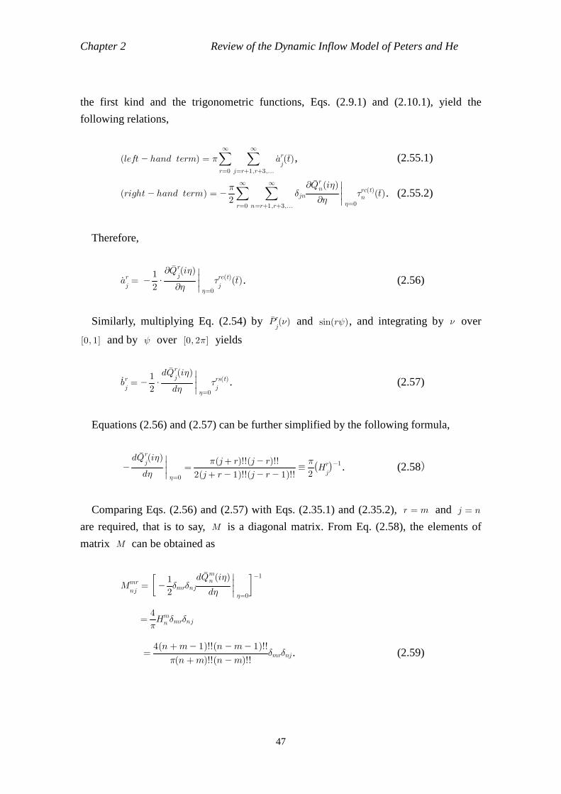
Chapter 2 Review of the Dynamic Inflow Model of Peters and He
47
the first kind and the trigonometric functions, Eqs. (2.9.1) and (2.10.1), yield the
following relations,
(left hand term) = 2∑
r=0
∞ ∑
j=r+1,r+3,...
∞a rj(t), (2.55.1)
(right hand term) = 2
2∑
r=0
∞ ∑
n=r+1,r+3,...
∞<jn
∂&
∂Q rn(i&)&=0
Arc(t)n (t). (2.55.2)
Therefore,
a rj=
2
1 ∂&
∂Q rj(i&)
&=0
Arc(t)j
(t). (2.56)
Similarly, multiplying Eq. (2.54) by Pr
j() and sin(rψ), and integrating by over
[0, 1] and by ψ over [0, 22] yields
b rj=
2
1 d&
dQ rj(i&)
&=0
Ars(t)j
. (2.57)
Equations (2.56) and (2.57) can be further simplified by the following formula,
d&
dQ rj(i&)
&=0
=2(j+ r 1)!!(j r 1)!!
2(j+ r)!!(j r)!! 2
2Hrj
1 . (2.58)
Comparing Eqs. (2.56) and (2.57) with Eqs. (2.35.1) and (2.35.2), r = m and j = n
are required, that is to say, M is a diagonal matrix. From Eq. (2.58), the elements of
matrix M can be obtained as
Mmr
nj=
2
1<mr<nj
d&
dQmn (i&)&=0
1
=2
4Hmn <mr<nj
=2(n +m)!!(n m)!!
4(n +m 1)!!(n m 1)!!<mr<nj. (2.59)
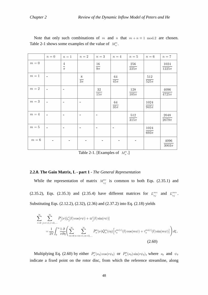
Chapter 2 Review of the Dynamic Inflow Model of Peters and He
48
Note that only such combinations of m and n that m + n 1 mod.2 are chosen.
Table 2-1 shows some examples of the value of Mmn .
n = 0 n = 1 n = 2 n = 3 n = 4 n = 5 n = 6 n = 7
m = 0 2
4
92
16
2252
256
12252
1024
m = 1 - 32
8
452
64
5252
512
m = 2 - - 152
32
1052
128
47252
4096
m = 3 - - - 352
64
9452
1024
m = 4 - - - - 3152
512
20792
2048
m = 5 - - - - - 6932
1024
m = 6 - - - - - - 30032
4096
Table 2-1. [Examples of Mmn .]
2.2.8. The Gain Matrix, L - part 1 - The General Representation
While the representation of matrix Mmr
nj is common to both Eqs. (2.35.1) and
(2.35.2), Eqs. (2.35.3) and (2.35.4) have different matrices for Lmrcnj
and Lmrsnj
.
Substituting Eqs. (2.12.2), (2.32), (2.36) and (2.37.2) into Eq. (2.18) yields
∑
r=0
∞ ∑
j=r+1,r+3,...
∞Prj()[=r
j(t) cos(rψ) +r
j(t) sin(rψ)]
=2V
1∫
0
∞
1
∂&
∂
∑
m=0
∞ ∑
n=m+1,m+3,...
∞Pmn ()Q
mn (i&)
[
Amc(c)n (t) cos(mψ) + Ams(c)n (t) sin(mψ)
)
d$ .
(2.60)
Multiplying Eq. (2.60) by either Pmn (0) cos(rψ0) or Pmn (0) sin(rψ0), where 0 and ψ0
indicate a fixed point on the rotor disc, from which the reference streamline, along
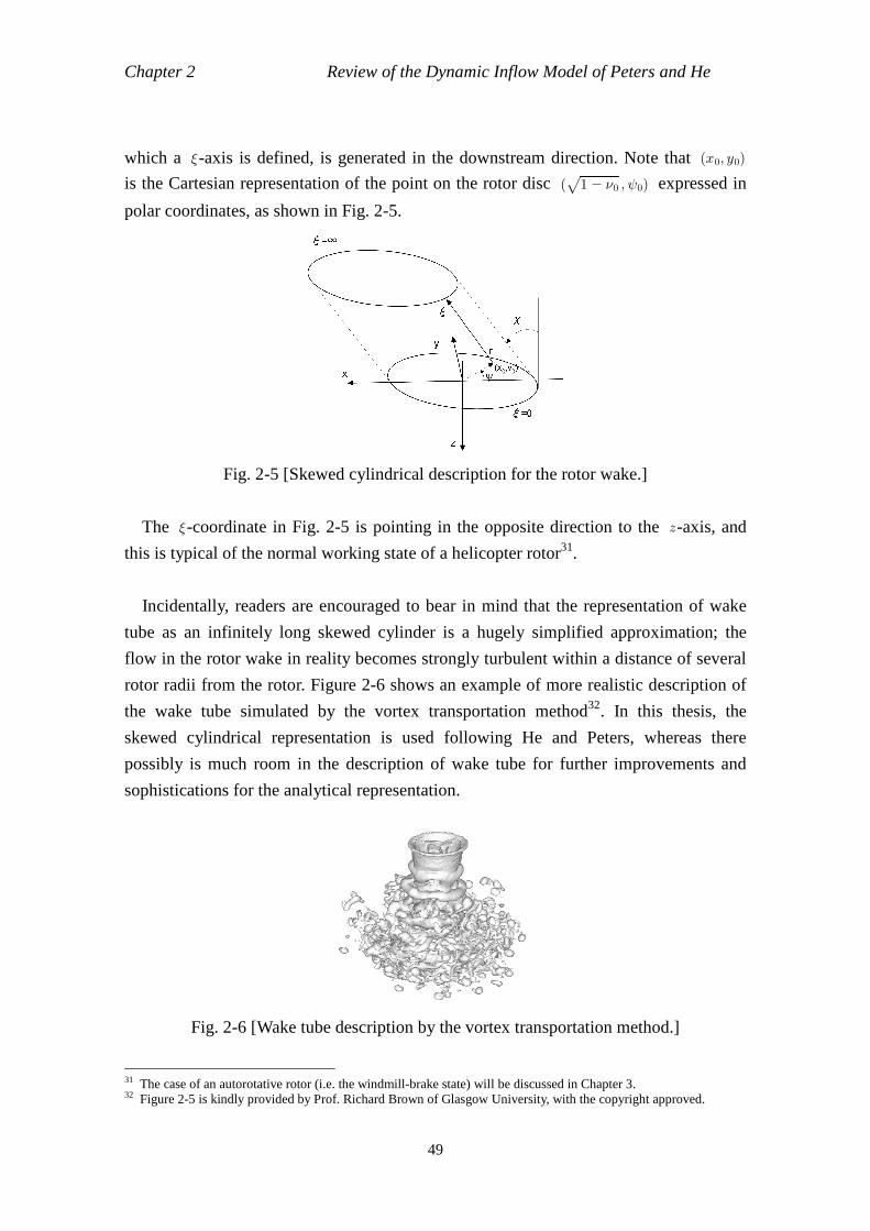
Chapter 2 Review of the Dynamic Inflow Model of Peters and He
49
which a $-axis is defined, is generated in the downstream direction. Note that (x0, y0)
is the Cartesian representation of the point on the rotor disc ( 1 0√
, ψ0) expressed in
polar coordinates, as shown in Fig. 2-5.
Fig. 2-5 [Skewed cylindrical description for the rotor wake.]
The $-coordinate in Fig. 2-5 is pointing in the opposite direction to the z-axis, and
this is typical of the normal working state of a helicopter rotor31.
Incidentally, readers are encouraged to bear in mind that the representation of wake
tube as an infinitely long skewed cylinder is a hugely simplified approximation; the
flow in the rotor wake in reality becomes strongly turbulent within a distance of several
rotor radii from the rotor. Figure 2-6 shows an example of more realistic description of
the wake tube simulated by the vortex transportation method32. In this thesis, the
skewed cylindrical representation is used following He and Peters, whereas there
possibly is much room in the description of wake tube for further improvements and
sophistications for the analytical representation.
Fig. 2-6 [Wake tube description by the vortex transportation method.]
31 The case of an autorotative rotor (i.e. the windmill-brake state) will be discussed in Chapter 3. 32 Figure 2-5 is kindly provided by Prof. Richard Brown of Glasgow University, with the copyright approved.
Chapter 2 Review of the Dynamic Inflow Model of Peters and He
50
Integrating Eq. (2.60) by 0 over [0, 1] and by ψ over [0, 22], the orthogonality of
the normalised associated Legendre functions of the first kind and trigonometric
functions give the following relations,
2∑
r=0
∞ ∑
j=r+1,r+3,...
∞=rj(t)
=
[∫
0
22∫
0
1
2V
1∫
0
∞
∂&
∂
∑
m=0
∞ ∑
n=m+1,m+3,...
∞Pmn ()Q
mn (i&) cos(mψ)
)
d$ Prj(0) cos(rψ)d0dΨ
]
Amc(c)n (t),
(2.61)
2∑
r=0
∞ ∑
j=r+1,r+3,...
∞rj(t)
=
[∫
0
22∫
0
1
2V
1∫
0
∞
∂&
∂
∑
m=0
∞ ∑
n=m+1,m+3,...
∞Pmn ()Q
mn (i&) sin(mψ)
)
d$ Pmn (0) sin(rψ)d0dΨ]
Ams(c)n (t).
(2.62)
From Eqs. (2.35.3), (2.35.4), (2.61) and (2.62), the elements of matrices Lrmcjn and
Lrmsjn can be expressed as follows,
Lmrcnj
=22V
1∫
0
22∫
0
1∫
0
∞
∂&
∂
Pmn ()Qmn (i&) cos(mψ)
)
d$ Prj(0) cos(rψ)d0dψ ,
(2.63)
Lmrsnj
=22V
1∫
0
22∫
0
1∫
0
∞
∂&
∂
Pmn ()Qmn (i&) sin(mψ)
)
d$ Prj(0) sin(rψ)d0dψ .
(2.64)
Regarding the definition of the gain matrix, Peters presented a different form(37), in
which the mass-flow parameter, V , is excluded. This form is distinguished from Eqs.
(2.63) and (2.64) by hat symbol, (^), following Peters’ notation.
L rmcjn
=22
1∫
0
22∫
0
1∫
0
∞
∂&
∂
Pmn ()Qmn (i&) cos(mψ)
)
d$ Prj(0) cos(rψ)d0dψ , (2.65.1)
L rmsjn
=22
1∫
0
22∫
0
1∫
0
∞
∂&
∂
Pmn ()Qmn (i&) sin(mψ)
)
d$ Prj(0) sin(rψ)d0dψ , (2.65.2)
L 0mcjn
=42
1∫
0
22∫
0
1∫
0
∞
∂&
∂
Pmn ()Qmn (i&) cos(mψ)
)
d$ P0j(0)d0dψ . (2.65.3)
Chapter 2 Review of the Dynamic Inflow Model of Peters and He
51
Note that L0mcjn has the coefficient of 1/4 while Lrmcjn and Lrmsjn have 1/2 . (See
Appendix 2.8 thereabout.) Note also that when r = 0 , the associated Legendre function
of the first kind reduces to the Legendre function of the first kind (see Appendix 2.5).
The integrations of Eqs. (2.65.1) - (2.65.3) will be discussed in the next Subsection33.
2.2.9 The Gain Matrix, L - part 2 - Skewed Cylindrical Representation for the Wake
Tube
Using Eqs. (2.12.2) and (2.50), Eqs (2.65.1) - (2.65.3) can be rearranged as
L rmcjn
=22
1∫
0
22∫
0
1∫
0
∞
∂z
∂Φmc(c)nd$ Pr
j(0) cos(rψ)d0dψ , (2.66.1)
L rmsjn
=22
1∫
0
22∫
0
1∫
0
∞
∂z
∂Φms(c)nd$ Pr
j(0) sin(rψ)d0dψ , (2.66.2)
L 0mcjn
=42
1∫
0
22∫
0
1∫
0
∞
∂z
∂Φmc(c)nd$ P0
j(0)d0dψ . (2.66.3)
In spite of the apparent complicated forms of these expressions, it is shown by He
that these integrations are analytically expressible in closed forms in Ref. (7), and his
method will be revisited in this Subsection. First of all, it should be confirmed that He’s
method is based on the following assumptions34:
(C1) the wake tube should be described as a skewed cylinder with the wake skew
angle of 1 to the rotor disc, as is shown in Fig. 2-535;
(C2) the wake skew angle, 1, should be small36.
Suppose the rotor wake is expressed in the shape of skewed cylinder following He,
33 With regard to the coefficient of Lmr
nj , there are variations in the literature: for example, Refs. (92) and (37)
introduce different Lmr
nj where the former is double as of the latter. See Appendix 2.9 about the variation in the
definition. 34 These assumptions are not mentioned at all in Refs. (1), (37), (92) and (112), and are mentioned only in an appendix of Ref. (7). Most readers who have not read Ref. (7) may thus perhaps struggle to execute the integrations of Eq. (2.65) and how to determine the elements of the gain matrix. 35 As mentioned in the previous Subsection, assumption (C1) is controversial. However, it is highly likely impossible to analytically perform the complicated integrations in Eqs. (2.66.1) - (2.66.3) without the simplification. Even in more advanced augmented dynamic inflow models (e.g. Ref. (129)), in which more convoluted wake distortion is considered, only ad hoc coefficients modifying the Peter and He model are used to represent the wake distortion. It is likely that this is due to the hopeless complexity of those integrations when incorporating the wake distortion into the analytical calculation at this stage. 36 In high speed forward flight, the wake skew angle cannot be considered small. Thus for this flight situation, the justification for assumption (C2) also weakens. However, the validity of this assumption is not discussed in any of the previous studies, although the Peters and He model is widely used for flight dynamics applications even in full forward flight condition. The assumption shall be further discussed in Chapter 4.
Chapter 2 Review of the Dynamic Inflow Model of Peters and He
52
these integrations can be considered as volume integrations throughout the skewed
cylindrical domain shown in Fig. 2-5. The one-dimensional $-coordinate is defined
inside the skewed cylinder along a streamline. A point inside the skewed cylinder,
(x, y, z), can be described by $ and (x0, y0), which is a specific point on the rotor disc
from which the reference streamline develops in the downstream direction (see also
Appendix 2.2).
x = $ sin1+ x0 , (2.67.1)
y = y0 , (2.67.2)
z = $ cos1, (2.67.3)
where
x0 = rcos ψ , (2.68.1)
y0 = rsinψ . (2.68.2)
Equations (2.67.1), (2.67.2) and (2.67.3) in turn give the following relations,
d$ = cos1
1dz, (2.69.1)
∂$
∂=∂$
∂x ∂x
∂+∂$
∂y ∂y
∂+∂$
∂z ∂z
∂= sin1
∂x
∂ cos1∂z
∂. (2.69.2)
Note that cos 1=0 is necessary when deriving Eq. (2.69.1) from Eq. (2.67.3), thus
edgewise flight (1 = 2/2) should be excluded from the model hereinafter37.
From Eq. (2.69.2),
∂z
∂=
cos 1
1 ∂$
∂+ tan1
∂x
∂. (2.70)
Using Eq. (2.70), Eq. (2.66.1) can be rearranged as
L rmcjn
=22
1∫
0
22∫
0
1∫
0
∞
∂z
∂Φmc(c)nd$ Pr
j(0) cos(rψ)d0dψ
= 22 cos 1
1∫
0
22∫
0
1∫
0
∞
∂$
∂Φmc(c)nd$ Pr
j(0) cos(rψ)d0dψ
+22
tan1∫
0
22∫
0
1∫
0
∞
∂x
∂Φmc(c)nd$ Pr
j(0) cos(rψ)d0dψ . (2.71)
37 However, the resultant model based on these equations will later be extended up to 1 = 2/2 owing to the small wake skew angle assumption. The extension of the model apparently contradicts the necessary condition for rearranging Eq. (2.67.3) to Eq. (2.69.1). This author will discuss this point in depth in Chapter 4.

Chapter 2 Review of the Dynamic Inflow Model of Peters and He
53
The first term on the right-hand side of Eq. (2.71) can be straightforwardly integrated
as
(first term) = 22 cos 1
1∫
0
22∫
0
1
Φmc(c)n
∞
0
Prj(0) cos(rψ)d0dψ
=22 cos 1
1∫
0
22∫
0
1
Φmc(c)n
$=0
Prj(0) cos(rψ)d0dψ
=22 cos 1
1∫
0
22∫
0
1
Pmn (0) cos(mψ)
)
Prj(0) cos(rψ)d0dψ
=2 cos 1
1<mr<nj. (2.72)
Note that Φmc(c)n
$=∞
= 0 by applying the boundary condition (B1). Using Eq.
(2.69.1), the second term on the right-hand side of Eq. (2.71) can be rearranged as
(second term) = 22 cos 1
tan1∫
0
22∫
0
1∫
0
∞
∂x
∂Φmc(c)ndz Pr
j(0) cos(rψ)d0dψ .
(2.73)
The same discussion can be applied to Eq. (2.66.2),
L rmsjn
=22
1∫
0
22∫
0
1∫
0
∞
∂z
∂Φms(c)nd$ Pr
j(0) sin(rψ)d0dψ
= 22 cos 1
1∫
0
22∫
0
1∫
0
∞
∂$
∂Φms(c)nd$ Pr
j(0) sin(rψ)d0dψ
+22
tan1∫
0
22∫
0
1∫
0
∞
∂x
∂Φms(c)nd$ Pr
j(0) sin(rψ)d0dψ , (2.74)
where
(first term) = 22 cos 1
1∫
0
22∫
0
1
Φms(c)n
∞
0
Prj(0) sin(rψ)d0dψ
=2 cos 1
1<mr<nj, (2.75)
(second term) = 22 cos 1
tan1∫
0
22∫
0
1∫
0
∞
∂x
∂Φms(c)ndz Pr
j(0) sin(rψ)d0dψ .
(2.76)
Chapter 2 Review of the Dynamic Inflow Model of Peters and He
54
Equation (2.66.3) is a special case of Eq. (2.66.1) in which r = 0 . In summary, Eqs.
(2.66.1) - (2.66.3) can be rearranged as follows,
L rmcjn
=2 cos 1
1<mr<nj
22 cos 1
tan1∫
0
22∫
0
1∫
0
∞
∂x
∂Φmc(c)ndz
Prj(0) cos(rψ)d0dψ , (2.77.1)
L rmsjn
=2 cos 1
1<mr<nj
22 cos 1
tan1∫
0
22∫
0
1∫
0
∞
∂x
∂Φms(c)ndz
Prj(0) sin(rψ)d0dψ ,(2.77.2)
L 0mcjn
=4 cos 1
1<mr<nj
42 cos 1
tan1∫
0
22∫
0
1∫
0
∞
∂x
∂Φmc(c)ndz
Prj(0)d0dψ . (2.77.3)
2.2.10 The Gain Matrix, L - part 3 - The Pressure Function From Eq. (2.12.2), Φmc(c)n and Φms(c)n can be expressed as follows,
Φmc(c)n = Pmn ()Qmn (i&) cos(mψ) = 2
eimψ + eimψPmn ()Q
mn (i&), (2.78.1)
Φms(c)n = Pmn ()Qmn (i&) sin(mψ) = 2i
eimψ eimψPmn ()Q
mn (i&). (2.78.2)
Note that the partial derivative with respect to x can be expressed in polar
coordinates as
∂x
∂=2
1
eiψ
∂r
∂+ir
1 ∂ψ
∂
eiψ
∂r
∂+ir
1 ∂ψ
∂
. (2.79)
Equations (2.78.1) and (2.79) yield the expression of the successive differentiation of
Φmc(c)n with respect to x .
∂xk
∂kΦmc(c)n=2k+11
eiψ
∂r
∂+ir
1 ∂ψ
∂
eiψ
∂r
∂+ir
1 ∂ψ
∂k
(eimψ + eimψ)Pmn ()Qmn (i&),
(2.80.1)
∂xk
∂kΦms(c)n=2k+1i
1
eiψ
∂r
∂+ir
1 ∂ψ
∂
eiψ
∂r
∂+ir
1 ∂ψ
∂k(eimψ eimψ)Pmn ()Q
mn (i&).
(2.80.2)
Chapter 2 Review of the Dynamic Inflow Model of Peters and He
55
For example, the first and second derivatives of Φmc(c)n and Φms(c)n are expressed as
follows38,
∂x
∂Φmc(c)n=221
(ei(m+1)ψ + ei(m+1)ψ)
∂r
∂+r
m
+ (ei(m1)ψ + ei(m1)ψ)
∂r
∂ r
m
Pmn ()Qmn (i&), (2.81.1)
∂x2
∂2Φmc(c)n=221
(ei(m+2)ψ + ei(m+2)ψ)
∂r
∂+
r
m + 1
∂r
∂+r
m
+ (ei(m2)ψ + ei(m2)ψ)
∂r
∂ r
m 1
∂r
∂ r
m
+ 2(eimψ + eimψ)
∂r2∂2+r
1
∂r
∂ r2m2
Pmn ()Qmn (i&), (2.81.2)
∂x
∂Φms(c)n=22i
1
(ei(m+1)ψ ei(m+1)ψ)
∂r
∂+r
m
+ (ei(m1)ψ + ei(m1)ψ)
∂r
∂ r
m
Pmn ()Qmn (i&), (2.82.1)
∂x2
∂2Φms(c)n=23i
1
(ei(m+2)ψ ei(m+2)ψ)
∂r
∂+
r
m + 1
∂r
∂+r
m
+ (ei(m2)ψ + ei(m2)ψ)
∂r
∂ r
m 1
∂r
∂ r
m
+ 2eimψ
∂r2∂2+r
1
∂r
∂ r2m2
Pmn ()Qmn (i&). (2.82.2)
2.2.11 The Gain Matrix, L - part 4 - The Small Wake Skew Angle Assumption
When the flight condition is close to axial flight, the wake skew angle, 1, can be
regarded sufficiently small, and the trigonometric functions can be approximated as
follows,
cos1 =1 +X2
1 X2
= (1 X2)(1 +X2)1 ≃ (1 X2)2 ≃ 1 , (2.83.1)
38 Reference (7) has a typographical error in Eq. (2.81.2)
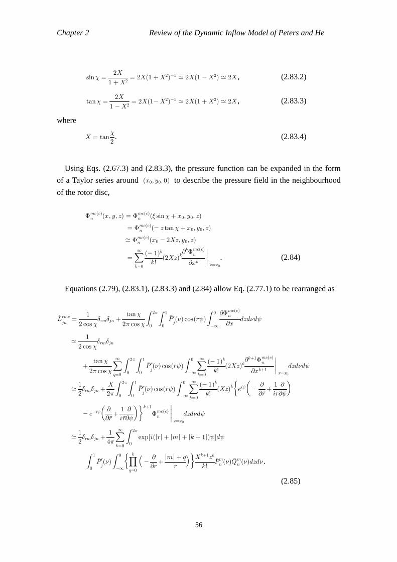
Chapter 2 Review of the Dynamic Inflow Model of Peters and He
56
sin1 =1 +X2
2X= 2X(1 +X2)1 ≃ 2X(1 X2) ≃ 2X, (2.83.2)
tan1 =1 X2
2X= 2X(1X2)1 ≃ 2X(1 +X2) ≃ 2X, (2.83.3)
where
X = tan2
1. (2.83.4)
Using Eqs. (2.67.3) and (2.83.3), the pressure function can be expanded in the form
of a Taylor series around (x0, y0, 0) to describe the pressure field in the neighbourhood
of the rotor disc,
Φmc(c)n (x, y, z) = Φmc(c)n ($ sin1+ x0, y0, z)
= Φmc(c)n ( z tan1+ x0, y0, z) ≃ Φmc(c)n (x0 2Xz, y0, z)
=∑
k=0
∞
k!
( 1)k(2Xz)k
∂xk
∂kΦmc(c)n
x=x0
. (2.84)
Equations (2.79), (2.83.1), (2.83.3) and (2.84) allow Eq. (2.77.1) to be rearranged as
L rmcjn
=2 cos 1
1<rm<jn +
22 cos 1
tan1∫
0
22∫
0
1
Prj() cos(rψ)
∫
∞
0
∂x
∂Φmc(c)ndzddψ
≃2 cos 1
1<rm<jn
+22 cos 1
tan1 ∑
q=0
∞ ∫
0
22∫
0
1
Prj() cos(rψ)
∫
∞
0 ∑
k=0
∞
k!
( 1)k(2Xz)k
∂xk+1
∂k+1Φmc(c)n
x=x0
dzddψ
≃2
1<rm<jn +
22
X∫
0
22∫
0
1
Prj() cos(rψ)
∫
∞
0 ∑
k=0
∞
k!
( 1)k(Xz)k
eiψ
∂r
∂+ir
1
∂ψ
∂
eiψ
∂r
∂+ir
1
∂ψ
∂
k+1
Φmc(c)n
x=x0
dzddψ
≃2
1<rm<jn +
42
1 ∑
k=0
∞ ∫
0
22
exp[i(|r| + |m| + |k + 1|)ψ]dψ
∫
0
1
Prj()
∫
∞
0∏
q=0
k
∂r
∂+
r
|m| + q
k!
Xk+1zkPmn ()Q
mn ()dzd .
(2.85)
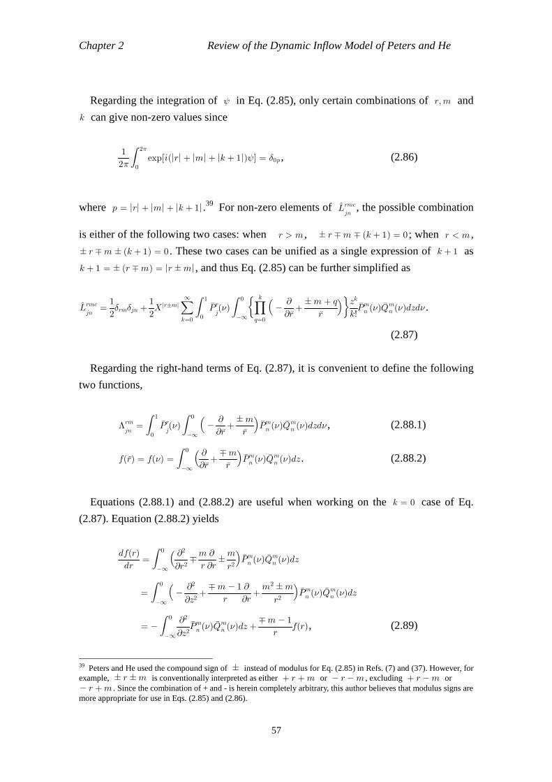
Chapter 2 Review of the Dynamic Inflow Model of Peters and He
57
Regarding the integration of ψ in Eq. (2.85), only certain combinations of r, m and
k can give non-zero values since
22
1∫
0
22
exp[i(|r| + |m| + |k + 1|)ψ] = <0p , (2.86)
where p = |r| + |m| + |k + 1| .39 For non-zero elements of L rmcjn
, the possible combination
is either of the following two cases: when r > m , r m (k + 1) = 0 ; when r < m ,
r m (k + 1) = 0 . These two cases can be unified as a single expression of k + 1 as
k + 1 = (r m) = |r m| , and thus Eq. (2.85) can be further simplified as
L rmcjn
=2
1<rm<jn +
2
1X|rm|
∑
k=0
∞ ∫
0
1
Prj()
∫
∞
0∏
q=0
k
∂r
∂+
r
m + q
k!
zkPmn ()Q
mn ()dzd .
(2.87)
Regarding the right-hand terms of Eq. (2.87), it is convenient to define the following
two functions,
Λrmjn=
∫
0
1
Prj()
∫
∞
0
∂r
∂+
r
mPmn ()Q
mn ()dzd , (2.88.1)
f(r) = f() =
∫
∞
0
∂r
∂+
r
mPmn ()Q
mn ()dz. (2.88.2)
Equations (2.88.1) and (2.88.2) are useful when working on the k = 0 case of Eq.
(2.87). Equation (2.88.2) yields
dr
df(r)=
∫
∞
0
∂r2∂2
r
m
∂r
∂ r2m
Pmn ()Qmn ()dz
=∫
∞
0
∂z2∂2+
r
m 1∂r
∂+
r2m2 m
Pmn ()Qmn ()dz
= ∫
∞
0
∂z2∂2Pmn ()Q
mn ()dz + r
m 1f(r), (2.89)
39 Peters and He used the compound sign of instead of modulus for Eq. (2.85) in Refs. (7) and (37). However, for example, r m is conventionally interpreted as either + r +m or r m , excluding + r m or r +m . Since the combination of + and - is herein completely arbitrary, this author believes that modulus signs are more appropriate for use in Eqs. (2.85) and (2.86).
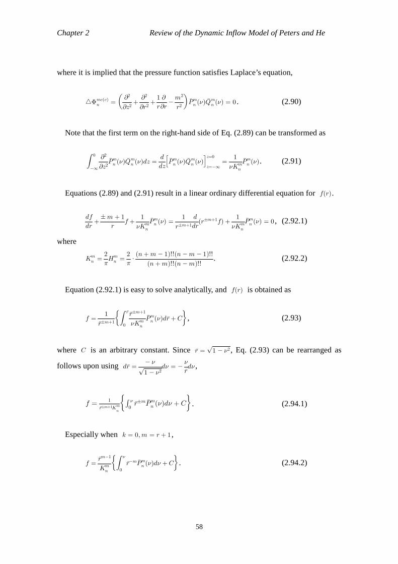
Chapter 2 Review of the Dynamic Inflow Model of Peters and He
58
where it is implied that the pressure function satisfies Laplace’s equation,
Φmc(c)n =
∂z2∂2+∂r2∂2+r
1
∂r
∂ r2m2
Pmn ()Qmn () = 0 . (2.90)
Note that the first term on the right-hand side of Eq. (2.89) can be transformed as
∫
∞
0
∂z2∂2Pmn ()Q
mn ()dz = dz
d[
Pmn ()Qmn ()
]z=0
z=∞=Kmn
1Pmn (). (2.91)
Equations (2.89) and (2.91) result in a linear ordinary differential equation for f(r).
dr
df+
r
m + 1f +
Kmn
1Pmn () = rm+1
1
dr
d(rm+1f) +
Kmn
1Pmn () = 0 , (2.92.1)
where
Kmn = 2
2Hmn = 2
2 (n +m)!!(n m)!!
(n +m 1)!!(n m 1)!!. (2.92.2)
Equation (2.92.1) is easy to solve analytically, and f(r) is obtained as
f =rm+11∫
0
r
Kmn
rm+1Pmn ()dr+ C
, (2.93)
where C is an arbitrary constant. Since r= 1 2√
, Eq. (2.93) can be rearranged as
follows upon using dr =1 2
√
d = r
d ,
f =rm+1Km
n
1
∫
0
rmPmn ()d + C
. (2.94.1)
Especially when k = 0, m = r + 1 ,
f =Kmn
rm1∫
0
rmPmn ()d + C
. (2.94.2)
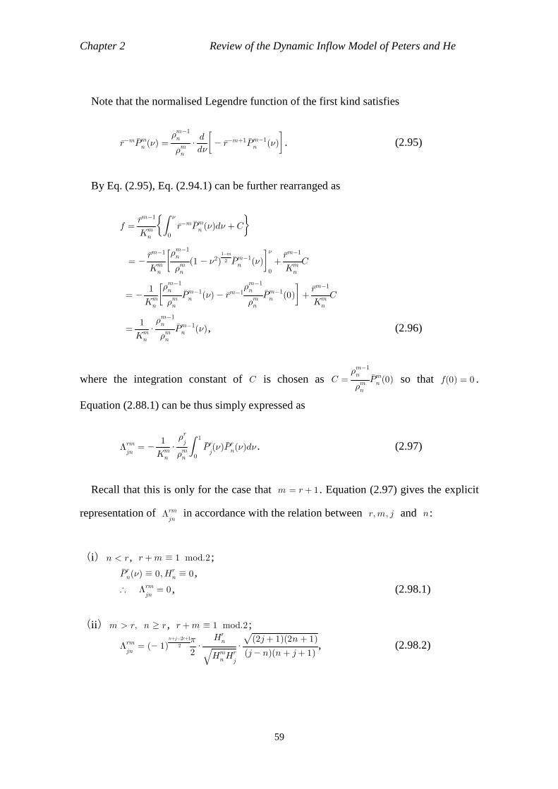
Chapter 2 Review of the Dynamic Inflow Model of Peters and He
59
Note that the normalised Legendre function of the first kind satisfies
rmPmn () = mn
m1n
d
d
rm+1Pm1n ()
. (2.95)
By Eq. (2.95), Eq. (2.94.1) can be further rearranged as
f =Kmn
rm1∫
0
rmPmn ()d + C
= Kmn
rm1
mn
m1n
(1 2) 2
1mPm1n ()
0
+Kmn
rm1C
= Kmn
1
mn
m1n
Pm1n () rm1
mn
m1n
Pm1n (0)
+Kmn
rm1C
=Kmn
1 mn
m1n
Pm1n (), (2.96)
where the integration constant of C is chosen as C =mn
m1nPmn (0) so that f(0) = 0 .
Equation (2.88.1) can be thus simply expressed as
Λrmjn=
Kmn
1 mn
rj∫
0
1
Prj()Prn()d . (2.97)
Recall that this is only for the case that m = r+ 1 . Equation (2.97) gives the explicit
representation of Λrmjn
in accordance with the relation between r,m, j and n:
(i)n < r, r +m 1 mod.2 ; Prn() 0, Hr
n 0 ,
∴ Λrmjn= 0 , (2.98.1)
(ii)m > r, n r, r +m 1 mod.2 ;
Λrmjn= ( 1) 2
n+j2r+1
2
2 HmnH
r
j
√
Hrn (j n)(n + j+ 1)(2j+ 1)(2n + 1)
√
, (2.98.2)
Chapter 2 Review of the Dynamic Inflow Model of Peters and He
60
(iii)n r, m > r, r +m 0 mod.2 ;
Λrmjn= <jn
Hmn
Hrn
√√√√ , (2.98.3)
(iv)n < r, m > r, r +m 0 mod.2 ;
Λrmjn= ( 1) 2
n+j2r
HmnH
r
j
√1
(n + r)!!(r n 1)!!(n + r 1)!!(r n 2)!!
(j n)(n + j+ 1)(2j+ 1)(2n + 1)
√
.
(2.98.4)
2.2.12 The Gain Matrix, L - part 5 -The Elements in Closed Forms
Using the results of the previous Subsection, the integrals of Eqs. (2.66.1) - (2.66.3)
can be explicitly represented in the following forms(7),
[L 0mjn]c = (Xm)[Γ0m
jn] , (2.99.1)
[L rmjn]c = [X|rm| + ( 1)min(r,m)X|r+m|][Γrm
jn] , (2.99.2)
[L rmjn]s = [X|rm| ( 1)min(r,m)X|r+m|][Γrm
jn] , (2.99.3)
where Γ is a function defined as follows,
Γrmjn=∑
l=r+1
∞ArjlΛrmln
. (2.100)
Note that Γ takes different values depending on whether r +m is odd or even
(i) r +m 0 mod.2 ;
Γrmjn=
Hmn
Hrn
√√√√
∑
l=r+1
∞ ∫
0
1
ArjlPrl()Prn()d
=Hmn
Hrn
√√√√
∫
0
1
Prj()Prn()d
Chapter 2 Review of the Dynamic Inflow Model of Peters and He
61
=Hmn
Hrn
√√√√ Ar
jn
=HmnH
r
j
√( 1) 2
n+j2r
(n + j)(n + j+ 2)[(n j)2 1]
2 (2n + 1)(2j+ 1)√
, (2.101.1)
(ii) r +m 0 mod.1 , j = n 1 ;
Γrmjn= sgn(r m)
2
2 Hmn
Hrn
√√√√
∑
l=r+1
∞ ∫
0
1
ArjlPrl()Prn()d
= sgn(r m)2
2 Hmn
Hrn
√√√√
∫
0
1
Prj()Prn()d
= sgn(r m)2
2 Hmn
Hrn
√√√√
(2n + 3)(2n + 1)
(n + 1 + r)(n + 1 r)√
∫
0
1
Prj()Pr
n+1()
+(2n + 1)(2n 1)(n 1)(n + r)
√∫
0
1
Prj()Pr
n1()d
= sgn(r m)2
2 Hmn
Hrn
√√√√
Hr
n+1
1√
(2n + 1)(2n + 3)√
1<j,n+1
+Hrn1
1√
(2n + 1)(2n 1)√
1<j,n1
=2 Hm
nHr
j
√
2 (2n + 1)(2j+ 1)
√sgn(r m)
<j,n1 , (2.101.2)
(iii) r +m 1 mod.2 , j =n 1 ;
Γrmjn= 0 . (2.101.3)
Note that Eqs. (2.101.1) - (2.101.3) indicate that every other element of the gain
matrix, whether moving along a row or a column, is zero (i.e. the matrix looks like a
chessboard). Note also that the only variable of the gain matrix is the wake skew angle,
1. Some specific examples of Eqs. (2.101.1) - (2.101.3) are shown below, using both 1
Chapter 2 Review of the Dynamic Inflow Model of Peters and He
62
and :e40,
L00c11=2
3, (2.102.1)
L 01c12=
10√22 tan
2
1=
10√22
1 + sin:e
1 sin:e√
, (2.102.2)
L 10c21=
10√22 tan
2
1=
10√22
1 + sin:e
1 sin:e√
, (2.102.3)
L 11s22=4
5
1 + tan22
1
=2(1 + sin:e)
5 , (2.102.4)
L 11c22=4
5
1 tan22
1
=2(1 + sin:e)
5 sin:e , (2.102.5)
where the following trigonometric formulae are used.
tan22
1=1 + cos 1
1 cos 1=1 + sin:e
1 sin:e, (2.103.1)
1 + tan22
1=1 + cos 1
2=1 + sin:e
2 , (2.103.2)
1 tan22
1=1 + cos 1
2 cos 1=1 + sin:e
2 sin:e . (2.103.3)
The simplest example of the gain matrix is a 3 3 matrix for the three-state model,
which comprised only those elements in which r = 0, m is either 0 or 1 depending
on r +m mod.2 , and j = r + 1, n = m + 1 .
M00
110 0
0 M11
220
0 0 M11
22
a 0c1
b 1s2
a 1c2
+
L00c11
0 L01c12
0 L11s22
0
L10c21
0 L11c22
1
V
a0c1
b1s2
a1c2
=
A0c(t)1
A1s(t)2
A1c(t)2
+
A0c(c)1
A1s(c)2
A1c(c)2
=
A0c1
A1s2
A1c2
.
(2.104)
40 In Ref. (28), the effective angle of attack, :e = 22 1= tan1
@
?, is used instead of 1 in the representation of
the gain matrix. Unless reference is made to Eqs. (2.103.1) - (2.103.3), it may appear that the gain matrix for Chen’s model has quite different entries from those in which the wake skew angle is used. He also recommended in Ref. (7) that the effective angle of attack should be used instead of the wake skew angle in relation to Peters and HaQuang’s non-linear model, but the reason is not therein stated. This author believes that the difference is not mathematically essential so far as Eqs. (2.103.1) - (2.103.3) are valid.
Chapter 2 Review of the Dynamic Inflow Model of Peters and He
63
In Eq. (2.104), A0c1, A1s2
and A1c2
should be associated with an appropriate lift theory.
References (7), (37), (92) and (112) describe some examples of the possible lift theories.
2.3 The Pitt and Peters model The Pitt and Peters model(1) is a predecessor to the Peters and He model, but is still
arguably one of the most popular dynamic inflow models widely used today. Although
these two models look similar at a glance, the mathematical derivation and the resultant
matrices are quite different, and the relation between these two models has not been
fully explained in the pertinent literature. Reference (101) should be a rare reference
which shows that the Pitt and Peter model forms a special case of the Peters and He
model for axial flight cases, but for other flight scenarios between these two models has
not been fully theoretically elucidated, and the correlation was shown only
experimentally41.
In this Section, the relation between the Pitt and Peters model and the Peters and He
model shall be theoretically examined aiming to make clear the connection between the
two models.
2.3.1 The Apparent Mass Matrix, M
The main difference between the two models lies in the fact that while in the Peters
and He model the induced flow is associated with lift coefficients, Amn , in the Pitt and
Peters model, the induced flow is associated with rotor loadings, CT, CM and CL.
The thrust coefficient is defined as
CT ∫∫
ΦdA&=0,= 1r2
√ , (2.105)
where
Φ(, &, ψ, t) =∑
m=0
∞ ∑
n=m+1,m+3,...
∞Pmn ()Q
mn (i&)
[
Cmn (t) cos(mψ) +Dmn (t) sin(mψ)
]
.
(2.106)
Since those terms in which m =0 will be zero when integrated over [0, 22] with
respect to ψ , Eq. (2.105) simply results in
41 The Pitt and Peters model was seldom theoretically compared with the Peters and He model, in a published paper available, despite other wake models were compared with the Peters and He model to validate the model(92). In fact, References (63) and (101) are only references, to the best knowledge of the present author, in which the relationship between these two models is discussed. However, the discussion is limited to an experimental result, and the mathematical relationship is not clarified at all.
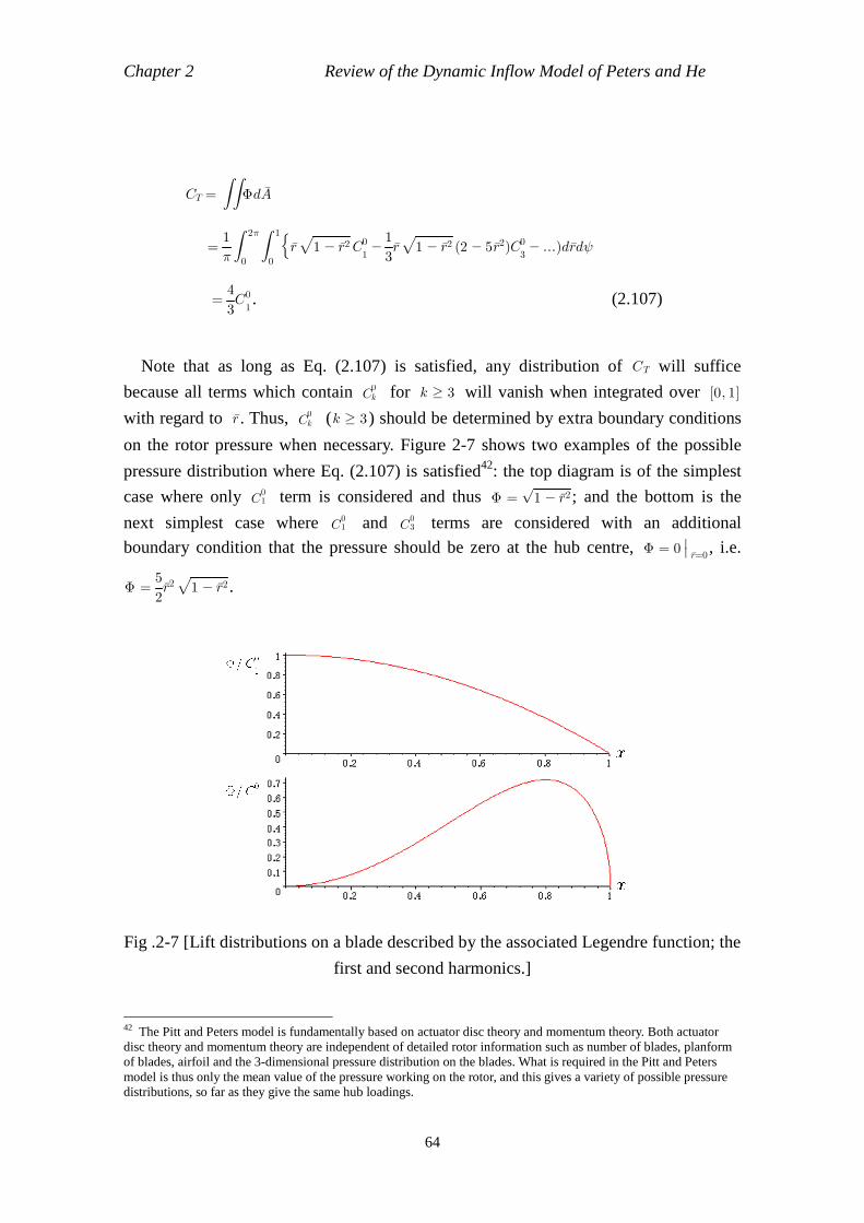
Chapter 2 Review of the Dynamic Inflow Model of Peters and He
64
CT =
∫∫
ΦdA
=2
1∫
0
22∫
0
1
r 1 r2√
C013
1r 1 r2√
(2 5r2)C03 ...)drdψ
=3
4C01. (2.107)
Note that as long as Eq. (2.107) is satisfied, any distribution of CT will suffice
because all terms which contain C0k for k 3 will vanish when integrated over [0, 1]
with regard to r. Thus, C0k (k 3) should be determined by extra boundary conditions
on the rotor pressure when necessary. Figure 2-7 shows two examples of the possible
pressure distribution where Eq. (2.107) is satisfied42: the top diagram is of the simplest
case where only C01 term is considered and thus Φ = 1 r2√
; and the bottom is the
next simplest case where C01 and C03 terms are considered with an additional
boundary condition that the pressure should be zero at the hub centre, Φ = 0r=0
, i.e.
Φ =2
5r2 1 r2√
.
Fig .2-7 [Lift distributions on a blade described by the associated Legendre function; the
first and second harmonics.]
42 The Pitt and Peters model is fundamentally based on actuator disc theory and momentum theory. Both actuator disc theory and momentum theory are independent of detailed rotor information such as number of blades, planform of blades, airfoil and the 3-dimensional pressure distribution on the blades. What is required in the Pitt and Peters model is thus only the mean value of the pressure working on the rotor, and this gives a variety of possible pressure distributions, so far as they give the same hub loadings.
Chapter 2 Review of the Dynamic Inflow Model of Peters and He
65
On the other hand, CT is related to Amn as follows,
CT 2
1∫
A
LdA =2
1∫
0
22∫
0
1
P01()A0c
1(t)rdrdψ
=2
1∫
0
22∫
0
1
3√
r 1 r2√
drdψ A0c1(t)
=3
√2 A0c1 . (2.108)
Regarding the definition of lift coefficients of higher harmonics (i.e. roll and pitch
moments), Mangler suggested the following form(5,48),
L(r, ψ) =2
1C0 + CL sinψ + CM cos ψ + C2L sin 2ψ + C2M cos 2ψ + .
(2.109)
However, Peters did not mention in the literature the factor of 1/2 appearing in the
first term. It is thus reasonable to assume that the lift coefficients of Pitt and Peters
model are defined as follows,
L(r, ψ) = C0 + 2(CL sinψ + CM cos ψ + C2L sin 2ψ + C2M cos 2ψ + ).
(2.110)
Note that the difference in the definition is of course minor, having no influence on
results so long appropriate attention is paid to these factors43. Coefficients CL and CM
can be associated with lift coefficients, A1s2
and A1c2
, respectively44,
43 Reference (37) does not have a clear definition of lift coefficients, while Reference (1) has a typographical error in the calculation of the lift coefficients. At least in those studies of Peters that appear in the bibliography of this thesis, the lift coefficients are not explicitly defined. There are some other variations in the definition(27)(86), and this situation should confuse readers. 44 Higher harmonics can be defined and determined in the same manner when required. Examples include
C2L 2
1∫
A
L( r2 sin 2Ψ)dA 105
√8 A2s3(t) and C2M
21∫
A
L( r2 cos 2Ψ)dA =105
√8 A2c3(t).
Chapter 2 Review of the Dynamic Inflow Model of Peters and He
66
CL 2
4∫
A
L(r, ψ)( rsinψ)dA
= 2
4∫
0
22∫
0
1
P12()A1s
2(t)r2 sin2ψdrdψ
= 15
√8 A1s2(t), (2.111)
CM 2
4∫
A
L(r, ψ)( rcos ψ)dA
= 2
4∫
0
22∫
0
1
P12()A1c
2(t)r2 cos2ψdrdψ
= 15
√8 A1c2(t). (2.112)
In the Pitt and Peters model, the induced flow is also considered in the following
form,
w = ?0 + ?1sr sinψ + ?1cr cos ψ + ?2sr2 sin 2ψ + ?2cr
2 cos 2ψ + .
(2.113)
Equating Eqs. (2.113), (2.22) and Eq. (2.36) yields
?0 2
1∫
A
wdA = 3√
:01(t), (2.114)
?1s 2
4∫
A
w(rsinψ)dA = 2 15√
;12(t), (2.115)
?1c 2
4∫
A
w(rsinψ)dA = 2 15√
:12(t). (2.116)
Thus,
2
40 0
032
80
0 032
8
a 0c1
b 1s2
a 1cs
=
A0c(t)1
A1s(t)2
A1c(t)s
⇔32
80 0
0452
160
0 0452
16
? 0? s1? c1
=CTCLCM
.
(2.117)
Chapter 2 Review of the Dynamic Inflow Model of Peters and He
67
The matrix appearing on the right-hand side of Eq. (2.117) is well-known as the
apparent mass matrix in the Pitt and Peters model(1)45. It is thus confirmed that the
apparent mass matrix in the Pitt and Peters model is consistently and hierarchically
implied as a special case of the Peters and He model.
2.3.2 The Gain Matrix, L
For the gain matrix, Eq. (2.25) is assumed to represent the inflow distribution in the previous discussion. For a special flight case where
∂t∂= 0 (steady) and z = $ (axial
flight), Eq. (2.15) results in a simple forms,
Φ(t) = 0 , (2.118)
Φ = Φ(c) , (2.119)
w V
1∫
∞
0
∂z
∂Φ(c)d$ =
V
1Φ&=0
. (2.120)
From Eqs. (2.6.1) and (2.120),
?0 =2
1∫
0
22∫
0
1
wrdrdψ
=22V
1∫
0
22∫
0
1∑
m=0
∞ ∑
n=m+1,m+3,...
∞Pmn ()Q
mn (0)
[
Amccn (t) cos(mψ) + Amscn (t) sin(mψ)
rdrdψ
=V
1∫
0
1 ∑
n=1,3,5,...
∞P0n()rdr =
0c(c)n (t). (2.121)
Especially for n = 1 ,
?0 =V
1∫
0
1
P1()rdr A0c(c)1(t) =
2V
1 =0c(c)1
. (2.122)
Indeed, the proportionality coefficient obtained from Eq. (2.122), 1/2 , agrees with
the L11 entry of the gain matrix in the Pitt and Peters model. This result also agrees
with the relation between CT, VT (the non-dimensionalised total flow at the rotor
plane) and ?0 for a steady axial flight case, in which they can be simply obtained from momentum theory, Eq. (2.123), if replacing V and =0c(c)
1 in Eq. (2.122) with VT and
CT, respectively, 45 In some references such as Ref. (107), a matrix having 16/452 for the (2, 2) and (3, 3) entries is introduced as the apparent mass matrix of the Pitt and Peters model. This difference in the sign is caused by a difference in the definitions of CL and CM .
Chapter 2 Review of the Dynamic Inflow Model of Peters and He
68
CT = 2VT?0 , (2.123)
This is not an unexpected coincidence because steady axial flight is presupposed in
the Pitt and Peters model to determine the L11 entry. However, the L11 entry of the
gain matrix obtained from Eq. (2.122) should not be adopted as it is in the unified
model, because the induced flow in Eq. (2.122) is represented by the Fourier coefficient
of = , which is different from : and ; in the previous Subsection.
In Ref. (1), the Pitt and Peters model was derived by determining each element of the
apparent mass and gain matrices by presupposing a specialised flight case, such as
steady axial or edgewise flight. Those entries are collected together into the matrices at
the final stage(1), but the necessary transformation for unifying the model (recall
Subsection 2.2.6) is arguably lacking in the derivation, resulting in a model in which
vectors (:, ;) and (=, ) are mixedly used to represent the same induced flow
distribution.
Whereas some flight cases which are dominated by either Φ(c) or Φ(t) alone (i.e.
only one of (:, ;) or (=, ) is therein dominant and the other is negligible) may be
practically described well by the Pitt and Peters model, this author therefore doubts for
the reason above that there is a problem with the representation of the inflow
components in the Pitt and Peters model.
2.4 The Mass-flow Parameter and Non-linear Versions The flow parameter in the Peters and He model, V , can be the non-dimensionalised
freestream speed, V∞. However, it is better to account for energy added to the flow
from the rotor in order to describe the induced flow in the wake, and Ref. (1)
recommends to replace V with the mass-flow parameter, Vm, which is defined as
Vm =@2 + ?2
√
@2 + ?(? + ?m)=
VT
@2 + ?(? + ?m), (2.124)
where @, ? and ?m are advance ratio, the total inflow, inflow due to the rotor thrust,
respectively. Figure 2-8 shows the relation between these parameters.

Chapter 2 Review of the Dynamic Inflow Model of Peters and He
69
Fig. 2-8 [Inflow components in the wind axes.]
Note that these parameters are defined in the wind axes. In Fig. 2-8, ?f is the normal
component of V∞ and satisfies
? = ?f + ?m. (2.125)
In a steady case, ?m is simply given by momentum theory and is equal to the
uniform component of the induced flow(1,92),
?m =2VT
CT= ?0 . (2.126)
However, in an unsteady case, ?m does not generally coincides with ?0, and is
defined by the first row of the gain matrix as(107)
?m =2
1(1, 0, 0)
[
L
]1 ?0?1s?1c
)
. (2.127)
With regard to the flow parameter, Peters and HaQuang proposed an extended
version for the Pitt and Peters model(107), which is obtained by the following process:
i. swapping the flow parameter, V , with the mass-flow parameter matrix,
V →VT 0 00 Vm 00 0 Vm
; (2.128)
ii. treating all variables as total flow rather than perturbation.
Due to the non-linearity between the mass-flow parameters and inflow components,
this model is called the non-linear version of the Pitt and Peters model or Peters and
Chapter 2 Review of the Dynamic Inflow Model of Peters and He
70
HaQuang’s non-linear model.
This modification should give a better description of induced flow, because the thrust
is more directly related to the total inflow and the induced velocity based on momentum
theory than the roll and pitch moments are. The roll and pitch moments are more
sensitive to the variation in the inflow, and this is indeed the case with this formulation46.
The process (ii) above is done by integrating the perturbation version of Pitt and Peters
model over the rotor disc.
The Peters and He model can also be extended to its non-linear version by replacing
the flow parameter with the mass-flow parameter matrix, in which ?m is defined as
?m =3
√2 (1, 0, 0, ..., 0)[
L rmcjn
]1amn
. (2.129)
This relation can be derived from Eq. (2.108), (2.126) and
?0 ≃ 3√
a01 (2.130)
where a0
1 is the steady uniform induced flow(1,7). This approximation is introduced in
Ref. (7). The non-linear version of Pitt and Peters model is verified in Refs. (62) and
(102). The non-linear version of the Peters and He model is verified in Refs. (7), (92)
and (112) and is widely used today.
The present author has no objection to the validity of those non-linear models at all,
but is of the personal opinion that the naming of “non-linear” might be misleading; in
the context of fluid mechanics, the term of non-linearity is usually associated with the
convection term in the Euler equations or the Navier-Stokes equations. The non-linear
dynamic inflow models are not fully non-linear in this sense, because the derivation of
the model essentially depends on the linearised Euler equations. (The process of
non-linearisation is always a process of deleting infinitesimal variables of higher orders,
and it is impossible to recover those deleted terms at a later stage.) The non-linearity in
the non-linear dynamic inflow models indicates only the non-linear relationships
46 Reference (71) discusses in its Section 10-6 why a different flow parameter for rotor moments than that for the rotor thrust is required for unsteady flight cases.
Chapter 2 Review of the Dynamic Inflow Model of Peters and He
71
between flow parameters and rotor forces considering momentum theory, and thus this
appellation may be confusing.
2.5 Discussion In this Chapter, the Peters and He model was thoroughly reviewed in detail. In order
to explore the possibility of applying the dynamic inflow model to autorotative rotors, a
comprehensive examination of the theoretical derivation of the theory from the first
principles is essential together with the consideration of the assumptions therein used.
In the course of examining the derivation of the model, the assumptions upon which
the Peters and He model is based, (A1) - (C2), are clearly identified in this Chapter.
Among these assumptions, the small wake skew angle assumption, (C2), is arguably
the most objectionable because the wake skew angle can be quite large in forward flight,
and indeed, the Peters and He model was intended to be used for a wide range of wake
skew angles from 0 to 90 . Since the assumption forms a fundamental step of the
derivation, this should be considered as a contradiction, and hence lucid explanation
must be made concerning its validity. Unfortunately, the literature suggests no answer to
this contradiction. The present author shall discuss this problem in Chapter 4 in depth.
With reference to past studies, it appears that the present thesis is the first study to
consider the mathematical relation between the Pitt and Peters model and the Peters and
He model. The present Chapter casts some doubt over whether the Peters and He model
hierarchically includes the Pitt and Peters model. It may be premature to make a
conclusive remark about this matter because this is a type of problem which needs to be
concluded through a plural of more concrete proofs by authorities including the original
authors. It is hoped that this thesis would provoke further discussion of this issue.
Chapter 2 Review of the Dynamic Inflow Model of Peters and He
72
2.6 Chapter Summary This Chapter was written with the objective of providing a sound theoretical basis for
the subsequent Chapters of this thesis. Chapters 3 and 4 are essentially based on the
theoretical considerations of this Chapter, and thus it is believed that the objective above
is attained.
This Chapter can be summarised as follows:
1. The derivation of Peters and He model has been thoroughly re-examined;
2. All assumptions which are used in the derivation have been clearly identified;
3. The limitations of these assumptions and possible modifications have been
considered;
4. The Pitt and Peters model has been reviewed in relation to the Peters and He model,
with some doubt cast on the statement in Ref. (102) that the Peters and He model
hierarchically includes the Pitt and Peters model;
5. The logical inconsistency of the small wake skew angle assumption has been
described.
Chapter 3 Dynamic Inflow Modelling for Autorotative Rotors
73
Chapter 3
Dynamic Inflow Modelling for Autorotative Rotors
N.b.) The content of this Chapter is shortened and published as Ref. (168).
3.1 Introduction In the history of the development of dynamic inflow modelling, scant attention has
been paid so far in analysing autorotative rotors. References. (9), (10) and (151) may be
recherché examples in which the Pitt and Peters model is used for rotors in the
windmill-brake state. Still, little theoretical attention as to the applicability of the model
was paid.
Important theoretical attempts recently made to extend the dynamic inflow model
include Refs. (169) and (170), in which the original model was enhanced to cover the
vortex-ring and windmill-brake states. Although Refs. (169) and (170) are mainly
focused on the vortex ring state and its smooth transition in the context of helicopter
applications, such theoretical works should also be of great importance for gyroplane
engineers.
The aim of this Chapter is to identify a necessary modification to the dynamic inflow
model when applied to an autorotative rotor through reviewing the derivation of
dynamic inflow model from the first principles. Whereas the Peters & He or Pitt and
Peters model is kept in mind as a specific example in the following Sections, the
essence of the discussion is not limited to any particular model, but can be applied for
other variations of dynamic inflow models in general. Results of numerical simulations
are also presented to compare the original and modified models.
Chapter 3 Dynamic Inflow Modelling for Autorotative Rotors
74
3.2 The Applicability of the Dynamic Inflow Model to an Autorotative Rotor
3.2.1 Examination on Matrix Elements of Dynamic Inflow Models
There is a major geometric difference between a powered helicopter rotor and an
autorotating rotor:
(D1) the free stream is coming toward an autorotating rotor from below, while
it is coming from above to a rotor in normal working state (see Fig. 2-3).
Although the terms of the normal working state and the windmill-brake state are
already used in Chapter 1 to describe the rotor states of the helicopter and the gyroplane,
they need to be given more strict definitions here; the state in which a rotor is receiving
the incoming flow from below is hereinafter referred to as the windmill-brake state, and
the state in which a rotor is receiving the inflow from above is referred to as the normal
working state following Ref. (5)47. Point (D1) above can be considered as a fundamental
geometric dissimilitude between windmill-brake and normal working states, and how
the difference in the underlying configuration is reflected on the equations of the
dynamic inflow model is to be discussed in this Chapter. As was seen in Chapter 2, the
entire derivation of Peters and He’s dynamic inflow model is highly mathematical and
complicated though, it is not necessary to trace each and every line of the derivation to
examine the applicability of the model for autorotative rotors. What are required to
discuss point (D1) above are only the base equations, viz., the linearised Euler
equations,
∂t
∂q V∇q = ∇Φ, (3.1)
in which the flow components, q , are defined along a streamline coordinate, $ , whose
positive direction is defined to be upstream. The reason why the second term on the
left-hand side has the sign of minus is that the direction of V is defined to be opposite
47 The definition of these geometric attitudes of a rotor towards the inflow should be independent of whether or not the rotor speed is mechanically retained constant. However, the normal working state conventionally implies that the rotor is governed by an engine, and the wind-mill brake state implies that the rotor is not mechanically driven. Indeed, the fact that an autorotative rotor is not mechanically driven is another major difference from an powered helicopter rotor, but the DOF in the rotor speed can be implemented in a mathematical model with regard to blade dynamics (see Fig. 1-2), and thus any change in the rotor speed can be calculated in the loop in a quasi-steady manner. Thus, this thesis does not pay special attention to the extra DOF in the rotor speed of an autorotative rotor.
Chapter 3 Dynamic Inflow Modelling for Autorotative Rotors
75
to the positive direction of $-axis. Since this is the case both for the normal working
and windmill-brake states by definition (see figure 2-2 about this comparison between
two states of a rotor easier), the left hand side of Eq. (3.1) holds the same for both rotor
states in the vector form.
When focusing only on the z-components of Eq. (3.1), it can be noticed that (i) the
direction of lift against the free stream is different as is shown in Fig. 2-2, and (ii) the
direction of the z-axis and the induced flow in the windmill-brake state are opposite to
those in the normal working state. (Figure 2-2 is obtained by re-drawing Fig. 2-3 so that
the rotor plane should be put horizontally and that the free stream should come from the
upper left side of the rotor in the diagram.) The derivation of dynamic inflow models are
based on the z-component of the linearised Euler equation, thus the model for the
windmill-brake state needs to change the signs of both q and Φ in Eq. (3.1). This
leads to the identical form with that for the normal working state, and therefore it can be
ascertained that each element of the matrices in a dynamic inflow model holds the same
both for normal working and windmill-brake states.
Note that the discussion above is not limited only to the Peters and He model, but
also to other models such as the Pitt and Peters model as long as their derivations are
based on the linearised Euler equations.
3.2.2 Definitions of the Wake Skew Angle
In Fig. 2-2, the wake skew angle, 1, is defined as follows for both normal working
and windmill-brake states(37),
1 = tan1?
@((((
((((. (3.2)
Note that although the general matrix representation of a dynamic inflow model
remains the same, the direction of such parameters as : and 1 must be different
because of the difference in the direction of inflow towards the z-axis of the airframe
(see Fig. 2-2).
When applying a dynamic inflow model to the windmill-brake state, it may happen
that one would misinterpret the inflow angle, : , should be in the range from 90o to
180o for the windmill-brake state unless the definition of : is changed. As a matter of
Chapter 3 Dynamic Inflow Modelling for Autorotative Rotors
76
fact, Chen introduced a different definition of 1 from Eq. (3.2) in that it does not have
the modulus(28), and thus according to this definition, the rotor angle of attack, : ,
should be in the range from 90o to 180o for the windmill-brake.
Chen's definition may look versatile at a glance, because the model could be used both
for normal working and windmill-brake states without any changes in the definition so
that angles of 0 1 90 and angles of 90 1 180 therein indicate the normal
working and windmill-brake states, respectively. However, Chen's definition would
entail unfavourable divergences of some gain matrix elements which contain tan(1/2)
to ∞ at 1 = 180 . Still, that 1 equals 180 means axial descent cases in the
windmill-brake state, which is practically quite a possible operational state for
gyroplanes, and thus the unfavourable divergence has been a problem with dynamic
inflow modelling when applying Chen’s formulation to autorotative rotors.
Intuitively, the windmill-brake state can be regarded upside-down to the normal
working state (Fig. 2-2), and thus : and 1 must be defined so as to come in the range
of 0o and 90o for both states. The modulus sign in the definition should not be
dropped off for this reason.
3.2.3 Examination on the Mass-flow Parameter
Now the mass-flow parameter should be examined. The flow parameter V is
recommended to be replaced with Vm in order to account for energy added in the
wake by the rotor(1,7,66,92). The added energy can also be interpreted as the acceleration
of inflow and the contraction of the wake tube in the normal working state. The
mass-flow parameter defined for the normal working state is to be referred to as Vm+
hereinafter,
Vm+ VT+ ?m∂?m
∂VT
=VT
@2 + (?f + ?m)(?f + 2?m)=
@2 + ?2√
@2 + ?(? + ?m), (3.3)
where the definition of ?m is given as Eq. (2.127).
However, the definition of Vm should be changed for the windmill-brake state,
because a rotor in the wind-mill brake state is not adding but receiving energy from the
Chapter 3 Dynamic Inflow Modelling for Autorotative Rotors
77
free stream (this can be interpreted as the deceleration of inflow or the expansion of the
wake tube). This shall be reflected upon the sign of the second term of Eq. (3.3), and so
the mass-flow parameter for the wind-mill brake state should be defined as
Vm VT ?m∂?m
∂VT
=VT
@2 + (?f + ?m)?f=
@2 + ?2√
@2 + ?(? ?m). (3.4)
The Vm defined for the windmill-brake state in this manner is to be referred to as
Vm hereinafter.
In Eqs. (3.3) and (3.4), ? can consistently be defined as
? = ?f + ?m, (3.5)
where ?m < 0 for the windmill-brake state and ?m > 0 for the normal working state.
The difference in the sign of ?m is the reflection of the geometric difference between
the two states. The following equations are intuitively evident from Fig. 2-2,
|?| = |?f| + |?m| , (for the normal working state) (3.6)
|?| = ||?f| |?m|| . (for the windmill-brake state) (3.7)
Note that the difference between Vm+ and Vm is not naturally accommodated in the
definition of Vm because the difference is the reflection of the physical difference in
those two rotor states in terms of the energy flow, and thus this is independent of the
choice of coordinate system48.
3.2.4 Unified form of Vm+ and Vm
The necessity of separating Vm into Vm+ and Vm can be more mathematically
enunciated than the physical and rather intuitive discussion in the previous Subsection.
Differentiating V2T= @2 + ?2 = @2 + (?f + ?m)
2 with respect to ?m yields
48 If the sign of ?m alone is changed, Vm+ and Vm will mutually invert to each other. This can intuitively interpreted as the reflection of the fact that a rotor in the windmill-brake state can be regarded upside-down to a rotor in the normal working state. An error in the definition of ?m would lead to wrongly swapping Vm+ and Vm.
Chapter 3 Dynamic Inflow Modelling for Autorotative Rotors
78
∂?m
∂VT=VT
?= cos 1 (3.8)
for the normal working state. Especially when in high-speed forward flight,
cos 1 ≃ sin: ≃ tan:. (3.9)
Note that tan: should be always positive due to the modulus sign in Eq. (3.2), and
thus ?/VT in Eq. (3.9) is also required to be positive. When in the normal working state,
this is indeed the case because VT > 0 and ? > 0 . However, ? < 0 when in
autorotation. Hence, this further requires that cos 1 should be defined as |?|/VT in
order to be consistent with Eq. (3.2), if it is supposed to cover both the normal working
and windmill-brake states. Indeed, the minus sign on the right-hand side of Eq. (3.4) is
equivalent to the modulus sign in effect.
In fact, Vm+ and Vm can be unified by using modulus sign as
Vm VT ?m∂?m
∂VT=
VT
@2 + ?2 + ?m|?| . (3.10)
Equation (3.10) can consistently be used both in the normal working and
windmill-brake states and is consistent with Eq. (3.2). In Ref. (104), Peters defined
tan: (Eq. (19), p.66) and reads, “: is always positive, whether the flow is from
above or below”. As discussed above, the mass-flow parameter should be defined as Eq.
(3.10) to be consistent with Peters’ own definition of tan: , Eq. (3.2)49. Further
discussion about this issue shall be held in Appendix 3.1.
3.3 Numerical Simulation The difference between Vm+ and Vm came from rather an elementary and intuitive
discussion, but this would appear to be the first time that the difference has been
explicitly highlighted in relation to the dynamic inflow model. The comparison of Vm+
and Vm is conducted by numerical simulation using a generic rotorcraft simulation
code RASCAL at the University of Glasgow, which was already used for some
studies(9,10,151,154,155), and whose validation was evident in Ref. (152). The non-linear
version of Pitt and Peters model is used in the simulation model to describe the induced
49 The mass-flow parameter, Vm , first appeared in Ref. (66) and has been used in dynamic inflow models of Peters. However, its mathematical derivation is not elucidated in published papers.
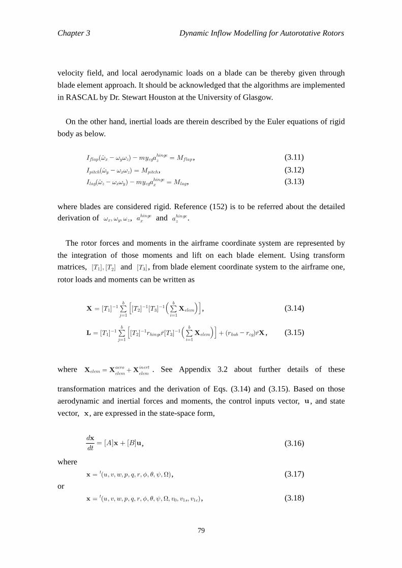
Chapter 3 Dynamic Inflow Modelling for Autorotative Rotors
79
velocity field, and local aerodynamic loads on a blade can be thereby given through
blade element approach. It should be acknowledged that the algorithms are implemented
in RASCAL by Dr. Stewart Houston at the University of Glasgow.
On the other hand, inertial loads are therein described by the Euler equations of rigid
body as below.
Iflap(ω x ωyωz)mycgahingez = Mflap , (3.11)
Ipitch(ω y ωxωz) = Mpitch, (3.12)
Ilag(ω z ωxωy)mycgahingex = Mlag, (3.13)
where blades are considered rigid. Reference (152) is to be referred about the detailed derivation of ωx, ωy, ωz, ahingex and ahingez .
The rotor forces and moments in the airframe coordinate system are represented by
the integration of those moments and lift on each blade element. Using transform
matrices, [T1], [T2] and [T3] , from blade element coordinate system to the airframe one,
rotor loads and moments can be written as
X = [T1]1∑
j=1
b [
[T2]1[T3]
1∑
i=1
b
Xelem
]
, (3.14)
L = [T1]1∑
j=1
b [
[T2]1rhinger[T3]
1∑
i=1
b
Xelem
]
+ (rhub rcg)rX , (3.15)
where Xelem = Xaero
elem+X
inert
elem. See Appendix 3.2 about further details of these
transformation matrices and the derivation of Eqs. (3.14) and (3.15). Based on those
aerodynamic and inertial forces and moments, the control inputs vector, u , and state
vector, x, are expressed in the state-space form,
dt
dx= [A]x + [B]u, (3.16)
where
x = t(u, v, w, p, q, r, B, >, ψ,Ω), (3.17)
or
x = t(u, v, w, p, q, r, B, >, ψ,Ω, v0, v1s, v1c), (3.18)

Chapter 3 Dynamic Inflow Modelling for Autorotative Rotors
80
wherein u =t (<r, &s, &c,Ωp) for gyroplanes50. Note that the model can be linearised
either in the classical 7 DOF rigid-body form with Eq. (3.17) when the inflow dynamics
are effectively treated quasi-statically, or linearised in 10 DOF form with Eq. (3.18) to
encapsulate inflow dynamics. In either case, Eqs. (3.11), (3.12) and (3.13) form a closed
loop together with the dynamic inflow model. (Recall Fig. 1-2.)
Equation (3.16) comprises nearly one hundred non-linear ordinary equations, though
the exact number depends on several parameters including the number of blades. The
set of simultaneous differential equations is to be numerically solved by the
Runge-Kutta method in RASCAL. Further detail about the code can be found in Refs.
(34) and (152). Stability and natural response characteristics of a state described by Eq.
(3.16) can be studied by the eigenvalues of the state matrix, [A] . When the real part of
an eigenvalue is positive, the state (mode) is unstable. Likewise, when negative, then
stable. The imaginary part of an eigenvalue means the modal frequency.
3.4 Results from Numerical Simulation The numerical simulation was computed to see how much the difference between
Vm+ and Vm would influence the induced velocity and flight controls under different
trim conditions. Used therein are two types of rotorcraft: Montgomerie, which is a
two-seater medium gyroplane, and Westland Puma (see Fig. 3-1), which is a much
heavier helicopter. Their brief specifications are shown in Table 3-1.
Fig. 3-1 [Montgomerie (left) and Westland Puma (right).]51
50 It is characteristic to the gyroplane that the propeller speed is in the control inputs vector. 51 The left picture in Fig. 3-1 is reproduced from the webpage of Flight Dynamics Group at Glasgow University. The right picture is kindly provided by AgustaWestland, with copyright approved.
Chapter 3 Dynamic Inflow Modelling for Autorotative Rotors
81
Montgomerie Puma
M (kg)
Ixx (kgm2)
Iyy (kgm2)
Izz (kgm2)
Ixz (kgm2)
b
R (m)
m (kg)
350
73
297
224
0
2
3.81
15
5810
9638
33240
25889
2226
4
7.498
91
Table 3-1 [Specification of the Montgomerie and Puma.]
Since the rotor of a gyroplane is always in the windmill-brake state, simulations for
the Montgomerie were done over a wide range of practical forward flight speeds and
descent rates. On the other hand, the Puma was assumed to be descending with a fixed
collective pitch, which is the most practical case where a helicopter rotor enters the
windmill-brake state, because helicopter rotors usually enter the windmill-brake state
only in emergency situations such as sudden power failure, where collective pitch
should be minimized so as to keep the rotor speed as high as possible.
Figures 3-2 to 3-8 are related to the Montgomerie: Fig. 3-2 shows the resultant
variation between the magnitude of dimensional mass-flow parameters of vm+ and
vm; Fig. 3-3 to 3-8 show the influence of the difference in the mass-flow parameters in
terms of forward flight speed and the descent rate against the inflow components,
airframe attitudes and flight controls in trim, respectively.
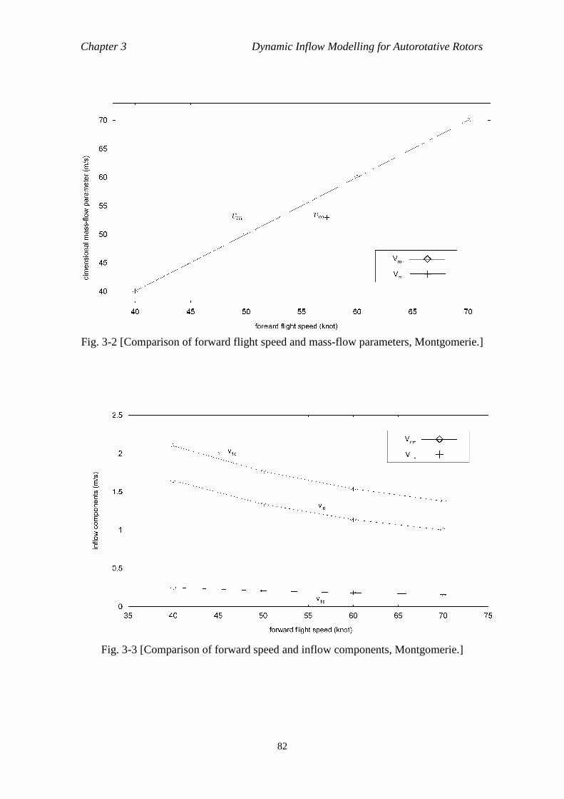
Chapter 3 Dynamic Inflow Modelling for Autorotative Rotors
82
Fig. 3-2 [Comparison of forward flight speed and mass-flow parameters, Montgomerie.]
Fig. 3-3 [Comparison of forward speed and inflow components, Montgomerie.]

Chapter 3 Dynamic Inflow Modelling for Autorotative Rotors
83
Fig. 3-4 [Comparison of forward speed and airframe attitude, Montgomerie.]
Fig. 3-5 [Comparison of descent rate and inflow components
at 50 knots, Montgomerie.]
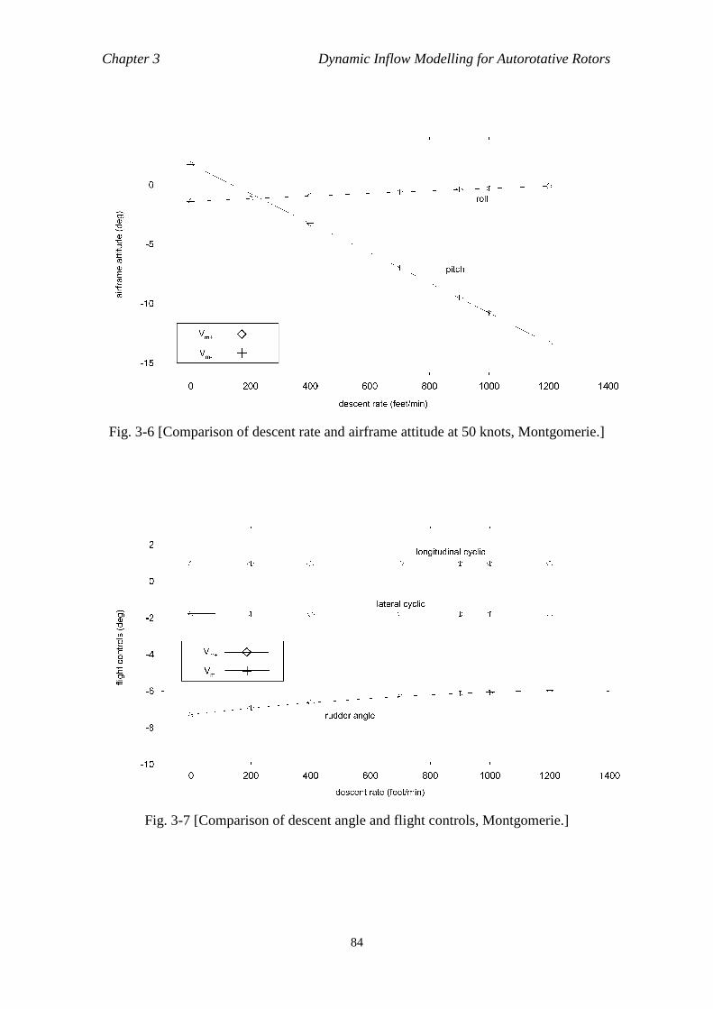
Chapter 3 Dynamic Inflow Modelling for Autorotative Rotors
84
Fig. 3-6 [Comparison of descent rate and airframe attitude at 50 knots, Montgomerie.]
Fig. 3-7 [Comparison of descent angle and flight controls, Montgomerie.]
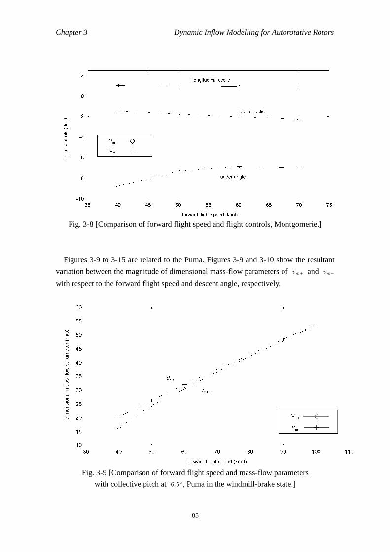
Chapter 3 Dynamic Inflow Modelling for Autorotative Rotors
85
Fig. 3-8 [Comparison of forward flight speed and flight controls, Montgomerie.]
Figures 3-9 to 3-15 are related to the Puma. Figures 3-9 and 3-10 show the resultant
variation between the magnitude of dimensional mass-flow parameters of vm+ and vm
with respect to the forward flight speed and descent angle, respectively.
Fig. 3-9 [Comparison of forward flight speed and mass-flow parameters
with collective pitch at 6.5 , Puma in the windmill-brake state.]
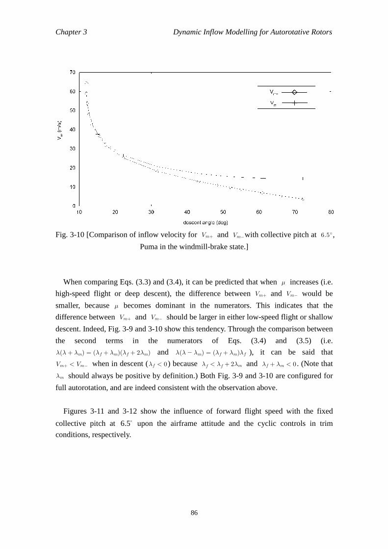
Chapter 3 Dynamic Inflow Modelling for Autorotative Rotors
86
Fig. 3-10 [Comparison of inflow velocity for Vm+ and Vmwith collective pitch at 6.5 ,
Puma in the windmill-brake state.]
When comparing Eqs. (3.3) and (3.4), it can be predicted that when @ increases (i.e.
high-speed flight or deep descent), the difference between Vm+ and Vm would be
smaller, because @ becomes dominant in the numerators. This indicates that the
difference between Vm+ and Vm should be larger in either low-speed flight or shallow
descent. Indeed, Fig. 3-9 and 3-10 show this tendency. Through the comparison between
the second terms in the numerators of Eqs. (3.4) and (3.5) (i.e.
?(? + ?m) = (?f + ?m)(?f + 2?m) and ?(? ?m) = (?f + ?m)?f ), it can be said that
Vm+ < Vm when in descent (?f < 0) because ?f < ?f + 2?m and ?f + ?m < 0 . (Note that
?m should always be positive by definition.) Both Fig. 3-9 and 3-10 are configured for
full autorotation, and are indeed consistent with the observation above.
Figures 3-11 and 3-12 show the influence of forward flight speed with the fixed
collective pitch at 6.5o upon the airframe attitude and the cyclic controls in trim
conditions, respectively.
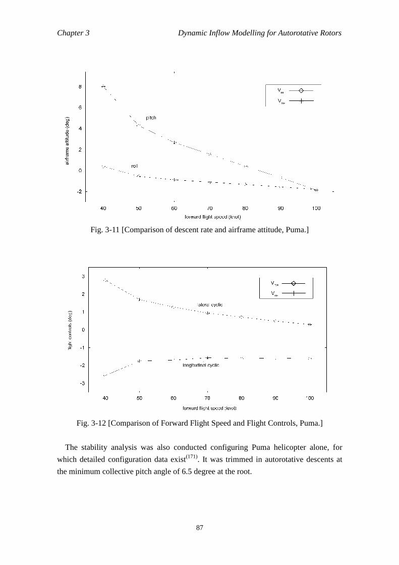
Chapter 3 Dynamic Inflow Modelling for Autorotative Rotors
87
Fig. 3-11 [Comparison of descent rate and airframe attitude, Puma.]
Fig. 3-12 [Comparison of Forward Flight Speed and Flight Controls, Puma.]
The stability analysis was also conducted configuring Puma helicopter alone, for
which detailed configuration data exist(171). It was trimmed in autorotative descents at
the minimum collective pitch angle of 6.5 degree at the root.
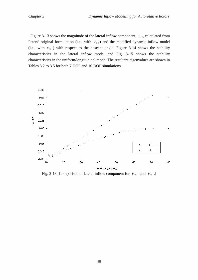
Chapter 3 Dynamic Inflow Modelling for Autorotative Rotors
88
Figure 3-13 shows the magnitude of the lateral inflow component, v1s, calculated from
Peters’ original formulation (i.e., with Vm+) and the modified dynamic inflow model
(i.e., with Vm) with respect to the descent angle. Figure 3-14 shows the stability
characteristics in the lateral inflow mode, and Fig. 3-15 shows the stability
characteristics in the uniform/longitudinal mode. The resultant eigenvalues are shown in
Tables 3.2 to 3.5 for both 7 DOF and 10 DOF simulations.
Fig. 3-13 [Comparison of lateral inflow component for Vm+ and Vm.]

Chapter 3 Dynamic Inflow Modelling for Autorotative Rotors
89
Fig. 3-14 [Lateral inflow mode; comparison for Vm+ and Vm.]
Fig. 3-15 [Coupled uniform/longitudinal inflow modes;
comparison for Vm+ and Vm.]
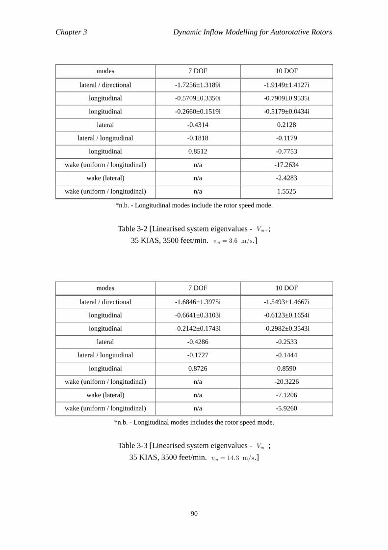
Chapter 3 Dynamic Inflow Modelling for Autorotative Rotors
90
modes 7 DOF 10 DOF
lateral / directional -1.7256±1.3189i -1.9149±1.4127i
longitudinal -0.5709±0.3350i -0.7909±0.9535i
longitudinal -0.2660±0.1519i -0.5179±0.0434i
lateral -0.4314 0.2128
lateral / longitudinal -0.1818 -0.1179
longitudinal 0.8512 -0.7753
wake (uniform / longitudinal) n/a -17.2634
wake (lateral) n/a -2.4283
wake (uniform / longitudinal) n/a 1.5525
*n.b. - Longitudinal modes include the rotor speed mode.
Table 3-2 [Linearised system eigenvalues - Vm+;
35 KIAS, 3500 feet/min. vm = 3.6 m/s.]
modes 7 DOF 10 DOF
lateral / directional -1.6846±1.3975i -1.5493±1.4667i
longitudinal -0.6641±0.3103i -0.6123±0.1654i
longitudinal -0.2142±0.1743i -0.2982±0.3543i
lateral -0.4286 -0.2533
lateral / longitudinal -0.1727 -0.1444
longitudinal 0.8726 0.8590
wake (uniform / longitudinal) n/a -20.3226
wake (lateral) n/a -7.1206
wake (uniform / longitudinal) n/a -5.9260
*n.b. - Longitudinal modes includes the rotor speed mode.
Table 3-3 [Linearised system eigenvalues - Vm;
35 KIAS, 3500 feet/min. vm = 14.3 m/s.]
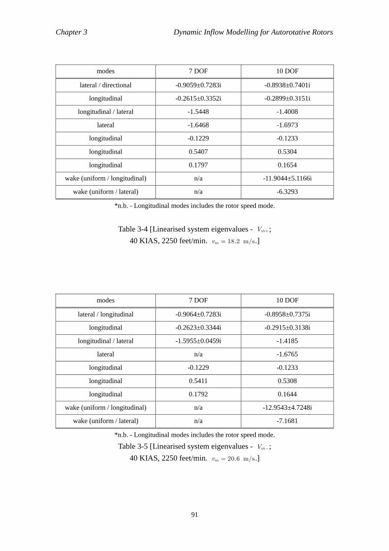
Chapter 3 Dynamic Inflow Modelling for Autorotative Rotors
91
modes 7 DOF 10 DOF
lateral / directional -0.9059±0.7283i -0.8938±0.7401i
longitudinal -0.2615±0.3352i -0.2899±0.3151i
longitudinal / lateral -1.5448 -1.4008
lateral -1.6468 -1.6973
longitudinal -0.1229 -0.1233
longitudinal 0.5407 0.5304
longitudinal 0.1797 0.1654
wake (uniform / longitudinal) n/a -11.9044±5.1166i
wake (uniform / lateral) n/a -6.3293
*n.b. - Longitudinal modes includes the rotor speed mode.
Table 3-4 [Linearised system eigenvalues - Vm+;
40 KIAS, 2250 feet/min. vm = 18.2 m/s.]
modes 7 DOF 10 DOF
lateral / longitudinal -0.9064±0.7283i -0.8958±0.7375i
longitudinal -0.2623±0.3344i -0.2915±0.3138i
longitudinal / lateral -1.5955±0.0459i -1.4185
lateral n/a -1.6765
longitudinal -0.1229 -0.1233
longitudinal 0.5411 0.5308
longitudinal 0.1792 0.1644
wake (uniform / longitudinal) n/a -12.9543±4.7248i
wake (uniform / lateral) n/a -7.1681
*n.b. - Longitudinal modes includes the rotor speed mode.
Table 3-5 [Linearised system eigenvalues - Vm;
40 KIAS, 2250 feet/min. vm = 20.6 m/s.]
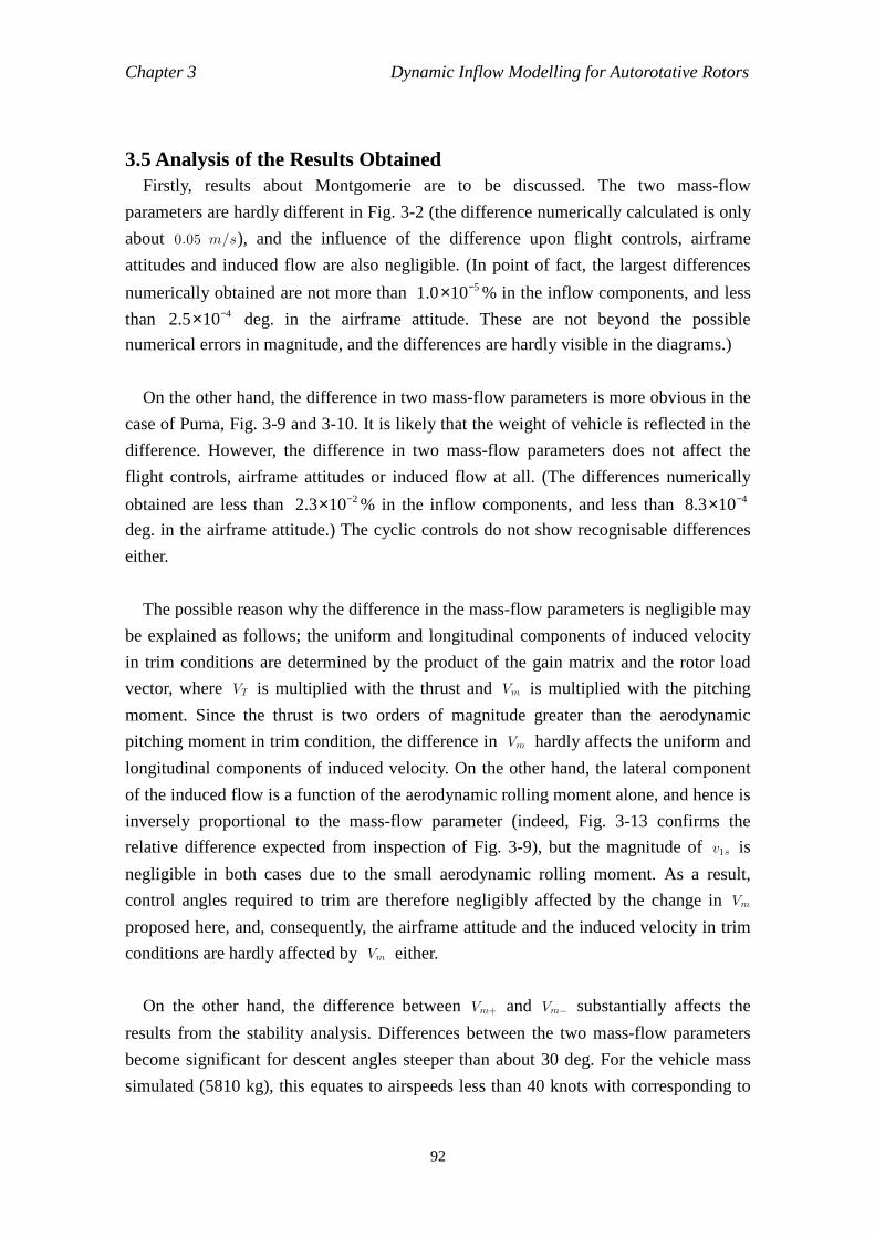
Chapter 3 Dynamic Inflow Modelling for Autorotative Rotors
92
3.5 Analysis of the Results Obtained Firstly, results about Montgomerie are to be discussed. The two mass-flow
parameters are hardly different in Fig. 3-2 (the difference numerically calculated is only
about 0.05 m/s), and the influence of the difference upon flight controls, airframe
attitudes and induced flow are also negligible. (In point of fact, the largest differences
numerically obtained are not more than 51.0 10−× % in the inflow components, and less
than 42.5 10−× deg. in the airframe attitude. These are not beyond the possible
numerical errors in magnitude, and the differences are hardly visible in the diagrams.)
On the other hand, the difference in two mass-flow parameters is more obvious in the
case of Puma, Fig. 3-9 and 3-10. It is likely that the weight of vehicle is reflected in the
difference. However, the difference in two mass-flow parameters does not affect the
flight controls, airframe attitudes or induced flow at all. (The differences numerically
obtained are less than 22.3 10−× % in the inflow components, and less than 48.3 10−×
deg. in the airframe attitude.) The cyclic controls do not show recognisable differences
either.
The possible reason why the difference in the mass-flow parameters is negligible may
be explained as follows; the uniform and longitudinal components of induced velocity
in trim conditions are determined by the product of the gain matrix and the rotor load
vector, where VT is multiplied with the thrust and Vm is multiplied with the pitching
moment. Since the thrust is two orders of magnitude greater than the aerodynamic
pitching moment in trim condition, the difference in Vm hardly affects the uniform and
longitudinal components of induced velocity. On the other hand, the lateral component
of the induced flow is a function of the aerodynamic rolling moment alone, and hence is
inversely proportional to the mass-flow parameter (indeed, Fig. 3-13 confirms the
relative difference expected from inspection of Fig. 3-9), but the magnitude of v1s is
negligible in both cases due to the small aerodynamic rolling moment. As a result,
control angles required to trim are therefore negligibly affected by the change in Vm
proposed here, and, consequently, the airframe attitude and the induced velocity in trim
conditions are hardly affected by Vm either.
On the other hand, the difference between Vm+ and Vm substantially affects the
results from the stability analysis. Differences between the two mass-flow parameters
become significant for descent angles steeper than about 30 deg. For the vehicle mass
simulated (5810 kg), this equates to airspeeds less than 40 knots with corresponding to
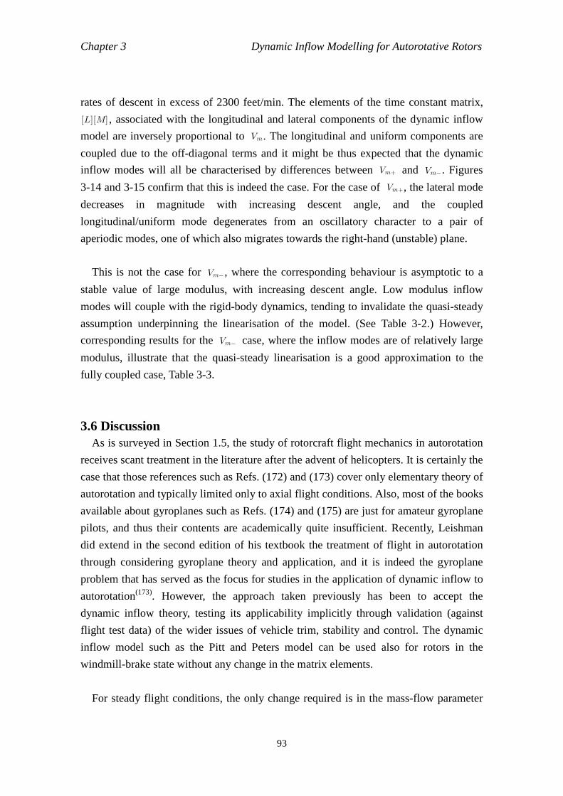
Chapter 3 Dynamic Inflow Modelling for Autorotative Rotors
93
rates of descent in excess of 2300 feet/min. The elements of the time constant matrix,
[L][M] , associated with the longitudinal and lateral components of the dynamic inflow
model are inversely proportional to Vm. The longitudinal and uniform components are
coupled due to the off-diagonal terms and it might be thus expected that the dynamic
inflow modes will all be characterised by differences between Vm+ and Vm. Figures
3-14 and 3-15 confirm that this is indeed the case. For the case of Vm+, the lateral mode
decreases in magnitude with increasing descent angle, and the coupled
longitudinal/uniform mode degenerates from an oscillatory character to a pair of
aperiodic modes, one of which also migrates towards the right-hand (unstable) plane.
This is not the case for Vm, where the corresponding behaviour is asymptotic to a
stable value of large modulus, with increasing descent angle. Low modulus inflow
modes will couple with the rigid-body dynamics, tending to invalidate the quasi-steady
assumption underpinning the linearisation of the model. (See Table 3-2.) However,
corresponding results for the Vm case, where the inflow modes are of relatively large
modulus, illustrate that the quasi-steady linearisation is a good approximation to the
fully coupled case, Table 3-3.
3.6 Discussion As is surveyed in Section 1.5, the study of rotorcraft flight mechanics in autorotation
receives scant treatment in the literature after the advent of helicopters. It is certainly the
case that those references such as Refs. (172) and (173) cover only elementary theory of
autorotation and typically limited only to axial flight conditions. Also, most of the books
available about gyroplanes such as Refs. (174) and (175) are just for amateur gyroplane
pilots, and thus their contents are academically quite insufficient. Recently, Leishman
did extend in the second edition of his textbook the treatment of flight in autorotation
through considering gyroplane theory and application, and it is indeed the gyroplane
problem that has served as the focus for studies in the application of dynamic inflow to
autorotation(173). However, the approach taken previously has been to accept the
dynamic inflow theory, testing its applicability implicitly through validation (against
flight test data) of the wider issues of vehicle trim, stability and control. The dynamic
inflow model such as the Pitt and Peters model can be used also for rotors in the
windmill-brake state without any change in the matrix elements.
For steady flight conditions, the only change required is in the mass-flow parameter
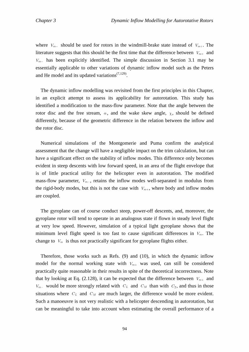
Chapter 3 Dynamic Inflow Modelling for Autorotative Rotors
94
where Vm should be used for rotors in the windmill-brake state instead of Vm+. The
literature suggests that this should be the first time that the difference between Vm+ and
Vm has been explicitly identified. The simple discussion in Section 3.1 may be
essentially applicable to other variations of dynamic inflow model such as the Peters
and He model and its updated variations(7,129).
The dynamic inflow modelling was revisited from the first principles in this Chapter,
in an explicit attempt to assess its applicability for autorotation. This study has
identified a modification to the mass-flow parameter. Note that the angle between the
rotor disc and the free stream, : , and the wake skew angle, 1, should be defined
differently, because of the geometric difference in the relation between the inflow and
the rotor disc.
Numerical simulations of the Montgomerie and Puma confirm the analytical
assessment that the change will have a negligible impact on the trim calculation, but can
have a significant effect on the stability of inflow modes. This difference only becomes
evident in steep descents with low forward speed, in an area of the flight envelope that
is of little practical utility for the helicopter even in autorotation. The modified
mass-flow parameter, Vm, retains the inflow modes well-separated in modulus from
the rigid-body modes, but this is not the case with Vm+, where body and inflow modes
are coupled.
The gyroplane can of course conduct steep, power-off descents, and, moreover, the
gyroplane rotor will tend to operate in an analogous state if flown in steady level flight
at very low speed. However, simulation of a typical light gyroplane shows that the
minimum level flight speed is too fast to cause significant differences in Vm. The
change to Vm is thus not practically significant for gyroplane flights either.
Therefore, those works such as Refs. (9) and (10), in which the dynamic inflow
model for the normal working state with Vm+ was used, can still be considered
practically quite reasonable in their results in spite of the theoretical incorrectness. Note
that by looking at Eq. (2.128), it can be expected that the difference between Vm+ and
Vm would be more strongly related with CL and CM than with CT, and thus in those
situations where CL and CM are much larger, the difference would be more evident.
Such a manoeuvre is not very realistic with a helicopter descending in autorotation, but
can be meaningful to take into account when estimating the overall performance of a
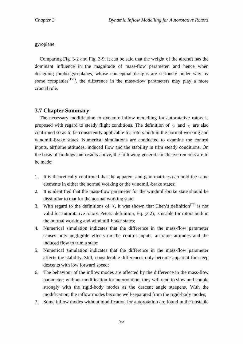
Chapter 3 Dynamic Inflow Modelling for Autorotative Rotors
95
gyroplane.
Comparing Fig. 3-2 and Fig. 3-9, it can be said that the weight of the aircraft has the
dominant influence in the magnitude of mass-flow parameter, and hence when
designing jumbo-gyroplanes, whose conceptual designs are seriously under way by
some companies(157), the difference in the mass-flow parameters may play a more
crucial role.
3.7 Chapter Summary The necessary modification to dynamic inflow modelling for autorotative rotors is
proposed with regard to steady flight conditions. The definition of : and 1 are also
confirmed so as to be consistently applicable for rotors both in the normal working and
windmill-brake states. Numerical simulations are conducted to examine the control
inputs, airframe attitudes, induced flow and the stability in trim steady conditions. On
the basis of findings and results above, the following general conclusive remarks are to
be made:
1. It is theoretically confirmed that the apparent and gain matrices can hold the same
elements in either the normal working or the windmill-brake states;
2. It is identified that the mass-flow parameter for the windmill-brake state should be
dissimilar to that for the normal working state;
3. With regard to the definitions of 1, it was shown that Chen’s definition(28) is not
valid for autorotative rotors. Peters’ definition, Eq. (3.2), is usable for rotors both in
the normal working and windmill-brake states;
4. Numerical simulation indicates that the difference in the mass-flow parameter
causes only negligible effects on the control inputs, airframe attitudes and the
induced flow to trim a state;
5. Numerical simulation indicates that the difference in the mass-flow parameter
affects the stability. Still, considerable differences only become apparent for steep
descents with low forward speed;
6. The behaviour of the inflow modes are affected by the difference in the mass-flow
parameter; without modification for autorotation, they will tend to slow and couple
strongly with the rigid-body modes as the descent angle steepens. With the
modification, the inflow modes become well-separated from the rigid-body modes;
7. Some inflow modes without modification for autorotation are found in the unstable
Chapter 3 Dynamic Inflow Modelling for Autorotative Rotors
96
region. These modes become stable with modification to Vm. The author suggests
that stable modes should be more physically realistic than unstable modes of inflow,
and therefore that Vm should produce more meaningful inflow in autorotation.
8. Due to the limited area of the flight envelope of autorotating rotorcraft where the
modification is practically required, those reference works such as Refs. (9), (10)
and (151), (154) and (155), where unmodified dynamic inflow model is used for
autorotative rotors, can be considered still reasonable about their results.
Chapter 4 Consideration of the Small Wake Skew Angle Assumption
97
Chapter 4
Consideration of the Small Wake Skew Angle Assumption 4.1 Introduction Peters and He derived their dynamic inflow model invariably based on the small
wake skew angle assumption (Subsection 2.2.11), but proceeded to state that this model
can be applied to a wide range of wake skew angles from 0 to 90 (37). Since the model
is extensively compared with experimental data and the correlation is found overall
excellent(7), the practical validity of the model for a wide range of wake skew angles
should be considered acceptable. Still, there is clearly a need to theoretically elucidate
the validity of this approach in the model derivation.
In point of fact, the original authors have never discussed mathematically the validity
of the assumption; indeed the small wake skew angle assumption appears only in the
appendix of Ref. (7) (Appendix C, page 168)52, and the pertinent part of the derivation
is not mentioned in any other relevant published papers.
This author thus believes that the validity of the small wake skew angle assumption
needs to be theoretically re-examined. Note that since the rotor is supposed to be
working in the normal working state in the original works of Peters and He, the normal
working state shall be used as the representative rotor state also in this Chapter.
However, the general coverage of this Chapter shall not be limited to the normal
working state alone.
4.2 New Gain Matrix Model 4.2.1 Derivation of a New No-Assumption Model
In an attempt to examine the small wake skew assumption, a new gain matrix is
proposed without using the assumption. In this formulation, Eqs. (2.77.1) - (2.77.3) are
used instead of Eq. (2.87).
Although all the derivation in Chapter 2 from Eq. (2.77) to (2.104) is applicable to 52 In Ref. (7), the assumption is suddenly introduced with a phrase, “Now we will examine the integral behaviour for small wake skew angle 1 for which we have...” However, it is not analytically explained in any other places why the resultant model can later be extended up to 1 = 2/2 .
Chapter 4 Consideration of the Small Wake Skew Angle Assumption
98
Eqs. (2.77.1) - (2.77.3) except Eqs. (2.83.1) - (2.83.3), the Taylor series of the pressure
potential, Eq. (2.84), should be modified as
Φmc(c)n (x, y, z) = Φmc(c)n (x0 tan1z, y0, z)
=∑
k=0
∞
k!
( 1)k
z tan1
k
∂xk
∂kΦmc(c)n
x=x0
. (4.1)
Note that although it may appear that Eqs. (2.77.1) - (2.77.3) would diverge to
infinity at 1 = 2/2 , this case is already excluded when Eq. (2.69.1) is derived from Eq.
(2.67.3)53. Equations (2.77.1) - (2.77.3) and (4.1) lead to the following final
representations for the new gain matrix elements.
[L 0mjn]c =
cos 1
1(Ym)[Γ0m
jn] , (4.2)
[L rmjn]c =
cos 1
1[Y|rm| + ( 1)min(r,m)Y|r+m|][Γrm
jn] , (4.3)
[L rmjn]s =
cos 1
1[Y|rm| ( 1)min(r,m)Y|r+m|][Γrm
jn] , (4.4)
where
Y =2
tan1. (4.5)
Note that when 1 1 , Eqs. (4.2) - (4.5) reduce to Eqs. (2.99.1) - (2.99.3) and X ,
respectively. Therefore, it can be said that Eqs. (4.2) - (4.5) hierarchically imply Peters
and He’s gain matrix elements for axial flight.
Some examples of Eq. (4.2) - (4.5) are as follows.
L 00c11=2 cos 1
3 , (4.6)
53 Therefore, the extension of the Peters and He model up to edgewise flight is incompatible not only with the small wake skew angle assumption, but also with the derivation of Eq. (2.69.1). This indicates that the edgewise flight case should be discussed separately, if it is possible to deal with analytically. This is indeed the case, and perfectly edgewise flight shall be discussed later in this Chapter.
Chapter 4 Consideration of the Small Wake Skew Angle Assumption
99
L 01c12=
10√
cos 1
2 tan1, (4.7)
L 10c21=
10√
cos 1
2 tan1, (4.8)
L11s22
=2
5
1 +4
1tan2 1
, (4.9)
L11c22
=2
5
1 4
1tan21
. (4.10)
Note also that when 1 1 , Eqs. (4.6) - (4.10) reduce down to Eqs. (2.102.1) -
(2.102.5).
4.2.2 The Modified Pitt and Peters Model
The difference of the gain matrices between the Pitt & Peters and Peters & He models
are only in the coefficients and thus the trigonometric parts are the same54. Thus, it
should be possible to propose a modified Pitt & Peters model as well by replacing the
trigonometric parts in the original Pitt and Peters model with those appearing in Eq.
(4.6) - (4.10). The specific form of the modified model will be as follows;
32
80 0
0 452
160
0 0 452
16
? 0? 1s? 1c
+
2 cos 1
10
64
152 cos 1
tan 1
0 2
1 +4
1tan2 1
0
64
152 cos 1
tan 10 2
1 4
1tan2 1
1
V
1? 0? 1s? 1c
=CTCLCM
(4.11)
For 1 = 0 (hover), Eq. (4.11) is identical with the original Peters and He formulation.
However, with progression into edgewise flight, the (1, 1) element in the gain matrix,
1/2cos1, tends to infinity. This means that the uniform induced velocity will increase
with the wake skew angle, but this is counter to reality. Therefore, despite the derivation
of this model should be mathematically more consistent, it can be predicted that this
model would not provide realistic solutions when 1 is fairly large.
In the next Subsection, numerical simulation of this model is provided.
54 While the Peters and He model is given the general formulation for any combination of m , n , r and j, the Pitt and Peters model is provided only up to the five-state model. Therefore, strictly speaking, the simple replacement in Subsection 4.2.2 can de done only up to the five-state model.
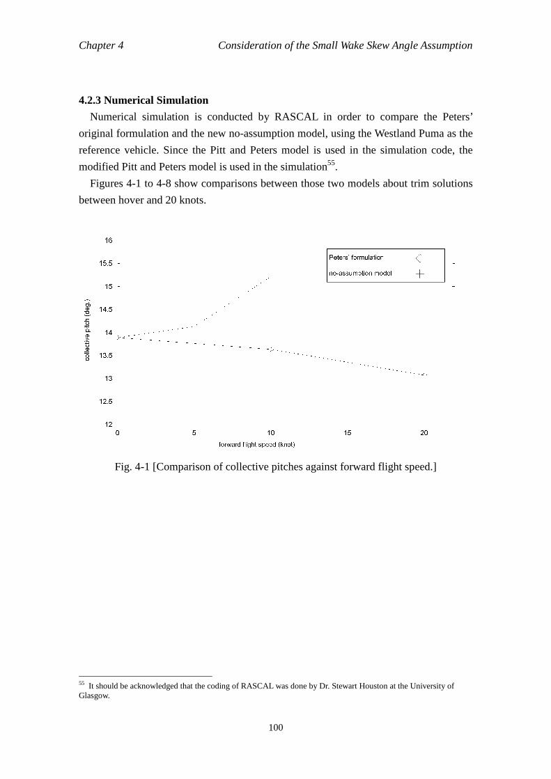
Chapter 4 Consideration of the Small Wake Skew Angle Assumption
100
4.2.3 Numerical Simulation
Numerical simulation is conducted by RASCAL in order to compare the Peters’
original formulation and the new no-assumption model, using the Westland Puma as the
reference vehicle. Since the Pitt and Peters model is used in the simulation code, the
modified Pitt and Peters model is used in the simulation55.
Figures 4-1 to 4-8 show comparisons between those two models about trim solutions
between hover and 20 knots.
Fig. 4-1 [Comparison of collective pitches against forward flight speed.]
55 It should be acknowledged that the coding of RASCAL was done by Dr. Stewart Houston at the University of Glasgow.
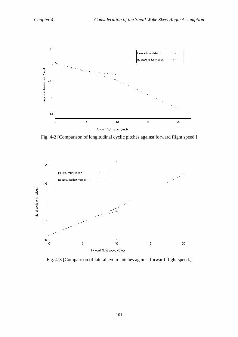
Chapter 4 Consideration of the Small Wake Skew Angle Assumption
101
Fig. 4-2 [Comparison of longitudinal cyclic pitches against forward flight speed.]
Fig. 4-3 [Comparison of lateral cyclic pitches against forward flight speed.]
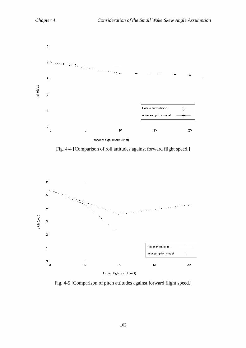
Chapter 4 Consideration of the Small Wake Skew Angle Assumption
102
Fig. 4-4 [Comparison of roll attitudes against forward flight speed.]
Fig. 4-5 [Comparison of pitch attitudes against forward flight speed.]
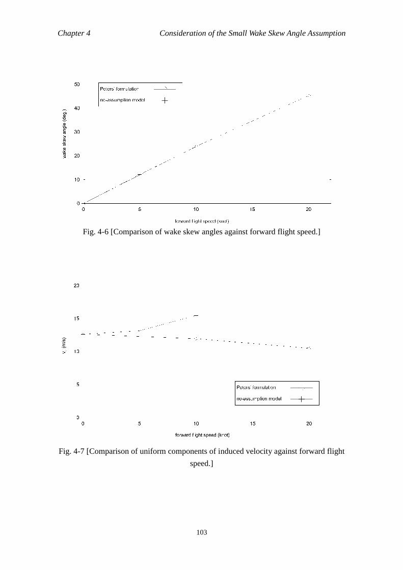
Chapter 4 Consideration of the Small Wake Skew Angle Assumption
103
Fig. 4-6 [Comparison of wake skew angles against forward flight speed.]
Fig. 4-7 [Comparison of uniform components of induced velocity against forward flight
speed.]
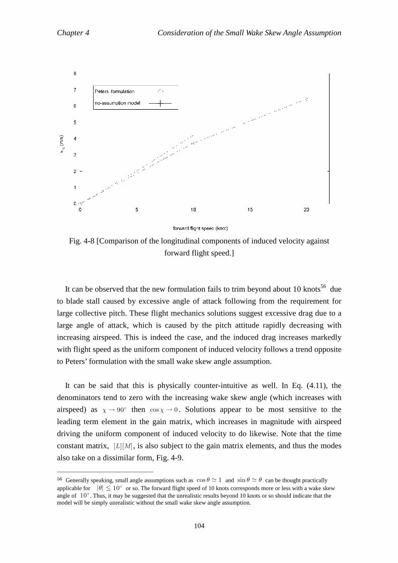
Chapter 4 Consideration of the Small Wake Skew Angle Assumption
104
Fig. 4-8 [Comparison of the longitudinal components of induced velocity against
forward flight speed.]
It can be observed that the new formulation fails to trim beyond about 10 knots56 due
to blade stall caused by excessive angle of attack following from the requirement for
large collective pitch. These flight mechanics solutions suggest excessive drag due to a
large angle of attack, which is caused by the pitch attitude rapidly decreasing with
increasing airspeed. This is indeed the case, and the induced drag increases markedly
with flight speed as the uniform component of induced velocity follows a trend opposite
to Peters’ formulation with the small wake skew angle assumption.
It can be said that this is physically counter-intuitive as well. In Eq. (4.11), the
denominators tend to zero with the increasing wake skew angle (which increases with
airspeed) as 1→ 90 then cos1→ 0 . Solutions appear to be most sensitive to the
leading term element in the gain matrix, which increases in magnitude with airspeed
driving the uniform component of induced velocity to do likewise. Note that the time
constant matrix, [L][M] , is also subject to the gain matrix elements, and thus the modes
also take on a dissimilar form, Fig. 4-9.
56 Generally speaking, small angle assumptions such as cos > ≃ 1 and sin > ≃ > can be thought practically applicable for |>| 10 or so. The forward flight speed of 10 knots corresponds more or less with a wake skew angle of 10 . Thus, it may be suggested that the unrealistic results beyond 10 knots or so should indicate that the model will be simply unrealistic without the small wake skew angle assumption.
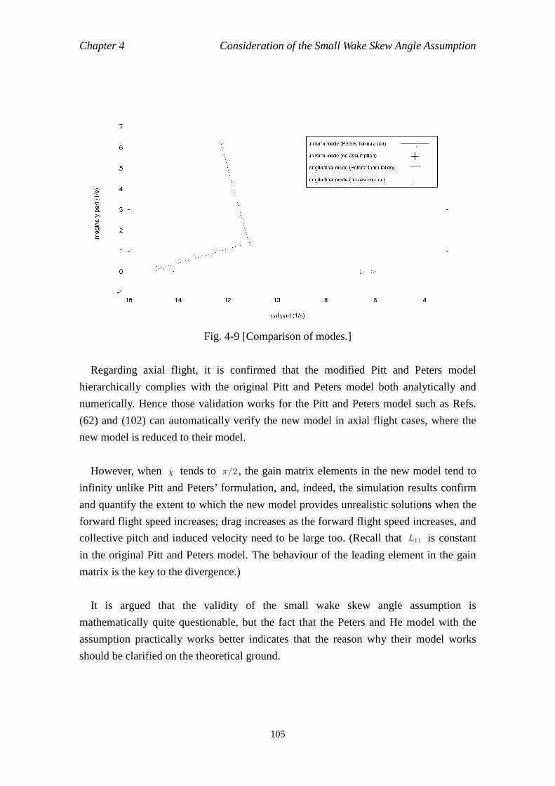
Chapter 4 Consideration of the Small Wake Skew Angle Assumption
105
Fig. 4-9 [Comparison of modes.]
Regarding axial flight, it is confirmed that the modified Pitt and Peters model
hierarchically complies with the original Pitt and Peters model both analytically and
numerically. Hence those validation works for the Pitt and Peters model such as Refs.
(62) and (102) can automatically verify the new model in axial flight cases, where the
new model is reduced to their model.
However, when 1 tends to 2/2 , the gain matrix elements in the new model tend to
infinity unlike Pitt and Peters’ formulation, and, indeed, the simulation results confirm
and quantify the extent to which the new model provides unrealistic solutions when the
forward flight speed increases; drag increases as the forward flight speed increases, and
collective pitch and induced velocity need to be large too. (Recall that L11 is constant
in the original Pitt and Peters model. The behaviour of the leading element in the gain
matrix is the key to the divergence.)
It is argued that the validity of the small wake skew angle assumption is
mathematically quite questionable, but the fact that the Peters and He model with the
assumption practically works better indicates that the reason why their model works
should be clarified on the theoretical ground.
Chapter 4 Consideration of the Small Wake Skew Angle Assumption
106
4.3 Further Discussion 4.3.1 Deductive and Inductive Approaches
The simulation results indicate that the new formulation without the small wake skew
assumption is unrepresentative despite the fact that the derivation must mathematically
be more consistent than that of the Peters and He model. Considering the facts that the
Peters and He model was numerically validated in Refs. (7), (92) and (112) showing
excellent correlation with experimental data and also that its advanced models such as
Refs. (131), (132) and (135) are widely used today, the practical validity of the Peters
and He model can be considered to be fully validated in spite of the questionable
assumption57.
Questions naturally arising from this situation should include an argument if it is
possible to prove why the Peters and He model is practically valid in spite of the
mathematically questionable application of the small wake skew angle assumption. In
order to respond to this question, the possibility to deductively present a proof shall be
first discussed. (A deductive approach can generally provide a logically rigorous proof.)
Generally mathematically speaking, an approximated equation based on an
assumption can approximate the original equation only when the underlying assumption
is valid; hence when the assumption breaks down, the original and the approximated
equations should formally be regarded as different equations. (For example, it is plainly
evident that tan1 and 2 tan(1/2) are different functions, though tan1 can be well
approximated by 2 tan(1/2) when 1 is sufficiently small. They would behave quite
differently when 1 is fairly large.)
It can be thus believed that an attempt to apply the Peters and He model, which is
derived on the small wake skew angle assumption, for larger angles, for which the
assumption breaks down, is mathematically inappropriate or even meaningless in itself,
regardless how the results are experimentally validated. Since the mathematical
consistency in the derivation breaks down when the model is extended to larger wake
skew angles, it is impossible to mathematically discuss the resultant model any further.
There seems to be no mathematically cogent reason available which makes it possible 57 This author informally enquired after the mathematical validity of the assumption to Dr. ChengJian He by email, but his reply reads only that the model was numerically validated in correlation with experimental data. The present author believes that such a numerical validation is weak as a theoretical proof for the validity of the assumption, but any further replies were given. Thus, it still remains unclear how the original authors consider the validity of the assumption purely from the analytical point of view.

Chapter 4 Consideration of the Small Wake Skew Angle Assumption
107
to extend the approximated equations up to those cases in which the approximations are
not valid any longer. Therefore, it can be said that the inappropriateness of the
application of the resultant model for larger wake skew angles is mathematically
evident.
Another mathematically inconsistent point in the derivation is the way of applying
the small wake skew angle assumption. If 1 is really small, then Eqs. (2.67.1) and
(2.67.3) could be further approximated as
x = $ sin1+ x0 ,
≃ $1+ x0 (4.12)
z = $ cos 1.
≃ $ (4.13)
Equations. (2.83.2) - (2.83.3) could also be further approximated as
sin1 ≃ 1, (4.14)
tan1 ≃ 1. (4.15)
The reasons why the small wake skew angle assumption is not applied before Eq.
(2.85) in the derivation or why Eqs. (2.83.2) and (2.83.3) are not approximated down to
1 are not explained in Ref. (7) at all. The way of applying the assumption in the
original derivation is thus considered mathematically inconsistent.
Since logical debâcles with regard to the above-mentioned points are evident, the gap
between the questionable derivation and the experimental validity of the resultant model
cannot be filled by a deductive discussion within the present frame of the derivation.
This may indicate that the only possibility to deductively justify the assumption, if
any, may lie in a fundamental extension of the model derivation by introducing new
(more reasonable) assumptions, which shall be related to those physical phenomena that
are hugely simplified or not considered at all in the original model, to construct
consistent logics. Indeed, there are quite a few ignored or oversimplified physical
phenomena in the original derivation. (For example, the cylindrical description of the
wake tube itself is a crudest modelling of a wake tube and thus quite unrealistic.) When
extending the original model derivation by taking new physical aspects into
Chapter 4 Consideration of the Small Wake Skew Angle Assumption
108
consideration, there are generally two possible approaches; (i) building a completely
new model from scratch with the aim to outperform the Peters and He model with a
more mathematically consistent derivation, and (ii) modifying the present derivation of
Peters and He model with the aim to have the same resultant model with a more
mathematically consistent derivation.
With regard to the former approach, if the new model outperforms or works at least
as well as the Peters and He model, then the paradox with the small wake skew angle
assumption may be considered to be ascribed to the newly incorporated physical aspects.
However, even if the new model performs well, the new model should also require
experimental validation, and thus this cannot be a conclusive mathematical proof
against the small wake skew angle assumption. (Recall that the Peters and He model is
already experimentally validated implying that the small wake skew angle assumption
is practically useful. As long as the extension of the present model should (even partly)
rely on an experimental method, it is logically difficult to rigorously refute the small
wake skew assumption thereby.) In addition, new assumptions related to the new
physical aspects shall be new problems to experimentally validate because the effects of
these physical phenomena are not easily evaluated theoretically. In any case, a new
model should be considered as a different model from the Peters and He model and thus
cannot be a theoretical counter-proof against the derivation of the Peters and He model.
Also, building a completely new dynamic inflow model together with its validation
should be beyond the scope of this thesis.
With regard to the latter approach, even though it were possible to ascribe the
paradox with the small wake skew angle assumption to some new physical phenomena,
since there should still be many simplifications and neglected physical phenomena in
the original derivation, the selection of those physical phenomena which to newly
introduce should inevitably be purposeful and intentional to some extent, as long as the
derivation is aimed to result in the same representation as that of the Peters and He
model. In order to theoretically verify the selection, it is required to exclude all the other
possibilities which may be related to the wake skew angle; otherwise the selection can
be considered as a purposefully far-fetched. However, this probatio diabolica is
logically impossible to carry out.
Based on the discussion above, this author concludes that a deductive approach
towards the paradox regarding the small wake skew angle assumption is impossible
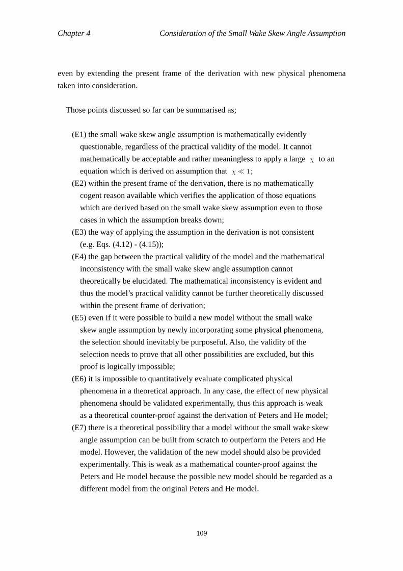
Chapter 4 Consideration of the Small Wake Skew Angle Assumption
109
even by extending the present frame of the derivation with new physical phenomena
taken into consideration.
Those points discussed so far can be summarised as;
(E1) the small wake skew angle assumption is mathematically evidently
questionable, regardless of the practical validity of the model. It cannot
mathematically be acceptable and rather meaningless to apply a large 1 to an
equation which is derived on assumption that 1 1 ;
(E2) within the present frame of the derivation, there is no mathematically
cogent reason available which verifies the application of those equations
which are derived based on the small wake skew assumption even to those
cases in which the assumption breaks down;
(E3) the way of applying the assumption in the derivation is not consistent
(e.g. Eqs. (4.12) - (4.15));
(E4) the gap between the practical validity of the model and the mathematical
inconsistency with the small wake skew angle assumption cannot
theoretically be elucidated. The mathematical inconsistency is evident and
thus the model’s practical validity cannot be further theoretically discussed
within the present frame of derivation;
(E5) even if it were possible to build a new model without the small wake
skew angle assumption by newly incorporating some physical phenomena,
the selection should inevitably be purposeful. Also, the validity of the
selection needs to prove that all other possibilities are excluded, but this
proof is logically impossible;
(E6) it is impossible to quantitatively evaluate complicated physical
phenomena in a theoretical approach. In any case, the effect of new physical
phenomena should be validated experimentally, thus this approach is weak
as a theoretical counter-proof against the derivation of Peters and He model;
(E7) there is a theoretical possibility that a model without the small wake skew
angle assumption can be built from scratch to outperform the Peters and He
model. However, the validation of the new model should also be provided
experimentally. This is weak as a mathematical counter-proof against the
Peters and He model because the possible new model should be regarded as a
different model from the original Peters and He model.
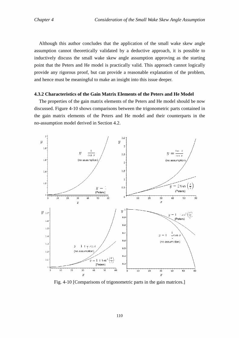
Chapter 4 Consideration of the Small Wake Skew Angle Assumption
110
Although this author concludes that the application of the small wake skew angle
assumption cannot theoretically validated by a deductive approach, it is possible to
inductively discuss the small wake skew angle assumption approving as the starting
point that the Peters and He model is practically valid. This approach cannot logically
provide any rigorous proof, but can provide a reasonable explanation of the problem,
and hence must be meaningful to make an insight into this issue deeper.
4.3.2 Characteristics of the Gain Matrix Elements of the Peters and He Model
The properties of the gain matrix elements of the Peters and He model should be now
discussed. Figure 4-10 shows comparisons between the trigonometric parts contained in
the gain matrix elements of the Peters and He model and their counterparts in the
no-assumption model derived in Section 4.2.
Fig. 4-10 [Comparisons of trigonometric parts in the gain matrices.]
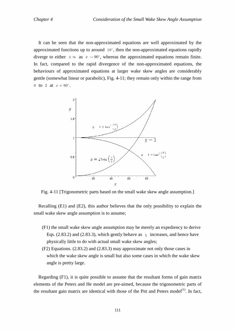
Chapter 4 Consideration of the Small Wake Skew Angle Assumption
111
It can be seen that the non-approximated equations are well approximated by the
approximated functions up to around 10 , then the non-approximated equations rapidly
diverge to either ∞ as x→ 90, whereas the approximated equations remain finite.
In fact, compared to the rapid divergence of the non-approximated equations, the
behaviours of approximated equations at larger wake skew angles are considerably
gentle (somewhat linear or parabolic), Fig. 4-11; they remain only within the range from
0 to 2 at x = 90 .
Fig. 4-11 [Trigonometric parts based on the small wake skew angle assumption.]
Recalling (E1) and (E2), this author believes that the only possibility to explain the
small wake skew angle assumption is to assume;
(F1) the small wake skew angle assumption may be merely an expediency to derive
Eqs. (2.83.2) and (2.83.3), which gently behave as 1 increases, and hence have
physically little to do with actual small wake skew angles;
(F2) Equations. (2.83.2) and (2.83.3) may approximate not only those cases in
which the wake skew angle is small but also some cases in which the wake skew
angle is pretty large.
Regarding (F1), it is quite possible to assume that the resultant forms of gain matrix
elements of the Peters and He model are pre-aimed, because the trigonometric parts of
the resultant gain matrix are identical with those of the Pitt and Peters model(1). In fact,
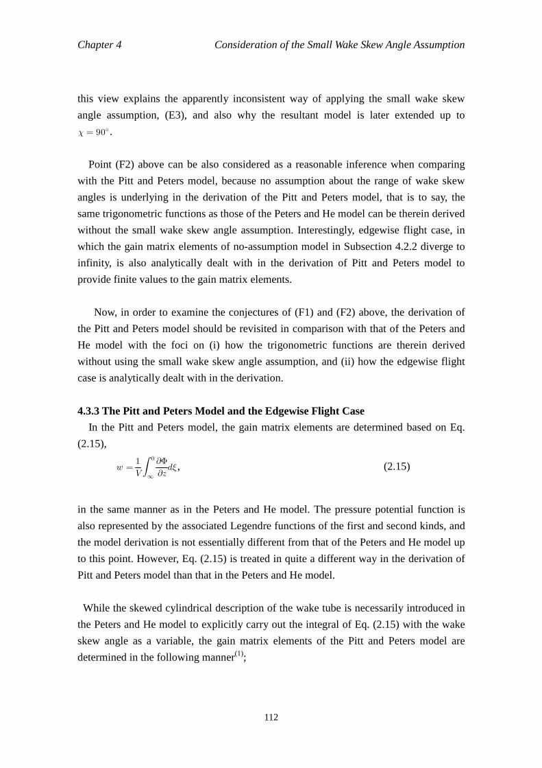
Chapter 4 Consideration of the Small Wake Skew Angle Assumption
112
this view explains the apparently inconsistent way of applying the small wake skew
angle assumption, (E3), and also why the resultant model is later extended up to
1 = 90 .
Point (F2) above can be also considered as a reasonable inference when comparing
with the Pitt and Peters model, because no assumption about the range of wake skew
angles is underlying in the derivation of the Pitt and Peters model, that is to say, the
same trigonometric functions as those of the Peters and He model can be therein derived
without the small wake skew angle assumption. Interestingly, edgewise flight case, in
which the gain matrix elements of no-assumption model in Subsection 4.2.2 diverge to
infinity, is also analytically dealt with in the derivation of Pitt and Peters model to
provide finite values to the gain matrix elements.
Now, in order to examine the conjectures of (F1) and (F2) above, the derivation of
the Pitt and Peters model should be revisited in comparison with that of the Peters and
He model with the foci on (i) how the trigonometric functions are therein derived
without using the small wake skew angle assumption, and (ii) how the edgewise flight
case is analytically dealt with in the derivation.
4.3.3 The Pitt and Peters Model and the Edgewise Flight Case
In the Pitt and Peters model, the gain matrix elements are determined based on Eq.
(2.15),
w =V
1∫
∞
0
∂z
∂Φd$ , (2.15)
in the same manner as in the Peters and He model. The pressure potential function is
also represented by the associated Legendre functions of the first and second kinds, and
the model derivation is not essentially different from that of the Peters and He model up
to this point. However, Eq. (2.15) is treated in quite a different way in the derivation of
Pitt and Peters model than that in the Peters and He model.
While the skewed cylindrical description of the wake tube is necessarily introduced in
the Peters and He model to explicitly carry out the integral of Eq. (2.15) with the wake
skew angle as a variable, the gain matrix elements of the Pitt and Peters model are
determined in the following manner(1);
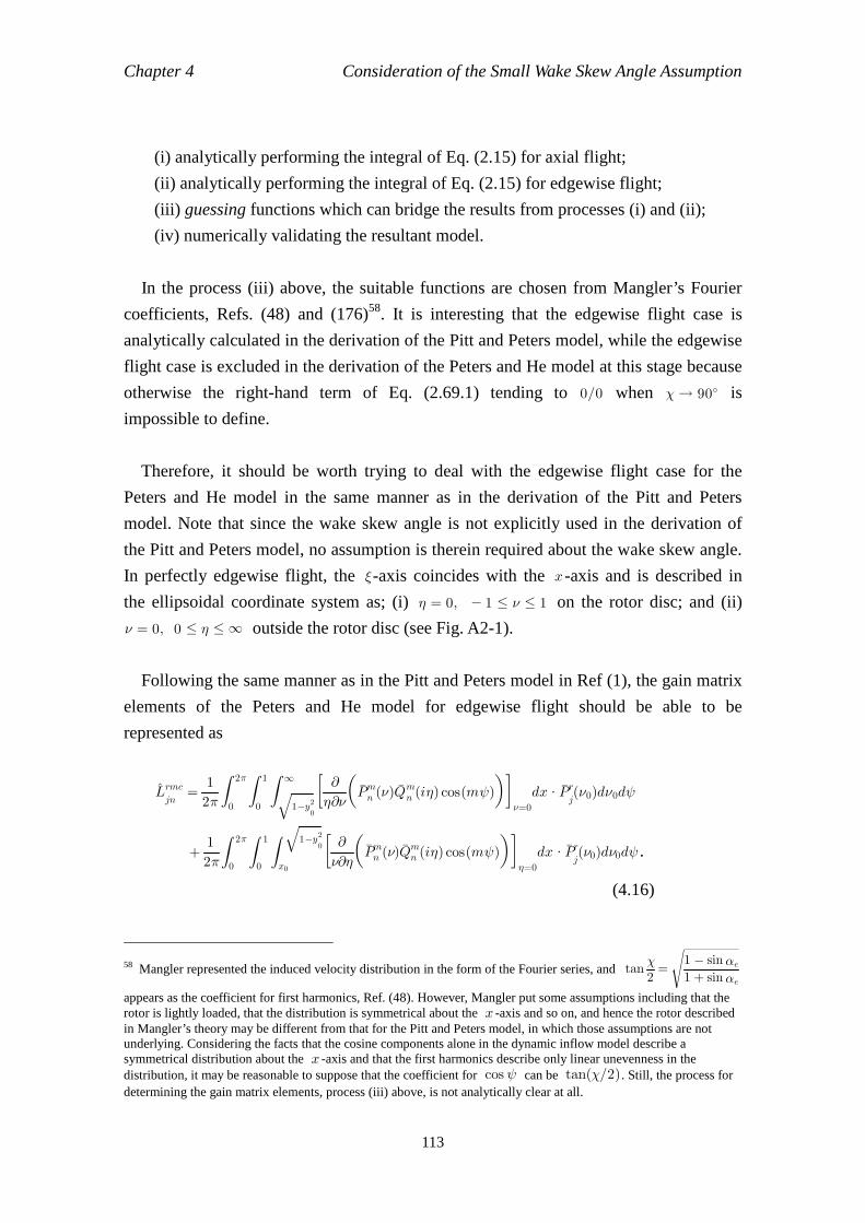
Chapter 4 Consideration of the Small Wake Skew Angle Assumption
113
(i) analytically performing the integral of Eq. (2.15) for axial flight;
(ii) analytically performing the integral of Eq. (2.15) for edgewise flight;
(iii) guessing functions which can bridge the results from processes (i) and (ii);
(iv) numerically validating the resultant model.
In the process (iii) above, the suitable functions are chosen from Mangler’s Fourier
coefficients, Refs. (48) and (176)58. It is interesting that the edgewise flight case is
analytically calculated in the derivation of the Pitt and Peters model, while the edgewise
flight case is excluded in the derivation of the Peters and He model at this stage because
otherwise the right-hand term of Eq. (2.69.1) tending to 0/0 when 1→ 90 is
impossible to define.
Therefore, it should be worth trying to deal with the edgewise flight case for the
Peters and He model in the same manner as in the derivation of the Pitt and Peters
model. Note that since the wake skew angle is not explicitly used in the derivation of
the Pitt and Peters model, no assumption is therein required about the wake skew angle.
In perfectly edgewise flight, the $-axis coincides with the x -axis and is described in
the ellipsoidal coordinate system as; (i) & = 0, 1 1 on the rotor disc; and (ii)
= 0, 0 & ∞ outside the rotor disc (see Fig. A2-1).
Following the same manner as in the Pitt and Peters model in Ref (1), the gain matrix
elements of the Peters and He model for edgewise flight should be able to be
represented as
L rmcjn
=22
1∫
0
22∫
0
1∫
1y20
√
∞
&∂
∂
Pmn ()Qmn (i&) cos(mψ)
=0
dx Prj(0)d0dψ
+22
1∫
0
22∫
0
1∫
x0
1y20
√
∂&
∂
Pmn ()Qmn (i&) cos(mψ)
&=0
dx Prj(0)d0dψ .
(4.16)
58 Mangler represented the induced velocity distribution in the form of the Fourier series, and tan2
1=
1 + sin:e
1 sin:e√
appears as the coefficient for first harmonics, Ref. (48). However, Mangler put some assumptions including that the rotor is lightly loaded, that the distribution is symmetrical about the x -axis and so on, and hence the rotor described in Mangler’s theory may be different from that for the Pitt and Peters model, in which those assumptions are not underlying. Considering the facts that the cosine components alone in the dynamic inflow model describe a symmetrical distribution about the x -axis and that the first harmonics describe only linear unevenness in the distribution, it may be reasonable to suppose that the coefficient for cos ψ can be tan(1/2). Still, the process for determining the gain matrix elements, process (iii) above, is not analytically clear at all.
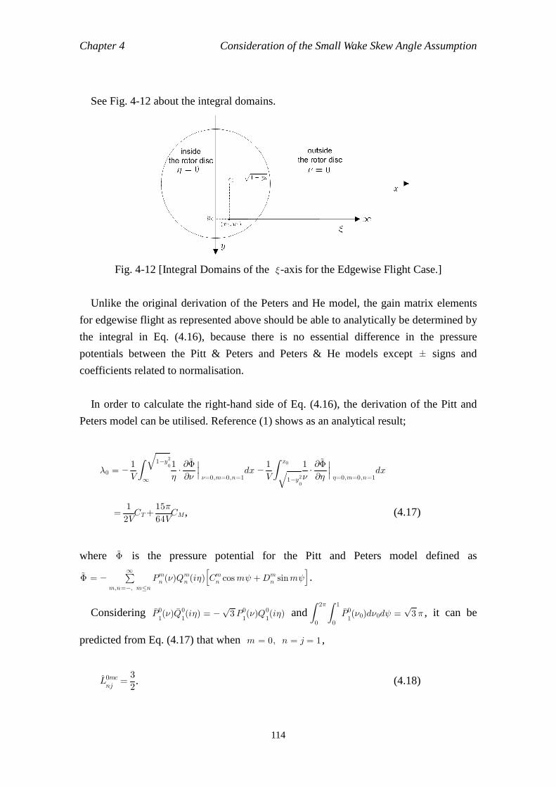
Chapter 4 Consideration of the Small Wake Skew Angle Assumption
114
See Fig. 4-12 about the integral domains.
Fig. 4-12 [Integral Domains of the $-axis for the Edgewise Flight Case.]
Unlike the original derivation of the Peters and He model, the gain matrix elements
for edgewise flight as represented above should be able to analytically be determined by
the integral in Eq. (4.16), because there is no essential difference in the pressure
potentials between the Pitt & Peters and Peters & He models except signs and
coefficients related to normalisation.
In order to calculate the right-hand side of Eq. (4.16), the derivation of the Pitt and
Peters model can be utilised. Reference (1) shows as an analytical result;
?0 = V
1∫
∞
1y20
√
&
1 ∂
∂Φ!=0,m=0,n=1
dx V
1∫
1y20
√
x0
1 ∂&
∂Φ!&=0,m=0,n=1
dx
=2V
1CT+
64V
152CM, (4.17)
where Φ! is the pressure potential for the Pitt and Peters model defined as
Φ! = ∑
m,n=, mn
∞Pmn ()Q
mn (i&)
[
Cmn cosmψ +Dmn sinmψ
]
.
Considering P01()Q 0
1(i&) = 3
√P01()Q0
1(i&) and
∫
0
22∫
0
1
P01(0)d0dψ = 3
√2 , it can be
predicted from Eq. (4.17) that when m = 0, n = j = 1 ,
L0mcnj
=2
3. (4.18)
Chapter 4 Consideration of the Small Wake Skew Angle Assumption
115
This result coincides with Eq. (2.102.1), which is derived on the small wake skew
angle assumption. This coincidence is highly interesting when recalling the
no-assumption model in Section 4.2, whose gain matrix elements diverge to infinity at
1 = 90 .
In the derivation of the Pitt and Peters model, other gain matrix elements such as
L13, L31 and L33 are also analytically obtained. (Note that it is stated in Ref. (1) that
L22 is an exception, and only a numerical result of L22 ≃ 2 is therein shown.) Since
there is no essential difference in the pressure potentials between the Pitt & Peters and
Peters & He models except coefficients it can be considered that Eq. (4.16) is possible
to analytically calculate also for other combinations of m , n, r and j for edgewise
flight. The coincidence between Eqs. (4.18) and (2.102.1) should strengthen views (F1)
and (F2) above that the small wake skew angle assumption has little to do with actual
wake skew angles; the assumption rather seems to be playing a role in bridging axial
and edgewise flights.
Since both Eq. (4.18) and the no-assumption model, in which L00c11 → ∞ for edgewise
flight, are analytically derived, there must be another analytical difference which made
their results so different in their derivations. When comparing Eq. (4.16) and Eq. (2.65),
it can be noticed that while Eq. (4.16) have two terms related to ∂/∂ and ∂/∂& ,
respectively, Eq. (2.65) has only one term related to ∂/∂& . At the stage when Eq. (2.65)
is derived, the small wake skew angle assumption is not yet applied, and hence it can be
believed that the difference is brought independently of the small wake skew angle
assumption. Indeed, the ∂/∂ term is missed out from the derivation of the Peters and
He model when Eq. (2.49) is simplified to Eq. (2.50)59. This simplification should be
fully justified for the derivation of the apparent mass matrix elements because the
derivation is based on Eq. (2.17) without any integrals. However, the simplification is
maybe not appropriate for the derivation of the gain matrix elements because the
integral path along the $-axis is not restricted only in the domain which is described as
& = 0 . Thus, even for obtaining the induced velocity distribution on the rotor disc, it is
considered that & = 0 should be substituted only after the integral along the $-axis is
59 The derivation of the no-assumption model in Section 4.2 is entirely based on that of the Peters and He model, except for the small wake skew angle assumption. The fact that the no-assumption model, which must mathematically be more consistent, breaks down for edgewise flight should indicate that the key to explain the difference between Eq. (4.18) and the divergence to infinity would lie in other part of the original derivation of the Peters and He model than the small wake skew angle assumption itself. This observation is consistent with the identification of the difference between Eqs. (4.19) and (2.65).

Chapter 4 Consideration of the Small Wake Skew Angle Assumption
116
completed.
Based on this view, Eq. (2.65.1) can be extended by using Eq. (2.49) as
L rmcjn
= 22
1∫
0
22∫
0
1∫
0
∞[
2 + &2&(1 2)
∂
∂
Pmn ()Qmn (i&) cos(mψ)
)
+2 + &2(1 + &2)
∂&
∂
Pmn ()Qmn (i&) cos(mψ)
]
d$
&=0
Prj(0) cos(rψ)ddψ .
(4.19)
Now, the possibility of further pressing on the integral of Eq. (4.19) analytically shall
be examined. The $-axis is represented in the ellipsoidal coordinates as
$ = 2 20 2 + &2 2y2
0 2 [(1 + &2)(1 2) y2
0](1 y2
0 2
0)
√√
,
(4.20)
and thus
d$ =J 2 2 + &2 2
0 2y2
0 2J
√
J (1 + &2)(1 y20 2
0)d
J 2 2 + &2 20 2y2
0 2J
√
&J &(1 2)(1 y20 2
0)d& ,
(4.21)
where J = [(1 + &2)(1 2) y20](1 y2
0 2
0)
√
.
Also, along the $-axis, and & satisfy
1 + &2 2 &22 y20
√
1 y20 2
0
√
= t& , (4.22)
where
t tan1 = &
(1 + &2)(1 2) y20
√
1 y20 2
0
√
. (4.23)
Therefore, along the $-axis,
Chapter 4 Consideration of the Small Wake Skew Angle Assumption
117
d = &(1 + &2 y2
0 (1 2 + &2 &22 y2
0)(1 y2
0 2
0)
√
)
(1 2 y20 (1 2 + &2 &22 y2
0)(1 y2
0 2
0)
√
)d& . (4.24)
Also, from Eq. (4.22), can be represented as a function of & along the $-axis,
=cos2 1+ &2
& 1 y20 2
0
√
sin1+ K√
cos 1, (for > 0) (4.25)
where
K = &2(&2 + 1) + 20(&2 + 1)cos2 1 &2y2
0sin2 1. (4.26)
Inserting Eqs. (4.21), (4.24), (4.25) and (4.26) into Eq. (4.19) gives an integral of &
alone with the integral domain of & from 0 to ∞.
It can be easily confirmed that when m = r = 0 , n = j = 1 , 0 = 1 , 1 = 0 , y0 = 0 ,
∫
0
∞
∂z
∂Φd$ =
∫
∞
0
3√
tan1
&
1
1 + &23
√&)
d& = 3√
. (4.27)
Thus, for this special case, Eq. (4.19) will be
L 00c11=22
3∫
0
22∫
0
1
d0dψ =2
3 . (4.28)
The coincidence between Eqs. (4.28) and (2.102.1) indicates that Eq. (4.19)
hierarchically covers the axial flight case of the Peters and He model. Also, it can be
shown that Eq. (4.19) naturally accommodate Eq. (4.16), which is derived from Eq.
(4.19) by assuming two extreme cases, = 0 and & = 0 , respectively. Therefore, it can
be said that Eq. (4.19) should describe more general cases varying from axial to
edgewise flights. Equation (4.19) can also naturally reduce down to Eq. (2.50) when
& = 0 for the derivation of the apparent mass matrix.
It should be hoped that an analytical solution could be provided from Eq. (4.19) for
an arbitrary combination of 0 , y0 , m , n, r, j and 1. However, it is turned out to be
Chapter 4 Consideration of the Small Wake Skew Angle Assumption
118
extremely difficult to analytically carry out the integrals appearing in Eq. (4.19) even
for some simple cases such as m = r = 1 and n = j = 2 . Since the primary aim of this
Chapter is not providing a new model but clarifying the paradox with the small wake
skew angle assumption, an attempt to analytically complete the integrals in Eq. (4.19)
for a general case can be abandoned now. Instead, the two terms in the right-hand side
of Eq. (4.19) shall be qualitatively discussed below.
When equals 1 (i.e. axial flight for a streamline running through the hub centre),
&(1 2)/(2 + &2) becomes zero and thus only the second term remains. As long as the
wake skew angle is sufficiently small, is nearly zero over the most part of the
streamline, and hence the contribution of the first term can still be considered small. On
the other hand, (1 + &2)/(2 + &2) becomes nearly 1 when is close to 1 . Also,
& → ∞ as $ → ∞ , and thus (1 + &2)/(2 + &2) → 1 as $ → ∞ regardless of 0 or
1 ( =2/2), thus the contribution of the second term cannot generally be ignored. This is
indeed the case with the formulation of the Peters and He model, in which the first term
is ignored but the wake skew angle is assumed to be small. Thus, the derivation of
Peters and He model and the small wake skew angle assumption can be considered
consistent in this case.
In perfectly edgewise flight (when exactly 1 = 2/2), the $-axis coincides with the
x -axis and becomes constantly zero outside the rotor disc, and thus the second term
of Eq. (4.19) is scored out in the domain. In this case, it is believed that the first term is
playing a crucial role. The huge difference between the no-assumption model, in which
L00c11 → ∞ as 1 → 2/2 , and Eq. (4.28) is thus likely ascribed to the fact that the first term
is ignored in the derivation of the Peters and He model.
It should be difficult to make a general comment for an arbitrary combination of
m, n, r, j and 1, but based on the discussion above, what can be therefrom predicted
include that (i) if the wake skew angle is sufficiently small, the contribution of the first
term of Eq. (4.19) should be negligible regardless of 0 , and (ii) if the wake skew angle
is close to 2/2 , the first term of Eq. (4.19) may largely affect the results.
Point (i) above is consistent with the formulation of the Peters and He model
including the small wake skew angle assumption, and point (ii) is underpinned when
considering the difference between the edgewise cases between Eqs. (4.18) and the
no-assumption model in Section 4.2, because edgewise flight and other flight scenarios
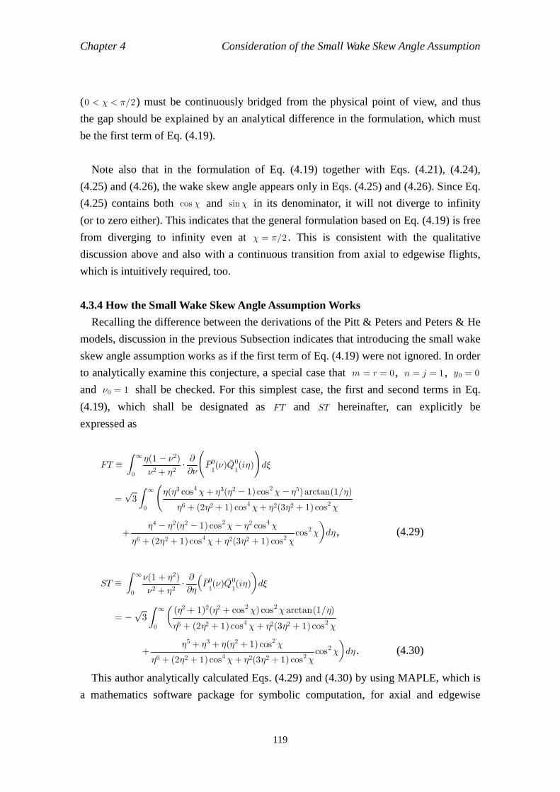
Chapter 4 Consideration of the Small Wake Skew Angle Assumption
119
(0 < 1 < 2/2) must be continuously bridged from the physical point of view, and thus
the gap should be explained by an analytical difference in the formulation, which must
be the first term of Eq. (4.19).
Note also that in the formulation of Eq. (4.19) together with Eqs. (4.21), (4.24),
(4.25) and (4.26), the wake skew angle appears only in Eqs. (4.25) and (4.26). Since Eq.
(4.25) contains both cos 1 and sin1 in its denominator, it will not diverge to infinity
(or to zero either). This indicates that the general formulation based on Eq. (4.19) is free
from diverging to infinity even at 1 = 2/2 . This is consistent with the qualitative
discussion above and also with a continuous transition from axial to edgewise flights,
which is intuitively required, too.
4.3.4 How the Small Wake Skew Angle Assumption Works
Recalling the difference between the derivations of the Pitt & Peters and Peters & He
models, discussion in the previous Subsection indicates that introducing the small wake
skew angle assumption works as if the first term of Eq. (4.19) were not ignored. In order
to analytically examine this conjecture, a special case that m = r = 0 , n = j = 1 , y0 = 0
and 0 = 1 shall be checked. For this simplest case, the first and second terms in Eq.
(4.19), which shall be designated as FT and ST hereinafter, can explicitly be
expressed as
FT ∫
0
∞
2 + &2&(1 2)
∂
∂
P01()Q 0
1(i&)
)
d$
= 3√ ∫
0
∞
&6 + (2&2 + 1) cos4 1+ &2(3&2 + 1)cos21
&(&3 cos4 1+ &3(&2 1) cos21 &5) arctan(1/&)
+&6 + (2&2 + 1) cos4 1+ &2(3&2 + 1) cos2 1
&4 &2(&2 1) cos2 1 &2 cos4 1cos2 1
d& , (4.29)
ST ∫
0
∞
2 + &2(1 + &2)
∂&
∂
P01()Q 0
1(i&)
d$
= 3√ ∫
0
∞
&6 + (2&2 + 1) cos4 1+ &2(3&2 + 1)cos2 1
(&2 + 1)2(&2 + cos2 1) cos21arctan(1/&)
+&6 + (2&2 + 1) cos4 1+ &2(3&2 + 1) cos2 1
&5 + &3 + &(&2 + 1) cos2 1cos2 1
d& . (4.30)
This author analytically calculated Eqs. (4.29) and (4.30) by using MAPLE, which is
a mathematics software package for symbolic computation, for axial and edgewise
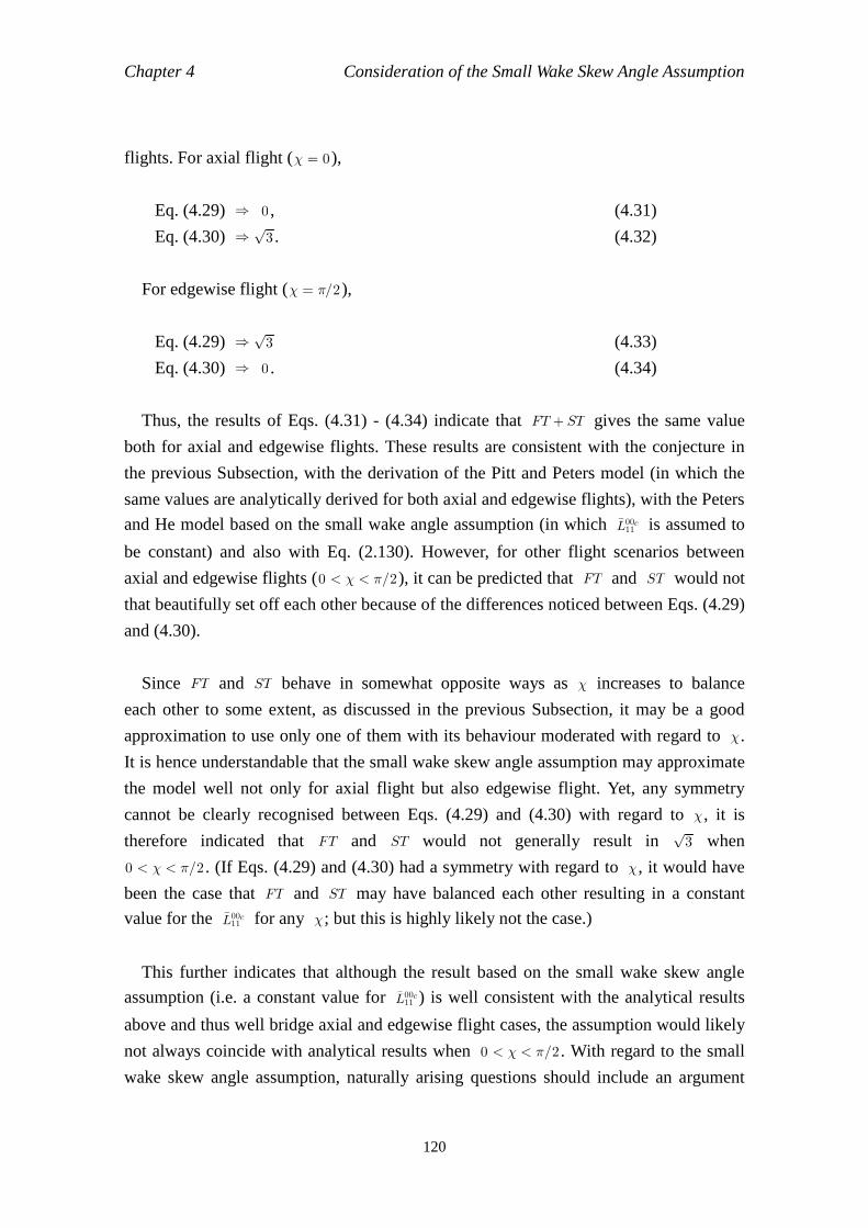
Chapter 4 Consideration of the Small Wake Skew Angle Assumption
120
flights. For axial flight (1 = 0),
Eq. (4.29) ⇒ 0 , (4.31)
Eq. (4.30) ⇒ 3√
. (4.32)
For edgewise flight (1 = 2/2),
Eq. (4.29) ⇒ 3√
(4.33)
Eq. (4.30) ⇒ 0 . (4.34)
Thus, the results of Eqs. (4.31) - (4.34) indicate that FT + ST gives the same value
both for axial and edgewise flights. These results are consistent with the conjecture in
the previous Subsection, with the derivation of the Pitt and Peters model (in which the
same values are analytically derived for both axial and edgewise flights), with the Peters
and He model based on the small wake angle assumption (in which L00c11 is assumed to
be constant) and also with Eq. (2.130). However, for other flight scenarios between
axial and edgewise flights (0 < 1 < 2/2), it can be predicted that FT and ST would not
that beautifully set off each other because of the differences noticed between Eqs. (4.29)
and (4.30).
Since FT and ST behave in somewhat opposite ways as 1 increases to balance
each other to some extent, as discussed in the previous Subsection, it may be a good
approximation to use only one of them with its behaviour moderated with regard to 1.
It is hence understandable that the small wake skew angle assumption may approximate
the model well not only for axial flight but also edgewise flight. Yet, any symmetry
cannot be clearly recognised between Eqs. (4.29) and (4.30) with regard to 1, it is
therefore indicated that FT and ST would not generally result in 3√
when
0 < 1 < 2/2 . (If Eqs. (4.29) and (4.30) had a symmetry with regard to 1, it would have
been the case that FT and ST may have balanced each other resulting in a constant
value for the L00c11 for any 1; but this is highly likely not the case.)
This further indicates that although the result based on the small wake skew angle
assumption (i.e. a constant value for L00c11 ) is well consistent with the analytical results
above and thus well bridge axial and edgewise flight cases, the assumption would likely
not always coincide with analytical results when 0 < 1 < 2/2 . With regard to the small
wake skew angle assumption, naturally arising questions should include an argument
Chapter 4 Consideration of the Small Wake Skew Angle Assumption
121
whether the assumption provides analytical solutions for some reason or it provides
mere approximations. In point of fact, the sheer coincidence of the trigonometric
functions in the gain matrix of the Peters and He model with those of the Pitt and Peters
model would naturally make readers face a question if there is a hidden mathematical
reason which allows the questionable application of the assumption to provide
analytical solutions.
This author discussed only a special case of L00c11 , but believes that the discussion
above should suffice as a counter-proof in response to the question above to show that
the small wake skew angle assumption does not provide analytically rigorous results for
all 1 ∈ [0, 2/2] . Moreover, the present author adds following two reasons to conclude
that the small wake skew angle assumption does not provide analytical solutions; (i) the
way of applying the assumption in the original derivation is analytically not consistent,
E(3), and; (ii) in the derivation of the Pitt and Peters model, it is stated that L22 for
edgewise flight cannot analytically derived unlike other gain matrix elements, and it is
only numerically shown that L22 ≃ 2 . This indicates that L11s22 = 2 for 1 = 2/2 in the
Peters and He model is not consistent with its fully analytical result60. This conclusion
should be consistent with points (E1), (E2) and (E3), and also with conjectures (F1) and
(F2).
In any case, in order to more generally and rigorously discuss if ST together with the
small wake skew angle assumption can well approximate those results which are
derived from FT and ST for axial and edgewise flight cases, Eq. (4.19) ideally needs
to be analytically calculated to a closed-form as a function of 1. However, it is turned
out that it is extremely difficult to press on the integrals for more general cases. This
potentially intensive calculation must be well beyond the scope of this thesis, and hence
this author believes that this problem can be left as a good future problem.
It is believed that this problem needs to be concluded through more concrete proofs
and discussion. Especially, it is necessary that the original authors would join the
discussion to provide clear and coherent explanations about (i) the difference between
the Pitt & Peters and Peters & He models in the treatments of the edgewise flight cases,
and (ii) how the small wake skew angle assumption can be analytically validated. It is
60 Indeed, there is a certain symmetry recognised between the two terms in Eq. (4.19) with regard to and & . For example, Eq. (4.19) approximately reduces to (1/)(∂Φ/∂&) and (1/&)(∂Φ/∂) for axial and edgewise flights, respectively. However, the present author was not able enough to draw a conclusion to the problem if there is any logical connection between this symmetry and the practical validity of the small wake skew angle assumption.
Chapter 4 Consideration of the Small Wake Skew Angle Assumption
122
hoped that this thesis would provoke further discussion of this problem.
4.4 Chapter Summary This is arguably the first study which identified the paradoxical aspects of the small
wake skew angle assumption in the derivation of Peters and He model. A new model
based on the derivation of Peters and He model was proposed without the assumption,
but this model does not work well. This further led to the discussion why the Peters and
He model practically works so well in spite of the questionable assumption. In so doing,
the difference between the Pitt & Peters and Peters & He models in the treatments of the
edgewise flight cases was identified and the paradox with the small wake skew angle
was explained in relation to the difference.
Discussed points and results in this Chapter can be summarised as follows:
1. Regarding the small wake skew angle assumption used in the derivation of the
Peters and He model, this author points out its mathematical inconsistency and
inappropriateness. A new model is proposed without using the assumption, but the
results suggested by the model are counter to reality;
2. This author discussed why the Peters and He model practically works well in spite
of the questionable application of the small wake skew angle assumption in the
derivation. In so doing, the possibility of deductively proving the validity of the
assumption is ruled out, and thus only inductive discussions are made on the
assumption that the Peters and He model is practically valid;
3. Due to the mathematical inconsistency that the resultant model is extended to large
wake skew angles, this author conjectured that the small wake skew angle
assumption has little to do with an actual wake skew angle, but may play a role in
approximating the model for some specific flight cases including a flight case with
a large wake skew angle such as edgewise flight;
4. Since the gain matrix elements in the Pitt and Peters model for edgewise flight are
analytically determined, this author applied the same approach for the gain matrix
elements of the Peters and He model without using the small wake skew angle
assumption, and obtained the same result as those of the original model, which is
derived based on the assumption;
5. By comparing the equation for edgewise flight in the derivation of Pitt and Peters
model and the Peters and He model, this author points out that the base equation of
the Peters and He model, Eq. (2.50), lacks one term related to ∂/∂ . It is identified
Chapter 4 Consideration of the Small Wake Skew Angle Assumption
123
that the pertinent term is left out when Eq. (2.49) is simplified to Eq. (2.50), but the
simplification is maybe not appropriate for generally deriving the gain matrix
elements;
6. The properties of two terms contained in Eq. (2.49) are qualitatively discussed. It is
confirmed that the first term, which is left out at the simplification, may not hugely
affect the result when the wake skew angle is nearly zero. Thus, the derivation of
the Peters and He model, in which the first term is ignored but the wake skew angle
is assumed to be small, is consistent in this point;
7. It is qualitatively discussed that the two terms contained in Eq. (2.49) behave
somewhat in opposite ways as the wake skew angle increases. Thus, it can be
considered reasonable to think that only the second term in Eq. (2.49) together with
the small wake skew angle assumption may approximate the equation both for axial
and edgewise flights to some extent;
8. Since it is turned out that analytically carrying out the integrals in Eq. (4.19) should
be extremely difficult, only the simplest special case with L00c11 is examined to test
the prediction above. It is confirmed that the axial and edgewise flight cases result
in the same value, as if the small wake skew angle assumption were therein
assumed, due to the opposite tendencies that the two terms in Eq. (4.19) have. Still,
the two terms do not have a perfect symmetry with regard to the wake skew angle.
This likely indicate that they would not always balance out for 0 < 1 < 2/2 ;
9. It can be predicted that the small wake skew angle assumption may more generally
approximate the axial and edgewise flight cases. However, in order to confirm this
conjecture more rigorously, it is to be hoped in the future that the integrals in Eq.
(4.19) will be fully analytically completed to a closed-form as a function of 1.
Chapter 5 Conclusions and Future Directions
124
Chapter 5
Conclusions and Future Directions
5.1 Introductory Remarks - Review of the Research Aim and Objectives
The predefined aim of this research project is to theoretically build a dynamic inflow
model that is suitable for autorotative rotors. The dynamic inflow model for the
helicopter has been intensively developed by Peters and his co-workers over the last two
decades, but little theoretical attention has hitherto been paid to the possible application
of the model to the autorotative rotors, which include rotors of gyroplanes and
autorotating helicopters.
The literature suggests that this should be the first time that the dynamic inflow
model has been theoretically examined for autorotative rotors, and it is hoped that this
thesis will offer a valuable contribution to control analyses of gyroplanes and
helicopters in autorotation. Since this thesis sought to develop a new application of the
dynamic inflow mode, the theory of the dynamic inflow model needed to be thoroughly
re-examined in order to identify the necessary modification. Consequently, the research
objectives were defined as the following three steps:
(i) to critically review the theoretical derivation of the contemporary dynamic inflow
models in detail;
(ii) to examine whether these contemporary dynamic inflow models can also be applied
to autorotative rotors;
(iii) to identify necessary modifications to the contemporary dynamic inflow model in
order that this model can be applied to autorotative rotors.
Clearly a desired outcome of this investigation would have been the determination
that existing dynamic inflow models can be applied to autorotative rotors without
modification. In such a scenario step (iii) above would be unnecessary, while steps (i)
and (ii) would still have been required establishing a theoretical verification of the
modified model.
The next Section summarises these results.
Chapter 5 Conclusions and Future Directions
125
5.2 Conclusions The author first examined in detail the derivation of the Peters and He dynamic
inflow model, which is originally designed for helicopters in the normal working state,
and also considered whether it can be used also for gyroplanes. As a result, the
following results and observations are obtained:
1. The Peters and He model can be used for autorotative rotors without any change in
the matrix elements, but a modification is necessary in the mass-flow parameter.
2. Other dynamic inflow models such as the Pitt and Peters model also follow
Conclusion 1 above, since the matrix elements can be determined regardless of the
geometric difference, whereas the difference in the mass-flow parameter arises
from the fundamental geometric difference between rotors in the normal working
and windmill-brake states.
3. The modified mass-flow parameter for the windmill-brake state is proposed. In the
course of the study of the mass-flow parameter, the difference between Chen’s and
Peters’ definitions of the mass-flow parameter is clarified. It is confirmed that
Chen’s definition is not appropriate to be used for the wind-mill brake state.
4. It is confirmed from numerical simulations that the difference in results of the
models using the modified and unmodified mass-flow parameters is generally
negligible in controls and airframe attitudes during trim flights. The difference
becomes more pronounced in the stability characteristics, but only in steep
descents.
5. The difference between Vm+ and Vm significantly affects stability analysis. Some
modes for steep descent in autorotaion obtained with Vm+ are in the unstable
region, but these modes become stable with Vm. Stable modes can be considered
physically more realistic than unstable modes.
6. It is confirmed that the difference in the modified and unmodified mass-flow
parameters does not significantly alter the results of previous studies such as Refs.
(151) - (155), where the unmodified mass-flow parameter was used for the
windmill-brake state.
7. The unified form of Vm+ and Vm is proposed so as to be consistent with Peters’
definition of tan: .
It is believed that the predefined aim and objectives of this research project are
successfully accomplished by Conclusions 1 - 7. Especially, Conlusion 5 underpins the
necessity of modifying the original mass-flow parameter in Peters’ dynamic inflow
Chapter 5 Conclusions and Future Directions
126
models, Vm, into Vm for the windmill-brake state. This issue, however, needs further
investigation, because no flight data for steep descent in autorotation is available to
confirm the simulation results and observations above.
Furthermore, in the course of re-examining the dynamic inflow model in detail, the
following critical views concerning the dynamic inflow model are expressed:
8. The view that the Pitt and Peters model may not be hierarchically included by the
Peters and He model is expressed on theoretical grounds.
9. The theoretical unreasonableness of the application of the small wake skew angle
assumption, which is an indispensable part of the derivation of Peters and He’s
dynamic inflow model, to a wide range of wake skew angle is pointed out.
From a purely practical point of view, this author does not disagree that the Peters and
He model may approximately cover the Pitt and Peters model in most flight cases, as
are reported in Refs. (7), (92) and (102). In point of fact, Conclusions 8 is not a
conclusive counter-proof against those validation works. However, those references did
not show any rigorous mathematical derivations, but only stated their conclusions
supported by experimental or simulational results. Since both the Pitt & Peters and
Peters & He models are arguably analytically derived by the same authors, the present
author believes that this situation awaits theoretical works clarifying relations between
existing dynamic inflow models. It is hoped that Conclusions 8 and 9 would provoke
further theoretical discussions.
This author further discussed the small wake skew angle assumption in Chapter 4 in
depth, and a new model was derived on trial following the derivation of Peters and He
model but without the small wake skew angle assumption:
10. A new representation of the gain matrix is theoretically derived and proposed so
that the small wake skew angle approximation is not required based on the
derivation of Peters and He model, and that the Peters and He model is
hierarchically therein contained as an approximation in the limit that the wake skew
angle tends to zero. However, the simulation results indicate that the newly
proposed model does not perform well.
Based on Conclusion 10 and the practical validity of the Peters and He model(7,92,
Chapter 5 Conclusions and Future Directions
127
102,107), this author discussed why the Peters and He model works so well in spite of the
questionable assumption, and the following points are identified:
11. While the new no-assumption model above breaks down for edgewise flight, the
edgewise flight case is also dealt with analytically in the derivation of the Pitt and
Peters model, though their theoretical bases should not be markedly different from
the Peters and He model. Comparing the Peters & He and Pitt & Peters models for
edgewise flight, it is identified that the Pitt and Peters model has an extra term. The
term is ignored in the derivation of Peters and He model before the small wake
skew angle assumption is introduced in the model.
12. Considering the facts that the Pitt & Peters and Peters & He models have identical
trigonometric functions for their gain matrices and that the derivation of Pitt and
Peters model does not require any assumption about the wake skew angle, it can be
assumed that equations based on the small wake skew angle assumption may
describe not only those cases in which the wake skew angle is small, but also those
cases in which the wake skew angle is pretty large.
13. It was qualitatively discussed that the two terms contained in Eq. (4.19) behave in
somewhat opposite ways as the wake skew angle increases. This tendency is
analytically confirmed for a special case that m = r = 0 , n = j = 1 , y0 = 0 and
0 = 1 .
14. From Conclusions 11, 12 and 13, it can be predicted that introducing the small
wake skew angle assumption may work as if both two terms of Eq. (4.19) were
retained.
15. The asymmetry between Eqs. (4.29) and (4.30) with respect to 1 indicates that
L00c11 is not always constant depending on 1. This observation is against the result
based on the small wake skew angle assumption, in which L00c11 is constant. This
further indicates that the small wake skew angle assumption should not provide
analytical results to the model but provide only approximations thereto.
The identification that the small wake skew angle assumption is inconsistent can be
regarded as a significant result by itself, and it is believed that this is the first study to
question the validity of its application on theoretical grounds. Conclusions 10 - 15
above were held in an inductive way on the assumption that the small wake skew angle
assumption and the resultant model are practically acceptable. In order to theoretically
confirm more rigorously Conclusions 14 and 15, it is ideally necessary that Eq. (4.19)
should be calculated analytically to a close-form as a function of the wake skew angle.
However, it was turned out that this calculation is extremely difficult. Conclusion 13 is
Chapter 5 Conclusions and Future Directions
128
examined about only one special case, but this is considered to be enough as a
counter-proof to show that the small wake skew angle assumption does not provide
analytical results to the model but provide only approximations thereto.
In summary, it can be said that the predefined aim of this thesis to theoretically
examine the availability of contemporary dynamic inflow models for autorotative rotors
has been successfully accomplished. Also, a detailed discussion was held about the
small wake skew angle assumption. It is expected that the results and observations
presented in this dissertation will contribute to the relevant fields of study and lend a
deeper and valuable insight into the dynamic inflow model theory.
5.3 Future Directions The present author shall suggest some future research topics following the present
research.
(i) Further Theoretical Sophistications of the Dynamic Inflow Model
With regard to possible further sophistications of the dynamic inflow model for
autorotative rotors, modelling more detailed wake geometry should be worth
considering, because the description of the wake tube as a skewed cylinder is the
crudest approximation of reality. It must be next to impossible to analytically describe a
realistic wake tube, which is highly turbulent (even though it were possible, the
implementation of the wake geometry in the integral path of Eqs. (2.65) must be
impossible), but even a slight improvement in the description should be important.
Conclusion 1 above is based on the present frame of the derivation of the Peters and
He model, in which an autorotative rotor can be regarded the upside-down of a rotor in
the normal working state, but the conclusion may change if differences in the wake
geometry between normal working and wind-mill brake states such as wake contraction
and expansion are taken into account in the derivation.
In addition to the static wake geometry, the dynamic behaviour of the wake tube
should be important too. Dynamic effects caused by cyclic controls are discussed in
Refs. (130) - (133). The dynamic response of the wake and induced flow to dynamically
changing free stream may also be important in relation to autorotative rotors, because
this situation may happen in an ever-increasing oscillation of poorly balanced autogyros,
Chapter 5 Conclusions and Future Directions
129
which is often misconceivably called PIO, highly likely resulting in fatal accidents.
Such dynamic problems should need a new modelling, in which those effects such as
the momentum and inertia of wake tube, time-delay in the response of wake geometry
and so on should be fully taken into consideration. The first thing which is worth trying
for such an advanced dynamic model for gyroplanes may be to give some modifications
to the gain matrix following Ref. (132).
(ii) More Consistent Model to Explain the Small Wake Skew Angle Assumption
Since Conclusions 12 and 14 are derived in an inductive approach, they cannot be
logically rigorous proofs, although the prediction was confirmed about a special case.
Thus, it is hoped that a new model would be build based on Eq. (4.19). It is extremely
difficult (maybe impossible) to analytically complete the integrals in Eq. (4.19) to a
closed-form as a function of the wake skew angle, but this is necessary to ultimately
clear up the problem with the paradoxical small wake skew angle assumption.
The new model will likely be involved with extensive numerical calculations based
on Eq. (4.19). The possibility of introducing new assumptions, which are more
reasonable than the small wake skew angle assumption, to build a more comprehensive
dynamic inflow model can also be pursued. Note that it may be not always the case that
the new model could provide better results than those from the present Peters and He
model from a practical point of view because of many other assumptions used in the
derivation such as the cylindrical description of a wake tube. (Generally speaking, it is
sometimes the case that sophisticating only one aspect of a model will result in a poorer
model.) However, the paradox with the small wake skew angle assumption must be
concluded as an analytical problem at this stage because the model derivation is asserted
to be analytical. It is believed that a truly better analytical model cannot be built in the
future without the understanding of this problem.
5.4 Conclusive Remarks A variety of results have fruitfully been obtained from the present research not only
for the autorotative rotors but also for the dynamic inflow model itself in general. All of
those results are believed to be unique and significant. It is hoped that this thesis can
form a valuable contribution across a wide range of relevant research fields.
Appendices
130
Appendix 2.1 Linearisation of the Euler Equation The motion of incompressible fluid is governed by the Navier-Stokes Equations.
∂t
∂U+ (U ∇)U = ∇Φ + U . (A2.1.1)
When the viscosity can be ignored, Eq. (A2.1.1) reduced to the Euler Equations, in
which U= 0. Provided that U = V + u where V is the steady base flow and u is
the perturbation, the convection term in Eq. (A2.1.1) is linearised as follows,
(U ∇)U = ((V + u) ∇)(V + u)
= V ∇V +V ∇u+ u ∇V + u ∇u
= V ∇u+ o(|u|2). (A2.1.2)
Appendix 2.2 Transformation from Cartesian to Polar Coordinates on the Rotor The azimuth in the cylindrical coordinates on the rotor is conventionally taken to the
negative direction of the x -axis (see Fig. 2-1).
x = rcos ψ , (A2.2.1)
y = rsinψ . (A.2.2.2)
The metric factors between these two coordinate systems are defined as
h21=
∂r
∂x2+
∂r
∂y2= 1 , (A2.2.3)
h22=
∂ψ
∂x2+
∂ψ
∂y2= r2 . (A2.2.4)
Thus, the differential operators are transformed as follows,
∂x
∂=h21
1 ∂r
∂x ∂r
∂+h22
1 ∂ψ
∂x ∂ψ
∂
= cos ψ∂r
∂+
r
sinψ ∂ψ
∂
Appendices
131
=2
1
eiψ
∂r
∂+ir
1 ∂ψ
∂
eiψ
∂r
∂+ir
1 ∂ψ
∂
, (A2.2.5)
∂y
∂=h21
1 ∂r
∂y ∂r
∂+h22
1 ∂ψ
∂y ∂ψ
∂
= sinψ∂r
∂+
r
cos ψ ∂ψ
∂
=2
1
eiψ
i∂r
∂+r∂ψ
∂
eiψ
i∂r
∂ r∂ψ
∂
. (A2.2.6)
Note that
∂r
∂=∂r
∂x ∂x
∂+∂r
∂y ∂y
∂= cos ψ
∂x
∂+ sinψ
∂y
∂, (A2.2.7)
∂ψ
∂=∂ψ
∂x ∂x
∂+∂ψ
∂y ∂y
∂= rsinψ
∂x
∂+ rcos ψ
∂y
∂. (A2.2.8)
Appendix 2.3 The Ellipsoidal Coordinate System Ellipsoidal coordinates, (, ψ, &), are defined by (x, y, z) as follows,
x = 1 + &2√
1 2√
cos ψ , (A2.3.1)
y = 1 + &2√
1 2√
sinψ , (A2.3.2)
z = & . (A2.3.3)
The coordinate surfaces and their domains of definition are given as follows:
(i) ellipsoids : & = const. 0 & < ∞; (A2.3.4)
(ii) hyperboloids : = const. 1 1 ; (A2.3.5)
(iii) half planes : ψ = const. 0 ψ < 22 . (A2.3.6)
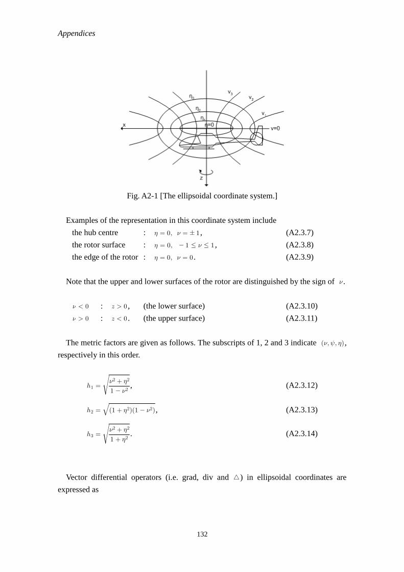
Appendices
132
Fig. A2-1 [The ellipsoidal coordinate system.]
Examples of the representation in this coordinate system include
the hub centre : & = 0, = 1 , (A2.3.7)
the rotor surface : & = 0, 1 1 , (A2.3.8)
the edge of the rotor : & = 0, = 0 . (A2.3.9)
Note that the upper and lower surfaces of the rotor are distinguished by the sign of .
< 0 : z > 0 , (the lower surface) (A2.3.10)
> 0 : z < 0 . (the upper surface) (A2.3.11)
The metric factors are given as follows. The subscripts of 1, 2 and 3 indicate (, ψ, &),
respectively in this order.
h1 =1 22 + &2
√
, (A2.3.12)
h2 = (1 + &2)(1 2)√
, (A2.3.13)
h3 =1 + &22 + &2
√
. (A2.3.14)
Vector differential operators (i.e. grad, div and ) in ellipsoidal coordinates are
expressed as
Appendices
133
gradΦ = e2 + &21 2
√
∂
∂Φ+ eψ
(1 + &2)(1 2)√
1
∂ψ
∂Φ+ e&
2 + &21 + &2
√
∂&
∂Φ ,
(A2.3.15)
divV =2 + &21
∂
∂
(1 2)(2 + &2)√
V1
+∂ψ
∂
(1 + &2)(1 2)√
2 + &2V2
+∂&
∂
(2 + &2)(1 + &2)
√
V3
,
(A2.3.16)
Φ =2 + &21
∂
∂
(1 2)∂
∂Φ
+∂ψ
∂
(1 + &2)(1 2)(2 + &2)
∂ψ
∂Φ
+∂&
∂
(1 + &2)∂&
∂Φ
,
(A2.3.17)
where Φ and V = (V1, V2, V3) are arbitrary scalar and vector functions, respectively.
The differential operators are formally transformed from Cartesian coordinates to
ellipsoidal coordinates as follows,
∂z
∂=h21
1 ∂
∂z ∂
∂+h22
1 ∂ψ
∂z ∂ψ
∂+h23
1 ∂&
∂z ∂&
∂
= 2 + &2&(1 2)
∂
∂ 2 + &2(1 + &2)
∂&
∂, (A2.3.18)
∂x
∂=h21
1 ∂
∂x ∂
∂+h22
1 ∂ψ
∂x ∂ψ
∂+h23
1 ∂&
∂x ∂&
∂
=2 + &2(1 2)
1 21 + &2
√
cos ψ∂
∂+
(1 2)(1 + &2)√
sinψ
∂ψ
∂ 2 + &2&(1 + &2)
1 + &21 2
√
cos ψ∂&
∂,
(A2.3.19)
∂y
∂=h21
1 ∂
∂y ∂
∂+h22
1 ∂ψ
∂y ∂ψ
∂+h23
1 ∂&
∂y ∂&
∂
= 2 + &2(1 2)
1 21 + &2
√
sinψ∂
∂+
(1 2)(1 + &2)√
cos ψ
∂ψ
∂+2 + &2(1 + &2)
1 + &21 2
√
sinψ∂&
∂.
(A2.3.20)
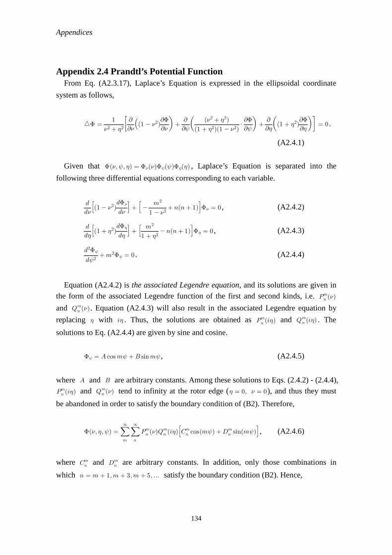
Appendices
134
Appendix 2.4 Prandtl’s Potential Function From Eq. (A2.3.17), Laplace’s Equation is expressed in the ellipsoidal coordinate
system as follows,
Φ =2 + &21
∂
∂
(1 2)∂
∂Φ
+∂ψ
∂
(1 + &2)(1 2)(2 + &2)
∂ψ
∂Φ
+∂&
∂
(1 + &2)∂&
∂Φ
= 0 .
(A2.4.1)
Given that Φ(, ψ, &) = Φ()Φψ(ψ)Φ&(&) , Laplace’s Equation is separated into the
following three differential equations corresponding to each variable.
d
d[
(1 2)d
dΦ]
+[
1 2m2
+ n(n + 1)]
Φ = 0 , (A2.4.2)
d&
d[
(1 + &2)d&
dΦ&]
+[
1 + &2m2
n(n + 1)]
Φ& = 0 , (A2.4.3)
dψ2d2Φψ
+m2Φψ = 0 . (A2.4.4)
Equation (A2.4.2) is the associated Legendre equation, and its solutions are given in the form of the associated Legendre function of the first and second kinds, i.e. Pmn ()
and Qmn (). Equation (A2.4.3) will also result in the associated Legendre equation by
replacing & with i& . Thus, the solutions are obtained as Pmn (i&) and Qmn (i&) . The
solutions to Eq. (A2.4.4) are given by sine and cosine.
Φψ = A cosmψ +B sinmψ , (A2.4.5)
where A and B are arbitrary constants. Among these solutions to Eqs. (2.4.2) - (2.4.4),
Pmn (i&) and Qmn () tend to infinity at the rotor edge (& = 0, = 0), and thus they must
be abandoned in order to satisfy the boundary condition of (B2). Therefore,
Φ(, &, ψ) =∑
m
∞ ∑
n
∞Pmn ()Q
mn (i&)
[
Cmn cos(mψ) +Dmn sin(mψ)
]
, (A2.4.6)
where Cmn and Dm
n are arbitrary constants. In addition, only those combinations in
which n = m + 1, m + 3, m + 5, ... satisfy the boundary condition (B2). Hence,
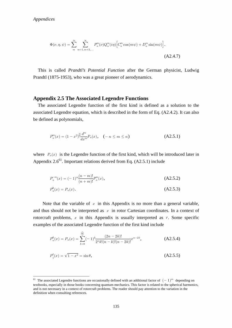
Appendices
135
Φ(, &, ψ) =∑
m
∞ ∑
m+1,m+3,...
∞Pmn ()Q
mn (i&)
[
Cmn cos(mψ) +Dmn sin(mψ)
]
.
(A2.4.7)
This is called Prandtl’s Potential Function after the German physicist, Ludwig
Prandtl (1875-1953), who was a great pioneer of aerodynamics.
Appendix 2.5 The Associated Legendre Functions The associated Legendre function of the first kind is defined as a solution to the
associated Legendre equation, which is described in the form of Eq. (A2.4.2). It can also
be defined as polynomials,
Pmn (x) = (1 x2)2m
dxmdmPn(x), ( n m n) (A2.5.1)
where Pn(x) is the Legendre function of the first kind, which will be introduced later in
Appendix 2.661. Important relations derived from Eq. (A2.5.1) include
Pmn (x) = ( 1)m
(n +m)!
(n m)!Pmn (x), (A2.5.2)
P0n(x) = Pn(x). (A2.5.3)
Note that the variable of x in this Appendix is no more than a general variable,
and thus should not be interpreted as x in rotor Cartesian coordinates. In a context of
rotorcraft problems, x in this Appendix is usually interpreted as r. Some specific
examples of the associated Legendre function of the first kind include
P0n(x) = Pn(x) =∑
k=0
[2
n]
( 1)k2nk!(n k)!(n 2k)!
(2n 2k)!xn2k, (A2.5.4)
P11(x) = 1 x2
√= sin >, (A2.5.5)
61 The associated Legendre functions are occasionally defined with an additional factor of ( 1)m depending on textbooks, especially in those books concerning quantum mechanics. This factor is related to the spherical harmonics, and is not necessary in a context of rotorcraft problems. The reader should pay attention to the variation in the definition when consulting references.
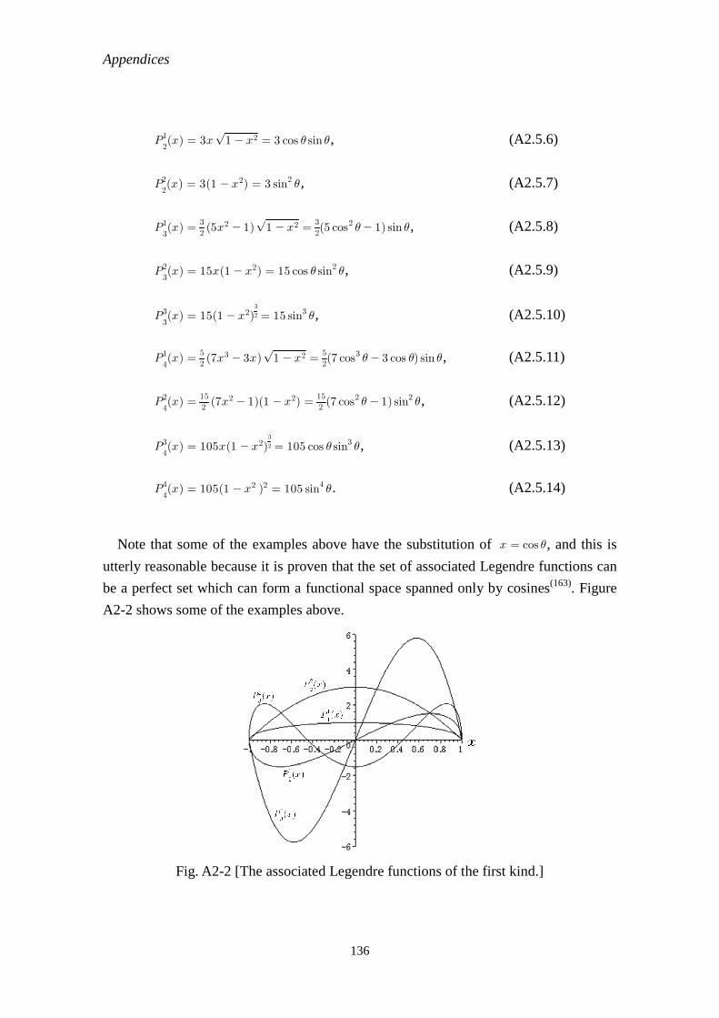
Appendices
136
P12(x) = 3x 1 x2
√= 3 cos > sin >, (A2.5.6)
P22(x) = 3(1 x2) = 3 sin2 >, (A2.5.7)
P13(x) =
2
3(5x2 1) 1 x2
√=
2
3(5 cos2 > 1) sin >, (A2.5.8)
P23(x) = 15x(1 x2) = 15 cos > sin2 >, (A2.5.9)
P33(x) = 15(1 x2)2
3
= 15 sin3 >, (A2.5.10)
P14(x) =
2
5(7x3 3x) 1 x2
√=
2
5(7 cos3 > 3 cos >) sin >, (A2.5.11)
P24(x) =
2
15(7x2 1)(1 x2) =
2
15(7 cos2 > 1) sin2 >, (A2.5.12)
P34(x) = 105x(1 x2)2
3
= 105 cos > sin3 >, (A2.5.13)
P44(x) = 105(1 x2 )2 = 105 sin4 >. (A2.5.14)
Note that some of the examples above have the substitution of x = cos >, and this is
utterly reasonable because it is proven that the set of associated Legendre functions can
be a perfect set which can form a functional space spanned only by cosines(163). Figure
A2-2 shows some of the examples above.
Fig. A2-2 [The associated Legendre functions of the first kind.]

Appendices
137
It can be seen from the diagram that only those associated Legendre functions in
which m + n 1 mod.2 is satisfied become zero at x = 0 . Thus, only those
combinations of m and n which satisfy m + n 1 mod.2 are to be used in rotor
problems. This property can be more rigorously proven by the following recurrence
formula,
(2n + 1)xPmn = (n +m)Pm
n1 + (nm + 1)Pm
n+1. (A2.5.15)
Equation (A2.5.15) is straightforwardly given by mathematical induction from Eqs.
(A2.5.4) - (A2.5.6). The orthogonality of the associated Legendre function of the first
kind is represented as
∫
1
1
Pmn (x)Pm
l(x)dx =
2n + 1
2 (n m)!(n +m)!
<nl. (A2.5.16)
Thus, the associated Legendre function of the first kind can be normalised as
Pmn () = ( 1)m
mn
Pmn ())
, (A2.5.17)
where
mn = 2n + 1
2 (n m)!(n +m)!
√
. (A2.5.18)
Note that since the radial position on the rotor disc is usually normalised by the rotor
radius, the integral interval used in the rotor analysis is [0, 1] , and hence the following
equations can be useful alternatives to Eqs. (A2.5.16) and (A2.5.18) to define the
orthogonality.
∫
0
1
Pmn (x)Pmn (x)dx = 2
1∫
1
1
Pmn (x)Pmn (x)dx = 2n + 1
2 (n m)!(n +m)!
<nl. (A2.5.19)
mn = 2n + 1
1 (n m)!(n +m)!
√
. (A2.5.20)
The associated Legendre function of the second kind is the conjugate function of the
associated Legendre function of the first kind defined as the conjugate solution of the
associated Legendre function of the first kind to Eq. (A2.4.2). Still, the associated
Legendre function of the second kind alone can be defined as

Appendices
138
Qmn (x) = ( 1)m(1 x2)2
m
dxmdmQn(x). ( n m n) (A2.5.21)
It is known that the differentiation of the associated Legendre function of the second
kind can be represented as a simple recurrence relation,
∂x
∂Qmn (x)
=x2 11
[
nxQmn (x) (m + n)Qm
n1(x)]
. (A2.5.22)
When x = 0 ,
Qmn (0) =
Γ
2
1mn
Γ
2
nm+ 1
2m1223
tan[
2
2(m + n)]
, (A2.5.23)
where Γ is the gamma function defined as
Γ(s) =
∫
0
∞xs1exdx (s > 0). (A2.5.24)
Some specific examples of the associated Legendre function of the second kind
include
Q0
0(x) =
2
1ln1 x1 + x
, (A2.5.25)
Q0
1(x) =
2
xln1 x1 + x 1 , (A2.5.26)
Q0
3(x) =
4
x(5x2 3)ln1 x1 + x
+3
2 2
5x2 , (A2.5.27)
Q1
1(x) =
2 1 x2√
(x2 1) ln1x1+x 2x
, (A2.5.28)
Q1
2(x) =
2 1 x2√
4 6x2 + 3x(x2 1) ln1x1+x
, (A2.5.29)
Q2
2(x) =
2(x2 1)2x(3x2 5) 3(x2 1)2 ln
1x1+x
, (A2.5.30)
Q3
3(x) =
2(1 x2)23
30x5 80x3 + 66x + 15(1 x2)3 ln1x1+x
. (A2.5.31)
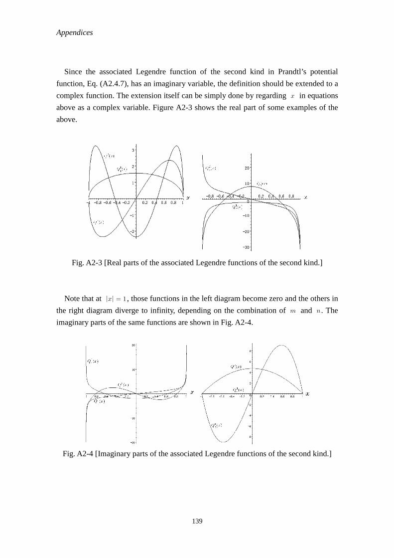
Appendices
139
Since the associated Legendre function of the second kind in Prandtl’s potential
function, Eq. (A2.4.7), has an imaginary variable, the definition should be extended to a
complex function. The extension itself can be simply done by regarding x in equations
above as a complex variable. Figure A2-3 shows the real part of some examples of the
above.
Fig. A2-3 [Real parts of the associated Legendre functions of the second kind.]
Note that at |x| = 1 , those functions in the left diagram become zero and the others in
the right diagram diverge to infinity, depending on the combination of m and n. The
imaginary parts of the same functions are shown in Fig. A2-4.
Fig. A2-4 [Imaginary parts of the associated Legendre functions of the second kind.]

Appendices
140
Appendix 2.6 The Legendre Functions The Legendre functions of the first and second kinds are conjugate solutions to each
other to Legendre’s equation,
(1 x2)dx2d2y 2x
dx
dy+ n(n + 1)y = 0 . (A2.6.1)
The Legendre function of the first kind can be regarded as a special case of the
associated Legendre function, Pmn (x), when m = 0 , yet the Legendre function of the
first kind alone can independently be defined as
Pn(x) =∑
k=0
[2
n]
( 1)k2nk!(n k)!(n 2k)!
(2n 2k)!xn2k. (A2.6.2)
The following recurrence relation is useful.
(2n + 1)xPn(x) = (n + 1)Pn+1(x) + nPn1(x), (n = 1, 2, 3...) (A2.6.3)
where P0(x) = 1 and P1(x) = x . Some specific examples of the Legendre functions of
the first kind include
P0(x) = 1 , (A2.6.4)
P1(x) = x , (A2.6.5)
P2(x) =2
3x2
2
1, (A2.6.6)
P3(x) =2
5x3
2
3x , (A2.6.7)
P4(x) =8
35x4
4
15x2 +
8
3, (A2.6.8)
P5(x) =8
63x5
4
35x3 +
8
15x , (A2.6.9)
P6(x) =16
231x6
16
315x4 +
16
105x2
16
5, (A2.6.10)
P7(x) =16
429x7
16
693x5 +
16
315x3
16
35x . (A2.6.11)
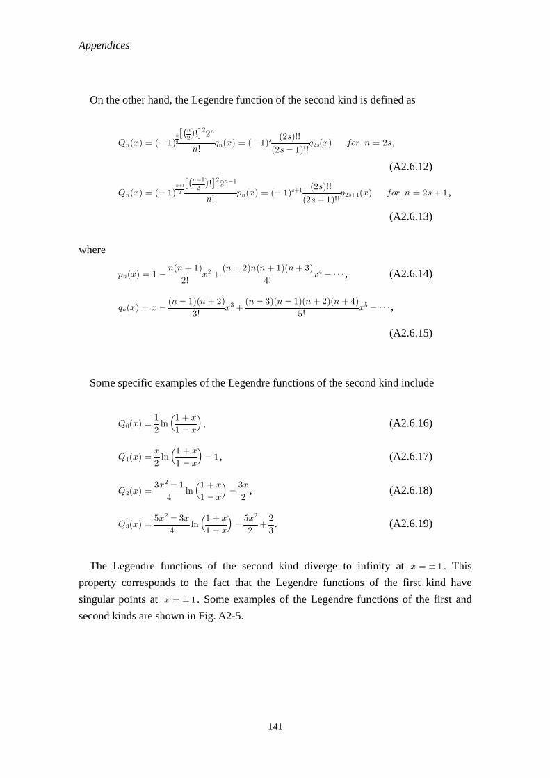
Appendices
141
On the other hand, the Legendre function of the second kind is defined as
Qn(x) = ( 1)2n
n!
*
2
n
!22n
qn(x) = ( 1)s(2s 1)!!(2s)!!
q2s(x) for n = 2s,
(A2.6.12)
Qn(x) = ( 1) 2
n+1
n!
*
2
n1!22n1
pn(x) = ( 1)s+1(2s+ 1)!!
(2s)!!p2s+1(x) for n = 2s+ 1 ,
(A2.6.13)
where
pn(x) = 1 2!
n(n + 1)x2 +
4!
(n 2)n(n + 1)(n + 3)x4 , (A2.6.14)
qn(x) = x 3!
(n 1)(n + 2)x3 +
5!
(n 3)(n 1)(n + 2)(n + 4)x5 ,
(A2.6.15)
Some specific examples of the Legendre functions of the second kind include
Q0(x) =2
1ln
1 x1 + x
, (A2.6.16)
Q1(x) =2
xln
1 x1 + x
1 , (A2.6.17)
Q2(x) =4
3x2 1ln
1 x1 + x
2
3x, (A2.6.18)
Q3(x) =4
5x2 3xln
1 x1 + x
2
5x2+3
2. (A2.6.19)
The Legendre functions of the second kind diverge to infinity at x = 1 . This
property corresponds to the fact that the Legendre functions of the first kind have
singular points at x = 1 . Some examples of the Legendre functions of the first and
second kinds are shown in Fig. A2-5.
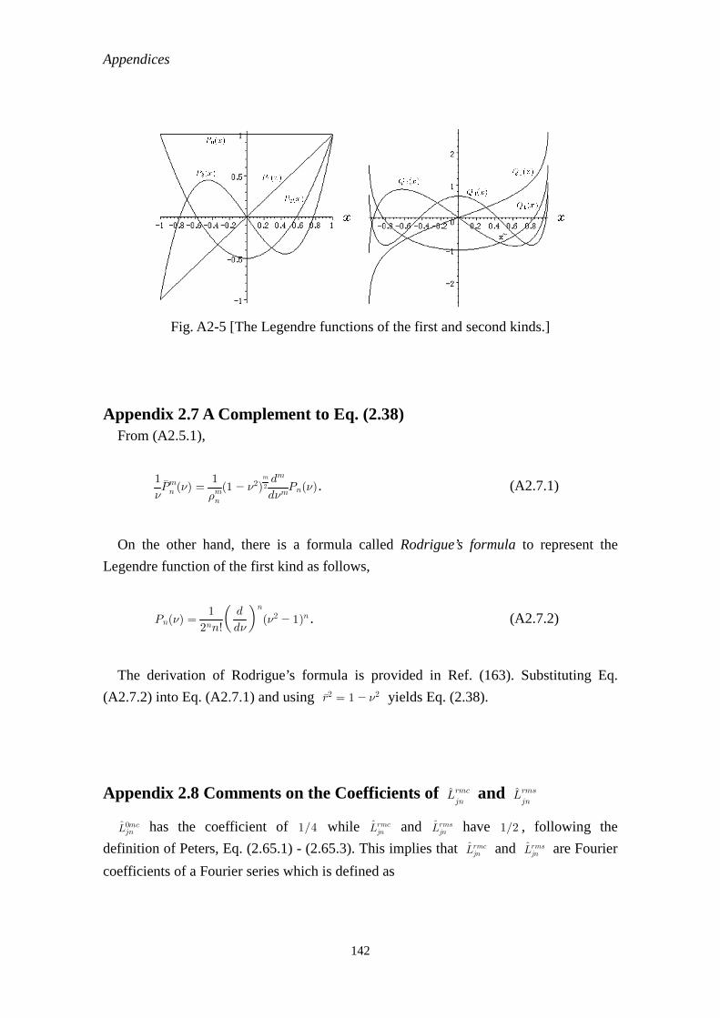
Appendices
142
Fig. A2-5 [The Legendre functions of the first and second kinds.]
Appendix 2.7 A Complement to Eq. (2.38) From (A2.5.1),
1Pmn () = mn
1(1 2)2
m
dmdmPn(). (A2.7.1)
On the other hand, there is a formula called Rodrigue’s formula to represent the
Legendre function of the first kind as follows,
Pn() =2nn!
1
d
dn
(2 1)n . (A2.7.2)
The derivation of Rodrigue’s formula is provided in Ref. (163). Substituting Eq.
(A2.7.2) into Eq. (A2.7.1) and using r2 = 1 2 yields Eq. (2.38).
Appendix 2.8 Comments on the Coefficients of L rmcjn
and L rmsjn
L0mcjn has the coefficient of 1/4 while Lrmcjn and Lrmsjn have 1/2 , following the
definition of Peters, Eq. (2.65.1) - (2.65.3). This implies that Lrmcjn and Lrmsjn are Fourier
coefficients of a Fourier series which is defined as
Appendices
143
f(x) ∑
n=1
∞(an cos nx + bn sinnx), (A2.11.1)
a0 =22
1∫
2
2
f(x)dx , (A2.11.2)
an =2
1∫
2
2
f(x) cos nxdx , (A2.11.3)
bn =2
1∫
2
2
f(x) sinnxdx . (A2.11.4)
where f(x) is an arbitrary periodical functions defined in [ 2, 2] .
In the representations above, while Eq. (A2.11.1) has a pleasing symmetry between
an and bn , the symmetry breaks in Eqs. (A.2.11.2) - (A2.11.4) between a0 and the
others.
There is another definition of Fourier expansion, in which Fourier coefficients are
consistently and symmetrically defined for all n, but the general representation of the
expanded function needs to contain the case selection between n = 0 and n =0 .
f(x) 2
a0+∑
n=1
∞(an cos nx + bn sinnx), (A2.11.5)
an =22
1∫
2
2
f(x) cos nxdx , (A2.11.6)
bn =22
1∫
2
2
f(x) sinnxdx . (A2.11.7)
If the dynamic inflow model were developed based on Eqs. (A2.11.5) - (A2.11.7),
then Eqs. (2.66.1) and (2.66.3) could have been defined in a unified form, but
representations of the pressure potential and induced flow such as Eq. (2.25) must have
had an extra term, for example =0n/2 for Eq. (2.25), in the same form as Eq. (2.11.5).
Many of textbooks including Ref. (163) have Eqs. (A2.11.5) - (A2.11.7) for the
definition of a Fourier series, but Peters used Eqs. (A2.11.1) - (A2.11.4) for his studies.
The variations in the definition should be paid special attention when consulting the
literature.
Appendices
144
Appendix 2.9 Variation in the Representation of the Pressure Potential With regard to the gain matrix elements, in some references such as Ref. (37), Γrm
jn for
r +m 0 mod.2 is given as follows,
Γrmjn=
HmnH
r
j
√( 1) 2
n+j2r
(n + j)(n + j+ 2)[(n j)2 1]
4 (2n + 1)(2j+ 1)√
. (A2.12.1)
Allow Eq. (2.101.1) to be re-carried here again for the comparison,
Γrmjn=
HmnH
r
j
√( 1) 2
n+j2r
(n + j)(n + j+ 2)[(n j)2 1]
2 (2n + 1)(2j+ 1)√
. (2.101.1)
Reference (92) contains Eq. (2.101.1). Equations (2.101.2) and (2.101.3) are also
doubled in Ref. (37). There is also a variation in the representation of the dynamic
inflow model. In Ref. (92), the dynamic inflow model for the cosine part is supposed to
have the form of
[M](a rj) + 2V[Lc]1(ar
j) = (Anmc), (A2.12.2)
while in Ref. (37) it is formulated as
[M](a rj) + V[Lc]1(ar
j) = (Anmc). (A2.12.3)
The reader may notice that the second term in Eq. (A2.12.2) has an extra coefficient
of 2 compared to Eq. (A2.12.3). This variation is due to the variation in the
representation of pressure potential. In Ref. (92), the Fourier coefficients, Amcn , are
associated with the Lift, Eq. (2.13), while in Ref. (37), the Fourier coefficients, Amcn , are
associated with Eq. (2.12). In either way, the induced flow can be associated with the
pressure potential, but depending on how to define the pressure potential and the
dynamic inflow model (i.e. the combination of whether Eqs. (2.12) or (2.13) and
whether Eqs. (A2.12.2) or (A2.12.3)). This thesis is based on the definitions in Ref. (7).
Readers have to avoid the possible confusion when reading a plural of relevant
literature.
Appendices
145
Appendix 3.1 Further Discussion about the Mass-flow Parameter In addition to high-speed flight cases discussed in Subsection 3.2.4, the axial flight
case shall be examined in this Appendix in order to underpin the validity of the
definition of Vm. In axial flight (@ = 0),
VT = ?2√
= |?| (A3.1.1)
in order to maintain CT > 0 . Also,
Vm = |?|?2 + ?m|?|
= ?m + |?f + ?m| . (A3.1.2)
Especially when the vehicle is climbing, as ?f > 0 ,
Vm = 2?m + ?f . (climbing) (A3.1.3)
Likewise, when in descent, as ?f < 0 ,
Vm = ?f . (descent) (A3.1.4)
Note that ?m > 0 in both cases by definition. On the other hand, Peter's definition of
mass-flow parameter, Vm+, yields the following values in axial flight,
Vm+ = 2?m + ?f , (climbing) (A3.1.5)
Vm+ = 2?m ?f . (descent) (A3.1.6)
Since Vm and Vm+ provide the same value with the climbing case, and the sign
change found between Eqs. (A3.1.5) and (A3.1.6) is reflection of the modulus sign
implemented in the definition of Vm, and this is consistent with the observation about
high-speed fligh in Subsection 3.2.4.
Appendices
146
Appendix 3.2 Forces and Moments on a Blade Element The derivation of Eqs. (3.17) and (3.18) are enunciated in this Chapter. References
(5) and (152) should be referred about further details.
The hub velocity vector in aircraft axes, uhub(vehicle) , can be expressed as
uhub(vehicle) = uvehicle(vehicle) +w (rc.g. rhub), (A3.2.1)
where uvehicle(vehicle) is the vehicle velocity in aircraft axes, w is the vehicle angular
velocity, rc.g. is the centre of mass position vector with respect to the airframe reference
and rhub is the position of the rotor hub with respect to the airframe reference.
Then, uhub(vehicle) can be transformed to the shaft-oriented axes, in which the z-axis
lies along the rotor shaft, as
uhub(shaft) = [T1]uhub(vehicle) , (A3.2.2)
where [T1] is the matrix that transforms a vector from airframe to shaft axes defined as
[T1] =
[cos >s 0 sin >s
sin >s sinBs cos Bs sinBssin >s cos Bs sinBs cos >s cos Bs
]
, (A3.2.3)
where >s and Bs are longitudinal and lateral tilt of the rotor shaft with respect to the
airframe, respectively. Next, uhub(shaft) is transformed to a rotating frame of reference
about the shaft,
uhub(hub) = [T2]uhub(shaft) , (A3.2.4)
where uhub(hub) is the hub velocity in the rotating frame of reference and [T2] is defined
as
[T2] =
[
sinψ cos ψ 0cos ψ sinψ 00 0 1
]
, (A3.2.5)
where ψ is the azimuthal position of the reference blade. When the rotor has a
hinge-offset, the hinge velocity, uhinge, is obtained as
Appendices
147
uhinge = uhub(hub) +whinge rhinge+
00
vi
)
, (A3.2.6)
where whinge is the hinge angular velocity, rhinge is the hinge position with respect to
the shaft-based rotating frame of reference and vi is the induced velocity. Note that vi
is a function of radial and azimuthal positions. The hinge angular velocity can be given
as follows;
whinge = [T2][T1]w +
00Ω
)
, (A3.2.7)
where Ω is the rotor speed. By using a transformation matrix, [T3] , that transforms a
vector from hinge to blade axes, we have
wblade = [T3]whinge+
;
>
=
)
, (A3.2.8)
where ;, > and = are flap, pitch and lag angles, respectively, and
[T3] =
[cos = sin = 0
cos ; sin = cos ; cos = sin;sin; sin = cos = sin; cos ;
]
. (A3.2.9)
The absolute velocity of the blade element in the blade axes, ublade, is thus defined as
ublade = uhinge+wblade rbladeelem. , (A3.2.10)
where rbladeelem is the radial position of the blade element with respect to the hinge in
the blade axes. Then, the local angle of attack and the local absolute velocity at the
blade element are calculated as
:elem = >elem + tan1
ublade t(0, 0, 1)ublade t(0, 0, 1), (A3.2.11)
Velem = (ublade t(0, 0, 1))2 + (ublade t(1, 0, 0))2√
. (A3.2.12)
The local lift and drag are defined as
Appendices
148
Lelem =2
1celemV
2
elemrelema:elem, (A3.2.13)
Delem =2
1celemV
2
elemrelem<, (A3.2.14)
where celem is the chord of the blade element, relem is the radial length of the blade
element, a is the lift curve slope and < is the drag coefficient. Note that celem is
generally a function of the radial position, and a and < are generally functions of the
local angle of attack and the local Mach number.
The local lift and drag are defined along the direction of Velem. In the blade element
frame of reference, they are expressed as
Xaero
elem= Lelem sin:elem Delem cos :elem, (A3.2.15)
Yaeroelem
= 0, (A3.2.16)
Zaeroelem
= Lelem cos :elem Delem sin:elem. (A3.2.17)
These are aeronautical loads working on a blade element. On the other hand, the
inertial loads on the blade elements can be given as
Xinertial
elem= melema
elem
elem, (A3.2.18)
where melem is the mass of the blade element and aelem
elem is the absolute acceleration of
the blade element defined as
aelem
elem= [T3]
[T2][T1][
u + w u+w (w rhub)]
+whinge rhinge+wblade [T3](whinge rhinge)
.
(A3.2.19)
Equations (3.17) and (3.18) can be obtained from equations above by defining that
Xelem = Xaero
elem+X
inertial
elem.
References
149
References
N.b.) Although highly convenient, the Internet is not as reliable a source of information
as reviewed papers. Still, it is difficult to completely ignore electric on-line references
available nowadays. The present author dares to include in the reference list a limited
number of websites, which the author judges are relatively sustainable and reliable, for
only supplementary information. It must be herein emphasised that this thesis essentially
relied only on reviewed published papers.
1. Pitt, D.M. and Peters, D.A., “Theoretical Prediction of Dynamic-Inflow
Derivatives,” Vertica, Vol.5, No.1, Jan. 1981, pp.21-34
2. De La Cierva, J., “The Development of the Autogyro,” Journal of Royal
Aeronautical Society, 1926, Vol.30, No.181, pp.8-29
3. De La Cierva, J., “The Autogiro,” Journal of the Royal Aeronautical Society, Vol.34,
No.239, 1930, pp.902-921
4. De La Cierva, J., “New Development of the Autogiro,” Journal of the Royal
Aeronautical Society, Vol.39, Dec. 1935, pp.1125-1143
5. Bramwell, A.R.S., Helicopter Dynamics, Arnold, London, 1976
6. Peters, D.A. and Chen, S.Y., “Momentum Theory, Dynamic Inflow and the
Vortex-Ring State,” Journal of the American Helicopter Society, Jul. 1982, pp.18-24
7. He, C.-J., “Development and Application of a Generalized Dynamic Wake Theory
for Lifting Rotors,” Ph.D. dissertation, Georgia Inst. of Tech, 1989
8. Coton, F.N., Smrcek, L. and Pátek, Z., „Aerodynamic Characteristics of a Gyroplane
Configuration,“ Journal of Aircraft, Vol.35, No.2, Mar.-Apr. 1998
9. Houston, S.S., “Modelling and Analysis of Helicopter Flight Mechanics in
Autorotation,” Journal of Aircraft, Vol.40, No.4, Jul.-Aug. 2003
10. Houston, S.S., “Analysis of Rotorcraft Flight Dynamics in Autorotation,” Journal of
Guidance, Control and Dynamics, Vol.25, No.1, Jan.-Feb. 2002, pp.33-39
11. The United Kingdom Air Accident Investigation Branch.
Webpage: http://www.aaib.dft.gov.uk/home/index.cfm
12. Secretariat of the Aircraft and Railway Accident Investigation Commission of Japan,
Printed reports available from: Ministry of Land, Infrastructure and Transport, 2-1-2,
kasumigaseki, Chiyoda-ku, Tokyo, 100-8919, Japan.
Electric forms available from: http://araic.assistmicro.co.jp/araic/aircraft/
13. Focke, E.H.H., “German Thinking on Rotor Wing Development,” Journal of
Aeronautical Society, Vol.69, No.653, 1965, pp.293-305
References
150
14. Focke, E.H.H., “The Focke Helicopter,” Journal of Aeronautical Society, Vol.42,
May. 1938, pp.577-590
15. Prouty, R.W., Helicopter Aerodynamics, PJS Publications Inc., 2003
16. Wheatley, J.B., “An Aerodynamic Analysis of the Autogiro Rotor with a Comparison
Between Calculated and Experimental Results,” NACA Report No.487, 1937
17. Wheatly, J.B., “Wing Pressure Distribution and Rotor-Blade Motion of an Autogiro
as Determined in Flight,” NACA Report No.475, 1933
18. Wheatly, J.B., “The Aerodynamic Analysis of the Gyroplane, Rotating-Wing
System,” NACA Report No.492, 1934
19. Wheatly, J.B., “Lift and Drag Characteristics and Gliding Performance of an
Autogiro as Determined in Flight,” NACA Report No.434, 1932
20. Lock, C.N.H. and Townend, H.C.H., “Wind Tunnel Experiments on a Model
Autogyro at Small Angles of Incidence,” Aeronautical Research Committee, R&M
1154, Mar. 1927
21. Lock, C.N.H., “Further Development of Autogyro Theory Parts I & II,” Aeronautical
Research Committee, R&M 1127, Mar. 1927
22. Lock, C.N.H, Bateman, H. and Townend, H.C.H., “An Extension of the Vortex
Theory of Airscrews with Applications to Airscrews of Small Pitch, Including
Experimental Results,” R&M. No.1014, British A.R.C., 1926
23. Schad, J.L., “Small Autogyro Performance,” Journal of the American Helicopter
Society, Vol.10, 1965
24. McKillip, R.M. and Chih, M.H., “Instrumented Blade Experiments using a Light
Autogyro,” Proceedings of the 16th European Rotorcraft Forum, Vol.2, The Royal
Aeronautical Society, Glasgow, 1990, pp. 8.4.1-8.4.8
25. Miln-Thomson, L.M., Theoretical Hydrodynamics, Dover Publication Inc.
26. Landau, L.D., Fluid Mechanics, Butterworth-Heinemann, 1987
27. Ormiston, R.A., “An Actuator Disc Theory for Rotor Wake Induced Velocities,”
AGARD Conference Proceedings, AGARD CP. cp.111, 1972
28. Chen, R.T., “A Survey of Nonuniform Inflow Models for Rotorcraft Flight
Dynamics and Control Applications,” Vertica, Vol.14, No.2, 1990, pp.147-184
29. Gaonkar, G.H. and Peters, D.A., “Review of Dynamic Inflow Modeling for
Rotorcraft Flight Dynamics,” Vertica, Vo.12, No.3, 1988, pp.213-242
30. Su, A. and Peters D.A., “The Effect of Hidden Dynamic States on Floquet
Eigenvalues,” Journal of the American Helicopter Society, TN, Vol.35, No.4, Oct.
1990
31. Lowis, O.J., “The Stability of Rotor Blade Flapping Motion at High Tip Speed
References
151
Ratios,” Reports and Memoranda No.3544, Jan. 1963
32. Peters, D.A. and Hohenemser, K.H., “Application of the Floquet Transition Matrix to
Problems of Lifting Rotor Stability,” Journal of the American Helicopter Society,
Vol. 16, No.2, Apr. 1971
33. Gaonkar, G.H. and Peters, D.A., “Review of Floquet Theory in Stability and
Response Analyses of Dynamic Systems with Periodic Coefficients,” Bisplinghoff
Honorary Symposium, Boca Raton, Florida, Feb. 1986
34. Houston, S.S. and Tarttelin, P.C., “Validation of Mathematical Simulations of
Helicopter Vertical Response Characteristics in Hover,” Journal of the American
Helicopter Society, Vol.36, No.1, 1991, pp.45-57
35. Ellenrieder, T.J., “Investigation of the Dynamic Wake of a Model Rotor,” Ph.D.
dissertation, University of Bristol, Oct. 1995
36. Chen, R. T. N. and Hindson, W. S., “Influence of Dynamic Inflow Derivatives,”
Vertica, Vol.5, 1987, pp.21-34
37. Peters, D.A. and He, C.-J., “Finite State Induced Flow Models Part II:
Three-Dimensional Rotor Disk,” Journal of Aircraft, Vol.32, No.2, Mar.-Apr., 1995
38. Turnour, S.R. and Celi, R., “Modelling of Flexible Rotor Blades for Helicopter
Flight Dynamics Applications,” Journal of American Helicopter Society, Vol.41,
No.1, 1996, pp.52-61
39. Peters, D.A. and He, C.-J., “A Closed-Form Unsteady Aerodynamic Theory for
Lifting Rotors in Hover and Forward Flight,” the 43rd Annual National Forum of the
American Helicopter Society, Missouri, May. 1987
40. Gaonkar, G.H., et al, ”The Use of Actuator-Disc Dynamic Inflow for Helicopter
Flap-Lag Stability,” Journal of the American Helicopter Society, Vol.28, No.3, Jul.
1983
41. Glauert, H., “A General Theory of the Autogyro,” Reports and Memoranda No.1111,
Aeronaut Res. Council, 1926
42. Brotherhood, P., “An Investigation in Flight of Induced Velocity distribution Under a
Helicopter Rotor When Hovering,” Br. ARCRAE Report No.Aero.2211, Jun. 1947
43. Coleman, R.P., Feingold, A.M, and Stempin, C.W., “Evaluation of the Induced
Velocity Field of an Idealized Helicopter Rotor,” NACA ARR L5E10, 1945
44. Stepniewski, W.Z. and Keys, C.N., Rotary-Wing Aerodynamics, Dover Publication
Inc., 1984
45. Harris, F.D. and McVeigh, M.A., “Uniform Downwash with Rotors Having a Finite
Number of Blades,” Journal of the American Helicopter Society, Vol.21, No.1, Jan.
1976
References
152
46. Harris, F.D., “Articulated Rotor Blade Flapping Motion at Low Advance Ratio,”
Journal of the American Helicopter Society, Vol.17, No.1, Jan. 1972
47. Kinner, W., “Die Kreisfirmige Tragflasche auf Potentialtheorischer Grundlage,”
Ingenier Archive VIII Band, 1937, pp.47-80
48. Mangler, K.W. and Squire, B., “Calculation of the Induced Velocity Field of a
Rotor,” Royal Aircraft Establishment, Rept. Aero 2247, Sep. 1948
49. Joglekar, M. and Loewy, R., “An Actuator Disc Analysis of Helicopter Wake
Geometry and the Corresponding Blade Response,” USAAU-LBS, Tech. Report,
1970
50. Carpenter, P.J. and Friedvich, “Effect of a Rapid Blade-Pitch Increase on the Thrust
and Induced-Velocity Response of a Full-Scale Helicopter Rotor,” NACA TN 3044,
1953
51. Munk, M.M., “Some Tables of the Factors of Apparent Mass,” National Advisory
Committee for Aeronautics, Technical Note NO.197, 1924
52. Castles, W. Jr. and De Leeuw, J.H., “The Normal Component of the Induced Velocity
in the Vicinity of a Lifting Rotor and Some Examples of Its Application,” NACA
Rept. 1184, 1954
53. Heyson, H.H. and Katzoff, S., “Induced Velocities Near a Lifting Rotor with
Nonuniform Disk Loading,” NACA Rept. 1319, 1957
54. Jewel, I.W. and Heyson, H.H., “Charts of the Induced Velocities Near a Lifting
Rotor,” NASA MEMO 4-15-59L, May. 1959
55. Sissingh, G.J., “The Effect of Induced Velocity Variation on Helicopter Rotor
Damping in Pitch or Roll,” TN No.Aero 2132, Nov. 1951
56. Amer, K.B., “Theory of Helicopter Damping in Pitch and Roll and a Comparison
with Flight Measurements,” NACA T.N. 2136, Oct. 1950
57. Brotherhood, P. and Steward, W., “An Experimental Investigation of the Flow
Through a Helicopter Rotor in Forward Flight,” Aeronautical Research Council,
Report and Memoranda No.2734, Sep. 1949
58. Curtiss, H.C. Jr., and Schupe, N.K., “Stability and Control Theory for Hingeless
Rotors,” Ann. Forum AHS, May. 1971
59. Banerjee, D., Crews, S.T., Hohenemser K. and Yin, S., “Identification of State
Variables and Dynamic Inflow from Rotor Model Dynamic Tests,” Journal of the
American Helicopter Society, Vo.22, 1977
60. Kuczynski, W.A. and Sissingh, G.J., “Characteristics of Hingeless Rotors with Hub
Moment Feedback Controls including Experimental Rotor Frequency Response,”
NASA CR 114427 (Vol.1) and CR 114428 (Vol.II), 25048, Jan. 1972
References
153
61. Bousman, W.G., “An Experimental Investigation of the Effects of Aeroelastic
Coupling on Aeromechanical Stability of a Hingeless Rotor Helicopter,” Journal of
the American Helicopter Society, Vol.26, No.1, Jan. 1981, pp.46-54
62. Gaonkar, G.H. and Peters, D.A., “A Review of Dynamic Inflow and Its Effect on
Experimental Correlations,” Second Decennial Specialists’ Meeting on Rotorcraft
Dynamics, AHS-NASA, Ames, Moffet Field, California, Nov. 7-9, 1984
63. Wood, E.R. and Hermes, M.E., “Rotor Induced Velocities in Forward Flight by
Momentum Theory,” AIAA Paper No.69-224, 1969
64. Azuma, A. and Kawachi, K., “Local Momentum Theory and Its Application to the
Rotor Wing,” Journal of Aircraft, Vol.16, No.1, 1979, pp.6-14
65. Ormiston R.A. and Peters, D.A., “Hingeless Helicopter Rotor Response with
Nonuniform Inflow and Elastic Blade Bending,” Journal of Aircraft, Vol.9, No.10,
Oct. 1972
66. Peters, D.A., “Hingeless Rotor Frequency Response with Unsteady Inflow,” NASA
SP-352 Rotorcraft Dynamics, 1974
67. Ormiston, R.A., “Application of Simplified Inflow Model to Rotorcraft Dynamic
Analysis,” Journal of American Helicopter Society, Vol.21, No.3, Jul. 1976
68. Crews, S.T., Hohenemser, K.H. and Ormiston, R.A., “An Unsteady Wake Model for
a Hingeless Rotor,” Journal of Aircraft, Vol.10, No.12, Dec. 1973
69. White, F. and Blade, B.B., “Improved Method of Predicting Helicopter Control
Response and Gust Sensitivity,” Ann. Forum AHS, May. 1979
70. Johnson, W., “Influence of Unsteady Aerodynamics on Hingeless Rotor Ground
Resonance,” Journal of Aircraft, Vol.29, No.9, Aug. 1982
71. Johnson, W., Helicopter Theory, Princeton Univ. Press, 1994
72. Peters, D.A. and Gaonkar, G.H., “Theoretical Flap-Lag Damping with Various
Dynamic Inflow Models,” Journal of the American Helicopter Society, Vol.25, No.3,
Jul. 1980, pp.29-36
73. Banerjee, D., Crews, S.T., Hohenemser K. and Yin, S., “Parameter Identification
Applied to Analytic Hingeless Rotor Modeling,” Journal of the American Helicopter
Society, Vo.24, No.1, Jan. 1979, pp.26-32
74. Gaonkar, G.H., Mitra, A.K. and Peters, D.A., “Feasibility of a Rotor
Flight-Dynamics Model with First Order Cyclic Inflow and Multiblade Modes,”
AIAA Dynamics Specialists’ Conference, Atlanta, Ga., Apr. 1981, AIAA Paper No.
81-0611-CP.
75. Van Holten, Th., “The computation of aerodynamic loads on helicopter blades in
forward flight, using the method of the acceleration potential,” Rep. VTH-189,
References
154
Technische Hogeschool Delft, Netherlands, Mar. 1975
76. Pierce, G.A. and Vaidynathan, A.R., “Helicopter Rotor Loads Using a Matched
Asymptotic Expansion technique,” NASA CR-165742, May. 1981
77. Meijer Drees, J. and Hendal, W.P., “Airflow Patterns in the Neighbourhood of
Helicopter Rotors,” Aircraft Engineering, Vol.23, No.266, Apr. 1951
78. Pitt, D.M., “Rotor Dynamic Inflow Derivatives and Time Constants from Various
Inflow Models,” Ph.D. dissertation, Washington University, Dec. 1989
79. Glauert, H.M.A., “The Force and Moment of an Oscillating Aerofoil,” R.&M.
No.1292 (‘Ae. 397), 1929
80. Theodorsen T., “General Theory of Aerodynamic Instability and the Mechanism of
Flutter,” NACA TR No.496, 1935
81. Isaacs, R., “Airfoil Theory for Rotory Wing Aircraft,” Journal of Aeronautical
Sciences, Vol.13, No.4, Apr. 1945, pp.218
82. Greenberg, J.M., “Airfoil in Sinusoidal Motion in Pulsating Stream,” NACA TN
No.1326, 1947
83. Willmer, M.A.P., “The Loading of Helicopter Blades in Forward Flight,” RAE
Report Naval 20N276935 No. 8, Apr. 1959
84. Brown, R.E. and Houston, S.S., “Comparison of Induced Velocity Models for
Helicopter Flight Mechanics,” AIAA Journal, Vol.37, No.4, 2000, pp.623-629
85. Miller, R.H., “Rotor Blade Harmonic Air Loading,” AIAA Journal, Vol.2, No.7, 1964,
pp.1254-1269
86. Loewy, R.G., “A Two-Dimensional Approximation to the Unsteady Aerodynamics of
Rotary Wings,” Journal of the Aeronautical Sciences, Vol.24, 1957
87. Jones, W.P. and Rao, B.M., “Compressibility Effects on Oscillating Rotor Blades in
Hovering Flight,” AIAA Journal, Vol.8, No.2, 1970, pp.321-329
88. Hammond, C.E. and Pierce, G.A., “A Compressible Unsteady Aerodynamic Theory
for Helicopter Rotors,” AGARD Specialists’ Meeting on the Aerodynamics of
Rotary Wings, Marseille, France, Sep. 13-15, 1972
89. Friedmann, P.P. and Venkatesan, C., “Influence of Various Unsteady Aerodynamic
Models of the Aeromechanical Stability of a Helicopter in Ground Resonance,”
NASA CP-2400, 1985
90. Friedmann, P.P. and Venkatesan, C., “Finite State Modelling of Unsteady
Aerodynamics and Its Application to a Rotor Dynamic Problem,” 11th European
Rotorcraft Forum, Paper No.72, London, Sep. 10-13, 1985
91. Venkatesan, C. and Friedmann, P.P., “New Approach to Finite-State Modelling of
Unsteady Aerodynamics,” AIAA Journal, Vol.24, No.12, 1986 pp.1889-1897
References
155
92. Peters, D.A. and He, C.-J., “Correlation of Measured Induced Velocities with a
Finite-State Wake Model,” Journal of the American Helicopter Society, Vol.36, No.3,
1991, pp.59-70
93. Heyson, H.H., “A Brief Survey of Rotary Wing Induced Velocity Theory,” NASA
TM78741, Jun. 1978
94. Landgrebe, A.J., “An Analytical Method for Predicting Rotor Wake Geometry,”
Journal of the American Helicopter Society, Vol.14, No.4, Oct. 1969
95. Sadler, S.G., “Development and Application of a Method for Predicting Free Wake
Positions and Resulting Rotor Blade Air Loads,” Vol.1 Model and Results, NASA
CR-1011, 1971
96. Padfield, G.D., “Theoretical Modelling for Helicopter Flight Dynamics:
Development and Validation,” International Council for the Aeronautical Sciences,
ICAS-88-6.1.3, Jerusalem, Israel, 1988, pp.165-177
97. Drazin, P.G., Nonlinear System, Cambridge Univ. Press, 1992
98. Basset, P.M., “Study of the Vortex Ring State Using Bifurcation Theory, ” American
helicopter Society 58th Annual Forum, Montreal, Canada, 2002
99. Houston, S.S. and Brown, R.E., “Rotor-Wake Modelling for Simulation of
Helicopter Flight Mechanics in Autorotation,” Journal of Aircraft, Vol.40, No.5, Sep.
2003
100.Faulkner, A.J. and Buchner, F., “Flight Investigations of a Helicopter low airspeed
estimation system based on measurement of control parameters,” 6th European
Rotorcraft Forum, 1980
101.Nagabhushanam, J. and Gaonkar, G.H., “Rotorcraft Air Resonance in Forward Flight
with Various Dynamic Inflow Models and Aeroelastic Couplings,” Vertica, Vol.8,
No.4, 1984, pp.373-394
102.Gaonkar G.H. and Peters, D.A., “Effectiveness of Current Dynamic Inflow Models
in Hover and Forward Flight,” Journal of American Helicopter Society, Vol.31, No.2,
Apr. 1986
103.Siblski, K., “Non-Linear Flight Mechanics of a Helicopter Analysis by Application
of a Continuation Methods,” 20th European Rotorcraft Forum, Rome, Italy, 1999
104.Chen, R. and Hindson, W.S., “Influence of Dynamic Inflow on the Helicopter
Vertical Response,” NASA TM-88327, No. 87-24482, Jun. 1986
105.Pitt D.M. and Peters D.A., “Rotor Dynamic Inflow Derivatives and Time Constants
from Various Inflow Models,” 9th European Rotorcraft Forum, No.55, 1983
106.Pitt, D.M., “Rotor Dynamic Inflow Derivatives and Time Constants from Various
Inflow Models,” USATSARCOM-TR81-2, Dec. 1980
References
156
107.Peters, D.A. and HaQuang, N., “Dynamic Inflow for Practical Applications,”
Journal of the American Helicopter Society, TN, vol.33, No.4, Oct. 1988, pp.64-68
108.Schrage, D.P., Peters D.A. and Prasad, V.R., “Helicopter Stability and Control
Modeling Improvements and Verification,” 14th European Rotorcraft Forum, Part I,
No.77, Milan, 1988
109.Su, A., Yoo, K.M. and Peters, D.A., “Extension and Validation of an Unsteady Wake
Model for Rotors,” Journal of Aircraft, Vol.29, No.3, 1992, pp.374-383
110.Su, A., “Application of a State-Space Wake Model to Elastic Blade Flapping in
Hover,” Ph.D. dissertation, Georgia Inst. of Technology, Atlanta, GA, Dec. 1989
111.De Andrade, D. and Peters, D.A., “Correlation of Experimental Flap-Lag Torsion
Damping - A Case Study,” Proceedings of the 49th Annual National Forum of the
American Helicopter Society, St. Louis, 1993, pp.1011-1028
112.Peters, D.A., Boyd, D.D. and He, C.-J., “Finite-State Induced-Flow Model for
Rotors in Hover and Forward Flight,” Journal of the American Helicopter Society,
Vol. 34, No.4, 1989, pp.5-17
113.Nibbelink, B.D. and Peters, D.A., “Flutter Calculations for Fixed and Rotating Wing
with State-Space Inflow Dynamics,” Proceedings of AIAA/AHS/ASME Structural
Dynamics and Materials Conference, La Jolla, Apr. 1993
114.Elliot, J.W., Althoff S.L. and Sailey, R.H., “Inflow Measurements Made with a Laser
Velocimeter in Forward Flight, Volume 3, Rectangular Planform Blades at an
Advance Ratio of 0.15,” NASA TM 100541, AVSCOM TM 88-B-004, Apr. 1984
115.Elliot, J.W., Althoff S.L. and Sailey, R.H., “Inflow Measurements Made with a Laser
Velocimeter in Forward Flight, Volume 3, Rectangular Planform Blades at an
Advance Ratio of 0.23,” NASA TM 100542, AVSCOM TM 88-B-005, Apr. 1984
116.Elliot, J.W., Althoff S.L. and Sailey, R.H., “Inflow Measurements Made with a Laser
Velocimeter in Forward Flight, Volume 3, Rectangular Planform Blades at an
Advance Ratio of 0.30,” NASA TM 100543, AVSCOM TM 88-B-006, Apr. 1984
117.Xin, H., Prasad, J.V.R. and Peters, D.A., “Dynamic Inflow Modelling for Simulation
of a Helicopter Operating in Ground Effect,” AIAA Modeling and Simulation
Technologies Conference and Exhibit, Portland, OR, Collection of Technical Papers,
Aug. 9-11, 1999, pp.182-192
118.Xin, H., Prasad, J.V.R. and Peters, D.A., “Ground Effect Aerodynamics of Lifting
Rotors Hovering above Inclined Ground Plane,” the AIAA 17th Applied
Aerodynamics Conference, Norfolk, VA, Jun. 1999
119.Takahashi, M.D., “A Flight Dynamic Helicopter Mathematical Model with a Single
Flap-Lag-Torsion Main Rotor,” NASA TM 102267, USAAVSCOM TM 90A004,
References
157
Feb. 1990
120.Chaimovitch, M., Rosen, A., Mansur, M.H. and Tschler, M.B., “Investigation of the
Flight Mechanics Simulation of a Hovering Helicopter,” the 48th Annual Forum of
the American Helicopter Society, Washington D.C., Jun. 1999, pp.1237-1256
121.He, C.-J. and Lewis, W.D., “A Parametric Study of Real-Time Mathematical
Modeling Incorporating Dynamic Wake and Elastic Blades,” the 48th Annual Forum
of the American Helicopter Society, Washington D.C., Jun. 1999, pp.1181-1196
122.Harding, J.W. and Bass, S.M., “Validation of a Flight Simulation Model of the
AH-64 Apache Attack Helicopter against Flight Test Data,” the 46th Annual Forum
of the American Helicopter Society, Washington D.C., May. 1990
123.Prouty, R.W., “The Case of the Cross-Coupling Mystery,” Rotor and Wing, Vol.28,
No.6, 1994, pp.48-49
124.Von Grünhagen, W., “Dynamic Inflow Modelling for Helicopter Rotors and Its
Influence on the Prediction of Cross-Couplings,” Proceedings of the AHS
Aeromechanics Specialists Conference, Bridgeport, CT, Oct. 1995
125.Ballin, M.G. and Dalang-Secretan, M.A., “Validation of the Dynamic Response of a
Blade-Element UH-60 Simulation Model in Hovering Flight,” Proceedings of the
American Helicopter Society 46th Annual Forum, Washington D.C., May. 1990
126.Simons, I.A. and Modha, A.N., “Gyroscopic Feathering Moments and the Bell
Stabilizer Bar on Helicopter Rotors,” the 2002 European Rotorcraft Forum, Bristol,
England, Sep. 17-20, 2002, pp.90.1-90.8
127.Rosen, A. and Isser, A., “A New Model of Rotor Dynamics During Pitch and Roll of
a Hovering Helicopter,” Journal of the American Helicopter Society, Vol.40, No.3,
Jul.1995, pp.17-28
128.Rosen, A. and Isser, A., “A Model of the Unsteady Aerodynamics of a Hovering
Helicopter Rotor that Includes Variations of the Wake Geometry,” Journal of the
American Helicopter Society, Vol.40, No.3, Jul.1995, pp.6-16
129.Krothapalli, K.R., Prasa, J.V. and Peters, D.A., “Helicopter Rotor Dynamic Inflow
Modeling for Maneuvering Flight,” Journal of the American Helicopter Society,
2001, Apr. pp129-139
130.Barocela, E.B., Peters, D.A., Krothapalli, K.R. and Prasad, J.V.R., “The Effect of
Wake Distortion on Rotor Inflow Gradients and Off-Axis Coupling,” Proceedings of
the Atmospheric Flight Mechanics Conference of the American Institute of
Aeronautics and Astronautics, New Orleans, Louisiana, Aug. 1997
131.Krothapalli, K.R., Prasa, J.V. and Peters, D.A., “Improved Wake Geometry Model
for a Maneuvering Rotor,” Proceedings of the American Helicopter Society
References
158
Technical Specialists’ Meeting for Rotorcraft acoustics and Aerodynamics,
Williamsburg, Virginia, Oct. 1997
132.Krothapalli, K.R., Prasa, J.V. and Peters, D.A., “Development of a Comprehensive
Wake Theory for Lifting Rotors,” Proceedings of the Atmospheric Flight Mechanics
Conference of the American Institute of Aeronautics and Astronautics, San Diego,
California, Jul. 1996
133.He, C.-J., Lee, C.-S. and Chen, W., “Rotorcraft Simulation Model Enhancement to
Support Design, Testing and Operational Analysis,” the American helicopter Society
55th Annual Forum, Montreal, Canada, May 25-27, 1996
134.Zhao, J.-G., Prasad, J. and Peters, D.A., “Simplified Dynamic Wake Distortion
Model for Helicopter Transitional Flight,” AIAA Atmospheric Flight Mechanics
Conference and Exhibit, Monterey, California, Aug. 5-8, 2002
135.Zhao, J.-G., “Dynamic Wake Distortion Model for Helicopter Maneuvering Flight,”
Ph.D. dissertation, Georgia Inst. of Technology, Atlanta, GA, Mar. 2005
136.Peters, D.A. and Morillo, J.A., “Towards a Complete Dynamic Wake Model in Axial
Flow,” Proceedings of the American Helicopter Society Aeromechanics Specialists’
Meeting, Atlanta, Georgia, Nov. 13-14, 2000
137.Morillo, J. and Peters, D.A., “Extension of Dynamic Inflow Models to Include Mass
Injection and Off-disk Flow,” AIAA Aerospace Sciences Meeting and Exhibit, 40th,
Reno, Jan. 14-17, 2002
138.De La Cierva, J., “A Letter to RAeS with Comments on the Paper Presented by H.
Glauert on 20 January 1927,” Journal of the Royal Aeronautical Society, Vol.31,
No.198, 1927, pp.5060-506
139.Beavan, J.A. and Lock, C.N.H., “The Effect of Blade Twist on the Characteristics of
the C-30 Autogyro,” Aeronautical Research Council, ARC R&M 1727, London,
1939
140.Glauert, H., “Lift and Torque of an Autogyro on the Ground,” Aeronautical Research
Committee, R&M 1131, Jul. 1927
141.Glauert H. and Lock, C.N.H., “A Summary of the Experimental and Theoretical
Investigations of the Characteristics of an Autogyro,” Aeronautical research
Committee R&M 1162, Apr. 1928
142.Glauert, H., “The Analysis of Experimental Results in the Windmill Brake and
Vortex Ring States of an Airscrew,” R&M. No.1026, British A.R.C., 1926
143.Glauert, H., “The Theory of the Autogiro,” Journal of the Royal Aeronautical
Society, Vol.31, No.198, 1927, pp.483-505
144.Moreno-Caracciolo, M, “The Autogiro,” Technical Memorandum No.216, 1923

References
159
145.Leishman, J.G., “Development of the Autogiro: A Technical Perspective,” AIAA
Journal, 0021-8669 Vol.41, No.4, 2004
146.Popular Rotorcraft Association. Webpage: http://www.pra.org
147.Ken Wallis’ personal webpage: http://www.kenwallisautogyro.com
148.Anon, “British Civil Airworthiness Requirements Section T: Light Gyroplane design
Requirements,” U.K. Civil Aviation Authority, Paper T860, Jul. 1993
149.Houston S.S., “Identification of Gyroplane Lateral/Directional Stability and Control
Characteristics from Flight Test,” Proceedings of the Institute of Mechanical
Engineers, Pt. G, Vol.212, No. G4, 1998, pp.1-15
150.Houston, S.S., “Longitudinal Stability of Gyroplanes,” The Aeronautical Journal of
the Royal Aeronautical Society, Jan. 1996
151.Houston, S.S. and Brown, R.E., “Rotor-Wake Modelling for Simulation of
Helicopter Flight Mechanics in Autorotation,” Journal of Aircraft, Vol.40, No.5, Sep.
2003, pp.938-945
152.Houston, S.S., “Validation of a Non-linear Individual Blade Rotorcraft Flight
Dynamics Model Using a Perturbation Method,” Aeronautical Journal, Aug.-Sep.
1994, pp.260-266
153.Houston, S.S. and Tarttelin, P.C., “Validation of Mathematical Simulations of
Helicopter Vertical Response Characteristics in Hover,” Journal of the American
Helicopter Society, Vol.36, No.1, 1991, pp.45-57
154.Spathopoulos, V.M., “The Assessment of a Rotorcraft Simulation Model in
Autorotation by Means of Flight Testing a Light Gyroplanes,” Ph.D. dissertation.
Dept. of Aerospace Engineering, Univ. of Glasgow, Scotland U.K., Aug. 2001
155.Bagiev, M., “Gyroplane handling Qualities Assessment Using Flight Testing and
Simulation Technique,” Ph.D. dissertation. Dept. of Aerospace Engineering, Univ. of
Glasgow, Scotland U.K., Aug. 2005
156.Carter Jr. J., “The Carter Heliplane Transport Slowed/Compound Aircraft: Candidate
for the Air-Maneuver Transport(AMT),” Carter Aviation Technologie.
Webpage: http://www.cartercopters.com/
157.Groen Brothers Aviation Incorporated. Company.
Webpage: http://www.groenbros.com
158.PAL-V Europe BV. Webpage: http://www.pal-v.com/
159.Lopez, C.A. and Wells, V.L., “Dynamic and Stability of an Autorotating Rotor/Wing
Unmanned Aircraft,” Journal of Guidance, Control, and Dynamics, Vol.27, No.2,
Mar.-Apr. 2004, pp.258-270
160.Skews, B.W., “Autorotation of Rectangular Plates,” J. Fluid Mech. Vol. 217, 1990,
References
160
pp.33-40
161.Lugt, H.J., “Autorotation,” Ann. Rev. Fluid Mech. 1983, 15:123-47
162.Hislop, G.S., “The Fairy Rotordyne,” Meetings of the Helicopter Association of
Great Britain &The Royal Aeronautical Society, London, Nov. 1958
163.Arfken, G.. and Weber, H., Mathematical Methods for Physicists, 3rd ed. Academic
Press, 1995
164.Mathworld Website: http://mathworld.wolfram.com/
165.Abramovich, M. and Stegun, I., Handbook of Mathematical Functions, Dover
Publications, Inc., 1972
166.Peters, D.A. and Cao, W.M., “Finite State Induced Flow Models Part I:
Two-Dimensional Thin Airfoil,” Journal of Aircraft, Vol.32, No.2, Mar.-Apr. 1995
167.The Wolfram Functions Site. Webpage: http://functions.wolfram.com/
168.Murakami, Y. and Houston, S., “Dynamic inflow modelling for autorotating rotors”
Aeronautical Jouranal, Vol.112, No.1127, Jan. 2008, pp 47-53
169.Peters, D.A. and He, C.-J., “Modification of Mass-Flow Parameter to Allow Smooth
Transition Between Helicopter and Windmill States,” Journal of the American
Helicopter Society, TN, 51, No 3, Jul. 2006, pp.275-278
170.He, C.-J., Lee, C.-S. and Chen, W., “Finite State Induced Flow Model in Vortex Ring
State,” Journal of the American Helicopter Society, TN, 45, No 4, Oct. 2000,
pp.318-320
171.Padfield, G.D., Helicopter Flight Dynamics, Blackwell Science, Oxford, 1996
172.Done, G. and Balmford, D., Bramwell's Helicopter Dynamics, 2nd ed. Butterworth
Heinemann, 2001
173.Leishman, J.D., Principles of Helicopter Aerodynamics, 2nd ed. Cambridge
University Press, 2006
174.Abbott, P.B., The Gyroplane Flight Manual, Abbott Co., 1996
175. Abbott, P.B., Understanding the Gyroplane, Abbott Co., 1994
176. Mangler, K.W., “Fourier Coefficients for Downwash at a Helicopter Rotor,” R.A.E.
Technical Note No. Aero. 1958, May, 1948