Digital Communications Through Fading Multipath Channels

EE 573 Digital Communication II

Dr. Ali Muqaibel

Basic Questions

Desert Metro Street Indoor

What will happen if the transmitter- changes transmit power ?- changes frequency ?- operates at higher speed ?

What will happen ifthe receiver moves?

What will happen if we conduct this experiment in different types of environments?

Channel efffects

Effect of mobility

Transmit power, data rate, signal bandwidth, frequencytradeoff

Tx

Rx

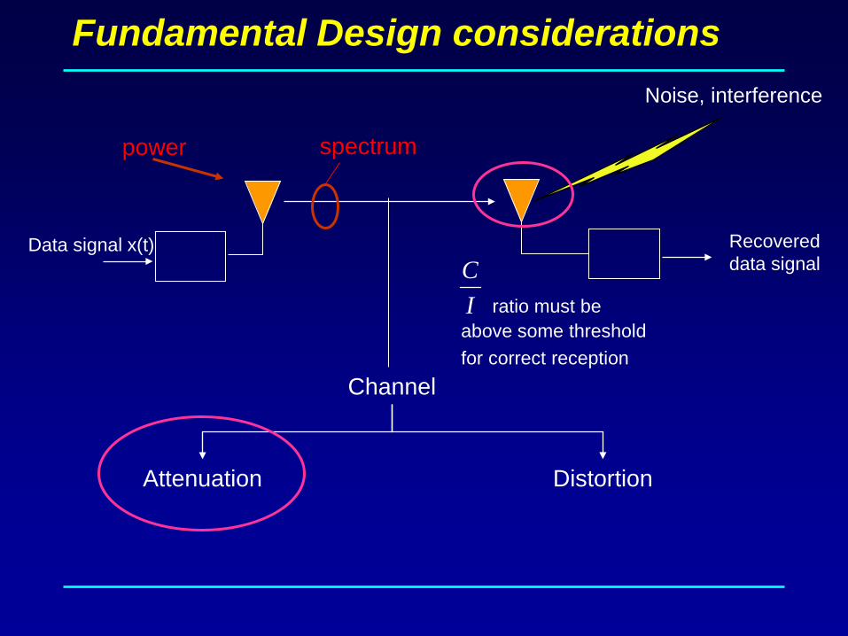
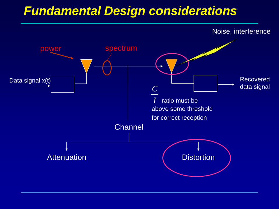
Fundamental Design considerations

Data signal x(t) Recovereddata signal

power spectrum

Noise, interference

ratio must beabove some thresholdfor correct reception

IC

Channel

Attenuation Distortion

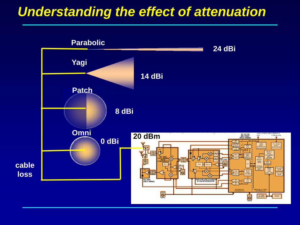
Understanding the effect of attenuation

Parabolic

Yagi

Patch

Omni

24 dBi

14 dBi

8 dBi

0 dBi 20 dBm

cableloss

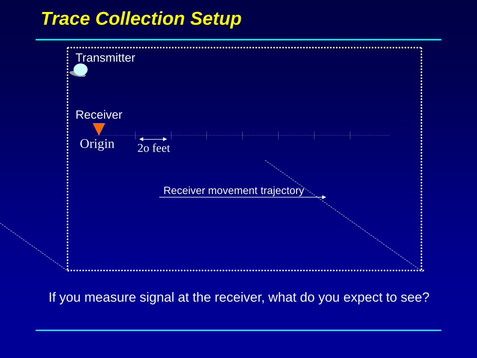
Trace Collection Setup

Receiver

Transmitter

Receiver movement trajectory

Origin 2o feet

If you measure signal at the receiver, what do you expect to see?

Measured Signal

Signal Strength

-80

-70

-60

-50

-40

-30

-20

-10

0

Time

dBm

Channel 4 Avg. Signal Strength

+20 feet +20 feet +20 feet +20 feet +20 feet +20 feet +20 feetOrigin

Long range path lossSmall scale fading

Fundamental Design considerations

Data signal x(t) Recovereddata signal

power spectrum

Noise, interference

ratio must beabove some thresholdfor correct reception

IC

Channel

Attenuation Distortion

Radio Propagation: Fading and multipath

Tx

Rx

Fading: rapid fluctuation of the amplitude of a radio signal over a short period of time or travel distance

• Fading• Varying doppler shifts on different multipath signals• Time dispersion (causing inter symbol interference)

Effects of multipath

Review of basic concepts

Fourier Transform Channel Impulse response Power delay profile Inter Symbol Interference Coherence bandwidth Coherence time

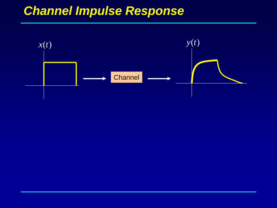
Channel Impulse Response

)(tx

Channel

)(ty

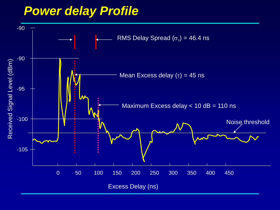
Power delay ProfileR

ecei

ved

Sig

nal L

evel

(dB

m)

-105

-100

-95

-90

-90

0 50 100 150 200 250 300 350 400 450

Excess Delay (ns)

RMS Delay Spread (στ) = 46.4 ns

Mean Excess delay (τ) = 45 ns

Maximum Excess delay < 10 dB = 110 ns

Noise threshold

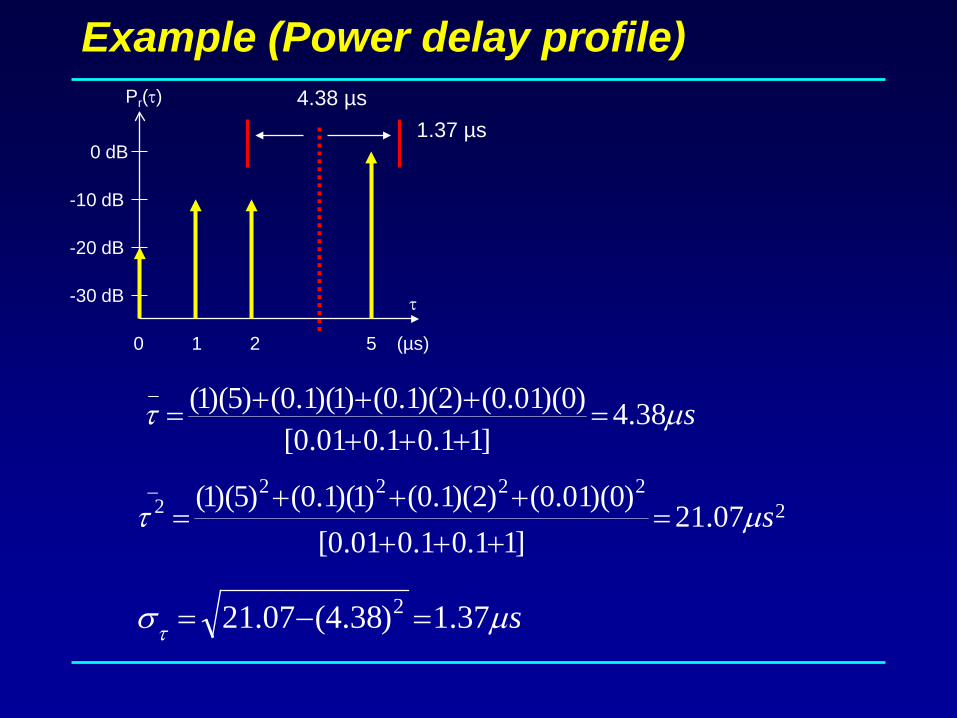
Example (Power delay profile)

-30 dB

-20 dB

-10 dB

0 dB

0 1 2 5

Pr(τ)

(µs)

τ

=++++++= sµτ 38.4

]11.01.001.0[)0)(01.0()2)(1.0()1)(1.0()5)(1(_

=+++

+++= 2

2222_2 07.21

]11.01.001.0[)0)(01.0()2)(1.0()1)(1.0()5)(1(

sµτ

=−= sµστ 37.1)38.4(07.21 2

1.37 µs4.38 µs

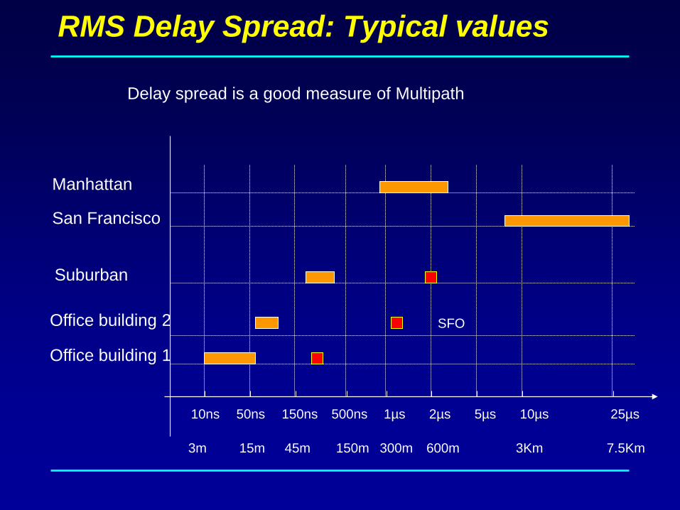
RMS Delay Spread: Typical values

10ns 50ns 150ns 1µs 2µs 5µs 10µs 25µs500ns

Office building 1

San Francisco

Manhattan

Suburban

Office building 2 SFO

Delay spread is a good measure of Multipath

3m 15m 45m 150m 300m 600m 3Km 7.5Km

Inter Symbol Interference

-30 dB

-20 dB

-10 dB

0 dB

0 1 2 5

Pr(τ)

(µs)

τ

1.37 µs4.38 µs

0 1 2 5 (µs)

Symbol time

4.38

στ

Symbol time > 10* στ --- No equalization required

Symbol time < 10* στ --- Equalization will be required to deal with ISI

In the above example, symbol time should be more than 14µs to avoid ISI.This means that link speed must be less than 70Kbps (approx)

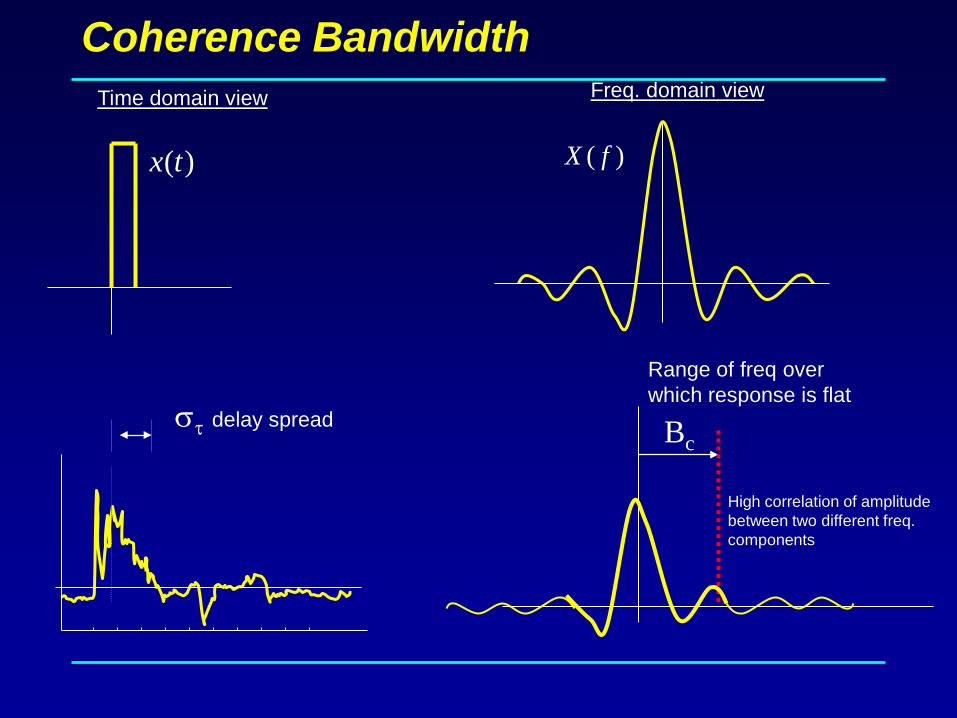
Coherence Bandwidth

)(tx

Time domain view

High correlation of amplitudebetween two different freq.components

Range of freq overwhich response is flat

Bcστ delay spread

)( fX

Freq. domain view

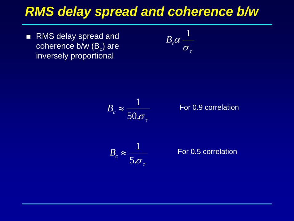
RMS delay spread and coherence b/w

RMS delay spread and coherence b/w (Bc) are inversely proportional

τσα 1

cB

τσ.501

≈cB For 0.9 correlation

τσ.51

≈cB For 0.5 correlation

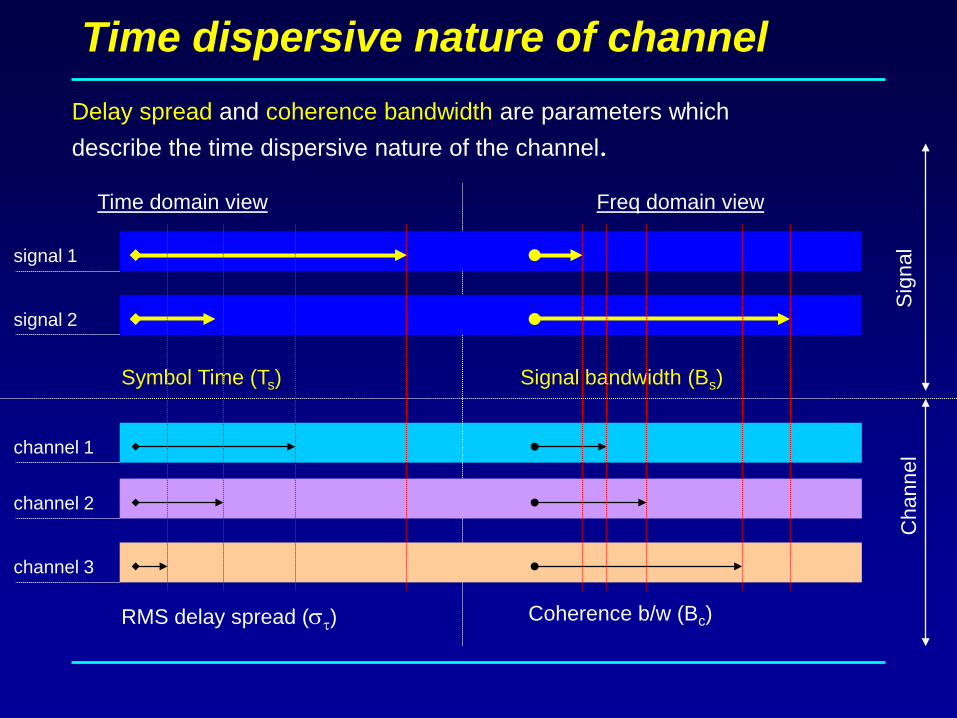
Time dispersive nature of channel

RMS delay spread (στ) Coherence b/w (Bc)

Time domain view Freq domain view

Delay spread and coherence bandwidth are parameters whichdescribe the time dispersive nature of the channel.

channel 1

channel 2

channel 3

Sig

nal

Cha

nnel

Symbol Time (Ts) Signal bandwidth (Bs)

signal 1

signal 2

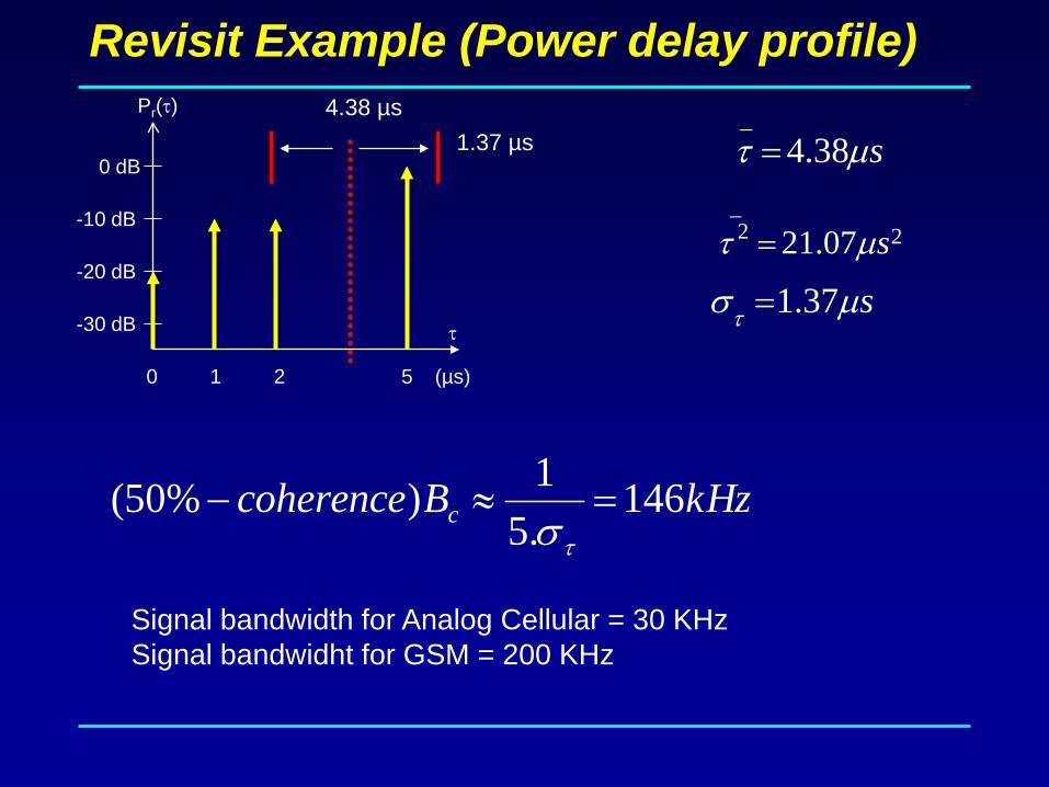
Revisit Example (Power delay profile)

-30 dB

-20 dB

-10 dB

0 dB

0 1 2 5

Pr(τ)

(µs)

τ

= sµτ 38.4_

= 2_2 07.21 sµτ

= sµστ 37.1

1.37 µs4.38 µs

kHzBcoherence c 146.51)%50( =≈−

τσ

Signal bandwidth for Analog Cellular = 30 KHzSignal bandwidht for GSM = 200 KHz

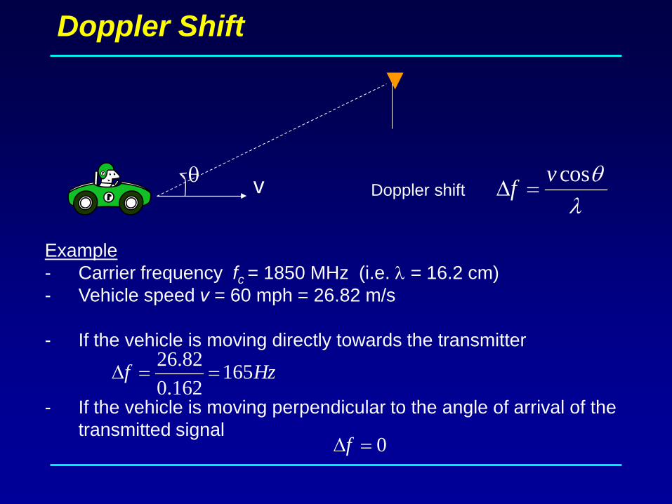
Doppler Shift

λθcosvf =∆vθ

Doppler shift

Example- Carrier frequency fc = 1850 MHz (i.e. λ = 16.2 cm)- Vehicle speed v = 60 mph = 26.82 m/s

- If the vehicle is moving directly towards the transmitter

- If the vehicle is moving perpendicular to the angle of arrival of the transmitted signal

Hzf 165162.0

82.26==∆

0=∆f

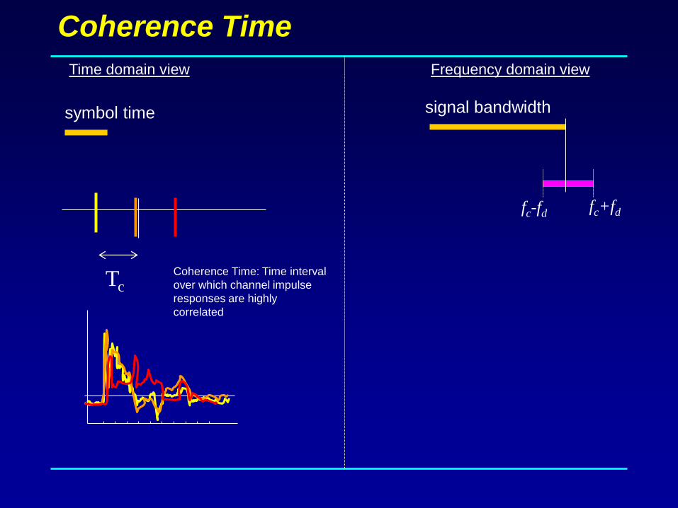
Coherence TimeTime domain view Frequency domain view

Coherence Time: Time intervalover which channel impulse responses are highly correlated

Tc

signal bandwidthsymbol time

fc+fdfc-fd

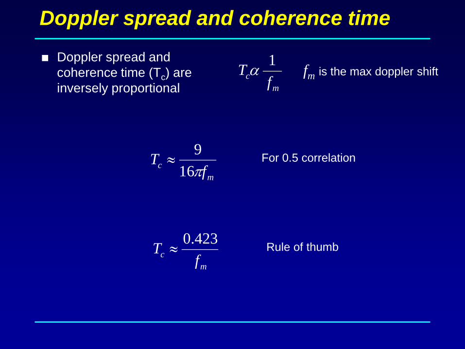
Doppler spread and coherence time

Doppler spread and coherence time (Tc) are inversely proportional m

c fT 1α

mc f

T 423.0≈ Rule of thumb

mc f

Tπ169

≈ For 0.5 correlation

fm is the max doppler shift

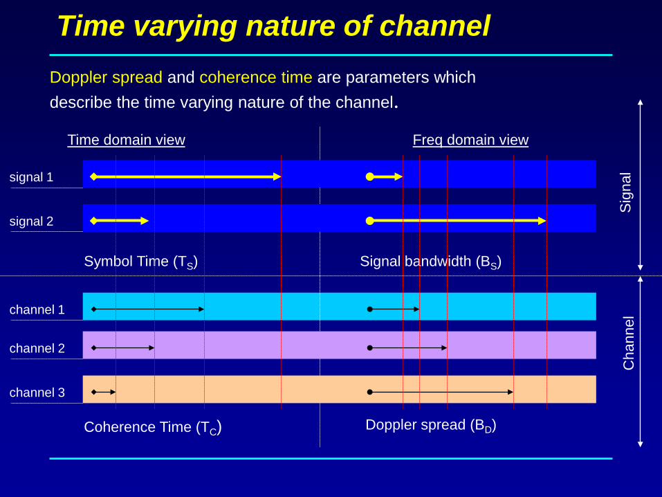
Time varying nature of channel

Coherence Time (TC) Doppler spread (BD)

Symbol Time (TS) Signal bandwidth (BS)

Time domain view Freq domain view

Doppler spread and coherence time are parameters whichdescribe the time varying nature of the channel.

channel 1

channel 2

channel 3

Sig

nal

Cha

nnel

signal 1

signal 2

Small scale fading

Multi path time delay

Doppler spread

Flat fading BC

BS

Frequency selective fading BC

BS

TC

TSSlow fading

Fast fading TC

TS

fading

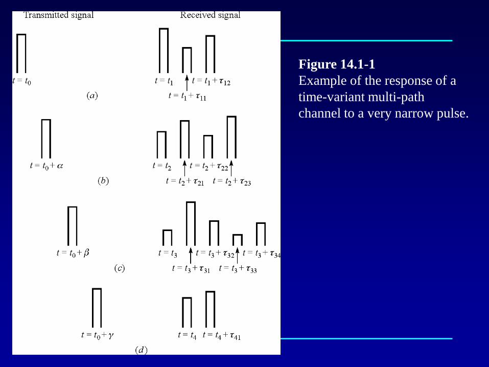
Figure 14.1-1Example of the response of atime-variant multi-pathchannel to a very narrow pulse.

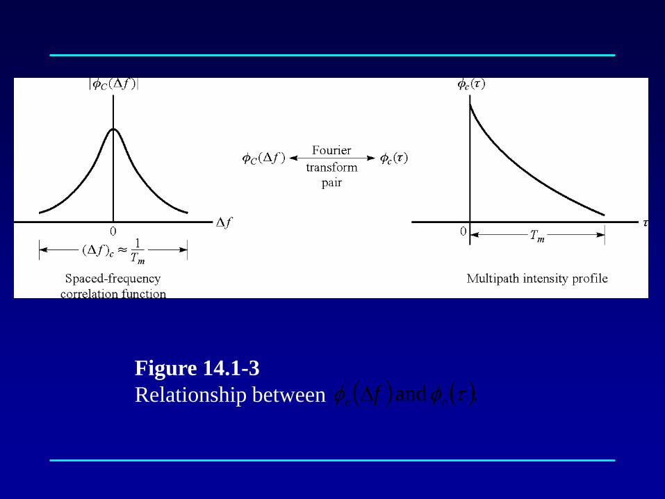
Figure 14.1-3Relationship between ( ) ( ). and τφφ cc f∆

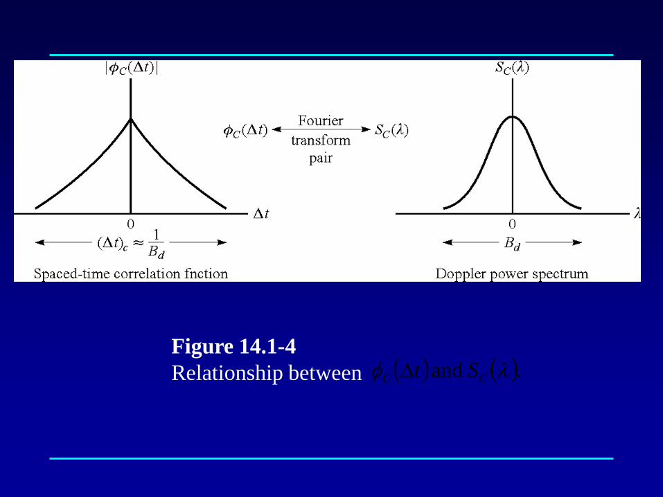
Figure 14.1-4Relationship between ( ) ( ). and λφ CC St∆

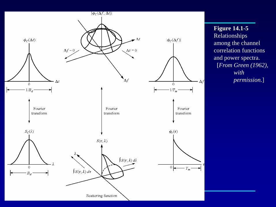
Figure 14.1-5Relationshipsamong the channelcorrelation functionsand power spectra.[From Green (1962),

withpermission.]

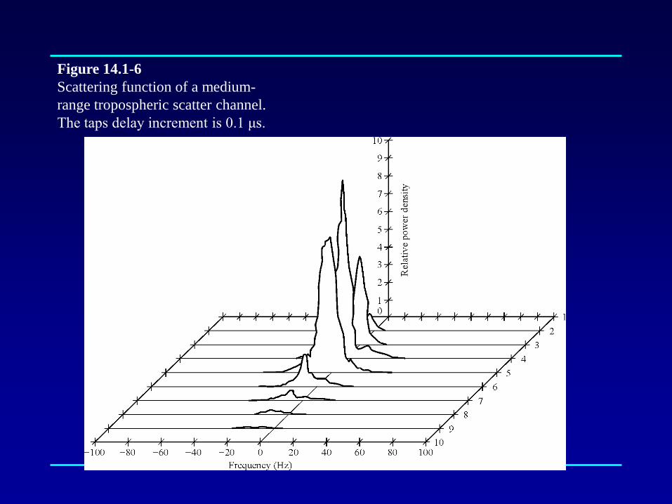
Figure 14.1-6Scattering function of a medium-range tropospheric scatter channel.The taps delay increment is 0.1 μs.

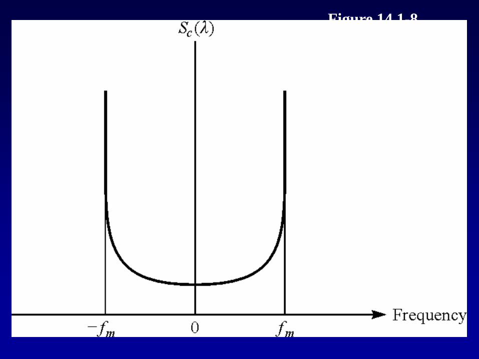
Figure 14.1-8Model of Dopplerspectrum for a mobile radio channel.

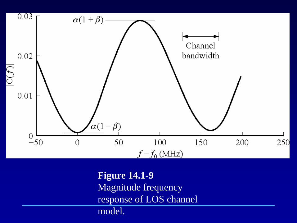
Figure 14.1-9Magnitude frequencyresponse of LOS channelmodel.

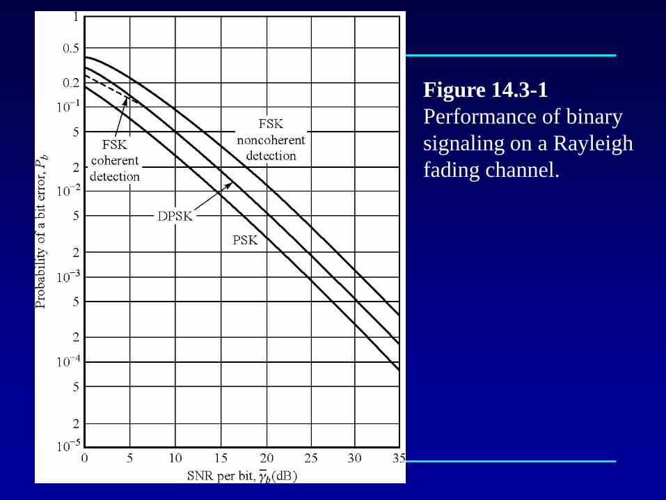
Figure 14.3-1Performance of binarysignaling on a Rayleighfading channel.