MPRAMunich Personal RePEc Archive

On the J-test for nonnested hypothesesand Bayesian extension

Surekha Rao and Moheb Ghali and John Krieg

Indiana University Northwest, Western Washington University

January 2008

Online at http://mpra.ub.uni-muenchen.de/14637/MPRA Paper No. 14637, posted 14. April 2009 00:38 UTC

On the J-test for the Non-nested Hypotheses and a Bayesian Extension

Moheb Ghali

John M. Krieg

Western Washington University

Bellingham, WA

K. Surekha Rao

Indiana University Northwest

Gary, IN 46408

Key Words: specification testing, non-nested hypotheses, Bayes factor, Bayesian Information

Criteria, Marginal likelihood

JEL Classification: C52, C11, C12

2

Abstract

Davidson and MacKinnon’s J-test was developed to test non-nested model specification. In

empirical applications, however, when the alternate specifications fit the data well the J test may

fail to distinguish between the true and false models: the J test will either reject, or fail to reject

both specifications. In such cases we show that it is possible to use the information generated in

the process of applying the J-test to implement a Bayesian approach that provides an unequivocal

and acceptable solution. Jeffreys’ Bayes factors offer ways of obtaining the posterior

probabilities of the competing models and relative ranking of the competing hypotheses. We

further show that by using approximations of Schwarz Information Criterion and Bayesian

Information Criterion we can use the classical estimates of the log of the maximum likelihood

which are available from the estimation procedures used to implement the J test to obtain

Bayesian posterior odds and posterior probabilities of the competing nested and non- nested

specifications without having to specify prior distributions and going through the rigorous

Bayesian computations.

3

I. INTRODUCTION

One of the most widely used tests for comparing non-nested hypotheses is the J test proposed by

Davidson and MacKinnon (1981). The non-nested tests of hypotheses arise in situations when

the alternate hypothesis cannot be derived as a special case of the null hypothesis. This may arise

either due to completely different sets of regressors in competing model specifications or

different distributions of the stochastic terms. This test appears in standard econometrics’

textbooks [e.g. Greene, 2003, and Davidson and MacKinnon, 2004], the Handbook of

Econometrics [Vol. 4, 1994], is included in the literature of standard econometrics programs [e.g.

EViews 5, and Shazam], and is the most commonly used non-nested test procedure (McAleer’s

(1995)).

When each of the competing hypotheses is successful in explaining the variations in the data, the

J-test may not be able to discriminate between alternative specifications. Some of the situations

in which the J test does not discriminate between the competing specifications have already been

noted. Godfrey and Pesaran (1982) state the following one or more conditions where the J test is

likely to over reject the true hypothesis: (i) a poor fit of the true model; (ii) low or moderate

correlation between the regressors of the two models; and (iii) the false model includes more

regressors than the correct specification. Davidson and MacKinnon (2004) agree that the J test

will over-reject, “often quite severely” in finite samples when the sample size is small or where

conditions (i) or (iii) above are obtained. Gourieroux and Monfort (1994) conclude that the test

is very sensitive to the relative number of regressors in the two hypotheses; in particular, the

power of the J test is poor when the number of regressors in the null hypothesis is smaller than

the number of regressors in the alternative one.

It is possible, however, to find examples in the literature where none of the above noted

conditions are violated1 and where the J test rejects all models.

2

1 That is to say that each of the alternative hypotheses fit the data extremely well, where the regressors of the alternative

hypotheses are correlated, where the alternatives have the same numbers of regressors, J-test is inconclusive.

2 McAleer’s (1995) survey of the use of non-nested tests in applied econometric work reports that out of 120 applications all

models were rejected in 43 applications. However, he did not break down the rejections by the type of test used.

4

Here, we give three examples of empirical work on the consumption functions that illustrates this

situation.

In the econometrics software EViews 5, the J test is used to compare two hypotheses regarding

the determinants of consumption. The first hypothesis is that consumption is a function of GDP

and lagged GDP. The alternative expresses consumption as a function of GDP and lagged

consumption. The data used are quarterly observations, 1947:2 – 1994:4. The conclusion reads:

“we reject both specifications, against the alternatives, suggesting that another model for the data

is needed.” [p. 581]. This conclusion is surprising, for the coefficient of determination reported

for each of the models was .999833, a value that would have lead most researchers to accept

either of the models as providing full explanation for the quarterly variability of consumption

over almost half a century.

Greene [2003] reported the results of comparing the same two consumption function hypotheses

using quarterly data for the period 1950:2 – 2000:4. The results of the test lead him to a similar

conclusion: “Thus, Ho should be rejected in favor of H1. But reversing the roles of Ho and H1…

H1 is rejected as well.” Although Greene did not report on the goodness of fit, it is very likely,

as in the EViews 5 data, that each of the models had explained almost all of the variation in

consumption.

The third example is found in Davidson and MacKinnon [1981] where they report on the results

of applying the J test to the five alternative consumption function models examined by Pesaran

and Deaton [1978]. In spite of the fact that the coefficients of determination for all the models

are quite high, ranging from .997933 to .998756 [Pesaran and Deaton, 1978, 689-91], each of the

models is rejected against one or more of the alternatives.

In this paper we show that when we wish to test alternative non-nested specifications that are

successful in explaining the observed variations, the J test is likely to be inconclusive. While

advances and improvements on the J test such as the Fast Double Bootstrap procedure [Davidson

and MacKinnon, 2002] have been made and are reported to increase the power of the test, it

appears that in doing empirical work researchers still use the standard J test [see for examples:

5

Faff and Gray (2006) or Singh (2004)]. In the discussion below we use the original test as this

allows for clarity of exposition.

In section II we point out the theoretical reasons why the test may lack power in testing model

specifications that fit a given set of data well. We do this by expressing the test statistic in terms

of the correlation between the variables in the alternative specification.

In section III we illustrate the problems encountered in using the J test in empirical work by

applying the test to two alternative specifications designed to explain monthly output behavior in

24 industries.

In section IV, we present a testing paradigm for non-nested hypothesis that can be implemented

to supplement the J test when the J test proves inconclusive. We use log-likelihood values which

are obtained in the process of applying the J test to approximate Bayesian information criteria

and Bayes factors. This allows us to circumvent the complexities of the Bayesian approach:

specifying the prior distributions and computations of marginal likelihoods. This specification

testing method yields results that do not depend on the choice of the null or the maintained

hypothesis. We illustrate the use of the Bayes factors in specification testing by applying it to the

same data on the 24 industries studied in section III.

II. THE J TEST

An “artificial regression” approach for testing non-nested models was proposed by Davidson and

MacKinnon [1981, 1993]. Consider two non-nested hypotheses that are offered as alternative

explanations for Y:

(2.1) H0: 1XY , and

(2.2) H1: 2ZY ,

Both disturbances satisfy the classical normal model assumptions, X has k1 and Z has k2

independent non-stochastic regressors.

6

We write the artificial compound model as:

(2.3) ZX)1(Y

If this model is estimated, we test the non-nested model by testing one parameter: when = 0,

the compound model collapses to equation (2.1) and when = 1, the compound model collapses

to equation (2.2).

Because the parameters of this model are not identifiable, Davidson and MacKinnon suggest

replacing the compound model (2.3) by one “in which the unknown parameters of the model not

being tested are replaced by estimates of those parameters that would be consistent if the DGP

[data generating process] actually belonged to the model they are defined.” (Davidson and

MacKinnon, 1993, p. 382). Thus, to test equation (2.1), we replace in (2.3) by its estimate

obtained by regressing Y on Z. If we write ˆZYz , the equation to be estimated to test whether

= 0 is:

(2.3’) z1 YX)1(Y .

Similarly, to test equation (2.2) we estimate by fitting equation (2.1) to the data and replace

X in (2.3) by X , or xY . The equation to be estimated to test (2.2) is then,

(2.3”) ZY)1(Y x .

The Davidson and MacKinnon J-test applies the t-test for the estimated coefficients on zY in

equation (2.3’) and xY in equation (2.3’’). A statistically significant t-statistic on the coefficient

of zY rejects H0 as the appropriate model and a significant t-statistic on the xY coefficient

results in the rejection of H1. For instance, in the consumption functions described in the

introduction, both t-statistics result in the rejection of each model. As some of the regressors in

(2.3’) and (2.3”) are stochastic, the t-test is not strictly valid. Davidson and MacKinnon (1993,

7

pp. 384-5) show as to why the J and P tests (which in [linear models] are identical) are

asymptotically valid.3

In this section we show that the t-test statistic for the significance of

in (2.3’), thus the

decision we make regarding the hypothesis (2.1), depends on the goodness of fit of the

regression of Y on Z, the goodness of fit of the regression (2.3’) as well as the correlation

between the two sets of regressors in (2.3’). We show this using the F ratio for testing = 0,

which is identical to the square of the t-value since we are interested in the contribution of only

one regressor zY . A similar statement applies to the test of the significance of (1 - ) in (2.3”).

Consider the OLS estimator of the coefficient of the model (2.3’). Using a theorem due to

Lovell (1963, p. 1001)4, the OLS estimate of and the estimated residuals will be the same as

those obtained from regressing the residuals of the regression of Y on X, YM x , on the residuals

of regressing zY on X, , zxYM ˆ ::

(2.4) xzxx MYMYM ˆ

Where, ]X)XX(XI[M 1x

, and ˆZYz and is the estimated regression coefficients of

Y on Z:

Writing, Z)ZZ(ZP 1z

, we write (2.4) as:

xzxx MYPMYM .

The OLS estimator of is then:

(2.5) YMPY]YPMPY[ˆxz

1zxz

3 They also add, “also indicates why they (J and P tests) may not be well behaved in finite samples. When the sample size is

small or Z contains many regressors that are not in S(X)…” We do not consider these situtions in what follows. 4 Lovell’s theorem 4.1 generalizes (to deal with seasonal adjustment) a theorem that was developed by R. Frisch and F. Waugh

for dealing with detrending data. Green (2003) extends the application to any partitioned set of regressors.

8

The residuals of OLS estimation of (2.4) are:

]YPMˆYM[ˆM zxxx

Since (2.4) has only one regressor, under the null hypothesis that = 0 the F-statistic is the

square of the t-statistic.

The sum of squares due to regression of equation (2.4), Q, is given by:

(2.6) ˆDˆQ , where zxz YMYD

Consider regressing Y on X only and denote the residuals of that regression by YMu x and

regressing zY on X and denote the residuals of that regression by: zx YMˆ . We can then write:

(2.5’) uˆ)ˆˆ(ˆ 1 , and

(2.6’) 221xz

1zxzzx

ˆ)ˆu(ˆu)ˆˆ(ˆuYMY]YMY[YMYQ

The residuals from OLS estimation of (2.4) can be written as:

ˆ)uˆ()ˆˆ(uˆˆu]YPMˆYM[ˆM 1zxxx

The sum of the squared residuals from estimating (2.4) is:

(2.7) ]ˆ/)ˆu[(uˆMˆ 222x

This sum of squares has (T–k1–1) degrees of freedom, where T is the number of observations

and k1 is the number of variables in X.

9

Thus, under the hypothesis that = 0, the F-statistic is5:

(2.9) )1kT,1(F 1 /[Q ˆMˆx / (T-k1-1)] = )1kT(

)ˆu(ˆu

)ˆu(1222

2

This test statistic can be expressed in terms of correlations between the variables. We show in the

Appendix that:

(2.10) 2

yyyxyz2xy

2yx

2

yyyxyz1

12

]RRR[)R1)(R1(

]RRR)[1kT()1kT,1(F

zx

zx

Where we placed the superscript 2 to denote that it is a test for the second model, equation (2.2),

under the assumption that the first model is true, and where:

2yxR is the coefficient of determination of the regression of Y on X only,

2

yzR is the coefficient of determination of the regression of Y on Z only,

2xyR is the coefficient of determination of the regression of zY on X,

zx yyR is the correlation coefficient of xY and zY , and since these are linear combinations of X

and Z respectively, zxyyR is the canonical correlation of the alternative regressors X and Z.

6

Because the J test is symmetric, the second part of the J test, maintaining (2.2) and testing for the

significance of (1 - ) in (2.3”), the test statistic, denoted as F1 is:

(2.11) 2

yyyzyx2zy

2yz

2

yyyzyx2

21

]RRR[)R1)(R1(

]RRR)[1kT()1kT,1(F

zx

zx

5 See equation (22) of Godfrey and Peseran (1983).

6 Where there is only one regressor in each of X and Z, the coefficientzx yy

R is the correlation between the two regressors and

the test statistic simplifies to:

xzyxyz2yz

2yx

2xz

2xzyxyz1

12

RRR2RRR1

]RRR)[1kT()1kT,1(F

.

10

From these two test statistics we note the following:

a) When sample size is small, the difference between the numbers of regressors in

the competing model will affect the sizes of the test statistics. If the data were

generated by the model of (2.1), the test statistic F1 will get smaller as the

number of regressors in the alternative model, k2, increases. This may lead to the

rejection of (2.1) in favor of the alternative model (2.2), particularly if the number

of regressors k1 is small. This is consistent with Godfrey and Pesaran’s (1982)

simulation-based findings as well as with Gourieroux and Monfort (1994) who

conclude that the test “is very sensitive to the relative number of regressors in the

two hypotheses; in particular the power of the J test is poor when the number of

regressors in the null hypothesis is smaller than the number of regressors in the

alternative one.” However, the influence of the differentials in the number of

regressors will become negligible as sample size increases.

b) When a model is successful in explaining the variations in Y the J test is likely to

reject it. To see this clearly, assume that the alternative regressors are orthogonal

so that 0Rzx yy . If model (2.1) is successful, the high coefficient of

determination 2

yxR will increase the numerator of (2.11) while reducing the

denominator, thus increasing the value of the test statistic F1 which leads to

rejection of the model (2.1). Similarly, if the model (2.2) is successful in

explaining the variations in Y, the high value of 2

yzR will increase the value of the

test statistic F2 which leads to the rejection of model (2.2). When both models

are successful in explaining the variations in Y, the combined effect of high

2

yxR and 2yzR leads us to reject both models. Such was the situation in Davidson

and MacKinnon [1981] report on the five alternative consumption function where

the coefficients of determination for all the models ranged from .997933 to

.998756, yet all the models were rejected. This would be at variance with the

conclusion reached by Godfrey and Pesaran (1983) “when sample sizes are small

the application of the (unadjusted) Cox test or the J-test to non-nested linear

regression models is most likely to result in over rejection of the null hypothesis,

11

even when it happens to be true, if …the true model fits poorly”, unless the fit of

the false model also fits poorly.

c) zx yy

R is the canonical correlation coefficient of the sets of regressors X and Z.

Higher values of this correlation would reduce the numerator and increase the

denominator of both (2.10) and (2.11), lowering the values of the F statistics. The

effect would reduce the likelihood of rejecting either of the competing

hypotheses. The reverse, as stated in Godfrey and Pesaran (1983) is also true:

“when the correlation among the regressors of the two models is weak” the J test

“is most likely to result in over rejection of the null hypothesis, even when it

happens to be true,”

The effect of the coefficients of determination of the alternative model specifications on the F

statistic is shown in Figure 1.7 In this figure, the light grey areas represent combinations of 2

yxR

and 2

yzR that result in rejecting the X model (2.1) and failing to reject the Z model (2.2). This is

appropriate since for those combinations, the model using the set of explanatory variables Z is

clearly superior to that which uses the set X. The dark grey areas represent combinations that

result in rejecting the model that uses the set of explanatory variables Z and failing to reject the

model which uses X. Again, this is clearly appropriate. The interior white areas represent

combinations of the coefficients of determination for which the J test fails to reject both models.

Within those areas comparisons of the coefficients of determination for the two alternative

models, particularly for large samples would have led to the conclusion that neither model is

7 The coefficients of determination and the canonical correlations are subject to restrictions. Since the quadratic form

]ˆ/)ˆu[(uˆMˆ 222x is positive semi-definite, 222 )vu(vu

, that is:

2

yyyxyz2xy

2yx ]R.RR[)R1)(R1(

zx . The restrictions imply that when the canonical correlation between X and

Z is zero (the two sets of alternative explanatory variables are orthogonal), 1RR 2

yz

2

yx . Thus, in figures (1.a), (1.b) and

(1.c) where the canonical correlation is set at zero, the only feasible region is the triangle below the line connecting the points

1R 2

yx and 1R 2

yz . When the canonical correlation is different from zero, the restriction on the relationship between the

coefficients of determination result in the elliptical shape of the feasible region shown in the second and third columns of Figure

1. Combinations of the coefficients of determinations outside of the ellipse violate the restriction.

12

particularly useful in explaining Y. The black areas represent combinations of 2

yxR and 2

yzR that

result in rejecting both hypotheses. What is remarkable is the size of these areas compared to the

other areas and the fact that the black area encompasses combinations of 2

yxR and 2

yzR that,

because of their large difference, would reasonably preclude a researcher from employing the J

test.8 For instance, consider two competing models in the middle panel (the case of n = 100 and

4.R 2

xz ). If one model had 9.R2

yx and the other 6.R2

yz , the J test would reject both

models despite the fact that the X model would be traditionally viewed as the superior model

based solely on the comparisons of the coefficients of determination.

The canonical correlation of the competing model’s independent variables impacts the

permissible values of the J test. The first panel demonstrates a canonical correlation between

regressors set at zero, in the second panel it is set at .40 and in the third it is set at .90. It is worth

noting that when the canonical correlation is greater than zero, the size of the permissible region

decreases as the correlation increases. In the extreme case where the canonical correlation

approaches 1, so that each of the variables X and Z are a linear combination of the other, the

permissible combinations of the coefficients of determination, R2

xy and R2

yz will lie on the 45

degree diagonal emanating from the origin.

The effect of sample size on both the permissible region, we present the figures for sample sizes

30, 100 and 1000 in each of the three panels. The size of the permissible region depends only on

the value of the canonical correlation, and is independent of sample size as would be expected.

It is clear from these figures that as sample size increases, the area in which the J test would lead

to the rejection of both hypotheses expands and thus covers increasingly larger areas of the

permissible region.

8 The white spaces outside of the shaded areas are regions where the combinations of the coefficients of determination that are

not permissible- they result in violating the requirement that 222x

ˆ/)ˆu[(uˆMˆ ] is positive semi-definite.

Figure 1: J-Test Results for Various N, 2

xzR , 2

xyR , and 2

yzR

0R 2

xz 40.R 2xz 90.R 2

xz

n =

30

n =

100

n =

1000

Notes: Black area represents reject both region, red (light grey) area represents reject the X model and fail to reject the Z model, blue

(dark grey) represents reject the Z and fail to reject the X model, interior white areas represents fail to reject both models. All graphs were

produced at a 5% level of significance.

III. DETERMINANTS OF MONTHLY VARIATIONS IN INDUSTRY OUTPUT

3.1 Alternative Model Specifications for Production Behavior

We now apply the J test to compare two model specifications that have been used to explain

monthly variations in industry output (Ghali, 2004). In both specifications monthly output is

determined by sales. In one specification the stock of inventories also influences production,

while in the other specification inventory stock does not play a role. The two specifications also

differ in the way in which the sales variable enter into the specification.

Minimizing the discounted cost over an infinite horizon for the traditional cost function used by

many researchers results in the Euler equation reported by Ramey and West (1999, p. 885).

Solving for current period output, Qt and assuming the cost shocks to be random,9 we get the

following equations:

(3.1) ii41i31i22i

2

1ii10i uHSQ]QbQb2Q[Q

where Qi is output in month “i”, Si is sales and Hi is the inventory stock at the end of the month.

The minimization of the cost using an alternative cost function (Ghali, 1987) and solving the

resulting Euler equation for output we get:

(3.2) tiQ = itt2it10 uSS ,

where Sit represents sales in month “i” of production planning horizon “t” and tS is the average

sales over the production planning horizon.

We apply the J-test to the two specifications M1 in equation (3.1) and M2 in equations (3.2). as

specifications are non-nested hypotheses explaining the monthly variability of production.

9 The empirical justification for this assumption is that the estimates reported in the literature for the effect of factor price

variations on cost are not strongly supportive of the assumption that the cost shocks are observable. Ramey and West (1999)

tabulated the results of seven studies regarding the significance of the estimated coefficients for input prices. They reported that

wages had a significant coefficient in only one study and material prices in one study. (Ramey and West, 1999, 907). More

detailed discussion is given in Ghali (2004).

15

3.2 The Data

The data we use are those used by Krane and Braun (1991).10

These data are in physical

quantities, thus obviating the need to convert value data to quantity data and eliminating the

numerous sources of error involved in such calculations11

. The data are monthly, eliminating

the potential biases that may result from temporal aggregation.12

They are at the four-digit SIC

level or higher, reducing the potential biases that may result from the aggregation of

heterogeneous industries into the two-digit SIC level.13

The data are not seasonally adjusted,

thus obviating the need for re-introducing seasonals in an adjusted series.14

A description of the

data and their sources is available in Table 1 of Krane and Braun (1991, 564-565). We use the

data on the 24 industries studied by Ghali (2005).

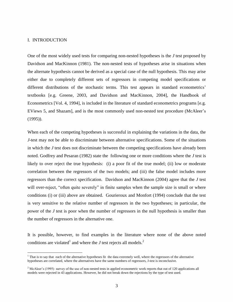
3.3 Empirical Results15

In Table 1 the results of applying the J test to compare the two specifications are reported. In the

first set of columns we report the results of testing M1, equation (3.1) assuming that M2,

equation (3.2) is maintained. This is done by estimating the parameters of equation (3.2) using

OLS as suggested by Davidson and MacKinnon,16

The coefficient of determination, R2, of those

regressions are reported in the first column, We then used the predicted values of Qi from that

regression as an added regressor in the estimation of equation (1’). The coefficient of the added

regressor, iQ , is reported in the second column and its t value in the third column. If the

coefficient of the added regressor is significantly different from zero, the model specification

(3.1) is rejected in favor of the model specification (3.2). As the fourth column shows, this was

the case for all of the industries.

The process is reversed in the second set of columns of Table 1. We now maintain the model

specification of equation (3.1) and test that of equation (3.2). The last column of this set of

10 We are very grateful to Spencer D. Krane who made this data available. 11 For discussion of the potential measurement errors in converting value to quantity data for inventory stocks,see Krane and

Braun (1991, 560 –562). 12 See Ghali (1987) and Lai (1991). 13 For discussion of the potential biases see Krane and Braun (1990, 7). 14 For example see Ramey (1991). She had to re-introduce seasonality as the data she was using was seasonally adjusted. 15 The results reported in Table (1) are from Ghali 2007 reproduced with permission from publisher. 16 All equations were estimated under the assumption of an AR(1) process for the error term.

16

columns shows that the model of equation (3.2) is rejected in favor of the model specification of

equation (3.1).

As can be seen from Table 1, for all industries studied both competing specifications are rejected

by the J-test. “When both models are rejected, we must conclude that neither model is

satisfactory, a result that may not be welcome but that will perhaps spur us to develop better

models.”(Davidson and MacKinnon, 1993, p. 383). However, it should be noted that each of the

model specifications explains very high proportion of the monthly variation of output that as seen

by the high coefficients of determination reported for each. It may be that because each of the

specifications is so successful in explaining the behavior of output, the J test is not able to

distinguish between them. In other words, if the maintained specification is successful in

explaining the dependant variable, the correlation between the predicted value and the dependant

value will be significant, and so will be the coefficient of the predicted value when added as a

regressor in the artificial compound model.

17

TABLE 1: DAVIDSON- MACKINNON J TEST INDUSTRY SAMPL

E

PERIOD

H2Maintained, H1Tested H1Maintained H2 Tested

R22

t H1 R12

t H2

Asphalt1 1977:01-

1988:12 .955 .767 16.76 R .980 .959 14.98 R

Bituminous

Coal

1977:01-

1988:09 .606 .371 8.432 R. .944 .958 34.276 R

Cotton Fabric 1975:01-

1986:12 .936 .507 13.201 R. .944 .578 14.242 R

Distillate Fuel 1977:01-

1988:12 .686 .330 7.000 R .943 1.060 28.310 R

Gasoline 1977:01-

1988:12 .733 .246 3.750 R .904 1.058 19.085 R

Glass

Containers

1977:01-

1989:03 .670 .231 4.301 R .902 .969 20.822 R

Iron and Steel

Scrap

1956:01-

1988:12 .969 .596 15.868 R .966 .642 18.185 R

Iron Ore 1961:01-

1988:12 .873 .376 12.489 R .966 1.087 37.225 R

Jet Fuel 1977:01-

1988:12 .899 .182 3.932 R .983 .961 28.234 R

Kerosene 1977:01-

1989:03 .823 .318 5.551 R .949 1.155 26.824 R

Liquefied Gas 1977:01-

1988:12 .376 .441 7.015 R .917 1.045 31.742 R

Lubricants 1977:01-

1988:12 .496 .198 2.940 R .912 1.046 25.697 R

Man-made

Fabric

1975:01-

1986:12 .904 .587 11.894 R .903 .553 10.606 R

Newsprint

Canada

1961:01

1988:12 .838 .243 8.769 R .966 .965 44.514 R

Newsprint US 1961:01-

1988:12 .991 .402 12.963 R .996 .773 30.423 R

Petroleum

Coke

1977:01

1989:03 .933 .216 5.377 R .983 .847 20.469 R

Pig Iron 1961:01-

1988:12 .997 .924 39.214 R .985 .242 8.294 R

Pneumatic

Casings

1966:01-

1988:12 .802 .317 12.310 R .956 .983 40.722 R

Residual Fuel 1977:01-

1988:12 .965 .313 6.950 R .991 .997 29.659 R

Slab Zinc 1977:01-

1988:03 .888 .254 5.283 R .976 1.065 28.974 R

Sulfur 1961:01-

1988:12 .889 .281 6.348 R .988 1.024 72.875 R

Super

Phosphates

1981:01-

1988:12 .941 .325 6.743 R .981 .936 21.897 R

Synthetic

Rubber

1961:01

1984:12 .833 .198 5.567 R .965 1.026 34.948 R

Waste Paper 1977:01

1988:02 .874 .440 6.253 R .962 .896 19.073 R

18

IV. A BAYESIAN SOLUTION

In many non-standard testing of hypotheses situations when the classical procedures lead to

inconsistent results as in the case of J-test, the Bayesian approach provides an alternative that is

consistent (see, for example; Zellner (1971, 1994), Berger and Pericchi (2001)). The Bayesian

paradigm is generally more involved as it necessitates the specification of prior distribution for

the parameters as well as the hypotheses, obtaining marginal likelihoods, Bayesian posterior

odds and Bayes factors for the competing hypotheses. Therefore, it is not surprising that we find

a rather limited number of applications of the Bayesian approach even though it is intuitively

more appealing and provides consistent and meaningful results.

Schwarz (1978) suggested approximations to Schwarz Information criterion (SIC) and Bayesian

Information criterion (BIC) using the log of the likelihood values. Later, Kass and Raftrey

(1995) provided extensions and applications for computing Bayes factors. By combining these

approaches we can use the maximum likelihood values obtained from the estimation needed for

the J test to approximate the Bayesian posterior odds and the Bayes factor.

We give below a brief overview of the Bayesian approach and then describe how the log of the

maximum likelihood can be used to asymptotically approximate the Bayes factor and to provide

consistent results for non nested model selection.

4.1 An overview of the Bayesian Hypothesis Testing for Nested and Non-nested hypotheses

The theory of Bayesian testing of hypotheses is built around the concept of posterior

probabilities of hypotheses and the Bayes factor, which were first introduced by Jeffreys (1935,

1961). Bayesian model comparison concepts and the issues that arise in empirical applications

have been discussed by Zellner (1971), Kass and Raftrey (1995), Berger and Pericchi (2001)

and Koop (2003), amongst many others. Schwarz (1978) paved the way for interplay between

the Information Criteria and the Bayes factor for Bayesian specification test. We use Schwarz’

approximation of Bayesian information criteria and the log likelihood values to calculate Bayes

factors for the competing models.

19

If M1, M2 are two different model specifications17

for a given data D, the posterior odds ratio

K12 is given by

(4.1) K12 = [P (Data/H1)/P (Data/H2)]* [P (H1) /P (H2)]

Or:

(4.2) Posterior Odds = Bayes factor X Prior odds

In the absence of any definitive information or if we have little information we treat the two

hypotheses a priori equally likely implying P(H1) = P(H2) = ½ , and the prior odds ratio

[P (H1) / P (H2)] is equal to 1. If prior odds equal one, from (4.2), the Posterior odds ratio is

same as the Bayes factor.

The Bayes factor is the ratio of the posterior probability of observing the data if Hi, i=1, 2 were

true. Bayes factor K12 measures the extent to which data supports Hypothesis l over Hypothesis

2 and the evidence against Hypothesis 2.

P(D/Hi, i=1,2…k) , the marginal likelihood and is also known as the weighted likelihood or the

predictive likelihood and is given by

(4.4) P (D/Hi) = i, Hi) π (i/ Hi) di i=1.2….,k

Where i, is the parameter under Hi and π (i/ Hi) di is its prior probability density and

i, Hi) is the probability density of D given the value of i under the hypothesis

Hi or the likelihood function of .

In the traditional Bayesian approach, we must specify the prior distribution π(i/ Hi) for the

parameter(s) i. The use of prior distribution is the double edged sword for the Bayesian

approach. This is what provides that extra information in applications and the advantage over

17 The two model specifications must be exahustive if we need to obtain Posterior probabilities of hypothesis from the posterior

odds. The results can be easily extended for k model specifications.

20

the classical approach. On the other hand, the specification of the prior is one of the most

controversial aspects of the Bayesian approach.

The quantity P(D/Hi), is the predictive probability of the data; that is the probability of seeing

this data which is calculated before the data is observed. Bayes factor which is the ratio of these

marginal probabilities of the data shows the evidence in favor of or against the hypothesis. In

case of two hypotheses, i=1,2:

(4.5) K12 = P (D/H1)/ P (D/H2)

(4.6) K12 = 1, H1) π (1/ H1) d1 / 2, H2) π (2/ H2)

d2

If K12 is greater than 1, the data favors Hypothesis 1 (Model M1) over Hypothesis 2(Model M2)

and if K12 is less than 1, the data favors Hypothesis 2 (model M2).

4.2 Bayes factor, BIC and the Likelihood values

Although Bayes factors are fairly versatile and universally applicable for specification testing,

calculation of marginal likelihoods is extremely demanding and sometimes these may not even

exist (Leamer 1978). There has been great interest in finding alternate methods and

approximations to Bayes factors. Various information criterions have been developed to this

effect, which are not very rigorous, yet they are approximations to quantities that are either

Bayesian or have a Bayesian justification. Akaike, Schwarz and Bayesian information criterion

are frequently used.

From Schwarz (1978) we note that the log of the Marginal likelihood can be approximated by the

log of the Likelihood minus a correction term. This asymptotic approximation to the marginal

likelihoods can be used to compute Bayes factor and can be applied to obtain the Posterior odds

21

and the posterior probabilities of the two competing models from the likelihood values for each

model (Koop 2003 and Kass and Raftrey 1995 ). This is how it works in practice:

(4.7) -2 SIC BIC

(4.8) SIC = (log[ pr( D 1/,,M1] – log[ pr( D/ , M2] ) – ½ (p1 - p2 ) log (n),

Where i-1,2 are the MLE under Model Mi, p1, and p2 are the number of parameters in

models 1 and 2 respectively and n is the sample size.

(4.9) BIC (M1) = 2 log pr (D/ /, M1] – p1 ln(n) ,

(4.10) BIC (M2) = 2log pr [ p( D/ 2 M2] – p2 ln(n) , and

(4.11) 2 log K12 = BIC (M2) – BIC (M1)

Since BICs can be calculated from likelihood values, we can calculate twice the Bayes factor

from (4.11) without specifying the prior distribution. Once we know the 2 log K12 and since

Models M1 and M2 are exhaustive in this case we can obtain posterior probabilities 1 and 2

for Models M1 and M2 by using the relationship:

(4.12) 1 = ; and 2 =

Although in all empirical applications we use only the posterior odds and the Bayes factors, we

can also use the posterior probabilities of individual specifications and hypothesis for ranking

and comparing different model specifications in case of larger number of alternate model

specifications. A decision to accept or reject a particular model generally requires choosing a

model that minimizes an appropriate loss function.

Jeffreys in (1961, appendix B) also proposed some rules of thumb for interpreting Bayes factor.

If we consider 0 < 2 Log(K21)<2 ; the evidence against M1 is not worth more than a bare

22

mention, if 2 < 2 Log(B21)< 6, the evidence against M1 is positive and if 6<2 Log(B21)<10, the

evidence against is strong and if 2 Log(B21)>10, the evidence against M1 is very strong. We

shall use these guiding rules to make decisions for choosing between two cost functions for all

twenty five industries in our data set.

4.3 Bayes Factors and the Model Specification:

Let us consider that the model specification M1 in equation 3.1 is the Null Hypothesis H0 and

the maintained hypothesis is model specification M2 in equation 3.2. Bayes factor K12 will

measure the evidence for Model 1 against model 2 and K21 will measure the evidence against

M1. These results are given in the Table 2 below. The results are quite consistent and

unequivocal that specification M2 in equation 3.2 is strongly supported by the data for 23 of the

25 industries ( except, iron scrap and pig iron) irrespective of the choice of the Null and the

maintained hypotheses.

23

Table 2: Bayes factors and Posterior Probabilities of Models M1 and M2

2 Log

K21

K21 Evidence

against M1

2 log

(K12)

K12 Evidence

Against M2 1 2

Asphalt 101.99 1.4E+22 very Strong -101.99 7.12E-23 Not worth

mention

7.12E-23 1

Beer 18.56 10695.36 very Strong -18.56 9.35E-05 Not worth

mention

9.35E-05 0.999907

Bituminous

Coal

322.56 1.1E+70 very Strong -322.56 9.06E-71 Not worth

mention

9.06E-71 1

Cotton

Fabric

25.09 280624.6 very Strong -25.09 3.56E-06 Not worth

mention

3.56E-06 0.999996

Distillate

Fuel

249.23 1.32E+54 very Strong -249.23 7.6E-55 Not worth

mention

7.6E-55 1

Gasoline 154.64 3.79E+33 very Strong -154.64 2.64E-34 Not worth

mention

2.64E-34 1

Glass

Containers

178.87 6.94E+38 very Strong -178.87 1.44E-39 Not worth

mention

1.44E-39 1

Iron Scrap -18.37 0.000103 not worth

mention

18.37 9739.505 Very strong 0.999897 0.000103

Iron Ore 353.21 4.99E+76 very Strong -353.21 2E-77 Not worth

mention

2E-77 1

Jet Fuel 257.77 9.43E+55 very Strong -257.77 1.06E-56 Not worth

mention

1.06E-56 1

Kerosene 175.58 1.34E+38 very Strong -175.58 7.47E-39 Not worth

mention

7.47E-39 1

Liquified

Gas

277.70 2E+60 very Strong -277.70 5E-61 Not worth

mention

5E-61 1

Lubricants 232.60 3.22E+50 very Strong -232.60 3.11E-51 Not worth

mention

3.11E-51 1

Man-made

Fabric

7.61 44.98217 Strong -7.61 0.022231 Not worth

mention

0.021748 0.978252

Newsprint

Canada

520.39 1E+113 very Strong -520.39 1E-113 Not worth

mention

1E-113 1

Newsprint

US ARD

513.09 2.6E+111 very Strong -513.09 3.8E-112 Not worth

mention

3.8E-112 1

Newsprint

US

276.53 1.12E+60 very Strong -276.53 8.97E-61 Not worth

mention

8.97E-61 1

Petroleum

Coke

125.52 1.81E+27 very Strong -125.52 5.53E-28 Not worth

mention

5.53E-28 1

Pig Iron -508.78 3.3E-111 not worth

mentioning

508.78 3E+110 Very strong 1 3.3E-111

Pneumatic

casings

512.75 2.2E+111 very Strong -512.75 4.5E-112 Not worth

mention

4.5E-112 1

Residual

Fuel

197.12 6.36E+42 very Strong -197.12 1.57E-43 Not worth

mention

1.57E-43 1

Slab Zinc 216.21 8.88E+46 very Strong -216.21 1.13E-47 Not worth

mention

1.13E-47 1

Sulphur 722.68 8.5E+156 very Strong -722.68 1.2E-157 Not worth

mention

1.2E-157 1

Super

Phosphate

148.91 2.17E+32 very Strong -148.91 4.62E-33 Not worth

mention

4.62E-33 1

Synthetic

Rubber

460.03 7.8E+99 very Strong -460.03 1.3E-100 Not worth

mention

1.3E-100 1

Waste Paper 180.21 1.36E+39 very Strong -180.21 7.37E-40 Not worth

mention

7.37E-40 1

24

IV. CONCLUSION

In earlier research the original J test has been shown to over reject when the true model fits the

data poorly, when the regressors in the models being compared are highly correlated, or when

the false model contains more regressors than the true model. We presented examples where the

alternative specifications fit the data well but the J test did not distinguish between them: the J

test either rejects, or fails to reject both specifications.

To supplement the J test when such situations arise we proposed a Bayesian approach that uses

the estimated maximum likelihood values obtained in the process of conducting the test.

Bayesian posterior odds allow us to overcome the problems associated with the J-test. Jeffreys’

Bayes factors offer ways of obtaining the posterior probabilities of the competing model

specifications and relative ranking of the competing specifications. We showed that by using

approximations of Schwarz Information Criterion and Bayesian Information Criterion we can

use the classical estimates of the log of the maximum likelihood to obtain Bayesian posterior

odds and posterior probabilities of the competing nested and non- nested models.

Bayesian testing for nested and non-nested specifications is currently an active area of research.

Bayes intrinsic factors and Bayes fractional intrinsic factors and default Bayes factors of Berger

and Pericchi (2001), the approximations by Gelfand and Dey (1994) and Chib (1995) are all

very promising for applications in complex economic models and in case of panel data models.

The method we proposed in this paper has an advantage as it gives us all the benefits of the

Bayesian paradigm and the Bayes factors without having to specify prior probabilities and going

through the extensive Bayesian computations.

25

APPENDIX

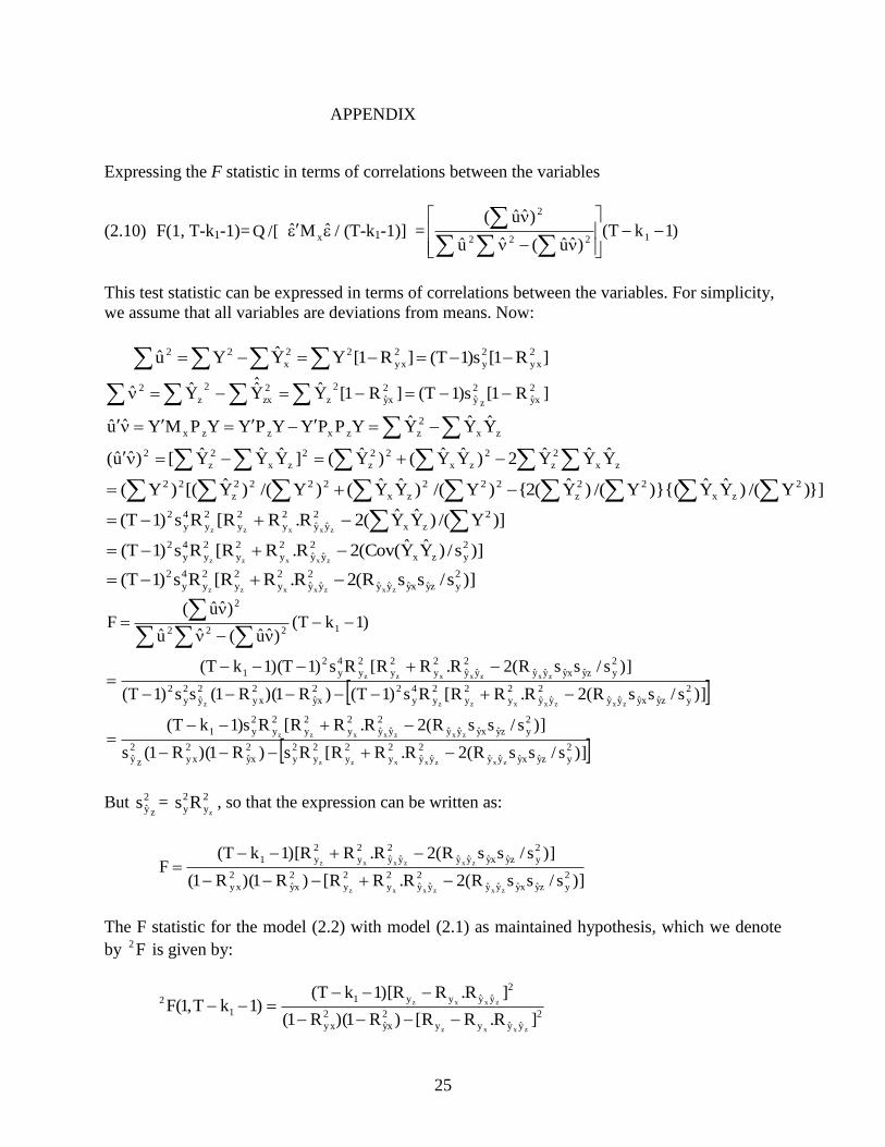
Expressing the F statistic in terms of correlations between the variables

(2.10) F(1, T-k1-1)= /[Q ˆMˆx / (T-k1-1)] = )1kT(

)ˆu(ˆu

)ˆu(1222

2

This test statistic can be expressed in terms of correlations between the variables. For simplicity,

we assume that all variables are deviations from means. Now:

]R1[s)1T(]R1[YYYu 2

yx

2

y

2

yx

22

x

22

]R1[s)1T(]R1[YYˆ

Yˆ 2

xyz

2

y

2

xy

2

z

2

zx

2

z

2

zx

2

z

2

zx

22

z

2

zx

2

z

2

zx

2

zzxzzx

YYY2)YY()Y(]YYY[)ˆu(

YYYYPPYYPYYPMYˆu

}])Y/()YY)}{(Y/()Y(2{)Y/()YY()Y/()Y([)Y( 2

zx

22

z

222

zx

2222

z

22

])Y/()YY(2R.RR[Rs)1T( 2

zx

2

yy

2

y

2

y

2

y

4

y

2

zxxzz

)]s/)YY(Cov(2R.RR[Rs)1T( 2

yzx

2

yy

2

y

2

y

2

y

4

y

2

zxxzz

)]s/ssR(2R.RR[Rs)1T( 2

yzyxyyy

2

yy

2

y

2

y

2

y

4

y

2

zxzxxzz

)]s/ssR(2R.RR[Rs)R1)(R1(s

)]s/ssR(2R.RR[Rs)1kT(

)]s/ssR(2R.RR[Rs)1T()R1)(R1(ss)1T(

)]s/ssR(2R.RR[Rs)1T)(1kT(

)1kT()ˆu(ˆu

)ˆu(F

2

yzyxyyy

2

yy

2

y

2

y

2

y

2

y

2

xy

2

y xz

2

y

2

yzyxyyy

2

yy

2

y

2

y

2

y

2

y1

2

yzyxyyy

2

yy

2

y

2

y

2

y

4

y

22

xy

2

y x

2

y

2

y

2

2

yzyxyyy

2

yy

2

y

2

y

2

y

4

y

2

1

1222

2

zxzxxzz

zxzxxzz

zxzxxzzz

zxzxxzz

But z

2

ys = 2

y

2

y zRs , so that the expression can be written as:

)]s/ssR(2R.RR[)R1)(R1(

)]s/ssR(2R.RR)[1kT(F

2

yzyxyyy

2

yy

2

y

2

y

2

xy

2

y x

2

yzyxyyy

2

yy

2

y

2

y1

zxzxxz

zxzxxz

The F statistic for the model (2.2) with model (2.1) as maintained hypothesis, which we denote

by F2 is given by:

2

yyyy

2

xy

2

yx

2

yyyy1

1

2

]R.RR[)R1)(R1(

]R.RR)[1kT()1kT,1(F

zxxz

zxxz

26

The second part of the J test consists of maintaining (2.2) and testing for the significance of

)1( in (2.3”). This can be similarly derived with the roles of X and Z reversed. If the number

of regressors in Z is k2, the test statistic which we denote by Fa is:

2

yyyy

2

zy

2

yz

2

yyyy2

2

1

]R.RR[)R1)(R1(

]R.RR)[1kT()1kT,1(F

zxzx

zxzx

2

xyR is the coefficient of determination of the regression of zY on X. Since zY is a linear

transformation of Z, ˆZYz , the coefficient 2

xyR = 2

xzR .

zx yyR is the correlation coefficient of xY and zY , and since these are linear transformations of X

and Z respectively, zx yyR is the canonical correlation of the alternative regressors X and Z.

If Z has only one variable and X has only one variable, zx yyR = xzR , and the F statistic for the

model (2.2) with model (2.1) as maintained hypothesis, which we denote by F2 is given by:

22

y

2

xz

2

yx

22

y2

]RR[)R1)(R1(

]RR)[2T()2T,1(F

zxz

xzz

This can be written as:

xzyy

2

y

2

yx

2

xz

2

xzyy2

R.RR2RRR1

]R.RR)[2T()2T,1(F

xzz

xz

The second part of the J test consists of maintaining (2.2) and testing for the significance of (1-

) in (2.3”). This can be similarly derived with the roles of X and Z reversed. If the number of

regressors in Z is k2, the test statistic which we denote by F1 is:

22

y

2

xz

2

yz

22

y1

1

1

]RR[)R1)(R1(

]RR)[1kT()1kT,1(F

zxx

xzx

.

27

REFERENCES

Balakrishnan, P, K. Surekha and B.P. Vani, 1994, The Determinants of Inflation in India,

Bayesian and Classical Analyses, Journal of Quantitative Economics, vol. 10, no.3, 325-336.

Berger , J.O. and L. Pericchi, 2001, Objective Bayesian Methods for Model Selection:

Introduction and Comaprison, in P. Lahiri ed. Institute of Mathematical Statistics Lecture Notes -

- Monograph Series volume 38, Beachwood Ohio, 135--207.

Chib, S, ( 1995), Marginal Likelihood from the Gibbs Sampler, Journal of the American

Statistical Association, 90, 1331-1350

Davidson, R and MacKinnon, J. G.. 1981, “Several Tests for Model Specification in the

Presence of Alternative Hypotheses” Econometrica, vol. 49, pp. 781-793.

Davidson, R and MacKinnon, J. G., 1982, “Some Non-Nested Hypothesis Tests and the

Relations Among Them,” The Review of Economic Studies, XLIX, 1982, pp. 551-565.

Davidson, Russell and MacKinnon, James G., 1993, Estimation and Inference in Econometrics,

Oxford University Press.

Davidson, Russell and MacKinnon, James G., 2002, “Fast Double Bootstrap Tests of Non-nested

Linear Regression Models,” Econometric Reviews, vol. 21, No. 4, pp. 419-429.

Davidson, Russell and MacKinnon, James G., 2004, Econometric Theory and Methods, Oxford

University Press.

Eviews 5 User Guide, 2004, Quantitative Micro Software LLC, Irvine, California.

Faff, Robert and Gray, Philip, 2006, “On the Estimation and Comparison of Short-Rate Models

Using the Generalized Method of Moments” Journal of Banking and Finance, Vol. 30,

No. 11, pp. 3131-3146.

Gaver,K.M. and Geisel, M.S., 1974, “Discriminating among Alternative Models: Bayesian and

Non-Bayesian Methods,” in Frontiers in Econometrics, P. Zarembka, ed., Academic

Press, New York.

Gelfand, A., and Dey, D.K., Bayesian Model Choice: Asymptotics and Exact calculations,

Journal of the Royal Statistical Society Series B, 56, 501-514.

Ghali, M., 1987, “Seasonality, Aggregation and the Testing of the Production Smoothing

Hypothesis,” The American Economic Review, vol. 77, no. 3, pp. 464-469.

Ghali, M., 2005, “Measuring the Convexity of the Cost Function”, International Journal of

Production Economics, vol. 93-94, Elsevier, Amsterdam.

28

Ghali, M., 2007, “Comparison of Two Empirical Cost Functions,” International Journal of

Production Economics, 108, pp. 15-21

Godfrey, L.G., and Pesaran, M.H., 1983, “ Tests of Non-Nested Regression Models: Small

Sample Adjustments and Monte Carlo Evidence,” Journal of Econometrics, vol. 21, pp.

133-154.

Goldberger, A.S., 1968, Topics in Regression Analysis, Macmillan, London.

Gourieroux, C. and Monfort, A, 1994, “Testing Non-Nested Hypotheses,” Chapter 44 in

Handbook of Econometrics, R.F. Engle and D.L. McFadden eds., Elsevier Science.

Greene, William, 2003, Econometric Analysis, 5th

edition, Prentice Hall, New Jersey.

Jeffreys, H. (1935), Some Tests Of Significance, Treated by the Theory of Probability,

Proceedings of the Cambrdige Philosophical Society, 31 , 203-222.

Jeffreys, H., 1961, “ Theory of Probability”, 3rd

edition, Oxford University Press, Oxford, UK.

Kass R. and A.E. Raftery, (1995),” Bayes Factors”, Journal of the American Statistocal

Association, Vol 90, no 430, 773-795

Krane, Spencer, and Steven Braun, (1991), “Production Smoothing Evidence from Physical-

Product Data,” Journal of Political Economy, vol. 99,no 3, pp. 558-581.

Koop, Gary, 2003, Bayesian Econometrics, John Wiley and Sons, England.

Lai, Kon S., 1991, “Aggregation and Testing of the Production Smoothing Hypothesis,”

International Economic Review, vol.32, no. 2, pp.391- 403.

Lovell, Michael C., 1963, “Seasonal Adjustment of Economic Time Series and Multiple

Regression Analysis,” Journal of the American Statistical Association, vol. 58, pp. 993-

1010.

Leamer, E.E., 1978, Specification Searches, Ad Hoc Inference with Non –experimental data,

John Wiley, New York.

Malinvaud, E., 1966, Statistical Methods of Econometrics, Rand McNally & Co., Chicago.

McAleer, Michael, 1995, “The significance of testing empirical non-nested models,” Journal of

Econometrics, vol. 67, pp. 149-171.

Pesaran, M.H, and Weeks, M., 2001, “Non-nested Hypotheses Testing: An Overview,” chapter

13 in Theoretical Econometrics, Baltagi, B.H. ed., Blackwell Publishers, Oxford.

Pesaran, M.H., 1983, “Comment,” Econometric Reviews, vol. 2, no. 1, pp. 145-9. Marcel

Dekker, Inc.

Pesaran, M.H., and Deaton, A.S, 1978, “Testing Non-nested Nonlinear Regression Models,”

Econometrica, Vol. 46, N0. 3, pp. 677-94.

29

Ramey, Valerie A., and Kenneth D. West, 1999 “Inventories,” in Handbook of Macroeconomics,

Volume 1B, John B. Taylor and Michael Woodford eds., Elsevier Science, pp. 863-923.

Singh, Tarlok, 2004, “Optimising and Non-optimising Balance of Trade Models: A Comparative

Evidence from India,” International Review of Applied Economics, Vol. 18, No. 3, pp.

349-368.

Surekha, K. and W.E. Griffiths, 1990, “Comparison of Some Bayesian Heteroscedastic Error

Models”, Statistica, anno l, n. 1 pp. 109 -117

Surekha K. and M. Ghali, 2001, “Speed of Adjustment and Production Smoothing: Bayesian

Estimation”, International Journal of Production Economics, vol. 71, no. 3, pp.55-65

Schwarz, G, 1978, “Estimating the Dimensions of a Model, The Annals of Statistics, Vol. 6, no 2,

pp. 461-464.

West, Kenneth, 1986 “A Variance Bounds Test of the Linear Quadratic Inventory Model,”

Journal of Political Economy, vol.94, no.2, pp. 347-401.

Zellner, A. 1971, An Introduction to Bayesian Inference in Econometrics, John Wiley, New York

Zellner, A. 1984, Basic Issues in Econometrics, University of Chicago Press, Chicago.