MPRAMunich Personal RePEc Archive

On smoothing macroeconomic time seriesusing HP and modified HP filter

Ali Choudhary and Nadim Hanif and Javed Iqbal

State Bank of Pakistan

28. March 2013

Online at http://mpra.ub.uni-muenchen.de/45630/MPRA Paper No. 45630, posted 29. March 2013 09:26 UTC

1

___________________________________________________________

On smoothing macroeconomic time series using HP and modified HP filter

M. Ali Choudharya, M. Nadim Hanifb* and Javed Iqbalc

a Research Department, State Bank of Pakistan, I.I Chundrigar Road, Karachi 74000, Pakistan; and School of Economics, University of Surrey, Guildford Surrey, GU2 7SX.

b, c Research Department, State Bank of Pakistan, I.I Chundrigar Road, Karachi 74000, Pakistan.

Abstract

In business cycle research, smoothing data is an essential step in that it can influence the extent to which model-generated moments stand up to their empirical counterparts. To demonstrate this idea, we compare the results of McDermott‟s (1997) modified HP-filter with the conventional HP-filter on the properties of simulated and actual macroeconomic series. Our simulations suggest that the modified HP-filter proxies better the true cyclical series. This is true for temporally aggregated data as well. Furthermore, we find that although the autoregressive properties of the smoothed observed series are immune to smoothing procedures, the multivariate analysis is not. As a result, we recommend and hence provide series-, country- and frequency specific smoothing parameters.

JEL Classification: C32, C43, E32

Key Words: Business Cycles; Cross Country Comparisons; Smoothing Parameter; Time Aggregation

I. Introduction1

Our prior view is that a 5 percent cyclical component is moderately large, as is one-eight of 1 percent change in

the growth rate in a quarter. This led us to select 𝜆 = 5 1 8 = 40 𝜆 = 1600 as a value for smoothing parameter (Hodrick and Prescott, 1997, p. 4)

Business cycle research studies the cyclical component of relevant macroeconomic time series. This requires selecting a detrending method. Whilst other methods exist, the Hodrick-Prescott filter (HP filter hereafter) remains a popular choice and the conventional wisdom has become to fix the value of the smoothing parameter, λ, at 1600 (100) for quarterly (annual) frequency data following Hodrick and Prescott‟s (1997) view. Indeed, the term „Hodrick-Prescott filter‟ reveals no less than 44,800 hits on various search engines and is cited in more than 4527 papers.2

Despite its popularity, the practice of fixing λ=1600 (100) for quarterly (annual) frequency across series and countries remains a contentious issue. This is because the determination of the smoothing parameter of a given series relies on the underlying behavior of economic agents from where the

* Corresponding Author. E-mail: a.choudhary@surrey.ac.uk; nadeem.hanif@sbp.org.pk; javed.iqbal6@sbp.org.pk. 1 We are indebted to John McDermott for sharing his research. We also thank Adnan Haider, Imran Naveed Khan, Jahanzeb Malik, Farooq Pasha, Iftikhar Ali Shah, Safia Shabbir and Umer Siddique for their helpful comments on earlier draft. Any errors or omissions are the responsibility of the authors. Views expressed here are those of the authors and not necessarily of the State Bank of Pakistan. All MATLAB codes are freely available upon request. 2 Search carried out on 20 March 2013.

2

dynamical properties originate. This issue is revisited afresh in this paper with noteworthy implications for business cycle research.

The literature offers two alternatives for selecting λ. The first is based on Hodrick and Prescott (1997), Cooley and Ohnain (1991), Backus and Kehoe (1992), Correia, Neves and Rebelo (1992), and Baxter and King (1999). These studies recommend fixing the smoothing parameter to isolate the cyclical component of economic time series3 and mainly focus on developed economies with quarterly data. Ravn and Ulhig (2002), while still proposing a fixed lambda across countries, find that HP filter should adjust to the frequency of data. They suggested a value of 6.25 for annual and 1600 for quarterly data.

The second is based on Agénor et al. (1998), McDermott (1997) and Marcet and Ravn (2003) which emphasize using a more country specific approach. While working on quarterly industrial output along with other variables for a set of 12 countries, the former two studies show that the estimated values of lambda is closer to the traditional value of 1600 for only one series. However, Marcet and Ravn (2003) argue that fixing the lambda across the countries may be inappropriate when there are important cross country differences in the persistence of the cyclical component. Their study of 8 countries finds that in the presence of higher persistence in the cyclical component, fixing lambda for decomposing the permanent and cyclical component and using the conventional HP-filter approach inaccurately assigns a large fraction of economic swings to the trend.

We contribute to this literature in several ways. First, we conduct a simulation study designed to compare the modified HP filter approach with that of HP filter to evaluate which one produces a closer approximation of given permanent (cyclical) components of an artificial macroeconomic time series. Second, we estimate the smoothing parameter using the modified HP filter approach in McDermott (1997) for three core macroeconomic time series of real income, investment and private consumption, and their cyclical components thereof for 93 countries using annual data and for 25 countries for which we could find quarterly data from a single source and compare those with the corresponding cyclical components based upon fixed values of lambda conventionally used in the literature. Third, we examine the sensitivity of standard deviations, degree of persistence of the „estimated‟ cyclical components to the choice of smoothing method. Fourth, we compare the impact of the choice of smoothing parameter on the unconditional correlation between the cyclical components of the real income- real investment and real income- real consumption pairs. Fifth, the analysis is done for the largest set of countries to the authors‟ knowledge. As business cycle research variant become common place across countries where there exist severe data constraints, the extent of comparisons offered in this paper sheds an important light on the implications of the choice of smoothing parameters.

Few results deserve highlighting. First, in a simulation study designed for macroeconomic time series type data, including the temporally aggregated one, we find the approach endogenously estimating lambdas produces lower mean square errors (of the given and estimated permanent as well as cyclical components) compared to those of fixing lambdas. Second, in an empirical study based on quarterly dataset, the net differences for persistence and unconditional means of cyclical components emanating from a fixed λ=1600 and of those extracted using endogenously-estimated lambdas are statistically negligible. Third, for annual datasets the net differences in correlation coefficients are statistically significant for 1/3 of the countries in all income-wise group heads in our sample implying exercising caution against using fixing lambda at the level of country as well as series.

3 Except Backus and Kehoe (1992), all suggested fixing lambda for annual data- which is not necessarily 100.

3

The remainder of the paper is organized as follows. The next Section revisits both the original HP filter and its modified version. Section 3, provides the setup and the results of our simulation. In Sections 4 and 5 we discuss the results of when the two filters are applied to a large set of countries and observed macro series with different frequencies. A final Section presents concluding remarks.

II. The HP and Modified HP Filters

A brief review of the conventional HP filter

Hodrick-Prescott (1997) method decomposes a seasonally adjusted time series into a permanent (long-term) and a cyclical (short-term) component so that

𝑦𝑡 = 𝑔𝑡 + 𝑐𝑡 , 𝑡 = 1, 2 , 3 , … , 𝑇 (1) where yt, gt and ct are a given time series (in logs), trend, and cyclical components respectively. The method essentially computes a stochastic series (ct) by minimizing the sum of squared deviations of the original time series (yt) from its trend (gt), essentially the goodness of fit, subject to the constraint that the squared sum of dynamic differences of the permanent component, a measure of the degree of smoothness, is not too large. Therefore, the optimization problem is

(𝑦𝑡 − 𝑔𝑡)2𝑇𝑡=1 𝑔𝑡

𝑚𝑖𝑛

Subject to

(∆2gt)2𝑇𝑡=1 = [ gt+2 − gt+1 − gt+1 − gt ]2𝑇

𝑡=1 = 𝜈

where ∆2 is the second-order differences of the trend and 𝜈 is a known constant. The standard

method to solve this problem assumes that 𝜈 = 0 so that using the Lagrange multiplier we get

(𝑦𝑡 − 𝑔𝑡)2 + 𝜆 [ gt+2 − gt+1 − gt+1 − gt ]2𝑇𝑡=1

𝑇𝑡=1 𝑔𝑡

𝑚𝑖𝑛 (2)

In this optimization problem, there is a trade-off between the goodness of fit and the degree of

smoothness that depends on the value of λ. The conditional expectation of gt solves (2) where 𝜆 is the ratio of variances of the cyclical and change in growth of the permanent series.

Assuming a fixed value of λ (1600 for quarterly- and 100 for annual- frequency) the solution to the

minimization problem in (2) for, 𝐠𝐭, is

𝑔 𝑡 = [𝐼 + 𝜆𝐴]−1𝑦𝑡 = 𝐵𝑦𝑡 4 (3)

Where 𝐴 = 𝐾 ′𝐾 where 𝐾 = 𝑘𝑖𝑗 is a (T-2) T matrix with elements are given below

4 Technical details are available with the corresponding author upon request.

4

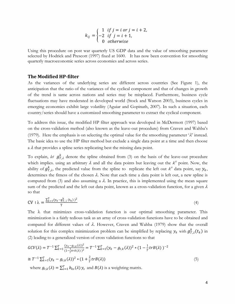
𝑘𝑖𝑗 = 1 𝑖𝑓 𝑗 = 𝑖 𝑜𝑟 𝑗 = 𝑖 + 2,

−2 𝑖𝑓 𝑗 = 𝑖 + 1, 0 𝑜𝑡𝑕𝑒𝑟𝑤𝑖𝑠𝑒

Using this procedure on post war quarterly US GDP data and the value of smoothing parameter selected by Hodrick and Prescott (1997) fixed at 1600. It has now been convention for smoothing quarterly macroeconomic series across economies and across series.

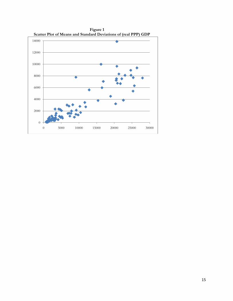
The Modified HP-filter As the variances of the underlying series are different across countries (See Figure 1), the

anticipation that the ratio of the variances of the cyclical component and that of changes in growth

of the trend is same across nations and series may be misplaced. Furthermore, business cycle

fluctuations may have moderated in developed world (Stock and Watson 2003), business cycles in

emerging economies exhibit large volatility (Aguiar and Gopinath, 2007). In such a situation, each

country/series should have a customized smoothing parameter to extract the cyclical component.

To address this issue, the modified HP filter approach was developed in McDermott (1997) based

on the cross-validation method (also known as the leave-out procedure) from Craven and Wahba‟s

(1979). Here the emphasis is on selecting the optimal value for the smoothing parameter „‟ instead.

The basic idea to use the HP filter method but exclude a single data point at a time and then choose

a that provides a spline series replicating best the missing data point.

To explain, let 𝑔𝑇,𝑘 denote the spline obtained from (3) on the basis of the leave-out procedure

which implies. using an arbitrary and all the data points but leaving out the kth point. Now, the

ability of 𝑔𝑇,𝑘 , the predicted value from the spline to replicate the left out kth data point, say 𝑦𝑘 ,

determines the fitness of the chosen . Note that each time a data point is left out, a new spline is

computed from (3) and also assuming a . In practice, this is implemented using the mean square

sum of the predicted and the left out data point, known as a cross-validation function, for a given so that

CV⃓ = (yk −gT,λ

k (tk ) )2Tk =1

T (4)

The that minimizes cross-validation function is our optimal smoothing parameter. This

minimization is a fairly tedious task as an array of cross-validation functions have to be obtained and

compared for different values of . However, Craven and Wahba (1979) show that the overall

solution for this complex minimization problem can be simplified by replacing 𝑦𝑘 with 𝑔𝑇,𝑘 (𝑡𝑘) in

(2) leading to a generalized version of cross validation functions so that

𝐺𝐶𝑉 𝜆 = 𝑇−1 (𝑦𝑘−𝑔𝑡 ,𝑘 𝜆 )2

(1−1

𝑇𝑡𝑟𝐴 (𝜆) )2

𝑇𝑘=1 = 𝑇−1 (𝑦𝑘 − 𝑔𝑡 ,𝑘 𝜆 )2 ∗𝑇

𝑘=1 (1 −1

𝑇𝑡𝑟𝐵(𝜆) )−2

≅ 𝑇−1 (𝑦𝑘 − 𝑔𝑡 ,𝑘 𝜆 )2 ∗𝑇𝑘=1 (1 +

2

𝑇𝑡𝑟𝐵(𝜆)) (5)

where 𝑔𝑡 ,𝑘(𝜆) = 𝑏𝑘𝑠(𝜆)𝑇𝑠=1 𝑦𝑠 and 𝐵(𝜆) is a weighting matrix.

5

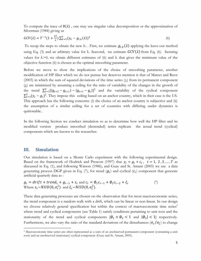
To compute the trace of 𝐵(𝜆) , one may use singular value decomposition or the approximation of Silverman (1984) giving us

𝐺𝐶𝑉 𝜆 = 𝑇−1(1 +2𝑇

𝜆) (𝑦𝑘 − 𝑔𝑡 ,𝑘 𝜆 )2𝑇

𝑘=1 (6)

To recap the steps to obtain the new : . First, we estimate 𝑔𝑡 ,𝑘 𝜆 applying the leave-out method

using Eq. (3) and an arbitrary value for . Seecond, we estimate 𝐺𝐶𝑉 𝜆 from Eq. (6). Iterating

values for >0, we obtain different estimates of (6) and that gives the minimum value of the

objective function (6) is chosen as the optimal smoothing parameter.

Before we move to show the implications of the choice of smoothing parameter, another

modification of HP filter which we do not pursue but deserves mention is that of Marcet and Ravn

(2003) in which the sum of squared deviations of the time series (yt) from its permanent component

(gt) are minimized by assuming a ceiling for the ratio of variability of the changes in the growth of

the trend [ gt+2 − gt+1 − gt+1 − gt ]2𝑇𝑡=1 and the variability of the cyclical component

{𝑦𝑡 − 𝑔𝑡}2𝑇𝑡=1 . They impose this ceiling based on an anchor country, which in their case is the US.

This approach has the following concerns: (i) the choice of an anchor country is subjective and (ii)

the assumption of a similar ceiling for a set of countries with differing under dynamics is

quitionable..

In the following Section we conduct simulation so as to determine how well the HP filter and its

modified version produce smoothed (detrended) series replicate the actual trend (cyclical)

components which are known to the researcher.

III. Simulation

Our simulation is based on a Monte Carlo experiment with the following experimental design. Based on the framework of Hodrick and Prescott (1997) that 𝑦𝑡 = 𝑔𝑡 + 𝑐𝑡 , 𝑡 = 1, 2 , 3 , … , 𝑇 as discussed in Eq. (1), and following Watson (1986), and Guay and St. Amant (2005) we use a data

generating process DGP given in Eq. (7), for trend (𝑔𝑡 ) and cyclical (𝑐𝑡 ) component that generate artificial quarterly data as :

𝑔𝑡 = 𝑑𝑟𝑖𝑓𝑡 + 𝑡𝑟𝑒𝑛𝑑𝑡 + 𝑔𝑡−1 + 𝜀𝑡 and 𝑐𝑡 = ∅1𝑐𝑡−1 + ∅2𝑐𝑡−2 + 𝜉𝑡 (7)

Where 𝜀𝑡~𝑁𝐼𝐼𝐷(0, 𝜎𝜀2) and 𝜉𝑡~𝑁𝐼𝐼𝐷(0, 𝜎𝜉

2).

These data generating processes are chosen on the observation that for most macroeconomic series,

the trend component is a random walk with a drift, which can be linear or non-linear. In our design

we choose relatively general specification but within the context of macroeconomic time series5

where trend and cyclical components (see Table 1) satisfy conditions pertaining to unit root and the

stationarity of the trend and cyclical components [∅1 + ∅2 < 1 and ∅2 < 1] respectively.

Furthermore, we also vary the ratio of the standard deviations of the disturbances (𝜎𝜀 𝜎𝜉 ) to change

5 Macroeconomic time series are often represented as a sum of an unobserved permanent component (containing a unit root) and an unobserved (stationary) cyclical component (Guay and St. Amant, 2005).

6

the relative importance of the trend and cyclical component because business cycle fluctuations may

be „moderate‟ in developed countries (Stock and Watson, 2003) compared to emerging economies

(Aguiar and Gopinath, 2007). By considering all the possibilities for the ratio6 of the standard

deviations of 𝜀𝑡 and 𝜉𝑡 (to be greater than, equal to, and less than unity) we allow predominance of

trend component over the cyclical one and vice versa.

We then generate 200 observations from equation (7) based on relevant parameter values given in

Table 1. This length is assumed to represent 50 years worth of quarterly data. Since most of the

macroeconomic data are heavily time aggregated (see Aadland, 2005), we also introduce time

aggregation7 to convert high frequency (quarterly) data to low frequency (annual) data. For this part

of simulation our time dimension reduces to one-fourth i.e. 50.

Once the series has been generated, we extract cyclical component by using a) the modified HP filter

where the (endogenous) value of lambda is based on the estimation process described above; and b)

the HP filter where the (exogenous) value of lambda is 1600 for data imagined as being generated at

quarterly frequency and is 100 for temporally aggregated (as annual) data. We repeated this

experiment 1000 times.

An ideal filter would extract the permanent (cyclical) component in such a manner that the mean

square error (MSE) of the extracted component and the one generated by (7) would be zero. To

assess and compare the performance of the modified HP filter and HP filter, we compare the MSE

of the permanent (cyclical) component extracted by the two filters.

In Table 1 we show the results of the performance of the modified HP filter and the HP filter by

comparing the mean square errors. Modified HP filter dominantly out-performs the HP filter in our

simulation study; including for the time aggregated data.

In the next Section, we apply the conventional and modified HP filters to observed data of a large

set of countries and then analyze afresh various important univariate and multivariate features of

cyclical series obtained by using these filters. But first we describe these data.

IV. Data

The empirical evaluation of a RBC model typically requires matching model moments with the relevant detrended macro series. The common practice is to compare the autoregressive coefficients and unconditional correlations of relevant series. These steps determine the fit of the model. Here we focus the extent to which autoregressive coefficients and their unconditional correlations are affected by the choice of the filtering method.

6 Values of this ratio (at 10, 1, and 0.5) are taken from Guay and St. Amant (2005). 7 There are three possibilities for converting the high frequency (quarterly) data to low frequency (annual) data. It may be systematic like in case of consumer price index (stock type data where we take end points), or by summing as in case of consumption (flow type data where we usually sum) or by averaging like in case of growth rate (rates type data where we usually average)).

7

To do so, we use quarterly (seasonally adjusted) and annual series of real GDP, real private consumption and real investment from International Financial Statistics database. The data are then transformed in logarithms. The data span for each country is mixed. Indeed for annual frequency, 93 countries have the relevant data series with some countries going as far back as 1950 while others only 1990. For quarterly frequency, data availability is scarcer. All in all 25 countries have the relevant quarterly data from a single source. Most series end at 2010 and our shortest data span is twenty years. The sample periods and the country lists for annual and quarterly series are reported in Table 2.

V. Empirical Results

In Table 2, we report the values of lambdas estimated from the modified HP filter from Eq. 6 for 93 (25) countries‟ annual (quarterly) real income, consumption and investment series. Three observations deserve highlighting. First, across countries and series for both annual and quarterly datasets there is an important level difference in the smoothing parameters. Second, for quarterly data the estimated cross country and series range for λ is 229-4898. This range is not too dissimilar from Agenor et al (1998)‟s range of 380-5100. However, their study was limited to 12 countries. Third, for the annual data the range is 11-6566. Fourth, relatively few countries fall close to the conventionally used λ=100 for annual and λ=1600 for quarterly series. Given the level differences in λs, it is important to establish the extent to which these impact the empirical moments of series; a task we turn to next.

To do so, first we obtain (for 93 countries) the first order autoregressive coefficients, standard errors, and the unconditional correlation of relevant series using the two filtering methods. For the first filtering method, detrending is based on using the modified HP filter with endogenously determined λs per country per series. For the second method, the conventional wisdom is applied by fixing λ=100 (1600) for annual (quarterly) frequency for all series and countries. Each set contains data on real income, real consumption and real investment. Second we use the detrended series to obtain the AR1 coefficient and unconditional correlations and carry out coefficient equality tests (see Paternoster et al. (1998)). Although we carry out multiple tests, we only report the results of Fisher Z-test for correlation.

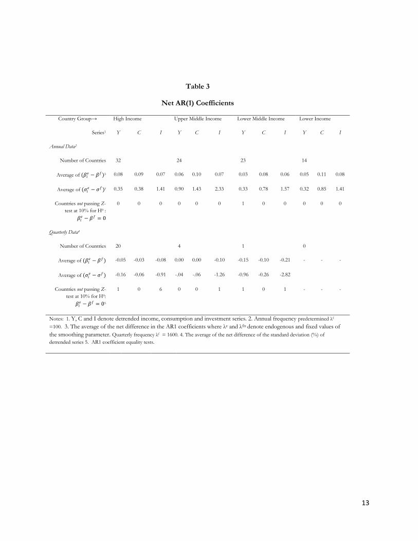
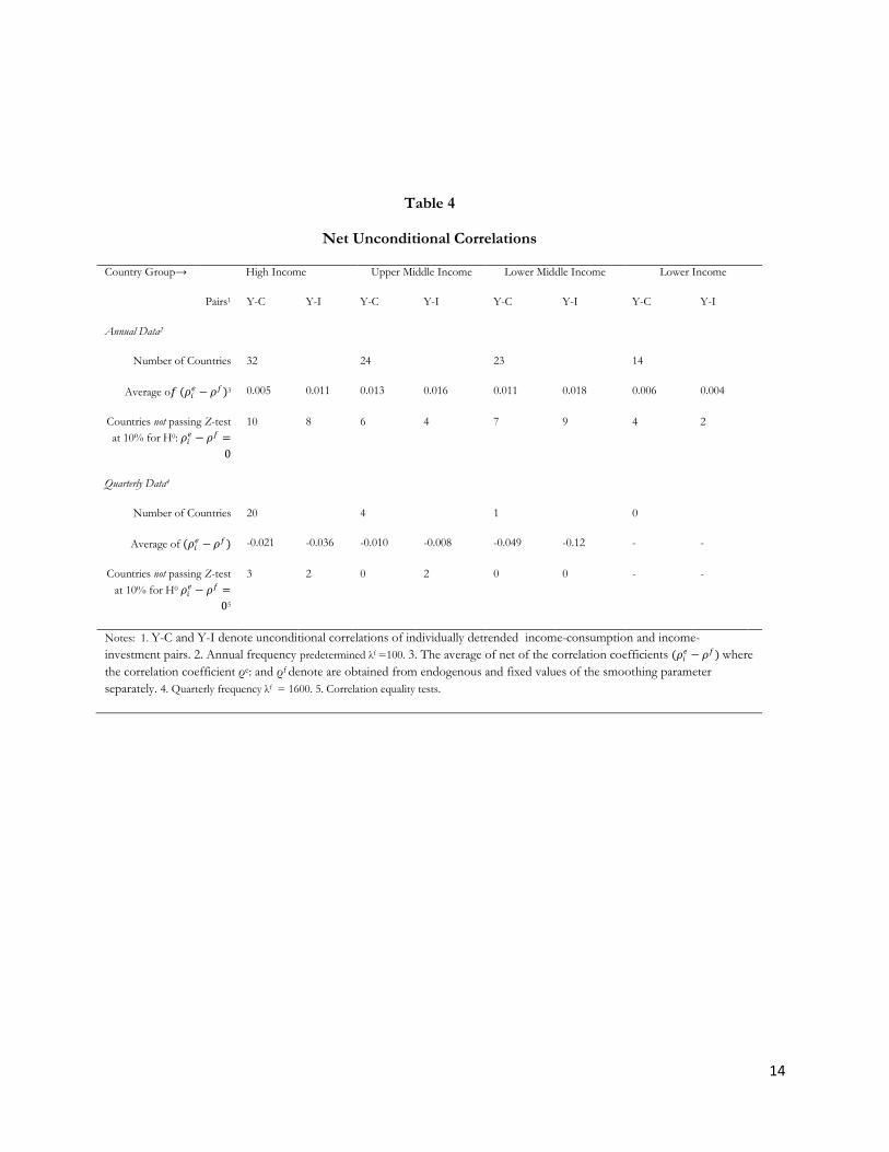
In Tables 3 and 4 we present a summary of our results by country based on their income brackets. The former table is devoted to feature individual series and while the latter Table presents differences in cross correlations. We discuss each in turn.

In terms of the individual detrended series there are three noticeable observations in Table 3. First, we find that on average net differences of standard deviations of detrended components of same series but from the two methods (where λ is first endogenous, then exogenous) are positive across countries and frequencies; i.e. detrended series using endogenous λs are more volatile. This result is in sync with the observation of Marcet and Ravn (2003) that too much variability is assigned to the permanent component when the cyclical component is extracted using the conventional HP filter approach. Second, the AR1 coefficients based on detrended series obtained from conventional method of fixing λs tends to give results that are biased downwards. Third, a statistical comparison (only Z-tests for coefficient equality are reported) of AR1 coefficients of same series but originating from the two methods reveal that coefficients are not too different from one another across country

8

groups and data frequencies. Therefore, in term of levels of persistence8 of our detrended macroeconomic series the choice of the λ appears immaterial - a result also found in our simulations.

Next, we turn to comparison of unconditional correlation in Table 4 from the two sets of data. For this purpose we apply the correlation-equality Fisher Z test of Bundick (1975)9. There are three important noteworthy findings. First, the point estimates of annual correlation coefficients between the cyclical components (extracted by modified HP filter) of the income-consumption and income-investment pairs are marginally higher as evidenced by the positive averages (across countries) of net of method-wise correlation coefficients. However, the opposite is true for quarterly correlations where the averages of net of method-wise correlation coefficients are negative. Second, although point estimate difference between pair-wise correlations emanating from our datasets is small, some of these differences appear to be statistically strong. Indeed, for a bigger set of countries within each country group the differences are empirically valid. This result is stronger for annual rather than quarterly correlation coefficients where about 1/3rd of countries in each income group reveal statistically different pair-wise correlations.

Thus, an important lesson to draw from our study is that the choice of λ is relevant. Thus, for business cycle research it is worthwhile to examine results using detrended series from endogenously determined λs.

VI. Concluding Remarks

As the use of business cycle knowledge becomes commonplace, a basic question on the choice of smoothing parameter for detrending macro series arises. In a simulation study we find that modified HP filter of McDermott (1997) performs better than Hodrick and Prescott (1997) filter in producing the generated permanent (cyclical) component under various definitions of permanent and cyclical components relevant to macroeconomic time series. We find the same result for the time aggregated cases as well.

In an empirical assessment, where we estimated λs for three core macroeconomic series of 93 countries with annual data and 25 countries with quarterly data using modified HP filter approach, we find that smoothing parameters differs across countries and frequency of data substantially. We do not find statistical differences in the AR1 coefficients of cyclical series either extracted using the modified HP filter or the traditional one that relies on fixing λs. A similar pattern is observed for pair-wise correlations of macroeconomic series generated from the two detrending methods and quarterly data. However, we find that the method of detrending tends to make more of a difference for annual series and multivariate analysis; though in this paper the multivariate analysis is restricted to unconditional correlation coefficients.

8 We also experimented with the autoregressive coefficients up to order 5 and our conclusions do not change. 9 See Yu and Dunn (1982).

9

References:

Aaland, David, (2005), Detrending Time-aggregated data, Economic Letters, 89, 287-93.

Agenor, P. R., McDermott, C. J. and Prasad, S. S. (1999), Macroeconomic Fluctuations in Developing Countries: Some Stylized Facts, International Monetary Fund Working Paper, 35.

Aguiar, M. and G. Gopinath (2007), “Emerging Market Business Cycle: The Trend is the Cycle,” Journal of Political Economy, Volume 115, pp 69-102

Backus, D. K. and Kehoe, P. J. (1992), International Evidence on the Historical Properties of Business Cycles, American Economic Review, 82, 864-88.

Baxter, M. and King, R. G. (1999), Measuring Business Cycles: Approximate Band-Pass Filters For Economic Time Series, Review of Economics and Statistics, 81, 575–93.

Bundick, L. E. (1975), Comparison of Tests of Equality of Dependent Correlation Coefficients, Ph.D. dissertation, University of California, Los Angles, USA.

Burns, A. F. and Mitchell, W. C. (1946), Measuring Business Cycles: New York, National Bureau of Economic Research

Cooley, T. F. and Ohanian, L. E. (1991), The Cyclical Behavior of Prices, Journal of Monetary Economics, 28, 25-60.

Correia, I., Neves, J. C. and Rebelo, S. (1992), Business Cycles in Portugal: Theory and Evidence, in J. Amaral, D. Lucena, and A. Mello (eds.) The Portuguese Economy Towards 1992, Springer, 1-64.

Guay, A. and St-Amant, P.(2005), Do the Hodrick-Prescott and Baxter-King Filters Provide a Good Approximation of Business Cycles, Annals of Economics and Statistics, No.77,pp 133-155.

Hodrick, R. J. and Prescott, E. C. (1997), Postwar U.S. Business Cycles: An Empirical Investigation, Journal of Money, Credit and Banking, 29, 1-16.

King, R. G. and Rebelo, S. T. (1993), Low Frequency Filtering and Real Business Cycles, Journal of Economic Dynamics and Control, 17, 1-2, 207-231.

McDermott, C. J.(1997), An Automatic Method for Choosing the Smoothing Parameter in the HP Filter,” unpublished, International Monetary Fund (June 1997).

Marcet, A. and Ravn, M. O. (2003), The HP-Filter in Cross Countries Comparisons, CEPR Working Paper No. 4244.

Paternoster, R., Brame, R., Mazerolle, P., and Piquero, A. (1998), Using the Correct Statistical Test for the Equality of Regression Coefficients, Criminology, 36, 4, 711-898.

Pedersen, T. M. (2001), The Hodrick-Prescott Filter, the Slutzky Effect, and the Distortionary Effect of Filters, Journal of Economic Dynamics and Control, 25, 1081-1101.

Ravn, M. O. and Uhlig, H. (2002), On Adjusting the Hodrick-Prescott Filter for the Frequency of Observations, The Review of Economics and Statistics, 84, 2, 371-376.

Silverman, B. W. (1984), A Fast and Efficient Cross- Validation Method for Smoothing Parameter Choice in Spline Regression, Journal of the American Statistical Association, 79, 387, 584-589.

Stock, J. H., and M. W. Watson (2003), Understanding Changes in International Business Cycle Dynamics, Working Paper No. w9859 (July), NBER, Cambridge

Yu, M. C. and Dunn, O. J. (1982), Robust Tests for the Equality of two Correlation Coefficients: A Monte Carlo Study, Educational and Psychological Measurement, 42, 4, 987-1004.

Watson, M.W.(1986), Univariate Detrending Methods with Stochastic Trends, Journal of monetary economics, No. 18,

pp 49-75

10

Appendix

Tables 1

Simulation Results of Performance Comparison of modified HP filter and HP filter Scenario Standard

deviation ratio

(𝜎𝜀

𝜎𝜉 )

AR coefficient Percent of times when modified HP filter outperforms HP filter

First

(∅1)

Second

(∅2) (Generated as)

Quarterly

Time Aggregated (Annual)

Linear

trend

Non-

linear

trend

Systematically By Summing By Averaging

Linear trend

Non-linear trend

Linear trend

Non-linear trend

Linear trend

Non-linear trend

1 10 0.9 0.01 100 100 100 100 100 100 100 100

2 10 1.2 -0.25 100 100 100 100 100 100 100 100

3 10 1.2 -0.4 100 100 100 100 100 100 100 100

4 10 1.2 -0.55 100 100 100 100 100 100 100 100

5 10 1.2 -0.75 100 100 100 100 100 100 100 100

6 5 0.9 0.01 100 100 100 100 100 100 100 100

7 5 1.2 -0.25 100 100 100 100 100 100 100 100

8 5 1.2 -0.4 100 100 100 100 100 100 100 100

9 5 1.2 -0.55 100 100 100 100 100 100 100 100

10 5 1.2 -0.75 100 100 100 100 100 100 100 100

11 1 0.9 0.01 100 100 100 100 100 100 100 100

12 1 1.2 -0.25 90 100 100 100 100 100 100 100

13 1 1.2 -0.4 100 100 100 100 100 100 100 100

14 1 1.2 -0.55 100 100 100 100 100 100 100 100

15 1 1.2 -0.75 100 100 100 100 100 100 100 100

16 0.5 0.9 0.01 90 100 100 100 100 100 100 100

17 0.5 1.2 -0.25 69 100 100 100 100 100 100 100

18 0.5 1.2 -0.4 100 100 100 100 100 100 100 100

19 0.5 1.2 -0.55 100 100 100 100 100 100 100 100

20 0.5 1.2 -0.75 100 100 100 100 100 100 100 100

21 0.01 0.9 0.01 100 100 100 100 100 100 100 100

22 0.01 1.2 -0.25 100 100 100 100 100 100 100 100

23 0.01 1.2 -0.4 100 100 100 100 100 100 100 100

24 0.01 1.2 -0.55 100 100 100 100 100 100 100 100

25 0.01 1.2 -0.75 100 100 100 100 100 100 100 100

26 10 0.8 0 100 100 100 100 100 100 100 100

27 5 0.8 0 100 100 100 100 100 100 100 100

28 1 0.8 0 100 100 100 100 100 100 100 100

29 0.5 0.8 0 100 100 100 100 100 100 100 100

30 0.01 0.8 0 100 100 100 100 100 100 100 100

11

Table 2 Smoothing Parameter based upon Modified HP Filter for Annual and Quarterly Data Series

Income Group Country Frequency Time Period Real GDP

λ

Real Consumption

λ

Real Investment

λ Start End

High Income

Australia Annual 1959 2010 363 278 412 Quarterly Q1-1959 Q4-2010 1398 3306 1051

Austria Annual 1964 2010 177 249 183 Quarterly Q1-1964 Q4-2010 921 2665 2074

Bahrain Annual 1975 2009 948 133 260 Belgium Annual 1953 2010 207 223 515

Quarterly Q1-1980 Q4-2010 669 885 816

Canada Annual 1950 2010 540 1280 860 Quarterly Q1-1957 Q4-2010 867 1054 506

Denmark Annual 1966 2010 203 620 798 Quarterly Q1-1977 Q4-2010 654 637 452

Finland Annual 1960 2010 504 279 566 Quarterly Q1-1970 Q4-2010 421 1885 571

France Annual 1959 2010 188 222 287 Quarterly Q1-1970 Q4-2010 476 818 283

Germany Annual 1960 2010 192 215 382 Quarterly Q1-1960 Q4-2010 1035 1040 489

Greece Annual 1958 2010 351 614 1482 Hungary Annual 1970 2010 90 59 97 Iceland Annual 1960 2010 593 745 666 Ireland Annual 1950 2010 91 411 140

Israel Annual 1981 2010 1079 1526 109

Quarterly Q1-1980 Q4-2010 2802 3216 892

Italy Annual 1960 2010 222 235 310 Quarterly Q1-1980 Q4-2010 602 863 627

Japan Annual 1955 2010 347 404 290 Quarterly Q1-1957 Q4-2010 1092 2633 630

Korea Annual 1953 2010 317 443 482

Quarterly Q1-1960 Q4-2010 2357 3576 1623

Luxembourg Annual 1985 2010 136 98 213 Malta Annual 1954 2007 101 91 674

Netherlands Annual 1980 2010 112 102 156

Quarterly Q1-1977 Q4-2010 414 602 568

New Zealand Annual 1954 2010 462 584 951 Quarterly Q2-1987 Q4-2010 356 416 311

Norway Annual 1966 2010 173 675 525 Quarterly Q1-1966 Q4-2010 1365 830 1146

Poland Annual 1981 2010 1493 501 1632 Portugal Annual 1977 2010 225 1059 442 Qatar Annual 1980 2010 152 87 305

Singapore Annual 1960 2009 393 205 420

Spain Annual 1956 2010 345 484 227

Quarterly Q1-1970 Q4-2010 1527 3346 1491

Sweden Annual 1950 2010 320 402 589

Quarterly Q1-1980 Q4:2010 656 834 284

Switzerland Annual 1950 2010 335 250 461

Quarterly Q1-1970 Q4-2010 503 1605 334

Trin & Tobago Annual 1966 2001 28 142 177

U.K. Annual 1950 2010 479 343 946

Quarterly Q1-1957 Q4-2010 1040 1229 1013

U.S. Annual 1950 2009 491 332 1754

Quarterly Q1-1957 Q1-2010 941 841 488

Upper Middle Income

Anguilla Annual 1984 2009 210 4592 484

Antigua Annual 1977 2010 294 495 577

Argentina Annual 1989 2010 52 166 168

Chile Annual 1974 2010 601 342 302

Costa Rica Annual 1961 2010 560 343 653

Dominican Rep. Annual 1962 2010 232 385 705

Ecuador Annual 1965 2010 199 408 220

Grenada Annual 1975 2010 188 214 190

Iran Annual 1966 2007 178 736 243

Jamaica Annual 1960 2009 130 219 205

Jordan Annual 1976 2007 40 49 683

Malaysia Annual 1970 2010 193 1687 606

Quarterly Q1-1991 Q4-2010 674 592 463

Mauritius Annual 1953 2010 984 964 1613

Mexico Annual 1978 2010 592 589 5656

Quarterly Q1-1981 Q4-2010 2671 2461 760

Continued on next page

12

Upper Middle Income

Country Frequency Time Period Real GDP

λ

Real Consumption

λ

Real Investment

λ Start End

Montserrat Annual 1977 2009 74 379 511

Panama Annual 1950 2009 336 517 517

Peru Annual 1989 2010 96 118 40

Quarterly Q3-1989 Q4-2010 1753 4898 704

South Africa Annual 1950 2010 299 722 289

Quarterly Q1-1960 Q4-2010 1316 1127 402

St Lucia Annual 1977 2010 179 1483 952

St Vincent/Grens Annual 1975 2010 321 6566 1392

Thailand Annual 1950 2010 217 350 496

Tunisia Annual 1961 2009 220 323 324

Uruguay Annual 1975 2010 184 185 184

Venezuela Annual 1977 2010 1624 390 451

Lower Middle Income

Belize Annual 1979 2008 298 161 894

Bhutan Annual 1980 2009 566 1026 166

Bolivia Annual 1984 2010 621 290 306

Cameroon Annual 1969 2006 11 73 56

Egypt Annual 1982 2009 367 273 390

El Salvador Annual 1990 2010 139 544 161

Fiji Annual 1968 2005 115 108 121

Guatemala Annual 1951 2010 98 220 399

Honduras Annual 1950 2010 512 252 599

India Annual 1960 2010 479 671 401

Indonesia Annual 1978 2010 147 288 78

Lesotho Annual 1980 2008 303 295 193

Mongolia Annual 1980 2005 51 168 185

Morocco Annual 1964 2009 413 198 365

Nigeria Annual 1969 2003 75 217 173

Pakistan Annual 1960 2010 104 240 481

Paraguay Annual 1962 2010 165 141 475

Philippines Annual 1958 2010 217 335 463

Quarterly Q1-1981 Q4-2010 229 621 329

Senegal Annual 1960 2009 690 1254 5162

Sri Lanka Annual 1950 2010 307 313 1478

Swaziland Annual 1977 2006 143 344 1174

Vietnam Annual 1990 2009 151 138 67

Zambia Annual 1972 2008 319 363 335

Lower Income

Bangladesh Annual 1973 2010 144 303 369

Benin Annual 1970 2006 651 239 519

Burundi Annual 1970 2010 86 253 149

Haiti Annual 1966 2007 211 381 285

Kenya Annual 1967 2010 411 374 295

Madagascar Annual 1980 2010 452 527 456

Myanmar Annual 1976 2003 51 77 76

Nepal Annual 1975 2010 247 458 977

Niger Annual 1986 2009 165 340 157

Rwanda Annual 1968 2010 720 611 410

Sierra Leone Annual 1971 2008 76 635 230

Togo Annual 1970 2004 1079 493 217

Uganda Annual 1983 2008 162 2565 420

Zimbabwe Annual 1980 2004 97 311 97

13

Table 3

Net AR(1) Coefficients

Country Group→ High Income Upper Middle Income Lower Middle Income Lower Income

Series1 Y C I Y C I Y C I Y C I

Annual Data2

Number of Countries 32 24 23 14

Average of (𝛽𝑖𝑒 − 𝛽𝑓)3 0.08 0.09 0.07 0.06 0.10 0.07 0.03 0.08 0.06 0.05 0.11 0.08

Average of (𝜎𝑖𝑒 − 𝜎𝑓)? 0.35 0.38 1.41 0.90 1.43 2.33 0.33 0.78 1.57 0.32 0.85 1.41

Countries not passing Z-

test at 10% for H0 :

𝛽𝑖𝑒 − 𝛽𝑓 = 0

0 0 0 0 0 0 1 0 0 0 0 0

Quarterly Data4

Number of Countries 20 4 1 0

Average of (𝛽𝑖𝑒 − 𝛽𝑓) -0.05 -0.03 -0.08 0.00 0.00 -0.10 -0.15 -0.10 -0.21 - - -

Average of (𝜎𝑖𝑒 − 𝜎𝑓) -0.16 -0.06 -0.91 -.04 -.06 -1.26 -0.96 -0.26 -2.82

Countries not passing Z-

test at 10% for H0:

𝛽𝑖𝑒 − 𝛽𝑓 = 05

1 0 6 0 0 1 1 0 1 - - -

Notes: 1. Y, C and I denote detrended income, consumption and investment series. 2. Annual frequency predetermined λf

=100. 3. The average of the net difference in the AR1 coefficients where λe and λfix denote endogenous and fixed values of

the smoothing parameter. Quarterly frequency λf = 1600. 4. The average of the net difference of the standard deviation (%) of

detrended series 5. AR1 coefficient equality tests.

14

Table 4

Net Unconditional Correlations

Country Group→ High Income Upper Middle Income Lower Middle Income Lower Income

Pairs1 Y-C Y-I Y-C Y-I Y-C Y-I Y-C Y-I

Annual Data2

Number of Countries 32 24 23 14

Average o𝑓 (𝜌𝑖𝑒 − 𝜌𝑓)3 0.005 0.011 0.013 0.016 0.011 0.018 0.006 0.004

Countries not passing Z-test

at 10% for H0: 𝜌𝑖𝑒 − 𝜌𝑓 =

0

10 8 6 4 7 9 4 2

Quarterly Data4

Number of Countries 20 4 1 0

Average of (𝜌𝑖𝑒 − 𝜌𝑓) -0.021 -0.036 -0.010 -0.008 -0.049 -0.12 - -

Countries not passing Z-test

at 10% for H0 𝜌𝑖𝑒 − 𝜌𝑓 =

05

3 2 0 2 0 0 - -

Notes: 1. Y-C and Y-I denote unconditional correlations of individually detrended income-consumption and income-

investment pairs. 2. Annual frequency predetermined λf =100. 3. The average of net of the correlation coefficients (𝜌𝑖𝑒 − 𝜌𝑓) where

the correlation coefficient ρe: and ρf denote are obtained from endogenous and fixed values of the smoothing parameter

separately. 4. Quarterly frequency λf = 1600. 5. Correlation equality tests.

15

Figure 1 Scatter Plot of Means and Standard Deviations of (real PPP) GDP

0

2000

4000

6000

8000

10000

12000

14000

0 5000 10000 15000 20000 25000 30000