MPRAMunich Personal RePEc Archive

Identifying regime shifts in Indian stockmarket: A Markov switching approach

Ahmad Wasim and Kamaiah Bandi

Department of Financial Studies, University of Delhi, India, 110 021,Department of Economics, University of Hyderabad, India, 500 046

11. January 2011

Online at https://mpra.ub.uni-muenchen.de/37174/MPRA Paper No. 37174, posted 8. March 2012 00:45 UTC

1

Identifying regime shifts in Indian stock market: A Markov switching approach

Wasim Ahmad*1

, Bandi Kamaiah**

* Department of Financial Studies, University of Delhi, India, 110 021

** Department of Economics, University of Hyderabad, India, 500 046

Abstract

Seeking for the existence of bull and bear regimes in the Indian stock market, a two state

Markov switching autoregressive model (MS (2)-AR (2)) is used to identify bull and bear

market regimes. The model predicts that Indian stock market will remain under bull regime

with very high probability compared to bear regime. The results also identify the bear phases

during all major global economic crises including recent US sub-prime (2008) and European

debt crisis (2010). The paper concludes that the Indian stock market is more sensitive to

external shocks implying that there is ample scope of policy interventions.

Keywords: Markov switching model, Stock returns, Regime shifts

JEL Classification: C32, C51

1 Corresponding author, Tel: +91- 98 73 46 84 97

Email: ahmadwasimdu@gmail.com

2

1. Introduction

It is empirically proved that financial market exhibits upward and downward trends which in

common terminology is categorized as bull and bear market. However, there is no clear

classification of stock market regimes i.e. bull or bear in the literature but few studies by

Fabozzi and Francis (1977), Kim and Zumwalt (1979) and Chen (1982) have defined bull

regime on the basis of returns exceeding certain threshold value. The occurrence of these

regimes is often attributed to several factors that can be broadly grouped into systematic and

non-systematic risks. A bull regime is generally characterized as periods of generalized

upward trend (positive returns with low volatility) and bear market corresponds to periods of

generalized downward trend (negative returns with considerably high volatility). The

identification of regime shifts has great significance in making portfolio allocation strategies

and enable policy makers to undertake the timely measures to curb on speculative activities.

Besides these risks, changes in the regime in a stock market can be due to external shocks

caused by a shock in another market. The obvious examples are Asian flu (1997), Russian

cold (1998), Brazilian fever (1999), NASDAQ rash (2000), Argentinean crisis (2001/02),

Sub-prime crisis (2008) and the most recent European Sovereign debt crisis (2010). These

incidents had catastrophic impacts on stock market regimes around the world including India

and the markets were revived through policy interventions. Keeping this in view, the present

study attempts to highlight the dynamics of Indian stock market, in particular, identifying bull

and bear regimes in two leading indices viz., NSE-Nifty and BSE-Sensex. We apply a

probability based Markov-switching model for returns in which the distribution of returns

changes over time, i.e., the time-series tends to be cyclical, for example, due to business

cycles or stock market cycles (bull and bear). Markov-switching (MS) models are

characterized by transitions between states which are governed by a Markov chain. Our study

3

uses a Markov regime switching model which jointly characterizes the unobservable bull and

bears regimes for stock returns, allows intra-regime dynamics, dating and enables further to

model the uncertainty about the market regime to be incorporated into out-of-sample

forecasts. These apart, it is empirically proved that stock market reflects behaviour such as

sudden jumps and crash and therefore, this study also highlights the significance of the use of

non-linear MS-AR model compared to linear AR model in case of Indian stock market.

2. Literature Review

Numerous studies have applied Markov regime switching model in identifying the regime

switching behaviour of stock market. The first among these studies is that of Hamilton (1989)

who enhanced the model of Goldfeld and Quandt (1973) by allowing the regime shifts in

dependent data and developed the Markov switching autoregressive model (MS-AR). Since

then, the model has been used extensively to capture the regime switching behaviour in

economic and financial time series studies. However, the application of Markov regime

switching model in financial econometrics, particularly in identifying the regime shifts,

started with the pioneer work of Turner et al. (1989) to capture the regime shifts behaviour in

stock market using MS-AR () model. Their study highlighted the usefulness of Markov

switching model allowing regime shifts to happen in mean and variance and fitting the data

adequately compared to other specifications of Markov regime switching models. Cheu et al.

(1994) examined the relationship between stock market returns and stock market volatility

using the MS-AR model and concluded that there is nonlinear and asymmetric relationship

between returns and volatility. Schaller and Norden (1997) carried out a study similar to the

Turner et al. (1989) in several directions and found a strong regime switching behaviour in

the stock market returns. Nishiyima (1998) investigated the existence and nature of different

regimes in aggregate stock returns of five industrialized countries. His study exhibited regime

4

shifts in volatility rather than in mean returns in five countries. He concluded that volatility

instead of mean returns reveal regime shift behavior in all countries.

Maheu and McCurdy (2000) used the Markov regime switching model to classify the US

stock market in two different regimes characterized as high returns–stable-state and low

return-volatile-state. Guidolin and Timmerman (2006) applied MS-VAR approach to study

the relationship between US returns and bond yields. They concluded that four regimes MS-

VAR model is required to capture the time variation in the mean, variance and correlation

between stock returns and bond yields. Wang and Theobald (2007) carried out a study using

MS with switching–in-mean and variance model to investigate the regime switching volatility

in six East Asian emerging markets i.e., Indonesia, Korea, Malaysia, Philippines, Taiwan and

Thailand, from 1970 to 2004. They concluded that the markets for Malaysia, Philippines and

Taiwan were characterized by two regimes while the markets for Indonesia, Korea and

Thailand were characterized by three regimes over the sample period. Ismail and Zaidi

(2008) examined the regime shifts behaviour in Malaysian stock market returns using MS-

AR model. They implemented the MS-AR framework to capture regime shifts behaviour in

both mean and variance in four indices of Bursa Malaysia namely the Composite, Industrial,

Property and Financial indices. They successfully captured the regime shifts in each index

and concluded in favour of applying nonlinear MS-AR model against linear AR model.

Maheu et al. (2009) used Markov switching model in order to identify bull and bear regimes

for stock market returns. They used 123 years of daily returns on value weighted index of

NYSE, AMEX and NASDAQ and applied various structures of markov model to identify the

regime shifts and concluded in favour of application of Markov switching model in

indentifying regime shifts.

5

One of the first attempts using Markov switching model in case of India was by Laha (2006).

The study identified the regime switching behaviour of Indian stock market using Hidden

Markov models under Bayesian framework to address the problem of detecting and

predicting regime switching behaviour. Bhattacharya and Singh (2006) used Markov

switching model to explore unbiased expectations and efficient market hypothesis. They

concluded that relatively longer time horizon is more effective in eliminating arbitrage

opportunities than the short run. Kumar (2006) showed the relationship between stock price

and trading volume using Markov Switching Vector Error Correction Model (MS-VECM).

Using weekly data, He analysed the joint dynamics of stock price and trading volume and

concluded that for the whole of the study period, the adjustment towards long run occurs at

different rates under the two different regimes.

It is apparent from the above mentioned studies that there are evidences of regime switching

behaviour in stock market which can be better understood by applying non-linear models

such as markov regime switching model. In case of Indian stock market, very few studies

have been undertaken to address the dynamics of regime shifts. The present study will add

value to the existing literature in the following directions. We examine the regime switching

behaviour of Indian stock market with dating using daily data. Further, the study examines

whether stock market returns are predictable even after accounting for Markov switching

behaviour using forecasts of both regimes. The study also tries to compare the dating of both

leading indices with prediction of each regime. All these aspects of stock market regime

have been largely ignored by the existing studies in the case of India. Rest of the paper is

organized as follows. Section 3 outlines the methodology used for investigating the

objectives. Section 4 describes the data used for the study. Section 5 reports and analyses the

empirical results and section 6 ends with concluding remarks.

6

3. Methodology

The Markov Switching – Auto Regressive (MS-AR) approach is used in this study. This

approach is an extension of the AR () model to the nonlinear case. It assumes the existence of

a finite number of states, each of which is being characterized by an AR () model. The

Markov switching model assumes that time series may display periodic changes in their

observed behavior. Such changes happen through switches in states, where the data

generating process and average duration of each state are allowed to differ. Assume that tr is

time-series generated as an autoregression of order p with regime switching-in-mean and

variance.

2

1

( ) ( ( )) ( )p

t t i t i t i t t

i

r S r S S

…………………………(1)

Here, mean and variance 2 of the process depend on the regime at time t, indexed by tS a

discrete variable. i is the model parameter and t is an i.i.d N (0,1) random variable. tS is

assumed to be a n-state, first order Markov process, taking the values 1………n with

transition probability matrix:

P = { i jp } , 1,2.......i j n ;

Where, i jp = Pr[ 1| ]t tS j S i with 1

1n

ij

j

p

for all i ………… (2)

The state dependent mean and variances are specified as

1 1 ,( ) ...........t t n n tS S S …………………………………………..(3)

2 2 2

1 1 ,( ) ...........t t n n tS S S …………………………………………(4)

Where itS takes the value of one when tS is equal to i and two otherwise. Then equation (1)

can then be written as 1 1 ,..........t t n n t tr S S ……………………. (5)

7

2 2

1 1 ,

1

( ............... )p

t t i t n n t t

i

i S S

……………………………… (6)

Based on equation (2), two state transition probability matrix based on first order Markov

process can be represented by

Prob [ tS = 1| 1tS =1] = p11

Prob [ tS = 2| 1tS = 1] = 1-p11 = p12

Prob [ tS = 2| 1tS = 2] = p22

Prob [ tS =1| 1tS = 2] = 1- p22 = p21

With 11 12 21 22 1p p p p

In the above algorithm, p11 and p22 denote the probability of being in regime one, given that

the system was in regime one during the previous period, and the probability of being in

regime two given that the system was in regime two during the previous period, respectively.

Thus 1- p11 defines the probability that yt will change from state 1 in period t-1 to state 2 in

period t, and 1- p22 defines the probability of shift from state 2 to state1 between times t-1 and

t. Thus p12 is the probability of going from state 1 to state 2.

Details of the estimation and forecasts algorithms of MS model is well known and can be

found in Krolzig (1997, 2001) and Hamilton (1989, 1993a, 1993b, 1994).

4. Data

The daily data of two leading Indian stock market indices viz., NSE-Nifty and BSE-Sensex

have been taken for analysis, from 02-07-1997 to 12-11-2010 with total data points of 3303

of BSE-Sensex and 3319 of Nifty-fifty, respectively. It may be noted that in both the markets

opening days are not same. Therefore, regime cycles dating are not comparable in one to one

manner. But on an average the movements of these two indices could be compared

8

highlighting major shocks or events. Both the indices are analysed in returns.2 The main

reason for using the daily data is to identify more frequent regime switches in both indices

compared to low frequency data. Standard unit root tests (not reported but available upon

request) indicate that both data series are stationary.

5. Empirical results

Before applying the markov switching model, one has to decide, (i) the number of regimes,

(ii) model specification (changing means, variance and AR dynamics) and (iii) lag order of

the AR terms (not necessarily in this order). In practice, the state dimension of an MS model

is generally determined, either informally by visual inspection of the data or by statistically

sound procedures such as Likelihood ratio (LR) tests (e.g., Hansen 1992 and Garcia 1998)

and / or data-dependent model selection criteria (Psaradakis and Spagnolo 2003). However,

there are several problems with these approaches: the LR tests do not satisfy the standard

regularity conditions under the null hypothesis since some parameters are not identified.

Determining the number of regimes based on complexity-penalized likelihood criteria such as

the Akaike Information Criteria (AIC), the Hannan-Quin Information Criterion (HQIC) and

the Schwarz’ Bayesian Information Criterion (SIC) as suggested by Psaradakis and Spagnolo

(2003) is also problematic because one has to know, for certain, the AR lag order (and other

parameters), as well as the MS model specification simultaneously. Inclusion of too many

regimes where they are non-existent would result in spurious regressions and reduced

accuracy of parameter estimates and precision of forecasts. To avoid the problems of over

and under-fitting the state dimension as well as model misspecification. In this study, we

determine the number of states based on the visual inspection of the data without considering

information criteria. The choice of number of autoregressive terms are based up on serial

2 The returns are calculated by 1[{log( ) log( )}*100]t tr r

9

correlation present in both stock market series. A two-state Markov regime switching model

is applied. The MS (2)-AR (2) model has been estimated by employing the maximum

likelihood approach, for both Nifty and BSE-Sensex indices. The process indicated that the

strong convergence is achieved. The filtered and smooth probabilities for the two states are

obtained after estimation. The estimation results of the BSE-Sensex are presented in table 1.

[Insert table 1 about here]

From table 1, it can be seen that the AR (2) co-efficients are significant. Since regime 1 (St

=1) exhibits the negative returns with high volatility and St =2 indicates the negative returns

with low volatility. It implies that state 1 indicates bear regime and state 2 represents bull

regime in the estimated results of BSE and NSE. In the regime represented by St =1, the

average expected return is 1 = -0.177 percent per day with high volatility of 2

1 = 6.791,

while St =2, the average growth rate is 2 = 0.155 percent per day with low volatility

compared to bear regime as 2

2 = 1.214. The persistence of each regime is high.3 The

probability that the bear regime will be followed by another day of bear regime is p11 = 0.96

and the regime will persist, on average, for 26 days (more than a month). However, the

probability that the bull regime will be followed by another day of bull regime is p22 =

0.98.This episode will typically persist for 54 days (close to two months). It is interesting to

observe that during bear regime the average expected returns is negative with high volatility

compared to bull regime. Similarly, the probability that the bear regime will be followed by

bull phase is represented by p12 = 0.02 and the average persistence of this regime is only 1

day. The probability that the bull will be followed by another day of bear is p21 = 0.04 and the

average duration of this regime is 1 day. The results of these two regimes unravel the

3 The persistence of a particular regime is calculated using the formula of (1-pij)

-1, Where, i = 1, 2 and j = 1, 2

(in case of two state MS model).

10

interesting facts about the adjustment of bear/bull cycles in BSE-Sensex. The obvious

inference coming out from the estimation result is that the market is more biased towards bull

regime with very high persistence with positive returns and there is very high probability of

occurrence of extreme events. Transition phases are adjusted very quickly given the market

scenarios.

[Insert table 2 about here]

Similarly, table-2 shows the estimation results of MS (2)-AR (2) of NSE-Nifty index. It can

be observed that AR (2) co-efficients are significant. In the regime represented by St =1 (bear

phase), the average expected return in this regime is 1 = -0.19 percent per day with high

volatility of 2

1 = 6.66, while in case of bull phase represented by state 2 (St =2), the average

growth rate is 2 = 0.17 percent per day with low volatility of 2

2 = 1.21. Both regimes are

persistent with varying average durations. The probability that the bear regime will be

followed by another day of bear regime is p11 = 0.95, this regime will persist on average for

20 days (close to one month). However, the probability that the bull regime will be followed

by another day of bull regime is p22 = 0.97, this episode will typically persist for 39 days

(more than a month). It is interesting to observe that during bear regime the average expected

return is negative with high volatility compared to bull regime. If we compare the bear/bull

regime returns of both the markets, then it may be concluded that both markets show the

similar trends in returns with almost similar volatility in respective regimes of markets.

However, the transition phases of Nifty returns mentioned in table 2 shows the similar trend

of BSE-Sensex. In case of Nifty, the probability that the bear regime will be followed by bull

regime represented as 12p = 0.03 and the average duration of this regime will be only one

day. Conversely, the probability that the bull regime will be followed by bear regime is

11

represented as 21p = 0.05 with average persistence of 1 day. These results again unravel the

similar insights about the very low duration of transition phases in both the markets. The

reason could be the emerging nature of Indian economy wherein the market participants

follow the herd trend with longer period of holdings and sell the holdings in the case of

adverse economic conditions.

[Insert table 3 & 4 about here]

Further, the possible bull and bull regime dates for both stock market indices are obtained

from the smoothed probabilities (see table 3 & table 4). In case of BSE-Sensex, thirty three

(33) days of bear and bull regimes with varying durations have been identified (table 3). The

average durations of bull and bear regimes are sixty nine (69) and thirty two (32) days

respectively. The overall average duration of BSE-Sensex regimes is hundred (100) days.

While in Nifty case, there are fifty (50) bull and bear regimes with different durations are

shown in table 4. The average durations of bull and bear regimes are forty five (45) and

twenty two (22) days respectively. However, the overall average duration of Nifty cycle is

obtained as sixty six (66) days. If we compare the cycles durations between BSE-Sensex and

NSE-Nifty then we can conclude that the average duration of both the regimes are higher in

case of BSE-Sensex and even the overall average cycle’s phase by more than 30 days (1

month). The reason could be due to high diversification and volume of trade taking place in

BSE-Sensex than Nifty and also could be because of large listings of companies in BSE-

Sensex compared to Nifty.

It may, however, be noted that during the study period the longest bull regime in BSE-Sensex

is observed (see table 3) in cycle 23 (04-06-2004 to 10-05-2006) for 481 days (more than a

year), followed by cycle 19 (29-05-2002 to 22-08-2003) for 308 days. Whereas, the longest

bear regime is shown in cycle 30 (30-05-2008 to 24-07-2009) for 280 days. The longest

12

overall (bull and bear) cycle is observed in cycle 23 (04-06-2004 to 10-05-2006) for 535

days. Out of 535 days, 481 days are under bull regime and 54 days under bear regime.

Similarly, in case of Nifty (see table 4) during the study period the longest duration under

bull regime is found in cycle 25 (29-05-2002 to 08-04-2003) for 216 days followed by

varying periods between cycles 32 to 34 (07-06-2004 to 18-04-2006) for 152 days (on

average). However, the longest bear period in NSE-Nifty is observed in cycle 44 (11-08-2008

to 23-07-2009) for 229 days followed by cycle 16 (22-12-1999 to 05-06-2000) for 112 days.

The longest overall (bull and bear) cycle is observed in cycle 44 (11-08-2008 to 23-07-2009)

for 231 days, out of which 229 days are under bear and 2 days under bull regimes,

respectively.

This is, however, evident from the above analysis that both the markets move in more or less

similar direction with varying durations of each positive/negative shocks which lead the

market to either takes a jump or crash.

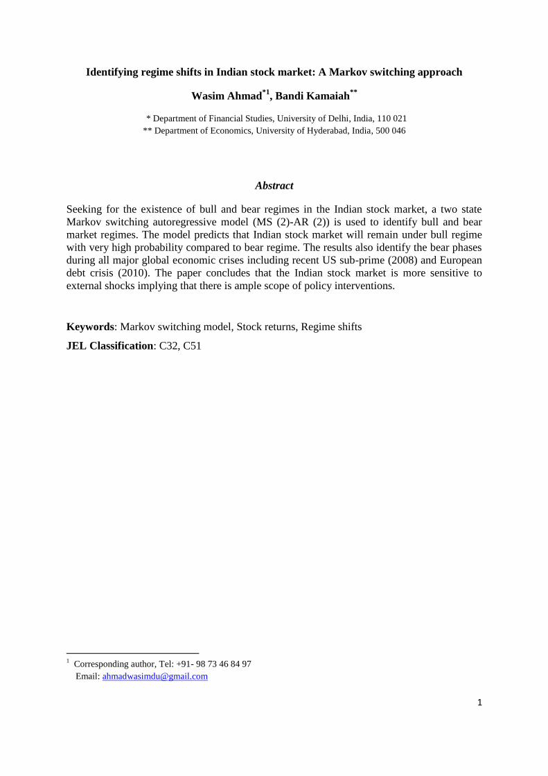
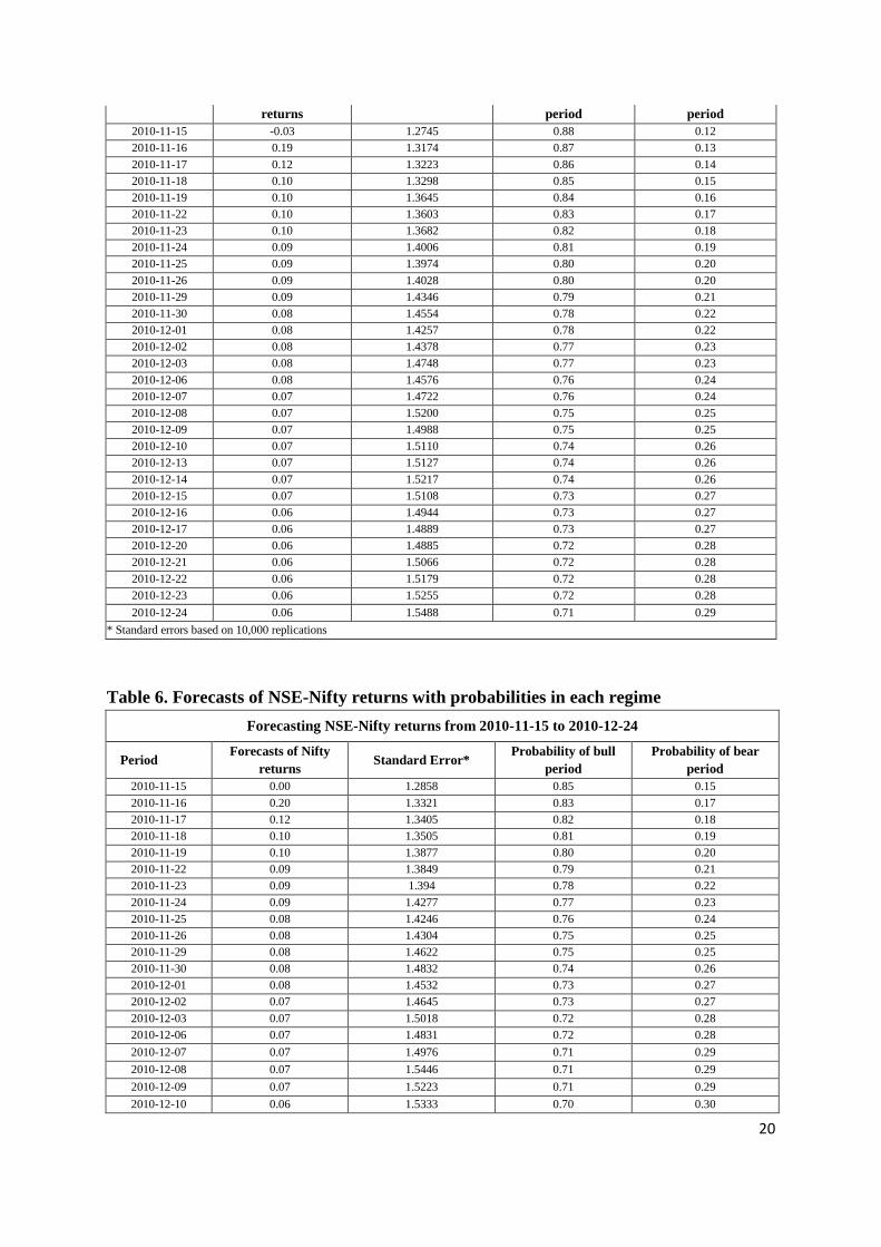
[Insert table 5 & 6 about here]

Apart from this, both market indices are forecasted (see table 5 & 6) further for the period of

one month (15-11-2010 to 24-12-2010). The main reasons for forecasting the returns series is

to have forward looking scenarios with given probabilities of each regime. In case of BSE-

Sensex, the forecasted returns are positive except one period (15-11-2010). The positive

returns are ranging between 0.06 to 0.19 percent per day with given probabilities of bull and

bear regimes. The inference coming out from the one month forecasts of BSE-Sensex is that

there is a tendency for the market to remain under the bull regime as evidenced by very high

probabilities ranging from 0.71 to 0.88 compared to the 0.12 to 0.29 range under the bear

regime.

13

Similarly, the forecasted returns of Nifty index are also falling in line with BSE-Sensex

index. As it can be observed that the forecasted Nifty returns are positive with given

probabilities of bull and bear regimes. The returns are varying between 0.0 to 0.20 percent

per day with given probabilities of the market remaining under bull regime with very high

probabilities ranging between 0.69 and 0.85 whereas bear regime is having very low

probability ranging from 0.15 to 0.32. After analysing the forecasted returns of both markets,

it may be inferred that the Indian stock market will remain under bullish regime with slight

moderation and meagre market correction in late December 2010 as it could be easily

observed by the given probabilities of the bear regime.

[Insert figure 1a & 1b about here]

[Insert figure 2a & 2b about here]

Another important insight coming out from this study is identifying durations of contagion in

Indian stock market during the US sub-prime crisis of 2008. As it can be seen in (Graph 1a &

1b) that India started realizing the contagion of sub-prime crisis in BSE-Sensex from May

2008 (30-05-2008) to July (24-07-2009). The average duration of the effect of sub prime in

case of BSE Sensex is 280 days. But in case of Nifty the smoothed probabilities (see Graph

2a, 2b) show that the sub-prime contagion started realizing from mid of August 2008 (11-08-

2008) and ended in July 2009 (23-07-2009) with average duration of 229 days. But the

impact of European crisis (2010) was not much visible which could be due to rising share

prices, strong investor interest, and sentiment of global recovery with little market

corrections; otherwise there is not very high duration of bear regime, implying that after the

contagion effects of US Sub-prime Indian stock market remained bullish due to large inflow

of capital in portfolio investment and heavy borrowing made by domestic corporations

through IPOs and FPOs. But the uncertainties arising due to fear of double deep-recession

14

and slow recovery observed in USA and Euro-zone economies has further abridged the

chances of strong global economic recovery. This might lead to chaos in Indian stock market

with the possibility of considerable market corrections ahead.

6. Concluding remarks

India as a developing economy with a growth rate of around nine percent per annum has

received considerable attention across the globe with heavy investment in all the sectors

opened so far for foreign investment. The post-liberalization period has particularly brought a

sea-change in financial sector with more technology driven market integration and pursuance

of aggressive deregulation policies. With the advent of new technology, the investment in

stock market has become a usual phenomenon with more inflow of capital moving from one

corner of the world to another in the fraction of a second. This has helped in enhancing the

efficiency of Indian stock market. But the risk of speculation associated with such

developments has become a major concern. The present study tries to provide a basic

framework to understand the dynamics of stock market behaviour and attempts to identify the

movements of stock market in different regimes characterized as bull and bear. Considering

the fact that prediction of the stock market trend guides the policy makers in undertaking

timely intervention and is a help to speculators to play safe and avoid losses, the study

estimates and forecast the MS (2)-AR (2) model for both leading indices (BSE-Sensex and

NSE-Nifty) of Indian stock market using daily data for the period July-1997 to December-

2010. The MS (2)-AR (2) model predicts that Indian stock market will remain under bull

regime with very high probability compared to the bear regime. The persistence of the bull

regime is more than one month in both the markets. The study results also highlight the bear

phases during sub-prime crisis (2008) which is more than a year with an average duration of

254 days in both market indices. But there is no evidence of severe effect of European Debt

15

crisis (2010) in both indices of Indian stock market. The one month forecasts of both the

market indices further substantiate the presence of similar trends of Indian stock market to

remain under bull regime with very high probabilities and slight moderation in late

decemeber-2010. Finally, the study concludes, in the backdrop of economic liberalization

policies, that Indian stock market in recent years has become more sensitive to external

shocks implying that there is ample scope of policy interventions. This is mainly because as

the economy treads a higher growth path and is subjected to greater opening and financial

integration with rest of the world, the stock markets in all its aspects need further

considerable attention, along with corresponding measures to continue modernization and

strengthening.

Acknowledgments

The authors acknowledge Md. Zulquar Nain, Biswajit Mohanty and Ritesh Kumar Mishra for

their valuable comments and suggestions on improving this paper.

References

Cecchetti, S., P. Lam., N. Mark. (2000). Asset Pricing with Distorted Beliefs: Are Equity Returns Too

Good to be True?, American Economic Review, 90(4), 787–805.

Chen, S. (1982). An examination of risk returns relationship in bull and bear markets using time varying

betas, Journal of Financial and Quantitative Analysis, 17,265–85.

Chu, C. S. J., Santoni, G. J., & Liu, T. (1996). Stock market volatility and regime shift in return.

Information Science 94: 179-190.

Fabozzi, F. J. and Francis, J. C. (1977). Stability tests for alphas and betas over bull and bear market

conditions, Journal of Finance, 32, 1093–99.

Garcia, R. (1998). Asymptotic null distribution of the likelihood ratio test in Markov switching model.

International Economic Review, 39, 763–88.

Garcia, R., & Perron, P. (1996). An analysis of the real interest rate under regime shifts. Review of

Economics and Statistics, 78,111-125.

Goldfeld, S. M., & Quandt. R. E. (1973). A Markov model for switching regressions, Journal of

Econometrics. 1, 3-16.

Gordon, S., & P. St-Amour. (2000). A Preference Regime Model of Bull and Bear Markets. American

Economic Review, 90(4), 1019–1033.

Guidolin, M., & A. Timmermann. (2002). International asset allocation with regime shifts. Review of

Financial Studies, 15, 1137–1187.

Guidolin, M., & A. Timmermann. (2005). Economic Implications of Bull and Bear Regimes in UK

Stock and Bond Returns. The Economic Journal, 115(111-143).

Guidolin, M., and A. Timmermann. (2008). International Asset Allocation under Regime Switching.

Skew, and Kurtosis Preferences. Review of Financial Studies, 21(2), 889-935.

16

Hamilton J.D and G.Lin (1996) Stock market volatility and business cycle. Journal of Applied

Econometrics, 11, 573-593.

Hamilton, J. D. (1994) Time Series Analysis, Princeton University Press, New Jersey.

Hamilton, J.D (1993a) Estimation, inference and forecasting of time-series subject to changes in

regime. in G.S.Maddala, C.S.Rao, and H.D.Vinod,eds., Handbook of Statistics, Vol.11. New

York: North-Holland.

Hamilton, J.D. (1993b). State-space models, in Robert Engle and Daniel McFadden. eds., Handbook of

Econometrics, Vol.4.New York: North-Holland.

Hamilton, J.D. (1989). A new approach to the economic analysis of non-stationary time series and the

business cycle. Econometrica, 57, 357-384.

Hansen, B. (1992). The likelihood ratio test under non-standard conditions: Testing the Markov

switching model of GNP. Journal of Applied Econometrics 7, S61–82.

Ismail Tahir Mohammed., & Isa Zaidi. (2008). Identifying regime shifts in Malaysian stock market

returns. International Research Journal of Finance and Economics, Issue 15, 2008.

Kim, M. K. & Zumwalt, J. K. (1979). An analysis of risk in bull and bear markets. Journal of

Financial and Quantitative Analysis, 15, 1015–25.

Krolzig, H.M. (1997). Markov-switching vector autoregressions: Modeling, statistical inference and an

application to the business cycle analysis. Lecture Notes.

Krolzig, H.M. (2001). Business cycle measurement in the presence of structural change: International

evidence. International Journal of Forecasting 17, 349–368.

Kumar Alok. (2006). A markov switching vector error correction model of the Indian stock price and

trading volume. IGIDR Working paper, 2006.

Laha Kumar Arnab. (2006). Analysis of regime switching behaviour of Indian stock market. Computing

in Economics and Finance, No 249.

Maheu, J. M. & Mccurdy, T. H. (2000). Identifying Bull and Bear markets in stock returns. Journal

of Business and Economic Statistics. 18, 100-112.

Nishiyima, K. (1998). Some evidence of regime shifts in international stock markets. Managerial

Finance 24(4), 30-55.

Psaradakis, Z., & N. Spagnolo. (2003). On the determination of the number of regimes in Markov-

switching autoregressive models. Journal of Time Series Analysis 24, no 2, 237–52.

Prasad, B., & Singh, H. (2006). Estimating forward pricing function: How efficient is Indian stock

index futures market. Accounting, Finance, Financial Planning and Insurance Series, No 2,

Deakin University.

Quandt, R. E., (1958). Estimation of the Parameters of a Linear Regression System Obeying Two

Separate Regimes. Journal of the American Statistical Association. 53, 873-880.

Schaller, H., & Norden, S. (1997). Regime switching in stock market returns. Applied Financial

Economics, 7, 177-192.

Tastan, Huseyin., & Yildirim, Nuri. (2008). Business cycle asymmetries in Turkey: An application of

Markov-switching autoregressions. International Economic Journal, 22:3, 315-333.

Turner, M. C., Startz, R. & Nelson, C. F. (1989). A Markov model of heteroskedasticity, risk, and

learning in the stock market. Journal of Financial Economics 25, 3-22.

Wang Ping., &Theobald Mike. (2007). Regime switching volatility of six East Asian emerging markets. Research in International Business and Finance (22) 2008, 267-283.

Table 1: Maximum likelihood Estimates for MS (2) - AR (2) model of BSE-Sensex

Variable Coefficient Standard error t-statistics p-value

1 0.090 0.018 4.9 0.0000

2 -0.039 0.018 -2.2 0.0320

1 -0.177 0.088 -2.0 0.0430

2 0.155 0.027 5.7 0.0000 2

1 6.791 0.074 35.0 0.0000

17

2

2 1.214 0.026 42.2 0.0000

11p 0.961 0.009 113.0 0.0000

21p 0.019 0.004 4.5 0.0000

22p 0.98

21p 0.04

Linearity LR test

868.69

[0.0000]**

Log likelihood -6083.43

AIC 3.6906

Notes: The LR linearity test is distributed as a chi-square with d degrees of freedom, i.e. χ2 (d); p-values are

reported in square brackets. ** denotes significance of the coefficient (rejection of the null hypothesis in the

case of linearity test) at the 1% level.

Table 2: Maximum likelihood Estimates for MS (2) - AR (2) model of NSE-Nifty

Variable Coefficient Standard error t-statistics p-value

1 0.085 0.018 4.610 0.000

2 -0.047 0.018 -2.610 0.009

1 -0.191 0.084 -2.280 0.023

2 0.171 0.028 6.130 0.000 2

1 6.661 0.078 33.000 0.000 2

2 1.122 0.029 36.700 0.000

11p 0.95 0.010 95.100 0.000

21p 0.03 0.005 4.980 0.000

22p 0.97 -- -- --

12p 0.05 -- -- --

Linearity LR test

886.94

[0.0000]**

Log likelihood -6099.12

AIC 3.68231

Notes: The LR linearity test is distributed as a chi-square with d degrees of freedom, i.e. χ2 (d); p-values are

reported in square brackets. ** denotes significance of the coefficient (rejection of the null hypothesis in the

case of linearity test) at the 1% level.

Table 3: Bull and Bear regimes of each cycle in BSE-Sensex

Cycle Bull and bear regimes for each cycle Duration of bull and bear regimes (in days)

Cycle

Duration

(in days) Bull regime Bear regime Bull Bear

Cycle1 04-07-1997 08-08-1997 11-08-1997 01-09-1997 26 13 39

18

Cycle 2 02-09-1997 17-11-1997 18-11-1997 28-11-1997 51 9 60

Cycle3 01-12-1997 07-01-1998 08-01-1998 02-02-1998 27 16 43

Cycle4 03-02-1998 16-04-1998 17-04-1998 01-09-1998 47 94 141

Cycle5 02-09-1998 25-09-1998 28-09-1998 28-10-1998 18 19 37

Cycle6 29-10-1998 16-12-1998 17-12-1998 25-01-1999 34 25 59

Cycle7 27-01-1999 25-02-1999 26-02-1999 02-06-1999 22 62 84

Cycle8 03-06-1999 09-07-1999 12-07-1999 14-07-1999 27 3 30

Cycle9 15-07-1999 05-10-1999 06-10-1999 04-11-1999 58 21 79

Cycle10 05-11-1999 21-12-1999 22-12-1999 17-01-2000 30 18 48

Cycle11 18-01-2000 03-02-2000 04-02-2000 07-06-2000 13 84 97

Cycle12 08-06-2000 14-07-2000 17-07-2000 27-07-2000 26 9 35

Cycle13 28-07-2000 13-09-2000 14-09-2000 25-10-2000 30 29 59

Cycle14 27-10-2000 08-11-2000 09-11-2000 14-11-2000 9 4 13

Cycle15 15-11-2000 20-02-2001 21-02-2001 30-04-2001 67 46 113

Cycle16 02-05-2001 10-09-2001 11-09-2001 10-10-2001 92 21 113

Cycle17 11-10-2001 25-02-2002 26-02-2002 04-03-2002 91 5 96

Cycle18 05-03-2002 17-05-2002 20-05-2002 28-05-2002 51 7 58

Cycle19 29-05-2002 22-08-2003 25-08-2003 26-08-2003 308 2 310

Cycle20 27-08-2003 11-09-2003 12-09-2003 26-09-2003 12 11 23

Cycle21 29-09-2003 14-01-2004 15-01-2004 04-02-2004 74 13 87

Cycle22 05-02-2004 05-05-2004 06-05-2004 03-06-2004 61 21 82

Cycle23 04-06-2004 10-05-2006 11-05-2006 25-07-2006 481 54 535

Cycle24 26-07-2006 11-12-2006 12-12-2006 12-12-2006 95 1 96

Cycle25 13-12-2006 21-02-2007 22-02-2007 03-04-2007 46 28 74

Cycle26 04-04-2007 26-07-2007 27-07-2007 27-08-2007 79 21 100

Cycle27 28-08-2007 01-10-2007 03-10-2007 22-11-2007 25 37 62

Cycle28 23-11-2007 14-12-2007 17-12-2007 17-12-2007 16 1 17

Cycle29 18-12-2007 14-01-2008 15-01-2008 08-04-2008 17 57 74

Cycle30 09-04-2008 29-05-2008 30-05-2008 24-07-2009 33 280 313

Cycle31 27-07-2009 04-08-2009 05-08-2009 20-08-2009 7 12 19

Cycle32 21-08-2009 29-10-2009 30-10-2009 04-11-2009 45 3 48

Cycle33 05-11-2009 12-11-2010 -- -- 257 -- 257

Average duration of bull and bear regimes’ cycle 69 32 100

Median duration of bull and bear regimes’ cycle 34 19 74

Table 4: Bull and Bear regimes of each cycle in NSE-Nifty

Cycle Nifty Bull and bear periods for each cycle Duration of bull and bear periods (in days) Cycle Duration

(in days) Bull period Bear period Bull Bear

19

Cycle1 04-07-1997 20-08-1997 21-08-1997 29-08-1997 32 7 39

Cycle 2 01-09-1997 23-10-1997 24-10-1997 04-11-1997 34 7 41

Cycle3 05-11-1997 07-11-1997 10-11-1997 01-12-1997 3 15 18

Cycle4 02-12-1997 07-01-1998 08-01-1998 13-01-1998 26 4 30

Cycle5 14-01-1998 26-02-1998 27-02-1998 05-03-1998 30 5 35

Cycle6 06-03-1998 07-04-1998 09-04-1998 16-04-1998 22 5 27

Cycle7 17-04-1998 08-05-1998 11-05-1998 21-05-1998 14 9 23

Cycle8 22-05-1998 22-05-1998 25-05-1998 05-08-1998 1 53 54

Cycle9 06-08-1998 06-08-1998 07-08-1998 02-09-1998 1 18 19

Cycle10 03-09-1998 25-09-1998 28-09-1998 26-10-1998 17 18 35

Cycle11 27-10-1998 16-12-1998 17-12-1998 12-02-1999 38 39 77

Cycle12 15-02-1999 24-02-1999 25-02-1999 04-03-1999 8 6 14

Cycle13 05-03-1999 30-03-1999 31-03-1999 01-06-1999 18 43 61

Cycle14 02-06-1999 09-07-1999 12-07-1999 21-07-1999 28 8 36

Cycle15 22-07-1999 01-10-1999 04-10-1999 03-11-1999 51 23 74

Cycle16 04-11-1999 21-12-1999 22-12-1999 05-06-2000 33 112 145

Cycle17 06-06-2000 14-07-2000 17-07-2000 27-07-2000 29 9 38

Cycle18 28-07-2000 14-09-2000 15-09-2000 25-10-2000 33 28 61

Cycle19 26-10-2000 10-11-2000 13-11-2000 13-11-2000 12 1 13

Cycle20 14-11-2000 21-12-2000 22-12-2000 22-12-2000 28 1 29

Cycle21 26-12-2000 20-02-2001 21-02-2001 30-04-2001 40 46 86

Cycle22 02-05-2001 10-09-2001 11-09-2001 28-09-2001 92 14 106

Cycle23 01-10-2001 26-02-2002 27-02-2002 01-03-2002 101 3 104

Cycle24 04-03-2002 17-05-2002 20-05-2002 28-05-2002 52 7 59

Cycle25 29-05-2002 08-04-2003 09-04-2003 11-04-2003 216 3 219

Cycle26 15-04-2003 22-08-2003 25-08-2003 27-08-2003 91 3 94

Cycle27 28-08-2003 10-09-2003 11-09-2003 26-09-2003 10 12 22

Cycle28 29-09-2003 14-01-2004 15-01-2004 09-02-2004 77 16 93

Cycle29 10-02-2004 18-02-2004 19-02-2004 01-03-2004 7 8 15

Cycle30 03-03-2004 12-03-2004 15-03-2004 15-03-2004 8 1 9

Cycle31 16-03-2004 23-04-2004 27-04-2004 04-06-2004 28 29 57

Cycle32 07-06-2004 04-01-2005 05-01-2005 12-01-2005 149 6 155

Cycle33 13-01-2005 21-09-2005 22-09-2005 22-09-2005 174 1 175

Cycle34 23-09-2005 10-04-2006 12-04-2006 18-04-2006 134 4 138

Cycle35 19-04-2006 10-05-2006 11-05-2006 25-07-2006 16 55 71

Cycle36 26-07-2006 07-12-2006 08-12-2006 14-12-2006 94 5 99

Cycle37 15-12-2006 19-02-2007 20-02-2007 03-04-2007 42 30 72

Cycle38 04-04-2007 26-07-2007 27-07-2007 27-08-2007 79 21 100

Cycle39 28-08-2007 03-10-2007 04-10-2007 31-10-2007 26 20 46

Cycle40 01-11-2007 08-11-2007 09-11-2007 23-11-2007 6 11 17

Cycle41 26-11-2007 12-12-2007 13-12-2007 24-12-2007 13 7 20

Cycle42 26-12-2007 14-01-2008 15-01-2008 08-04-2008 14 58 72

Cycle43 09-04-2008 28-05-2008 29-05-2008 06-08-2008 32 50 82

Cycle44 07-08-2008 08-08-2008 11-08-2008 23-07-2009 2 229 231

Cycle45 24-07-2009 05-08-2009 06-08-2009 24-08-2009 9 9 18

Cycle46 25-08-2009 26-10-2009 27-10-2009 06-11-2009 40 8 48

Cycle47 09-11-2009 18-01-2010 19-01-2010 11-02-2010 48 2 50

Cycle48 15-02-2010 07-05-2010 10-05-2010 10-05-2010 56 1 57

Cycle49 11-05-2010 18-05-2010 19-05-2010 26-05-2010 6 6 12

Cycle50 27-05-2010 12-11-2010 -- -- 121 -- 121

Average duration of bull and bear regimes’ cycle 45 22 66

Median duration of bull and bear regimes’ cycle 30 9 56

Table 5. Forecasts of BSE-Sensex returns with probabilities in each regime

Forecasting BSE returns from 2010-11-15 to 2010-12-24

Period Forecasts of BSE Standard Error* Probability of bull Probability of bear

20

returns period period

2010-11-15 -0.03 1.2745 0.88 0.12

2010-11-16 0.19 1.3174 0.87 0.13

2010-11-17 0.12 1.3223 0.86 0.14

2010-11-18 0.10 1.3298 0.85 0.15

2010-11-19 0.10 1.3645 0.84 0.16

2010-11-22 0.10 1.3603 0.83 0.17

2010-11-23 0.10 1.3682 0.82 0.18

2010-11-24 0.09 1.4006 0.81 0.19

2010-11-25 0.09 1.3974 0.80 0.20

2010-11-26 0.09 1.4028 0.80 0.20

2010-11-29 0.09 1.4346 0.79 0.21

2010-11-30 0.08 1.4554 0.78 0.22

2010-12-01 0.08 1.4257 0.78 0.22

2010-12-02 0.08 1.4378 0.77 0.23

2010-12-03 0.08 1.4748 0.77 0.23

2010-12-06 0.08 1.4576 0.76 0.24

2010-12-07 0.07 1.4722 0.76 0.24

2010-12-08 0.07 1.5200 0.75 0.25

2010-12-09 0.07 1.4988 0.75 0.25

2010-12-10 0.07 1.5110 0.74 0.26

2010-12-13 0.07 1.5127 0.74 0.26

2010-12-14 0.07 1.5217 0.74 0.26

2010-12-15 0.07 1.5108 0.73 0.27

2010-12-16 0.06 1.4944 0.73 0.27

2010-12-17 0.06 1.4889 0.73 0.27

2010-12-20 0.06 1.4885 0.72 0.28

2010-12-21 0.06 1.5066 0.72 0.28

2010-12-22 0.06 1.5179 0.72 0.28

2010-12-23 0.06 1.5255 0.72 0.28

2010-12-24 0.06 1.5488 0.71 0.29

* Standard errors based on 10,000 replications

Table 6. Forecasts of NSE-Nifty returns with probabilities in each regime

Forecasting NSE-Nifty returns from 2010-11-15 to 2010-12-24

Period Forecasts of Nifty

returns Standard Error*

Probability of bull

period

Probability of bear

period

2010-11-15 0.00 1.2858 0.85 0.15

2010-11-16 0.20 1.3321 0.83 0.17

2010-11-17 0.12 1.3405 0.82 0.18

2010-11-18 0.10 1.3505 0.81 0.19

2010-11-19 0.10 1.3877 0.80 0.20

2010-11-22 0.09 1.3849 0.79 0.21

2010-11-23 0.09 1.394 0.78 0.22

2010-11-24 0.09 1.4277 0.77 0.23

2010-11-25 0.08 1.4246 0.76 0.24

2010-11-26 0.08 1.4304 0.75 0.25

2010-11-29 0.08 1.4622 0.75 0.25

2010-11-30 0.08 1.4832 0.74 0.26

2010-12-01 0.08 1.4532 0.73 0.27

2010-12-02 0.07 1.4645 0.73 0.27

2010-12-03 0.07 1.5018 0.72 0.28

2010-12-06 0.07 1.4831 0.72 0.28

2010-12-07 0.07 1.4976 0.71 0.29

2010-12-08 0.07 1.5446 0.71 0.29

2010-12-09 0.07 1.5223 0.71 0.29

2010-12-10 0.06 1.5333 0.70 0.30

21

2010-12-13 0.06 1.5341 0.70 0.30

2010-12-14 0.06 1.5423 0.70 0.30

2010-12-15 0.06 1.5302 0.69 0.31

2010-12-16 0.06 1.5126 0.69 0.31

2010-12-17 0.06 1.506 0.69 0.31

2010-12-20 0.06 1.5046 0.69 0.31

2010-12-21 0.06 1.5214 0.69 0.31

2010-12-22 0.06 1.5317 0.68 0.32

2010-12-23 0.06 1.5387 0.68 0.32

2010-12-24 0.06 1.5611 0.68 0.32

* Standard errors based on 10,000 replications

Figure 1a

0.0

0.2

0.4

0.6

0.8

1.0

19

97

-07

-04

19

97

-12

-04

19

98

-05

-04

19

98

-10

-04

19

99

-03

-04

19

99

-08

-04

20

00

-01

-04

20

00

-06

-04

20

00

-11

-04

20

01

-04

-04

20

01

-09

-04

20

02

-02

-04

20

02

-07

-04

20

02

-12

-04

20

03

-05

-04

20

03

-10

-04

20

04

-03

-04

20

04

-08

-04

20

05

-01

-04

20

05

-06

-04

20

05

-11

-04

20

06

-04

-04

20

06

-09

-04

20

07

-02

-04

20

07

-07

-04

20

07

-12

-04

20

08

-05

-04

20

08

-10

-04

20

09

-03

-04

20

09

-08

-04

20

10

-01

-04

20

10

-06

-04

20

10

-11

-04

Pro

ba

bil

ity

Years

Smoothed probabilities of bull regime of BSE-SENSEX during 04-07-1997 to 12-11-2010

Figure 1b

0.0

0.2

0.4

0.6

0.8

1.0

19

97

-07

-04

19

97

-12

-04

19

98

-05

-04

19

98

-10

-04

19

99

-03

-04

19

99

-08

-04

20

00

-01

-04

20

00

-06

-04

20

00

-11

-04

20

01

-04

-04

20

01

-09

-04

20

02

-02

-04

20

02

-07

-04

20

02

-12

-04

20

03

-05

-04

20

03

-10

-04

20

04

-03

-04

20

04

-08

-04

20

05

-01

-04

20

05

-06

-04

20

05

-11

-04

20

06

-04

-04

20

06

-09

-04

20

07

-02

-04

20

07

-07

-04

20

07

-12

-04

20

08

-05

-04

20

08

-10

-04

20

09

-03

-04

20

09

-08

-04

20

10

-01

-04

20

10

-06

-04

20

10

-11

-04

Pro

ba

bil

ity

Years

Smoothed probabilities of bear regime of BSE-SENSEX during 04-07-1997 to 12-11-2010

Figure 2a

22

0

0.2

0.4

0.6

0.8

1

19

97

-07

-07

19

97

-11

-07

19

98

-03

-07

19

98

-07

-07

19

98

-11

-07

19

99

-03

-07

19

99

-07

-07

19

99

-11

-07

20

00

-03

-07

20

00

-07

-07

20

00

-11

-07

20

01

-03

-07

20

01

-07

-07

20

01

-11

-07

20

02

-03

-07

20

02

-07

-07

20

02

-11

-07

20

03

-03

-07

20

03

-07

-07

20

03

-11

-07

20

04

-03

-07

20

04

-07

-07

20

04

-11

-07

20

05

-03

-07

20

05

-07

-07

20

05

-11

-07

20

06

-03

-07

20

06

-07

-07

20

06

-11

-07

20

07

-03

-07

20

07

-07

-07

20

07

-11

-07

20

08

-03

-07

20

08

-07

-07

20

08

-11

-07

20

09

-03

-07

20

09

-07

-07

20

09

-11

-07

20

10

-03

-07

20

10

-07

-07

20

10

-11

-07

Pro

ba

bil

ity

Year

Smoothed probabilities of bull regime of NIFTY during 04-07-1997 to 12-11-2010

Figure 2b

0

0.2

0.4

0.6

0.8

1

19

97

-07

-07

19

97

-11

-07

19

98

-03

-07

19

98

-07

-07

19

98

-11

-07

19

99

-03

-07

19

99

-07

-07

19

99

-11

-07

20

00

-03

-07

20

00

-07

-07

20

00

-11

-07

20

01

-03

-07

20

01

-07

-07

20

01

-11

-07

20

02

-03

-07

20

02

-07

-07

20

02

-11

-07

20

03

-03

-07

20

03

-07

-07

20

03

-11

-07

20

04

-03

-07

20

04

-07

-07

20

04

-11

-07

20

05

-03

-07

20

05

-07

-07

20

05

-11

-07

20

06

-03

-07

20

06

-07

-07

20

06

-11

-07

20

07

-03

-07

20

07

-07

-07

20

07

-11

-07

20

08

-03

-07

20

08

-07

-07

20

08

-11

-07

20

09

-03

-07

20

09

-07

-07

20

09

-11

-07

20

10

-03

-07

20

10

-07

-07

20

10

-11

-07

Pro

ba

bil

ity

Year

Smoothed probabilities of bear regime of NIFTY during 04-07-1997 to 12-11-2010