MPRAMunich Personal RePEc Archive

The dynamics of poverty in Mexico: Amultinomial logistic regression analysis

Jorge Garza-Rodriguez and Jennifer Fernandez-Ramos and

Ana K. Garcia-Guerra and Gabriela Morales-Ramirez

Universidad de Monterrey

6 April 2015

Online at https://mpra.ub.uni-muenchen.de/77743/MPRA Paper No. 77743, posted 21 March 2017 14:42 UTC

"The Dynamics of Poverty in Mexico: A Multinomial Logistic Regression Analysis"

Jennifer Fernández Ramos *

Ana Karen García-Guerra *

Jorge Garza-Rodriguez *

Gabriela Morales Ramírez *

Abstract

Using panel data from the Mexican Family Life Survey, this paper estimates a multinomial

logistic regression model to analyze the dynamics of chronic and transient poverty in

Mexico. Based on the spells approach, transition matrices are constructed to observe

households’ entry into and exit from poverty and multinomial logistic regression is used to

analyze which factors explain the dynamics of poverty in Mexico.

It was found that 36% of households are chronically poor and 64% are transiently poor.

Also, we found that the variables directly related to chronic poverty are: belonging to an

ethnic group, living in a rural area, a large family size, having a high percentage of older

adults and children in the household and having a female household head. On the other

hand, it was found that having more education, the age of the household head and having

access to potable water and electricity in the household are positively related with the

probability of escaping poverty.

* Universidad de Monterrey

2

Introduction

Poverty is one of Mexico’s most important problems. In 2012, more than half of the

country’s population was poor. While there are many studies about the phenomenon of

poverty in Mexico, there are very few studies about the dynamics of poverty in this

country. It is important to distinguish between chronic and transient poverty, in order to be

able to identify the types of economic and social policies aimed at reducing each type of

poverty.

We use data from the Mexican Family Life Survey 2002 and 2005 to estimate the levels of

chronic and transient poverty in Mexico and its main determinants. The rest of the paper is

divided as follows. In the next section a literature review is conducted to identify the main

definitions and types of poverty, existing approaches to study the dynamics of poverty, and

the results of previous studies. In section 3, the databases used in the paper are described,

specifying the variables used in the analysis. Section 4 shows the transition matrix for

chronic and transient poverty between 2002 and 2005. The fifth section explains the

econometric model used in the paper while section 6 analyzes the results of the multinomial

logistic regression model. Finally, the last section draws some conclusions and possible

policy implications which could be inferred from this research.

Literature Review

Lok- Dessallien (1999) points out that poverty can be measured in absolute or relative

terms. Absolute poverty considers a socially acceptable minimum standard of living,

focusing on food and other essential goods. In contrast to this definition of poverty, relative

poverty compares the incomes of the lower deciles of the population with those of the

higher deciles.

Yaqub (2002) makes a distinction between two types of methods for measuring chronic

poverty and transient poverty, which are the spells approach and the component approach.

The first approach establishes that a person is poor depending on the number of times he or

she is in poverty, while the second approach considers that a person is poor if its permanent

income is below the poverty line.

According to Bane and Ellwood (1986), the spells approach provides a simple way to

understand the dynamics of poverty, through an indicator that summarizes information

about this dynamics in an easily understandable way. This approach involves observing a

variety of distributions, estimating the probability of escaping poverty and identifying the

situations that determine entry and exit from it. In order to use this approach, it is necessary

to have information covering a long period to tabulate the distribution of individuals who

are poor at a given point of time.

Aaberge and Mogstad (2007) note that the spells approach assumes that there is no

possibility of transfer of income between periods, while the component approach assumes a

seamless transfer of income over time, as in the latter approach poverty is defined as a

function of permanent income.

3

For the case of Nepal and using the spells approach, Battha and Sharma (2006), estimated a

multinomial logistic model to analyze chronic and transient poverty in that country. They

used wealth, human capital and ethnicity as explanatory variables, as well as the occupation

of the household head, demographic and community characteristics and three regional

dummy variables indicating whether the household is located in an urban or a rural area.

The authors found that, on average, households in Nepal experienced a significant increase

in economic well-being during the period considered. However, this growth favored more

the urban than the rural households. The authors found that there was a decrease in poverty

from 34.5% in 1995 to 33% in 2003 and that 47% of households were poor in at least one

of the two periods, while the rest were poor in both years. Regarding the determinants of

chronic and transient poverty, they found that ethnicity does not have any significant

association with poverty, while human capital and wealth were found to be statistically

significant in explaining both types of poverty.

Baulch and Vu (2011) also used the spells approach to study the dynamics of poverty in

Vietnam. The authors used the Survey of Living Standards Household panel data for 2002,

2004 and 2006 and constructed transition matrices of entry into and exit from poverty

within the analyzed periods. The variables used in the model were: belonging to ethnic

minorities, household size, percentage of children in the household, percentage of older

adults in the household, age, gender and level of education of the household head, the value

of productive assets and other variables related to the infrastructure of the area where the

household resides. Using a multinomial logistic regression model, the authors find that

household size, household composition and the ethnicity of the household head play an

important role in explaining chronic poverty. Particularly, a high dropout rate in primary

level education is a significant factor for a household to remain in poverty. In contrast,

completing secondary and subsequent studies have important effects on the ability to

escape poverty and to stay out of it.

Also for the case of Vietnam, Baulch and Masset (2003) conducted a study to investigate

whether the monetary and non-monetary indicators of poverty affect chronic poverty in the

same fashion. They defined chronic poverty as that which occurs when an individual is

poor, suffers from malnutrition and stunting or is not in school in the two waves of the

panel. The authors found that the degree of overlap and correlation between the subgroups

that are chronically poor is generally low, thus concluding that increasing the number of

dimensions that are used to identify chronic poverty does not lead to greater clarity on the

characteristics of chronic poverty.

Baulch and Hoddinott (2000) also used the spells approach in a study about economic

mobility and the dynamics of poverty in developing countries. They conclude that asset

accumulation plays a much smaller role than expected for increasing income while

increases in the returns to endowments can be a great source of increased income.

For the case of China, Jalan and Ravallion (1998) found that both chronic and transient

poverty decrease with the level of education of the household head. In another paper, also

for the Chinese case, Jalan and Ravallion (2000) conclude that a factor affecting both types

4

of poverty is physical capital, while the main determinants of chronic poverty are

household size, the level of education of the household members and living in areas with

lower access to health services.

Mckay (2003) argues that chronic poverty is present in most developing countries, and that

poverty is associated with disadvantages such as lack of physical and human capital,

unproductive activities and unfavorable demographics. On the other hand, he asserts that

transient poverty is due to the fact that families cannot insure against fluctuations in prices,

unemployment, disability or illness.

According to Herrera (2001), in the case of Peru the level of education proved to be the

most important factor to escape chronic poverty. On the other hand, the absence of public

goods is an important factor in explaining the transition into poverty.

McColluch and Baulch (1999) mention that it is important to recognize the differences

between chronic and transient poverty since policies aimed at reducing transient poverty are

very different from the policies that should be applied to reduce chronic poverty.

One study that uses the components approach is performed for the case of Mexico by

Garza-Rodríguez et al. (2010), who use panel data to decompose total poverty and estimate

the components and determinants of chronic and transient poverty. The authors found that

69% of total poverty is chronic while 31% is transient. Using quantile regression

techniques, they found that the variables that explain chronic poverty are different from

those that explain transient poverty. They conclude that the determinants of total poverty

are family size, the number of illiterate adults in the household, and living in a rural

area. They found that factors directly related to chronic poverty are: the number of family

members, the number of illiterate adults in the family, and residing in a rural area. As for

transient poverty, living in an urban area has an inverse relationship with this kind of

poverty, while household size, the number of illiterate adults in the home and living in a

rural area are directly related to this type of poverty.

Also for the case of Mexico, Leon (2005) found that the level of education of the household

head has an important role in the different types of poverty since it explains its persistence

as well as the transitions into and out of poverty.

Rascon and Rubalcava (2009) analyze the income dynamics of the Mexican population in

urban areas and its relationship to the probability of entering or leaving poverty. The main

variables that they use in their model are socioeconomic and demographic variables, lags in

health, social security and education and in health services utilization. The authors found

that chronic poverty is associated with a large household size, a larger dependency burden,

a female household head and a low education of the household head.

5

Description of the Database

The data used in this study were obtained from the Mexican Family Life Survey (MxFLS)

2002 and 2005, which is a panel survey with information on socioeconomic, demographic

and health indicators of the Mexican population. The survey was designed to be statistically

representative at the national, rural-urban and regional levels and has a sampling size of

8,440 households.

Following the methodology of Bernal (2007), we estimated total current household income

for each year (2002 and 2005), imputing missing or zero values for the income variable

through the Gaussian normal regression imputation method.

The dependent variable used in the study was the poverty status of the household, which

was used to construct a transition matrix: the variable takes a value of 1 if the household

was poor during 2002 and 2005; a value of 2 if the household was poor in 2002 and

managed to get out of poverty in 2005; a value of 3 if the household was not poor in 2002

and fell into poverty in 2005; and a value of 4 if the household was not poor in both

periods.

The variables used as independent or explanatory variables were: level of education of the

household head, belonging to an ethnic group, percentage of children in the household,

percentage of older adults in the household, gender of household head, age of the household

head, having access to water inside the house, having electricity, disability days of the head

of household in the last year, household size, and whether the home was in a rural or in an

urban area.

Following Baulch (2010), in order to reduce the effects of outliers, continuous variables

were expressed in their natural logarithms.

Transition Matrix

Lee et. al. (2009) mention that transition matrices are a basic and powerful tool analysis to

estimate entry into and exit out of poverty. They show the number of households which

leave or enter poverty, remain in poverty or remain outside of poverty. Thus, a transition

matrix was constructed in order to know if households were chronically poor, transient or

never poor in the study period.

We used Mexico’s official patrimonial poverty line in the analysis. A household is

considered to be in patrimonial poverty if its income is not sufficient to meet the needs of

shelter, clothing, footwear and transportation for each household member. The patrimonial

per capita poverty lines established by the Mexican Council for the Evaluation of Social

Policy (CONEVAL, by its acronym in Spanish) were $16,038 and $18,860 per year for

2002 and 2005, respectively. Given the differences in concepts and coverage captured by

MxFLS and the National Household Income and Expenditure Survey (which is the survey

that CONEVAL uses to estimate poverty in the country), poverty lines were normalized to

6

75% and 84% of CONEVAL’s 2002 and 2005 poverty lines, respectively, so that the

poverty estimates could be compared with the official poverty figures estimated by

CONEVAL .

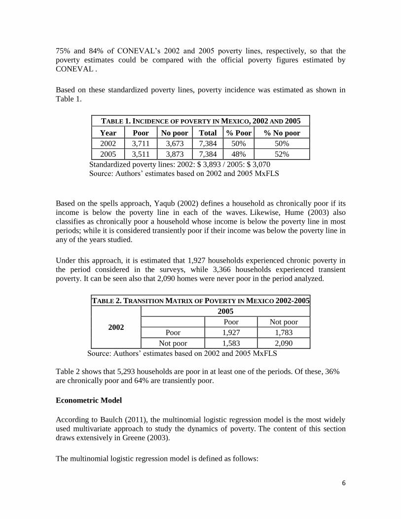
Based on these standardized poverty lines, poverty incidence was estimated as shown in

Table 1.

TABLE 1. INCIDENCE OF POVERTY IN MEXICO, 2002 AND 2005

Year Poor No poor Total % Poor % No poor

2002 3,711 3,673 7,384 50% 50%

2005 3,511 3,873 7,384 48% 52%

Standardized poverty lines: 2002: $ 3,893 / 2005: $ 3,070

Source: Authors’ estimates based on 2002 and 2005 MxFLS

Based on the spells approach, Yaqub (2002) defines a household as chronically poor if its

income is below the poverty line in each of the waves. Likewise, Hume (2003) also

classifies as chronically poor a household whose income is below the poverty line in most

periods; while it is considered transiently poor if their income was below the poverty line in

any of the years studied.

Under this approach, it is estimated that 1,927 households experienced chronic poverty in

the period considered in the surveys, while 3,366 households experienced transient

poverty. It can be seen also that 2,090 homes were never poor in the period analyzed.

TABLE 2. TRANSITION MATRIX OF POVERTY IN MEXICO 2002-2005

2002

2005

Poor Not poor

Poor 1,927 1,783

Not poor 1,583 2,090

Source: Authors’ estimates based on 2002 and 2005 MxFLS

Table 2 shows that 5,293 households are poor in at least one of the periods. Of these, 36%

are chronically poor and 64% are transiently poor.

Econometric Model

According to Baulch (2011), the multinomial logistic regression model is the most widely

used multivariate approach to study the dynamics of poverty. The content of this section

draws extensively in Greene (2003).

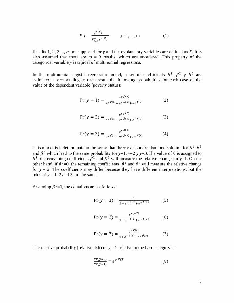
The multinomial logistic regression model is defined as follows:

7

j= 1,…, m (1)

Results 1, 2, 3,..., m are supposed for y and the explanatory variables are defined as X. It is

also assumed that there are m = 3 results, which are unordered. This property of the

categorical variable y is typical of multinomial regressions.

In the multinomial logistic regression model, a set of coefficients , y are

estimated, corresponding to each result the following probabilities for each case of the

value of the dependent variable (poverty status):

(2)

(3)

(4)

This model is indeterminate in the sense that there exists more than one solution for ,

and which lead to the same probability for y=1, y=2 y y=3. If a value of 0 is assigned to

, the remaining coefficients and will measure the relative change for y=1. On the

other hand, if =0, the remaining coefficients and will measure the relative change

for y = 2. The coefficients may differ because they have different interpretations, but the

odds of y = 1, 2 and 3 are the same.

Assuming =0, the equations are as follows:

(5)

(6)

(7)

The relative probability (relative risk) of y = 2 relative to the base category is:

= (8)

8

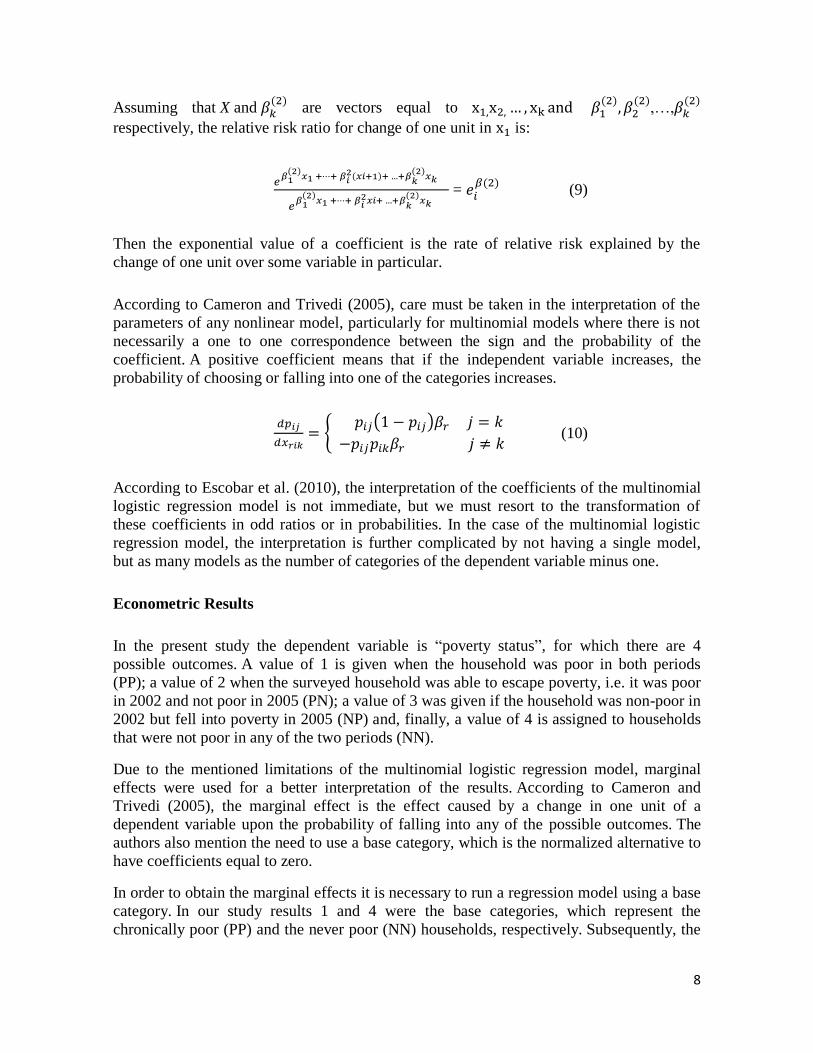
Assuming that X and

are vectors equal to

,…,

respectively, the relative risk ratio for change of one unit in is:

=

(9)

Then the exponential value of a coefficient is the rate of relative risk explained by the

change of one unit over some variable in particular.

According to Cameron and Trivedi (2005), care must be taken in the interpretation of the

parameters of any nonlinear model, particularly for multinomial models where there is not

necessarily a one to one correspondence between the sign and the probability of the

coefficient. A positive coefficient means that if the independent variable increases, the

probability of choosing or falling into one of the categories increases.

(10)

According to Escobar et al. (2010), the interpretation of the coefficients of the multinomial

logistic regression model is not immediate, but we must resort to the transformation of

these coefficients in odd ratios or in probabilities. In the case of the multinomial logistic

regression model, the interpretation is further complicated by not having a single model,

but as many models as the number of categories of the dependent variable minus one.

Econometric Results

In the present study the dependent variable is “poverty status”, for which there are 4

possible outcomes. A value of 1 is given when the household was poor in both periods

(PP); a value of 2 when the surveyed household was able to escape poverty, i.e. it was poor

in 2002 and not poor in 2005 (PN); a value of 3 was given if the household was non-poor in

2002 but fell into poverty in 2005 (NP) and, finally, a value of 4 is assigned to households

that were not poor in any of the two periods (NN).

Due to the mentioned limitations of the multinomial logistic regression model, marginal

effects were used for a better interpretation of the results. According to Cameron and

Trivedi (2005), the marginal effect is the effect caused by a change in one unit of a

dependent variable upon the probability of falling into any of the possible outcomes. The

authors also mention the need to use a base category, which is the normalized alternative to

have coefficients equal to zero.

In order to obtain the marginal effects it is necessary to run a regression model using a base

category. In our study results 1 and 4 were the base categories, which represent the

chronically poor (PP) and the never poor (NN) households, respectively. Subsequently, the

9

marginal effects of the four possible outcomes of the dependent variable (PP, NP, NP and

NN) were obtained for each of the base categories (PP and NN).

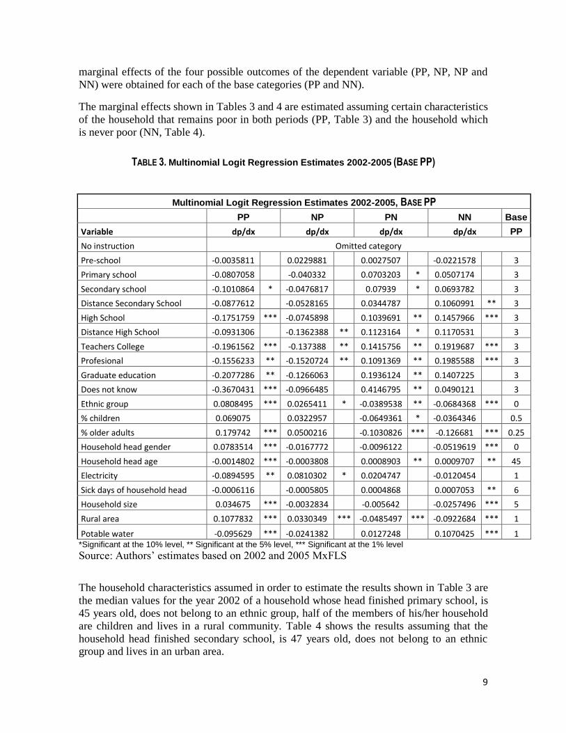
The marginal effects shown in Tables 3 and 4 are estimated assuming certain characteristics

of the household that remains poor in both periods (PP, Table 3) and the household which

is never poor (NN, Table 4).

TABLE 3. Multinomial Logit Regression Estimates 2002-2005 (BASE PP)

Multinomial Logit Regression Estimates 2002-2005, BASE PP

PP NP PN NN Base

Variable dp/dx dp/dx dp/dx dp/dx PP

No instruction Omitted category

Pre-school -0.0035811 0.0229881 0.0027507 -0.0221578 3

Primary school -0.0807058 -0.040332 0.0703203 * 0.0507174 3

Secondary school -0.1010864 * -0.0476817 0.07939 * 0.0693782 3

Distance Secondary School -0.0877612 -0.0528165 0.0344787 0.1060991 ** 3

High School -0.1751759 *** -0.0745898 0.1039691 ** 0.1457966 *** 3

Distance High School -0.0931306 -0.1362388 ** 0.1123164 * 0.1170531 3

Teachers College -0.1961562 *** -0.137388 ** 0.1415756 ** 0.1919687 *** 3

Profesional -0.1556233 ** -0.1520724 ** 0.1091369 ** 0.1985588 *** 3

Graduate education -0.2077286 ** -0.1266063 0.1936124 ** 0.1407225 3

Does not know -0.3670431 *** -0.0966485 0.4146795 ** 0.0490121 3

Ethnic group 0.0808495 *** 0.0265411 * -0.0389538 ** -0.0684368 *** 0

% children 0.069075 0.0322957 -0.0649361 * -0.0364346 0.5

% older adults 0.179742 *** 0.0500216 -0.1030826 *** -0.126681 *** 0.25

Household head gender 0.0783514 *** -0.0167772 -0.0096122 -0.0519619 *** 0

Household head age -0.0014802 *** -0.0003808 0.0008903 ** 0.0009707 ** 45

Electricity -0.0894595 ** 0.0810302 * 0.0204747 -0.0120454 1

Sick days of household head -0.0006116 -0.0005805 0.0004868 0.0007053 ** 6

Household size 0.034675 *** -0.0032834 -0.005642 -0.0257496 *** 5

Rural area 0.1077832 *** 0.0330349 *** -0.0485497 *** -0.0922684 *** 1

Potable water -0.095629 *** -0.0241382 0.0127248 0.1070425 *** 1 *Significant at the 10% level, ** Significant at the 5% level, *** Significant at the 1% level

Source: Authors’ estimates based on 2002 and 2005 MxFLS

The household characteristics assumed in order to estimate the results shown in Table 3 are

the median values for the year 2002 of a household whose head finished primary school, is

45 years old, does not belong to an ethnic group, half of the members of his/her household

are children and lives in a rural community. Table 4 shows the results assuming that the

household head finished secondary school, is 47 years old, does not belong to an ethnic group and lives in an urban area.

10

TABLE 4. Multinomial Logit Regression Estimates 2002-2005 (BASE NN)

Multinomial Logit Regression Estimates 2002-2005, Base NN

PP NP PN NN Base

Variable dp/dx dp/dx dp/dx dp/dx NN

No instruction Omitted category

Pre-school 0.0009456 0.0257026 0.0061419 -0.0327902 4

Primary school -0.0664179 -0.0571618 0.0690733 0.0545064 4

Secondary school -0.0817375 * -0.068083 0.0745015 0.075319 4

Distance Secondary School -0.0748887 -0.0736858 0.0213068 0.1272677 * 4

High School -0.1328256 *** -0.104985 * 0.0826809 0.1551297 4

Distance High School -0.0831783 -0.1476499 *** 0.1013994 0.1294288 4

Teachers College -0.1480969 *** -0.1594836 *** 0.1101277 0.1974528 ** 4

Profesional -0.1254788 *** -0.168505 *** 0.0806679 0.213316 *** 4

Graduate education -0.1530683 ** -0.1497504 * 0.1679083 * 0.1349104 4

Does not know -0.2361114 *** -0.1347586 0.3719291 * -0.0010592 4

Ethnic group 0.0579865 *** 0.0422561 *** -0.023554 -0.0766887 *** 0

% children 0.0488108 * 0.0427748 -0.0596274 * -0.0319582 0.5

% older adults 0.1268268 *** 0.0835612 *** -0.0757725 -0.1346155 *** 0.33

Household head gender 0.0527044 *** 0.0014042 0.0053983 -0.059507 *** 0

Household head age -0.0010382 *** -0.0006536 0.0006846 0.0010072 * 47

Electricity -0.052059 ** 0.0605217 0.0188346 -0.0272974 1

Sick days of household head -0.0004734 * -0.0006784 *** 0.0003527 0.0007991 ** 7

Household size 0.0237464 *** 0.0045973 0.0014118 -0.0297554 *** 4

Rural area 0.0772209 *** 0.0543128 *** -0.0274496 ** -0.1040841 *** 0

Potable water -0.0697079 *** -0.0458028 *** -0.0143431 0.1298538 *** 1 *Significant at the 10% level, ** Significant at the 5% level, *** Significant at the 1% level

Source: Authors’ estimates based on 2002 and 2005 MxFLS

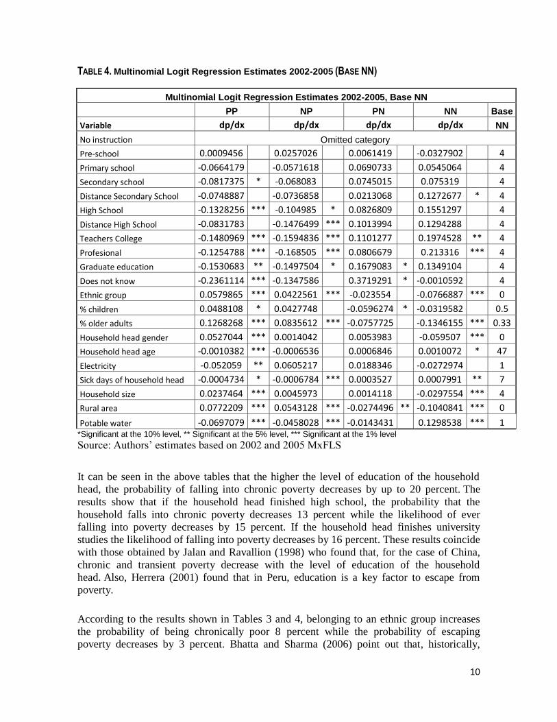
It can be seen in the above tables that the higher the level of education of the household

head, the probability of falling into chronic poverty decreases by up to 20 percent. The

results show that if the household head finished high school, the probability that the

household falls into chronic poverty decreases 13 percent while the likelihood of ever

falling into poverty decreases by 15 percent. If the household head finishes university

studies the likelihood of falling into poverty decreases by 16 percent. These results coincide

with those obtained by Jalan and Ravallion (1998) who found that, for the case of China,

chronic and transient poverty decrease with the level of education of the household

head. Also, Herrera (2001) found that in Peru, education is a key factor to escape from

poverty.

According to the results shown in Tables 3 and 4, belonging to an ethnic group increases

the probability of being chronically poor 8 percent while the probability of escaping

poverty decreases by 3 percent. Bhatta and Sharma (2006) point out that, historically,

11

ethnic groups in many countries have suffered economic, social and political

discrimination, which has been an important factor for these groups to remain in poverty.

We can see in Tables 3 and 4 that if household size increases by one unit, the probability of

falling into chronic poverty increases by 3 percent while the probability of never being poor

decreases by 2 percent. These results coincide with the findings of Quispe (2000), who

found that the probability of being poor increases with family size. However, he notes that

the higher the percentage of household members who are economically active, the lower

the probability of falling into poverty. This is consistent with the results obtained in our

study, which show that there is a direct relationship between the percentage of older adults

and/or children at home and the probability of being poor.

Tables 3 and 4 show that living in a rural area decreases the probability of never falling into

poverty by 2.5 percent, while the probability of being chronically poor increases by 3

percent. Also, having potable water and electricity in the home has an inverse relationship

with chronic poverty. These results agree with those obtained by Baulch and Hoddinott

(2000) for the case of Vietnam, who point out that the lack of electricity and running water

at home decreases the probability of getting out of poverty or never being poor, and

increases the probability of remaining in poverty.

Tables 3 and 4 indicate that if the household is headed by a woman the probability of the

household being chronically poor increases, while the probability of never being poor

decreases. In this respect, Geldstein (1997) notes that the main differences between poor

households headed by women and those headed by men are the low income-generating

capacity of the mother and the lack of economic support from the father. He points out that

when the household head is female, she is often the only person perceiving income among

the household members. On the other hand, when the household head is male it is usually

the case that the household receives income from him but also from his wife.

Conclusions

In the present study, a multinomial logistic regression analysis of the dynamics of poverty

in Mexico was developed. Based on the spells approach to chronic poverty, a transition

matrix was estimated, revealing that, out of a sample of 7,383 households, 1,927

households were chronically poor, 3,366 were transiently poor and 2,090 households were

never poor. Thus, it was estimated that 5,293 households were poor in at least one of the

years of the study period, of which 36% were chronically poor and 64% were transiently

poor.

A multinomial logistic regression analysis was conducted to investigate the effect of

various socioeconomic and demographic variables upon the dynamics of household

poverty. The model showed, among other things, that having a female household head is

positively associated with the likelihood of falling into chronic poverty, and inversely

related to the probability that the household is never poor. It was also found that the greater

12

the level of education of the head of household the lower the probability of falling into

poverty, and the greater the probability that the household can get out of poverty.

Another important finding is that belonging to an ethnic group increases the probability of

falling into poverty. Similarly, an increase in the number of household members makes it

harder for poor households work their way out of poverty. It was found that in general, the

results obtained in this study were similar to the results obtained by other authors for other

countries and they were similar to the results obtained in other studies about poverty

dynamics for the case of Mexico (Garza-Rodriguez et .al, 2010 and Leon (2005)), even

though these last studies used different methodologies.

There are several important policy implications which may be drawn from the results

obtained in this study. First, the government should take into account the large magnitude

of chronic poverty prevailing in the country, as this type of poverty can arguably be more

damaging than transient poverty in the long run. Second, the government body in charge of

measuring poverty in Mexico (CONEVAL), should consider start measuring chronic and

transient poverty in the country. Second, the variables identified in this paper as more

important possible causes or correlates of chronic poverty should be taken into account by

the government in its design and implementation of public policies to alleviate poverty in

the country.

References

Aaberge, R., and M. Mogstad (2007), “On the Definition and Measurement of Chronic

Poverty, Institute for the Study of Labor IZA Discussion Paper No. 2659.

Bane, M., and D. Ellwood (1986). "Slipping into and out of Poverty: The Dynamics of

Spells”, Journal of Human Resources 21 (1), 1-23.

Battha, S. D., & Sharma, S. K. (2006). “The determinants and consequences of chronic and

transitory poverty in Nepal”. Chronic Poverty Research Centre.

Baulch, B., & Hoddinott, J. (2000). “Economic mobility and poverty dynamics in

developing countries”, Journal of Development Studies, 1-24.

Baulch, B., & Masset, E. (2003), "Do Monetary and Nonmonetary Indicators Tell the Same

Story about Chronic Poverty? A Study of Vietnam in the 1990s”, World Development, 31

(3): 441-53.

Baulch, B. and Vu H.D. (2011), “Poverty Dynamics in Vietnam, 2002 to 2006”, in Baulch, B. (Ed.), Why Poverty Persists: Poverty dynamics in Asia and Africa. Cheltenham, U.K,

Edward Elgar, pp. 219-54.

13

Bernal, P. (2007) "Ahorro, Crédito y Acumulación de Activos de los Hogares Pobres de

México". Cuadernos del Consejo de Desarrollo Social 4.

Cameron, A. C., and P. K. Trivedi ( 2005), Microeconometrics: Methods and Applications.

Cambridge University Press.

Escobar Mercado, Modesto F. B. (2010), Análisis de datos con Stata. Madrid: Centro de

Investigaciones Sociológicas.

Garza-Rodriguez, J., Gonzalez-Martinez, M., Quiroga-Lozano, M., Solis-Santoyo, L., &

Yarto-Weber, G. (2010), “Chronic and transient poverty in Mexico: 2002-2005”,

Economics Bulletin, 3188-3020.

Greene, W. (2003), Econometric Analysis. Prentice Hall .

Herrera, J. (2001), “Poverty Dynamics in Peru, 1997-1999”, DIAL DT/2001/09.

Jalan, J. & Ravallion, M. (1998), “Transient Poverty in Postreform Rural China”, Journal

of Comparative Economics, 338-357.

Jalan, J., & Ravallion, M. (2000), “Is transient poverty different? Evidence from rural

China”, Journal of Development Studies.

Justino, P., Litchfield, J., and H.T. Pham (2008), “Poverty Dynamics during Trade Reform:

Evidence from Rural Vietnam”, Review of Income and Wealth, 54, 166-192.

Lee, Nayoung, Geert Ridder, and John Strauss. 2010, “Estimating Poverty Transition

Matrices with Noisy Data”, Department of Economics. University of Southern California.

Leon, E. (2005). “Dinámica de la Pobreza de los Hogares en México para el Periodo 2001-

2002”, Tesis de Licenciatura, Universidad de las Américas.

Lok-Dessallien, R. (2000), Review of Poverty Concepts and Indicators, UNDP Social

Development and Poverty Elimination Division (SEPED) Series on Poverty Reduction.

McCulloch, N. and B. Baulch (1999), “Distinguishing the Chronically From the Transitory

Poor - Evidence from Pakistan”, Working Paper No. 97, Institute of Development

Studies, University of Sussex, UK.

McKay, Andrew, (2003), “Assessing the extent and nature of chronic poverty in low

income countries: issues and evidence”, World Development, 425-439.

Otero, D. (2011), “Imputación de datos faltantes en un sistema de información sobre

conductas de riesgo”, Maestría en técnicas estadísticas, Universidad de Santiago de

Compostela, Santiago de Compostela.

14

uispe, . E., Instituto Nacional de Estad stica e Inform tica (Peru) Programa

MECOVI-Per . (2000). Carac .

Lima: Instituto Nacional de Estad stica e Inform tica.

Rascon E., and L. ubalcava (2009), “Din mica y caracterización de la pobreza urbana en

México”, Spectron Desarrollo.