Multiview Geometry for Camera Networks

Richard J. Radke

Department of Electrical, Computer, and Systems EngineeringRensselaer Polytechnic Institute

Troy, NY, USA

Abstract

Designing computer vision algorithms for camera networks requires an understand-ing of how images of the same scene from different viewpoints are related. Thischapter introduces the basics of multiview geometry in computer vision, includ-ing image formation and camera matrices, epipolar geometry and the fundamentalmatrix, projective transformations, and N -camera geometry. We also discuss fea-ture detection and matching, and describe basic estimation algorithms for the mostcommon problems that arise in multiview geometry.

Key words: image formation, epipolar geometry, projective transformations,structure from motion, feature detection and matching, camera networksPACS: 42.30.-d, 42.30.Sy, 42.30.Tz, 42.30.Va, 42.79.Pw, 02.40.Dr, 02.60.Pn,07.05.Pj

1 Introduction

Multi-camera networks are emerging as valuable tools for safety and securityapplications in environments as diverse as nursing homes, subway stations,highways, natural disaster sites, and battlefields. While early multi-cameranetworks were contained in lab environments and were fundamentally underthe control of a single processor (e.g., [1]), modern multi-camera networksare composed of many spatially-distributed cameras that may have their ownprocessors or even power sources. To design computer vision algorithms thatmake the best use of these cameras’ data, it is critical to thoroughly under-stand the imaging process of a single camera, and the geometric relationshipsinvolved among pairs or collections of cameras.

Our overall goal in this chapter is to introduce the basic terminology of mul-tiview geometry, as well as to describe best practices for several of the most

Preprint submitted to Elsevier 28 September 2008

common and important estimation problems. We begin in Section 2 by dis-cussing the perspective projection model of image formation and the repre-sentation of image points, scene points, and camera matrices. In Section 3,we introduce the important concept of the epipolar geometry that relates apair of perspective cameras, and its representation by the fundamental ma-trix. Section 4 describes projective transformations, which typically arise incamera networks that observe a common ground plane. In Section 5, we brieflydiscuss algorithms for detecting and matching feature points between images,a prerequisite for many of the estimation algorithms we consider. Section 6discusses the general geometry of N cameras, and its estimation using fac-torization and structure-from-motion techniques. Finally, Section 7 concludesthe chapter with pointers to further print and online resources that go intomore detail on the problems introduced here.

2 Image Formation

In this section, we describe the basic perspective image formation model, whichfor the most part accurately reflects the phenomena observed in images takenby real cameras. Throughout the chapter, we denote scene points by X =(X, Y, Z), image points by u = (x, y), and camera matrices by P .

2.1 Perspective Projection

An idealized “pinhole” camera C is described by:

(1) A center of projection C ∈ R3

(2) A focal length f ∈ R+

(3) An orientation matrix R ∈ SO(3).

The camera’s center and orientation are described with respect to a worldcoordinate system on R3. A point X expressed in the world coordinate systemas X = (Xo, Yo, Zo) can be expressed in the camera coordinate system of C as

X =

XC

YC

ZC

= R

Xo

Yo

Zo

− C . (1)

The purpose of a camera is to capture a two-dimensional image of a three-dimensional scene S, i.e., a collection of points in R3. This image is produced by

2

Camera Coordinates

ImageCoordinates

X

Y Z

X = (XC, YC, ZC)

u = (x, y)

f

x

y

Fig. 1. A pinhole camera uses perspective projection to represent a scene pointX ∈ R3 as an image point u ∈ R2.

perspective projection as follows. Each camera C has an associated image planeP , located in the camera coordinate system at ZC = f . As illustrated in Figure1, the image plane inherits a natural orientation and two-dimensional coordi-nate system from the camera coordinate system’s XY -plane. It is importantto note that the three-dimensional coordinate systems in this derivation areleft-handed. This is a notational convenience, implying that the image planelies between the center of projection and the scene, and that scene points havepositive ZC coordinates.

A scene point X = (XC, YC, ZC) is projected onto the image plane P at thepoint u = (x, y) by the perspective projection equations

x = fXCZC

y = fYCZC. (2)

The image I that is produced is a map from P into some color space. Thecolor of a point is typically a real-valued (grayscale) intensity or a triplet ofRGB or YUV values. While the entire ray of scene points {λ(x, y, f)|λ > 0}is projected to the image coordinate (x, y) by (2), the point on this ray thatgives (x, y) its color in the image I is the one closest to the image plane (i.e.,that point with minimal λ). This point is said to be visible; any scene pointfurther along on the same ray is said to be occluded.

For real cameras, the relationship between the color of image points and thecolor of scene points is more complicated. To simplify matters, we often assumethat scene points have the same color regardless of the viewing angle (this iscalled the Lambertian assumption), and that the color of an image point isthe same as the color of a single corresponding scene point. In practice, thecolors of corresponding image and scene points are different due to a hostof factors in a real imaging system. These include the point spread function,

3

color space, and dynamic range of the camera, as well as non-Lambertian orsemi-transparent objects in the scene. For more detail on the issues involvedin image formation, see [2,3].

2.2 Camera Matrices

Frequently, an image coordinate (x, y) is represented by the homogeneous coor-dinate λ(x, y, 1), where λ 6= 0. The image coordinate of a homogeneous coordi-nate (x, y, z) can be recovered as (x

z, y

z) when z 6= 0. Similarly, any scene point

(X, Y, Z) can be represented in homogeneous coordinates as λ(X, Y, Z, 1),where λ 6= 0. We use the symbol ∼ to denote the equivalence between ahomogeneous coordinate and a non-homogeneous one.

A camera C with parameters (C, f,R) can be represented by a 3×4 matrix PCthat multiplies a scene point expressed as a homogeneous coordinate in R4 toproduce an image point expressed as a homogeneous coordinate in R3. Whenthe scene point is expressed in the world coordinate system, the matrix P isgiven by

PC =

f 0 0

0 f 0

0 0 1

[R | −RC] . (3)

Here, the symbol | denotes the horizontal concatenation of two matrices. Then

PC

X

Y

Z

1

=

f 0 0

0 f 0

0 0 1

[R | −RC]

X

Y

Z

1

=

f 0 0

0 f 0

0 0 1

R

X

Y

Z

− C =

f 0 0

0 f 0

0 0 1

XC

YC

ZC

=

fXC

fYC

ZC

∼

f XCZC

f XCZC

.

4

We often state this relationship succinctly as

u ∼ PX. (4)

2.2.1 Intrinsic and Extrinsic Parameters

We note that the camera matrix can be factored as

P = K R [I | − C]. (5)

The matrix K contains the intrinsic parameters of the camera, while thevariables R and C comprise the extrinsic parameters of the camera, specifyingits position and orientation in the world coordinate system. While the intrinsicparameter matrix K in (3) was just a diagonal matrix containing the focallength, a more general camera can be constructed using a K matrix of theform

K =

mx

my

1

f s/mx px

f py

1

. (6)

In addition to the focal length of the camera f , this intrinsic parameter ma-trix includes mx and my, the number of pixels per x and y unit of imagecoordinates, respectively; (px, py), the coordinates of the principal point of theimage, and s, the skew (deviation from rectangularity) of the pixels. For high-quality cameras, the pixels are usually square, the skew is typically 0, and theprincipal point can often be approximated by the image origin.

A general camera matrix has 11 degrees of freedom (since it is only defined upto a scale factor). The camera center and the rotation matrix each account for3 degrees of freedom, leaving 5 degrees of freedom for the intrinsic parameters.

2.2.2 Extracting Camera Parameters from P

Often, we begin with an estimate of a 3 × 4 camera matrix P and want toextract the intrinsic and extrinsic parameters from it. The homogeneous coor-dinates of the camera center C can be simply extracted as the right-hand nullvector of P (i.e., a vector satisfying PC = 0). If we denote the left 3× 3 blockof P as M , then we can factor M = KR where K is upper triangular and Ris orthogonal using a modified version of the QR decomposition [4]. Enforcing

5

that K has positive values on its diagonal should remove any ambiguity aboutthe factorization.

2.2.3 More General Cameras

While the perspective model of projection generally matches the image for-mation process of a real camera, an affine model of projection is sometimesmore computationally appealing. While less mathematically accurate, such anapproximation may be acceptable in cases where the depth of scene points isfairly uniform, or the field of view is fairly narrow. Common choices for linearmodels include orthographic projection, in which the camera matrix has theform

P =

1 0 0 0

0 1 0 0

0 0 0 1

R t

0 1

, (7)

or weak perspective projection, in which the camera matrix has the form

P =

αx 0 0 0

0 αy 0 0

0 0 0 1

R t

0 1

. (8)

Finally, we note that real cameras frequently exhibit radial lens distortion,which can be modeled by

xy

= L(√x2 + y2)

xy

, (9)

where (x, y) is the result of applying the perspective model (4), and L(·) isa function of the radial distance from the image center, often modeled asa fourth-degree polynomial. The parameters of the distortion function aretypically measured off-line using a calibration grid [5].

2.3 Estimating the Camera Matrix

The P matrix for a given camera is typically estimated based on a set ofmatched correspondences between image points uj ∈ R2 and scene points

6

Xj with known coordinates in R3. That is, the goal is to select the matrixP ∈ R3×4 that best matches a given set of point mappings:

{Xj 7→ uj, j = 1, . . . , N}. (10)

Each correspondence (uj,Xj) produces two independent linear equations inthe elements of P . Thus, the equations for all the data points can be collectedinto a linear system Ap = 0, where A is an 2N ×12 matrix involving the data,and p = (p11, . . . , p34)T is the vector of unknowns. Since the camera matrix isunique up to scale, we must fix some scaling (say, ||p||2 = 1) to ensure thatAp cannot become arbitrarily small.

The least-squares minimization problem is then

min ‖Ap‖2 s.t. pTp = 1. (11)

The solution to this problem is well known; the minimizer is the eigenvec-tor p ∈ R12 of ATA corresponding to the minimal eigenvalue, which can becomputed via the singular value decomposition. This eigenvector is then re-assembled into a 3 × 4 matrix P , which can be factored into intrinsic andextrinsic parameters as described above.

To maintain numerical stability, it is critical to normalize the data beforesolving the estimation problem. That is, each of the sets {uj} and {Xj} shouldbe translated to have zero mean, and then isotropically scaled so that theaverage distance to the origin is

√2 for the image points and

√3 for the

scene points. These translations and scalings can be represented by similaritytransform matrices T and U that act on the homogeneous coordinates of theuj and Xj. After the camera matrix for the normalized points P has beenestimated, the estimate of the camera matrix in the original coordinates isgiven by

P = T−1PU. (12)

Several more advanced algorithms for camera matrix estimation (also calledresectioning) are discussed in Hartley and Zisserman [6], typically requiringiterative, nonlinear optimization.

When the datasets contain outliers (i.e., incorrect point correspondences in-consistent with the underlying projection model), it is necessary to detectand reject them during the estimation process. Frequently, the robust estima-tion framework called RANSAC [7] is employed for this purpose. RANSAC isbased on randomly selecting a large number of data subsets, each containingthe minimal number of correspondences that make the estimation problemsolvable. An estimate of the outlier probability is used to select a number

7

of subsets to guarantee that at least one of the minimal subsets has a highprobability of containing all inliers.

The point correspondences required for camera matrix estimation are typi-cally generated using images of a calibration grid resembling a high-contrastcheckerboard. Bouguet authored a widely-disseminated camera calibrationtoolbox in Matlab that only requires the user to print and acquire severalimages of such a calibration grid [8].

3 Two-Camera Geometry

Next, we discuss the image relationships resulting from the same static scenebeing imaged by two cameras C and C ′, as illustrated in Figure 2. These couldbe two physically separate cameras, or a single moving camera at differentpoints in time. Let the scene coordinates of a point X in the C coordinatesystem be (X, Y, Z), and in the C ′ coordinate system be (X ′, Y ′, Z ′). We denotethe corresponding image coordinates of X in P and P ′ by u = (x, y) andu′ = (x′, y′), respectively. The points u and u′ are said to be correspondingpoints, and the pair (u, u′) is called a point correspondence.

Y

X = (X, Y, Z) = (X’, Y’, Z’)

X

Z

f

u = (x, y)

Y’

-X’

Z’

f ’

u’ = (x’, y’)

Fig. 2. The rigid motion of a camera introduces a change of coordinates, resultingin different image coordinates for the same scene point X.

Assuming standard values for the intrinsic parameters, the scene point Xis projected onto the image points u and u′ via the perspective projectionequations (2):

x = fX

Zy = f

Y

Z(13)

x′ = f ′X ′

Z ′y′ = f ′

Y ′

Z ′. (14)

8

Here f and f ′ are the focal lengths of C and C ′, respectively. We assumethat the two cameras are related by a rigid motion, which means that the C ′coordinate system can be expressed as a rotation R of the C coordinate systemfollowed by a translation [tX tY tZ ]T . That is,

X ′

Y ′

Z ′

= R

X

Y

Z

+

tX

tY

tZ

. (15)

In terms of the parameters of the cameras, R = R′R−1 and t = R′(C − C ′).Alternately, we can write R as

R =

cosα cos γ + sinα sin β sin γ cos β sin γ − sinα cos γ + cosα sin β sin γ

− cosα sin γ + sinα sin β cos γ cos β cos γ sinα sin γ + cosα sin β cos γ

sinα cos β − sin β cosα cos β

,(16)

where α, β and γ are rotation angles around theX, Y , and Z axes, respectively,of the C coordinate system.

By substituting equation (15) into the perspective projection equations (2),we obtain a relationship between the two sets of image coordinates:

x′ = f ′X ′

Z ′=r11

f ′

fx+ r12

f ′

fy + r13f

′ + tXf ′

Zr31

fx+ r32

fy + r33 + tZ

Z

(17)

y′ = f ′Y ′

Z ′=r21

f ′

fx+ r22

f ′

fy + r23f

′ + tY f ′

Zr31

fx+ r32

fy + r33 + tZ

Z

. (18)

Here the rij are the elements of the rotation matrix given in (16). In Section4 we will consider some special cases of (17)-(18).

3.1 The Epipolar Geometry and its Estimation

We now introduce the fundamental matrix, which encapsulates an importantconstraint on point correspondences between two images of the same scene.For each generic pair of cameras (C, C ′), there exists a matrix F of rank two

9

such that for all correspondences (u, u′) = ((x, y), (x′, y′)) ∈ P × P ′,

x′

y′

1

T

F

x

y

1

= 0. (19)

The fundamental matrix is unique up to scale provided that there exists noquadric surface Q containing the line C C ′ and every point in the scene S [9].

Given the fundamental matrix F for a camera pair (C, C ′), we obtain a con-straint on the possible locations of point correspondences between the associ-ated image pair (I, I ′).

Π

CC’

X

uu’

e e’

P P

’

‘

Fig. 3. The relationship between two images of the same scene is encapsulated bythe epipolar geometry. For any scene point X, we construct the plane Π containingX and the two camera centers. This plane intersects the image planes at the twoepipolar lines ` and `′. Any image point on ` in I must have its correspondenceon `′ in I ′. The projections of the camera centers C ′ and C onto I and I ′ are theepipoles e and e′, respectively.

The epipolar line corresponding to a point u ∈ P is the set of points:

10

`u =

u′ = (x′, y′)T ∈ P ′

∣∣∣∣∣∣∣∣u′

1

T

F

u1

= 0

. (20)

If u is the image of scene point X in P , the image u′ of X in P ′ is constrainedto lie on the epipolar line `u. Epipolar lines for points in P ′ can be definedaccordingly. Hence, epipolar lines exist in conjugate pairs (`, `′), such that thematch to a point u ∈ ` must lie on `′, and vice versa. Conjugate epipolar linesare generated by intersecting any plane Π containing the baseline C C ′ withthe pair of image planes (P ,P ′) (see Figure 3). For a more thorough reviewof epipolar geometry, the reader is referred to [10].

The epipoles e ∈ P and e′ ∈ P ′ are the projections of the camera centersC ′ and C onto P and P ′, respectively. It can be seen from Figure 3 that theepipolar lines in each image all intersect at the epipole. In fact, the homoge-neous coordinates of the epipoles e and e′ are the right and left eigenvectorsof F , respectively, corresponding to the eigenvalue 0.

Since corresponding points must appear on conjugate epipolar lines, they forman important constraint that can be exploited while searching for featurematches, as illustrated in Figure 4.

Fig. 4. Image pair, with sample epipolar lines. Corresponding points must occuralong conjugate epipolar lines; for example, consider the goalie’s head or the frontcorner of the goal area.

3.2 Relating the Fundamental Matrix to the Camera Matrices

The fundamental matrix can easily be constructed from the two camera ma-trices. If we assume that

P = K [I | 0] P ′ = K ′ [R | t], (21)

11

then the fundamental matrix is given by

F = K ′−T [t]×RK−1 = K ′−TR[RT t]×K

−1, (22)

where [t]× is the skew-symmetric matrix defined by

[t]× =

0 −t3 t2

t3 0 −t1−t2 t1 0

. (23)

In the form of (22), we can see that F is rank-2 since [t]× is rank-2. Since F isonly unique up to scale, the fundamental matrix has 7 degrees of freedom. Theleft and right epipoles can also be expressed in terms of the camera matricesas follows:

e = KRT t e′ = K ′t. (24)

From the above, the fundamental matrix for a pair of cameras is clearly uniqueup to scale. However, there are 4 degrees of freedom in extracting P and P ′

from a given F . This ambiguity arises since the camera matrix pairs (P, P ′)and (PH,P ′H) have the same fundamental matrix for any 4× 4 nonsingularmatrix H (e.g., the same rigid motion applied to both cameras). The familyof (P, P ′) corresponding to a given F is described by:

P = [I | 0] P ′ = [[e′]×F + e′vT | λe′], (25)

where v ∈ R3 is an arbitrary vector and λ is a non-zero scalar.

In cases where the intrinsic parameter matrix K of the camera is known (e.g.,estimated offline using a calibration grid), then the homogeneous image coor-dinates can be transformed using

u = K−1u u′ = K ′−1u′. (26)

The camera matrices become

P = [I | 0] P ′ = [R | t], (27)

and the fundamental matrix is now called the essential matrix. The advantage

12

of the essential matrix is that its factorization in terms of the extrinsic cameraparameters

E = [t]×R = R[RT t]× (28)

is unique up to four possible solutions, the correct of which can be determinedby requiring that all projected points lie in front of both cameras [6].

3.3 Estimating the Fundamental Matrix

The fundamental matrix is typically estimated based on a set of matchedpoint correspondences (see Section 5). That is, the goal is to select the matrixF ∈ R3×3 that best matches a given set of point mappings:

{uj 7→ u′j ∈ R2, j = 1, . . . , N} (29)

It is natural to try to minimize a least-squares cost functional such as

J(F ) =N∑

j=1

u′j1

T

F

uj

1

(30)

over the class of admissible fundamental matrices. We recall that F must haverank two (see Section 3.2). Furthermore, the fundamental matrix is unique upto scale, so we must fix some scaling (say, ‖F‖ = 1 for some appropriate norm)to ensure that J cannot become arbitrarily small. Hence, the class of admissibleestimates has only seven degrees of freedom. Constrained minimizations ofthis type are problematic due to the difficulty in parameterizing the class ofadmissible F . Faugeras and Luong [11–13] proposed some solutions in thisregard and analyzed various cost functionals for the estimation problem.

A standard approach to estimating the fundamental matrix was proposed byHartley [14]. Ignoring the rank-two constraint for the moment, we minimize(30) over the class {F ∈ R3×3 | ‖F‖F = 1}, where ‖·‖F is the Frobenius norm.

Each correspondence (uj, u′j) produces a linear equation in the elements of F :

xjx′jf11 + xjy

′jf21 + xjf31 + yjx

′jf21 + yjy

′jf22 + yjf23 + x′jf31 + y′jf32 + f33 = 0

The equations in all the data points can be collected into a linear system Af =

13

0, where A is an N×9 matrix involving the data, and f = (f11, f21, f31, f12, f22,f32, f13, f23, f33)T is the vector of unknowns. The least-squares minimizationproblem is then

min ‖Af‖2 s.t. fTf = 1 (31)

As in the resectioning estimation problem in Section 2.3, the minimizer is theeigenvector f ∈ R9 of ATA corresponding to the minimal eigenvalue, whichcan be computed via the singular value decomposition. This eigenvector isthen reassembled into a 3× 3 matrix F .

To account for the rank-two constraint, we replace the full-rank estimate Fby F ∗, the minimizer of

min ‖F − F ∗‖F s.t. rank(F ∗) = 2. (32)

Given the singular value decomposition F = UDV T , where D = diag(r, s, t)with r > s > t, the solution to (32) is

F ∗ = UDV T , (33)

where D = diag(r, s, 0).

As in Section 2.3, to maintain numerical stability, it is critical to normalizethe data before solving the estimation problem. Each of the sets {uj} and{u′j} should be translated to have zero mean, and then isotropically scaled so

that the average distance to the origin is√

2. These translations and scalingscan be represented by 3× 3 matrices T and T ′ that act on the homogeneouscoordinates of the uj and u′j. After the fundamental matrix for the normalizedpoints has been estimated, the estimate of the fundamental matrix in theoriginal coordinates is given by

F = T ′T F ∗T. (34)

The overall estimation process is called the normalized eight-point algorithm.Several more advanced algorithms for fundamental matrix estimation are dis-cussed in Hartley and Zisserman [6], typically requiring iterative, nonlinearoptimization. As before, outliers (i.e., incorrect point correspondences incon-sistent with the underlying epipolar geometry) are often detected and rejectedusing RANSAC.

14

4 Projective Transformations

The fundamental matrix constrains the possible locations of correspondingpoints: they must occur along conjugate epipolar lines. However, there aretwo special situations in which the fundamental matrix for an image pair isundefined, and instead point correspondences between the images are relatedby an explicit one-to-one mapping.

Let us reconsider equations (17) and (18) that relate the image coordinatesof a point seen by two cameras C and C ′. For this relationship to define atransformation that globally relates the image coordinates, for every scenepoint (X, Y, Z) we would require that the dependence on the world coordinateZ disappears, i.e. that

tXZ

= a1Xx+ a2Xy + bX (35)

tYZ

= a1Y x+ a2Y y + bY (36)

tZZ

= a1Zx+ a2Zy + bZ (37)

for some set of a’s and b’s. These conditions are satisfied when either:

(1) tX = tY = tZ = 0 or(2) k1X + k2Y + k3Z = 1.

In the first case, corresponding to a camera whose optical center undergoesno translation, we obtain

x′=r11

f ′

fx+ r12

f ′

fy + r13f

′

r31

fx+ r32

fy + r33

y′=r21

f ′

fx+ r22

f ′

fy + r23f

′

r31

fx+ r32

fy + r33

.

An example of three such images composed into the same frame of referencewith appropriate projective transformations is illustrated in Figure 5.

In the second case, corresponding to a planar scene, (17) and (18) become:

15

Fig. 5. Images from a non-translating camera, composed into the same frame ofreference by appropriate projective transformations.

x′=(r11

f ′

f+ tXf

′k1)x+ (r12f ′

f+ tXf

′k2)y + (r13f′ + tXf

′k3)

( r31

f+ tZk1)x+ ( r32

f+ tZk2)y + (r33 + tZk3)

(38)

y′=(r21

f ′

f+ tY f

′k1)x+ (r22f ′

f+ tY f

′k2)y + (r23f′ + tY f

′k3)

( r31

f+ tZk1)x+ ( r32

f+ tZk2)y + (r33 + tZk3)

An example of a pair of images of a planar surface, registered by an appropriateprojective transformation, is illustrated in Figure 6.

Fig. 6. Images of a planar scene, composed into the same frame of reference byappropriate projective transformations.

In either case, the transformation is of the form

16

x′=a11x+ a12y + b1

c1x+ c2y + d(39)

y′=a21x+ a22y + b2

c1x+ c2y + d, (40)

which can be written in homogeneous coordinates as

u′ = Hu (41)

for a nonsingular 3 × 3 matrix H defined up to scale. This relationship iscalled a projective transformation (sometimes also known as a collineation ora homography). When c1 = c2 = 0, the transformation is known as an affinetransformation.

Projective transformations between images are induced by common cameraconfigurations such as surveillance cameras that view a common ground planeor a panning and tilting camera mounted on a tripod. In the next section, wediscuss how to estimate projective transformations relating an image pair.

We note that technically, affine transformations are induced by the motionof a perspective camera only under quite restrictive conditions. The imageplanes must both be parallel to the XY -plane. Furthermore, either the trans-lation vector t must be identically 0, or Z must be constant for all points inthe scene, i.e., the scene is a planar surface parallel to the image planes Pand P ′. However, the affine assumption is often made when the scene is farfrom the camera (Z is large) and the rotation angles α and β are very small.This assumption has the advantage that the affine parameters can be easilyestimated, usually in closed form.

4.1 Estimating Projective Transformations

The easiest approach to estimating a projective transformation from pointcorrespondences is called the direct linear transform (DLT). If the point cor-respondence {uj 7→ u′j} corresponds to a projective transformation, then thehomogeneous coordinates u′j and Huj are vectors in the same direction, i.e.,

u′j ×Huj = 0. (42)

Since (42) gives 2 independent linear equations in the 9 unknowns of H, Npoint correspondences give rise to a 2N × 9 linear system

17

Ah = 0, (43)

where A is a 2N×9 matrix involving the data, and h = (a11, a12, a22, a22, b1, b2,c1, c2, d)T is the vector of unknowns. We solve the problem in exactly the sameway as (31) using the singular value decomposition (i.e., the solution h is thesingular vector of A corresponding to the smallest singular value).

When the element d is expected to be far from 0, an alternate approach is tonormalize d = 1, in which case the N point correspondences induce a systemof 2N equations in the remaining 8 unknowns, which can be solved as a linearleast-squares problem.

As with the fundamental matrix estimation problem, more accurate estimatesof the projective transformation parameters can be obtained by the iterativeminimization of a nonlinear cost function, such as the symmetric transfer errorgiven by

N∑i=1

||u′i −Hui||22 + ||ui −H−1u′i||22. (44)

The reader is referred to Hartley and Zisserman [6] for more details. We notethat an excellent turnkey approach to estimating projective transformationsfor real images is given by the Generalized Dual-Bootstrap ICP algorithmproposed by Yang et al. [15].

4.2 Rectifying Projective Transformations

We close this section by mentioning a special class of projective transforma-tions called rectifying projective transformations that often simplify computervision problems involving point matching along conjugate epipolar lines.

Since epipolar lines are generally not aligned with one of the coordinate axesof an image, or are even parallel, the implementation of algorithms that workwith epipolar lines can be complicated. To this end, it is common to apply atechnique called rectification to an image pair before processing, so that theepipolar lines are parallel and horizontal.

An associated image plane pair (P ,P ′) is said to be rectified when the funda-

18

mental matrix for (P ,P ′) is the skew-symmetric matrix

F∗ =

0 0 0

0 0 1

0 −1 0

. (45)

In homogeneous coordinates, the epipoles corresponding to F∗ are e0 = e1 =[1 0 0]T , which means the epipolar lines are horizontal and parallel. Fur-thermore, expanding the fundamental matrix equation for a correspondence((x, y)T , (x′, y′)T ) ∈ P × P ′ gives

x′

y′

1

T

F∗

x

y

1

= 0, (46)

which is equivalent to y′ − y = 0. This implies that not only are the epipolarlines in a rectified image pair horizontal, they are aligned, so that the linesy = λ in P and y′ = λ in P ′ are conjugate epipolar lines.

FHG e

PP^

e’

P‘ P^

‘

Fig. 7. Rectifying projective transformations G and H transform correspondingepipolar lines to be horizontal with the same y-value.

A pair of projective transformations (G,H) is called rectifying for an associ-ated image plane pair (P ,P ′) with fundamental matrix F if

H−TFG−1 = F∗. (47)

By the above definition, if the projective transformations G and H are appliedto P and P ′ to produce warped image planes P0 and P1, respectively, then(P0, P1) is a rectified pair (Figure 7).

The rectifying condition (47) can be expressed as 9 equations in the 16 un-knowns of the two projective transformations G and H, leading to 7 degrees offreedom in the choice of a rectifying pair. Seitz [16] and Hartley [17] describedmethods for deriving rectifying projective transformations from an estimate ofthe fundamental matrix relating an image pair. Isgro and Trucco [18] observed

19

that rectifying transformations can be estimated without explicitly estimatingthe fundamental matrix as an intermediate step.

5 Feature Detection and Matching

As indicated in the previous sections, many algorithms for multiview geom-etry parameter estimation problems require a set of image correspondencesas input, i.e., regions of pixels representing scene points that can be reliably,unambiguously matched in other images of the same scene.

Many indicators of pixel regions that constitute “good” features have beenproposed, including line contours, corners, and junctions. A classical algorithmfor detecting and matching “good” point features was proposed by Shi andTomasi [19], described as follows:

(1) Compute the gradients gx(x, y) and gy(x, y) for I. That is,

gx(x, y) = I(x, y)− I(x− 1, y)

gy(x, y) = I(x, y)− I(x, y − 1).

(2) For every N ×N block of pixels Γ,(a) Compute the covariance matrix

B =

∑(x,y)∈Γ g

2x(x, y)

∑(x,y)∈Γ gxgy(x, y)∑

(x,y)∈Γ gxgy(x, y)∑

(x,y)∈Γ g2y(x, y)

.(b) Compute the eigenvalues of B, λ1 and λ2.(c) If λ1 and λ2 are both greater than some threshold τ , add Γ to the

list of features.(3) For every block of pixels Γ in the list of features, find the N ×N block of

pixels in I ′ that has the highest normalized cross-correlation, and add thepoint correspondence to the feature list if the correlation is sufficientlyhigh.

A recent focus in the computer vision community has been on different types of“invariant” detectors that select image regions that can be robustly matchedeven between images where the camera perspectives or zooms are quite dif-ferent. An early approach was the Harris corner detector [20], which uses thesame matrix B as the Shi-Tomasi algorithm, but instead of computing theeigenvalues of B, the quantity

ρ = det(B)− κ · trace2(Z) (48)

20

is computed, with κ in a recommended range of 0.04-0.15. Blocks with localpositive maxima of ρ are selected as features. Mikolajczyk and Schmid [21]later extended Harris corners to a multi-scale setting.

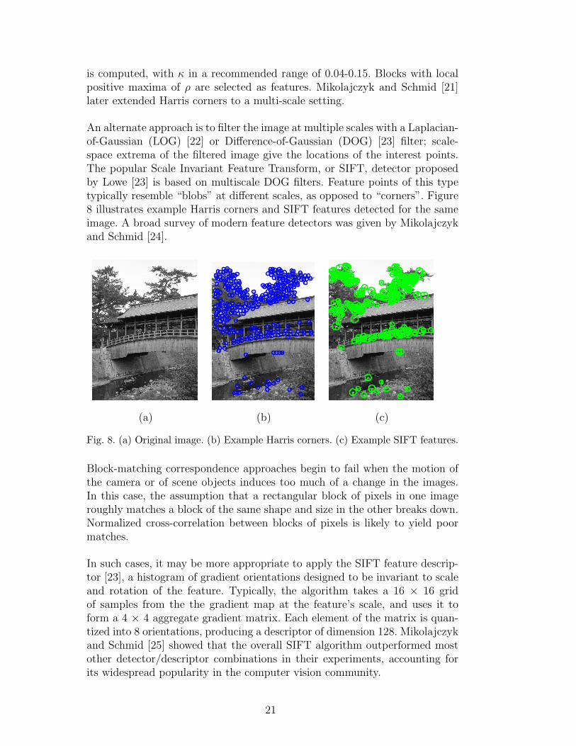
An alternate approach is to filter the image at multiple scales with a Laplacian-of-Gaussian (LOG) [22] or Difference-of-Gaussian (DOG) [23] filter; scale-space extrema of the filtered image give the locations of the interest points.The popular Scale Invariant Feature Transform, or SIFT, detector proposedby Lowe [23] is based on multiscale DOG filters. Feature points of this typetypically resemble “blobs” at different scales, as opposed to “corners”. Figure8 illustrates example Harris corners and SIFT features detected for the sameimage. A broad survey of modern feature detectors was given by Mikolajczykand Schmid [24].

(a) (b) (c)

Fig. 8. (a) Original image. (b) Example Harris corners. (c) Example SIFT features.

Block-matching correspondence approaches begin to fail when the motion ofthe camera or of scene objects induces too much of a change in the images.In this case, the assumption that a rectangular block of pixels in one imageroughly matches a block of the same shape and size in the other breaks down.Normalized cross-correlation between blocks of pixels is likely to yield poormatches.

In such cases, it may be more appropriate to apply the SIFT feature descrip-tor [23], a histogram of gradient orientations designed to be invariant to scaleand rotation of the feature. Typically, the algorithm takes a 16 × 16 gridof samples from the the gradient map at the feature’s scale, and uses it toform a 4 × 4 aggregate gradient matrix. Each element of the matrix is quan-tized into 8 orientations, producing a descriptor of dimension 128. Mikolajczykand Schmid [25] showed that the overall SIFT algorithm outperformed mostother detector/descriptor combinations in their experiments, accounting forits widespread popularity in the computer vision community.

21

6 Multi-Camera Geometry

We now proceed to the relationships between M > 2 cameras that observethe same scene. While there is an entity called the trifocal tensor [26] relatingthree cameras’ views that plays an analogous role to the fundamental matrixfor two views, here we concentrate on the geometry of M general cameras.

We assume a camera network that contains M perspective cameras, each de-scribed by a 3 × 4 matrix Pi. Each camera images some subset of a set ofN scene points {X1,X2, . . . ,XN} ∈ R3. We define an indicator function χij

where χij = 1 if camera i images scene point j. The projection of Xj onto Pi

is given by uij ∈ R2, denoted

uij ∼ PiXj. (49)

The main problem in multi-camera geometry is called structure from motion(SFM). That is, given only the observed image projections {uij}, we want toestimate the corresponding camera matrices Pi and scene points Xj. As wediscuss in the next sections, this process typically proceeds in stages to find agood initial estimate, which is followed by a nonlinear optimization algorithmcalled bundle adjustment.

We note that SFM is closely related to a problem in the robotics communitycalled Simultaneous Localization and Mapping (SLAM) [27], in which mobilerobots must estimate their locations from sensor data as they move through ascene. SFM also forms the fundamental core of commercial software packagessuch as Boujou or SynthEyes for the problems of “matchmoving” or cameratracking, which are used to insert digital effects into Hollywood movies.

6.1 Affine Reconstruction

Many initialization methods for the SFM problem involve a factorization ap-proach. The first such approach was proposed by Tomasi and Kanade [28] andapplies only to affine cameras (we generalize it to perspective cameras in thenext section).

For an affine camera, the projection equations take the form

uij = AiXj + ti (50)

for Ai ∈ R2×3 and ti ∈ R2. If we assume that each camera images all of the

22

scene points, then a natural formulation of the affine SFM problem is:

min{Ai,ti,Xj}

M∑i=1

N∑j=1

‖uij − (AiXj + ti)‖2 (51)

If we assume that the Xj are centered at 0, taking the derivative with respectto ti reveals that the minimizer

ti =1

N

N∑i=1

uij. (52)

Hence, we recenter the image measurements by

uij ←− uij −1

N

N∑i=1

uij (53)

and are faced with solving

min{Ai,Xj}

M∑i=1

N∑j=1

‖uij − AiXj‖2. (54)

Tomasi and Kanade’s key observation was that if all of the image coordinatesare collected into a measurement matrix defined by

W =

u11 u12 · · · u1N

u21 u22 · · · u2N

......

. . ....

uM1 uM2 · · · uMN

, (55)

then in the ideal (noiseless) case, this matrix factors as

W =

A1

A2

...

AM

[X1 X2 · · · XN ], (56)

revealing that the 2M×N measurement matrix is ideally rank-3. They showedthat solving (54) is equivalent to finding the best rank-3 approximation to W

23

in the Frobenius norm, which can easily be accomplished with the singularvalue decomposition. The solution is unique up to an affine transformationof the world coordinate system, and optimal in the sense of maximum likeli-hood estimation if the noise in the image projections is isotropic, zero-meani.i.d. Gaussian.

6.2 Projective Reconstruction

Unfortunately, for the perspective projection model that more accurately re-flects the way real cameras image the world, factorization is not as easy. Wecan form a similar measurement matrix W and factorize it as follows:

W =

λ11u11 λ12u12 · · · λ1Nu1N

λ21u21 λ22u22 · · · λ2Nu2N

......

. . ....

λM1uM1 λm2um2 · · · λMNuMN

=

P1

P2

...

PM

(

X1 X2 · · · XN

). (57)

Here, both the uij and Xj are represented in homogeneous coordinates. There-fore, the measurement matrix is of dimension 3M ×N and is ideally rank-4.However, since the scale factors (also called projective depths) λij multiplyingeach projection are different, these must also be estimated.

Sturm and Triggs [29,30] suggested a factorization method that recovers theprojective depths as well as the structure and motion parameters from themeasurement matrix. They used relationships between fundamental matricesand epipolar lines in order to obtain an initial estimate for the projectivedepths λij (an alternate approach is to simply initialize all λij = 1). Once theprojective depths are fixed, the rows and columns of the measurement matrixare rescaled, and the camera matrices and scene point positions are recoveredfrom the best rank-4 approximation to W obtained using the singular valuedecomposition. Given estimates of the camera matrices and scene points, thescene points can then be reprojected to obtain new estimates of the projectivedepths, and the process iterated until the parameter estimates converge.

24

6.3 Metric Reconstruction

There is substantial ambiguity in a projective reconstruction as obtainedabove, since

P1

P2

...

PM

[X1 X2 · · · XN ] =

P1H

P2H...

PMH

[H−1X1 H

−1X2 · · · H−1XN ] (58)

for any 4 × 4 nonsingular matrix H. This means that while some geometricproperties of the reconstructed configuration will be correct compared to thetruth (e.g., the order of 3D points lying along a straight line), others willnot (e.g., the angles between lines/planes or the relative lengths of line seg-ments). In order to make the reconstruction useful (i.e., to recover the correctconfiguration up to an unknown rotation, translation, and scale), we need toestimate the matrix H that turns the projective factorization into a metricfactorization, so that

PiH = KiRTi [I | − Ci] . (59)

and Ki is in the correct form (e.g., we may force it to be diagonal). Thisprocess is also called auto-calibration.

The auto-calibration process depends fundamentally on several properties ofprojective geometry that are subtle and complex. We only give a brief overviewhere; see [31,32,6] for more details.

If we let mx = my = 1 in (6), then the form of a camera’s intrinsic parametermatrix is

K =

αx s x

0 αy y

0 0 1

. (60)

We define a quantity called the dual image of the absolute conic (DIAC) as

ω∗ = KKT =

α2

x + s2 + x2 sαy + xy x

sαy + xy α2y + y2 y

x y 1

. (61)

25

If we put constraints on the camera’s internal parameters, these correspondto constraints on the DIAC. For example, if we require that the pixels havezero skew and that the principal point is at the origin, then

ω∗ =

α2

x 0 0

0 α2y 0

0 0 1

, (62)

and we have introduced 3 constraints on the entries of the DIAC:

ω∗12 = ω∗13 = ω∗23 = 0. (63)

If we further constrain that the pixels must be square, then we have a fourthconstraint that ω∗11 = ω∗22.

The DIAC is related to a second important quantity called the absolute dualquadric, denoted Q∗∞. This is a special 4 × 4 symmetric rank-3 matrix thatrepresents an imaginary surface in the scene that is fixed under similaritytransformations. That is, points on Q∗∞ map to other points on Q∗∞ if a rota-tion, translation, and/or uniform scaling is applied to the scene coordinates.

The DIAC (which is different for each camera) and Q∗∞ (which is independentof the cameras) are connected by the important equation

ω∗i = P iQ∗∞PiT . (64)

That is, the two quantities are related through the camera matrices P i. There-fore, each constraint we impose on each ω∗i (e.g., each of (63)) imposes a linearconstraint on the 10 homogeneous parameters of Q∗∞, in terms of the cameramatrices P i. Given enough camera matrices, we can thus solve a linear least-squares problem for the entries of Q∗∞.

Once Q∗∞ has been estimated from the {P i} resulting from projective factor-ization, the correct H matrix in (59) that brings about a metric reconstructionis extracted using the relationship

Q∗∞ = Hdiag(1, 1, 1, 0)HT . (65)

The resulting reconstruction is related to the true camera/scene configura-tion by an unknown similarity transform that cannot be estimated withoutadditional information about the scene.

26

We conclude this section by noting that there exist critical motion sequencesfor which auto-calibration is not fully possible [33], including pure translationor pure rotation of a camera, orbital motion around a fixed point, or motionconfined to a plane.

6.4 Bundle Adjustment

After a good initial metric factorization is obtained, the final step is to per-form bundle adjustment, i.e., the iterative optimization of the nonlinear costfunction

M∑i=1

N∑j=1

χij(uij − PiXj)T Σ−1

ij (uij − PiXj). (66)

Here, Σij is the 2×2 covariance matrix associated with the noise in the imagepoint uij. The quantity inside the sum is called the Mahalanobis distancebetween the observed image point and its projection based on the estimatedcamera/scene parameters.

The optimization is typically accomplished with the Levenberg-Marquardtalgorithm [34], specifically an implementation that exploits the sparse blockstructure of the normal equations characteristic of SFM problems (since eachscene point is typically observed by only a few cameras) [35].

Parameterization of the minimization problem, especially of the cameras, isa critical issue. If we assume that the skew, aspect ratio, and principal pointof each camera are known prior to deployment, then each camera should berepresented by 7 parameters: 1 for the focal length, 3 for the translation vector,and 3 for the rotation matrix parameters.

Rotation matrices are often minimally parameterized by 3 parameters (v1, v2, v3)using the axis-angle parameterization. If we think of v as a vector in R3, thenthe rotation matrix R corresponding to v is a rotation through the angle ‖v‖about the axis v, computed by

R = cos ‖v‖I + sinc‖v‖[v]× +1− cos ‖v‖‖v‖2

vvT . (67)

Extracting the v corresponding to a given R is accomplished as follows. Thedirection of the rotation axis v is the eigenvector of R corresponding to theeigenvalue 1. The angle φ that defines ‖v‖ is obtained from the two-argumentarctangent function using

27

2 cos(φ) = trace(R)− 1 (68)

2 sin(φ) = (R32 −R23, R13 −R31, R21 −R12)Tv. (69)

Other parameterizations of rotation matrices and rigid motions were discussedby Chirikjian and Kyatkin [36].

Finally, it is important to remember that the set of cameras and scene pointscan only be estimated up to an unknown rotation, translation, and scale ofthe world coordinates, so it is common to fix the extrinsic parameters of thefirst camera as

P1 = K1 [I | 0]. (70)

In general, any over-parameterization of the problem or ambiguity in the re-constructions creates a problem called gauge freedom [37], which can lead toslower convergence and computational problems. Therefore, it is important tostrive for minimal parameterizations of SFM problems.

7 Further Resources

Multiple view geometry is a rich and complex area of study, and this chapteronly gives an introduction to the main geometric relationships and estimationalgorithms. The best and most comprehensive reference on epipolar geometry,structure from motion, and camera calibration is Multiple View Geometry inComputer Vision, by Richard Hartley and Andrew Zisserman [6], which isessential reading for further study of the material discussed here.

The collected volume Vision Algorithms: Theory and Practice (Proceedingsof the International Workshop on Vision Algorithms), edited by Bill Triggs,Andrew Zisserman, and Richard Szeliski [38] contains an excellent, detailedarticle on bundle adjustment in addition to important papers on gauges andparameter uncertainty.

Finally, An Invitation to 3D Vision: From Images to Geometric Models, by YiMa, Stefano Soatto, Jana Kosecka, and Shankar Sastry [39], is an excellent ref-erence that includes a chapter giving a beginning-to-end recipe for structure-from-motion. The companion website includes Matlab code for most of thealgorithms described in this chapter [40].

We conclude by noting that the concepts discussed in this chapter are nowviewed as fairly classical in the computer vision community. However, there isstill much interesting research to be done in extending and applying computervision algorithms in the context of distributed camera networks; several such

28

cutting-edge algorithms are discussed in this book. The key challenges are that

(1) A very large number of widely-distributed cameras may be involved in arealistic camera network. The set-up is fundamentally different in termsof scale and spatial extent compared to typical multi-camera researchundertaken in a research lab setting.

(2) The information from all cameras is unlikely to be available at a pow-erful, central processor, an underlying assumption of the multi-cameracalibration algorithms discussed in Section 6. Instead, each camera maybe attached to a power- and computation-constrained local processor thatis unable to execute complex algorithms, and an antenna that is unableto transmit information across long distances.

These considerations argue for distributed algorithms that operate indepen-dently at each camera node, exchanging information between local neighborsto obtain solutions that approximate the best performance of a centralizedalgorithm. For example, we recently presented a distributed algorithm for thecalibration of a multi-camera network that was designed with these consider-ations in mind [41]. We refer the reader to our recent survey on distributedcomputer vision algorithms [42] for more information.

References

[1] T. Kanade, P. Rander, P. Narayanan, Virtualized reality: Constructing virtualworlds from real scenes, IEEE Multimedia, Immersive Telepresence 4 (1) (1997)34–47.

[2] D. Forsyth, J. Ponce, Computer Vision: A Modern Approach, Prentice Hall,2003.

[3] P. Shirley, Fundamentals of Computer Graphics, A.K. Peters, 2002.

[4] G. Strang, Linear Algebra and its Applications, Harcourt Brace Jovanovich,1988.

[5] B. Prescott, G. F. McLean, Line-based correction of radial lens distortion,Graphical Models and Image Processing 59 (1) (1997) 39–47.

[6] R. Hartley, A. Zisserman, Multiple View Geometry in Computer Vision,Cambridge University Press, 2000.

[7] M. A. Fischler, R. C. Bolles, Random sample consensus: A paradigm formodel fitting with applications to image analysis and automated cartography,Communications of the ACM 24 (1981) 381–395.

[8] J.-Y. Bouguet, Camera calibration toolbox for matlab, in:http://www.vision.caltech.edu/bouguetj/calib doc/, 2008.

29

[9] S. Maybank, The angular velocity associated with the optical flowfield arisingfrom motion through a rigid environment, Proc. Royal Soc. London A 401(1985) 317–326.

[10] Z. Zhang, Determining the epipolar geometry and its uncertainty - a review,The International Journal of Computer Vision 27 (2) (1998) 161–195.

[11] O. Faugeras, Three-Dimensional Computer Vision: A Geometric Viewpoint,MIT Press, 1993.

[12] O. Faugeras, Q.-T. Luong, T. Papadopoulo, The Geometry of Multiple Images:The Laws That Govern the Formation of Multiple Images of a Scene and Someof Their Applications, MIT Press, 2001.

[13] Q.-T. Luong, O. Faugeras, The fundamental matrix: Theory, algorithms, andstability analysis, International Journal of Computer Vision 17 (1) (1996) 43–76.

[14] R. Hartley, In defence of the 8-point algorithm, in: Proc. ICCV ’95, 1995, pp.1064–1070.

[15] G. Yang, C. V. Stewart, M. Sofka, C.-L. Tsai, Registration of challenging imagepairs: Initialization, estimation, and decision, IEEE Transactions on PatternAnalysis and Machine Intelligence 29 (11) (2007) 1973–1989.

[16] S. Seitz, Image-based transformation of viewpoint and scene appearance, Ph.D.thesis, University of Wisconsin at Madison (1997).

[17] R. Hartley, Theory and practice of projective rectification, International Journalof Computer Vision 35 (2) (1999) 115–127.

[18] F. Isgro, E. Trucco, Projective rectification without epipolar geometry, in: Proc.CVPR ’99, 1999.

[19] J. Shi, C. Tomasi, Good features to track, in: IEEE Computer SocietyConference on Computer Vision and Pattern Recognition, 1994, pp. 593–600.

[20] C. Harris, M. Stephens, A combined corner and edge detector, in: Proceedingsof the Fourth Alvey Vision Conference, Manchester, UK, 1988, pp. 147–151.

[21] K. Mikolajczyk, C. Schmid, Indexing based on scale invariant interest points, in:Procedings of the IEEE International Conference on Computer Vision (ICCV),Vancouver, Canada, 2001, pp. 525–531.

[22] T. Lindeberg, Detecting salient blob-like image structures and their scales with ascale-space primal sketch: a method for focus-of-attention, International Journalof Computer Vision 11 (3) (1994) 283–318.

[23] D. G. Lowe, Distinctive image features from scale-invariant keypoints,International Journal of Computer Vision 60 (2) (2004) 91–110.

[24] K. Mikolajczyk, C. Schmid, Scale and affine invariant interest point detectors,International Journal of Computer Vision 60 (1) (2004) 63–86.

30

[25] K. Mikolajczyk, C. Schmid, A performance evaluation of local descriptors, IEEETransactions on Pattern Analysis and Machine Intelligence 27 (10) (2005) 1615–1630.

[26] A. Shashua, M. Werman, On the trilinear tensor of three perspective views andits underlying geometry, in: Proc. of the International Conference on ComputerVision (ICCV), 1995.

[27] S. Thrun, W. Burgard, D. Fox, Probabilistic Robotics: Intelligent Robotics andAutonomous Agents, MIT Press, 2005.

[28] C. Tomasi, T. Kanade, Shape and Motion from Image Streams: A FactorizationMethod Part 2. Detection and Trcking of Point Features, Tech. Rep. CMU-CS-91-132, Carnegie Mellon University (April 1991).

[29] P. Sturm, B. Triggs, A factorization based algorithm for multi-image projectivestructure and motion, in: Proceedings of the 4th European Conference onComputer Vision (ECCV ’96), 1996, pp. 709–720.

[30] B. Triggs, Factorization methods for projective structure and motion, in:Proceedings of IEEE Conference on Computer Vision and Pattern Recognition(CVPR ’96), IEEE Comput. Soc. Press, San Francisco, CA, USA, 1996, pp.845–51.

[31] M. Pollefeys, R. Koch, L. J. Van Gool, Self-calibration and metric reconstructionin spite of varying and unknown internal camera parameters, in: Proceedingsof the IEEE International Conference on Computer Vision (ICCV), 1998, pp.90–95.

[32] M. Pollefeys, F. Verbiest, L. J. V. Gool, Surviving dominant planes inuncalibrated structure and motion recovery, in: Proceedings of the 7th EuropeanConference on Computer Vision-Part II (ECCV ’02), Springer-Verlag, London,UK, 2002, pp. 837–851.

[33] P. Sturm, Critical motion sequences for monocular self-calibration anduncalibrated Euclidean reconstruction, in: Proceedings of the IEEEInternational Conference on Computer Vision and Pattern Recognition, 1997,pp. 1100–1105.

[34] J. Dennis, Jr., R. Schnabel, Numerical Methods for Unconstrained Optimizationand Nonlinear Equations, SIAM Press, 1996.

[35] B. Triggs, P. McLauchlan, R. Hartley, A. Fitzgibbon, Bundle adjustment –A modern synthesis, in: W. Triggs, A. Zisserman, R. Szeliski (Eds.), VisionAlgorithms: Theory and Practice, LNCS, Springer Verlag, 2000, pp. 298–375.

[36] G. Chirikjian, A. Kyatkin, Engineering applications of noncommutativeharmonic analysis with emphasis on rotation and motion groups, CRC Press,2001.

[37] K. Kanatani, D. D. Morris, Gauges and gauge transformations for uncertaintydescription of geometric structure with indeterminacy, IEEE Transactions onInformation Theory 47 (5) (2001) 2017–2028.

31

[38] B. Triggs, A. Zisserman, R. Szeliski (Eds.), Vision Algorithms: Theory andPractice (Proceedings of the International Workshop on Vision AlgorithmsCorfu, Greece, September 21-22, 1999), Springer, 2000.

[39] Y. Ma, S. Soatto, J. Kosecka, S. S. Sastry, An Invitation to 3-D Vision, Springer,2004.

[40] Y. Ma, S. Soatto, J. Kosecka, S. S. Sastry, An invitation to 3-D vision, in:http://vision.ucla.edu/MASKS/.

[41] D. Devarajan, Z. Cheng, R. Radke, Calibrating distributed camera networks,Proceedings of the IEEE (Special Issue on Distributed Smart Cameras) 96 (10).

[42] R. Radke, A survey of distributed computer vision algorithms, in:H. Nakashima, J. Augusto, H. Aghajan (Eds.), Handbook of AmbientIntelligence and Smart Environments, Springer, 2008.

32