1

Multivariate Statistics

ESM 206, 5/17/05

2

WHAT IS MULTIVARIATE STATISTICS?

• A collection of techniques to help us understand patterns in and make predictions with large datasets with many variables

• Ordination: find a (hopefully small) number of composite variables that capture most of the variability among data points

• Cluster Analysis: discover natural groupings of similar data points

• Discriminant Analysis: find a (hopefully small) number of composite variables that can be used to predict the levels of a categorical dependent variable

• Canonical Correlation Analysis: find relationships between two groups of variables– “Dependent variable” is multivariate

3

WHAT CAN MULTIVARIATE STATISTICS DO?

• Reflect more accurately the true multidimensional nature of environmental systems

• Provide a way to handle large datasets with large numbers of variables by summarizing the redundancy

• Provide rules for combining variables in an “optimal” way

• Provide a means of detecting and quantifying truly multivariate patterns that arise out of correlational structure of the variable set

• Provide a means of exploring complex data sets for patterns and relationships from which hypotheses can be generated and subsequently tested experimentally

4

DISTINGUISHING ECOLOGICAL NICHES OF 3 SPECIES

5

6

7

ORDINATION

• Simplify the interpretation of complex data by organizing sampling entities along independent gradients or factors defined by combinations of interrelated variables

• Uncover a more fundamental set of factors that account for the major patterns across all of the original variables

• If a few major gradients explain much of the variability in data, then data can be interpreted with respect to these gradients without loss of information

8

PRINCIPAL COMPONENTS ANALYSIS (PCA)

• Most commonly used ordination technique

• Given P correlated variables, extract P principal components– Linear combinations of the variables

– Uncorrelated with one another

– First PC is direction through data cloud that captures the most variance in data

– Second PC is direction perpendicular to first that captures the most remaining variance

– Etc.

• Assumptions of PCA:1. Data are multivariate normal

2. Data are independent

3. Observed variables depend linearly on underlying factors

• May need to transform data to satisfy these

• Unless variables are all measured on same scale, use correlations rather than covariances– Gives equal weight to variability in

all variables

9

EXAMPLE: CHEMICAL SOLUBILITY

• 72 chemical compounds tested for solubility in each of 6 solvents– Solubility measure on log scale

• Strong (but not perfect) correlations among the 6 solvents

• Can we use fewer than 6 variables to characterize each chemical?

-0.5

0.5

1.5

2.5

-1.00.01.0

2.5

-1

1

3

-2

0

2

-3

-1

1

3

-4

-2

0

2

1-Octanol

-0.5 .5 1.5 2.5

Ether

-1.0.0 1.0 2.5

Chloroform

-1 0 1 2 3 4

Benzene

-2-1 0 1 2 3

CarbonTetrachloride

-3 -1 0 1 2 3

Hexane

-4 -2 0 1 2 3

Scatterplot Matrix

Multivariate

10

Eigenvalue

Percent

Cum Percent

1-Octanol

Ether

Chloroform

Benzene

Carbon Tetrachloride

Hexane

Eigenvectors

4.7850

79.7502

79.7502

0.37441

0.34834

0.41940

0.44561

0.43102

0.42217

0.9452

15.7538

95.5040

0.55987

0.64314

-0.29864

-0.14756

-0.29736

-0.27117

0.1399

2.3309

97.8348

-0.11070

0.11973

-0.64850

-0.21904

0.18487

0.68608

0.0611

1.0182

98.8530

-0.65842

0.62764

0.30599

-0.09455

-0.24135

0.10831

0.0471

0.7850

99.6380

0.31660

-0.20890

0.43061

-0.49849

-0.45965

0.45926

0.0217

0.3620

100.0000

0.01874

0.11456

0.18793

-0.68865

0.64968

-0.23426

Principal Components: on Correlations

Principal Components / Factor Analysis

Multivariate

SOLUBILITY PCA• Eigenvalue indicates how much of

the variability in data is explained by the PC – Magnitude depends on number of

variables (and variances if done with covariance matrix)

– Instead look at percents

• Eigenvector gives coefficients of linear relationship of PC to each variable– NOTE: some software scales the

eignvectors differently

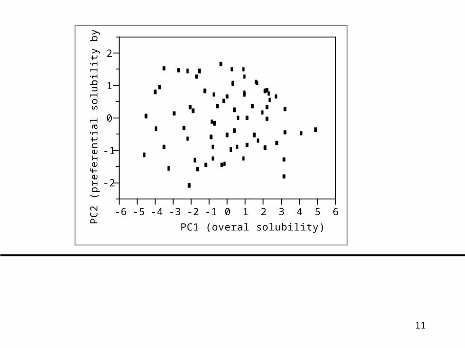
• Interpretation: PC1 is axis of overall increasing solubility

• PC2 is axis of differential solubility in 1-Ocatanol & Ether vs. other 4 solvents

PC1 0.37 0.35 0.42 0.45

0.43 0.42

O E C B

CT H

11

-2

-1

0

1

2

PC

2 (p

refe

rent

ial s

olub

ility

by 1

-Oct

anol

& E

ther

)

-6 -5 -4 -3 -2 -1 0 1 2 3 4 5 6

PC1 (overal solubility)

12

CHARACTRISTICS OF ORDINATION• Organizes sampling entities (e.g.,

species, sites, observations) along continuous environmental gradients

• Assesses relationships within single set of variables; doesn’t define relationship between a set of independent variables and one or more dependent variables– However, PC’s can be used as

independent variables in a regression

• Reduces dimensionality of multivariate data set by condensing large # of original variables into smaller set of new composite variables with minimal loss of information

• Summarizes data redundancy by placing similar entities in proximity in ordination space

• Defines new composite variables (e.g., principal components) as weighted linear combinations of the original variables

• Eliminates noise from a multivariate data set by recovering patterns in first few composite dimensions and deferring noise to subsequent axes

13

OTHER ORDINATION TECHNIQUES

• Polar Ordination (PO)• Factor Analysis (FA)

– This is often used as a generic term meaning “ordination” in social sciences

• Nonmetric Multidimensional Scaling (NMMDS)– Relaxes normality and linearity

assumptions by using ranks

• Correspondence Analysis (CA)– Allows data (e.g., species

abundance) to take on peak values at intermediate levels of the gradient

– Also called Reciprocal Averaging

• Detrended Correspondence Analysis (DCA)– Deals particularly well with

nonlinear relationships

• Canonical Correspondence Analysis (CCA)– Like CA, but ordination of variables

of interest (e.g., species abundance) is constrained to depend linearly on other variables (e.g., environmental characteristics) measured at same sites

14

FURTHER READING

• McGarigal, K., S. Cushman, and S. Stafford. 2000. Multivariate Statistics for Wildlife and Ecology Research (Springer-Verlag, New York).

• Gotelli, H.J., and A.M. Ellison. 2004. A Primer of Ecological Statistics (Sinauer, Sunderland, MA); Chapter 12.

• Spicer, J. 2005. Making Sense of Multivariate Data Analysis (Sage Press, Thousand Oaks).