Multivariate significance testing and model calibration under uncertainty

Available online at www.sciencedirect.com

www.elsevier.com/locate/cma

Comput. Methods Appl. Mech. Engrg. 197 (2008) 2467–2479

Multivariate significance testing and model calibrationunder uncertainty

John McFarland, Sankaran Mahadevan *

Vanderbilt University, VU Station B #351831, 2301 Vanderbilt Place, Nashville, TN 37235, United States

Received 6 May 2007; received in revised form 25 May 2007; accepted 25 May 2007Available online 23 December 2007

Abstract

The importance of modeling and simulation in the scientific community has drawn interest towards methods for assessing the accu-racy and uncertainty associated with such models. This paper addresses the validation and calibration of computer simulations using thethermal challenge problem developed at Sandia National Laboratories for illustration. The objectives of the challenge problem are to usehypothetical experimental data to validate a given model, and then to use the model to make predictions in an untested domain. Withregards to assessing the accuracy of the given model (validation), we illustrate the use of Hotelling’s T2 statistic for multivariate signif-icance testing, with emphasis on the formulation and interpretation of such an analysis for validation assessment. In order to use themodel for prediction, we next employ the Bayesian calibration method introduced by Kennedy and O’Hagan. Towards this end, we dis-cuss how inherent variability can be reconciled with ‘‘lack-of-knowledge” and other uncertainties, and we illustrate a procedure thatallows probability distribution characterization uncertainty to be included in the overall uncertainty analysis of the Bayesian calibrationprocess.� 2007 Elsevier B.V. All rights reserved.

Keywords: Model validation; Multivariate statistics; Significance testing; Hypothesis testing; Calibration; Uncertainty

1. Introduction

This paper addresses the thermal validation challengeproblem [1], which is a hypothetical problem that presentsthe analyst with several pieces of validation data and a cor-responding mathematical model. The first objective putforth by the challenge problem is to use material character-ization data to estimate a probabilistic model for the phys-ical properties which are inputs to the mathematical model.The second and third objectives involve assessing the mod-el’s accuracy based on available experimental data (modelvalidation). The final objective is to use the model to pre-dict whether or not a specified regulatory requirement willbe met.

0045-7825/$ - see front matter � 2007 Elsevier B.V. All rights reserved.

doi:10.1016/j.cma.2007.05.030

* Corresponding author. Tel.: +1 615 322 3040; fax: +1 615 322 3365.E-mail addresses: [email protected] (J. McFarland),

[email protected] (S. Mahadevan).

Section 2 addresses the first objective, and how the mate-rial property data (which clearly indicate temperaturedependence) will be used in such a way that the given model(which does not allow for such temperature dependence) isnot modified. Section 3 addresses the second and thirdobjectives and discusses how a quantitative statistical signif-icance test (Hotelling’s T2) can be used to assess the valida-tion data, given that the measured and predicted responsequantities are not only multivariate (temperature is mea-sured at 10 instances in time for the ‘‘ensemble” experi-ments), but also nearly linearly dependent in time. Thefourth objective is addressed in Section 4, which illustratesthe use of model calibration under uncertainty for enhanc-ing the predictive capability of the given model. Finally, theresults and conclusions are discussed in Section 5.

The purpose of the model validation process is to com-pare simulator predictions with observed experimentaloutcomes to assess the sufficiency of the accuracy of aparticular simulation model. A significant amount of the

mailto:[email protected]

mailto:[email protected]

2468 J. McFarland, S. Mahadevan / Comput. Methods Appl. Mech. Engrg. 197 (2008) 2467–2479

previous work has dealt with outlining general frameworksand methodologies [2–5]. Although there has been a grow-ing interest in the development of quantitative measures forassessing validity, there is still much more work to be done.

Ref. [2] describes several desired features of a validationmetric, and they also propose several quantitative metricswhich showcase these criteria. Among other things, theyargue that the metric should depend on the number ofexperimental replications of a measurement quantity, thusreflecting a ‘‘level of confidence”. Ref. [3] also states that ‘‘auseful validation metric should only measure the agreementbetween the computational results and the experimentaldata”.

Statistical significance testing (or hypothesis testing)seems like a natural tool for model validation for severalreasons. First, significance tests directly address the ques-tion of whether or not available data provide significantevidence against a particular hypothesis, taking rigorousaccount of sample size. Issues such as the ‘‘level of confi-dence” can also be quantified using other considerations,such as the ‘‘power” of the test. Recent work that has con-sidered the use of hypothesis testing for model validationincludes [6–11], and the Bayesian perspective on hypothesistesting has been explored as well [12,13]. Ref. [14] even dis-cusses a method for incorporating Bayesian hypothesistesting with risk considerations for the purpose of decisionmaking.

In addition to validation, the second thrust of the chal-lenge problem is to use the given model for predictions, andgiven the availability of experimental data, this logicallyentails a calibration process. Previous work dealing withthe calibration of computer simulations is somewhat lim-ited. Ref.’s [15,16] give overviews, with particular interestin methods which make attempts to account for uncer-tainty. One of the most straightforward approaches is topose the calibration problem in terms of nonlinear regres-sion analysis. The problem is then attacked using standardoptimization techniques to minimize, for example, the sumof the squared errors between the predictions and observa-tions. Ref. [17] illustrates the use of such a method toobtain point estimates and various types of confidenceintervals for a groundwater flow model.

Other methods which have been proposed include theGeneralized Likelihood Uncertainty Estimation (GLUE)procedure [18], which is somewhat Bayesian in that itattempts to characterize a predictive response distributionby weighting random parameter samples by their likeli-hoods. However, the GLUE method does not assume aparticular distributional form for the errors. Methods hav-ing their foundation in system identification and beingrelated to the Kalman filter have also been proposed formodel calibration, and are particularly suited for situationsin which new data become available over time [19,20].

One of the milestone papers for model calibration isKennedy and O’Hagan [21]. Not only does this formula-tion treat the computational simulation as a black-box,replacing it by a Gaussian process surrogate, but it also

claims to account for all of the uncertainties and variabili-ties which may be present. Towards this end, the calibra-tion problem is formulated using a Bayesian framework,and both multiplicative and additive ‘‘discrepancy” termsare allowed to account for any deviations of the predictionsfrom the experimental data which are not taken up in thesimulation parameters. Further, the additive discrepancyterm is formulated as a Gaussian process indexed by thescenario variables (boundary conditions, initial conditions,etc. . .) which describe the system being modeled. In thisregard, their formulation is particularly powerful for casesin which experimental data are available at multiple differ-ent scenarios, and predictions of interest are characterizedby extrapolations (or interpolations) in this scenario space.Implementation of their complete framework is quitedemanding and requires extensive use of numerical integra-tion techniques such as quadrature or Markov ChainMonte Carlo integration.

The remainder of this paper addresses each of the fourobjectives outlined in the thermal challenge problem [1].First, Section 2 discusses how the material characterizationdata are used to estimate probability distributions for twoof the model input parameters (objective 1). Next, Section3 addresses the validation aspects of the challenge problemusing multivariate significance testing to compare themodel predictions to the experimental observations (objec-tives 2 and 3). The use of principal components analysis forhandling singular covariance is discussed in Section 3.1.1,and methods for characterizing the power of the tests arecovered in Section 3.1.2. Finally, Section 4 illustrates howthe given model is used together with the available experi-mental data to make predictions regarding whether or notthe devices will meet the given regulatory requirements(objective 4). This is done by first using the Bayesian cali-bration framework developed by Kennedy and O’Haganto calibrate the model using the experimental data. Conclu-sions are discussed in Section 5.

2. Use of material data and mathematical model

The first challenge problem objective is to use data fromthe ‘‘material characterization experiments” to characterizea probabilistic model for the material properties k and qC,which are inputs to the heat-transfer model. Several chal-lenges arise at this stage, as it is quickly apparent that thereis a relationship between the thermal conductivity, k, andtemperature. However, the inclusion of a temperature-dependent material model requires modification of thegiven analytical heat-transfer solution (e.g., implementationof an iterative solution scheme), and doing so is decidedlyinconsistent with the purpose of the challenge problem’svalidation activities, which are to assess the accuracy ofand make predictions with an inherently ‘‘flawed” model(one that ignores the temperature-dependence of the mate-rial properties).

This analysis refrains completely from adjusting theheat-transfer model to account for temperature dependency

J. McFarland, S. Mahadevan / Comput. Methods Appl. Mech. Engrg. 197 (2008) 2467–2479 2469

of the thermal conductivity. A ‘‘run” of the simulator is thusperformed by providing one value each for k and qC toobtain temperature predictions for each time instance ofinterest. Not only is this consistent with the ‘‘code verifica-tion” discussed in the challenge problem description [1], butby treating the model as a ‘‘black box”, the methods pre-sented are more generally applicable.

The procedure used here is to characterize each of thematerial properties using (independent) probability distri-butions. The variance of qC is estimated directly fromthe data, whereas the variance of k is estimated using a sim-ple linear regression model of the material characterizationdata as a function of temperature. This allows us to isolatethe variance related to specimen-to-specimen variability. Ineach case, the mean values are estimated directly from thedata. Further, we employ the normal distribution modelfor both properties. The normal distribution is used partlyfor parsimony: a more complex probabilistic model may beless interpretable and also may be at risk of over-character-izing the actual property variation. But we also choose thenormal distribution because the data do not strongly sug-gest otherwise. Specifically, we apply two well-known testsfor normality, the Lilliefors test [22] and the Shapiro–Wilktest [23], to the data for qC and the regression residuals fork. The results are included in Table 1, suggesting that in nocase do the data provide strong evidence against theassumption of normality.

Additionally, for the validation exercises, we are con-cerned with getting accurate estimates of the material prop-erty means that will allow for relevant predictions at eachexperimental configuration. This consideration leads us touse a censoring scheme when estimating the property distri-butions for the validation exercises. Only property mea-surements corresponding to temperatures less than orequal to 500 �C are used for analysis of the ‘‘ensemble val-idation” data, and only property measurements made attemperatures less than or equal to 750 �C are used for anal-ysis of the ‘‘accreditation” data.

The resulting statistics of the material properties aregiven in Table 1 (for the high data level).

Table 1Statistics of material property data (high data level) and p-values fornormality tests

Data set n Property Mean Standarddeviation

Shapirotest (p-value)

Lillieforstest (p-value)

T 6 500 �C 18 k (W/m �C)

0.0569 0.00435 0.48 0.24

qC (J/m3 �C)

3.92E5 3.69E4 0.79 0.92

T 6 750 �C 24 k 0.0599 0.00398 0.70 0.31qC 3.94E5 3.76E4 0.45 0.84

All T 30 k 0.0628 0.00470 0.51 0.49qC 3.94E5 3.63E4 0.44 0.58

3. Model validation

This section addresses the challenge problem objectiveswhich deal with making assessments of the accuracy ofthe given mathematical model. The approach below illus-trates one method for computing quantitative validationmeasures, based on statistical significance testing (a.k.a.hypothesis testing). Of particular interest is the fact thatthe system response quantity under consideration (temper-ature) is measured at multiple instances in time. In order totake proper account of the dependencies which arise whena quantity is measured over time, multivariate statisticaltechniques are employed for significance testing. This willinclude the use of principal components analysis to enableinference given that the temperature values are nearly line-arly dependent.

The actual heat-transfer model provided in the thermalchallenge problem is computationally trivial to evaluate,making it straightforward to obtain the model’s output dis-tribution using simple Monte Carlo simulation (recall thattwo of the model’s input parameters are random variables).However, in many cases, the model may be costly and/ortime-consuming to evaluate, making it necessary to useapproximation methods to estimate the model’s output dis-tribution. In such cases, efficient approximation methodssuch as the stochastic response surface method (SRSM)[24] can be used to estimate the model’s output distribu-tion, in which case the validation analysis described inthe remainder of this section would be carried out in thesame manner.

3.1. Significance testing: Hotelling’s T2 statistic

The use of significance testing (or hypothesis testing) isnot widespread in the validation community, but themethod nevertheless provides several features which mightbe deemed useful for a validation metric. Significance test-ing addresses in a rigorous sense whether or not the dataoffer significant evidence against a certain hypothesis, tak-ing into account such factors as sample size and variability.Concepts such as the probabilities of type I and II errorsalso provide constructive ways of thinking about how thedecision maker might approach the validation problem(see, for example, [14,25]). Alternatively, the use of confi-dence intervals or regions is structurally analogous to thatof significance testing, and is sometimes used instead forease of interpretation (see [26] for an example of the useof confidence regions for multivariate validation inference).

With regards to significance testing, in the univariatecase (considering one response measure only), the relevantvalidation question might be whether or not the data sug-gest that the location of the experimental observations issignificantly different than that of the model output.Assuming that either the model being validated is ‘‘fast”(i.e., inexpensive to evaluate), or that we have an appropri-ate approximation to the distribution of the model output,we can formally test whether the data (the experimental


observations) offer significant evidence against the nullhypothesis H0: l = l0, where l is the (unknown) mean ofthe population of experimental data, and l0 is the (known)mean of the model output. In most cases this hypothesis isanalyzed using the well-known Student’s t-test, which isbased on the statistic

t ¼ �x� l0

s=ffiffiffinp ; ð1Þ

where �x is the sample mean of the experimental measure-ments and s is the sample standard deviation of thosemeasurements.

It is important to note at this point that for this formu-lation (in which the mean of the model output is known)the only role of the model outputs from the perspectiveof the hypothesis test is the constant, l0; aside from thisconstant, the test statistic and the data from which it is con-structed are all features of the experimental measurements.Thus, although we are conceptually interested in a differ-ence between observations and predictions, the standarddeviation of the sample mean, s=

ffiffiffinp

, is only representativeof the experimental data, because there is no uncertainty inthe model output mean, l0.

When the validity of the model depends on predictingmultiple response quantities, then additional consider-ations come into play. In most cases the response quantitieswill have dependencies, and it is thus incorrect to applyunivariate validation metrics (like Student’s t-test) sepa-rately to each of the response measures. Incorrect conclu-sions could be reached because the univariate tests do notaccount for dependencies between the variables. In suchcases, appropriate multivariate methods should beconsidered.

It appears that Balci and Sargent [27] were the first toillustrate the use of multivariate significance tests for thevalidation of models with multiple responses. Theyemployed Hotelling’s T2 statistic [28], which is the multi-variate analogue of Student’s t statistic. In analogy to theunivariate case, the multivariate test has the null hypothesisH0: l = l0, where l and l0 are now vectors of dimension p,which is the number of response quantities being com-pared. If we have a sample of n multivariate experimentalobservations, then we base the test on the statistic

f � p � 1

fp

� �T 2; ð2Þ

where Hotelling’s T2 statistic is given by

T 2 ¼ nð�x� l0ÞTS�1ð�x� l0Þ; ð3Þ

f = n � 1, and S is the sample covariance matrix of theobservations. Under the null hypothesis, the test statisticof Eq. (2) has an F-distribution with (p, f � p + 1) degreesof freedom. Note that T2 can be viewed as the sample ana-logue of the Mahalanobis squared distance of the samplemean from the hypothesized value.

The above test is based on the assumption that thecovariance matrix of the population of experimental obser-

vations is unknown, and must be estimated using the sam-ple of size n. In some cases, however, there may beinsufficient replicates of the experimental measurementswith which to estimate the covariance matrix. In these sit-uations, one possibility is to assume that the covariancematrix of the experimental observations is the same as thatof the model predictions. This assumption might be justi-fied in those cases in which the dominant mechanisms gov-erning the variability within the population of theexperimental measurements and that of the model outputsis the same. For example, in the case of the thermal chal-lenge problem, variation among the experimental measure-ments is due to specimen-to-specimen material propertyvariability, and it is this same material property variationwhich can be characterized and propagated through thesimulation model to obtain its output distribution.

Thus, the covariance matrix for the population of exper-imental measurements, R, might then be inferred from aMonte Carlo analysis of the model output (in the case thatit is fast) or a suitable analytical approximation. When R isnot estimated from the n experimental replicates whichform the basis of the hypothesis test, but is instead takenas known, then the appropriate test statistic is

Q ¼ nð�x� l0ÞTR�1ð�x� l0Þ; ð4Þ

which has a chi-square distribution with p degrees of free-dom under the null hypothesis. The difference between Eqs.(2) and (4) is that when the applicable covariance matrix isestimated using the same n samples as �x, then there is a lossin degrees of freedom, and the null distribution is F as op-posed to chi-square.

Recall that a univariate t-test carries the assumptionthat the data come from a normal distribution. Similarly,the above multivariate tests have the assumption that thedata follow a multivariate normal distribution. Althoughthese tests are known to be robust for small deviationsfrom normality, a transformation may be attempted (referto [29] for an overview), or the bootstrap method [30] maybe used to estimate the distribution of the test statisticunder the null hypothesis if strong non-normality issuspected.

3.1.1. Principal components analysis for singular covariance

A straightforward uncertainty analysis of the challengeproblem reveals that the time-discretized temperatureresponses are very highly correlated with each other, suchthat their covariance matrix is not of full rank (i.e., thecovariance matrix is singular). It is apparent by inspectionthat the statistics given in Eqs. (3) and (4) can only be com-puted when the covariance matrix is non-singular.

Following Srivastava [28], we can employ principal com-ponents analysis (PCA) to enable inference even when thecovariance is singular. Principal components analysis findsa linear transformation of a vector of correlated randomvariables such that the resulting variables are uncorrelated.In addition, the transformation has the property that


among all possible linear transformations, the principalcomponents maximize the variance explained by anyreduced set. That is, the first principal component has themaximum variance among all possible linear transforma-tions of the original variables; the first two componentsmaximize the variance of any two linear combinations ofthe original variables, and so on.

The PCA transformation from original variables x toprincipal components y is given by

y ¼ ATx; ð5Þ

where A is the matrix of eigenvectors of R, the covariancematrix of x. Note that A can also be computed based onthe sample covariance, when the population covariance isnot known. The corresponding eigenvalues represent theamount of variance explained by each component, andcan be used to determine how many components areneeded to represent the data. For instance, we might beable to explain the majority of the variation of a p-dimen-sional random vector x using only k principal components,given by yðkÞ ¼ AT

ðkÞx, where ATðkÞ is the matrix containing, as

columns, the first k eigenvectors of R.When conducting a multivariate significance test for

data whose covariance is not of full rank, we may considera test based only on the first k principal components, wherek is the rank of R. The test of H 0 : AT

ðkÞl ¼ ATðkÞl0 is then

based on the statistic

f � k þ 1

fkn AT

ðkÞð�x� l0Þh iT

ATðkÞRAðkÞ

h i�1

ATðkÞð�x� l0Þ

h i;

ð6Þ

which has a chi-square distribution with k degrees of free-dom under H0. If the covariance matrix is estimated fromthe data, then we simply replace R by S, and the resultingstatistic has an F-distribution with k and f � k + 1 degreesof freedom under H0.

3.1.2. Power

One of the objectives of the challenge problem is to indi-cate to some degree the benefit of obtaining additionaldata, and in terms of hypothesis testing this benefit canbe quantified by what is known as the power of the test.The power is the probability of rejecting H0 given thatH1 is true, and is an indication of the effectiveness of thetest in discerning between the two competing hypotheses.Note that the power is equal to one minus the probabilityof a type II error, which is committed when a false hypoth-esis is not rejected.

For the tests described above, the power can be com-puted based on the distribution of the test statistic underthe alternative hypothesis. The power will be a functionof both the actual discrepancy l � l0 and the significancelevel at which we wish to reject the null hypothesis. Thus,when reporting power, it is necessary to specify both ofthese quantities. The specified difference usually represents

the amount of discrepancy between the two means that theanalyst would like to be able to detect.

We thus begin by specifying the desired detectable differ-ence as e = l � l0. Next, we compute the associated non-centrality parameter as d2 = neTR�1e. Note that thepower calculations are only exact when the true covarianceR is known, but in most cases we will need to estimate thecovariance based on the sample. Now, we can use the factthat under the alternative hypothesis the test statistics givenby (2) and (4) follow noncentral F and v2 distributions,respectively, with noncentrality parameter d2. We then cal-culate the power as

P ðF > F critjd2Þ; ð7Þwhere F is the test statistic; and Fcrit defines the rejection re-gion of the hypothesis test, given by the (1 � a) level of thecorresponding central distribution under the null hypothe-sis, where a is the significance level of the test. Note thatwhen testing based on principal components, the appropri-ate noncentrality parameter is computed as nðAT

ðkÞeÞTðAT

ðkÞRAðkÞÞ�1ðAT

ðkÞeÞ.

3.2. Thermal challenge problem analysis

The thermal challenge problem provides hypotheticalvalidation data for two domains, the ‘‘ensemble valida-tion” domain and the ‘‘accreditation” domain. The exper-iments conducted inside the accreditation domaincorrespond to larger values of applied heat flux, q. Addi-tionally, the ‘‘ensemble validation” domain consists ofexperiments conducted at four different configurations (dif-ferent combinations of q and L). Since each of these config-urations corresponds to a different statistical population,the data from each will be considered separately for thepurpose of significance testing (collective validation infer-ence and confidence extrapolation are discussed briefly inSection 5).

In addition, the analyst is asked to address the effect ofadditional data by reporting validation assessments forlow, medium, and high amounts of data. These correspondto (in addition to varying amounts of material character-ization data) one, two, and four repeated experimentsbeing available at each ensemble configuration, and one,one, and two experiments being available at the accredita-tion configuration. These sample sizes are deemed insuffi-cient for covariance estimation. Instead, for the purposesof conducting significance tests, the covariance of theexperimental data will be assumed to be equal to thecovariance of the model output (see Section 3.1).

Similarly, the principal components transformation isalso estimated from the model output distribution. Forthe ensemble validation scenarios, we estimate the rankof the covariance matrix to be 1, and conduct tests basedon the first principal component only, which explainsapproximately 99.0% of the total variation. For the accred-itation scenario, temperature is measured at more timeinstances and also multiple locations on the beam, so that

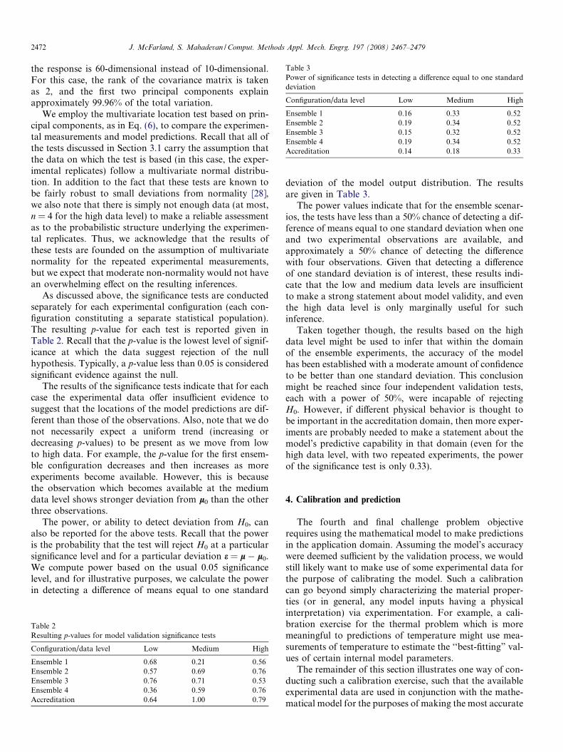
Table 3Power of significance tests in detecting a difference equal to one standarddeviation

Configuration/data level Low Medium High

Ensemble 1 0.16 0.33 0.52Ensemble 2 0.19 0.34 0.52Ensemble 3 0.15 0.32 0.52Ensemble 4 0.19 0.34 0.52Accreditation 0.14 0.18 0.33


the response is 60-dimensional instead of 10-dimensional.For this case, the rank of the covariance matrix is takenas 2, and the first two principal components explainapproximately 99.96% of the total variation.

We employ the multivariate location test based on prin-cipal components, as in Eq. (6), to compare the experimen-tal measurements and model predictions. Recall that all ofthe tests discussed in Section 3.1 carry the assumption thatthe data on which the test is based (in this case, the exper-imental replicates) follow a multivariate normal distribu-tion. In addition to the fact that these tests are known tobe fairly robust to small deviations from normality [28],we also note that there is simply not enough data (at most,n = 4 for the high data level) to make a reliable assessmentas to the probabilistic structure underlying the experimen-tal replicates. Thus, we acknowledge that the results ofthese tests are founded on the assumption of multivariatenormality for the repeated experimental measurements,but we expect that moderate non-normality would not havean overwhelming effect on the resulting inferences.

As discussed above, the significance tests are conductedseparately for each experimental configuration (each con-figuration constituting a separate statistical population).The resulting p-value for each test is reported given inTable 2. Recall that the p-value is the lowest level of signif-icance at which the data suggest rejection of the nullhypothesis. Typically, a p-value less than 0.05 is consideredsignificant evidence against the null.

The results of the significance tests indicate that for eachcase the experimental data offer insufficient evidence tosuggest that the locations of the model predictions are dif-ferent than those of the observations. Also, note that we donot necessarily expect a uniform trend (increasing ordecreasing p-values) to be present as we move from lowto high data. For example, the p-value for the first ensem-ble configuration decreases and then increases as moreexperiments become available. However, this is becausethe observation which becomes available at the mediumdata level shows stronger deviation from l0 than the otherthree observations.

The power, or ability to detect deviation from H0, canalso be reported for the above tests. Recall that the poweris the probability that the test will reject H0 at a particularsignificance level and for a particular deviation e = l � l0.We compute power based on the usual 0.05 significancelevel, and for illustrative purposes, we calculate the powerin detecting a difference of means equal to one standard

Table 2Resulting p-values for model validation significance tests

Configuration/data level Low Medium High

Ensemble 1 0.68 0.21 0.56Ensemble 2 0.57 0.69 0.76Ensemble 3 0.76 0.71 0.53Ensemble 4 0.36 0.59 0.76Accreditation 0.64 1.00 0.79

deviation of the model output distribution. The resultsare given in Table 3.

The power values indicate that for the ensemble scenar-ios, the tests have less than a 50% chance of detecting a dif-ference of means equal to one standard deviation when oneand two experimental observations are available, andapproximately a 50% chance of detecting the differencewith four observations. Given that detecting a differenceof one standard deviation is of interest, these results indi-cate that the low and medium data levels are insufficientto make a strong statement about model validity, and eventhe high data level is only marginally useful for suchinference.

Taken together though, the results based on the highdata level might be used to infer that within the domainof the ensemble experiments, the accuracy of the modelhas been established with a moderate amount of confidenceto be better than one standard deviation. This conclusionmight be reached since four independent validation tests,each with a power of 50%, were incapable of rejectingH0. However, if different physical behavior is thought tobe important in the accreditation domain, then more exper-iments are probably needed to make a statement about themodel’s predictive capability in that domain (even for thehigh data level, with two repeated experiments, the powerof the significance test is only 0.33).

4. Calibration and prediction

The fourth and final challenge problem objectiverequires using the mathematical model to make predictionsin the application domain. Assuming the model’s accuracywere deemed sufficient by the validation process, we wouldstill likely want to make use of some experimental data forthe purpose of calibrating the model. Such a calibrationcan go beyond simply characterizing the material proper-ties (or in general, any model inputs having a physicalinterpretation) via experimentation. For example, a cali-bration exercise for the thermal problem which is moremeaningful to predictions of temperature might use mea-surements of temperature to estimate the ‘‘best-fitting” val-ues of certain internal model parameters.

The remainder of this section illustrates one way of con-ducting such a calibration exercise, such that the availableexperimental data are used in conjunction with the mathe-matical model for the purposes of making the most accurate


predictions possible for the system response in the applica-tion domain. More specifically, we employ the Bayesian cal-ibration methodology outlined by Kennedy and O’Hagan[21], which purports to account for all uncertainties presentin the problem. That is, we obtain not only point estimatesas to the best-fitting parameters, but we obtain fully speci-fied uncertainty information regarding the parameterestimates, which is the result of both experimental uncer-tainty associated with the calibration data and ‘‘model inad-equacy”, which is associated with systematically biasedmodel predictions.

Section 4.1 gives a brief overview of the Kennedy andO’Hagan calibration framework, and Section 4.2 discussesthe issues associated with applying the methodology to thethermal challenge problem and presents the results of theanalysis. Section 4.3 discusses how the results of the cali-bration analysis can be used to predict the ‘‘probabilityof failure” in the application domain, thus assessing regu-latory compliance. In particular, Section 4.3 will focus onhow the uncertainty information obtained by the calibra-tion analysis can be used to make quantitative statementsregarding confidence in the ‘‘probability of failure”assessment.

4.1. Calibration under uncertainty: the Kennedy and

O’Hagan framework

A detailed discussion of Kennedy and O’Hagan’s Bayes-ian framework for the calibration of computer models isbeyond the scope of this paper, but the interested readeris referred to the authors’ original paper [21]. FollowingKennedy and O’Hagan (henceforth KOH), we considerclassifying the inputs to a computer simulation into twocategories. First, we define the calibration inputs, denotedby the vector h, as those inputs that ‘‘are supposed to takefixed but unknown values for all the observations that willbe used for calibration, and for all the instances of the trueprocess that we wish to use the calibrated model to pre-dict”. Thus, the calibration inputs are those inputs we wishto learn about through the calibration process. The secondcategory of inputs, defined by KOH as the variable inputsand denoted by the vector x, consists of all other inputs tothe model whose value might change as we use the model.These can also be thought of as ‘‘scenario-descriptor”

inputs, and generally describe the geometry, boundary con-ditions, and initial conditions associated with a particularsystem being modeled. The variable inputs are assumedto have known values for all of the experimental observa-tions used in the calibration process.

The full KOH formulation allows for ‘‘code uncer-tainty”, which describes the case in which the simulationis slow and/or expensive to execute, and only a finite num-ber of ‘‘runs” can be made. This can be done by treatingthe simulation as a Gaussian process that is ‘‘observed”

at those points for which runs are available. Since theheat-transfer model given in the thermal challenge problemis computationally simple, ‘‘code uncertainty” is not con-

sidered here. The treatment of code uncertainty during cal-ibration is described in detail in Kennedy and O’Hagan[21].

Following the notation used by KOH, the relationshipbetween the experimental observations zi, the computermodel output g(�,�), and the real process f(�) is given by

zi ¼ fðxiÞ þ ei ¼ gðxi; hÞ þ dðxiÞ þ ei; ð8Þ

where ei is the observation error associated with zi, and d(�)denotes the model inadequacy function. Note that variableinputs, x, depend on the experiment, whereas the calibra-tion parameters, h, are assumed to have a constant, but un-known, value.

The calibration process is based on Bayesian analysis(see, for example, [31]). Bayesian analysis represents degreeof belief using probability distributions, and allows priorbelief about uncertain parameters to be ‘‘updated” basedon observed data. With regards to calibration, the goal isto update our prior belief about the calibration parameters,h, based on the observed experimental responses, zi. Theresult is a complete ‘‘posterior” distribution for h whichrepresents the updated belief about the calibration param-eters. Thus, these results can be incorporated with esti-mates of the ‘‘model inadequacy”, or bias, to makepredictions, with ‘‘belief” intervals, about the response ofthe real system at an untested scenario, x*.

One feature which makes the KOH formulation so pow-erful is that the model inadequacy function, d(�), is treatedas a Gaussian process over the variable inputs x. In doingso, d is treated as a random quantity, and the relationbetween the model bias and the scenario-descriptors x ismodeled, which proves useful for making predictions ofthe process at untested locations.

A Gaussian process is defined by a mean function and acovariance function, which are functions of the variablesindexing the process, in this case x. For more informationon the use of Gaussian processes for modeling unknownfunctions, refer to [32,33].

We acknowledge several potential problem areas withregards to the modeling of the simulator bias term as a sta-tionary Gaussian process. In particular, when this modelinadequacy function is used to predict the value or uncer-tainty in the simulator bias outside the range of availabledata, then the statistics of the Gaussian process, i.e. itsmean and variance, come into play in a more pronouncedfashion. Such extrapolative inference will tend to rely heav-ily on the set of bases and coefficients chosen for the meanfunction, as well as the value of the process variance, whichis sometimes difficult to estimate. One particularly discon-certing feature is that if the usual equation for the condi-tional variance is used, the uncertainty in the bias will belimited to the process variance, regardless of how muchextrapolation is attempted. However, this pitfall can beavoided by using a more extensive formulation of the con-ditional variance (see, for example, [33,34]) which can growwithout bound. Even though some concerns do exist withregards to the model inadequacy formulation developed


by Kennedy and O’Hagan [21] for model calibration, wewould argue that modeling the bias function as a stationaryGaussian process still provides a more comprehensivetreatment of uncertainty than would be obtained if a sim-pler approach (e.g. no bias, or a deterministic constant)were taken. Given the formulation of Eq. (8), the proce-dure for doing calibration is to start with a prior probabil-ity distribution for h, denoted p(h), and use Bayes’ theoremto compute the posterior distribution given the observeddata, which is denoted f(h|z). Bayes’ theorem relates theprior and posterior distributions through a likelihood func-tion, as

f ðhjzÞ / pðhÞLðzjhÞ; ð9Þ

where L(z|h) is the likelihood function, which in terms ofcalibration relates the ‘‘likelihood” that the calibration in-puts h could have produced the observed response values z.

Although it is necessary to specify some joint prior dis-tribution for the calibration inputs, this does not mean thatit is necessary to have prior knowledge. It is possible to usevague, non-informative prior distributions to represent acomplete lack of knowledge with respect to the inputs,before observing the outputs. For inputs which have sup-port over the entire real line, this is most commonly doneusing independently uniform prior distributions, so thatthe joint prior distribution for all calibration inputs is

pðhÞ ¼ constant: ð10Þ

This prior distribution will result in a posterior which is ex-actly proportional to the likelihood function, so that all ofour knowledge comes from the data.

We may also incorporate bounds for any of the inputsinto this prior distribution, so that we have

pðhÞ ¼constant h 2 X

0; h 62 X

�ð11Þ

where the region X defines the bounds for the calibrationinputs h. This formulation will still yield a posterior thatis proportional to the likelihood, but it will also requirethat the posterior distribution lies inside X.

Given the model of Eq. (8), the form of the likelihoodfunction depends on the assumed probabilistic structurefor the experimental measurement errors, ei. Such errorsare typically assumed to follow a normal distribution (asis done by [21]), and this assumption will be made here(note that the model can theoretically accommodate anytype of error distribution). We will allow that the observa-tions can have different error variances, so that we haveei � N(0, ki).

Based on the above formulation (which is a slightsimplification of the full KOH formulation), the likelihoodfunction for z given h (which is sometimes written asL(h) because z is fixed) has the following probabilitydistribution:

zjh � NnðgþHb;Rexp þ RGPÞ; ð12Þ

where Nn(�,�) denotes a multivariate normal distribution, n

is the number of experimental observations in z, g = (g(x1,h), . . . ,g(xn, h))T, H is the matrix containing as rows the ba-sis functions corresponding to the mean function of d(�)evaluated at each xi, Rexp is a diagonal matrix with ele-ments ki, and RGP is the covariance matrix of the Gaussianprocess d(�) evaluated over all xi.

4.2. Calibration of the heat-transfer model

First, let us consider the classification of the heat-trans-fer model’s input parameters into the calibration inputsand the variable inputs. Clearly, there are two variableinputs, q and L, which describe the scenario and vary fromone experiment to the next; we thus have x = (q,L). Forthis model, the number of possible adjustable ‘‘calibrationparameters” is small, but several options still exist. The ini-tial temperature, Ti, although known to be 25 �C, mightstill be an effective calibration parameter, in the sense thatadjusting it slightly might lead to a better fit to experimen-tal data (as discussed in [21]). However, its role in adjustingmodel bias will be handled more fully by the model inade-quacy function, d(�), so we will hold Ti fixed at 25 �C.

Finally, the material properties, k and qC, although sub-ject to parametric variability, can also be useful as calibra-tion parameters. The method employed here is to treattheir means as fixed but unknown calibration parameters.In this case, we calibrate the mean values to give the bestfit to the data, while the variances remain at their originallyestimated values. In doing so, the role of the material prop-erties as stochastic inputs which impose variability on theoutput can still be maintained. The use of the calibrationresults for probability of failure estimation will be dis-cussed in more detail in Section 4.3. Thus, for the purposeof maintaining the variability imposed by the stochasticinputs, we take as the calibration inputs h = (lk,lqC).

We must also decide what particular system responsequantity of the heat-transfer model will be used for calibra-tion. Since we are ultimately interested in enhancing thepredictive capability of the model, we want to choose aquantity that is most relevant to the intended use of themodel for predictions in the application domain. Althoughit would be possible to calibrate using all measured temper-ature responses at each time instance, doing so would sig-nificantly increase the complexity of the analysis. Inaddition, the temperature responses show such strong lin-ear dependency that it is unlikely that much additionalinformation would be obtained. Finally, we note that theintended use of the model is to make predictions att = 1000 s only. For these reasons, we contend that the cal-ibration analysis should make use of temperature measure-ments corresponding to t = 1000 s only.

Next, there are several modeling choices which must bemade with regard to the Gaussian process d(�). First, amean function must be chosen. The role of the mean func-tion in Gaussian process modeling can be trivial in somecases, but it can also become important when the Gaussian

Fig. 1. Posterior mean of model inadequacy function, along with 80%confidence bounds (for L = 0.019).


process is used to predict the value of the process beyondthe range of observed data, particularly when systematictrends are present in the data. Based on observed trendsfor the heat-transfer model, and also to avoid over-param-eterization, we choose a linear mean function for d(�):

mðxÞ ¼ b0 þ b1qþ b2L; ð13Þ

where b = (b0,b1,b2)T are coefficients to be estimated.In order to fully specify the Gaussian process, we also

need a covariance function. The covariance function indi-cates how strongly related any two response values willbe, and is expressed in terms of x. Intuitively, we expectresponses which are similar in terms of x to be similar aswell in terms of their response values. In achieving this, sev-eral parametric covariance functions are possible [33]. Theform used here is the popular squared exponential, which isgiven by

Covðx; x0Þ ¼ r2 exp �Xd

i¼1

niðxi � x0iÞ2

" #; ð14Þ

where r2 is the process variance, d is the dimensionality ofx, and the ni are parameters related to the inverse correla-tion length of the process with respect to each input. A rel-atively large value ni indicates that the input xi is relativelyimportant in predicting the value of the process response.

We will treat the parameters governing the Gaussianprocess for d(�) as fixed constants, and before proceedingwith the calibration, their values must be estimated basedon the data. Maximum Likelihood Estimation (MLE) isused here to estimate the values for b, n, and r2. Refer to[35,36] for the implementation details associated withMLE for Gaussian processes. The method of MaximumLikelihood Estimation computes parameter estimatesbased on observed values of the process and the corre-sponding inputs, x, associated with each. Note that theprocess being modeled is the simulator bias, given byzi � g(xi, h), which in fact depends on h. However, toobtain a plausible estimate to the simulator bias, we esti-mate the model inadequacy function using a fixed, nominalvalue for h. In this case, we use the mean values of thematerial properties, based on the material characterizationdata.

Once the parameters of the Gaussian process are esti-mated, Hb and RGP in Eq. (12) can be computed usingEqs. (13) and (14). To evaluate the likelihood function,we also need estimates for ki, the experimental error vari-ance associated with each observation. Since for this prob-lem we have available repeated experimental observationsat each particular configuration, we will use a separatevalue of k for each configuration, where each is estimatedas the sample variance of the corresponding experimentalobservations.

Finally, we must choose a prior probability distributionfor h. For the challenge problem, we choose the vague priordistribution given by Eq. (10), so that the calibrationresults will be dominated by the data.

Computation of the posterior distribution is based onthe evaluation of Eq. (9), which due to the complexity ofthe multidimensional integral required to make the left-hand side integrate to one generally requires specializedtechniques. Markov Chain Monte Carlo (MCMC) sam-pling [37,38] is a simulation scheme which is commonlyused in Bayesian analysis; specifically, the componentwiseversion of the Metropolis algorithm [39] is used here. How-ever, keep in mind that we are not necessarily interested inthe posterior distribution of h as such, but we are in factconcerned with the posterior distribution of the real pro-cess at the application domain. Fortunately, the MCMCsampling procedure allows us to easily obtain such quanti-ties as by-products of the updating process.

To predict the value of the real process at an untestedscenario given by inputs x*, we might choose as our estima-tor the posterior mean of the real process, given by

E½fðx�Þjz� ¼Z

HE½fðx�Þjh; z�f ðhjzÞdh; ð15Þ

where the posterior mean conditional on h is given by

E½fðx�Þjh; z� ¼ gðx�; hÞ þ E½dðx�Þjz�; ð16Þ

and E[d(x*)|z] is the posterior mean of the model inade-quacy function at x*.

For the thermal problem, the posterior mean of themodel inadequacy function is plotted in Fig. 1 versus q,along with 80% confidence bounds based on Var[d(x)|z];L is held constant at 0.019 m, which corresponds to thevalue at the application configuration.

Section 4.3 discusses how these results can be used toestimate the probability of failure of a device in the appli-cation domain, along with confidence bounds for theassessment.


4.3. Assessment of regulatory compliance

The fourth and final objective for the thermal challengeproblem asks the analyst to provide both an assessment asto whether or not the device will meet regulatory require-ments and a statement of confidence in this assessment.The probability of failure for the device in the applicationconfiguration is defined as

pf ¼ P ðT ðt ¼ 1000 sÞ > 900 �CÞ; ð17Þ

and regulatory compliance is said to be achieved if theprobability of failure is less than 0.01.

One of the difficulties in using the above Bayesian cali-bration results for probability of failure prediction is thatwe must make sure to differentiate between aleatory (truevariability) and epistemic (lack of knowledge) uncertain-ties. The probability of failure condition defined by Eq.(17) is the result of specimen-to specimen variability man-ifested through the treatment of the material properties k

and qC as random variables (aleatory uncertainty). How-ever, in the Bayesian calibration analysis, we have treatedh = (lk,lqC) as a random variable, but this is an epistemicuncertainty, and must be considered separately because itdoes not contribute to actual variability of the response.

First, we note that for any particular realization of h andd, there is an associated value of pf which can be computedbased on rk and rqC. We define this conditional failureprobability as

pf jh; d ¼Z

E½fðx�Þjh;z�>900 �Cf ðk; qCÞdk dqC; ð18Þ

where f(k,qC) is the joint probability density function for kand qC, which are treated as independent random variableswith probability distributions k � N(lk,rk) and qC � N

(lqC,rqC). This conditional failure probability can be com-puted with simple Monte Carlo simulation.

Based on the results of the calibration analysis, we maytake as our best estimate of pf the value obtained by aver-aging over the posterior distribution of h, such that theexpected value of pf is given by

E½pf � ¼Z

Hðpf jh;E½djz�Þf ðhjzÞdh: ð19Þ

Given that f(h|z) is constructed using MCMC simula-tion, the draws of h from its posterior can be used as ran-dom samples for the outer Monte Carlo simulation loopneeded to compute the expectation of pf over h. Applyingthis method, we obtain E[pf] = 0.166.

In order to judge the uncertainty associated with theabove estimate of pf, we propose an approximate methodfor estimating reasonable upper and lower bounds for thefailure probability. Our heuristic approach attempts toaccount for:

1. Residual uncertainty in h after calibration (given by itsposterior distribution).

2. Residual uncertainty in d after calibration (again givenby its posterior distribution).

3. Uncertainty present in the estimates of rk and rqC dueto having estimated them based on finite data.

Residual uncertainty in h and d can be accounted for ina straightforward manner by constructing the posterior dis-tribution for pf implied by the posterior distributions of h

and d. Inferences about the uncertainty in pf due to thesesources can then be made based on its posteriordistribution.

It is not as straightforward, on the other hand, toaccount for uncertainty in the estimates of rk and rqC, asthis uncertainty did not play a role in the Bayesian calibra-tion analysis. We propose the following heuristic approachbased on confidence intervals for rk and rqC:

1. Construct standard confidence intervals for rk and rqC

to get upper and lower bounds.2. For each set of bounds, conduct the failure probability

analysis to get a corresponding distribution for pf:a. Fix rk and rqC at their lower bounds, and con-

struct the posterior distribution of pf based onthe posterior distribution of h and d. Based onuncertainty in rk and rqC, this distribution repre-sents a lower bound for pf, so we denote its CDFby Fl(pf).

b. Now we fix rk and rqC at their upper bounds toconstruct Fu(pf) in the same manner.

3. To obtain overall reasonable bounds for pf, we take the0.05 level from Fl(pf) and the 0.95 level from Fu(pf). Con-sider the lower bound for pf: uncertainty in rk and rqC isaccounted for in the construction of Fl(pf); to accountfor the uncertainty in h and d, we take the 5th percentilefrom this distribution. Similarly, to get an overall upperbound, we take the 95th percentile from Fu(pf).

For step 1, we apply the usual method to construct con-fidence intervals for rk and rqC (see, for example, [40]),which carries the assumptions that either the underlyingvariables k and qC follow normal distributions or the cen-tral limit theorem applies. The confidence intervals are con-structed based on all 30 material characterization datapoints (the estimation for rk is based on the residuals ofa linear regression on T, as discussed in Section 2, so thatthe number of degrees of freedom becomes 28 instead of29). We consider the 95% confidence intervals for thepopulation parameters, which yields hrki0.95 = [0.00373,0.00636] and hrqCi0.95 = [2.89E4,4.87E4].

We then consider both the lower and upper bound pairsto obtain the two distributions Fl(pf) and Fu(pf), discussedin step 2. Finally, to obtain the overall bounds for pf, wetake the 0.05 level from Fl(pf) and the 0.95 level from Fu(pf),which gives [0.036, 0.336]. We emphasize that these boundsfor pf can not be interpreted in the usual way for statisticalconfidence intervals, as such confidence intervals have a


particular and rigorously defined meaning. The boundsreported here represent our best estimate for the magnitudeof the uncertainty associated with our nominal estimate ofpf (which is 0.166). We have attempted to account for bothuncertainty in the characterization of the material propertyvariability, as well as residual uncertainty after calibrationin the calibration parameters.

Based on the above bounds for pf, our conclusion is thatwe do not believe that the device will meet the regulatoryrequirement defined by Eq. (17), which specifies that theprobability of failure must be less than 0.01. However,the bounds also indicate that there is a large amount ofuncertainty associated with the assessment of the failureprobability, suggesting that the collection of more datamay be warranted before making a high-consequencedecision.

Finally, we acknowledge that the construction of theabove bounds is by no means purely objective. We hadto choose values for the significance level associated withthe confidence intervals for rk and rqC, as well as the signif-icance level at which we ‘‘pick off” values from Fl(pf) andFu(pf). In both cases, we choose the standard 95% levelto obtain what we feel are reasonable bounds, but differentchoices of the significance level will of course produce dif-ferent bounds.

5. Conclusions

First, this paper illustrates how multivariate significancetesting can be used to carry out quantitative validationassessment of a computer simulation having multivariateoutput. Moreover, the use of principal components analy-sis is demonstrated for dealing with very highly correlatedoutputs which would otherwise cause problems with singu-lar covariance. Although the given model is fast to evalu-ate, the use of the above validation methodology for real-world simulations which are slow and/or expensive mayrequire the use of a response surface approximation, suchas the one developed by Isukapalli et al. [24].

Having obtained the distribution of the model output,the hypothetical experimental data are then comparedagainst it using Hotelling’s T2 statistic, which is a multivar-iate extension of Student’s t statistic. This comparison iscarried out at multiple different ‘‘configurations” (combi-nations of geometry and boundary conditions) and usingthree different amounts of validation data. It is found thatin none of the cases do we have significant evidence againstthe null hypothesis that the locations of the distributions ofthe model output and experimental data are the same.

Although the results suggest model validity, we alsokeep in mind that lack of achieved significance againstthe null hypothesis may not be due simply to the truth ofthe null, but possibly also to having small sample sizes(small amounts of experimental data). This issue can beexplored quantitatively be considering the power of thetests, which is an indication of the ability of the tests to dis-cern between the competing hypotheses. The power is com-

puted by first specifying the deviation from the null whichis of interest (in this case, how far apart the predictions canbe from the observations before the difference is impor-tant). To illustrate the computations, we consider thepower of the tests in detecting a difference in means equalto one standard deviation of the response values. Theresults indicate that even for the cases when data from fourrepeated experiments are available (the high data level inthe ensemble validation domain), the significance tests onlyhave about a 50% probability of discerning the difference.Thus, an appropriate conclusion might be to say thatalthough we do not have enough evidence to suggest thatthe model predictions are statistically inconsistent withthe experiments, more data from repeated experimentsare needed before a strong conclusion about model validitycan be reached.

In addition, we note that establishing the validity of themathematical model within the validation database doesnot imply that its accuracy will be sufficient for use in theapplication domain, which corresponds to different geome-try and boundary conditions than those used in the exper-iments. Based purely on the validation data, it is notpossible to divine what additional physical phenomenamay become important for conditions beyond those testedin the lab. For example, nonlinearities in the thermal sys-tem may become pronounced for higher values of appliedheat flux, rendering the mathematical model’s accuracyunacceptable for predicting the system’s behavior in theapplication domain. One recommendation for dealing withthese issues would be to make use of all sources of informa-tion when inferring the model’s validity at the applicationdomain. If possible, the quantitative validation resultsshould be combined with expert opinion regarding poten-tial changes in the physical system’s behavior. Combiningthese sources of information may be difficult and tend tobe more qualitative in nature, but it would be in hopes ofpreventing over-confidence in the model’s accuracy in theapplication domain, for which no data are available.Addressing how multiple pieces of validation data can beused collectively to infer model validity for an untestedconfiguration is certainly an interesting avenue for futurework.

The second part of this paper (Section 4) illustrates amethod for using the given model to assess regulatory com-pliance by first calibrating the model using the Bayesianframework developed by Kennedy and O’Hagan [21].The calibration exercise achieves several goals. First, thesystematic bias of the model predictions is characterized,and the methodology attempts to account for how this biasextrapolates to the application domain. In addition, themethod accounts for the uncertainty present in the experi-mental data used for calibration, resulting in an estimate ofthe remaining uncertainty when the model is then used forprediction. Finally, in estimating the confidence in ourassessment of pf, we also attempt to account for the uncer-tainty associated with the estimates of the distributionparameters of the material properties. In particular, the


variances of these properties play a crucial role in theresulting estimates of pf, since they are what drive the var-iability of the model output. Because we have only a finitedata set with which to estimate their variances, we believethat comprehensive analysis of the probability of failureshould account for the uncertainty associated with any esti-mates of the material property variability.

Although the work discussed herein does make use ofpreviously published research, it addresses important ques-tions pertaining to the application of some of these existingmethods. For example, while the significance testingapproach has been used previously for model validationassessment, we feel there are still related questions whichneed further exploration. Many different model validationapplications may require various and differing formula-tions of the hypothesis testing problem. With regards tomodel calibration under uncertainty, we do make use ofthe calibration methodology developed by Kennedy andO’Hagan [21], but we provide additional, new ideas foraccounting for uncertainty due to the fact that some prob-ability distribution parameters are estimated based on finitedata sets.

Acknowledgements

The research reported in this paper was partly supportedby funds from the National Science Foundation, throughthe IGERT multidisciplinary doctoral program in Riskand Reliability Engineering at Vanderbilt University, andpartly by funds from Sandia National Laboratories, Albu-querque, NM (contract no. BG-7732; project monitors: Dr.Thomas Paez, Dr. Laura P. Swiler, and Dr. Martin Pilch).The support is gratefully acknowledged.

References

[1] K.J. Dowding, M. Pilch, R.G. Hills, Formulation of the thermalproblem, Comput. Methods Appl. Mech. Engrg. (2007).

[2] W. Oberkampf, M. Barone, Measures of agreement between compu-tation and experiment: validation metrics, J. Comput. Phys. 217(2006) 5–36.

[3] W. Oberkampf, T. Trucano, Verification and validation in compu-tational fluid dynamics, Sandia National Laboratories, SAND2002-0529, 2002.

[4] R. Sargent, Validation and verification of simulation models, in:Proceedings of the 2004 Winter Simulation Conference, Washington,DC, 2004.

[5] O. Balci, Verification, validation, and accreditation of simulationmodels, in: Proceedings of the 29th Conference on Winter Simulation,Atlanta, GA, 1997.

[6] R.G. Hills, T.G. Trucano, Statistical validation of engineering andscientific models: a maximum likelihood based metric, SandiaNational Laboratories, SAND2001-1783, 2002.

[7] T. Paez, A. Urbina, Validation of mathematical models of complexstructural dynamic systems, in: Proceedings of the Ninth Interna-tional Congress on Sound and Vibration, Orlando, FL, 2002.

[8] R.G. Hills, I. Leslie, Statistical validation of engineering and scientificmodels: validation experiments to application, Sandia NationalLaboratories, SAND2003-0706, 2003.

[9] K. Dowding, R.G. Hills, I. Leslie, M. Pilch, B.M. Rutherford, M.L.Hobbs, Case study for model validation: assessing a model for

thermal decomposition of polyurethane foam, Sandia NationalLaboratories, SAND2004-3632, 2004.

[10] B.M. Rutherford, K. Dowding, An approach to model validation andmodel-based prediction – polyurethane foam case study, SandiaNational Laboratories, SAND2003-2336, 2003.

[11] W. Chen, L. Baghdasaryan, T. Buranathiti, J. Cao, Model validationvia uncertainty propagation, AIAA J. 42 (2004) 1406–1415.

[12] S. Mahadevan, R. Rebba, Validation of reliability computationalmodels using Bayes networks, Reliab. Engrg. Syst. Safety 87 (2005)223–232.

[13] R. Rebba, S. Mahadevan, S. Huang, Validation and error estimationof computational models, Reliab. Engrg. Syst. Safety 91 (2006) 1390–1397.

[14] X. Jiang, S. Mahadevan, Bayesian risk-based decision method formodel validation under uncertainty, Reliab. Engrg. Syst. Safety 92(2007) 707–718.

[15] K. Campbell, A brief survey of statistical model calibration ideas, in:International Conference on Sensitivity Analysis of Model Output,Santa Fe, NM, 2004.

[16] T. Trucano, L. Swiler, T. Igusa, W. Oberkampf, M. Pilch, Calibra-tion, validation, and sensitivity analysis: what’s what, Reliab. Engrg.Syst. Safety 91 (2006) 1331–1357.

[17] A. Vecchia, R. Cooley, Simultaneous confidence and predictionintervals for nonlinear regression models, with application to agroundwater flow model, Water Resources Res. 23 (1987) 1237–1250.

[18] K. Beven, A. Binley, The future of distributed models: modelcalibration and uncertainty prediction, Hydrol. Process. 6 (1992) 279–298.

[19] J. Stigter, M. Beck, A new approach to the identification of modelstructure, Environmetrics 5 (1994) 315–333.

[20] H. Banks, Remarks on uncertainty assessment and management inmodeling and computation, Math. Comput. Modell. 33 (2001) 39–47.

[21] M.C. Kennedy, A. O’Hagan, Bayesian calibration of computermodels, J. Roy. Stat. Soc. Ser. B 63 (2001) 425–464.

[22] H. Lilliefors, On the Kolmogorov–Smirnov test for normality withmean and variance unknown, J. Am. Stat. Assoc. 62 (1967) 399–402.

[23] S. Shapiro, M. Wilk, An analysis of variance test for normality(complete samples), Biometrika 52 (1965) 591–611.

[24] S.S. Isukapalli, A. Roy, P.G. Georgopoulos, Stochastic ResponseSurface Methods (SRSMs) for uncertainty propagation: applicationto environmental and biological systems, Risk Anal. 18 (1998) 351–363.

[25] O. Balci, R. Sargent, A methodology for cost-risk analysis in thestatistical validation of simulation models, Commun. ACM 24 (4)(1981) 190–197.

[26] O. Balci, R. Sargent, Validation of simulation models via simulta-neous confidence intervals, Am. J. Math. Manage. Sci. 4 (3/4) (1984)375–406.

[27] O. Balci, R. Sargent, Validation of multivariate response simulationmodels by using Hotelling’s two-sample T2 test, Simulation 39 (1982)185–192.

[28] M. Srivastava, Methods of Multivariate Statistics, John Wiley andSons, Inc., New York, 2002.

[29] R. Rebba, S. Mahadevan, Validation of models with multivariateoutput, Reliab. Engrg. Syst. Safety 91 (2006) 861–871.

[30] B. Efron, R. Tibshirani, An Introduction to the Bootstrap, Chapmanand Hall, New York, 1993.

[31] P. Lee, Bayesian Statistics, an Introduction, Oxford University Press,Inc., New York, 2004.

[32] C. Rasmussen, Evaluation of Gaussian processes and other methodsfor non-linear regression, Doctoral Thesis, University of Toronto,1996.

[33] B. Ripley, Spatial Statistics, John Wiley, New York, 1981.[34] T.J. Santner, B. Williams, W. Notz, The Design and Analysis of

Computer Experiments, Springer-Verlag, New York, 2003.[35] K. Mardia, R. Marshall, Maximum likelihood estimation of models

for residual covariance in spatial regression, Biometrika 71 (1984)135–146.


[36] J. Martin, T. Simpson, Use of Kriging models to approximatedeterministic computer models, AIAA J. 43 (2005) 853–863.

[37] N. Metropolis, A. Rosenbluth, M. Rosenbluth, A. Teller, E. Teller,Equations of state calculations by fast computing machines, J. Chem.Phys. 21 (1953) 1087–1092.

[38] S. Chib, E. Greenberg, Understanding the Metropolis–Hastingsalgorithm, Am. Stat. 49 (1995) 327–335.

[39] W.K. Hastings, Monte Carlo sampling methods using Markov chainsand their applications, Biometrika 57 (1970) 97–109.

[40] A. Haldar, S. Mahadevan, Probability, Reliability, and StatisticalMethods in Engineering Design, John Wiley and Sons, Inc., NewYork, 2000.

Multivariate significance testing and model calibration under uncertainty

Documents

Transcript of Multivariate significance testing and model calibration under uncertainty