Presentation Topic

Multivariate Regression Analysis

Learning Objectives

– Introduction To Multivariate Regression Analysis.

– Multivariate Least Squares Estimation.– Test of Overall Regression

Multivariate Analysis

Multivariate analysis (MVA) is based on the statistical principle of multivariate statistics, which involves observation and analysis of more than one variable at the same time.

Regression

A statistical process for estimating the relationship among dependent and independent variables.

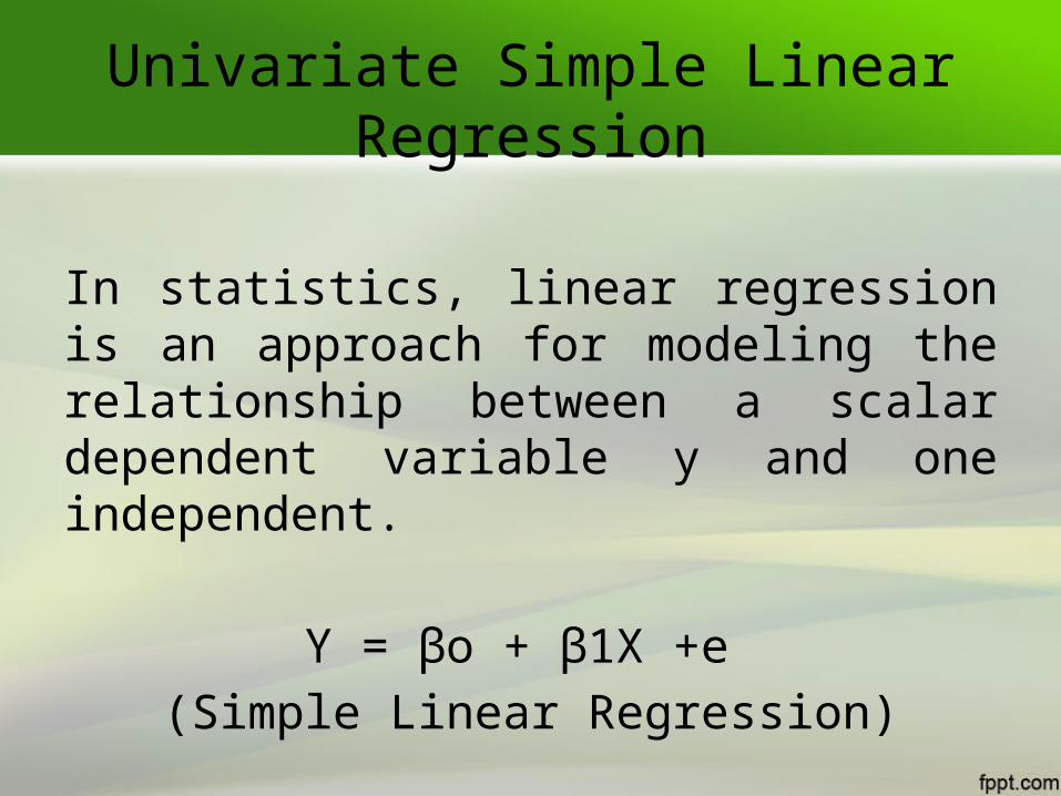
Univariate Simple Linear Regression

In statistics, linear regression is an approach for modeling the relationship between a scalar dependent variable y and one independent.

Y = βo + β1X +e (Simple Linear Regression)

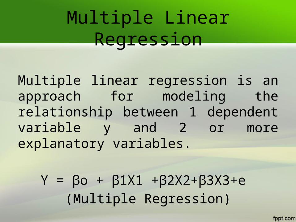
Multiple Linear Regression

Multiple linear regression is an approach for modeling the relationship between 1 dependent variable y and 2 or more explanatory variables.

Y = βo + β1X1 +β2X2+β3X3+e (Multiple Regression)

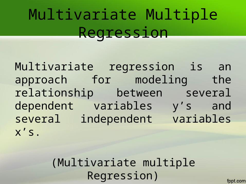
Multivariate Multiple Regression

Multivariate regression is an approach for modeling the relationship between several dependent variables y’s and several independent variables x’s.

(Multivariate multiple Regression)

Multivariate Multiple Regression

Where , ,

and

Types Of Independent Variables

There are two basic types of independent variables.1. MULTIPLE REGRESSION: FIXED x’s2. MULTIPLE REGRESSION: RANDOM x’s

1-MULTIPLE REGRESSION: FIXED x’s

In some experimental situations, the x ’s are fixed, that is, under the control of the experimenter. For example, a researcher may wish to relate yield per acre and nutritional value to level of application of various chemical fertilizers. The experimenter can choose the amount of chemicals to be applied and then observe the changes in the yield and nutritional responses.

2-MULTIPLE REGRESSION: RANDOM x’s

In some cases all x ’s are random variables and are therefore not under the control of the researcher. A person is chosen at random, and all the y ’s and x ’s are measured, or observed, for that person.

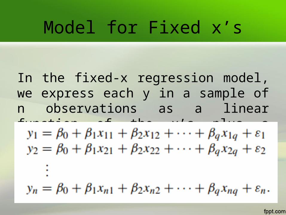
Model for Fixed x’s

In the fixed-x regression model, we express each y in a sample of n observations as a linear function of the x’s plus a random error, ε

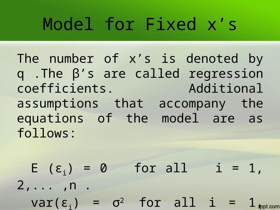
The number of x’s is denoted by q .The β’s are called regression coefficients. Additional assumptions that accompany the equations of the model are as follows:

E (εi) = 0 for all i = 1, 2,... ,n .

var(εi) = σ2 for all i = 1, 2,... ,n .

cov(εi,εj) = 0 for all i ≠ j .

Model for Fixed x’s

Matrix Notation

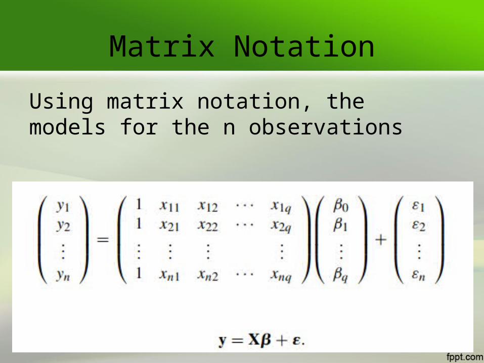
Using matrix notation, the models for the n observations

Least Squares Estimation in the Fixed- x Model

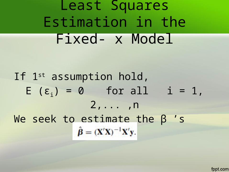
If 1st assumption hold, E (εi) = 0 for all i = 1, 2,... ,n

We seek to estimate the β ’s

Least Squares Estimation in the Fixed- x Model

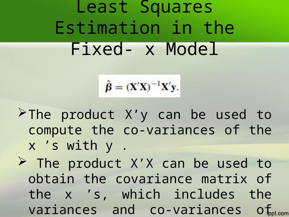
The product X’y can be used to compute the co-variances of the x ’s with y .

The product X’X can be used to obtain the covariance matrix of the x ’s, which includes the variances and co-variances of the x ’s.

Test of Overall Regression

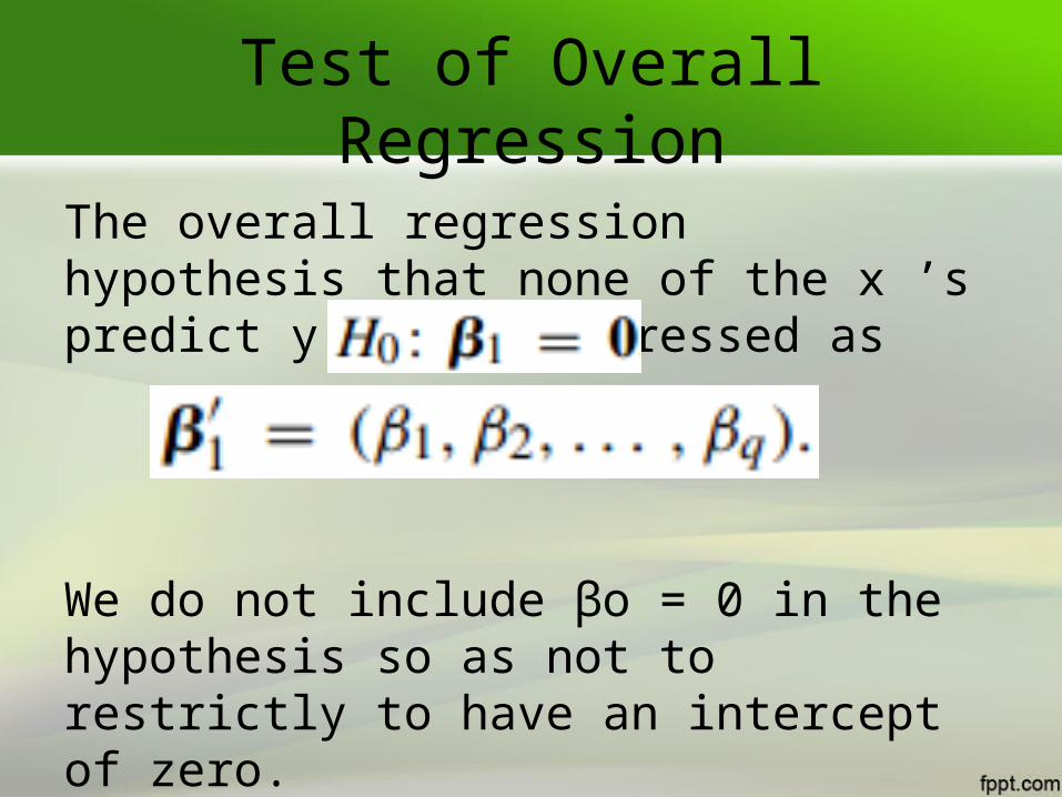
The overall regression hypothesis that none of the x ’s predict y can be expressed as

We do not include βo = 0 in the hypothesis so as not to restrictly to have an intercept of zero.

Test of Overall Regression

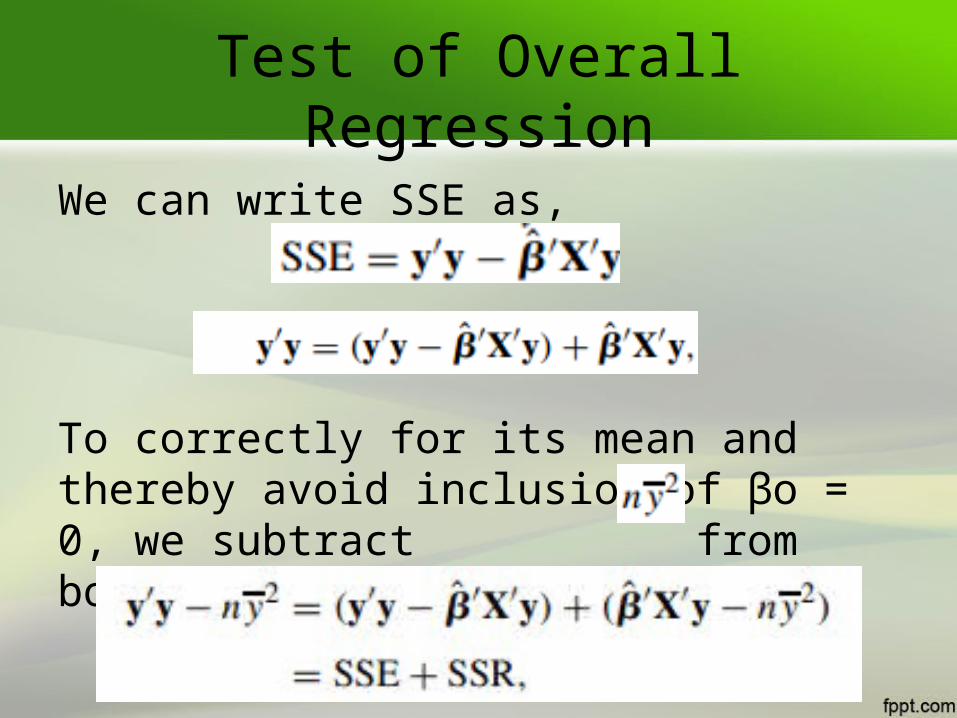
We can write SSE as,

To correctly for its mean and thereby avoid inclusion of βo = 0, we subtract from both sides of to obtain

Test of Overall Regression

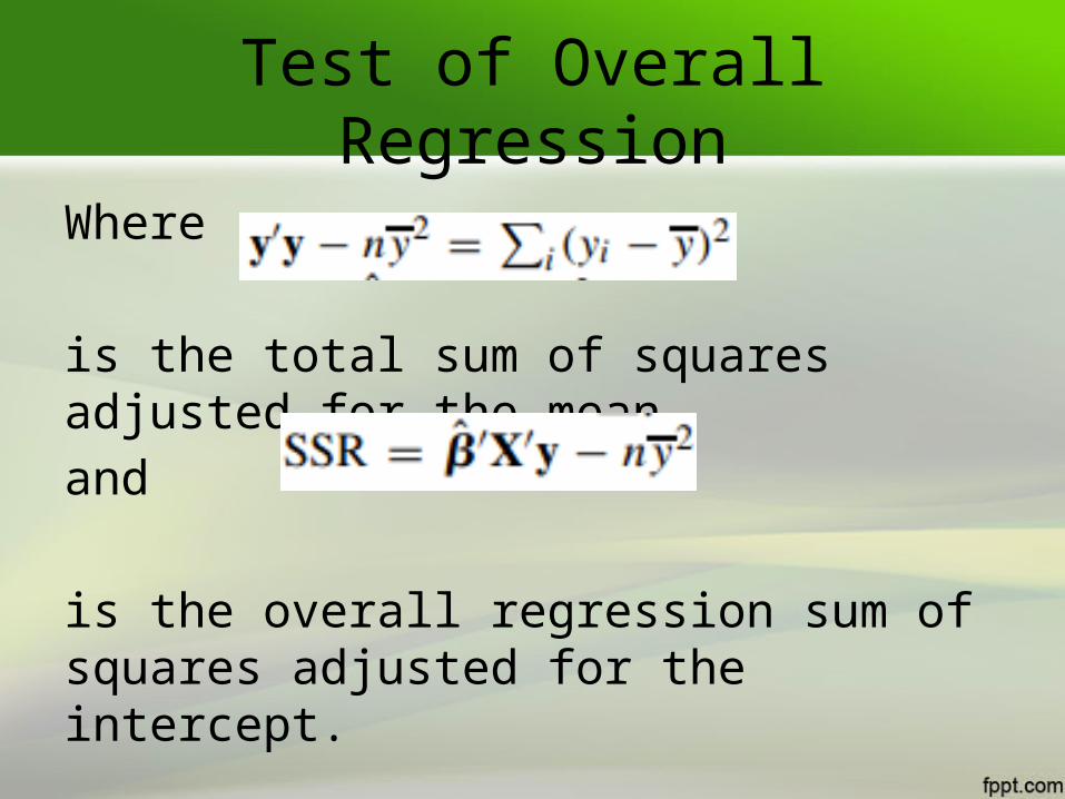
Where

is the total sum of squares adjusted for the meanand

is the overall regression sum of squares adjusted for the intercept.

Test of Overall Regression

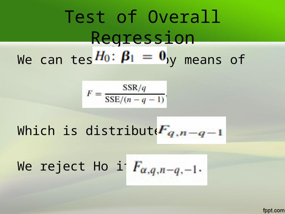
We can test by means of

Which is distributed as

We reject Ho if F >