Multivariate empirical mode decomposition

Multivariate empirical mode decompositionAuthor(s): N. Rehman and D. P. MandicSource: Proceedings: Mathematical, Physical and Engineering Sciences, Vol. 466, No. 2117 (8May 2010), pp. 1291-1302Published by: The Royal SocietyStable URL: http://www.jstor.org/stable/25661497 .

Accessed: 12/06/2014 19:56

Your use of the JSTOR archive indicates your acceptance of the Terms & Conditions of Use, available at .http://www.jstor.org/page/info/about/policies/terms.jsp

.JSTOR is a not-for-profit service that helps scholars, researchers, and students discover, use, and build upon a wide range ofcontent in a trusted digital archive. We use information technology and tools to increase productivity and facilitate new formsof scholarship. For more information about JSTOR, please contact [email protected].

.

The Royal Society is collaborating with JSTOR to digitize, preserve and extend access to Proceedings:Mathematical, Physical and Engineering Sciences.

http://www.jstor.org

This content downloaded from 194.29.185.109 on Thu, 12 Jun 2014 19:56:43 PMAll use subject to JSTOR Terms and Conditions

http://www.jstor.org/action/showPublisher?publisherCode=rsl

http://www.jstor.org/stable/25661497?origin=JSTOR-pdf

http://www.jstor.org/page/info/about/policies/terms.jsp


PROCEEDINGS -OF- A Proc. R. Soc. A (2010) 466, 1291-1302

THE ROYAL ?ik doi:10.1098/rspa.2009.0502 SOCIETY Alk Published online 23 December 2009

Multivariate empirical mode decomposition By N. Rehman* and D. P. Mandic

Department of Electrical and Electronic Engineering, Imperial College London, London SW7 2AZ, UK

Despite empirical mode decomposition (EMD) becoming a de facto standard for

time-frequency analysis of nonlinear and non-stationary signals, its multivariate extensions are only emerging; yet, they are a prerequisite for direct multichannel data

analysis. An important step in this direction is the computation of the local mean, as the concept of local extrema is not well defined for multivariate signals. To this end, we propose to use real-valued projections along multiple directions on hyperspheres (n-spheres) in order to calculate the envelopes and the local mean of multivariate signals, leading to multivariate extension of EMD. To generate a suitable set of direction vectors, unit hyperspheres (n-spheres) are sampled based on both uniform angular sampling methods and quasi-Monte Carlo-based low-discrepancy sequences. The potential of the proposed algorithm to find common oscillatory modes within multivariate data is demonstrated by simulations performed on both hexavariate synthetic and real-world human motion signals.

Keywords: multivariate signal analysis; empirical mode decomposition; intrinsic mode

functions; multiscale analysis; inertial body sensors; human motion analysis

1. Introduction

The empirical mode decomposition (EMD) algorithm is a fully data-driven method designed for multiscale decomposition and time-frequency analysis of real-world signals (Huang et al 1998), whereby the original signal is modelled as a linear combination of intrinsic oscillatory modes, called intrinsic mode functions

(IMFs). The IMFs are defined so as to exhibit locality in time and to represent a single oscillatory mode; the subsequent application of Hilbert transform

provides meaningful instantaneous frequency estimates (the so-called Hilbert

Huang transform) (Huang & Shen 2005). Owing to no a priori assumptions regarding the data nature, EMD has found applications in the analysis of nonlinear and non-stationary signals (e.g. Duffy 2004; Gautama et al 2004; Janosi & Muller 2005; Wu & Hu 2006; Huang & Wu 2008; Lin et al 2009).

The recent advances in physics and engineering have brought to light new

problems dealing with complexity, uncertainty, nonlinearity and multichannel

dynamics (Gautama et al 2004; Mandic & Goh 2009); these signals are, however,

* Author for correspondence ([email protected]).

Received 25 September 2009

Accepted 20 November 2009 1291 This journal is ? 2009 The Royal Society



1292 TV. Rehman and D. P. Mandic

almost invariably processed channel-wise (e.g. Duffy 2004; Janosi & Muller 2005; Wu & Hu 2006; Huang & Wu 2008). Extensions of standard EMD to multivariate signals are, therefore, a prerequisite for the accurate data-driven time-frequency analysis of such processes. In addition, joint analysis of multiple oscillatory components within a higher dimensional signal also helps to circumvent the mode

alignment problem1 (Looney & Mandic 2009) experienced with standard EMD; in the complex domain, this has proven to facilitate, e.g., the synchronization of

multichannel EEG signals and image fusion (Mandic et al. 2008; Looney & Mandic

2009). Recent multivariate extensions of EMD include those suitable for the

processing of bivariate (e.g. Tanaka Sz Mandic 2006; Altaf et al 2007; Rilling et al 2007) and trivariate (Rehman & Mandic in press) signals; however, general original n-variate extensions of EMD are still lacking, and are subject of this work.

The key issue in EMD algorithm is the computation of the local mean of the original signal, a step which depends critically on finding the local extrema.

However, for multivariate signals, this is not straightforward; for instance, the

complex and quaternion fields are not ordered (Mandic & Goh 2009). We

propose to alleviate this problem by using multiple real-valued projections of the

signal; the extrema of such projected signals are then interpolated component wise to yield the desired multidimensional envelopes of the signal. In our

proposed multivariate extension of EMD, we choose a suitable set of direction vectors in n-dimensional spaces by using: (i) uniform angular coordinates and

(ii) low-discrepancy pointsets stemming from quasi-Monte Carlo methods. It is shown that a set of direction vectors based on uniform sampling in the

angular coordinate system is convenient to deal with; however, it yields non

uniformly distributed direction vectors. The approach based on low-discrepancy pointsets (Niederreiter 1992) provides a more uniform distribution of direction vectors (Cui & Freeden 1997), and hence more accurate local mean estimates in n-dimensional spaces.

This paper is organized as follows: bivariate and trivariate extensions of EMD are first discussed in ?2. Section 3 introduces the proposed multivariate EMD method and analyses choices for a set of direction vectors in n-dimensional

spaces. Section 4 illustrates the mode alignment property of the proposed method on a synthetic hexavariate signal and on multivariate processing of real-world orientation data.

2. Existing multivariate extensions of EMD

EMD is a fully data-driven method for the multiscale analysis of nonlinear and

non-stationary real-world signals (Huang et al 1998). It decomposes the original

signal into a finite set of amplitude- and/or frequency-modulated (AM/FM) components, termed IMFs, which represent its inherent oscillatory modes. More

specifically, for a real-valued signal x(k), the standard EMD finds a set of TV

^ode alignment in multivariate data corresponds to finding a set of common scales/modes across

different components (variates) of a multivariate signal, thus ensuring that the IMFs are matched

both in the number and in scale properties.

Proc. R. Soc. A (2010)



Multivariate EMD 1293

IMFs {ci(k)}f=1, and a monotonic residue signal r(fc), so that N

x(k) = J2^(k) + r(k). (2.1) i=\

To ensure well-behaved intrinsic oscillations, IMFs Ci(k) are defined so as to have

symmetric upper and lower envelopes, with the number of zero crossings and the number of extrema differing at most by one. An iterative process called the

sifting algorithm is employed to extract IMFs; for illustration, a sifting procedure for obtaining the first IMF from the signal x'(k) is outlined in algorithm 1.

Algorithm 1. The standard EMD algorithm.

1. Find the locations of all the extrema of x'(k). 2. Interpolate (using cubic spline interpolation) between all the minima

(respectively maxima) to obtain the lower signal envelope, em[n(k) (respectively ^max(^))

3. Compute the local mean m(k) = [emin(A;) + emax(fc)]/2. 4. Subtract the mean from the signal to obtain the 'oscillatory mode'

s(k) = x\k) -

m(k). 5. If s(k) obeys the stopping criteria, then we define d{k) = s(k) as an IMF,

otherwise set x'(k) =

s(k) and repeat the process from step 1.

Once the first IMF is obtained, the same procedure is applied iteratively to the residual r(k) = x(k)

? d(k) to extract the remaining IMFs. The standard stopping

criterion terminates the sifting process only after the above condition for an IMF is met for S consecutive times (Huang et al. 2003).

(a) Bivariate/complex extensions of EMD

The first complex extension of EMD was proposed by Tanaka Sz Mandic (2006); it employed the concept of analytical signal and subsequently applied standard

EMD to analyse complex/bivariate data; however, this method cannot guarantee an equal number of real and imaginary IMFs, thus limiting its applications. An extension of EMD which operates fully in the complex domain was first proposed by Altaf et al (2007), termed rotation-invariant EMD (RI-EMD). The extrema of a complex/bivariate signal are chosen to be the points where the angle of the derivative of the complex signal becomes zero, that is, based on the change in the phase of the signal. The signal envelopes are produced by using component wise spline interpolation, and the local maxima and minima are then averaged to obtain the local mean of the bivariate signal.

The RI-EMD algorithm uses effectively only the extrema of the imaginary part of the complex signal, which results in envelopes based on only two

projected directions. An algorithm which gives more accurate values of the local mean is the bivariate EMD (BEMD) (Rilling et al 2007), where the envelopes corresponding to multiple directions in the complex plane are generated, and then averaged to obtain the local mean. The set of direction vectors for projections are chosen as equidistant points along the unit circle. The




1294 N. Rehman and D. P. Mandic

zero mean rotating components embedded in the input bivariate signal then become bivariate/complex-valued IMFs. The RI-EMD and BEMD algorithms are equivalent for K = 4 direction vectors.

(b) Trivariate EMD

An extension of EMD to trivariate signals has been recently proposed by Rehman & Mandic (in press); the estimation of the local mean and envelopes of a trivariate signal is performed by taking projections along multiple directions in three-dimensional spaces. To generate a set of multiple direction vectors in a three-dimensional space, a lattice is created by taking equidistant points on multiple longitudinal lines on the sphere (obtaining the so-called

'equi-longitudinal lines'). The three-dimensional rotating components are thus embedded within the input signal as pure quaternion IMFs, thus benefitting from the desired rotation and orientation modelling capability of quaternion algebra.

3. The proposed n-variate EMD algorithm

In real-valued EMD, the local mean is computed by taking an average of upper and lower envelopes, which in turn are obtained by interpolating between the local maxima and minima. However, in general, for multivariate signals, the local maxima and minima may not be defined directly.2 Moreover, the notion of

'oscillatory modes' defining an IMF is rather confusing for multivariate signals. To deal with these problems, we propose to generate multiple n-dimensional

envelopes by taking signal projections along different directions in n-dimensional

spaces; these are then averaged to obtain the local mean. This idea of mapping an input multivariate signal into multiple real-valued 'projected' signals, to

generate multidimensional envelopes, is a generalization of the concept employed in existing bivariate (Rilling et al. 2007) and trivariate (Rehman & Mandic in press) extensions of EMD, yielding n-dimensional rotational modes via the

corresponding multivariate IMFs. However, the issue of choosing a suitable set of direction vectors for taking signal projections in n-dimensional spaces needs

special attention.

(a) Direction vectors on an n-sphere

The calculation of the local mean can be considered an approximation of the integral of all the envelopes along multiple directions in an n-dimensional

space, and the accuracy of this approximation is dependent on how uniformly the direction vectors are chosen, especially for a limited number of direction vectors.

As the direction vectors in n-dimensional spaces can be equivalently represented as points on the corresponding unit (n

? 1) spheres,3 therefore, the problem of

finding a suitable set of direction vectors can be treated as that of finding a

uniform sampling scheme on an n sphere.

2For instance, the fields of complex numbers and quaternions are not ordered, and relations such

as '<' and '>' do not make sense. 3 An n sphere (hypersphere) is an extension of the ordinary sphere to an arbitrary dimension and is

represented mathematically in equation (3.1). We adopt the terminology that an n sphere resides

in an (n + l)-dimensional Euclidean coordinate system.





(a) (b)

/X Xx** x * t x *V X*x JSj^/^VV^ xx xx xx x ?V j^Xxr*xxx></xxC^

Xx x X x * *

x X x x* SxXxxx xxxv*xxxxXxxWj ** x x X X xx xxx SXxXXxxxxx XxxxxXx xXxx/*? KXX X X X X X x ^ to^^^X^^H? *x x x x x x x x# >^

x x xx^x

< xXjJ xx x x x x x x xx fcxxxX x^<^H xx x x x x x x xX . V xxxx^ V^v^xxXx*T

"!<" V*V* 5 s -il. ^<^.fe^*#

\. 0 \. 0

-1-1 -1^1

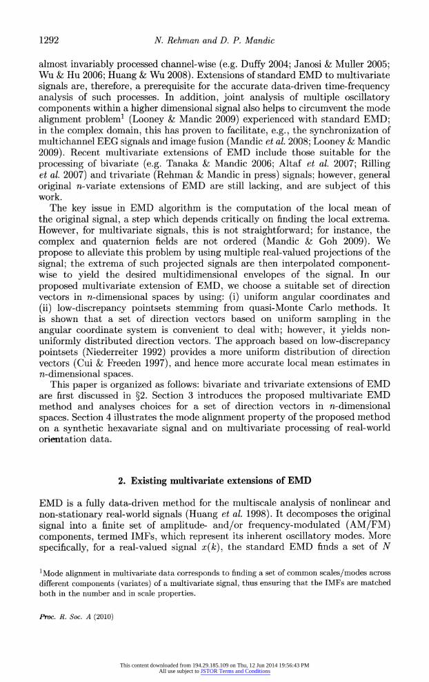
Figure 1. Direction vectors for taking projections of trivariate signals on a two-sphere generated

by using (a) spherical coordinate system and (b) a low-discrepancy Hammersley sequence.

(i) Uniform angular sampling A simple and practically convenient choice for a set of direction vectors

is to employ uniform angular sampling of a unit sphere in an n-dimensional

hyperspherical coordinate system. The resulting set of direction vectors covers the whole (n

? 1) sphere, as shown in figure la for a particular example of a

two-sphere. For the generation of a pointset on an (n ?

1) sphere, consider the n

sphere with centre point C and radius i?, given by

n+l

* = Q)2- (3.1) 3=1

A coordinate system in an n-dimensional Euclidean space can then be defined to serve as a pointset (and the corresponding set of direction vectors) on an

(n ?

1) sphere. Let {0i,02, , 0(n-i)} be the (n ?

1) angular coordinates, then an n-dimensional coordinate system having {^}"=1 as the n coordinates on a unit

(n ?

1) sphere is given by

#i=cos(0i),

x2 = sin(0i) x cos(02),

?3 = sin(0i) x sin(02) x cos(03), (3.2)

xn_i =sin(0i) x x sin(0?_2) x cos(0n_i)

and xn ? sin(0i) x x sin(0n_2) x sin(0n_i).




1296 TV. Rehman and D. P. Mandic

The pointset corresponding to the n-dimensional coordinate system is now very convenient to generate; however, for n > 1, it does not provide a uniform sampling distribution, as illustrated by a higher density of the points when approaching the poles of a two-sphere (figure la).

(ii) Sampling based on low-discrepancy pointsets

We next employ the concept of discrepancy to generate a uniform pointset on an n sphere. Discrepancy can be regarded as a quantitative measure for the irregularity (non-uniformity) of a distribution, and may be used for the

generation of the so-called 'low discrepancy pointset', leading to a more uniform distribution on the n sphere. It belongs to the class of quasi-Monte Carlo methods

(Niederreiter 1992), which are particularly important in numerical integration problems where they ensure smaller error bounds as compared with the standard Monte Carlo methods.4 As the computation of local mean via envelope averaging can be seen as a numerical integration problem, we can use quasi-Monte Carlo

techniques to estimate the local mean within multivariate extension of EMD. This way, the low-discrepancy sequences yield a more uniformly distributed set of direction vectors for generating signal projections and the corresponding signal envelopes ensuring accurate local mean estimates.

A convenient method for generating multidimensional 'low-discrepancy' sequences involves the family of Halton and Hammersley sequences, which are proven to show considerable improvement, in terms of error bounds, over

standard Monte Carlo methods (Niederreiter 1992). Moreover, the set of direction vectors generated by the Hammersley sequence also yields improved generalized discrepancy estimates as compared with other sampling methods, and hence are uniformly distributed on a sphere (Cui & Freeden 1997). To generate the

Hammersley sequence, let x\, x%,..., xn be the first n prime numbers, then the ith sample of a one-dimensional Halton sequence, denoted by rf, is given by

where base-a; representation of i is given by

i=ao + aixx + a2><x2-\-\- as x xs. (3.4)

Starting from i = 0, the ith sample of the Halton sequence then becomes

(r?,rf,...,ff). (3.5) The Hammersley sequence is used when the total number of samples n is

known a priori; in this case, the ith sample within the Hammersley sequence is calculated as

(t/n,ff>ff,...,rf-1). (3.6)

For illustration, figures lb and 2 show, respectively, the pointsets on the surface

of the sphere (two-sphere) and hypersphere (three-sphere) generated by the low

discrepancy Hammersley sequence. Observe that, as desired, the points generated

4Standard Monte Carlo methods, using independent random samples, can also be used to develop

multivariate extensions of EMD. However, this would only result in a probabalistic error bound;

thus, any two applications of the algorithm with similar input and parameters would, in general,

yield different decompositions.





(a) (b)

Y o- ^ : z o.

^x x=xxx*xxxxxx x x Xxxf & *****?"* ? \*f*

^'x^^xx x

xXxW W xx ^ x xx

-Trf w -i^i *

? )

#T*X *xx x

xx*V:

ifx**5 X^Ht<x"xVxx<<JA *x x. x x* xx iXxx x 5 xXx, *}1

xixxx JXxXjxx x* ?x x*^*^ *fx xxxx *jxV; xXxX.?

V"?i ? xxx$ xwJ*

K<>'\ ^_'IT -1^1 w

Figure 2. Direction vectors for taking projections of a quaternion signal (with n = 4 components) on

a unit three-sphere generated by using a low-discrepancy Hammersley sequence. For visualization

purposes, the pointset is plotted on three unit two-spheres, defined, respectively, by (a) WXY,

{b) XYZ and (c) WYZ axes.

by the low-discrepancy method are more uniformly distributed. In figure 2, ideally, the pointset should be plotted on a three-sphere; however, for visualization

purposes, we can only use three two-spheres. The Halton and Hammersley sequence-based pointsets are convenient to

generate; however, their performance may decrease with an increase in the number of dimensions. To alleviate this problem, (t,s) sequences and (t,m,s) nets

(Niederreiter 1992) may be used. Once a suitable set of direction vectors on the n sphere is generated (by using any of the above methods), projections of the

input signal are calculated along this set; the extrema of such projected signals are interpolated component-wise to yield the desired multidimensional envelopes of the signal. The multiple envelope curves, each corresponding to a particular direction vector, are then averaged to obtain the multivariate signal mean.

Consider a sequence of n-dimensional vectors [v(t)}J=1 =

{vi(t), V2(t),..., vn(t)} which represents a multivariate signal with n components, and x?k =

{x?, rz^',..., x^} denoting a set of direction vectors along the directions given by angles 0k = {0f,0|,

... ,0*non

an (n ?

1) sphere. Then, the proposed multivariate extension of EMD suitable for operating on general nonlinear and

non-stationary n-variate time series is summarized in algorithm 2.





Algorithm 2. Multivariate extension of EMD.

1. Choose a suitable pointset for sampling on an (n ?

1) sphere. 2. Calculate a projection, denoted by p6k(t)}J=v of the input signal {v(^)}^L1 along

the direction vector x^, for all k (the whole set of direction vectors), giving

P6k(t)}k=i as ̂ e se^ ?f projections. 3. Find the time instants corresponding to the maxima of the set of projected

signals /*(0lf=r 4. Interpolate [^f*, v(?f*)] to obtain multivariate envelope curves edk(t)}%=1. 5. For a set of K direction vectors, the mean m(t) of the envelope curves is

calculated as

1 K

mW = ^Ee^). (3.7) k=l

6. Extract the 'detail' d(t) using d(t) = x(t) -

m{t). If the 'detail' d(t) fulfills the stoppage criterion for a multivariate IMF, apply the above procedure to

x(t) ?

d(t), otherwise apply it to d(t).

The stoppage criterion for multivariate IMFs is similar to that proposed by Huang et al. (2003), the difference being that the condition for equality of the number of extrema and zero crossings is not imposed, as extrema cannot be

properly defined for multivariate signals (Mandic & Goh 2009).

4. Simulations

Simulations were conducted on both a synthetic signal and a real-world multivariate inertial body motion recording. For all the signals, the low

discrepancy Hammersley sequence was used to generate a set of K ? 512 direction vectors for taking signal projections.

(a) Mode alignment using multivariate IMFs

Similarly to bivariate (Rilling et al. 2007) and trivariate (Rehman & Mandic in press) extensions of EMD, we will now show that the proposed n-variate

extension of EMD has the ability to align 'common scales' present within

multivariate data. Each 'common scale' is manifested in the common oscillatory modes in all the variates within an n-variate IMF. Such mode alignment property

helps to make use of similar scales in different data sources, and hence, can

be used for data fusion purposes (Mandic et al. 2008). To illustrate the mode

alignment property of the proposed method, we analysed a synthetic hexavariate

time series; each component (variate), shown in the top row of figure 3 (denoted by U, V, W,X, Y and Z), was constructed from a set of four sinusoids. One

sinusoid was made common to all the components, whereas the remaining three

sinusoidal components were combined so that the resulting signal had a common





vW(\w^ xVVKiWWl ^

-5 J-.-1 J-1-1 J-.-1 J-.-1 J-?-1 J- -

5 -i-1 i-1 -1-1 -1-1 -I-1 "j

llllllllllllllUlllllllllilll llllllllllllllllllilllllll lllillllllllllllllllilllllllll ^,o "IhIhI

Vi "BBl

W{??~Xi IBB

Yi-Z]

5 -i-1 -i-1 -I-1 -I-1 i-1 -i

-5 "I-.-1 J-.-1 J-.-1 J-.-1 J-.-1 J-.

5 i-1 -i-1 -i-1 -j-1 -i-1 i

0 500 1000 0 500 1000 0 500 1000 0 500 1000 0 500 1000 0 500 1000

time index time index time index time index time index time index

Figure 3. Decomposition of a synthetic multivariate signal (U, V, W, X, V, Z) exhibiting multiple frequency modes (with f\ = 2 Hz, = 8 Hz, fa = 16 Hz and fa = 32 Hz) via the proposed multivariate EMD algorithm. Each IMF carries a single frequency mode, illustrating the alignment of common

scales within different components of a multivariate signal.

frequency mode in each UVWY, UVX and UWXZ components. The proposed n-variate EMD extension was then applied to the resulting hexavariate signal yielding multiple IMFs, as shown in figure 3. Observe that the sinusoid common to all the components of the input is the third IMF, whereas the remaining three

frequency modes were also accurately extracted in the respective IMFs. Notice the similar separability of the tones as with standard EMD; for more detail, see

Rilling & Flandrin (2008). Such mode alignment cannot be achieved by the real valued EMD applied component-wise, as it generally does not yield the same

number of IMFs per component.





^ " ^^^^^^^^^^^ ^ " -^^^^^^^^^^^ ,00^ ^? 10?^-?b~-^00

y -100 -,0? x Y 0 -200 X

IMF3 IMF3

l00~ <=^^^^^^^> ,00^ ^^^^^^^^^^^^^

y -so _4o _2? x ?

y -50 _5? x? IMF4 IMF4

^^^^^ y -50 -100 x? Y "20 "50 X

IMF5 IMF5 40-1 20 -.

y~10 -2o_2o x? y ~20 -20 x?

residue residue

50-, 100 ^ ^^~)

40 ^^V^^^Jo^^0 5??5 70^^^^?-^r^o ^? fs\ 4U 65 ^??-on -60

Y -20 _80 "60 X y 60 _100

"80 X

Figure 4. A real-world hexavariate orientation signal and its decomposition via the proposed multivariate EMD algorithm. Trivariate orientation signals corresponding to the (a) left-hand

movement, and (b) the left ankle movement, are shown in the top row, with selected IMFs below

depicting the common rotational modes.

(b) Rotational modes extraction from real-world signals

To illustrate the ability of the proposed method to extract common modes within multivariate real-world signals, we next considered body motion data recorded in a Tai Chi sequence. The data were captured using two inertial three-dimensional sensors attached to the left hand and the left ankle; these were combined to form a single hexavariate signal. The common rotational modes were found within multiple hexavariate IMFs, and the components corresponding to the hand and the ankle were plotted separately as three dimensional plots in figure 4. Observe that each such IMF represents a unique rotational mode embedded within the original trivariate signal. Unlike when

applying the trivariate EMD method separately on each three-dimensional signal,





our proposed method guarantees the extraction of common rotational modes, as the direct analysis of a hexavariate signal results in matched IMFs (both in number and in frequency scale).

5. Conclusions

An extension of EMD has been proposed to cater for a general class of n-variate

signals. The critical step of envelope interpolation is performed by taking projections of the multivariate signal along multiple directions on an n sphere. In addition, the use of low discrepancy pointset gives uniformly distributed direction vectors on an n sphere and makes the resulting method accurate and

computationally efficient. It has been shown that the proposed method has the ability to extract common rotational modes across the signal components,

making it suitable, for example, for fusion of information from multiple sources. Simulations on synthetic and real-world hexavariate data support the analysis.

References

Altaf, M. U., Gautama, T., Tanaka, T. & Mandic, D. P. 2007 Rotation invariant complex

empirical mode decomposition. In Proc. IEEE Int. Conf. on Acoustics, Speech, Signal Processing,

Honolulu, HI, April 2007, pp. 1009-1012.

Cui, J. & Freeden, W. 1997 Equidistribution on the sphere. SI AM J. Sci. Comput. 18, 595-609.

(doi: 10.1137/S1064827595281344) Duffy, D. J. 2004 The application of Hilbert-Huang transforms to meteorological datasets.

J. Atmos. Ocean. Tech. 21, 599-611. (doi:10.1175/1520-0426(2004)02K0599:TAOHTT> 2.0.CO;2)

Gautama, T., Mandic, D. P. & Hulle, M. M. V. 2004 The delay vector variance method for

detecting determinism and nonlinearity in time series. Physica D 190, 167-176. (doi: 10.1016/

j.physd.2003.11.001)

Huang, N. E. & Shen, S. S. P. (eds) 2005 Hilbert-Huang transform and its applications. Singapore: World Scientific.

Huang, N. E., Shen, Z., Long, S., Wu, M., Shih, H., Zheng, Q., Yen, N., Tung, C. & Liu, H. 1998

The empirical mode decomposition and Hilbert spectrum for non-linear and non-stationary time

series analysis. Proc. R. Soc. Lond. A 454, 903-995. (doi:10.1098/rspa.l998.0193) Huang, N. E., Wu, M., Long, S., Shen, S., Qu, W., Gloersen, P. & Fan, K. 2003 A confidence limit

for the empirical mode decomposition and Hilbert spectral analysis. Proc. R. Soc. Lond. A 459, 2317-2345. (doi: 10.1098/rspa.2003.1123)

Huang, N. E. & Wu, Z. 2008 A review on Hilbert-Huang transform: method and its applications to geophysical studies. Rev. Geophys. 46, RG2006. (doi:10.1029/2007RG000228)

Janosi, I. M. & Muller, R. 2005 Empirical mode decomposition and correlation properties of long

daily ozone records. Phys. Rev. E 71, 056126. (doi:10.1103/PhysRevE.71.056126) Lin, S., Tung, P. & Huang, N. E. 2009 Data analysis using a combination of independent

component analysis and empirical mode decomposition. Phys. Rev. E 79, 066705. (doi: 10.1103/

PhysRevE.79.066705) Looney, D. & Mandic, D. P. 2009 Multi-scale image fusion using complex extensions of EMD. IEEE

T. Signal Process. 57, 1626-1630.

Mandic, D. P., Golz, M., Kuh, A., Obradoric, D. & Tanaka, T. (eds) 2008 Signal processing

techniques for knowledge extraction and information fusion. Berlin, Germany: Springer. Mandic, D. P. & Goh, V. S. L. 2009 Complex valued non-linear adaptive filters: noncircularity,

widely linear neural models. New York, NY: Wiley.





Niederreiter, H. 1992 Random number generation and quasi-Monte Carlo methods. Philadelphia, PA: Society for Industrial and Applied Mathematics.

Rehman, N. & Mandic, D. P. In press. Empirical mode decomposition for trivariate signals. IEEE

T. Signal Process.

Rilling, G. & Flandrin, P. 2008 One or two frequencies? The empirical mode decomposition answers.

IEEE Trans. Signal Process. 56, 85-95.

Rilling, G., Flandrin, P., Goncalves, P. & Lilly, J. M. 2007 Bivariate empirical mode decomposition. IEEE Signal Process. Lett. 14, 936-939.

Tanaka, T. & Mandic, D. P. 2006 Complex empirical mode decomposition. IEEE Signal Process.

Lett. 14, 101-104.

Wu, M. & Hu, C. 2006 Empirical mode decomposition and synchrogram approach to

cardiorespiratory synchronization. Phys. Rev. E 73, 051917. (doi:10.1103/PhysRevE.73.051917)




Multivariate empirical mode decomposition

Documents

Transcript of Multivariate empirical mode decomposition