Multivariate Data Analysis

Susan Holmes ©http://www-stat.stanford.edu/˜susan/

Bio-X and Statistics

IMA Workshop, October, 2013

ABabcdfghiejkl..... ..... ..... . ..................... ..................... ..................... ..... ..... . ..... ..... ..... .

you do not really understand something unless you canexplain it to your grandmother -- Albert Einstein

I am your grandmother .........

..... ..... ..... . ..................... ..................... ..................... ..... ..... . ..... ..... ..... .

you do not really understand something unless you canexplain it to your grandmother -- Albert EinsteinI am your grandmother .........

..... ..... ..... . ..................... ..................... ..................... ..... ..... . ..... ..... ..... .

What are multivariate data ?

Simplest format: matrices:If we have measured 10,000 genes on hundreds of patientsand all the genes are independent, we can't do better thananalyze each gene's behavior by using histograms or boxplots, looking at the means, medians, variances and other `onedimensional statistics'. However if some of the genes areacting together, either that they are positively correlated orthat they inhibit each other, we will miss a lot of importantinformation by slicing the data up into those column vectorsand studying them separately. Thus important connectionsbetween genes are only available to us if we consider thedata as a whole. We start by giving a few examples of datathat we encounter. ..... ..... ..... . ..................... ..................... ..................... ..... ..... . ..... ..... ..... .

▶ Athletes, performances in the decathlon.

100 long poid haut 400 110 disq perc jave 15001 11.25 7.43 15.48 2.27 48.90 15.13 49.28 4.7 61.32 268.952 10.87 7.45 14.97 1.97 47.71 14.46 44.36 5.1 61.76 273.023 11.18 7.44 14.20 1.97 48.29 14.81 43.66 5.2 64.16 263.204 10.62 7.38 15.02 2.03 49.06 14.72 44.80 4.9 64.04 285.115 11.02 7.43 12.92 1.97 47.44 14.40 41.20 5.2 57.46 256.64

▶ Clinical measurements (diabetes data).relwt glufast glutest steady insulin Group

1 0.81 80 356 124 55 33 0.94 105 319 143 105 35 1.00 90 323 240 143 37 0.91 100 350 221 119 39 0.99 97 379 142 98 3

▶ OTU read counts:469478 208196 378462 265971 570812

EKCM1.489478 0 0 2 0 0EKCM7.489464 0 0 2 0 2EKBM2.489466 0 0 12 0 0..... ..... ..... . ..................... ..................... ..................... ..... ..... . ..... ..... ..... .

PTCM3.489508 0 0 14 0 0EKCF2.489571 0 0 4 0 0

▶ RNA-seq, transcriptomic:

FBgn0000017 FBgn0000018 FBgn0000022 FBgn0000024 FBgn0000028 FBgn0000032untreated1 4664 583 0 10 0 1446untreated2 8714 761 1 11 1 1713untreated4 3150 310 0 3 0 672treated1 6205 722 0 10 0 1698treated3 3334 308 0 5 1 757

▶ Mass spec:Samples × Features.

mz 129.9816 72.08144 151.6255 142.0349 169.0413 186.0355KOGCHUM1 60515 181495 0 196526 25500 51504.4012WTGCHUM1 252579 54697 412 487800 48775 130491.1538WTGCHUM2 187859 56318 46425 454226 45626 100845.0179..... ..... ..... . ..................... ..................... ..................... ..... ..... . ..... ..... ..... .

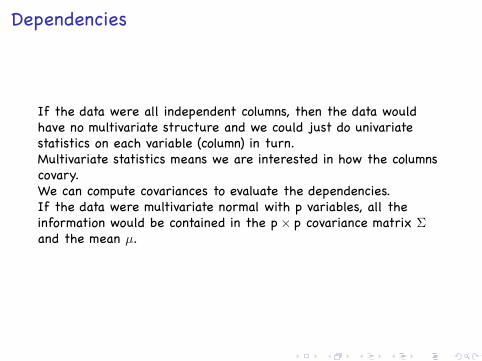
Dependencies

If the data were all independent columns, then the data wouldhave no multivariate structure and we could just do univariatestatistics on each variable (column) in turn.Multivariate statistics means we are interested in how the columnscovary.We can compute covariances to evaluate the dependencies.If the data were multivariate normal with p variables, all theinformation would be contained in the p× p covariance matrix Σand the mean µ.

..... ..... ..... . ..................... ..................... ..................... ..... ..... . ..... ..... ..... .

Parametric Multivariate Normal

..... ..... ..... . ..................... ..................... ..................... ..... ..... . ..... ..... ..... .

Modern Statistics: Non parametric, multivariate

▶ Exploratory Analyses: Hypotheses generating.▶ Projection Methods (new coordinates)▶ Principal Component Analysis▶ Principal Coordinate Analysis-Multidimensional Scaling

(PCO,MDS)▶ Correspondence Analysis▶ Discriminant Analysis▶ Tree based methods▶ Phylogenetic Trees▶ Clustering Trees▶ Decision Trees

▶ Confirmatory Analyses: Hypothesis verification.▶ Permutation tests (Monte Carlo).▶ Bootstrap (Monte Carlo).▶ Bayesian nonparametrics (Monte Carlo).

..... ..... ..... . ..................... ..................... ..................... ..... ..... . ..... ..... ..... .

Modern Methods: Robust Methods

VarianceVariability of one continuous variable −→ the variance.NOT ROBUST, low breakdown.Solution: Take ranks, clumps, logs, or trimming the data.

..... ..... ..... . ..................... ..................... ..................... ..... ..... . ..... ..... ..... .

Part I

EDA: Exploratory Data Analysis

Data CheckingHypothesis Generating

..... ..... ..... . ..................... ..................... ..................... ..... ..... . ..... ..... ..... .

Discovery by Visualization d = 0.02

●

●

●

● ●

●

●

●

●

●

●

●

●

●

●

●

●

●

●

●

●

●

●

●

●

●

●

● 1

2

3

..... ..... ..... . ..................... ..................... ..................... ..... ..... . ..... ..... ..... .

Basic Visualization Tools

▶ Boxplots, barplots.▶ Scatterplots of projected data.▶ Scatterplots with binning variable▶ Hierarchical Clustering, heatmaps, Phylogenies.▶ Combination of Phylogenetic Trees and data.

..... ..... ..... . ..................... ..................... ..................... ..... ..... . ..... ..... ..... .

Iterative Structuration (Tukey, 1977)

..... ..... ..... . ..................... ..................... ..................... ..... ..... . ..... ..... ..... .

One table methods: PCA, MDS, PCoA, CA, .....

. DATA

means variances

k?

Change of Data

end

Choice

Choice

variables

observations

All based on the principle of finding the largest axis ofinertia/variability.

New Variables/coordinates from old or distancesBest Projection Directions??

..... ..... ..... . ..................... ..................... ..................... ..... ..... . ..... ..... ..... .

..... ..... ..... . ..................... ..................... ..................... ..... ..... . ..... ..... ..... .

..... ..... ..... . ..................... ..................... ..................... ..... ..... . ..... ..... ..... .

PCA procedure

. DATA

means variances

k?

Change of Data

end

Choice

Choice

variables

observations

All based on the principle of finding the largest axis ofinertia/variability.

New Variables/coordinates from old or distancesBest Projection Directions because they explain the most variance.

..... ..... ..... . ..................... ..................... ..................... ..... ..... . ..... ..... ..... .

Our first task is often to rescale the data so that all thevariables, or columns of the matrix have the same standarddeviation, this will put all the variables on the same footing.We also make sure that the means of all columns are zero,this is called centering. After that we will try to simplify thedata by doing what we call rank reduction, we'll explain thisconcept from several different perspectives. A favorite toolfor simplifying the data is called Principal Component Analysis(abbreviated PCA).

..... ..... ..... . ..................... ..................... ..................... ..... ..... . ..... ..... ..... .

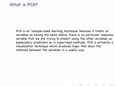
What is PCA?

PCA is an `unsupervised learning technique' because it treats allvariables as having the same status, there is no particular responsevariable that we are trying to predict using the other variables asexplanatory predictors as in supervised methods. PCA is primarily avisualization technique which produces maps that show therelations between the variables in a useful way.

..... ..... ..... . ..................... ..................... ..................... ..... ..... . ..... ..... ..... .

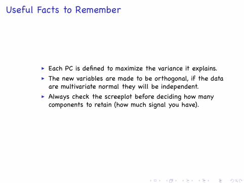
Useful Facts to Remember

▶ Each PC is defined to maximize the variance it explains.▶ The new variables are made to be orthogonal, if the data

are multivariate normal they will be independent.▶ Always check the screeplot before deciding how many

components to retain (how much signal you have).

..... ..... ..... . ..................... ..................... ..................... ..... ..... . ..... ..... ..... .

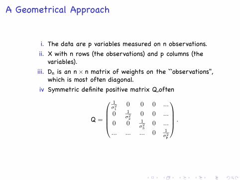
A Geometrical Approach

i. The data are p variables measured on n observations.ii. X with n rows (the observations) and p columns (the

variables).iii. Dn is an n× n matrix of weights on the ``observations'',

which is most often diagonal.iv Symmetric definite positive matrix Q,often

Q =

1σ21

0 0 0 ...

0 1σ22

0 0 ...

0 0 1σ23

0 ...

... ... ... 0 1σ2

p

.

..... ..... ..... . ..................... ..................... ..................... ..... ..... . ..... ..... ..... .

Euclidean Spaces

These three matrices form the essential ``triplet" (X,Q,D) defininga multivariate data analysis.Q and D define geometries or inner products in Rp and Rn,respectively, through

xtQy =< x, y >Q x, y ∈ Rp

xtDy =< x, y >D x, y ∈ Rn.

..... ..... ..... . ..................... ..................... ..................... ..... ..... . ..... ..... ..... .

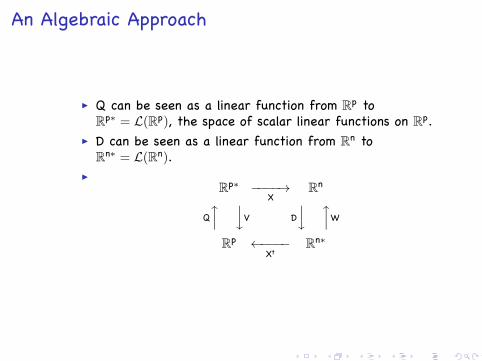
An Algebraic Approach

▶ Q can be seen as a linear function from Rp toRp∗ = L(Rp), the space of scalar linear functions on Rp.

▶ D can be seen as a linear function from Rn toRn∗ = L(Rn).

▶Rp∗ −−−−→

XRn

Qx yV D

y xW

Rp ←−−−−Xt

Rn∗

..... ..... ..... . ..................... ..................... ..................... ..... ..... . ..... ..... ..... .

An Algebraic Approach

Rp∗ −−−−→X

Rn

Qx yV D

y xW

Rp ←−−−−Xt

Rn∗

Duality diagrami. Eigendecomposition of XtDXQ = VQii. Eigendecomposition of XQXtD = WDiii. Transition Formulae.

..... ..... ..... . ..................... ..................... ..................... ..... ..... . ..... ..... ..... .

Notes

(1) Suppose we have data and inner products defined by Q and D :

(x, y) ∈ Rp × Rp 7−→ xtQy = < x, y >Q∈ R

(x, y) ∈ Rn × Rn 7−→ xtDy = < x, y >D∈ R.

||x||2Q =< x, x >Q=

p∑j=1

qj(x.j)2 ||x||2D =< x, x >D=

p∑j=1

pi(xi.)2

(2) We say an operator O is B-symmetric if < x,Oy >B=< Ox, y >B,or equivalently BO = OtB.The duality diagram is equivalent to (X,Q,D) such that X is n× p .Escoufier (1977) defined as XQXtD = WD and XtDXQ = VQ as thecharacteristic operators of the diagram.

..... ..... ..... . ..................... ..................... ..................... ..... ..... . ..... ..... ..... .

(3) V = XtDX will be the variance-covariance matrix, if X iscentered with regards to D (X′D1n = 0).

..... ..... ..... . ..................... ..................... ..................... ..... ..... . ..... ..... ..... .

Transposable Data

There is an important symmetry between the rows and columns ofX in the diagram, and one can imagine situations where the role ofobservation or variable is not uniquely defined. For instance inmicroarray studies the genes can be considered either as variablesor observations. This makes sense in many contemporary situationswhich evade the more classical notion of n observations seen as arandom sample of a population. It is certainly not the case thatthe 9,000 species are a random sample of bacteria since theseprobes try to be an exhaustive set.

..... ..... ..... . ..................... ..................... ..................... ..... ..... . ..... ..... ..... .

Two Dual Geometries

..... ..... ..... . ..................... ..................... ..................... ..... ..... . ..... ..... ..... .

Properties of the Diagram

Rank of the diagram: X,Xt,VQ and WD all have the same rank.For Q and D symmetric matrices, VQ and WD are diagonalisableand have the same eigenvalues.

λ1 ≥ λ2 ≥ λ3 ≥ . . . ≥ λr ≥ 0 ≥ · · · ≥ 0.

Eigendecomposition of the diagram: VQ is Q symmetric, thus wecan find Z such that

VQZ = ZΛ,ZtQZ = Ip, where Λ = diag(λ1, λ2, . . . , λp). (1)

..... ..... ..... . ..................... ..................... ..................... ..... ..... . ..... ..... ..... .

Practical Computations

Cholesky decompositions of Q and D, (symmetric and positivedefinite) HtH = Q and KtK = D.Use the singular value decomposition of KXH:

KXH = USTt, with TtT = Ip,UtU = In,S diagonal.

Then Z = (H−1)tT satisfies

VQZ = ZΛ,ZtQZ = Ip

with Λ = S2.The renormalized columns of Z, A = SZ are called the principalaxes and satisfy:

AtQA = Λ.

..... ..... ..... . ..................... ..................... ..................... ..... ..... . ..... ..... ..... .

Practical Computations

Similarly, we can define L = K−1U that satisfies

WDL = LΛ, LtDL = In, where Λ = diag(λ1, λ2, . . . , λr, 0, . . . , 0). (2)

C = LS is usually called the matrix of principal components. It isnormed so that

CtDC = Λ.

..... ..... ..... . ..................... ..................... ..................... ..... ..... . ..... ..... ..... .

Transition Formulæ:

Of the four matrices Z,A, L and C we only have to compute one, allothers are obtained by the transition formulæ provided by theduality property of the diagram:

XQZ = LS = C XtDL = ZS = A

..... ..... ..... . ..................... ..................... ..................... ..... ..... . ..... ..... ..... .

General Features

1. Inertia : Trace(VQ) = Trace(WD)(inertia in the sense of Huyghens inertia formula for instance).Huygens, C. (1657),

n∑i=1

pid2(xi, a)

Inertia with regards to a point a of a cloud of pi-weighted points.PCA with Q = Ip, D = 1

nIn, and the variables are centered, theinertia is the sum of the variances of all the variables.If the variables are standardized (Q is the diagonal matrix ofinverse variances), then the inertia is the number of variables p.For correspondence analysis the inertia is the Chi-squared statistic.

..... ..... ..... . ..................... ..................... ..................... ..... ..... . ..... ..... ..... .

Ordination Methods

Many discrete measurements −→ Gradients.Data from 2005 U.S. House of Representatives roll call votes. Wefurther restricted our analysis to the 401 Representatives thatvoted on at least 90% of the roll calls (220 Republicans, 180Democrats and 1 Independent) leading to a 401× 669 matrix V ofvoting data.

..... ..... ..... . ..................... ..................... ..................... ..... ..... . ..... ..... ..... .

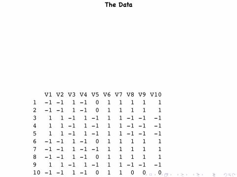
The Data

V1 V2 V3 V4 V5 V6 V7 V8 V9 V101 -1 -1 1 -1 0 1 1 1 1 12 -1 -1 1 -1 0 1 1 1 1 13 1 1 -1 1 -1 1 1 -1 -1 -14 1 1 -1 1 -1 1 1 -1 -1 -15 1 1 -1 1 -1 1 1 -1 -1 -16 -1 -1 1 -1 0 1 1 1 1 17 -1 -1 1 -1 -1 1 1 1 1 18 -1 -1 1 -1 0 1 1 1 1 19 1 1 -1 1 -1 1 1 -1 -1 -110 -1 -1 1 -1 0 1 1 0 0 0..... ..... ..... . ..................... ..................... ..................... ..... ..... . ..... ..... ..... .

!0.1!0.05

00.05

0.1!0.2

!0.1

0

0.1

0.2

!0.2

!0.15

!0.1

!0.05

0

0.05

0.1

0.15

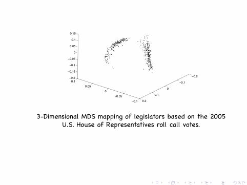
3-Dimensional MDS mapping of legislators based on the 2005U.S. House of Representatives roll call votes.

..... ..... ..... . ..................... ..................... ..................... ..... ..... . ..... ..... ..... .

!0.1!0.05

00.05

0.1!0.2

!0.1

0

0.1

0.2

!0.2

!0.15

!0.1

!0.05

0

0.05

0.1

0.15

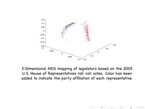
3-Dimensional MDS mapping of legislators based on the 2005U.S. House of Representatives roll call votes. Color has beenadded to indicate the party affiliation of each representative.

..... ..... ..... . ..................... ..................... ..................... ..... ..... . ..... ..... ..... .

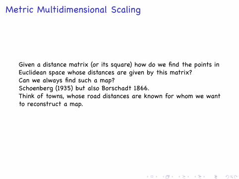
Metric Multidimensional Scaling

Given a distance matrix (or its square) how do we find the points inEuclidean space whose distances are given by this matrix?Can we always find such a map?Schoenberg (1935) but also Borschadt 1866.Think of towns, whose road distances are known for whom we wantto reconstruct a map.

..... ..... ..... . ..................... ..................... ..................... ..... ..... . ..... ..... ..... .

Decomposition of DistancesIf we started with original data in Rp that are not centered: Y,apply the centering matrix

X = HY, with H = (I− 1

n11′), and 1′ = (1, 1, 1 . . . , 1)

Call B = XX′, if D(2) is the matrix of squared distances betweenrows of X in the euclidean coordinates, we can show that

−1

2HD(2)H = B

We can go backwards from a matrix D to X by taking theeigendecomposition of B in much the same way that PCA providesthe best rank r approximation for data by taking the singular valuedecomposition of X, or the eigendecomposition of XX′.

X(r) = US(r)V′ with S(r) =

s1 0 0 0 ...0 s2 0 0 ...0 0 ... ... ...0 0 ... sr ...... ... ... 0 0

..... ..... ..... . ..................... ..................... ..................... ..... ..... . ..... ..... ..... .

Multidimensional Scaling also called PCoA

Simple classical multidimensional scaling.▶ Square D elementwise D(2) = D2.▶ Compute −1

2 HD2H = B.▶ Diagonalize B to find the principal coordinates.

Important: What D to use.

..... ..... ..... . ..................... ..................... ..................... ..... ..... . ..... ..... ..... .

Distances, Similarities, DissimilaritiesDistances:

▶ Euclidean▶ Chisquare

Chisquare(exp, obs) =∑

j

(expj − obsj)2

expj

▶ Hamming/L1▶ DNA distances (dist.dna in ape)

Similarity Indices:▶ Confusion (cognitive psychology).▶ Matching coefficient

nb of matching attrsnb of attrs =

f11 + f00f11 + f00 + f10 + f01

▶ Jaccard Similarity Index.

JA + B− J =

aa + b + c

See versions in vegan and ade4...... ..... ..... . ..................... ..................... ..................... ..... ..... . ..... ..... ..... .

Projection Methods

Project Various Factors as class labels onto thefirst few coordinates (components, factors,...).Projection of supplementary group centers (means)and ellipses of variation (variance) as in thefunction s.class in the ade4 package Example:Explore batch effects in the laboratory methods usedto generate the data. See quality of replicates

..... ..... ..... . ..................... ..................... ..................... ..... ..... . ..... ..... ..... .

d = 0.5

mLS.73.75.A mLS.73.76.B

mMS.43.26.A mMS.43.27.B

mMS.43.27.B.11

mSS.72.57.2 mSS.72.57.3rep mSS.72.77.3 mSS.72.74.4rep mSS.72.77.3.12

..... ..... ..... . ..................... ..................... ..................... ..... ..... . ..... ..... ..... .

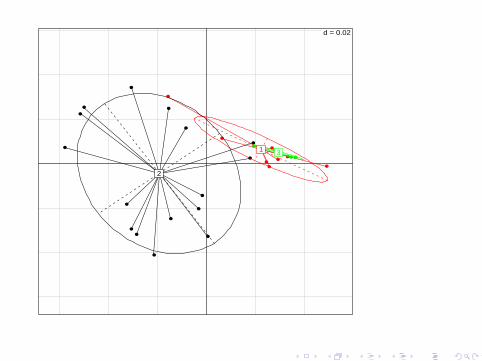
Projection of a categorical variable on a PCA

In the case of PCA: The ellipses are computed using the means,variances and covariance of each group of points on both axes, andare drawn with these parameters: the center of the ellipse iscentered on the means, its width and height are given by thevariances, and the covariance sets the slope of the main axis ofthe ellipse.

..... ..... ..... . ..................... ..................... ..................... ..... ..... . ..... ..... ..... .

First two batches (in black and red)(although both balanced with regards to IBS and healthy rats)were extremely different in variability and overall multivariatelocation. Batches were done different days with different sets of

arrays.

d = 0.02

●

●

●

● ●

●

●

●

●

●

●

●

●

●

●

●

●

●

●

●

●

●

●

●

●

●

●

●

1

2

Two Batches of Arrays−First Plane

..... ..... ..... . ..................... ..................... ..................... ..... ..... . ..... ..... ..... .

A third batch was generated with the same arrays as batch 2 butthe same experimental protocol as batch 1. The third groupfaithfully overlaps with batch 1 thus showing that the batch effectwas not due to a difference in arrays but to the experimentalprotocol. This shows the utility of PCA in quality control.

d = 0.02

●

●

●

● ●

●

●

●

●

●

●

●

●

●

●

●

●

●

●

●

●

●

●

●

●

●

●

● 1

2

3

..... ..... ..... . ..................... ..................... ..................... ..... ..... . ..... ..... ..... .

d = 0.02

●

●

●

● ●

●

●

●

●

●

●

●

●

●

●

●

●

●

●

●

●

●

●

●

●

●

●

● 1

2

3

..... ..... ..... . ..................... ..................... ..................... ..... ..... . ..... ..... ..... .

Chisquare: Aims and Relevant Data

What is a contingency table?An example (thanks to the xkcd blag):

black blue green grey orange purple whitequiet 27700 21500 21400 8750 12200 8210 25100

angry 29700 15300 17400 7520 10400 7100 17300clever 16500 12700 13200 4950 6930 4160 14200

depressed 14800 9570 9830 1470 3300 1020 12700happy 193000 83100 87300 19200 42200 26100 91500lively 18400 12500 13500 6590 6210 4880 14800

perplexed 1100 713 801 189 233 152 1090virtuous 1790 802 1020 200 247 173 1650

..... ..... ..... . ..................... ..................... ..................... ..... ..... . ..... ..... ..... .

Correspondence analysis (CA, also called homogeneity analysisand reciprocal averaging), can be used to analyse severaltypes of multivariate data. All involve some categoricalvariables. Here are some examples of the type of data thatcan be decomposed using this method:

▶ Contingency Tables (cross between two categoricalvariables)

▶ Multiple Contingency Tables (cross between severalcategorical variables).

▶ Binary tables obtained by cutting continuous variablesinto classes and then recoding both these variables andany extra categorical variables into 0/1 tables, 1 indicatingpresence in that class. So for instance a continuousvariable cut into three classes will provide three newbinary variables of which only one can take the value 1for any given observation.

For a complete treatment, see the paper: MultivariateData Analysis: the French Way[6] (see my homepagefor papers).

..... ..... ..... . ..................... ..................... ..................... ..... ..... . ..... ..... ..... .

To first approximation, correspondence analysis can beunderstood as an extension of principal components analysis(PCA) where the variance in PCA is replaced by an inertiaproportional to the χ2 distance of the table fromindependence. CA decomposes this measure of departure fromindependence along axes that are orthogonal according to theχ2 inner product.

..... ..... ..... . ..................... ..................... ..................... ..... ..... . ..... ..... ..... .

Plato's works

In statistics the most commonplace use of Correspondence Analysisis in ordination or seriation, that is , the search for a hiddengradient in contingency tables. As an example we take dataanalysed by Cox and Brandwood who wanted to seriate Plato'sworks using the proportion of sentence endings in a given book,with a given stress pattern. We propose the use of correspondenceanalysis on the table of frequencies of sentence endings.

..... ..... ..... . ..................... ..................... ..................... ..... ..... . ..... ..... ..... .

The first 10 profiles (as percentages) look as follows:Rep Laws Crit Phil Pol Soph Tim

UUUUU 1.1 2.4 3.3 2.5 1.7 2.8 2.4-UUUU 1.6 3.8 2.0 2.8 2.5 3.6 3.9U-UUU 1.7 1.9 2.0 2.1 3.1 3.4 6.0UU-UU 1.9 2.6 1.3 2.6 2.6 2.6 1.8UUU-U 2.1 3.0 6.7 4.0 3.3 2.4 3.4UUUU- 2.0 3.8 4.0 4.8 2.9 2.5 3.5--UUU 2.1 2.7 3.3 4.3 3.3 3.3 3.4-U-UU 2.2 1.8 2.0 1.5 2.3 4.0 3.4-UU-U 2.8 0.6 1.3 0.7 0.4 2.1 1.7-UUU- 4.6 8.8 6.0 6.5 4.0 2.3 3.3.......etc (there are 32 rows in all)The eigenvalue decomposition (called the scree plot) of thechisquare distance matrix shows that two axes out of apossible 6 (the matrix is of rank 6) will provide a summary of85% of the departure from independence, this suggests that aplanar representation will provide a good visual summary ofthe data.

Eigenvalue inertia % cumulative %1 0.09170 68.96 68.962 0.02120 15.94 84.90..... ..... ..... . ..................... ..................... ..................... ..... ..... . ..... ..... ..... .

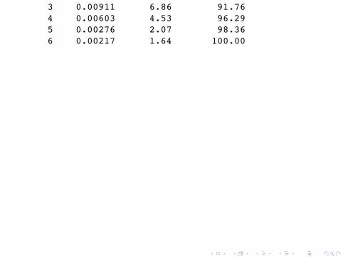
3 0.00911 6.86 91.764 0.00603 4.53 96.295 0.00276 2.07 98.366 0.00217 1.64 100.00

..... ..... ..... . ..................... ..................... ..................... ..... ..... . ..... ..... ..... .

Tim

Laws Rep

Soph

Phil

PolCrit

Axis #1: 69%

Ax

is #

2:

16

%

-0.2 0.0 0.2 0.4

0.0

-0.2

-0.3

-0.1

0.1

Correspondence Analysis of Plato's Works

We can see from the plot that there is a seriation that as in..... ..... ..... . ..................... ..................... ..................... ..... ..... . ..... ..... ..... .

most cases follows a parabola,horseshoe or arch from Laws onone extreme being the latest work and Republica being theearliest among those studied.

..... ..... ..... . ..................... ..................... ..................... ..... ..... . ..... ..... ..... .

We will also consider `multiple contingency tables' where more thantwo categorical variables are compared.

, , Sex = MaleEye

Hair Brown Blue Hazel GreenBlack 32 11 10 3Brown 53 50 25 15Red 10 10 7 7Blond 3 30 5 8

, , Sex = FemaleEye

Hair Brown Blue Hazel GreenBlack 36 9 5 2Brown 66 34 29 14Red 16 7 7 7Blond 4 64 5 8

..... ..... ..... . ..................... ..................... ..................... ..... ..... . ..... ..... ..... .

> HairColor=HairEyeColor[,,2]> chisq.test(HairColor)

Pearson's Chi-squared test

data: HairColorX-squared = 106.6637, df = 9, p-value < 2.2e-16

Warning message:In chisq.test(HairColor) : Chi-squared approximation may be incorrect

..... ..... ..... . ..................... ..................... ..................... ..... ..... . ..... ..... ..... .

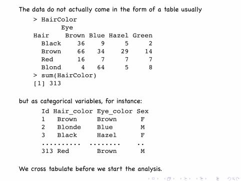
The data do not actually come in the form of a table usually> HairColor

EyeHair Brown Blue Hazel Green

Black 36 9 5 2Brown 66 34 29 14Red 16 7 7 7Blond 4 64 5 8

> sum(HairColor)[1] 313

but as categorical variables, for instance:Id Hair_color Eye_color Sex1 Brown Brown F2 Blonde Blue M3 Black Hazel F.......... ........ ..313 Red Brown M

We cross tabulate before we start the analysis...... ..... ..... . ..................... ..................... ..................... ..... ..... . ..... ..... ..... .

> res.coa=dudi.coa(HairColor)> s.label(res.coa$c1,boxes=F)> s.label(res.coa$li,add.plot=TRUE)

d = 0.5

Brown

Blue

Hazel

Green

Black

Brown

Red

Blond

..... ..... ..... . ..................... ..................... ..................... ..... ..... . ..... ..... ..... .

Independence

If we are comparing two categorical variables, (hair color, eyecolor), (color, emotion), the simplest possible model is that ofindependence in which case the counts in the table would obeyapproximately the margin products identity for a I× J contingencytable with a total sample size of n =

∑Ii=1

∑Jj=1 nij = n··.

nij.=

ni·

nn·jn n

can also be written: N .= cr′n, where

c =1

nN1m and r′ = 1nN′1p

The departure from independence is measured by the χ2 statistic

X 2 =∑i,j

[(nij − ni·

nn·jn n)2

ni·n·jn2 n

]

..... ..... ..... . ..................... ..................... ..................... ..... ..... . ..... ..... ..... .

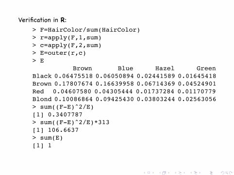
Verification in R:> F=HairColor/sum(HairColor)> r=apply(F,1,sum)> c=apply(F,2,sum)> E=outer(r,c)> E

Brown Blue Hazel GreenBlack 0.06475518 0.06050894 0.02441589 0.01645418Brown 0.17807674 0.16639958 0.06714369 0.04524901Red 0.04607580 0.04305444 0.01737284 0.01170779Blond 0.10086864 0.09425430 0.03803244 0.02563056> sum((F-E)^2/E)[1] 0.3407787> sum((F-E)^2/E)*313[1] 106.6637> sum(E)[1] 1

..... ..... ..... . ..................... ..................... ..................... ..... ..... . ..... ..... ..... .

Matrix decomposition and χ2 distances

To compute the distance between profiles, each column isreweighted by the inverse of its sum, this gives the χ2 distancebetween row profiles.

X 2 = n trace ((F− rc′)′Dr−1(F− rc′)Dc

−1)

= trace (A′A) where A = D−1√r(F− rc′)D−1√

c

The latter decomposition shows a justification for choosing thematrix A as a natural square root. W = A′A is in a sense thecharacteristic matrix-operator of the analysis, in the same way thecovariance or correlation matrices are those of principalcomponents analysis.

..... ..... ..... . ..................... ..................... ..................... ..... ..... . ..... ..... ..... .

Correspondence analysis decomposes the matrix W: itseigenvectors give the axes that account for the largest part of thedeparture from independence, just as principal components providesthe axes accounting for the largest variability. Computationally thisis achieved by a generalized singular value decomposition

D−1r FD−1

c − 1′m1p = USV′,

with V′DcV = Ip,U′DrU = Im

equivalent to the eigendecompostion W = A′A = V′S2V or thesingular value decomposition

D− 12

r FD− 12

c −√

r√

c′ = (Dr12U)S(Dc

12V)′,

where (Dc12V)′(Dc

12V) = Ip, and (Dr

12U)′(Dc

12U) = Ip.

..... ..... ..... . ..................... ..................... ..................... ..... ..... . ..... ..... ..... .

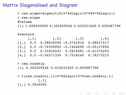
Matrix Diagonalised and Diagram> res.eigen=eigen(t(X)%*%diag(r)%*%X%*%diag(c))> res.eigen$values[1] 1.000000000 0.302459246 0.032631660 0.005687796

$vectors[,1] [,2] [,3] [,4]

[1,] 0.5 0.58634594 -0.2752916 0.08027417[2,] 0.5 -0.74350003 -0.1444609 -0.05137694[3,] 0.5 0.31830243 0.5814691 -0.61374293[4,] 0.5 -0.04571334 0.7518240 0.78373215

> res.coa$eig[1] 0.302459246 0.032631660 0.005687796

> t(res.coa$co[,1])%*%diag(c)%*%res.coa$co[,1][,1]

[1,] 0.3024592

..... ..... ..... . ..................... ..................... ..................... ..... ..... . ..... ..... ..... .

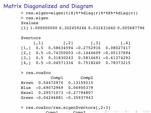
Matrix Diagonalized and Diagram> res.eigen=eigen(t(X)%*%diag(r)%*%X%*%diag(c))> res.eigen$values[1] 1.000000000 0.302459246 0.032631660 0.005687796

$vectors[,1] [,2] [,3] [,4]

[1,] 0.5 0.58634594 -0.2752916 0.08027417[2,] 0.5 -0.74350003 -0.1444609 -0.05137694[3,] 0.5 0.31830243 0.5814691 -0.61374293[4,] 0.5 -0.04571334 0.7518240 0.78373215

> res.coa$coComp1 Comp2

Brown 0.54472970 0.13159215Blue -0.69072969 0.06905379Hazel 0.29571073 -0.27794807Green -0.04246881 -0.35937943

> res.coa$co/res.eigen$vectors[,2:3]Comp1 Comp2

Brown 0.9290244 -0.4780101Blue 0.9290244 -0.4780101Hazel 0.9290244 -0.4780101Green 0.9290244 -0.4780101

..... ..... ..... . ..................... ..................... ..................... ..... ..... . ..... ..... ..... .

Part II

Inference: Confirmatory DataAnalysis

Stability (Internal and External)Hypothesis Testing

Evaluation

..... ..... ..... . ..................... ..................... ..................... ..... ..... . ..... ..... ..... .

▶ The statistical paradigm.

▶ Estimates and confidence.

▶ Statistical approaches to variability.

▶ Robustness

▶ Not always just multivariate vectors.

▶ Building a space for any object with a natural distance.

▶ The Bootstrap.

▶ Special cases: multivariate statistics and Treespace

Estimate τ̂ computed from the data: ..... ..... ..... . ..................... ..................... ..................... ..... ..... . ..... ..... ..... .

Data

..... ..... ..... . ..................... ..................... ..................... ..... ..... . ..... ..... ..... .

▶ BinaryLemur_cat 00000000000001010100000Tarsius_s 10000010000000010000000Saimiri_s 10000010000001010000000Macaca_sy 00000000000000010000000Macaca_fa 10000010000000010000000

▶ AlignedDNA Data for 12 species of primatesMitochondria, 898 characters on 12 species,( Hayasaka, K., T. Gojobori, and S. Horai. 1988).

12 60Lemur_cat AAGCTTCATA GGAGCAACCA TTCTAATAAT CGCACATGGC CTTACATCAT CCATATTATTTarsius_s AAGTTTCATT GGAGCCACCA CTCTTATAAT TGCCCATGGC CTCACCTCCT CCCTATTATTSaimiri_s AAGCTTCACC GGCGCAATGA TCCTAATAAT CGCTCACGGG TTTACTTCGT CTATGCTATTMacaca_sy AAGCTTCTCC GGTGCAACTA TCCTTATAGT TGCCCATGGA CTCACCTCTT CCATATACTTMacaca_fa AAGCTTCTCC GGCGCAACCA CCCTTATAAT CGCCCACGGG CTCACCTCTT CCATGTATTTMacaca_mu AAGCTTTTCT GGCGCAACCA TCCTCATGAT TGCTCACGGA CTCACCTCTT CCATATATTT

These data sets usually come with their own metrics.

..... ..... ..... . ..................... ..................... ..................... ..... ..... . ..... ..... ..... .

The parameter is a semi-labeled binary Tree

1 3 2 4

leaves

0 root

inner edgesinne

r edg

es

Inner Node

..... ..... ..... . ..................... ..................... ..................... ..... ..... . ..... ..... ..... .

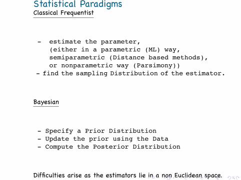
Statistical ParadigmsClassical Frequentist

- estimate the parameter,(either in a parametric (ML) way,semiparametric (Distance based methods),or nonparametric way (Parsimony))

- find the sampling Distribution of the estimator.

Bayesian

- Specify a Prior Distribution- Update the prior using the Data- Compute the Posterior Distribution

Difficulties arise as the estimators lie in a non Euclidean space...... ..... ..... . ..................... ..................... ..................... ..... ..... . ..... ..... ..... .

Sampling Distribution for Trees

Data 1

23

..... ..... ..... . ..................... ..................... ..................... ..... ..... . ..... ..... ..... .

..... ..... ..... . ..................... ..................... ..................... ..... ..... . ..... ..... ..... .

Data 1

23

Treespace Tn

..... ..... ..... . ..................... ..................... ..................... ..... ..... . ..... ..... ..... .

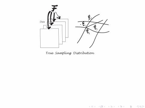
Data1

23

4

True Sampling Distribution

..... ..... ..... . ..................... ..................... ..................... ..... ..... . ..... ..... ..... .

Data1

23

4

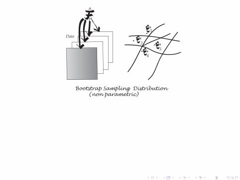
Bootstrap Sampling Distribution (non parametric)

n

^

*

**

*

..... ..... ..... . ..................... ..................... ..................... ..... ..... . ..... ..... ..... .

Data1

23

4

Bootstrap Sampling Distribution (parametric)

^

*

**

*

..... ..... ..... . ..................... ..................... ..................... ..... ..... . ..... ..... ..... .

How do we define distributions on Treespace

▶ Not the uniform distribution.▶ By inspiration from ranked Data: Mallow's model (1957)

P(τi) = Ke−λd(τi,τ0)

▶ Uses a central tree τ0.▶ Uses a distance d in treespace.▶ But very symmetrical, maybe need a mixture model.

▶ Other distributions (see Aldous, 2001), one might want toinclude information about the estimation method used asthis influences the shape of the tree.

..... ..... ..... . ..................... ..................... ..................... ..... ..... . ..... ..... ..... .

Classical Statistical Summaries

▶ Expectation (center of the distribution).Open question: What distribution is the consensus such acenter of?

▶ Median (multivariate median (Tukey, 1972).▶ Variance (second moment EPnd2(τ̂ , τ)).▶ Presence/Absence of a clade.▶ Summaries of Multivariate Variabilities. (PCA,MDS,..).

..... ..... ..... . ..................... ..................... ..................... ..... ..... . ..... ..... ..... .

Frequentist Confidence Regions

P(τ ∈ Rα) = 1− α

We will use the nonparametric approach of Tukey whoproposed peeling convex hulls to construct successive`deeper' confidence regions. But we need a geometricalspace to build these regions in. ..... ..... ..... . ..................... ..................... ..................... ..... ..... . ..... ..... ..... .

The Bootstrap

▶ What is the best estimate?(unbiased, most efficient)▶ How sure are we of the estimate? Confidence regions.

..... ..... ..... . ..................... ..................... ..................... ..... ..... . ..... ..... ..... .

Bootstrap support for Phylogenies Taking asobservations the columns of the matrix X ofaligned sequences, the rows representingthe species.The sampling distribution of the estimatedtree is estimated by resampling withreplacement among the characters orcolumns of the data.This provides a large set of plausiblealternative data sets, each be used in thesame way as the original data to give aseparate tree (see [5] for a review).

Parametric Bootstrapping for Microarray Clusters

..... ..... ..... . ..................... ..................... ..................... ..... ..... . ..... ..... ..... .

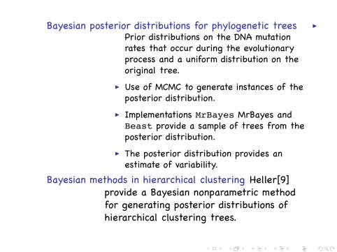
Bayesian posterior distributions for phylogenetic trees ▶

Prior distributions on the DNA mutationrates that occur during the evolutionaryprocess and a uniform distribution on theoriginal tree.

▶ Use of MCMC to generate instances of theposterior distribution.

▶ Implementations MrBayes MrBayes andBeast provide a sample of trees from theposterior distribution.

▶ The posterior distribution provides anestimate of variability.

Bayesian methods in hierarchical clustering Heller[9]provide a Bayesian nonparametric methodfor generating posterior distributions ofhierarchical clustering trees.

..... ..... ..... . ..................... ..................... ..................... ..... ..... . ..... ..... ..... .

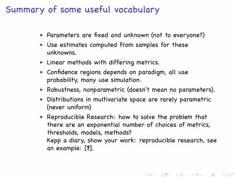
Summary of some useful vocabulary

▶ Parameters are fixed and unknown (not to everyone?)▶ Use estimates computed from samples for these

unknowns.▶ Linear methods with differing metrics.▶ Confidence regions depends on paradigm, all use

probability, many use simulation.▶ Robustness, nonparametric (doesn't mean no parameters).▶ Distributions in multivariate space are rarely parametric

(never uniform)▶ Reproducible Research: how to solve the problem that

there are an exponential number of choices of metrics,thresholds, models, methods?Kepp a diary, show your work: reproducible research, seean example: [?].

..... ..... ..... . ..................... ..................... ..................... ..... ..... . ..... ..... ..... .

Extensions

▶ Transformations that allow for nonlinearity (KernelPCA,etc).

▶ Transformation of variables to make them comparable(sphering).

▶ Transformation of variables to make them robust (ranks).

..... ..... ..... . ..................... ..................... ..................... ..... ..... . ..... ..... ..... .

Papers available here:http://www-stat.stanford.edu/˜susan/

..... ..... ..... . ..................... ..................... ..................... ..... ..... . ..... ..... ..... .

L. Billera, S. Holmes, and K. Vogtmann.The geometry of tree space.Adv. Appl. Maths, 771--801, 2001.

J. Chakerian and S. Holmes.Computational methods for evaluating phylogenetictrees, 2010.arXiv.P. Diaconis, S. Goel, and S. Holmes.Horseshoes in multidimensional scaling and kernelmethods.Annals of Applied Statistics, 2007.

B. Efron.Bootstrap methods: Another look at the jackknife.The Annals of Statistics, 7:1--26, 1979.

S. Holmes.Bootstrapping phylogenetic trees: theory andmethods.

..... ..... ..... . ..................... ..................... ..................... ..... ..... . ..... ..... ..... .

Statist. Sci., 18(2):241--255, 2003.Silver anniversary of the bootstrap.

Susan Holmes.Multivariate Analysis: The French way, volume 56 ofIMS Lecture Notes--Monograph Series.IMS, Beachwood, OH, 2006.

R. Ihaka and R. Gentleman.R: A language for data analysis and graphics.Journal of Computational and Graphical Statistics,5(3):299--314, 1996.

K. Mardia, J. Kent, and J. Bibby.Multiariate Analysis.Academic Press, NY., 1979.

R Savage, K Heller, Y Xu, and Z. Ghahramani.R/BHC: fast Bayesian hierarchical clustering formicroarray data.BMC, Jan 2009.

..... ..... ..... . ..................... ..................... ..................... ..... ..... . ..... ..... ..... .

I.J. Schoenberg.Remarks to Maurice Frechet's article ``Sur ladefinition axiomatique d'une classe d'espace distancesvectoriellement applicable sur l'esp ace de Hilbert.The Annals of Mathematics, 36(3):724--732, July1935.

..... ..... ..... . ..................... ..................... ..................... ..... ..... . ..... ..... ..... .