1

1

Multivariate Analysis forTOF-SIMS

©Copyright 1996-2007Eigenvector Research, Inc.No part of this material may bephotocopied or reproduced in any formwithout prior written consent fromEigenvector Research, Inc.

Barry M. Wise

2

Contact Information

Eigenvector Research, Inc.3905 West Eaglerock DriveWenatchee, WA 98801 USAweb: www.eigenvector.com

Barry M. Wise, Ph.D.Presidente-mail: bmw@eigenvector.comphone: 509-662-9213

2

3

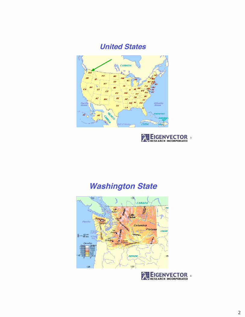
United States

4

Washington State

3

5

• Thinking Multivariate• General Principles• Data Sets• Pattern Recognition with Principal Components Analysis• Preprocessing• Supervised Pattern Recognition: Classification• Analysis of Multivariate Images• Self Modeling Mixture Analysis, aka Curve Resolution• Clustering• Conclusions

Outline

6

Definition of Chemometrics

Chemometrics is the chemical discipline thatuses mathematical and statistical methods to1) relate measurements made on a chemical

system to the state of the system2) design or select optimal measurement

procedures and experiments.

4

7

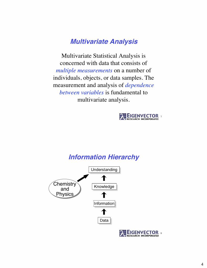
Multivariate Analysis

Multivariate Statistical Analysis isconcerned with data that consists of

multiple measurements on a number ofindividuals, objects, or data samples. Themeasurement and analysis of dependence

between variables is fundamental tomultivariate analysis.

8

Information Hierarchy

Understanding

Knowledge

Information

Data

Chemistry and

Physics

5

9

Motivation: Which Point isMost Unique?

0 10 20 30 40 50 60 70 80 90 100-4

-2

0

2

4

84

14

49

Sample

Var

iabl

e X

1

X1 with 95% Confidence Limits

0 10 20 30 40 50 60 70 80 90 100-4

-2

0

2

4

84

14

49

Sample

Var

iabl

e X

2

X2 with 95% Confidence Limits

10

Plot X2 versus X1

-3 -2 -1 0 1 2 3 4

-2.5

-2

-1.5

-1

-0.5

0

0.5

1

1.5

2

2.5

84

14

49

Variable X1

Var

iabl

e X

2

Variable X1 vs X2

6

11

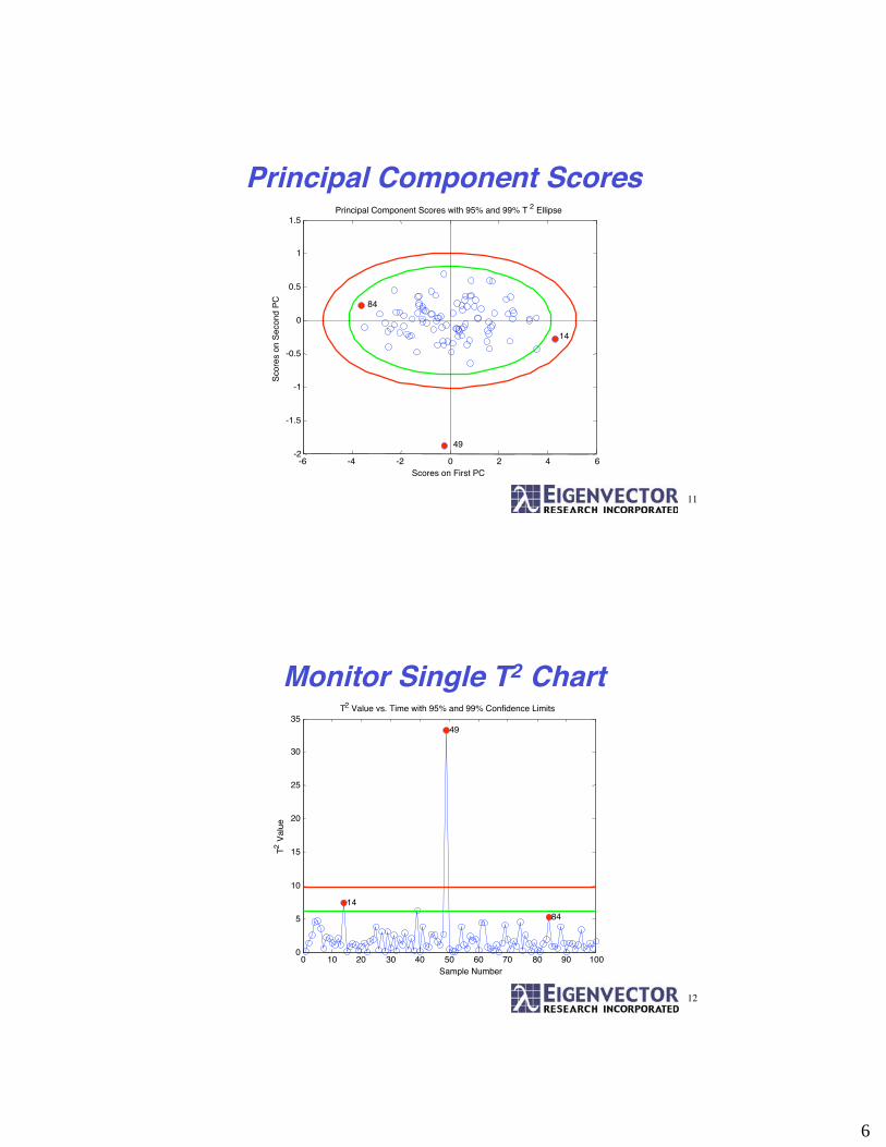
Principal Component Scores

-6 -4 -2 0 2 4 6-2

-1.5

-1

-0.5

0

0.5

1

1.5

84

14

49

Scores on First PC

Sco

res

on S

econ

d P

C

Principal Component Scores with 95% and 99% T 2 Ellipse

12

Monitor Single T2 Chart

0 10 20 30 40 50 60 70 80 90 1000

5

10

15

20

25

30

35

84

14

49

Sample Number

T2 V

alue

T2 Value vs. Time with 95% and 99% Confidence Limits

7

13

General Principles

• Balance• “Let the data speak for itself” - Bruce Kowalski• “Don’t estimate what you already know” - John

MacGregor

• Easier to fit data than predict it• Remember the parsimony principle• Validate models on independent test sets

• What you do before PCA, PLS etc. is critical• Experimental design, sample pedigree• Preprocessing to eliminate unwanted variance

14

Example Data Set 1

• Tyrosine-derived polyarylates

• From polymerization of diacids and diphenols

• Backbone length varied (X)

• Pendent (side) chain length varied (Y)

CH 2 CH2 C

O

NH CH CH 2

C O

O

CYH(2Y+1)

O C

O

C

O

O (CH2)X

DiacidDiphenol

Thanks to Anna Belu!

8

15

Example Data Set 2

• Multilayer drug bead-controlled release deliverysystem

• TOF-SIMS taken of crosssection of bead

• Evaluate integrity of layers,distribution of consituents

Thanks to Anna Belu!

A.M. Belu et. al., “TOF-SIMS Characterization and Imaging ofControlled-Release Drug Delivery Systems, Anal. Chem., 72(22),pps 5625-5638, 2000.

50 100 150 200 250

50

100

150

200

250

16

Principal ComponentsAnalysis

0

2

4

6

0

2

4

60

2

4

6

8

PC 1

Variable 1

Variable 2

Var

iable

3

Mean Vector

PC 2

9

17

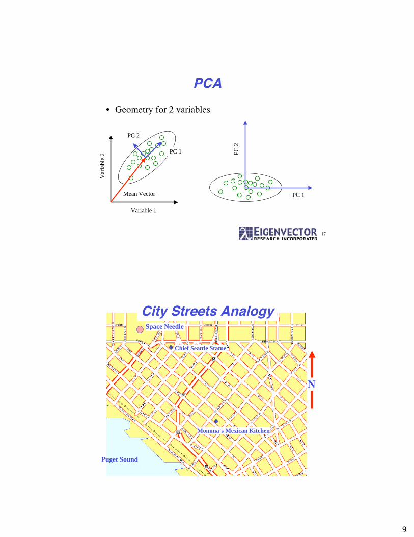
PCA

• Geometry for 2 variables

Variable 1

Var

iable

2

Mean Vector

PC 1

PC 2

PC 1

PC

2

City Streets Analogy

Puget Sound

Space Needle

Chief Seattle Statue

Momma’s Mexican Kitchen

N

10

19

Where q min{m,n}, and the tipiT pairs are ordered by the

amount of variance captured.

Generally, the model is truncated, leaving some small amount of variance in a residual matrix:

For a data matrix X with m samples and n variables (generallyassumed to be mean centered and properly scaled), the PCAdecomposition is:

X = t1p1T + t2p2

T + ... + tkpkT + ... + tqpq

T

X = t1p1T + t2p2

T + ... + tkpkT + E = TkPk

T + E

PCA Math 1 of 2

20

PCA Math 2 of 2

The pi are eigenvectors of the covariance matrix of X

1-m )cov(

TXX

X =

iii )cov( ppX =

and i are eigenvalues.

Amount of variance captured by tipiT proportional to i.

11

21

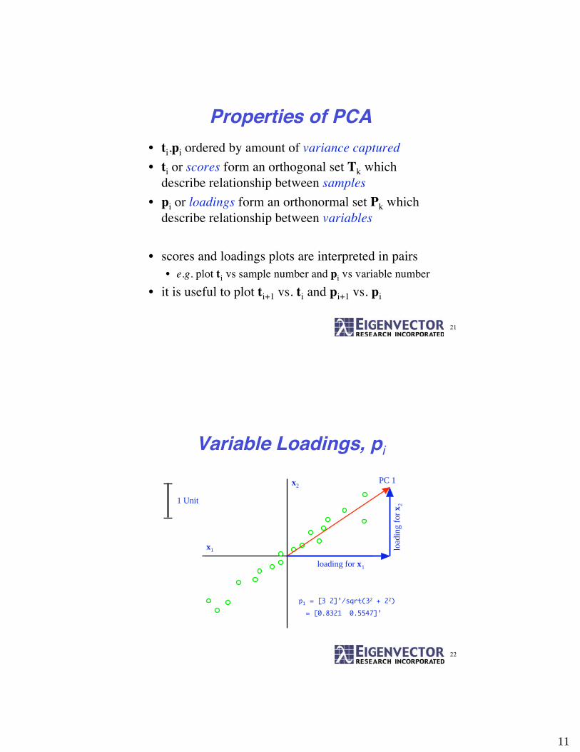
Properties of PCA• ti,pi ordered by amount of variance captured

• ti or scores form an orthogonal set Tk whichdescribe relationship between samples

• pi or loadings form an orthonormal set Pk whichdescribe relationship between variables

• scores and loadings plots are interpreted in pairs• e.g. plot ti vs sample number and pi vs variable number

• it is useful to plot ti+1 vs. ti and pi+1 vs. pi

22

PC 1

p1 = [3 2]’/sqrt(32 + 22)

= [0.8321 0.5547]’

1 Unit

Variable Loadings, pi

x1

x2

loading for x1

load

ing f

or

x2

12

23

Sample Scores, ti

x1

x2PC 1

sample

score

t1 = [2.25 1]* [0.8321 0.5547]’

= 2.4368

1 Unit

24

Arylate DataRaw Data Mean-centered Data

Autoscale?

Dominated by low mass peaks

Where are high mass peaks?

13

25

PCA of Mean-centered Arylate Percent Variance Captured by PCA Model Principal Eigenvalue % Variance % VarianceComponent of Captured Captured Number Cov(X) This PC Total--------- ---------- ---------- ---------- 1 8.58e-04 62.01 62.01 2 1.95e-04 14.11 76.13 3 1.65e-04 11.90 88.03 4 6.87e-05 4.97 92.99

B2

B4

B6 B8

S2

S4

S6

S8

26

Log-decay ScalingRaw Data

14

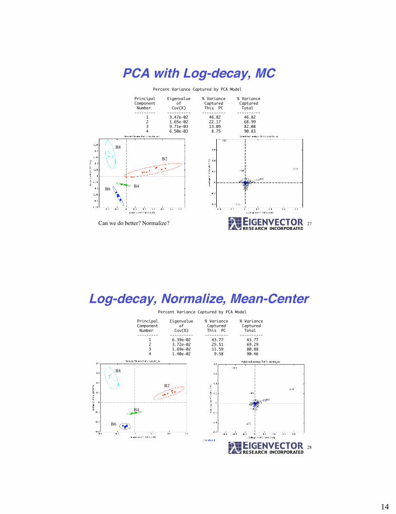
27

PCA with Log-decay, MC Percent Variance Captured by PCA Model Principal Eigenvalue % Variance % VarianceComponent of Captured Captured Number Cov(X) This PC Total--------- ---------- ---------- ---------- 1 3.47e-02 46.82 46.82 2 1.65e-02 22.17 68.99 3 9.71e-03 13.09 82.08 4 6.50e-03 8.75 90.83

B2

B4B6

B8

Can we do better? Normalize?

28

Log-decay, Normalize, Mean-Center Percent Variance Captured by PCA Model Principal Eigenvalue % Variance % VarianceComponent of Captured Captured Number Cov(X) This PC Total--------- ---------- ---------- ---------- 1 6.39e-02 43.77 43.77 2 3.72e-02 25.51 69.29 3 1.69e-02 11.59 80.88 4 1.40e-02 9.58 90.46

B2

B4

B6

B8

15

29

How Does it Work on theTest Set?

B2

B4

B6

B8

?

Check residuals!

?

30

Geometry of Q and T2

0

2

4

6

0

2

4

60

2

4

6

8 First PC

Second PC

Variable 1

Variable 2

Var

iable

3

Sample with large Q -Unusual variation outside the model

Sample with large T2

Unusual variation inside the model

16

31

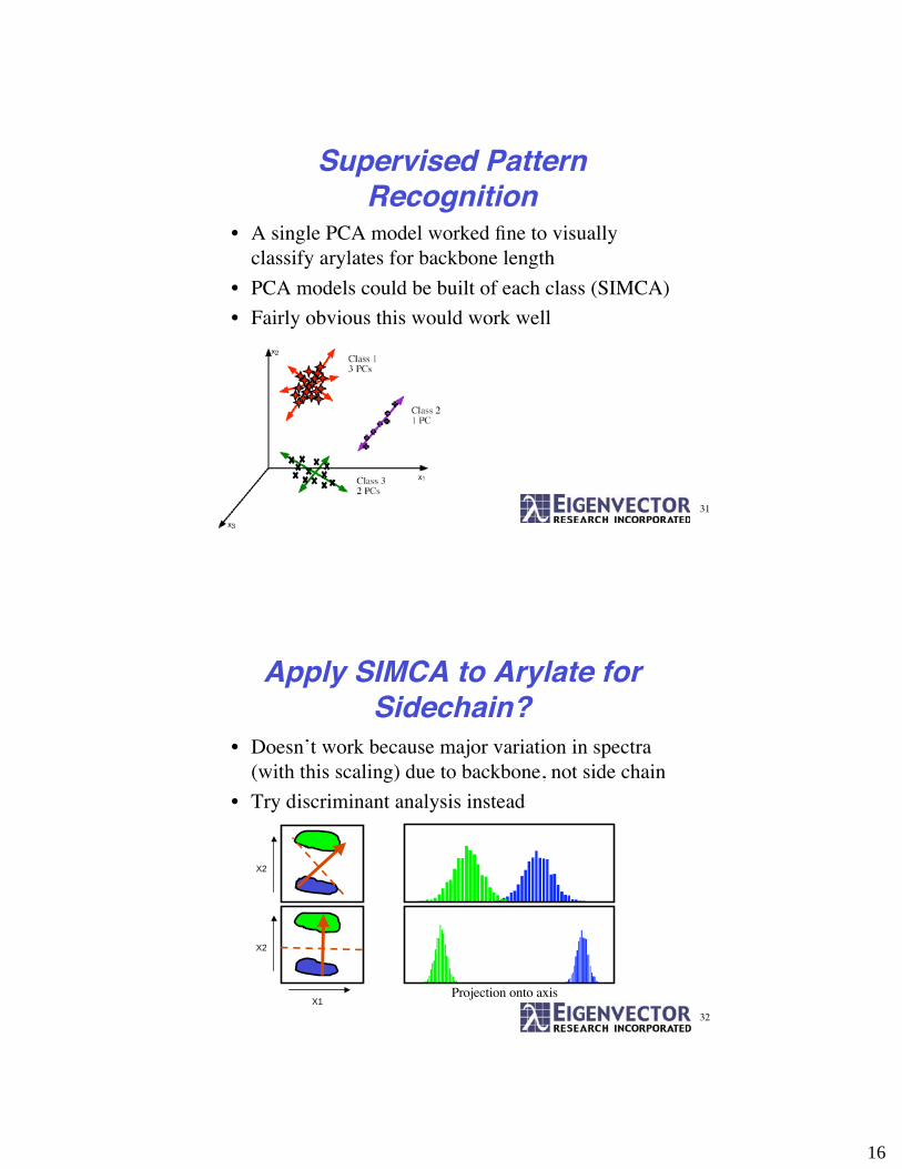
Supervised PatternRecognition

• A single PCA model worked fine to visuallyclassify arylates for backbone length

• PCA models could be built of each class (SIMCA)

• Fairly obvious this would work well

32

Apply SIMCA to Arylate forSidechain?

• Doesn’t work because major variation in spectra(with this scaling) due to backbone, not side chain

• Try discriminant analysis instead

Projection onto axisX1

X2

X2

17

33

Partial Least Squares DiscriminantAnalysis (PLS-DA)

• Use PLS regression to determine axis to projectdata on that discriminates between classes• choose axis so individual distributions are narrow

• choose axis so centers of distributions are far apart

• PLS is factor-based model of data therefore morestable with high collinearity.

• Will automatically attempt to identify directionsof interest!

34

PLS-DA for Sidechain Length

Calibration and testsamples shown

18

35

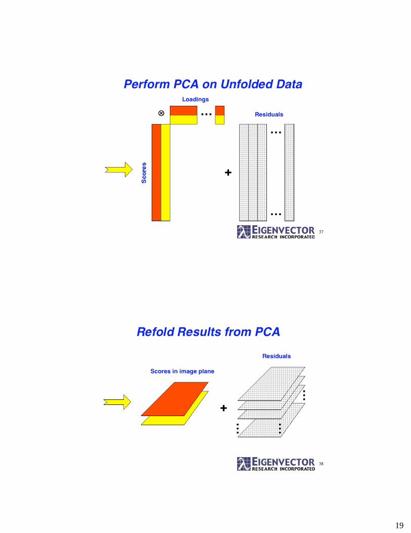
Image PCA

• SIMS images contain complete spectra for eachpixel

• Use PCA to condense information from allchannels down

• Use “scores” instead of single channels

36

19

37

38

20

39

40

21

41

42

22

43

44

23

45

46

24

47

48

25

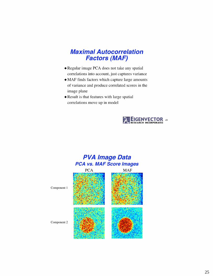
49

PVA Image DataPCA vs. MAF Score Images

PCA MAF

Component 1

Component 2

26

51

MCR Objective• Decompose a data matrix into chemically

meaningful factors• pure analyte spectra• pure analyte concentrations

• Easy to interpret• provides chemically / physically meaningful

information• caveats:

• rotational and multiplicative ambiguity• use of constraints

52

MCR

• Based on the classical least squares (CLS) model,attempt to estimate C and S given X:

X = CST+ E

where

X is a MxN matrix of measured responses,

C is a MxK matrix of pure analyte contributions,

S is a NxK matrix of pure analyte spectra, and

E is a MxN matrix of residuals.

Also called Self-modeling Mixture Analysis

27

53

Alternating Least Squares• How can we improve estimates of S and C?

• Given initial guess S0 (or C0)...

Ci = XSi-1(Si-1TSi-1)-1

Si = (CiTCi)-1Ci

T X• Iterate until convergence (ALS)

• Usually constrained such that C>0 and S>0

• and each skTsk=1

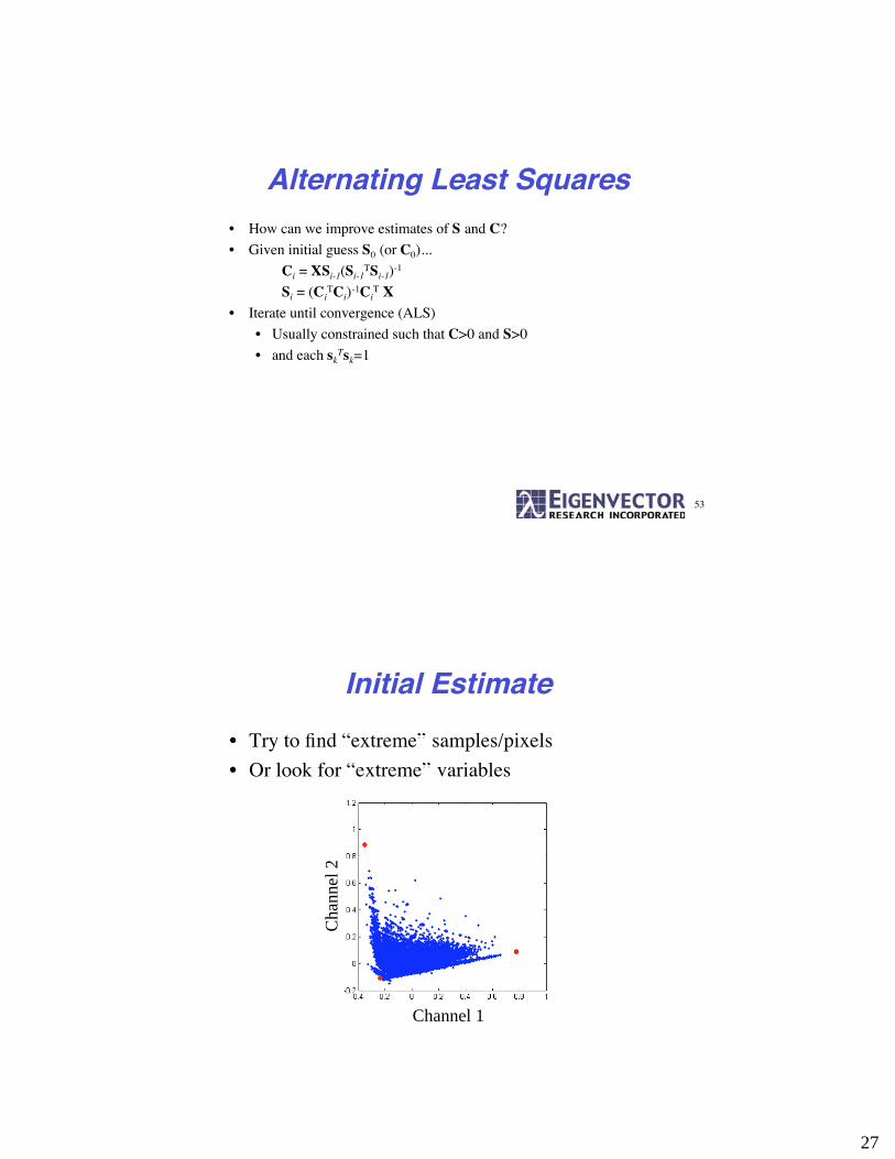
Initial Estimate

• Try to find “extreme” samples/pixels

• Or look for “extreme” variables

Ch

ann

el 2

Channel 1

28

55

MCR (ALS) on TOF-SIMS Image

• Non-negative constraints on both C and S

• Initialize with pure samples (i.e. pixels)

• Recover 6 interpretable spectra and concentrationprofiles

• Showing Score Images – image was unfolded witheach pixel as a separate sample then the scores arere-folded to form images

56

0 100 200 300 400 500 6000

0.2

0.4

0.6

0.8

1

589: Prednisolone +

Na+

365: Lactose + Na+

Prednisolone:

C21H31NaO9S

Lactose:

C12H22O11

50 100 150 200 250

50

100

150

200

2500

50

100

150

200

250

29

57

0 100 200 300 400 500 6000

0.2

0.4

0.6

0.8

1

23: Na+

50 100 150 200 250

50

100

150

200

2500

50

100

150

200

250

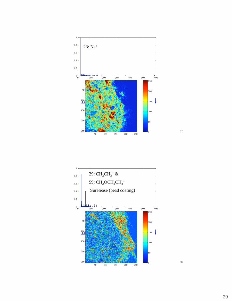
58

0 100 200 300 400 500 6000

0.2

0.4

0.6

0.8

1

29: CH2CH3+ &

59: CH2OCH2CH3+

Surelease (bead coating)

50 100 150 200 250

50

100

150

200

2500

50

100

150

200

250

30

59

RGB “Chemical” Image

50 100 150 200 250

50

100

150

200

250

Red: Surelease (bead coating)

Green: Na

Blue: Prednisolone (drug)

only 3 of 6 factors extracted

are shown

0 100 200 300 400 500 6000

0.2

0.4

0.6

0.8

1

41: “typical low mass

hydrocarbon” (CH2CH2CH3)

50 100 150 200 250

50

100

150

200

2500

50

100

150

200

250

31

0

0.1

0.2

0.3

0.4

0.5

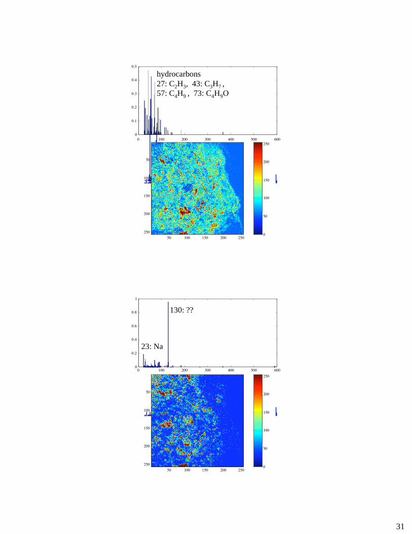
0 100 200 300 400 500 600

hydrocarbons

27: C2H3, 43: C3H7 ,

57: C4H9 , 73: C4H9O

50 100 150 200 250

50

100

150

200

2500

50

100

150

200

250

0 100 200 300 400 500 6000

0.2

0.4

0.6

0.8

1

130: ??

23: Na

50 100 150 200 250

50

100

150

200

2500

50

100

150

200

250

32

63

k-Means Agglomerative Clustering

12

3

4 5

6

7

• Samples are paired with anothersample or a cluster one-at-a-time

• Position of each cluster is meanof all samples in cluster.

• Recalculation of distance cantake a long time with lots ofsamples

64

KNN vs. K-MeansTwo clusters are grouped together when…

KNN…two of their members are theclosest of all dissimilar samples

x

x

x

K-Means …the cluster means are the closest

of all cluster means

x = cluster meanNote: these rules apply even when one of the“groups” is a single sample in a group of its own.

33

65

k-Means Partitional Clustering• Choose k samples as cluster “targets”

• random selection of samples• “pure samples”: choose samples on outside of data

(furthest from all other samples)

• Classify all samples into one of those k clusters.• Calculate mean of each cluster’s samples• Repeat classification and cluster means until no

samples are re-classed after mean recalculation.• Much faster, but dependent on initial guess of

samples

66

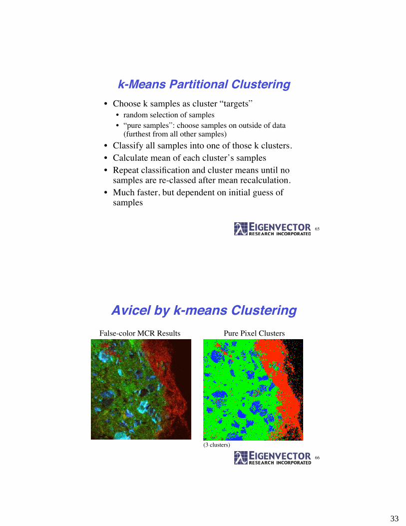
Avicel by k-means Clustering

False-color MCR Results Pure Pixel Clusters

(3 clusters)

34

67

Why Multivariate and FactorBased Methods?

• Noise filtering

• Selectivity enhancement

• Interpretation

• It’s a multivariate world!

68

Chemometrics SoftwareAdvanced Chemometric Software at Your Command

Eigenvector offers a

range of prepackaged

and custom software

products. Both as

add-ond to MATLAB

and as stand-alone

software.

35

69

Resources• Books• Chemometrics, M.A. Sharaf, D.L. Illman and B.R. Kowalski, Wiley-Interscience (1986) ISBN 0-471-83106-9• Multivariate Analysis, K.V. Mardia, J.I. Kent and J.M. Bibby, Academic Press, (1979) ISBN 0-12-471252-2• Multivariate Calibration, H. Martens and T. Næs, John Wiley & Sons Ltd. (1989) ISBN 0-471-90979-3• Chemometrics: a textbook, D.L. Massart et al., Elsevier (1988) ISBN 0-444-42660-4• Chemometrics: A Practical Guide, K.R. Beebe, R.J. Pell, M.B. Seasholtz, Wiley (1998) ISBN 0-471-12451-6• Multivariate Data Analysis In Practice, Kim H. Esbensen, CAMO ASA (2000), ISBN 82-993330-2-4• A user-friendly guide to Multivariate Calibration and Classification, T. Næs, T. Isaksson, T. Fearn, T. Davies, NIR

Publications(2002), ISBN 0-9528666-2-5• Multivariate Image Analysis, Paul Geladi and Hans Grahn, Wiley (1996), ISBN 0-471-93001-6• Multivariate Analysis of Quality: An Introduction, H. Martens and M. Martens, Wiley (2001), ISBN 0-471-97428-5

• Journals• Journal of Chemometrics• Chemometrics and Intelligent Laboratory Systems• Analytical Chemistry• Analytica Chemica Acta• Applied Spectroscopy• Critical Reviews in Analytical Chemistry• Journal of Process Control• Computers in Chemical Engineering• Technometrics• ....

70